Minimum-Cost Bounded-Degree Spanning Trees
36
Minimum-cost Bounded-degree Spanning Trees Feliciano Colella 17th December 2014
-
Upload
feliciano-colella -
Category
Science
-
view
28 -
download
1
Transcript of Minimum-Cost Bounded-Degree Spanning Trees

Minimum-cost Bounded-degree Spanning Trees
Feliciano Colella
17th December 2014

Introduction Approximation factor bv + 2 Approximation factor bv + 1 Further proofs and analysis
Outline
1 Definition of the problem;
2 Algorithm with approximation factor bv + 2;
3 Algorithm with approximation factor bv + 1;
4 Further analysis and some proofs.
Uncovered It is NP-complete to decide whether or not a givengraph has a minimum-degree spanning tree ofmaximum degree two.
Feliciano Colella Minimum-cost Bounded-degree Spanning Trees

Introduction Approximation factor bv + 2 Approximation factor bv + 1 Further proofs and analysis
The minimum-cost bounded-degree spanning tree problem
Input
• Undirected graph G = (V ,E ),
• Costs ce ≥ 0 for all e ∈ E ,
• A set W ⊆ V , with bounds bv ≥ 1 for all v ∈W .
Output
The minimum spanning tree (MST) such that the degree of eachnode v ∈W is no more than bv , it cannot exists.Let OPT be the cost of the MST.
Feliciano Colella Minimum-cost Bounded-degree Spanning Trees

Introduction Approximation factor bv + 2 Approximation factor bv + 1 Further proofs and analysis
Linear Programming formulation
Given a vertex set S ⊆ V , let:
• E (S) subset of edges in E that have both endpoints in S ,
• δ(S) subset of edges that have only one endpoint in S ,
xe ∈ {0, 1} indicate whether e is in the ST or not.
Feliciano Colella Minimum-cost Bounded-degree Spanning Trees

Introduction Approximation factor bv + 2 Approximation factor bv + 1 Further proofs and analysis
Linear Programming formulation
minimize∑e∈E
cexe
subject to∑e∈E
xe = |V | − 1,∑e∈E(S)
xe ≤ |V | − 1, ∀S ⊆ V , |S | ≥ 2,∑e∈δ(v)
xe ≤ bv , ∀v ∈W ,
xe ≥ 0, ∀e ∈ E .
Can be solved with ellipsoid method by giving a polynomial-timeseparation oracle.
Feliciano Colella Minimum-cost Bounded-degree Spanning Trees

Introduction Approximation factor bv + 2 Approximation factor bv + 1 Further proofs and analysis
A sequence of Max-Flow problems
Create a new graph G ′ where we add two vertices s and t, and weadd edges (s, v) and (v , t) for each v ∈ V .The capacity of e ∈ G is 1
2xe , 12
∑e∈δ(v) xe for every edge (s, v)
and 1 for every edge (v , t), the total is:
|S |+ 1
2
∑e∈δ(S)
xe +1
2
∑v /∈S
∑e∈δ(v)
xe = |S |+∑
e∈δ(S)
xe +∑
e∈E(V−S)
xe
Using that∑
e∈E xe = |V | − 1 we have:
|S |+ |V | − 1−∑
e∈E(S)
xe = |V |+ (|S |+ 1)−∑
e∈E(S)
xe
The capacity of this cut is at least |V | ⇐⇒∑
e∈E(S)
xe ≥ |S | − 1
We want |S | ≥ 2 for each pair x , y ∈ V , how ?
Feliciano Colella Minimum-cost Bounded-degree Spanning Trees

Introduction Approximation factor bv + 2 Approximation factor bv + 1 Further proofs and analysis
An algorithm for the case W = ∅
Theorem
Algorithm below yields a spanning tree of no more than the valueof the linear program.
F ← ∅while |V | > 1 do
Solve LP on (V ,E ), basic solution is xE ← E (x)Find v ∈ V s.t. there is only one edge (u, v) incident on vF ← F ∪ {(u, v)}V ← V − {v}E ← E − {(u, v)}
return F
Feliciano Colella Minimum-cost Bounded-degree Spanning Trees

Introduction Approximation factor bv + 2 Approximation factor bv + 1 Further proofs and analysis
Returning to our problem ...
... we show two main results:
Lemma
For any basic feasible solution x to the linear program, either thereis some v ∈ V such that there is at most one edge of E (x)incident on v , or there is some v ∈W such that there are at mostthree edges of E (x) incident on v .
Theorem
The next algorithm produces a spanning tree F such that thedegree of v ∈ F is at most bv + 2 for v ∈W , and such that thecost of F is at most the value of the linear program.
Feliciano Colella Minimum-cost Bounded-degree Spanning Trees
Introduction Approximation factor bv + 2 Approximation factor bv + 1 Further proofs and analysis
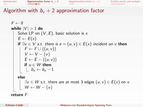
Algorithm with bv + 2 approximation factor
F ← ∅while |V | > 1 do
Solve LP on (V ,E ), basic solution is xE ← E (x)if ∃v ∈ V s.t. there is e = (u, v) ∈ E (x) incident on v then
F ← F ∪ {(u, v)}V ← V − {v}E ← E − {(u, v)}if u ∈W then
bu ← bu − 1
else∃v ∈W s.t. there are at most 3 edges (u, v) ∈ E (x) on vW ←W − {v}
return F
Feliciano Colella Minimum-cost Bounded-degree Spanning Trees

Introduction Approximation factor bv + 2 Approximation factor bv + 1 Further proofs and analysis
Proof of the previous Theorem
• Each step add edge to F or remove vertex from W , thus(n − 1) + 1 = 2n − 1 iterations.
• Proof of the cost of the spanning tree still holds from theprevious theorem, we need to consider the set of bounds W .
• Since x was feasible for the constraint∑
e∈δ(u) xe ≤ bu, thenif we remove e = (v , u) with xe = 1 from the graph, we havethat x is still feasible on new graph with bound bu − 1.
Now consider a vertex v initially in W , its degree in F will be atmost bv + 2.
Feliciano Colella Minimum-cost Bounded-degree Spanning Trees

Introduction Approximation factor bv + 2 Approximation factor bv + 1 Further proofs and analysis
Proof of the previous Theorem
By cases:
1 The edge is incident on v , bv decrease by 1;
2 The edge is incident on v and v is removed from the graph:• we must have had bv ≥ 1 to have a feasible solution, so the
statement holds.
3 The node v is removed from W :• we must have had bv ≥ 1 for there to be any edges in E (x)
incident on v ;• there are at most 3 edges in E (x) incident on v ;• we can add at most all of the 3 edges, so the degree will be at
most bv + 2
�
Feliciano Colella Minimum-cost Bounded-degree Spanning Trees

Introduction Approximation factor bv + 2 Approximation factor bv + 1 Further proofs and analysis
A better algorithm
We give now an algorithm that finds a spanning tree of cost atmost OPT such that each node v ∈W has degree at most bv + 1.
while W 6= ∅ doSolve LP on (V ,E ),W , get basic optimal solution is xE ← E (x)Select v ∈W such that there are at most bv + 1 edges in Eincident on vW ←W − {v}
Compute minimum-cost ST F on (V ,E )return F
Feliciano Colella Minimum-cost Bounded-degree Spanning Trees

Introduction Approximation factor bv + 2 Approximation factor bv + 1 Further proofs and analysis
The key of the proof
The key idea is to state and prove a stronger lemma than theprevious one:
Lemma
For any basic feasible solution x to the LP in which W 6= ∅, thereis some v ∈W such that there are at most bv + 1 edges incidenton v in E (x).
Which leads to the theorem:
Theorem
The previous algorithm produces a spanning tree F such that thedegree of v ∈ F is at most bv + 1 for v ∈W , and such that thecost of F is at most the value of the linear program.
Feliciano Colella Minimum-cost Bounded-degree Spanning Trees

Introduction Approximation factor bv + 2 Approximation factor bv + 1 Further proofs and analysis
Proof of the algorithm with approx factor bv + 1
Proof.
• By induction on iterations, if xe is feasible for (V ,E ),W itwill still be on (V ,E ′),W ′;
• We remove e from E if xe = 0, or we remove v from W ,imposing fewer constraint.
• Those removals does not affect the feasibility of the solution;
• Since we can remove a vertex from W , eventually W = ∅;• When we modify E and W , the value of LP never increase;
• The cost of the MST is at most the value of the LP;
• We removed v from W only if there were at most bv + 1edges remaining (in E on v);
• The spanning tree can have at most degree bv + 1,∀v ∈W .
Feliciano Colella Minimum-cost Bounded-degree Spanning Trees

Introduction Approximation factor bv + 2 Approximation factor bv + 1 Further proofs and analysis
Starting definitions
From now on, assume that the edges e s.t. xe = 0, has beenremoved, so E = E (x).
Definition 11.7 given a subset F , we define x(F ) =∑
e∈F xe ;
Definition 11.8 given x , a constraint is tight if x(E (S)) = |S | − 1or x(δ(v)) = bv ;
Definition 11.9 A and B are intersecting if A ∩ B, A− B andB − A are all non empty;
Definition 11.10 S is laminar if no pair of sets A,B ∈ S areintersecting;
Definition 11.11 given a subset F ⊆ E , the characteristic vector isχF ∈ {0, 1}|E |, where χF (e) = 1 if e ∈ F .
Feliciano Colella Minimum-cost Bounded-degree Spanning Trees

Introduction Approximation factor bv + 2 Approximation factor bv + 1 Further proofs and analysis
Some useful Results
Lemma 11.13
Let L be a laminar collection of subset of V , where each S ∈ Lhas |S | ≥ 2. Then |L| ≤ |V | − 1.
Proof.
Induction on |V |. Base |V | = 2, L only contains one set of size 2.For |V | ≥ 2:
• pick R ∈ L with minimum cardinality
• let V ′ be V \R and L′ the sets restricted to V ′
• L′ is still laminar, so |L′| ≤ |V ′| − 1 by induction
• since |L′| = |L| − 1 and |V ′| = |V | − 1 the statement follows
Feliciano Colella Minimum-cost Bounded-degree Spanning Trees

Introduction Approximation factor bv + 2 Approximation factor bv + 1 Further proofs and analysis
Some useful Results
Lemma 11.14
If S and T are tight sets such that S and T are intersecting, thenS ∪ T and S ∩ T are also tight sets. Furthermore,
χE(S) + χE(T ) = χE(S∪T ) + χE(S∩T )
Let T = {S ⊆ V : x(E (S)) = |S | − 1, |S | ≥ 2} be the collection ofall the tight sets for the LP solution x .Let span(T ) = {χE(S) : S ∈ T } be the span of that sets of vectors.
Lemma 11.15
There exists a laminar collection of sets L such thatspan(L) ⊇ span(T ), where each S ∈ L is tight and has |S | ≥ 2,and the vectors χE(S) for S ∈ L are linearly independent.
Feliciano Colella Minimum-cost Bounded-degree Spanning Trees

Introduction Approximation factor bv + 2 Approximation factor bv + 1 Further proofs and analysis
Some useful Results
Theorem 11.12
For any basic feasible solution x to the LP, there is a set Z ⊆Wand a collection L of subsets of vertices with the followingproperties:
1 For all S ∈ L, |S | ≥ 2 and S is tight, and for all v ∈ Z , v istight.
2 The vectors χE(S) for S ∈ L and χδv) ∈ Z are linearlyindependent.
3 |L| = |Z |+ |E |.4 The collection L is laminar.
Feliciano Colella Minimum-cost Bounded-degree Spanning Trees

Introduction Approximation factor bv + 2 Approximation factor bv + 1 Further proofs and analysis
Some useful Results
Lemma 11.18
For any e ∈ E such that xe = 1, χe ∈ span(L).Proof Follows from the previous theorem.
Lemma 11.16
For any basic feasible solution x to the LP in which W 6= ∅, thereis some v ∈W such that there are at most bv + 1 edges incidenton v in E (x).
Feliciano Colella Minimum-cost Bounded-degree Spanning Trees

Introduction Approximation factor bv + 2 Approximation factor bv + 1 Further proofs and analysis
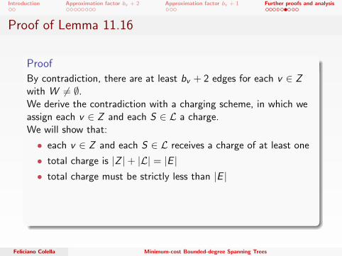
Proof of Lemma 11.16
Proof
By contradiction, there are at least bv + 2 edges for each v ∈ Zwith W 6= ∅.We derive the contradiction with a charging scheme, in which weassign each v ∈ Z and each S ∈ L a charge.
We will show that:
• each v ∈ Z and each S ∈ L receives a charge of at least one
• total charge is |Z |+ |L| = |E |• total charge must be strictly less than |E |
Assign a charge of 12(1− xe) to each endpoint of e ∈ Z , and assign
of xe to the smallest S ∈ L that contains both endpoints of e, ifexists. Notice that the total charge is at most 1 per edge e ∈ E .
Feliciano Colella Minimum-cost Bounded-degree Spanning Trees
Introduction Approximation factor bv + 2 Approximation factor bv + 1 Further proofs and analysis
Proof of Lemma 11.16
Proof
By contradiction, there are at least bv + 2 edges for each v ∈ Zwith W 6= ∅.We derive the contradiction with a charging scheme, in which weassign each v ∈ Z and each S ∈ L a charge.We will show that:
• each v ∈ Z and each S ∈ L receives a charge of at least one
• total charge is |Z |+ |L| = |E |• total charge must be strictly less than |E |
Assign a charge of 12(1− xe) to each endpoint of e ∈ Z , and assign
of xe to the smallest S ∈ L that contains both endpoints of e, ifexists. Notice that the total charge is at most 1 per edge e ∈ E .
Feliciano Colella Minimum-cost Bounded-degree Spanning Trees

Introduction Approximation factor bv + 2 Approximation factor bv + 1 Further proofs and analysis
Proof of Lemma 11.16
Proof
Each v ∈ Z receives a charge of 12(1− xe) from each edge of E
incident. By hypothesis, there are at least bv + 2 edges on v .Since v ∈ Z implies v is tight, we know that
∑e∈δ(v) xe = bv , thus
the total is:
∑e∈δ(v)
1
2(1− xe) =
1
2
|δ(v)| −∑
e∈δ(v)
xe
≥ 1
2[(bv + 2)− bv ]
= 1.
Feliciano Colella Minimum-cost Bounded-degree Spanning Trees

Introduction Approximation factor bv + 2 Approximation factor bv + 1 Further proofs and analysis
Proof of Lemma 11.16
Proof
Consider a set S ∈ L. If S contains no other set C ∈ L, since S istight and |S | ≥ 2 then the total charge is at least 1. Suppose thatS has a child C ∈ L which is strictly contained in S . Let C1 . . .Ck
be the children of S , they are all tight and x(E (Ci )) = |Ci | − 1. Bylaminarity of L and for Theorem 11.12, the total charge to S is:
x(E (S))−k∑
i=1
x(E (Ci )) > 0
The following is integral, which leads to a charge of at least one
x(E (S))−k∑
i=1
x(E (Ci )) = (|S | − 1)−k∑
i=1
(|Ci | − 1)
Feliciano Colella Minimum-cost Bounded-degree Spanning Trees

Introduction Approximation factor bv + 2 Approximation factor bv + 1 Further proofs and analysis
Proof of Lemma 11.16
Proof.
We show that the total charge is less than |E | by cases:
1 If V /∈ L2 Exists some e = (u, v) ∈ E with xe < 1 s.t. one of its
endpoint is not in Z
3 Suppose V ∈ L and for any e ∈ E with xe < 1, bothendpoints of e are in Z .
1 Exists e /∈ E (S) ∀S ∈ L, charge xe > 0 is not made to anyset, so the total is strictly less than |E |.
2 Let u ∈ Z , his charge is not made to 12(1− xe) > 0.
3 This case lead to a contradiction (for 11.12), one of theprevious cases must occur (proved using lemma 11.18).
Feliciano Colella Minimum-cost Bounded-degree Spanning Trees

Questions?