Minimising Changeover Costs in the Heijunka Board with ... product mix in a Heijunka... · examples...

Harris, I. and Disney, S.M., (2014), “Levelling product mix in a Heijunka Board with shortest path algorithms”, Pre-prints of the 18th International Working Seminar of Production Economics, Innsbruck, Austria, February 24th–28th, Vol. 4, pp75–87.

1

Minimising Changeover Costs in the Heijunka Board with Shortest Path Algorithms

Irina Harris and Stephen M. Disney

Logistics Systems Dynamics Group, Cardiff Business School, Cardiff University, Aberconway Building, Colum Drive, Cardiff, CF10 3EU, UNITED KINGDOM.

[email protected], [email protected]

Abstract A Heijunka Board is a Lean Production technique that helps to communicate a timed production plan to the factory floor. Lean advocates that production plans should be generated to level the volume and to level the mix. It is the mix levelling aspect of the Heijunka Board that we are concerned with. In particular, given that a number of products have to be produced on a production line, the order or sequence of production is of importance. This is because changing from one product to the next in the sequence incurs a set-up or changeover cost. If the set-ups are different for each pair of products in a changeover, the question arises “which is the optimal sequence that minimises the total set-up costs as we go round the Product Wheel?” It is this question that we answer here. We show that this mixed model production schedule problem can be represented as a Directed Acyclic Graph (DAG) where the edges of the graph represent the changeover costs. This allows us to apply various Shortest Path Algorithms to minimise the total changeover associated with going through one complete cycle of the product range. We show how the Product Wheel can be formulated as a DAG and solved by hand for small cases when all the changeover over costs are non-negative. Here we use the intuitive, logarithmic time, Dijkstra’a Shortest Path Algorithm (DSPA). For larger problems we have developed both a User Defined Function in Excel and a Java application based on both Topological Sort Algorithm operating in linear time and DSPA. Numerical examples are provided to test the solution methods and computational results illustrate the effectiveness of both approaches to randomly generated problem instances. Key words: Heijunka Board, Shortest Path, Directed Acyclic Graph, Changeover Costs, Product Wheel 1. Introduction One of central themes of the Lean Production philosophy is to only produce (or assemble) what you sell in each period – to match production to demand. In order to do this the demand volume in each day must be fairly level, otherwise there will be significant losses due to the (expensive) production capacity not matching the demand volume. It is well known that if customer orders are simply passed along to the production facility, the variability of those orders is likely to be less that if it passes through a “standard” inventory replenishment rule (such as the Order-Up-To policy with exponential smoothing forecasts), Dejonckheere et al (2003). With clever design these volume variability amplifying replenishment algorithms can be made to smooth the replenishment orders. However this is fairly difficult task, Disney et al (2013), and much of the Lean advice simply avoids this issue by recommending that production targets are set to the most recent demands in a “pass-on-orders” strategy. Another way to reduce volume variability is to make the replenishment periods as short as possible. This conceptually simple, easy to communicate strategy helps companies to reduce finished goods inventory levels, Hedenstierna and Disney (2012). Another aspect of the Lean Production philosophy recognises that products rarely have a dedicated production line. In most cases several products share the same production facilities. This implies that, intermittently, the production line needs to be changed in some manner to allow for a different product to be produced. This “set-up” or “changeover” takes time and costs money. The Lean approach advocates reducing the set-up cost (or set-up time) as much


2

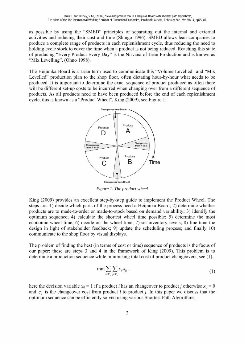
as possible by using the “SMED” principles of separating out the internal and external activities and reducing their cost and time (Shingo 1996). SMED allows lean companies to produce a complete range of products in each replenishment cycle, thus reducing the need to holding cycle stock to cover the time when a product is not being reduced. Reaching this state of producing “Every Product Every Day” is the Nirvana of Lean Production and is known as “Mix Levelling”, (Ohno 1998). The Heijunka Board is a Lean term used to communicate this “Volume Levelled” and “Mix Levelled” production plan to the shop floor, often dictating hour-by-hour what needs to be produced. It is important to determine the exact sequence of product produced as often there will be different set-up costs to be incurred when changing over from a different sequence of products. As all products need to have been produced before the end of each replenishment cycle, this is known as a “Product Wheel”, King (2009), see Figure 1.

Figure 1. The product wheel

King (2009) provides an excellent step-by-step guide to implement the Product Wheel. The steps are: 1) decide which parts of the process need a Heijunka Board; 2) determine whether products are to made-to-order or made-to-stock based on demand variability; 3) identify the optimum sequence; 4) calculate the shortest wheel time possible; 5) determine the most economic wheel time; 6) decide on the wheel time; 7) set inventory levels; 8) fine tune the design in light of stakeholder feedback; 9) update the scheduling process; and finally 10) communicate to the shop floor by visual displays.

The problem of finding the best (in terms of cost or time) sequence of products is the focus of our paper; these are steps 3 and 4 in the framework of King (2009). This problem is to determine a production sequence while minimising total cost of product changeovers, see (1),

minp p

ij iji V j V

c x , (1)

here the decision variable xij = 1 if a product i has an changeover to product j otherwise xij = 0 and ijc is the changeover cost from product i to product j. In this paper we discuss that the optimum sequence can be efficiently solved using various Shortest Path Algorithms.


3

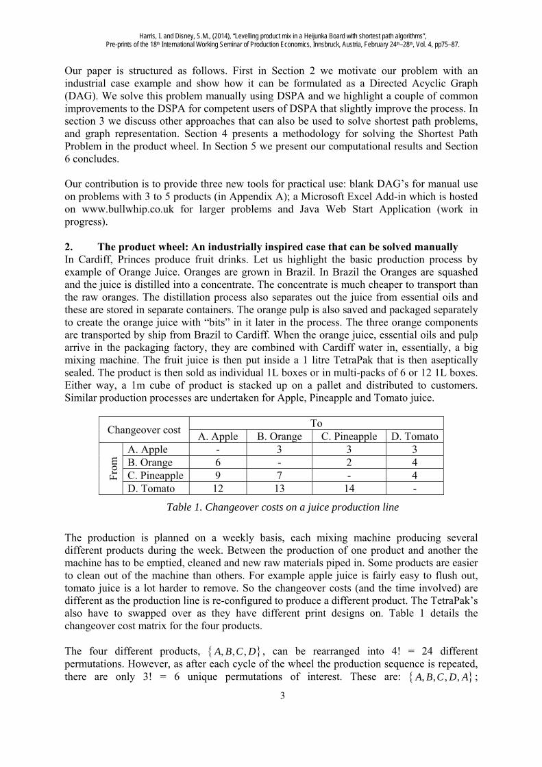
Our paper is structured as follows. First in Section 2 we motivate our problem with an industrial case example and show how it can be formulated as a Directed Acyclic Graph (DAG). We solve this problem manually using DSPA and we highlight a couple of common improvements to the DSPA for competent users of DSPA that slightly improve the process. In section 3 we discuss other approaches that can also be used to solve shortest path problems, and graph representation. Section 4 presents a methodology for solving the Shortest Path Problem in the product wheel. In Section 5 we present our computational results and Section 6 concludes. Our contribution is to provide three new tools for practical use: blank DAG’s for manual use on problems with 3 to 5 products (in Appendix A); a Microsoft Excel Add-in which is hosted on www.bullwhip.co.uk for larger problems and Java Web Start Application (work in progress). 2. The product wheel: An industrially inspired case that can be solved manually In Cardiff, Princes produce fruit drinks. Let us highlight the basic production process by example of Orange Juice. Oranges are grown in Brazil. In Brazil the Oranges are squashed and the juice is distilled into a concentrate. The concentrate is much cheaper to transport than the raw oranges. The distillation process also separates out the juice from essential oils and these are stored in separate containers. The orange pulp is also saved and packaged separately to create the orange juice with “bits” in it later in the process. The three orange components are transported by ship from Brazil to Cardiff. When the orange juice, essential oils and pulp arrive in the packaging factory, they are combined with Cardiff water in, essentially, a big mixing machine. The fruit juice is then put inside a 1 litre TetraPak that is then aseptically sealed. The product is then sold as individual 1L boxes or in multi-packs of 6 or 12 1L boxes. Either way, a 1m cube of product is stacked up on a pallet and distributed to customers. Similar production processes are undertaken for Apple, Pineapple and Tomato juice.

Changeover cost To

A. Apple B. Orange C. Pineapple D. Tomato

Fro

m A. Apple - 3 3 3

B. Orange 6 - 2 4 C. Pineapple 9 7 - 4 D. Tomato 12 13 14 -

Table 1. Changeover costs on a juice production line

The production is planned on a weekly basis, each mixing machine producing several different products during the week. Between the production of one product and another the machine has to be emptied, cleaned and new raw materials piped in. Some products are easier to clean out of the machine than others. For example apple juice is fairly easy to flush out, tomato juice is a lot harder to remove. So the changeover costs (and the time involved) are different as the production line is re-configured to produce a different product. The TetraPak’s also have to swapped over as they have different print designs on. Table 1 details the changeover cost matrix for the four products. The four different products, , , ,A B C D , can be rearranged into 4! = 24 different permutations. However, as after each cycle of the wheel the production sequence is repeated, there are only 3! = 6 unique permutations of interest. These are: , , , ,A B C D A ;


4

, , , ,A B D C A ; , , , ,A C B D A ; , , , ,A C D B A ; , , , ,A D B C A ; and , , , ,A D C B A . Notice, here we have returned the wheel to its starting position that we arbitrarily choose to be product A. These six unique permutations can be represented as a DAG, with the edges representing the changeover cost (or time or other utility) and the vertexes representing the products (and, importantly its predecessors), see Figure 2 (a). We have chosen DSPA for solving the DAG in this introductory example as it is intuitive and easy to visualise, although there are faster shortest path algorithms available and others that can cope with DAG’s with negative edge weights. The shortest path is identified in the following manner with DSPA where shortest path is visualised in Figure 2 (b):

Step 1. Shade all vertices reachable from the current set of reachable nodes. Step 2. Calculate the cost to reach all reachable nodes. Step 3. Pick the vertex with the smallest cost and deem it reached (if more than one node

has an equal smallest cost, pick one at random). Step 4. Repeat steps 1-3 until you reach the destination. Step 5. Determine the shortest path by working backward though the graph looking for

the route with the shortest distance. Figure 2 (b) shows the output of the DSPA for the juice problem. The shortest path has a total changeover cost of 21 and is the shortest path through the product wheel is , , , ,A B C D A .

Figure 2. The product wheel represented as a shortest path problem (a) solved using DPSA (b)

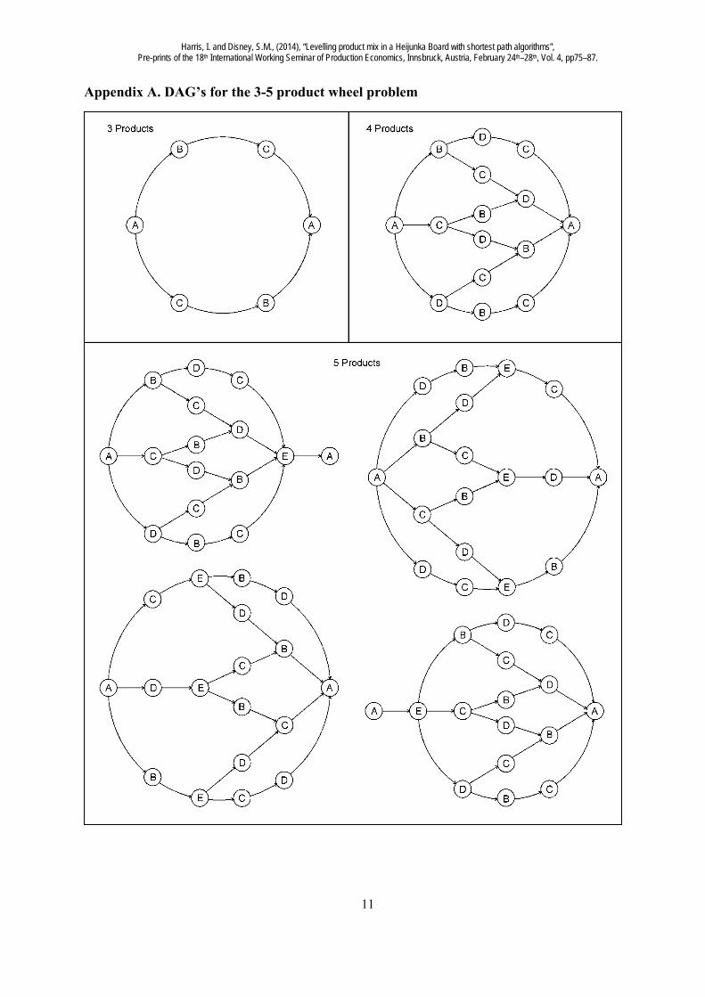
There are two common improvements to the DSPA. One is to take alternate step forwards and backwards through the DAG. The two paths will meet somewhere in the middle of the graph, highlighting the shortest path and distance by visiting less nodes within the DAG. Another variation is to first pre-process the DAG, consolidating nodes on a linear routes with no adjoin or diverging paths. However, it is unclear beforehand whether the pre-processing results in fewer calculations overall. The number of possible paths in the an n product wheel is 1 !n With 2 products there is only one route (sequence) though the wheel, 3 products imply 2 routes, 4 products produce 6 routes, 5 products require 24 routes and so on. It is possible to solve this scale of the problem by hand and we have provided in Appendix A the DAG’s required to undertake such as task


5

for easy reference. Notice, that the five products problem can be solved as four DAG’s simultaneously. However, for product wheels of six or more products the manual approach becomes unwieldy. Thus in the next section we turn our attention to computer based algorithms and solutions. 3. Computer based approaches to solving shortest path problems A number of algorithms exist to find shortest paths in DAGs. The DSPA and the Bellman-Ford algorithm and are two well-known approaches that compute shortest paths (Bertsekas and Gallager 1992, Salama et al. 1997). The Bellman-Ford algorithm is more flexible as it can handle graphs with negative weights but is slower than the DSPA.

Dijkstra’s shortest path algorithm was published in late 1959 by Edsger Dijkstra and used for solving shortest path problems with positive weights. It has been widely applied to routing problems in road and network protocols. The main idea of the algorithm is to search through each node of the graph that is located on the “unseen” shortest path from source to the destination node with the aim of finding the lowest cost solution. The algorithm stops when the shortest path to the destination node has been found. The algorithm operates in the logarithmic time.

The Topological Sort Algorithm (TSA) is another approach for solving the shortest path problems in DAG’s. The TSA orders vertices in a DAG in a way that if there is a path from vertices v1 to v2 then v1 appears before v2 in the topological order. If there are cycles in the graph, then a graph cannot have a topological order (Weiss 2006). We find however, that there are no cycles in our Product Wheel problem; hence we have an acyclic graph.

The manner in which we represent the DAG in a computer program has implications for memory use and speed. Getting it wrong will result in a program that will run out of memory. We explored two common data representations of the DAG’s: the adjacency matrix; and the adjacency list as illustrated in Table 2. The adjacency matrix is a two-dimensional array where cij is the edge cost and all non-zero values represent the cost of adjacency between two vertices. The matrix representation could be used for dense graphs (where the number of edges is close to the square of the number of vertices, |E| is close to |V|2) where information related to adjacency is stored in the matrix. However the adjacency matrix requires initialisation and this task has a cost that is quadratic in the number of nodes in the graph. In our relatively sparse matrix, the number of possible edges |E| is much less than the square of the vertices |V|2. Thus there is a need for a different data structure, an adjacency list that allows the development of solutions which require only linear space. Adjacency lists were initially pioneered by Hopcroft and Tarjan (1973) and consists of an array of vertices where each node stores a list of all adjacent vertices that are connected to that node. For example, node A is adjacent to node B and to the node C' with associated costs are 8 and 4, see Table 2.

Initially, for exploratory purposes and for constructing our Excel Add-in, we use an adjacency matrix representation. With this approach we were able to find a schedule for up to and including seven products when we applied a shortest path algorithm. The adjacency list representation allowed us to extend the product range and compute a schedule for up to 10 products when we apply our technique. However, we found that adjacency list with appropriate data structure (e.g. priority queue) do not seem to be readily supported in VBA, therefore we are using Java that support those data structures for further explorations.


6

Cost matrix Adjacency Matrix Adjacency List

0 8 4

5 0 6

3 7 0

A B C

A

B

C

Input string: ABC

Resulting Sequences: ABCA ABCA' ACBA AC'B'A'

' ' '

8 4

6

3

' 5

' 7

A B C B C A

A

B

C

B

C

A B (8) C'(4) B C (6) C A' (3) C' B' (7) B' A' (5)

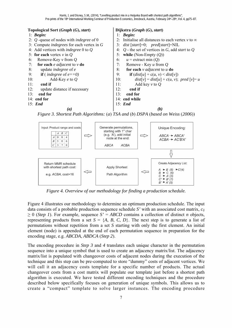
Table 2. Data representations derived from the cost matrix 4. Solution technique Here we present our methodology to identify the minimised costs and optimal sequence in the product wheel via a shortest path algorithm. We also compare the quality of the solutions obtained and computational performance of various shortest path algorithms and data structures. We show that all techniques find a unique optimum solution. The Topological Sort Algorithm (Figure 3(a)) visits vertices in the graph in the topological order. Initially, it computes the indegrees (number of incoming edges to a vertex) for each vertex in the graph. A vertex with the indegree of 0 is chosen as the first node to start a topological sort. If there is more than one vertex that has the indegree 0, then choose any one to be first in the topological order. All those vertices are added to the queue Q that stores the topological order of nodes to be visited. The main loop of the algorithm, removes each vertex from the queue, marks it as visited and updates the indegree information of each adjacent vertex (decrease by 1). If any updated vertex has indegree 0, it is added to the queue otherwise the distance of the path is updated. As a result of the main loop, the TSA “removes” vertices that do not have incoming edges. The “greedy” nature of the DSPA (Figure 3(b)) implies that at each stage, a search for the lowest value is extended until the destination node becomes reachable. The main loop starts searching from a source node (the current node), to all adjacent neighbours that have not been visited before in order to calculate distances to those nodes. The distance information is updated if it is less than any previously recorded value (which was set to infinity at initialisation). A node that is visited will not be considered in the search again and its distance is recorded as final with its lowest value. The next step is to select the next current (unvisited) node with the lowest distance, considering all its neighbours, and update distances if needed until the destination node has been reached.

In a Java application, for the DSPA implementation, we tested two data structures (the priority queue and pairing heaps) from the Weiss package (Weiss 2006). The priority queue is used to add a new node to the queue that contains information on the vertex and the distance when the total distance to that node is updated (when lower than a previous value). To select the next vertex, the minimum distance object is removed from the priority queue and algorithm continues until stopping condition is satisfied. The implementation of the pairing heap structure also integrates a priority queue concept that uses the distance as the ordering function where ordering property is re-established when update takes place.


7

Topological Sort (Graph (G), start) 1: Begin: 2: Q -queue of nodes with indegree of 0 3: Compute indegrees for each vertex in G 4: Add vertices with indegree 0 to Q 5: for each vertex v in Q 6: Remove-Key v from Q 7: for each e adjacent to v do 8: update indegree of e 9: if ( indegree of e==0) 10: Add-Key e to Q 11: end if 12: update distance if necessary 13: end for 14: end for 15: End

(a)

Dijkstra (Graph (G), start) 1: Begin: 2: Initialise all distances to each vertex v to ∞ 3: dist [start]=0; pred[start]=NIL 4: Q - the set of vertices in G, add start to Q 5: while (Non-Empty (Q)) 6: u = extract min (Q) 7: Remove - Key u from Q 8: for each v adjacent to u do 9: if (dist[u] + c(u, v) < dist[v]) 10: dist[v] = dist[u] + c(u, v); pred [v]= u 11: Add key v to Q 12: end if 13: end for 14: end while 15: End

(b) Figure 3. Shortest Path Algorithms: (a) TSA and (b) DSPA (based on Weiss (2006))

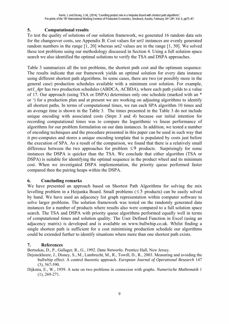
Figure 4. Overview of our methodology for finding a production schedule.

Figure 4 illustrates our methodology to determine an optimum production schedule. The input data consists of a probable production sequence schedule S’ with an associated cost matrix, cij

≥ 0 (Step 1). For example, sequence S’ = ABCD contains a collection of distinct n objects, representing products from a set S = {A, B, C, D}. The next step is to generate a list of permutations without repetition from a set S starting with only the first element. An initial element (node) is appended at the end of each permutation sequence in preparation for the encoding stage, e.g. ABCDA, ABDCA (Step 2).

The encoding procedure in Step 3 and 4 translates each unique character in the permutation sequence into a unique symbol that is used to create an adjacency matrix/list. The adjacency matrix/list is populated with changeover costs of adjacent nodes during the execution of the technique and this step can be pre-computed to store “dummy” costs of adjacent vertices. We will call it an adjacency costs template for a specific number of products. The actual changeover costs from a cost matrix will populate our template just before a shortest path algorithm is executed. We have tested different encoding techniques and the procedure described below specifically focuses on generation of unique symbols. This allows us to create a “compact” template to solve larger instances. The encoding procedure


8

No. of products

Data instance

Minimised cost

Shortest Path

Computational times (ms)**

TopologicalSort (TSA)

DSPA (priority queue)

DSPA (pairing

heap)

3 set1_3pr 16 ACBA 2.4 3.9 8.7

set2_3pr 21 ABCA 2.4 4.7 5.4

4 set1_4pr 17

ABDCA*+ 3.9 5.5 7

ACBDA

set2_4pr 45 ABDCA 1.7 3.1 6.4

5 set1_5pr 32 ADECBA 6.1 7.7 10.9

set2_5pr 121 ACEBDA 6.1 8.4 10.9

6

set1_6pr 37 AFCEBDA+

7.7 7.6 12.6 AEBCFDA*

set2_6pr 98

AFBCEDA+

4.7 9.7 10.9 AEFBCDA*+

AEFDCBA

7 set1_7pr 30

ADFGCBEA+ 24.3 28.5 51.7

ABCDFGEA*+

set2_7pr 60 ADBCEFGA 23.7 27.3 50.8

8 set1_8pr 23 AGDFCBHEA 81.2 75 93

set2_8pr 79 ABFCEDHGA 82.9 73.5 100.8

9 set1_9pr 34 AIHBCDEFGA 262.1 264.6 433.1

set2_9pr 62 ACBFIDGEHA 267.9 259.4 422.3

10 set1_10pr 36

AHBJCGFEDIA*+

2373.3 3087.1 5798.4 AHCFEJBGDIA

set2_10pr 80 ADJHFCEBIGA 2254.1 3486.3 5586.8 * solution determined by TSA + solution determined by DSPA(priority queue and/or pairing heap) ** average time for 10 runs(unique encoding/cost assignment excluded)

Table 3. Computational results compares character strings in the permutation sequence to decide whether or not that character string is unique. By unique we mean that a character has not yet appeared in that position of the wheel with the same set (without order) of proceeding characters. It transpires that we don’t need to consider the first character and the second and last character are trival. As way of an example, the permutation sequence ABCD, ABDC, ACBD, ACDB, ADBC, ADCB has the following unique encoding: ABCDD'C'C''B'D''B''D'''B'''C'''A'. As a result of unique encoding, four products will generate a list of 14 unique elements and for five products there are 34 unique elements. In the Step 5, the Shortest Path Algorithm (TSA or DSPA) is applied to the adjacency list/matrix representation and computes a shortest path cost from the start to the destination node and returns the associated path. Step 6, the shortest path is decoded to product representation and the optimal sequence in the Product Wheel is returned.


9

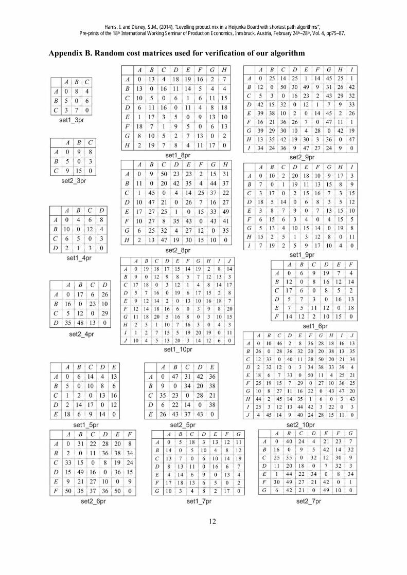
5. Computational results To test the quality of solutions of our solution framework, we generated 16 random data sets for the changeover costs, see Appendix B. Cost values for set1 instances are evenly generated random numbers in the range [1, 20] whereas set2 values are in the range [1, 50]. We solved these test problems using our methodology discussed in Section 4. Using a full solution space search we also identified the optimal solutions to verify the TSA and DSPA approaches.

Table 3 summarizes all the test problems, the shortest path cost and the optimum sequence. The results indicate that our framework yields an optimal solution for every data instance using different shortest path algorithms. In some cases, there are two (or possibly more in the general case) production schedules available with a minimum cost solution. For example, set1_4pr has two production schedules (ABDCA, ACBDA), where each path yields to a value of 17. Our approach (using TSA or DSPA) determines only one schedule (marked with an * or +) for a production plan and at present we are working on adjusting algorithms to identify all shortest paths. In terms of computational times, we run each SPA algorithm 10 times and an average time is shown in the Table 3. The times presented in the Table 3 do not include unique encoding with associated costs (Steps 3 and 4) because our initial intention for recording computational times was to compare the logarithmic vs linear performance of algorithms for our problem formulation on our data instances. In addition, we tested a number of encoding techniques and the procedure presented in this paper can be used in such way that it pre-computes and stores a unique encoding template that is populated by costs just before the execution of SPA. As a result of the comparison, we found that there is a relatively small difference between the two approaches for problem 9 products. Surprisingly for some instances the DSPA is quicker than the TSA. We conclude that either algorithm (TSA or DSPA) is suitable for identifying the optimal sequence in the product wheel and its minimum cost. When we investigated DSPA implementation, the priority queue performed faster compared then the pairing heaps within the DSPA. 6. Concluding remarks We have presented an approach based on Shortest Path Algorithms for solving the mix levelling problem in a Heijunka Board. Small problems ( 5 products) can be easily solved by hand. We have used an adjacency list graph representation within computer software to solve larger problems. The solution framework was tested on the randomly generated data instances for a number of products where results also were compared to a full solution space search. The TSA and DSPA with priority queue algorithms performed equally well in terms of computational times and solution quality. The User Defined Function in Excel (using an adjacency matrix) is developed and is available on www.bullwhip.co.uk. Whilst finding a single shortest path is sufficient for a cost minimising production schedule our algorithms could be extended further to identify situations where more than one shortest path exists. 7. References Bertsekas, D., P., Gallager, R., G., 1992. Data Networks. Prentice Hall, New Jersey. Dejonckheere, J., Disney, S., M., Lambrecht, M., R., Towill, D., R., 2003. Measuring and avoiding the

bullwhip effect: A control theoretic approach. European Journal of Operational Research 147 (3), 567-590.

Dijkstra, E., W., 1959. A note on two problems in connexion with graphs. Numerische Mathematik 1 (1), 269-271.


10

Disney, S., M., Hoshiko, L., Polley, L., Weigel, C., 2013. Removing bullwhip from Lexmark’s toner operations, Production and Operations Management Society Annual Conference, May 3rd-6th, Denver, USA.

Hedenstierna, C., P., T., Disney, S., M., 2012. Impact of scheduling frequency and shared capacity on production and inventory costs. Pre-prints of the 17th International Working Seminar of Production Economics, Innsbruck, Austria, February 20th -24th, 2, 277-288.

Hopcroft, J., Tarjan, R., 1973. Algorithm 447: Efficient algorithms for graph manipulation. Communications of ACM 16 (6), 372-378.

King, P.L., 2009. Lean for the Process Industries: Dealing with Complexity. CRC Press, Boca Raton, USA.

Ohno, T., 1998. Toyota Production System: Beyond Large-Scale Production, Productivity Press, Portland USA. ISBN 978-0-915299-14-0.

Salama, H., F., Reeves, D., S., Viniotis, Y. 1997. Evaluation of multicast routing algorithms for real-time communication on high-speed networks. IEEE Journal on Selected Areas in Communications 15 (3), 322-345.

Shingo, S., 1996. Quick Changeover for Operators: The SMED System, Productivity Press, Portland USA.

Weiss, M., A., 2006. Data structures & problem solving using Java. Addison-Wesley.


11

Appendix A. DAG’s for the 3-5 product wheel problem


12

Appendix B. Random cost matrices used for verification of our algorithm


13

Appendix C. VBA code for the Excel Add-In

TSA (adjArr):

Dim indegreeArr() As Integer Dim dist() As Integer Dim predecessors() As Integer Dim node As Integer Dim queueForIndeg As Collection Set queueForIndeg = New Collection ReDim dist(totCol) ReDim predecessors(totCol) ReDim indegreeArr(totCol) dist(1) = 0 For i = 2 To totCol dist(i) = 9999 Next i ' compute indegrees For i = 1 To totRow For j = 1 To totCol If adjArr(i, j) <> "‐1" Then indegreeArr(j) = indegreeArr(j) + 1 End If Next j Next i For i = 1 To totCol If indegreeArr(i) = 0 Then queueForIndeg.Add (i) End If Next i For i = 1 To queueForIndeg.Count If queueForIndeg.Count = 0 Then Exit For node = queueForIndeg.Item(CInt(i)) queueForIndeg.Remove (i) i = i ‐ 1 For j = 1 To totCol If adjArr(node, j) <> ‐1 Then indegreeArr(j) = indegreeArr(j) ‐ 1 If indegreeArr(j) = 0 Then queueForIndeg.Add (j) End If If (dist(node) + adjArr(node, j)) < dist(j) Then dist(j) = dist(node) + adjArr(node, j) predecessors(j) = node End If End If Next j Next i MsgBox "shortest distance cost= " & dist(totCol)

DSPA (adjArr):

Dim fromStr As Integer Dim dist() As Integer Dim closed() As Boolean Dim predecessors() As Integer Dim minDist As Integer Dim node As Integer ReDim dist(totCol) ReDim closed(totCol) ReDim predecessors(totCol) Dim queueForElem As Collection Set queueForElem = New Collection fromStr = 1 queueForElem.Add (CStr(fromStr)) predecessors(fromStr) = ‐1 dist(1) = 0 For i = 2 To strLenAdjArr dist(i) = 9999 Next i While queueForElem.Count <> 0 minDist = 9999 node = ‐1 For i = 1 To queueForElem.Count If dist(queueForElem.Item(i)) < minDist Then minDist = dist(queueForElem.Item(i)) node = queueForElem.Item(CInt(i)) End If Next i For i = 1 To queueForElem.Count If queueForElem.Item(i) = CStr(node) Then queueForElem.Remove (i) Exit For End If Next i closed(node) = True For i = 1 To totCol If adjArr(node, i) <> ‐1 Then If closed(i) = False Then If (dist(node) + adjArr(node, i)) < dist(i) Then dist(i) = dist(node) + adjArr(node, i) predecessors(i) = node queueForElem.Add (CStr(i)) End If End If End If Next i Wend MsgBox "shortest distance cost= " & dist(totCol)

Minimising Changeover Costs in the Heijunka Board with ... product mix in a Heijunka... · examples...

Documents

Transcript of Minimising Changeover Costs in the Heijunka Board with ... product mix in a Heijunka... · examples...