MINI-REPORT #2: PRELIMINARY DESIGN DOWNHOLE TURBINE FOR...

!

MINI-REPORT #2: PRELIMINARY DESIGN DOWNHOLE TURBINE FOR DRILLING

ENGI 8926: MECHANICAL DESIGN PROJECT II

GROUP 5

Bret Kenny 200902518

Chintan Sharma 200943512

Lida Liu 200814853

Piek Suan Saw 200829760

Revision Created by Date Reviewed

by Date Approved by Date

1 Group 5 3/7/14 Group 5 3/7/14 Dr. Yang

_ Pages

ENGI 8926: Mechanical Project II Mini-Report #2: Preliminary Design !

i!!

!Table of Contents

!1.0! Introduction ........................................................................................................... 1!

1.1! Project Background ..................................................................................... 1!1.2! Project Statement ......................................................................................... 1!1.3! Design Constraints ...................................................................................... 1!1.4! Design Methodology ................................................................................... 2!1.5! Working Philosophy .................................................................................... 2!

2.0! Theoretical Analysis .............................................................................................. 3!2.1! Blade Length ............................................................................................... 4!2.2! Blade Angles ............................................................................................... 6!2.3! Conclusion ................................................................................................... 7!

3.0! Computational Fluid Analysis ............................................................................... 8!3.1! Purpose ........................................................................................................ 8!3.2! Fluid Analysis Set-up and Assumptions ..................................................... 8!3.3! Turbine Power Curves ............................................................................... 10!3.4! Turbine Pressure Drop Curves .................................................................. 12!3.5! Conclusion ................................................................................................. 12!

4.0! Experimental Analysis ........................................................................................ 13!4.1! Purpose ...................................................................................................... 13!4.2! Apparatus .................................................................................................. 13!4.3! Design of Experiment ................................................................................ 13!4.4! Procedure ................................................................................................... 15!4.5! Data Acquisition ........................................................................................ 15!4.6! Analysis ..................................................................................................... 16!4.7! Conclusion ................................................................................................. 16!4.8! Recommendation ....................................................................................... 17!

5.0! Bibliography ........................................................................................................ 18!!


ii !

Figures

Figure 1: Downhole Turbine Assembly .............................................................................. 3!Figure 2: A- Top View of Rotor, B – Side View of Rotor and Stator Assembly ............... 3!

Figure 3: Output Power vs. Flow Rate (Blade Length Analysis) ....................................... 4!Figure 4: Power and Torque vs. Rotational Speed ............................................................. 5!

Figure 5: Pressure Drop versus Flow Rate (Blade Length Analysis) ................................. 5!Figure 6: Power Output and Pressure Drop versus Inlet Angle (Blade Angle Analysis) ... 6!

Figure 7 - Three Stage Rotor-Stator Assembly used for SolidWorks Flow Simulation (arrows showing flow directions) ............................................................................... 8!

Figure 8 – A. Flow streamlines in a three-stage stator-rotor assembly, B. Pressure profile across three-stage turbine ............................................................................................ 9!

Figure 9 - Turbine Power Curve from SolidWorks™ Flow Simulation .......................... 11!Figure 10 - Turbine Curve for Pressure Drops ................................................................. 12!

Figure 11 - Schematic diagram for experimental analysis ................................................ 14!Figure 12 - Photographs of the experimental setup .......................................................... 14!

Figure 13 - Set-up for data acquisition with RPM encoder and handing load of 1 kg ..... 15!Figure 14 - Power Curve Comparison between Theoretical, Computational and

Experimental Results ................................................................................................ 16!

!!

Appendices

APPENDIX A: BACKGROUND THEORY APPENDIX B: ROTOR AND STATOR GEOMETRY SELECTION APPENDIX C: PRELIMINARY DESIGN - DETAILED DRAWINGS APPENDIX D: COMPUTATIONAL FLUID DYANMICS SAMPLE CALCULATIONS !

!!!!!


1 !

1.0 Introduction 1.1 Project Background The design project undertaken by Group 5 for the ENGI 8926 course is in relation to research work being completed by the Advanced Drilling Group (ADG) in the engineering faculty at the Memorial University of Newfoundland (MUN). It has been identified by the ADG that within the drilling industry there is currently a space in the marketplace for a downhole assembly, which can provide mechanical rotational power to a variety of other downhole drilling tools. The design of a tool that can provide power to a range of downhole tools is the main objective of Group 5’s design project.

1.2 Project Statement Group 5 will design a downhole turbine assembly capable of delivering rotational mechanical energy to downhole drilling tools such as turbodrills, electrical generators, hydraulic motors, and a variety of other mechanical, electrical or hydraulic devices. The downhole turbine assembly design will be focused on providing the necessary output parameters to service other downhole tools. The design will use commercially available components and/or designs where applicable.

1.3 Design Constraints Downhole tools used during drilling operations must be designed with many factors in mind. These factors mainly arise from the conditions in which the tools must operate. Table 1 below highlights the major design constraints for the downhole turbine assembly to be designed by Group 5.

Table 1: Design Constraints

Constraint Description Size • Diameter = 4.0”

• Length ≈ 6.0’ Output • 600-800 RPM Input • Flow range = 150-300 gal/min

• ∆P < 300psi Strength (Axial, Compressive, and Torsional)

• Tool strength designed to API drill pipe specifications

Operational Conditions • Water-based drilling mud system Modular Design • Couple multiple turbine assemblies Cost • Minimize Health, Safety & Environment • Pressure build-up mitigation device,

compliance tool


2 !

1.4 Design Methodology This project will be completed in three main phases. The first phase: research and conceptual design is complete and included an initial comprehensive review of existing commercial and pre-commercial downhole turbines to develop an understanding of the configurations and variations between systems. In addition, the first phase involved a review of published scientific literature, product catalogues and technical manuals and guides, patent applications, and fluid mechanics analysis of turbine operation. The main result of the first phase was the selection a turbine type that is best suited to this application. The second phase of the project, which is presented in this report, includes the selection of the rotor and stator geometry (blade lengths and angles) and the number of turbine stages (rotor and stator pairs in series) through the use of theoretical analysis. Also completed in the second phase is the development of relationships between power output and pressure drop with respect to the number of turbine stages. Lastly, completed in this phase is an experimental analysis of a prototyped three stage turbine. The third and final project phase will involve the selection and design of additional turbine assembly components including the housing, bearings, drive shaft, etc. In addition, advanced flow testing will be completed to generate efficiency and flow, as well as power and turbine stage relationships. Lastly, the final phase will include system optimization and finalization of tool specifications.

1.5 Working Philosophy Figure 1 below displays a high-level CAD model of the downhole turbine assembly. The downhole turbine has a pipe-shaped housing with standard drill pipe connections at both ends. These connections allow for drill pipe and other downhole tools to be connected above and below the downhole turbine. The working mechanisms of the turbine are located within the housing. The main components are bearings, turbine stages (rotor and stator pairs), and a drive shaft. A gearbox/transmission is also shown in Figure 1, which will be considered to ensure shaft output speed or torque meets requirements. While the turbine assembly is in steady-state operation, drilling fluid enters the tool at the end of the tool labeled “inlet” in Figure 1. The flow passes through the inside of the housing and through passages in a bearing seating. This seating is used to support and centralize the bearings but still allow the passage of drilling fluid through the turbine assembly. The seating is attached to the housing to prevent any axial motion of the bearings. After flowing through the bearing seating, the flow will enter the staged turbine section which converts the flow’s kinetic energy into the desired rotational energy. The rotor and stator section consists of multiple stages. One stage contains one rotor and one stator. The stator is attached to the housing so it remains stationary, i.e. it does not rotate, for all time. The function of a stator is to turn the flow to a desired angle before contacting the rotor. This helps improve the efficiency of the turbine. The turned flow stream from the stator drives the rotor as it contacts the rotor blades. The rotor is mounted on the shaft, and thus the shaft rotates with the rotor. After the flow exits the rotor and stator section, it will pass through another bearing seating. At this point, the flow exits


3 !

through the bottom of the tool and continues to be circulated throughout the drilling mud system.

Figure 1: Downhole Turbine Assembly

2.0 Theoretical Analysis A theoretical analysis of the downhole turbine was completed with the objective of selecting the blade lengths and angles of the stator and rotor assembly (Figure 2). The theoretical analysis was completed prior to the computational and experimental analysis to gain a better understanding of the turbine’s performance before more detailed analysis was completed. Specifically, the stator and rotor blade lengths and angles were analyzed using Euler’s Turbomachinery equations and first principles. An overview of the equations used in this analysis is presented in Appendix A.

!Figure 2: A- Top View of Rotor, B – Side View of Rotor and Stator Assembly

The goal of selecting stator and rotor blade lengths and angles is to maximize power output while still satisfying all design constraints listed in Table 1. Both the blade length and blade angles influence the power output and pressure drop; therefore, the effect of both variables must be accounted coincidently for in the final turbine geometry selection.


4 !

The theoretical analysis was conducted in two parts. The first involves an analysis to develop relationships between turbine blade length and angles, and power output and pressure drop. The results of these analyses are presented below in Sections 2.1 and 2.2. The second part of the analysis involves the comparison of different workable turbine geometries with the design constraints in Table 1 to select a final geometry for the rotor and stator assembly. The result of the second phase of the theoretical analysis is presented in Section 2.3. Note: the results presented below in Sections 2.1 and 2.2 are for a single rotor a stator assembly.

2.1 Blade Length The blade length of the turbine is shown in Figure 2 above as the distance between the two arrows, which is also the annular space between the turbine’s inner and outer diameters. Equations A1 through A13 in Appendix A were used to determine the relationship between the turbine’s blade length, power output and pressure drop. To complete this analysis the outer diameter (Do) was held constant with a value of 4.0” (dictated by project constraint in Table 1) while the inner diameter (Di) was varied from 0.5” to 3.5” in 0.5” step increments. (That is, as the inner diameter increases the blade length decreases proportionally.) The required operating rotational speed of the turbine is within the range of 600-800 rpm. Therefore, iterations were completed for shaft speeds of 600, 700 and 800 rpm. The plots below display the relationship between power output versus flow rate and pressure drop versus flow rate for a variety of different inner diameter sizes. The data presented below is for shaft speeds of 600, 700 and 800 rpm and flow inlet and outlet angles of α=45° and β=135°, respectively (as shown in Figure 2 above).

!Figure 3: Output Power vs. Flow Rate (Blade Length Analysis)

The results presented in Figure 3 indicate, that for a given inner diameter, as flow rate is increased the output power increases. Specifically, substitution of all input equations into Equation 3A proves that the power output-increase is proportional to the square of the flow rate. In addition, as the inner diameter increases (blade length decreases) the


5 !

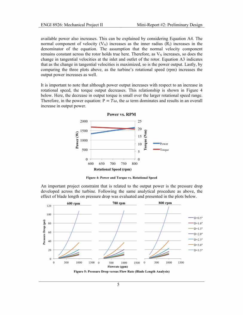
available power also increases. This can be explained by considering Equation A4. The normal component of velocity (VN) increases as the inner radius (Ri) increases in the denominator of the equation. The assumption that the normal velocity component remains constant across the rotor holds true here. Therefore, as VN increases, so does the change in tangential velocities at the inlet and outlet of the rotor. Equation A3 indicates that as the change in tangential velocities is maximized, so is the power output. Lastly, by comparing the three plots above, as the turbine’s rotational speed (rpm) increases the output power increases as well. It is important to note that although power output increases with respect to an increase in rotational speed, the torque output decreases. This relationship is shown in Figure 4 below. Here, the decrease in output torque is small over the larger rotational speed range. Therefore, in the power equation: Ρ = !", the ! term dominates and results in an overall increase in output power.

!Figure 4: Power and Torque vs. Rotational Speed

An important project constraint that is related to the output power is the pressure drop developed across the turbine. Following the same analytical procedure as above, the effect of blade length on pressure drop was evaluated and presented in the plots below.

!Figure 5: Pressure Drop versus Flow Rate (Blade Length Analysis)


6 !

The relationship between flow rate and pressure drop are almost identical to the relationship between flow rate and power shown above. This is due to the relationship between the two values expressed in Equation A13.

2.2 Blade Angles The blade angles of the turbine are shown in Figure 2 above as angles α and β, or the inlet and outlet angles. To complete the analysis, three angles were considered for β: 100°, 135° and 170°, and for each case the relationship between output power and inlet angle α was developed. Various iterations were completed holding the value of β constant while α was varied. This process was completed for rotational speeds of 600, 700 and 800 rpm and for the same inner diameter range presented in the blade length analysis above. The plot below displays the relationship between power output and angle α for three β angles. Note the results shown in Figure 6 below are for the following operating conditions: 500gpm, 600rpm, Di=3.0".

!

Figure 6: Power Output and Pressure Drop versus Inlet Angle (Blade Angle Analysis)

Figure 6 above shows that with a constant outlet angle β, as α decreases the output power increases. In addition, with constant angle α, as β increases, the output power greatly increases. Therefore, to maximize output power, it is best to have a very small angle α (approaching 0) and a very large angle β (approaching 180). However, although maximum power output is desired, the pressure drop per stage sharply increases at inlet angles less than 40°.


7 !

2.3 Conclusion The results from the analyses presented above were used to determine a range of workable blade length and angle combinations from which the final turbine geometry could be chosen. These solutions were then compared with the design constraints in Table 1 as well as other design guidelines and assumptions including:

• Stage length: Lstage = 3.0 inches • 25° ≤ α ≤ 45° and 100° ≤ β ≤ 135° • Efficiency (η) ≈ 25 %

These parameters were assumed for the selection of the final turbine geometry to result in a conservative design. The development of possible solutions was based on satisfying the above criteria in addition to maximizing power output. First, considering the blade length, it is shown in Figure 3 above that output power increases as inner diameter increases. Therefore, the largest three inner diameters (3.5”, 3.0” and 2.5”) were considered for the selection of final blade length. Second, several α and β angle combinations were considered for each diameter. A list of all the considered turbine geometry combinations is shown in Appendix B. The solution that was selected to proceed for further computational and analytical analysis satisfies all design constraints and maximizes output power. The selected turbine geometry has an outer and inner diameters of 4.0” and 3.0” respectively (i.e. blade length of 0.5”), α = 45°, and β = 135°. The selected dimensions are relatively conservative compared to the other considered cases. The expected pressure drop per stage is 12.37psi, which will require 24 stages (rotor and stator pairs) and measure approximately 6.06ft long. Detailed drawings of the selected rotor and stator dimensions are attached in Appendix C.


8 !

3.0 Computational Fluid Analysis 3.1 Purpose Computational fluid dynamics analysis was completed using the turbine geometry selected in the theoretical analysis in Section 2. The main reason for conducting computation fluid analysis was to verify and evaluate the following design parameters: 1. Compare and verify the results from:

a. Theoretical power and flow curves (Figures 3 and 5) b. Data acquired from experimental analysis

2. Develop relationships between: a. Output power and turbine stages b. Pressure drop and turbine stages

3.2 Fluid Analysis Set-up and Assumptions The SolidWorks™ Flow Simulation intuitive CFD (Computational Fluid Dynamics) tool was used to simulate liquid flow through the rotor-stator assembly. Figure 7 below illustrates the outlined view of three stages of the rotor – stator assembly with inlet and outlet flow directions that were used to conduct the fluid analysis. Further, Figure 8 A and B show the trajectories of the fluid streamlines as well as the pressure profile in the three-stage turbine assembly. The pressure profile across the three-stage turbine decreases from the inlet to the outlet (from left to right). Expected pressures within the turbine are presented for a flow rate of 200 GPM in Appendix D.

!

Figure 7 - Three Stage Rotor-Stator Assembly used for SolidWorks Flow Simulation (arrows showing flow directions)


9 !

!

!Figure 8 – A. Flow streamlines in a three-stage stator-rotor assembly, B. Pressure profile across

three-stage turbine

The CFD software was used to simulate liquid flow in different scenarios and analyze the turbine’s performance, including parameters such as velocity and related pressure drop. For the purpose of the analysis, the following inputs were considered:

Table 2 - Input parameters for SolidWorks Flow Simulation

Parameter Value Flow Rates 10 GPM to 800 GPM

Turbine Stages 1, 3, 5, 10, and 50 Fluid Properties Water, ρ = 1000 kg/m3

Pressure 101,325 Pa (1 atm) Temperature 293.2 K Turbulence

(Default Values) Turbulence Intensity (2%)

Turbulence Length (0.0010414 m)


10 !

In addition to the input parameter outlined in Table 2, the following assumptions were made to conduct the fluid analysis:

• Cavities without flow conditions were excluded to disregard closed internal spaces not involved in the analysis

• Adiabatic wall condition was assumed, denoting heat-insulated walls • Minimum gap size between rotor and stator was set at 0.004 m and rotor and

stator blades were assumed to be 0.002m thick • Flow regime was set to laminar internal flow throughout the turbine section

3.3 Turbine Power Curves The results from the SolidWorks™ Flow Simulation provided values for differential pressures and flow velocities at the inlet and outlet of the turbine for 1, 3, 5, 10, and 50 turbine stages. From these values, the overall power and pressure drop across the entire assembly was evaluated using mechanical energy balance equations 1 and 2 below. !!!!! +

!!!" =

!!!!! +

!!!" +!! [1]

!! = (!!

!

!! −!!!!!)+ (

!!!" −

!!!") [2]

Where: !!= Fluid Density V1 =Inlet velocity !!= Inlet Pressure V2 = Outlet velocity !!= Outlet Pressure !! = Work done by Turbine !!= Acceleration due to gravity Equations 1 and 2 were used to determine the power generated by turbine for 1, 3, 5, 10, and 50 turbine stages arrangements. The power generated by the turbine was computed for flow rates ranging from 10 GPM to 400GPM. Figure 9 below show the results from the flow simulation on a plot of Power vs. Flow Rate.


11 !

Figure 9 - Turbine Power Curve from SolidWorks™ Flow Simulation

Three major conclusions can be made from the results in Figure 9 to understand the relationship between output power, flow rates and turbine stages: 1. Flow Rate < 30 GPM

At flow rates below 30 GPM, no power output is produced. This shows that inlet source should provide atleast 30 GPM of fluid to turn the rotor of the turbine unit. The turbine start-up flow rate required for the turbine to start operating increases with number of stages. For instance, flow rate must be greater than 175 GPM for a 50 stage turbine unit.

2. 30 GPM < Flow Rate < 200 GPM At flow rates between 30 GPM and 200 GPM, power is weakly dependent on the number of stages of the turbine i.e. minor increase in power is observed while increasing the number of turbine stage.

3. Flow Rate > 200 GPM At flow rates greater than 200 GPM, power is stongly dependent on the number of stages of the turbine. For instance, at 350 GPM moving from 1 stage turbine to 3 stage turbine increases the output power from 1 kW to 2 kW.

From these three conditons, it can be concluded that operating at higher flow rates (>200 GPM) will require lesser number of stages to generate same amout of output power.


12 !

3.4 Turbine Pressure Drop Curves Similar to the turbine power analysis, the pressure data from SolidWorks™ Flow Simulation was evaluated to analyze the pressure drop across the turbine unit for 1, 3, 5, 10, and 50 turbine stages. Figure 10 below plots the results of SolidWorks™ Flow Simulation that shows the relationship between the pressure drop, number of turbine stages, and flow rates.

Figure 10 - Turbine Curve for Pressure Drops

From the plot, it can be noted that by increasing the number of turbine stages the pressure drop also increases across the inlet and outlet of the turbine unit. Similary, operating at higher flow rates results in higher pressure drop. The pressure drop design constraint is equal to 300psi and is highlighted in Figure 10.

3.5 Conclusion In conclusion, the results from Computational Fluid Analysis were used to calculate theoretical power and flow curves. The computational results further validate the results achieved in the theoretical design phase and a comparison is shown below in Figure 14. In addition, CFD analysis was used to provide power, pressure and flow relationships that will be evaluated in the selection of the number of stages for the turbine. Maximizing the output power will require higher flow rates and will result in larger pressure drop. In terms of the number of stages, increasing the number of stages will increase the output power but will also result in higher pressure drop. Hence, the design of overall turbine unit will be optimized to meet the design constraints of the project.

Design Constraints of 300 psi


13 !

4.0 Experimental Analysis 4.1 Purpose The main purpose of conducting experimental analysis was to evaluate the performance of the downhole turbine assembly prototype. The prototype was modeled after the selected turbine geometry from the theoretical and computational analyses. The experiment was conducted by measuring the rotational speeds and torques at different flow rates. The experimental data was used to calculate the power output and compared to the theoretical and computational power output.

4.2 Apparatus Following materials were used to conduct the experiment:

Table&3:&Experiment&Setup&Supplies&

Item Description 1 Rotor and Stator fabricated using Rapid Prototype Machine 2 2” Male ABS Pipe Connection 3 2” ID ABS Pipe 4 2” – 90 Degree ABS Pipe Elbow 5 2”x4” ABS Pipe Crossover 6 4” ID ABS Pipe 7 Perforated ABS Pipe End Cap 8 0.5” Aluminum Shaft 9 RPM Encoder (Tachometer) 10 1 kg load to apply torque

4.3 Design of Experiment The laboratory exercise was set up in the fluids laboratory facility at the Memorial University of Newfoundland. Figure 11 outlines the schematic diagram of the experimental set-up. The flow source was a 2-in Female NPT pipe, controlled by a manually operated valve. A series of pipe fittings, pipes, an elbow, and a reducer were used to guide the flow from the pipe inlet to the outlet where the flow drained into the deep water tank. The turbine assembly along with aluminum shaft was placed inside the 4” ABS pipe. Figure 12 shows actual photographs of the experimental apparatus.


14 !

!Figure 11 - Schematic diagram for experimental analysis

Figure 12 - Photographs of the experimental setup

The flow for the experiment was initiated through use of a hand-operated valve upstream of the 2” ABS pipe. Once initiated, time was allotted to allow the system to develop steady-state flow conditions. The experiment used a total of four flow rates to gather data. The data acquisition was performed as illustrated in Figure 13. The shaft was extended outside the 4” ABS pipe and a reflective marker was used provide feedback to the encoder. A 1 kg weight was tied to the end of the shaft using a 2 m piece of string for determining the output torque. The flow rate was measured by recording the time required to fill a 4-gallon bucket.


15 !

!!

Figure 13 - Set-up for data acquisition with RPM encoder and handing load of 1 kg

4.4 Procedure To following procedure was implemented to successfully conduct the laboratory exercise:

1. Attach the hanging weight to the apparatus to ensure it is at its lowest position 2. Turn the valve handle to the first position (first flow rate) 3. Wait approximately 5 seconds to allow the flow to develop steady-state

conditions 4. Let the shaft rotate freely and measure the rotational speed with the encoder 5. When the weight reaches maximum height near the shaft, close the valve 6. Repeat steps 1 to 5 three more times to obtain 4 sets of data for each flow rate

4.5 Data Acquisition The data recorded during the laboratory exercise is displayed in Table 4 below. It is evident from this data that as the flow rate increases, the shaft speed and therefore output power also increase.

Table 4 - Experimental Data

Valve Position

Flow Rate (GPM)

Shaft Speed (RPM)

Torque (Nm) (Load of 1 Kg)

Calculated Power (W)

(Torque * ω) 1 45 175 0.058 0.9 2 56 260 0.058 1.4 3 71 330 0.058 1.8 4 87 525 0.058 2.8


16 !

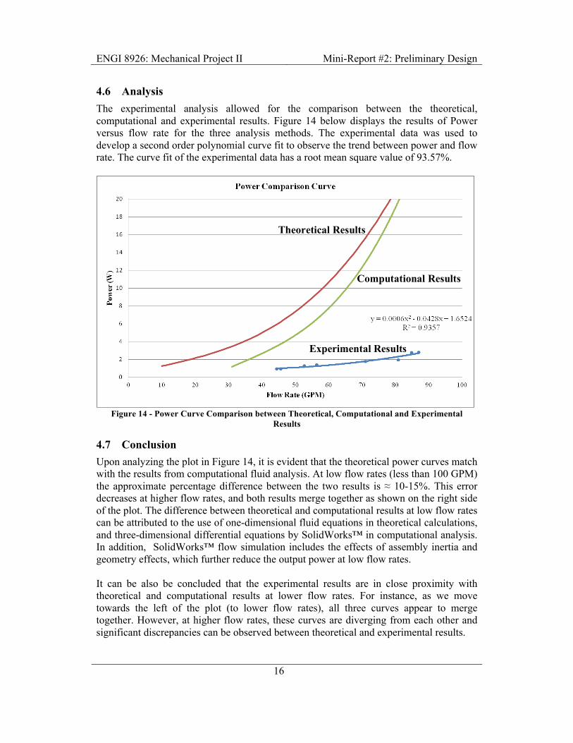
4.6 Analysis The experimental analysis allowed for the comparison between the theoretical, computational and experimental results. Figure 14 below displays the results of Power versus flow rate for the three analysis methods. The experimental data was used to develop a second order polynomial curve fit to observe the trend between power and flow rate. The curve fit of the experimental data has a root mean square value of 93.57%.

!Figure 14 - Power Curve Comparison between Theoretical, Computational and Experimental

Results

4.7 Conclusion Upon analyzing the plot in Figure 14, it is evident that the theoretical power curves match with the results from computational fluid analysis. At low flow rates (less than 100 GPM) the approximate percentage difference between the two results is ≈ 10-15%. This error decreases at higher flow rates, and both results merge together as shown on the right side of the plot. The difference between theoretical and computational results at low flow rates can be attributed to the use of one-dimensional fluid equations in theoretical calculations, and three-dimensional differential equations by SolidWorks™ in computational analysis. In addition, SolidWorks™ flow simulation includes the effects of assembly inertia and geometry effects, which further reduce the output power at low flow rates. It can be also be concluded that the experimental results are in close proximity with theoretical and computational results at lower flow rates. For instance, as we move towards the left of the plot (to lower flow rates), all three curves appear to merge together. However, at higher flow rates, these curves are diverging from each other and significant discrepancies can be observed between theoretical and experimental results.

Experimental Results

Computational Results

Theoretical Results


17 !

4.8 Recommendation Advanced Experimental Analysis It is recommended to conduct an advanced experimental analysis to analyze the turbine’s operation at higher flow rates. For this purpose, the drilling rig provided by the Advanced Drilling Group will be used to connect the three-stage turbine unit to high power pumps. These pumps can provide flow rates up to 200 GPM. Besides high flow rates, the experimentation setup will allow the team to connect electronic pressure gauge to achieve accurate pressure drops across the turbine unit. From the acquired flow rates, pressure drop, torque, and rotational speed, it will possible to calculate the overall efficiency of the turbine unit. The experiment will further assist the team to compute relationships between turbine efficiency, flow rates, and number of stages. Furthermore, the experimental setup will allow the application of higher loads to the turbine to measure the stalling torque values. Computational Fluid Analysis using Ansys Dynamic Suite The computational fluid analysis for the turbine can be conducted using Ansys Dynamic Suite. The software provides a finer mesh size, and incorporates dynamic turbine conditions. Ansys can provide dynamic values for torque generated, and rotation speed of the turbine at a given flow rate. This will assist the team to generate computational efficiency curves and compare the results with the advanced experimental analysis.

!!!!!!!!!!!!!!!!!!!!!!


18 !

5.0 Bibliography Hinchey,!M.!(2014).!Fluid&Power&Machines.!Retrieved!02!20,!2014,!from!ENGR!6961:!Fluid!Mechanics!II:!http://www.engr.mun.ca/~hinch/6961/NOTES/POWER.pdf!!Pritchard,!P.!J.,!&!Leylegian,!J.!C.!(2011).!Fox&and&McDonald's&Introduction&to&Fluid&Mechanics.!Hoboken,!New!Jersey,!USA:!John!Wiley!&!Sons.!!

!!!!!!!!!!!!!!!!!!!!


A1 !

!!!!!!!!!!!!!!!!!!!

APPENDIX A: BACKGROUND THEORY !!!!!!!!!!!!!!!!!!!!!!


A2 !

!Euler’s Turbomachinery Equations The Euler Turbomachinery equations were developed to analyze fluid interaction with machines such as pumps and turbines and therefore apply to machines both doing work on and extracting work from a fluid flow. Euler’s equations are based on the angular momentum principle. According to (Pritchard & Leylegian, 2011), when the angular momentum principal is applied to a control volume the result is:

!!×!!! + !!"

!×!!!"# + !!!!"# =!!" !

!"!×!!!"# + ! !!×!!!"! ∙ !!

!" [A1]

Where:

!!!= Radius !! = Surface forces ! = Gravity ρ = Density V = Fluid volume inside turbine !!!!"#!= Shaft torque

!= Velocity !! = Surface area Equation A1 indicates, “that the moment of surface forces and body forces, plus the applied torque, lead to a change in the angular momentum of the flow.” (Pritchard & Leylegian, 2011) Here, the surface forces are caused by friction and pressure, while the body forces are caused by gravity and applied torque, which will be positive in the case of a turbine. Equation A1 is further simplified for the case of turbine analysis resulting in the following scalar equations for shaft torque and power: !!!!"# = !"#!! !" − !"#!! !"# [A2] !"#$% = !"#!!! !" − !"#!!! !"# = !"!!!! !" − !"!!!! !"# [A3] Where:

R = Radius ρ = Density Q = Flow rate !!= Tangential velocity !!= Rotational speed !!= Velocity of turbine at radius R Equations A2 and A3 above evaluate the changes in angular momentum at the inlet and outlet of a turbine to determine torque and power. The tangential momentum at the inlet and outlet is equal to !"!! and is the only momentum component that causes rotation about the shaft axis. Multiplying the momentum change by a moment arm R, provides torque. Furthermore, multiplying torque by rotational speed ! provides power. (Hinchey, 2014) Considering the above equations, it is necessary to determine the tangential velocity and turbine velocity in order to calculate the system torque and power. First, the tangential velocities can be determined by using velocity diagrams to develop a general expression. Figure A1 below indicates the velocity vectors at the inlet and outlet of the turbine stator (stationary vanes) and rotor (rotating element connected to shaft). It is evident from this


A3 !

figure that the fluid flows into the stator (V1) at an angle parallel to the shaft and exits at an angle α. The fluid exiting the stator (V2) at angle α contacts the rotor blades, which cause the flow to turn in a direction parallel to the blade. The flow continues downward through the rotor and exits at angle β with velocity V3. (Hinchey, 2014)

!Figure A 1: Rotor and Stator Velocity Diagram

To calculate V1 the following equation is used:

!! =!

!(!!! − !!!)= !!! [A4]

Where:

Q = Flow rate ro = Outer radius ri = Inner radius !! = Normal velocity Equation A4 requires that the flow rate through the turbine is known and the denominator of the equation represents the flow area of the turbine. That is, the annular area between the shaft and housing. After passing through the stator, the velocity of the flow has changed. Particularly, the tangential component of the flow has increased and the normal component is assumed to remain constant. Therefore, the resulting velocity !! also increases. The net velocity magnitude!!! and its tangential component V2t can be calculated using the following formulas. (Hinchey, 2014)

!! =!!sin! [A5]

!!! = !! cot! [A6] The tangential velocity V2t in Equation 6 is equal to the inlet tangential velocity to the rotor in Equation A3.


A4 !

Next, consider the flow exiting the rotor. Similar to the stator, the flow has changed velocity with respect to both magnitude and direction. Again at this point, the normal velocity is considered to be constant throughout the turbine, with the net velocity changing due to changes in the tangential component. Therefore, to calculate the velocity V3 and tangential velocity V3t, the following equations can be used. (Hinchey, 2014)

!! =!!!cos! [A7]

!!! = !! cot! + !! [A8] !! = !!"! [A9] Where: !!" = ! (!!!!!)!

Note: β is measured counter clockwise from the horizontal The tangential velocity !!! in Equation A8 is equal to the outlet tangential velocity in Equation A3. In addition, VB (turbine speed) in Equation A9 is a function of the average turbine radius and the rotational speed of the turbine. Here, the rotational speed must be assumed or a range must be selected to determine its effect on tangential velocity and thus, output power/torque. Equations A4 through A9 can be used to determine all the inputs for Equations A2 and A3 to calculate theoretical output torque and power of the turbine. Mechanical Energy Balance In addition to calculating the output power of the turbine, a major constraint of the downhole turbine assembly design is the differential pressure drop across the tool. Specifically, the pressure drop across the turbine assembly cannot exceed 300psi. Therefore, it is necessary to evaluate the pressure drop across the stator and rotor as they are responsible for the majority of the pressure loss within the tool. First, consider the pressure drop across the stator. Conservation of energy results in the following equation:

!!!!2 +!ℎ! +!! = !!!!

2 +!ℎ! +!! [A10]

Where: ! = Mass flow rate V1 Inlet velocity ℎ!= Inlet enthalpy V2 = Outlet velocity ℎ!= Outlet enthalpy !!= Work input !! = Work output


A5 !

Equation A10 equates the flow’s kinetic and pressure energy at the inlet and outlet of the stator and accounts for any work added or removed from the flow as it passes through the stator. The stator always remains stationary; therefore, no work is added or removed from the flow (!! and !! = 0). The stator’s main purpose is to increase the flow’s kinetic energy from inlet to outlet. A transfer of pressure energy to kinetic energy and thus a decrease in the flow’s pressure energy accomplishes this. (Hinchey, 2014) Using the following substitutions, Equation 10 can be further simplified resulting in the following solution for the pressure drop across the stator:

ℎ = ! + !" = !" + !! !→ ℎ ≈ !! !(!"#$"%&!!"#$. !ℎ!"#$%) [A11]

!!!2 + !!! = !!!

2 + !!! !→ !!! − !! = Δ! = ! !!! − !!!2 [A12]

Equation A11 indicates that there will be little change in the fluid temperature across the stator; therefore, the temperature term in the expression for enthalpy can be neglected and enthalpy becomes a function of pressure and density only. V1 and V2 in Equation 12 can be calculated using Equations A4 and A5. Following a similar process it can be proven that the pressure drop across the rotor can be expressed as the following:

Δ! =!!! [A13]

Where:

!! = !!!!"#×! = Turbine power output Q = Flow rate Therefore, the amount of output turbine power is directly proportional to the pressure drop across the rotor. To determine the total pressure drop across both the rotor and stator, the respective pressure drops calculated in Equations A12 and A13 are summed together. !!!!!!!!!!!


B1 !

!!!!!!!!!!!!!!!!!!

APPENDIX B: ROTOR AND STATOR GEOMETRY SELECTION

!!!!!!!!!!!!!!!!!!!!!!!


B2 !

The table below lists the turbine geometries that were considered in the final selection process. The data in the table below is for a rotational speed of 600rpm and a flow rate of 200gpm. Lastly, note that the number of stages and length of the turbine in the table below were calculated based on the assumption of a 300psi total pressure drop and that the pressure drop per stage is linear along the length of the turbine. The final turbine geometry selection is highlighted below.

!Table B 1: List of Potential Turbine Geometries

!!!!!!!!!!!!!!!!!!!


C1 !

APPENDIX C: PRELIMINARY DESIGN - DETAILED DRAWINGS

!!!!!!!!!!!!!!!!!!

� ��

� ��

� ��

��

��

�� $

$

6(&7,21�$�$�;� ��

52725

:(,*+7��

$�

6+((7��2)��6&$/(��

':*�12�

7,7/(�

5(9,6,21'2�127�6&$/(�'5$:,1*

0$7(5,$/�

'$7(6,*1$785(1$0(

'(%85�$1'�%5($.�6+$53�('*(6

),1,6+�81/(66�27+(5:,6(�63(&,),('�',0(16,216�$5(�,1�0,//,0(7(56685)$&(�),1,6+�72/(5$1&(6��/,1($5��$1*8/$5�

4�$

0)*

$339'

&+.'

'5$:1

3$57��B52725

1. For experimentation purposes, rotor was attached to output shaft using set screws. Final design on the connection method between rotor and shaft will be conducted in the next analysis phase

2. The blade thickness was assumed to be 2mm (rapid prototyping constraint). However, final design blade thickness will be determined from FEA in the next analysis phase.

� ��

� ��

� ��

� ��

��

��

��

$

$

��

��

��

6(&7,21�$�$

3$57��B67$725

//

:(,*+7��

$�

6+((7��2)��6&$/(��

':*�12�

7,7/(�

5(9,6,21'2�127�6&$/(�'5$:,1*

0$7(5,$/�

'$7(6,*1$785(1$0(

'(%85�$1'�%5($.�6+$53�('*(6

),1,6+�81/(66�27+(5:,6(�63(&,),('�',0(16,216�$5(�,1�0,//,0(7(56685)$&(�),1,6+�72/(5$1&(6��/,1($5��$1*8/$5�

4�$

0)*

$339'

&+.'

'5$:1

67$725

� �� ; �

� ��

��

��

� � ��

��;��

,7(0�12� 1DPH 47<�

� 5RWRU �

� 6KDIW �

� 6WDWRU �� %DOO�%HDULQJ �

� +RXVLQJ �

� &DS �

��67$*(�$66(0%/<

:(,*+7��

$�

6+((7��2)��6&$/(��

':*�12�

7,7/(�

5(9,6,21'2�127�6&$/(�'5$:,1*

0$7(5,$/�

'$7(6,*1$785(1$0(

'(%85�$1'�%5($.�6+$53�('*(6

),1,6+�81/(66�27+(5:,6(�63(&,),('�',0(16,216�$5(�,1�0,//,0(7(56685)$&(�),1,6+�72/(5$1&(6��/,1($5��$1*8/$5�

4�$

0)*

$339'

&+.'

'5$:1

$66(0%/<��B�67$*(


D1 !

APPENDIX D: COMPUTATIONAL FLUID DYANMICS SAMPLE CALCULATIONS

!!!!!!!!!!!!!!!!!!!!!!


D2 !

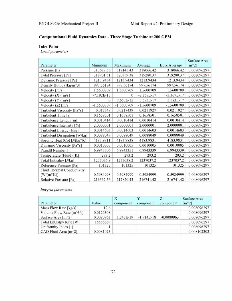
Computational Fluid Dynamics Data - Three Stage Turbine at 200 GPM Inlet Point Local parameters

Parameter Minimum Maximum Average Bulk Average

Surface Area [m^2]

Pressure [Pa] 317687.56 319145.43 318066.42 318066.42 0.008096297 Total Pressure [Pa] 318901.51 320359.38 319280.37 319280.37 0.008096297 Dynamic Pressure [Pa] 1213.9434 1213.9434 1213.9434 1213.9434 0.008096297 Density (Fluid) [kg/m^3] 997.56174 997.56174 997.56174 997.56174 0.008096297 Velocity [m/s] 1.5600709 1.5600709 1.5600709 1.5600709 0.008096297 Velocity (X) [m/s] -7.192E-15 0 -3.367E-17 -3.367E-17 0.008096297 Velocity (Y) [m/s] 0 7.653E-15 3.583E-17 3.583E-17 0.008096297 Velocity (Z) [m/s] -1.5600709 -1.5600709 -1.5600709 -1.5600709 0.008096297 Turbulent Viscosity [Pa*s] 0.017348 0.0217439 0.0211927 0.0211927 0.008096297 Turbulent Time [s] 0.1658501 0.1658501 0.1658501 0.1658501 0.008096297 Turbulence Length [m] 0.0010414 0.0010414 0.0010414 0.0010414 0.008096297 Turbulence Intensity [%] 2.0000001 2.0000001 2.0000001 2.0000001 0.008096297 Turbulent Energy [J/kg] 0.0014603 0.0014603 0.0014603 0.0014603 0.008096297 Turbulent Dissipation [W/kg] 0.0088049 0.0088049 0.0088049 0.0088049 0.008096297 Specific Heat (Cp) [J/(kg*K)] 4183.9811 4183.9838 4183.9831 4183.9831 0.008096297 Dynamic Viscosity [Pa*s] 0.0010005 0.0010005 0.0010005 0.0010005 0.008096297 Prandtl Number [ ] 6.9943306 6.9943351 6.9943339 6.9943339 0.008096297 Temperature (Fluid) [K] 293.2 293.2 293.2 293.2 0.008096297 Total Enthalpy [J/kg] 1237036.9 1237038.2 1237037.2 1237037.2 0.008096297 Reference Pressure [Pa] 101325 101325 101325 101325 0.008096297 Fluid Thermal Conductivity [W/(m*K)] 0.5984998 0.5984999 0.5984999 0.5984999 0.008096297 Relative Pressure [Pa] 216362.56 217820.43 216741.42 216741.42 0.008096297 !Integral parameters

Parameter Value

X-component

Y-component

Z-component

Surface Area [m^2]

Mass Flow Rate [kg/s] 12.6 0.008096297 Volume Flow Rate [m^3/s] 0.0126308 0.008096297 Surface Area [m^2] 0.0080963 1.247E-19 -1.914E-18 -0.0080963 0.008096297 Total Enthalpy Rate [W] 15586669 0.008096297 Uniformity Index [ ] 1 0.008096297 CAD Fluid Area [m^2] 0.0081023 0.008102303 !!!!!!


D3 !

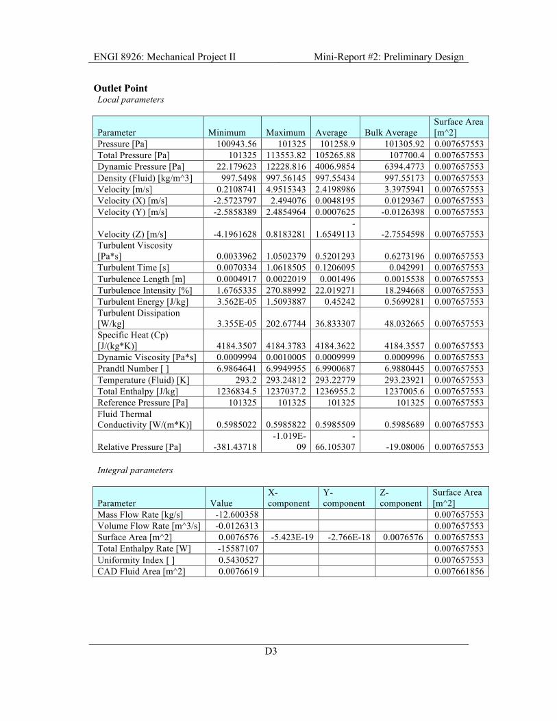
Outlet Point Local parameters

Parameter Minimum Maximum Average Bulk Average

Surface Area [m^2]

Pressure [Pa] 100943.56 101325 101258.9 101305.92 0.007657553 Total Pressure [Pa] 101325 113553.82 105265.88 107700.4 0.007657553 Dynamic Pressure [Pa] 22.179623 12228.816 4006.9854 6394.4773 0.007657553 Density (Fluid) [kg/m^3] 997.5498 997.56145 997.55434 997.55173 0.007657553 Velocity [m/s] 0.2108741 4.9515343 2.4198986 3.3975941 0.007657553 Velocity (X) [m/s] -2.5723797 2.494076 0.0048195 0.0129367 0.007657553 Velocity (Y) [m/s] -2.5858389 2.4854964 0.0007625 -0.0126398 0.007657553

Velocity (Z) [m/s] -4.1961628 0.8183281 -

1.6549113 -2.7554598 0.007657553 Turbulent Viscosity [Pa*s] 0.0033962 1.0502379 0.5201293 0.6273196 0.007657553 Turbulent Time [s] 0.0070334 1.0618505 0.1206095 0.042991 0.007657553 Turbulence Length [m] 0.0004917 0.0022019 0.001496 0.0015538 0.007657553 Turbulence Intensity [%] 1.6765335 270.88992 22.019271 18.294668 0.007657553 Turbulent Energy [J/kg] 3.562E-05 1.5093887 0.45242 0.5699281 0.007657553 Turbulent Dissipation [W/kg] 3.355E-05 202.67744 36.833307 48.032665 0.007657553 Specific Heat (Cp) [J/(kg*K)] 4184.3507 4184.3783 4184.3622 4184.3557 0.007657553 Dynamic Viscosity [Pa*s] 0.0009994 0.0010005 0.0009999 0.0009996 0.007657553 Prandtl Number [ ] 6.9864641 6.9949955 6.9900687 6.9880445 0.007657553 Temperature (Fluid) [K] 293.2 293.24812 293.22779 293.23921 0.007657553 Total Enthalpy [J/kg] 1236834.5 1237037.2 1236955.2 1237005.6 0.007657553 Reference Pressure [Pa] 101325 101325 101325 101325 0.007657553 Fluid Thermal Conductivity [W/(m*K)] 0.5985022 0.5985822 0.5985509 0.5985689 0.007657553

Relative Pressure [Pa] -381.43718 -1.019E-

09 -

66.105307 -19.08006 0.007657553 !Integral parameters

Parameter Value

X-component

Y-component

Z-component

Surface Area [m^2]

Mass Flow Rate [kg/s] -12.600358 0.007657553 Volume Flow Rate [m^3/s] -0.0126313 0.007657553 Surface Area [m^2] 0.0076576 -5.423E-19 -2.766E-18 0.0076576 0.007657553 Total Enthalpy Rate [W] -15587107 0.007657553 Uniformity Index [ ] 0.5430527 0.007657553 CAD Fluid Area [m^2] 0.0076619 0.007661856 !!!

MINI-REPORT #2: PRELIMINARY DESIGN DOWNHOLE TURBINE FOR...

Documents

Transcript of MINI-REPORT #2: PRELIMINARY DESIGN DOWNHOLE TURBINE FOR...