MIMO Channels and Space-Time Coding - pudn.comread.pudn.com/downloads111/doc/comm/464263/MIMO...

MIMO Channels

and Space-Time Coding

Presenters: Christian Schlegel and Zachary [email protected]; [email protected]

WOC 2002, Tutorial PresenationBanff, AB, CANADA, July, 2002

Outline:

• Capacity of MIMO Channels: We discuss the information theo-retic bases for the capacity arguments of MIMO channels and presentfundamental results and methods.• Channel Modeling and Realizable Capacity: We discuss sim-

ple ray-tracing channel models and study the capacity of these ar-tificially generated channels. Basic conclusions on the behavior ofreal-world MIMO channels are drawn.• Space-Time Coding: We introduce the basics of space-time coding

and modulation methods, such as orthogonal designs, unitary space-time codes, group space-time codes. We discuss error performancemeasures, and optimal and sub-optimal decoding algorithms.• Space-Time Communications Systems: We discuss basic layer-

ing methods and the addition of error control coding to space-timesystems. We show how complex decoders work and how they per-form.

MIMO CHANNELS AND CAPACITY

c©Christian Schlegel, Zachary Bagley MIMO Channel Tutorial, WOC’02, Banff 2

Foundation: Channel Capacity

Shannon derived the following capacity formula (1948) for an additivewhite Gaussian noise channel (AWGN):

C = W log2 (1 + S/N) [bits/second]

• W is the bandwidth of the channel in Hz

• S is the signal power in watts

• N is the total noise power of the channel watts

Channel Coding Theorem (CCT):

1. Its direct part says that for rate R < C there exists a coding systemwith arbitrarily low error rates as we let the codelength N →∞.

2. The converse part states that for R ≥ C the bit and block errorrates are strictly bounded away from zero for any coding system

Bandwidth Efficiency characterizes how efficiently a system uses itsallotted bandwidth and is defined as

η =Transmission Rate

Channel BandwidthW[bits/s/Hz].

From it we calculate the Shannon limit as

ηmax = log2

(1 +

S

N

)[bits/s/Hz].

Note: In order to calculate η, we must suitably define the channel bandwidth W . One com-monly used definition is the 99% bandwidth definition, i.e., W is defined such that 99%of the transmitted signal power falls within the band of width W .


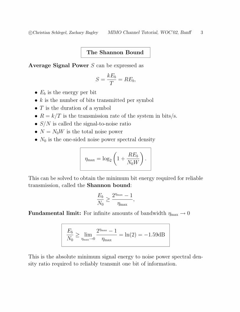
The Shannon Bound

Average Signal Power S can be expressed as

S =kEb

T= REb,

• Eb is the energy per bit

• k is the number of bits transmitted per symbol

• T is the duration of a symbol

• R = k/T is the transmission rate of the system in bits/s.

• S/N is called the signal-to-noise ratio

• N = N0W is the total noise power

• N0 is the one-sided noise power spectral density

ηmax = log2

(1 +

REb

N0W

).

This can be solved to obtain the minimum bit energy required for reliabletransmission, called the Shannon bound:

Eb

N0≥ 2ηmax − 1

ηmax,

Fundamental limit: For infinite amounts of bandwidth ηmax → 0

Eb

N0≥ lim

ηmax→0

2ηmax − 1

ηmax= ln(2) = −1.59dB

This is the absolute minimum signal energy to noise power spectral den-sity ratio required to reliably transmit one bit of information.


Normalized Capacity

Normalize our formulas per signal dimension as given by [WoJ65]. This isuseful when the question of waveforms and pulse shaping is not a centralissue, since it allows one to eliminate these considerations by treatingsignal dimensions [Schl97].

Cd =1

2log2

(1 + 2

RdEb

N0

)[bits/dimension]

Cc = log2

(1 +

REb

N0

)[bits/complex dimension]

Shannon bound normalized per dimension

Eb

N0≥ 22Cd − 1

2Cd;

Eb

N0≥ 2Cc − 1

Cc.

System Performance Measure In order to compare different commu-nications systems we need a parameter expressing the performance level.It is the information bit error probability Pb and typically falls into therange 10−3 ≥ Pb ≥ 10−6.

References:

[WoJ65] J.M. Wozencraft and I.M. Jacobs, Principles of Communication Engineering, JohnWiley & Sons, Inc., New York, 1965, reprinted by Waveland Press, 1993.

[Schl97] C. Schlegel, Trellis Coding, IEEE Press, Piscataway, NJ, 1997.


Spectral Efficiencies of Popular Systems

Spectral Efficiencies versus power efficiencies of various coded and un-coded digital transmission systems, plotted against the theoretical limitsimposed by the discrete constellations.

Unachieva

ble

Region

QPSK

BPSK

8PSK

16QAMBTCM32QAM

Turbo65536

TCM16QAM

ConvCodes

TCM8PSK

214 Seqn.

214 Seqn.

(256)

(256)

(64)

(64)

(16)

(16)

(4)

(4)

32QAM

16PSK

BTCM64QAM

BTCM16QAM

TTCM

BTCBPSK

(2,1,14) CC

(4,1,14) CCTurbo65536

Cc [bits/complex dimension]

-1.59 0 2 4 6 8 10 12 14 15

0.1

0.2

0.3

0.4

0.5

1

2

5

10

EbN0

[dB]

BPSK

QPSK

8PSK

16QAM

16PSK

ShannonBound


Discrete Capacities

For discrete constellations, Shannon’s formula needs to be altered.

C = maxq

[H(Y )−H(Y |X)] (classic definition)

= maxq

−∫y

∑ak

q(ak)p(y|ak)log

q(a′k)∑a′k

p(y|a′k)

−∫y

∑ak

q(ak)p(y|ak) log (p(y|ak))]

= maxq

[∑ak

q(ak)

∫y

log

(p(y|ak)∑

a′kq(a′k)p(y|a′k)

)]

where {ak} are the K discrete signal points, q(ak) is the probability withwhich ak is selected, and

p(y|ak) =1√

2πσ2exp

(−(y − ak)2

2σ2

)in the one-dimensional case, and

p(y|ak) =1

2πσ2 exp

(−(y − ak)2

2σ2

)in the complex case.

Symmetrical Capacity: When q(ak) = 1/K, then

C = log(K)− 1

K

∑ak

∫n

log

∑a′k

exp

(−(n− a′k + ak)

2 − n2

2σ2

)


Code Efficiency

Shannon et. al. [SGB67] proved the following lower bound on the codeworderror probability PB:

PB > 2−N(Esp(R)+o(N)); Esp(R) = maxq

maxρ>1

(E0(q, ρ)− ρR))

E0(ρ,q) ≡ − log2

∫y

(∑x

q(x)p(y|x)1/(1+ρ)

)1+ρ

dy

The bound is plotted for rate R = 1/2 for BPSK modulation [ScP99],together with selected Turbo and classic concatenated coding methods:

N=44816-state

N=36016-state

N=13344-state

N=133416-state

N=4484-state

N=204816-state

N=2040 concatenated (2,1,8) CCRS (255,223) code

N=2040 concatenated (2,1,6) CC +RS (255,223) code

N=1020016-state

N=1638416-state N=65536

16-state

N=4599 concatenated (2,1,8) CCRS (511,479) code

N=1024 block Turbo code using (32,26,4) BCH codes

UnachievableRegion

ShannonCapacity

10 100 1000 104 105 106

−1

0

1

2

3

4

EbN0

[dB]

N

References:[SGB67] C.E. Shannon, R.G. Gallager, and E.R. Berlekamp, “Lower bounds to error proba-

bilities for coding on discrete memoryless channels,” Inform. Contr., vol. 10, pt. I, pp.65–103, 1967, Also, Inform. Contr., vol. 10, pt. II, pp. 522-552, 1967.

[ScP99] C. Schlegel and L.C. Perez, “On error bounds and turbo codes,”, IEEE Communi-cations Letters, Vol. 3, No. 7, July 1999.


Parallel Additive Gaussian Channels

Let us assume that we haveN parallel one-dimensional channels disturbedby noise sources with variances σ2

1, · · · , σ2N .

+

+

x1

xN

y1

yN

N (0, σ21)

N (0, σ2N)

Energy Constraint: The total input energy is constrained on averageto E, the total average energy per channel use:

N∑n=1

x2n =

N∑n=1

En = E

The capacity of these parallel channels is achieved by

σ2n + En = µ; σ2

n < µ

En = 0; σ2n ≥ µ

where µ is the Lagrange multiplier chosen such that∑

nEn = E.

Theorem: The capacity of this set of parallel channels is given by

C =N∑n=1

1

2log

(1 +

En

σ2n

)=

N∑n=1

1

2log

(µ

σ2n

)

References:

[Gal68] R.G. Gallager, Information Theory and Reliable Communication, John Wiley & Sons,Inc., New-York, 1968, Section 7.5, pp. 343 ff.


Waterfilling Theorem

Proof: Let x = [x1, · · · , xN ] and y = [y1, · · · , yN ] and consider

I(x;y)(1)≤

N∑n=1

I(xn; yn) (1) independent xn

(2)≤

∑n=1

1

2log

(1 +

En

σ2n

)︸︷︷︸

f(E)

(2) Gaussian distributed xn

Since equality can be achieved the next step is to find the maxi-mizing energy distribution E = [E1, · · · , EN ].

∂f(E)

∂En≤ λ

1

2(σ2n + En)

≤ λ

σ2n + En ≤

1

2λ= µ

This theorem is called the Waterfilling Theorem. Its operation can bevisualized in the following figure, where the power levels are in black:

Power level:Difference µ− σ2n

µ

Channels 1 through N

level: σ2N


Correlated Parallel Channels (MIMO)

Correlated channels arise from e.g., multiple antenna channels:

+

+

+xNt

x1

x2

h11

hNtNr

hij

yNr

y2

y1

nNr

n2

n1

Transmit

Antenna

Array

Receive Array

This channel is a multiple-input multiple-output (MIMO) channeldescribed by the matrix equation:

y = Hx+ n

• The transmitted signals xn are complex signals, as are the channelgains hij and the received signals yn.

• The noise is complex additive Gaussian noise with variance N0 (thatis N0/2 in each dimension).

• The path gains hij are complex gain coefficients modeling a randomphase shift and a channel gain. Often these are modeled as Rayleighrandom variables modeling a scattering-rich or mobile radio trans-mission environment.

MIMO Rayleigh Channel: The hij are modeled as i.i.d. (or correlated)complex Gaussian random variables with variance 1/2 in each dimension.


Channel Decomposition

The correlated MIMO channel can be decomposed via the singular valuedecomposition SVD:

H = UDV +

(if r < t)

where U and V are unitary matrices, i.e., UU+ = I, and V V + = I.The matrix D contains the singular values of H , which are the (positive)square roots of the eigenvalues of HH+ and H+H .

The channel equation can now be written in an equivalent form:

y = Hx+ n

= UDV +x+ n

U+y = y = Dx+ n

If Nt > Nr only the first Nr signals ofx will be received.If Nr > Nt the Nr − Nt “bottom”channels will carry no signal.

This leads to parallel Gaussian channels yn = dnxn + nn

+

+

+

+

x1

xN

y1

yN

N (0, 2σ2)

N (0, 2σ2)

d1

dN N = min(Nt, Nr)


MIMO Capacity

The multiplicative factors dn can be eliminated by multiplying the re-ceived signal y with D−1. This leads back exactly to the parallel chan-nels:

C =N∑n=1

log

(1 +

d2nEn

2σ2

)=

N∑n=1

log

(d2nµ

2σ2

)

Note: The channels are complex, and hence there is no factor 1/2 and thevariance is 2σ2.

This capacity is achieved with the waterfilling power allocation:

2σ2

d2n

+ En = µ;σ2

d2n

< µ

En = 0;σ2

d2n

≥ µ

Optimal System: This leads to the optimal signalling strategy:

1. Perform the SVD of the channel H → U ,V ,D.

2. Multiply the input signal vector x with V . This is matrix processing.

3. Multiply the output signal y with the matrix processor U+.

4. Use each channel with signal-to-noise ratio d2nEn/(2σ

2) independently.

x x y yV U+

Matrix Processor Matrix ProcessorMIMO Channel


Symmetric MIMO Capacity

Drawback: the channel H needs to be known at both the transmitterand the receiver so the SVD can be computed.

Fact: Channel knowledge is not typically available at the transmitter,and the only choice we have is to distribute the energy uniformly over allcomponent channels. This leads to the Symmetric Capacity:

C =N∑n=1

log

(1 +

d2nE

2Ntσ2

)= log

N∏n=1

(1 +

d2nE

2Ntσ2

)

Noting that the d2n are the eigenvalues ofHH+, the above formula can be

written in terms of matrix eigenvalues, using the fact det(M) =∏λ(M),

and det(I +M) =∏

(1 + λ(M )):

C = logN∏n=1

(1 +

d2nE

2Ntσ2

)= log det

(INr +

E

2Ntσ2HH+)

= log det

(INr +

E

2Ntσ2H+H

)

Discussion:

• The capacity of a MIMO channel is goverend by the singular valuesof H , or in the symmetrical case by its eigenvalues. These determinethe channel gains of the independent parallel channels.

• ChannelH needs to be known at the receiver→ Channel Estimation

• This implies a study of the behavior of channel eigenvalues.


MIMO Fading Channels

Assumed that the channel H is known at the receiver

I(x; (y,H)) = I(x;H) + I(x;y|H)

= I(x;y|H)

= EH [I(x;y|H = H0)]

We need to average the mutual information over all channel realizations.

I(x;y|H) is maximized if x iscircularly symmetric complex Gaussian with covariance Q, and

I(x; (y,H)) = EH

[log det

(Ir +

E

2Ntσ2HQH+)]

I(x; (y,H)) = EH

[log det

(Ir +

E

2Ntσ2 (HU )D(U+H+)

)]• The spectral decomposition of Q = UDU+ produces an equivalent

channel H = HU , hence the maximizing Q is diagonal.

• Furthermore, concavity of the function log det() shows that Q = I,hence the maximizing Q is a multiple of the identity

Capacity of the MIMO Rayleigh Channel:

C = EH

[log det

(INr +

E

2Ntσ2HH+)]

• By the law of large numbers:

HH+ Nt→∞−→ NtIr and C = Nr log

(1 +

E

2σ2

)H+H

Nr→∞−→ NrI t and C = Nt log

(1 +

Nr

Nt

E

2σ2

)


Evaluation of the Capacity Formula

Following Telatar [Tel99] define the random matrix

W =

{HH+ if Nr < Nt

H+H if Nr ≥ Nt

W is an m×m;m = min(r, t) non-negative definite matrix with real,non-negative eigenvalues µn = d2

n

The capacity can be written in terms of these eigenvalues:

C = E{µn}

[N∑n=1

log

(1 +

E

2Ntσ2µn

)] for r = t symmetric chan-nels, let {λn} be the eigen-values of H , then µn = λ2

n

• The (ordered) eigenvalues of W follow a Wishart distribution:

p(µ1, · · · , µN) = α

N∏i=1

e−µiµM−Ni

∏i<j

(µi − µj)2

︸︷︷︸det

1 ··· 1µ1 ··· µN...

...µN−1

1 ··· µN−1N

;M = max(Nr, Nt)

• C depends only on the distribution of a single unordered eigenvalue:

C = NE{µ}

[log

(1 +

µE

2Ntσ2

)]=

∫ ∞0

Np(µ) log

(1 +

µE

2Ntσ2

)dµ

This integration evaluates to

C =

∫ ∞0

log

(1 +

µE

2Ntσ2

)N−1∑k=1

k!

(k +M −N)![LM−Nk (µ)]2µM−Ne−µdµ

• LM−Nk (x) = 1k!e

x dk

dxk(e−xxM−N+k) is the Laguerre polynomial of order k


Large Systems

As the number of antennas Nt →∞, Nr →∞, the number of eigenvaluesN(µ)→∞, and the capacity formula

C = E{µi}

[N∑i=1

log

(1 +

µE

2Ntσ2

)]→∫ ∞

0N log

(1 +

µNE

2Ntσ2

)dFµ(µ)

Fµ(µ) is the cumulative distribution (CDF) of the eigenvalues of W

For random matrices like W , a general result states

dFµ(µ)

dµ→

1

2π

√(µ+

µ − 1)(

1− µ−µ

); forµ ∈ [µ−, µ+]

0 otherwise

2 4 6 8

0.1

0. 2

0. 3

0. 4

0. 5

• MN → τ ≥ 1, and µ± = (

√τ ± 1)2.

τ = 1

τ = 2

τ = 4

In the limit, the capacity of the Rayleigh MIMO is given by

C

N=

1

2π

∫ d+

d−

log

(1 +

µNE

2Ntσ2

)√(µ+

µ− 1

)(1− µ−

µ

)dµ

Reference:

[Tel99] I.E. Telatar, “Capacity of mulit-antenna Gaussian channels”, Eur. Trans. Telecom.,Vol. 10, pp. 585–595, Nov. 1999.


Physical Channel Modeling

Objective: Model realistic correlation among the statistical parametersof the channel parameters based upon ray-tracing models.

Method: Emulate the correlated complex path gains represented by theelements of the channel matrix H using basic ray tracing techniques with:

• Symbol time Ts set large enough such that flat fading occurs.

• Randomly placed scattering objects inside a ring of radius R meters.

• Elements spaced d carrier wavelengths apart.

• Transmitter and receiver arrays separated by L meters.

L

R

The sampled path gain between the ith receiver element and the jth trans-mitter element at time nTs is the complex superposition:

hij(n) = A

K∑k=1

gke−j(θk+2πfdknTs)

The random variables gk, θk, and fdk determine hij(n) as the superpositionof K electromagnetic waves as follows:

• gk is the amplitude of the kth wave at time nTs• θk is the kth phase term

• fdk is the Doppler error frequency determined by angle of arrival

• hij(n) is normalized to unit power


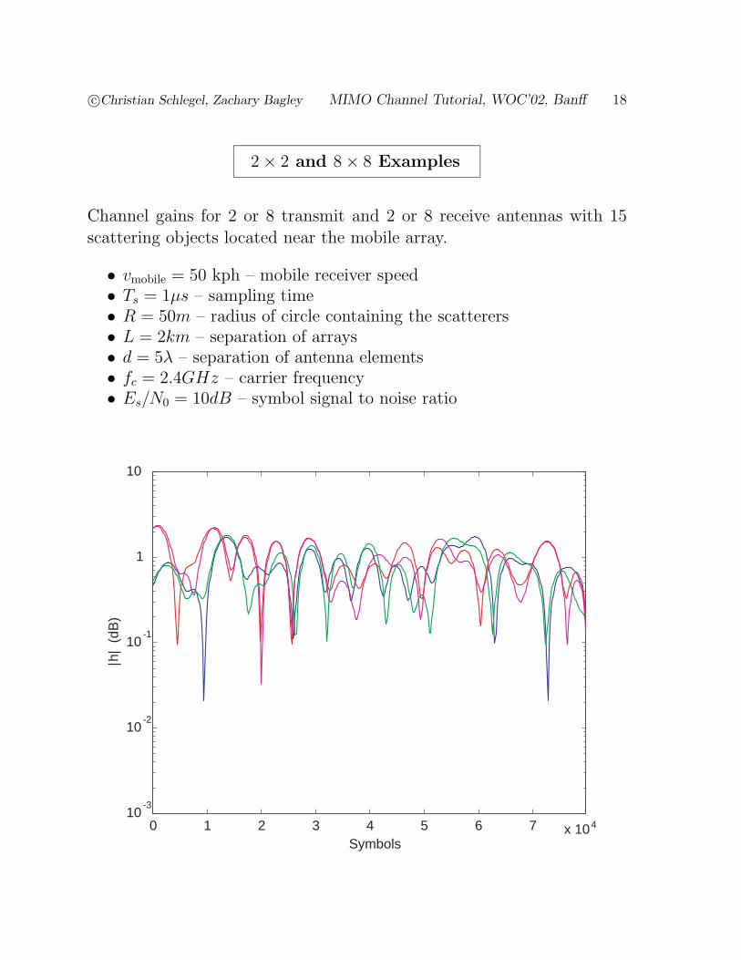
2× 2 and 8× 8 Examples

Channel gains for 2 or 8 transmit and 2 or 8 receive antennas with 15scattering objects located near the mobile array.

• vmobile = 50 kph – mobile receiver speed• Ts = 1µs – sampling time• R = 50m – radius of circle containing the scatterers• L = 2km – separation of arrays• d = 5λ – separation of antenna elements• fc = 2.4GHz – carrier frequency• Es/N0 = 10dB – symbol signal to noise ratio

0 1 2 3 4 5 6 7 x 10410

-3

10-2

10-1

1

10

Symbols

| h |

(dB

)


Capacities for the 2× 2 and 8× 8 Channels

Capacities of correlated and uncorrelated channels:

• 8× 8 and 2× 2 antenna arrays ideally uncorrleated (red lines)

• 8× 8 and 2× 2 antenna arrays corrleated by the scattering process(blue lines)

Note: The relative variance decreases with the number of antennas.

0 1 2 3 4 5 6 7 8 9 10 x10 40

5

10

15

20

25

30

35

Symbols

Cap

acity

(bi

ts/c

hann

el u

se)

Reference:

[Scb02] C. Schlegel and Z. Bagley, “Efficient processing for high-capacity MIMO channels,”submitted to IEEE J. Select. Areas Commun., Special Issue: MIMO Systems, May 2002.

[BaS01] Z. Bagley and C. Schlegel, “Classification of correlated flat fading MIMO channels(multiple antenna channels),” CIT 2001, June 3-6, Vancouver, BC.


Characteristics of the MIMO Channel

Rank ClassificationMIMO channels can be classified as high-rank or low-rank channels.

This classification is made based upon correlation properties of the re-ceiver array response vector, or the singular values of the channel responsematrix H .

Orthogonal channel path gains present the upper limiting case for theMIMO channel capacity. In this case, the non-zero squared singular val-ues of the channel response matrix H are given by

d2n = NrE{h+

nnhnn}, i = 1, 2, · · · , Nt

Statistically indepedent channel path gains hij are usually modelledas uncorrelated complex Gaussian random variables. In this case, theeigenvalues of HH+ for Nt ≥ Nr and H+H for Nt ≤ Nr are given bythe previously described Wishart distribution.

Correlated channel path gains occur in real-world cases. The completelycorrelated case such as in long-distance scatter-free wireless links identifiesthe lower capacity limit for MIMO channels. In this case, the single non-zero squared singular value of the channel response matrix H is

d2 = Nr

Nt∑n=1

E{h+nnhnn} = NrNt,

References: (for linear algebraic concepts)

[HrJc99] R.A. Horn and C.R. Johnson, “Matrix Analysis”, Cambridge University Press 1999.


High-Rank MIMO Channels

High-rank MIMO channels occur when there is a rich scattering envi-ronment and when the Tx and Rx arrays are relatively near one another.

• High rank MIMO channels occur when there is little correlationamong the channel path gains.

• MIMO channels have a diversity gain defined by the rank of HH+.

• The maximum achievable diversity gain is

rank(HH+) = min(Nt, Nr)

• The orthogonal channel gain case represents the upper limit for thecapacity of MIMO channels, and the maximum diversity gain.

If theNt columns ofH are orthogonal and the entries ofH are normalizedto unit power, the squared non-zero singular values of H are:

d2n = Nr; n = 1, 2, · · · , Nt

Capacity:The capacity of the high-rank MIMO channel can now be written as

Chigh =

min(Nr,Nt)∑i=1

log

(1 +

ρd2n

Nt

); ρ =

E

2σ2

≈ min(Nt, Nr)︸︷︷︸array capacity

advantage

log

(1 +

ρNr

Nt

)︸︷︷︸

receiver antennaSNR advantage


Low-Rank MIMO Channels

Low rank MIMO channels occur under scatter-free or long-distancelinks. The low rank MIMO channel is equivalent to a single antennachannel with the same total power.

• Low rank MIMO channels occur when there is strong correlationbetween the channel path gains.

• The correlation characteristics determine the rank of HH+, whichin turn determines the diversity advantage.

• A completely correlated H matrix is a scaled version of the all one’smatrix with with dimensions Nr×Nt and provides no diversity gainover the single antenna case.

If the paths are highly correlated, all gains hij are roughly equal, and H ,a multiple of the all-one matrix, has a single non-zero singular value

d2 = Nr

Nt∑n=1

E{h+nnhnn} ≈ NrNt,

Capacity:The capacity of the low-rank MIMO channel can now be written as

Clow =

min(Nr,Nt)∑n=1

log

(1 +

ρ

Ntd2n

)≈ log

(1 +

ρ

Ntd2)

≈ log (1 + ρNr) .

Note: The channel behaves like a point-to-point channel with Nr timesthe received signal power due to the antenna array, achieved bysimple maximum-ratio combining at the receiver


Low-SNR MIMO Channels

If the available ρ is low, a Taylor Series approximation of

log(1 + x) ≈ x

for small values of x lets us develop both Chigh and Clow as

Chigh ≈ min(Nr, Nt)ρNr

Nt; Clow ≈ ρNr.

Furthermore, these formulas present overbounds to the actual capacities

Conclusions:

• Correlation in the channel has little effect on capacity for low SNR.

• Correlation in the channel has a pronounced effect where the linearapproximation to log(1 + x) does not apply.

• The MIMO resources must be allocated differently based upon theclassification of the MIMO channel.

• Easily estimated correlation statistics can be used to help classifythe operating conditions as high-rank or low-rank.


High and Low-Rank MIMO Channel Capacities

The following figures the general capacity behavior for high and low rankMIMO channels ρ values of 0 dB and 20 dB.

Bits/channel use

Bits

ρ

ρ2 4 6 8 10 12 14 16 18 200

0.5

1

1.5

2

2.5

3

High correlation (case H)Low correlation (case L)

Capacity as a function ofthe number of antennas inthe arrays

2 4 6 8 10 12 14 16 18 200

20

40

60

80

100

120

High correlation (case H)Uncorrelated Fading

Low correlation (case L)

Standard deviation of thecapacity as a function ofthe number of antennas

References:

[Tel99] I.E. Telatar, “Capacity of mulit-antenna Gaussian channels”, Eur. Trans. Telecom.,Vol. 10, pp. 585–595, Nov. 1999.

[BaS01] Z. Bagley and C. Schlegel, “Classification of correlated flat fading MIMO channels(multiple antenna channels),” Canadian Information Theory Workshop, CITW’2001,Vancouver, BC, June 3–6, 2001.


Effects of the Array Geometry

The condition for orthogonality between the columns ofH in a scatterfreeenvironment is given by [GBGP01]

dtdrL

=λ

Nr.

• dt and dr are the Tx and Rx antenna array element seperations

• L is the distance between arrays

• Nr is the number of receiver elements

• λ is the carrier wavelength

The following figure illustrates the transition from a high rank channelto a low rank channel for high and low SNR values and for two valuesof the element separation.

100

101

102

103

104

105

0

5

10

15

20

25

L / r

Cap

acity

(bi

ts /

use)

Capacity versus Link Seperation to Scattering Radius Ratio for Nt = N

r = 4

SNR = 20 dB

SNR = 0 dB

d = 5 wavelengths (BLUE)

d = 1 wavelength (RED)


Capacity Advantage Factor

From the previous figure, it is easy to conclude that scatter-free linksdegrade to equivalent single-antenna channels very quickly, leading tothe “pin-hole channel” described by the correlated channel capacity

Clow ≈ log (ρNr) (1)

Under high SNR conditions, the capacity formula can be approximatedas

C =N∑n=1

log

(1 +

ρ

Ntd2n

)

≈N∑n=1

log

(ρ

Ntd2n

)= log

(N∏i=1

ρ

Ntd2n

). (2)

• N = rank(HH+)

• The total instantaneous capacity is a function of the rank of HH+,or equivalently the condition number of HH+.

• Link geometry determines correlation and fading parameters.

• The H matrix entries become highly correlated rather quickly rela-tive to the antenna element separation parameters [GBGP01].

Comparing (1) and (2), we can define a capacity benefit factor repre-senting the capacity gain (at high SNR values) over the pin-hole channelsince

log

(N∏n=1

ρ

Ntd2n

)≥ log (ρNr)

which after collecting terms becomes

log

[(ρ

Nt

)N−1 ∏Nn=1 d

2n

NtNr

]≥ 0


Capacity Advantage Factor

Noting that

C − Clow ≈ log

[(ρ

Nt

)N−1 ∏Nn=1 d

2n

NtNr

]= log(α) ≥ 0,

we can write the capacity under high SNR conditions in terms of thecapacity advantage over the “pin-hole” channel:

C ≈ logα + Clow = log(α ρNr), α =

(ρ

Nt

)N−1 ∏Nn=1 d

2n

NtNr

10 5 0 5 10 15 20 250

10

20

30

40

50

60

70

ρ / N0 (dB)

Cap

acity

(bi

ts/u

se)

Csym, Cwaterfilling (orthogonal)

Csym, Cwaterfilling (i.i.d)

Clow + log(α)

Chigh

Clow

References:[GBGP01] D. Gesbert, H. Bolcskei, D. A. Gore, A. J. Paulraj, “Outdoor MIMO Wireless Chan-

nels: Models and Performance Prediction,” submitted to IEEE Trans. Communications,July 2000.

[ScB02] C. Schlegel and Z. Bagley, “Efficient Processing for High-Capacity MIMO Channels,”submitted to IEEE J. Select. Areas Commun., Special Issue: MIMO Systems, May 2002.

[Bag02] Z. Bagley, “Serially Concantenated and Layered Space-Time Coding,” Ph.D. thesis,work in progress.

SPACE-TIME MODULATION


Space-Time Coding

Space-time coding (STC) systems make use of the MIMO channel gener-ated by a multiple-antenna transmit/receive setup:

+

+

+xNtr

x1r

x2r

h11

hNtNr

hij

yNrr

y2r

y1r

nNrr

n2r

n1r

Transmit

Antenna

Array

Receive Array

Each antenna transmits a DSB-SC signal:

yj(t) =

Nt∑i=1

√Es

Nthijxi(t) + ni(t)

and y(t) =

√Es

NtHx(t) + n(t),

where y = (y1, · · · , yNr) and x = (x1, · · · , xNt).

Channel Gains: modeled as independent complex coefficients, i.e.,

p(h) =1

2πexp

(−|h|

2

2

); E[hihj] = 0

which leads to a Rayleigh distributed amplitude

p(a = |h|) = a exp

(−a

2

2

)p(a = |h|2) =

1√2πa

exp(−a/2)


MIMO Channels → Transmit Diversity

The Alamouti scheme [Ala98] uses two transmit antennas:

+

[x1, x∗0]

[x0,−x∗1]

h1

h0

[x0,−x∗1][x0, x1]

[h0, h1]

Transmit

Antenna

Array

Combiner

Estimate

The transmitted 2 × 2 STC codeword is X, and thesymbols xi can be any quadrature modulated symbols.

X =

[x0 −x∗1x1 x∗0

]

The received signal for a single receive antenna is

r = [r0, r1] = [h0x0 + h1x1,−h0x∗1 + h1x

∗0] + [n0, n1]

= [h0, h1]X + n

The demodulator calculates

[x0, x1] =

[h∗0 −h1

h∗1 h0

] [r0

−r∗1

]

=

(|h0|2 + |h1|2)x0 + h∗0n0 + h1n∗1︸︷︷︸

n′0

, (|h0|2 + |h1|2)x1 + h0n∗1 + h∗1n0︸︷︷︸n′1

• If the channel path h0 and h1 are uncorrelated, the noise sources n′i

have twice the variance of the original noise sources.

• The system provides dual diversity due to the factor (|h0|2 + |h1|2)which exhibits a χ-square distribution of fourth order.

Reference:

[Ala98] S.M. Alamouti, “A simple transmit diversity technique for wireless communications,”IEEE J. Select. Areas Commun., Vol. 16, No. 8, October 1998.


Multiple Receive Antennas

The Alamouti scheme can be extended to multiple receive antennas:

R =

[r0 r1

r2 r3

]=

[h0 h1

h2 h3

] [x0 −x∗1x1 x∗0

]+N

Multiplying the received signalsR with the channel estimateH we obtain

[x0, x1] =

[h∗0 −h1

h∗1 h0

] [r0

−r∗1

]+

[h∗2 −h3

h∗3 h2

] [r2

−r∗3

]= (|h0|2 + |h1|2 + |h2|2 + |h3|2)x0 + h∗0n0 + h1n

∗1 + h∗2n2 + h3n

∗3︸︷︷︸

n′0

,

+ (|h0|2 + |h1|2 + |h2|2 + |h3|2)x1 + h0n∗1 + h∗1n0 + h∗2n2 + h3n

∗3︸︷︷︸

n′1

]

This system provides 4-fold diversity as expressed by the amplitude

A = (|h0|2 + |h1|2 + |h2|2 + |h3|2)

This is possible due to the fact that the rows of X are orthogonal. TheAlamouti scheme is the most basic representative of what are known as

Orthogonal DesignsReal: The following is an example of a 4× 4 (real) orthogonal design

X =

x1 x2 x3 x4

−x2 x1 −x4 x3

−x3 x4 x1 −x2

−x4 −x3 x2 x1

Complex: A rate R = 0.5 complex design is

X =

x1 −x2 −x3 −x4 x∗1 −x∗2 −x∗3 −x∗4x2 x1 x4 −x3 x∗2 x∗1 x∗4 −x∗3x3 −x4 x1 x2 x∗3 −x∗4 x∗1 x∗2


Space-Time Orthogonal Block Codes (STOB)

STOBs are based on the theory of orthogonal designs [TJC99].As 3× 4 real orthogonal design is

X = D4,3(x) =

x1 x2 x3

−x2 x1 −x4

−x3 x4 x1

−x4 −x3 x2

XTX = KsI; Kx =L∑i=1

x2i

This STOB is used to drive 3 transmit antennas:

[x1,−x2,−x3,−x4]

[x2, x1, x4,−x3]

[x3,−x4, x1, x2]h3

h2

h1

h = [h1, h2, h3]T

GTrx3

x2

x1

x4

The received signal at (each) receive antenna is

r = Xh+ n =

h1 h2 h3 0h2 −h1 0 −h3

h3 0 −h1 h2

0 h3 −h2 −h1

x1

x2

x3

x4

+ n = Gx+ n

G = D4,4([h1, h2, h3, h4 = 0]) is also an orthogonal design: GTG = KhI.Optimal reception is ackomplished with a matched filter receiver

x =1

Kh= GTr = x+ n; Kh =

Nt∑i=1

|hi|2

Reference:

[TJC99] V. Tarokh, H. Jafarkhani, and A.R. Calderbank, “Space-time block codes from or-thogonal designs,” IEEE Trans. Inform. Theory, vol. 45, no. 5, July 1999.


STOB: Diversity and SNR Gains

Processing at each receive antenna is identical, and the Nr channels foreach symbol xj are added together (Maximum-ratio combining):

+

+

+

BasebandSignals

r1

rNr

gTNr,1

gT11

gT12

gT1,Nc

x1

x2

xNc

DespreadingMR Combining

Diversity and SNR

• It is straightforward to see that xj =√a2jxj + nj, where a2

j is χ2-

distributed with degree NtNr, and 2NtNr for complex designs.

• The noise nj has power NrN0/2, and NrN0 for complex designs.

Diversity Gain : γd =NtNr

2

SNR Gain : ρd =

∑NtNri=1 |hi|2NtN0/2

• Complex orthogonal designs exist only for rates R ≤ 1/2, i.e., thereare at most L/2 orthogonal vectors.

• On the other hand, real orthogonal designs do exist for R ≤ 1, i.e.,there exist up to L real orthogonal vectors.

• Orthogonal designs can be used with single-sideband modulation


STOB: Capacity and Spectral Efficiency

• Space-time orthogonal codes completely separate the L ≤ Nt (L ≤Nt/2 in the case of complex signals) channels and have a very simpleoptimal receiver structure.

• Each of the separated channels has a χ2 distributed power level withdegree NtNr, which is close to constant.

• Nevertheless the restriction to STOBs causes a loss in capacity

Capacity of STOB

Transmit Power: Pt = NcEs/Nt; (Nc symbols transmitted).

Received Power/Antenna: Pr = (NtNr)2Es/Nt, each path contributes.

Noise Power/Antenna: Pn = NtNrN0/2, each receive antennacontributes a noise source.

STOB Capacity is then given by the applying Shannon’s formula:

CSTOB =Nc

Llog

(1 +

2NrEs

N0

); (bits/channel use)

Notes:

• CSTOB is directly proportional to the rate R = NcL of the orthogonal

design

• The SNR gain is proportional to the number of receive antennas –nothing else

• The large diversity ensures that the amplitude fluctuations are min-imal → Capacity identical to that of an AWGN.


STOB Capacity: Example

Capacities of 8 × 8 Systems: Comparison between the MIMO sym-metric capacity and the STOB capacity for an 8×8 multiantenna system.

MIMO LimitSTOB CapacityAWGN Capacity

-10 -5 0 5 10 15 200.1

1

10

102Bits/Channel Use

40 bits

9dB

one sideband

both sidebands

Es/N0

Observation: STOB codes provide adiversity advantage but do not provideany capacity advantage over a point-to-point channel with the same resources.


Space-Time Codes: Error Computation

In general a space-time codeword is an Nt×Nr matrix (array) of complexsignals:

X = [x1, · · · ,xNc] =

x11 x12 · · · x1Nc...

...xNt1 xNt2 · · · xNtNc

Each row of X is a space-time symbol, and the received STC word is

Y =

√Es

NtHX +N

This means the conditional probability density function of Y given Hand the transmitted STC codeword is multi-variant Gaussian:

p(Y |H ,X) =1

πNrNcexp

−tr

{(Y −

√EsNtHX

)(Y −

√EsNtHX

)+}

2N0

Note: The exponent term tr

{MM+} is merely the squared sum of all

the entries in M .

• N is a matrix of complex noise samples with variance N0, that isvariance σ2 = N0/2 in each of the two dimensions.

• The signal energy per space-time symbol is√Es and

√EsNt

per con-

stellation point• Each constellation point xij is energy normalized to unity.


Space-Time Codes II: Optimal Decoding

ML reception: The ML-receiver requires channel knowledge and andmaximises the squared metric

X = arg minX

[tr

{(Y −

√Es

NtHX

)(Y −

√Es

NtHX

)+}]

= arg minX

[tr

{Es

NtHXX+H+

}− 2tr

{√Es

NtHXY +

}]

Fixed Channels

At any given time-instant, the channel is fixed and the impairment isGaussian noise.Pairwise Error Probability

P (X →X ′) = Q

√Es

Nt

d2(X,X ′)

2N0

Squared Euclidean Distance

d2(X,X ′) =Es

Nt

Nc∑n=1

Nr∑j=1

∣∣∣∣∣Nt∑i=1

hij(xin − x′in)∣∣∣∣∣2


Squared Euclidean Distance (SED)

d2(X,X ′) can be expressed in terms of H ,X and X ′ as

d2(X,X ′) =Es

Nt

Nr∑j=1

Nt∑i=1

Nt∑i′=1

hijh∗i′j

Nc∑n=1

(xin − x′in)(xi′n − x′i′n)∗︸︷︷︸Kii′

The matrix K is a kernel matrix with entries Kii′.

SED as a Quadratic FormDefine hj = [h1j, · · · , hNtj]T as the signature vector of receive antenna j.

d2(X,X ′) =Es

Nt

Nr∑j=1

h∗jKhj

Since K is hermitian (K = K+), we can spectrally decompose d2(X,X ′)

d2(X,X ′) =Es

Nt

Nr∑j=1

h∗jV DV+hj

=Es

Nt

Nr∑j=1

v∗jDvj

The components of these equations are:

• V is a unitary matrix

• D is a diagonal matrix with the eigenvalues of K. It can be shownthat all these eigenvalues are nonnegative real

• h is a vector of complex Gaussian gains

• v = V +h is a vector of rotated complex channel gains


STC Error Probability

The SED can be expressed in terms of the eigenvalues of K

d2(X,X ′) =Es

Nt

Nr∑j=1

Nt∑i=1

di|vij|2; vj = V +hj

and, given a fixed channel H

P (X →X ′) = Q

√Es

∑Nrj=1∑Nt

i=1 di|vij|22N0Nt

Error Probability depends on the eigenvalues of the matrix

K = (X −X ′) (X −X ′)+

in particular on the rank and the product of the eigenvalues.

Chernoff Bound is easier to manipulate:

P (X →X ′) ≤ exp

(− Es

4N0Nt

Nr∑j=1

Nt∑i=1

di|vij|2)

=

Nr∏j=1

exp

− Es

4N0Nt

Nt∑i=1

di|vij|2︸︷︷︸Dj


Fading Error Analysis

Fading channels: If independent fading is assumed then

• h is a vector of independent complex Gaussian random variables

• v = V +h is also a vector of independent complex Gaussian randomvariables, because

E[vv+] = V +E

[hh+]V = I

The components vij are unit-variance complex Gaussian random vari-ables, |vij|2 is χ-square distributed with two degrees of freedom:

p(a = |v|2) = exp(−a); p(da = d|v|2) =1

dexp(−a/d)

d2(X,X ′) is the weighted sum of χ-square random variables.

PDF of SED The PDF is found via a partial fraction expansion of thecharacteristic function:

p(x = d2) =

Nt∑i=1

pi

Nr∑j=1

xm−1

dmi (m− 1)exp

(− xdi

)This PDF can be integrated in closed form to

Pe =1

2

Nt∑i=1

pi

Nr∑j=1

1− 1√1 + 4N0Nt

Esdi

m−1∑n=0

2n

22nn2

1(1+Esdi4N0Nt

)n

References:

[TNSC98] V. Tarokh, A.F. Naguib, N. Seshadri, and A.R. Calderbank, “Space-time codes forhigh data rate wireless communications: Performance criterion and code construction,”IEEE Trans. Inform. Theory, pp. 744–765, March 1998.

[BaS02] Z. Bagley and C. Schlegel, “Pair-wise error probability for space-time codes undercoherent and differentially coherent decoding,” submitted to IEEE Trans. Commun.,January 2002.

[Sch96] C. Schlegel, “Error probability calculation for multibeam Rayleigh channels,” IEEETrans. Commun., Vol. 44, No. 3, March 1996.


Chernoff Error Bounds

The Chernoff error bounding technique avoids many algebraic technical-ities. The bound is calculated from the characteristic function as:

P (X →X ′) ≤ E

[exp

(− Es

4N0Nt

Nr∑j=1

Nt∑i=1

di|vij|2)]

=

Nr∏j=1

Nt∏i=1

1

1 + Esdi4N0Nt

The final form of the bound is:

P (X →X ′) ≤(

1∏Nti=1(1 + Esdi

4N0Nt)

)Nr

≤(

Nt∏i=1

di

)−Nr(Es

4N0Nt

)NrNt

Design Criteria:

• The Rank Criterion: To achieve maximum diversity gain the ker-nel matrix K = (X −X ′)(X −X ′)+ has to have full rank.

• The Determinant Criterion: The product∏Nt

i=1 di = det(K)needs to be maximized to give maximum coding gain.

Orthogonal Designs revisited: Orthogonal designs provide full diver-sity. This condition is equivalent to requiring thatX−X ′ is non -singularfor any X 6= X ′.

Proof: The determinant of X is

det(X) =

√det(XXT ) =

√√√√det diag

(∑i

x2i , · · · ,

∑i

x2i

)=

[∑i

x2i

]Nt/2

and therefore

det(X −X ′) =

[∑i

|xi − x′i|2]Nt/2

6= 0

Therefore the maximum diversity NtNr is achieved.


Code Construction

Following these criteria Tarokh et. al. [TNSC98] have constructed trelliscodes which provide maximal diversity. For example:

00 01 02 03

10 11 12 13

20 21 22 23

30 31 32 33

22 23 20 21

32 33 30 31

02 03 00 01

12 13 10 11m(1),m(2) m(3),m(4) m(5),m(6) m(7),m(8)

These codes achieve full diversity on two-antenna systems. The transmis-sion rate is 2 bits per symbol using two QPSK signals over two antennas,because there are four choices at each state.

Decoding:Decoding follows the trellis using a sequence metric calculator→Viterbi.Branch Metrics:The Viterbi algorithm works by using metrics m(r) along their branchesand accumulates them to find the global minimum, where

m(r) =

Nr∑j=1

∣∣∣∣∣yjr −Nt∑i=1

hijxir

∣∣∣∣∣2

=⇒ need channel estimates

m(r) = ‖yr −Hxr‖2

The metric is simply the squared Euclidean distance between hypothesisand received signal.


Error Performance of STCs

4 states

8 states

16 states32 states

64 states

4 5 6 7 8 9 10 11 12 13 1410−4

10−3

10−2

10−1

1

Frame Error Probability (BER)

SNR


No Channel Information and Noncoherent Detection

If the channel H is not known at the receiver – the worst case – then Yconditioned only on X is Gaussian distributed since both N and H(t)are Gaussian distributed.If we decompose the channel equation

Y =

√Es

NtHX +N =

yT1...yTNr

=

√Es

Nt

hT1X + nT1...

hTNrX + nTNr

into signal sequences of different antennas, and consider the cross-correlationof the j-th sequence:

E[yjy

+j

]= E

[(X+hj + nj)(h

+j X + nj)

]= X+E

[hjh

+j

]X +N0I

If each receive antenna statistically sees the same channel, then this cross-correlation is independent of j and thus, for independent subchannels:

E[yjy

+j

]=Es

NtX+X +N0I = ΣX

In this case the conditional PDF of the received space-time codeword canbe written as:

p(Y |X) =exp

(−tr

{Y ΣX

−1Y +})πNrdetΣX


Noncoherent Detection and Unitary Space-Time Codes

Since the trace operator is invariant to a rotation of its arguments:

tr

{Y

(Es

NtX+X +N0I

)−1

Y +

}= tr

{(Es

NtX+X +N0I

)−1

Y +Y

}the following conclusions can be drawn:

(1) The Nc×Nc matrix Y +Y is a sufficient statisticfor optimal detection.

(2) p(Y |X) depends on X only through X+X.

(3) Unitarily rotated signals UX have the samePDF p(Y |X) = p(Y |UX).

Unitary Space-Time Codes: The transmitted signals over each an-tenna (rows of X) are orthogonal:

XX+ = NtI; detΣX = det

(Es

NtXX+ +N0I

)= Es +N0

Note: Unitary STC codewords X are not necessarily unitary matrices.For a matrix to be unitary it must be square and UU+ =U+U=I.

Using (A+BCD)−1 = A−1 − A−1B(C−1 +DA−1B)−1DA−1

Σ−1X = I − Es

NtEs + 1X+X

Optimal Detection: X = arg maxX

[tr{Y X+XY +}]


Unitary Space-Time Codes: Basic Properties

The non-coherent receiver and unitary STCs have the following properties

• the receiver is quadratic and requires no channel estimates.

• Unitary STCs send orthogonal signals over theNt transmit antennas.

• Orthogonal designs are unitary, but not necessarily visa versa.

• Orthogonal designs can be decoded non-coherently (without channelstate information)

• Using orthogonal spreading sequences for each antenna is one wayof achieving unitary STCs.

Capacity Result: It is shown in [MaH99] that for the block-wise con-stant channel unitary signals can achieve the capacity for non-coherentdetection.

Block-wise constant channels are a model for, e.g., frequency hoppingsystems, or interleaved fast fading channels.

Further results are:

• There is no point in using more transmit antennas than the coherenceduration of the channel, i.e., Nt ≤ Nc. The capacity is unchangedfor Nt ≥ Nc.

Reference:

[MaH99] T.L. Marzetta and B.M. Hochwald, “Capacity of a mobile multiple-antenna com-munication link in Rayleigh flat fading,” IEEE Trans. Inform. Theory., Vol. 45, No. 1,January 1999.


Unitary Group Codes

Hughes [Hug00] proposed the use of unitary group codes G, whose mem-bers G are unitary matrices. The transmitted codewords are:

X = TG

where T is a Nt×Nc transmission matrix adapting G to the transmissionsystem with Nt antennas.

Quaternion CodeA basic such unitary STC with Nc = 2, with elements in the quaternaryphase shift keyed (QPSK) constellation is

Q =

{±(

1 00 1

),±(j 00 −j

),±(

0 1−1 0

),±(

0 j

j 0

)}

This code can be used on a Nt = 2 antenna system with T =

(1 −11 1

)The group code Q is isomorphic to Hamilton’s quaternion group.

Differential Encoding of STCsThese codes are transmitted differentially as shown below:

+G(t) X(t)

X(t−1)

X(t) = X(t− 1)G(t); X(0) = T

Reference:

[Hugh00] B.L. Hughes, “Differential space-time modulation,” IEEE Trans. Inform. Theory,Vol. 46, No. 7, pp. 2567–2578, Nov. 2000.


Differential Reception

Unitary space-time codes can be differentially detected. This also requiresno channel state information, which is gleaned from a previously receivedSTC symbol.Considering a composite STC word consisting of two unitary STC words:

X2(t) = [X(t− 1) : X(t− 1)G]

we see that is fullfills the unitary condition for non-coherent detection:

X2(t)X2(t)+ = [X(t− 1) : X(t− 1)G] [X(t− 1) : X(t− 1)G]+

= X(t− 1)X(t− 1)+ +X(t− 1)GG+X(t− 1)+ = 2NtI

The optimal detector for this 2-block code selects

X = arg maxX

[tr{Y 2X

+2X2Y

+2}]

= arg maxX

[tr

{[Y (t− 1)Y (t− 1)

]T [NtI NtG(t)

NtG(t)+ NtI

] [Y (t− 1)+

Y (t)+

]}]

X = arg maxX

[Rtr

{Y (t− 1)GY (t)+}]

+

z−1

(?)+Y (t)+Y (t− 1)

Rtr{G1?}

Rtr{G2?}

Rtr{GM?}


Algebra of Unitary STCs

Cyclic Codes: A cyclic group code for Nt = 2 antennas is defined by

G =

{[ωM 00 ωkM

]}ωM = exp (2πj/M)

For example for ω4 = j we obtain the code

G =

{[j 00 −j

],

[−1 00 −1

],

[−j 00 j

],

[1 00 1

],

}These codes are all of the form I,G,G2, · · · ,GM−1.

8-PSK cyclic code:

[1 00 1

]

[ejπ/4 0

0 ejπ/4

]

[j 00 j

]

[ej3π/4 0

0 ej3π/4

] [−1 00 −1

]

[ej5π/4 0

0 ej5π/4

]

[−j 00 −j

]

[ej7π/4 0

0 ej7π/4

]

Di-Cyclic Codes: For M ≥ 8 there exist also the dicyclic group codes:

G =

{[ωM/2 0

0 ω∗M/2

],

[0 −11 0

]}

Quaternion code:

[1 00 1

]

[0 −11 0

]

[0 −j−j 0

]

[j 00 −j

] [−1 00 −1

]

[0 1−1 0

]

[0 jj 0

]

[−j 00 j

]


Equivalent Codes

Unitary space-time group codes have a number of desirable properties:

Uniform Error ProbabilityEach codeword of a unitary space-time code has the same error perfor-mance. Consider the STC X ′ = TGG1

Y = HX +N = HTGG1 +N

Since G′ is unitary, the rotated received signal

Y ′ = Y G+1 = HTG+NG+

1 = H TG︸︷︷︸X

+N ′

where N ′ and N have the same noise statistics. Therefore G and G′ =GG1 have the same error performance.

Equivalent CodesEquivalent codes are codes whose codewords are related by

X = UC ′V ; U ,V unitary

Proof: Again consider

Y = HX +N = HUX ′V +N

= H ′X ′ +N

Y ′ = Y V + = H ′X ′ +N ′

Since H ′ and H have the same statistics, and the noises N ′ andN have the same statistics the first and last line express equivalentequations and X and X ′ have the same error performance.


Optimal STCs

Space-time codes are defined to be optimal if rank ((X −X ′)(X −X ′)+) =Nt and if det ((X −X ′)(X −X ′)+) is maximal.

Theorem:Optimal space-time group codes are unitary

Proof: We decompose the transmission matrix T using the SVD into

T = UDV + = UD[I : 0]V +

and calculate the product the determinant using the two STCsX = TI,X ′ = TG:

det((X −X ′)(X −X ′)+) = min

G

∣∣T (I −G)(I −G+)T+∣∣

= minG

∣∣UD[I : 0]V +(I −G)(I −G+)V [I : 0]+D+U+∣∣

= |DD+|minG

∣∣[I : 0]V +(I −G)(I −G+)[I : 0]+∣∣

Making |DD+| non-singular and as large as possible is a necessarycondition, and

|DD+| ≤(

1

Nttr(DD+)

)Nt≤ NNt

c

with equality if and only if D =√NcI. Therefore

T =√NcU [I : 0]V + −→ TT+ = NcI

And hence optimal STC group codes are unitary, i.e., they have orthogo-nal rows. The codewords which drive each of the antennas are orthogonal.


Optimal STC Group Codes

Again appealing to the SVD we see that maximizing

Λp =∣∣[I : 0]V +(I −G)(I −G+)V [I : 0]+

∣∣is quite independent and can be done using T 0 =

√Nc[I : 0].

Note: The initial matrix T 0 is quite uninteresting since it simply amountsto antenna switching.

Theorem:Hughes [Hug02] shows that the only STC group codes that areoptimal are equivalent to two families, (i)

Cyclic Group Codes:

G =

exp (2πjk1/M) 0 · · · 0

0 exp (2πjk2/M) · · · 0

...... . . . ...

0 0 · · · exp (2πjkt/M)

where 0 < k1 ≤ · · · kt < M are odd integers, and (ii)

Di-Cyclic Group Codes:

G =

exp (4πjk1/M) 0 · · · 0

0 exp (4πjk2/M) · · · 0

...... . . . ...

0 0 · · · exp (4πjkt/M)

,[

0 −I t/2I t/2 0

]

where 0 < k1 ≤ · · · kt < M/2 are odd integers.


Practical Codes

If the transmission matrix T is chosen to be Hadammard, e.g,1 −1 −1 1

1 1 −1 −1

1 −1 1 −1

1 1 1 1

then the actual transmitted symbol on each of the antennas are PSKsymbols.

Lower Cardinality Codes: Often codes exist which have a lower car-dinality of the signal constellation, which is emminently important forimplementation. For example, the following code is equivalent to theNt = 4 16-PSK cyclic code, but takes symbol only from a QPSK constel-lation!

{I,G0, G

20, · · · , G15

0}

; G0 =

0 0 0 j

1 0 0 0

0 1 0 0

0 0 1 0

Reference:

[Hug02] B.L. Hughes, “Optimal space-time constellations from groups,” IEEE Trans. Inform.Theory, submitted, March 2000.


Space-Time Communications Systems - Channel Layering

MIMO Channel ProcessingFrom previous results, we note that

• MIMO channels are classified into low and high-rank channels.

• If Es/N0 = ρ is large, the capacity advantage of a high-rank MIMOchannel over a single antenna (low-rank) channel is

log

[(ρ

Nt

)N−1 ∏Nn=1 d

2n

NtNr

]bits/use.

• If Es/N0 is small, the system is power limited and the high-rankMIMO channel capacity advantage cannot be exploited.

• Complexity of the optimal maximum-likelihood decoding of high-rank MIMO channels grows exponentially with additional antennas.

from which we can conclude

1. Optimal processing for low SNR or low-rank MIMOchannels consists of using a single transmit antennawaveform and performing maximal ratio combining ofthe multiple receive antennas.

2. High-rank MIMO channels with a large number of an-tennas require methods to reduce the complexity, suchas space-time layering.

References:

[BaS01] Z. Bagley and C. Schlegel, “Classification of correlated flat fading MIMO channels(multiple antenna channels),” Canadian Information Theory Workshop, CITW’2001,Vancouver, BC, June 3–6, 2001.

[BaS02a] Z. Bagley and C. Schlegel, “Pair-Wise Error Probability for Space-Time Codes andDierential Detection,” submitted to IEEE Trans. Commun., January 2002.

[BaS02b] Z. Bagley and C. Schlegel, “Efficient Processing for High-Capacity MIMO Channels”,submitted to JSAC, MIMO Systems Special Issue, April, 2002.


Processing High-Rank MIMO Channels

A number of methods known as space-time layering exist for reducing thecomplexity by processing only a small portion of the total data stream atonce.

One such method, discussed in [Fos96], is a combination of the two lay-ering methods discussed here:

1. Successive information processing:

• Optimal method decomposes the channel via successive cancellation.

• Derived from the chain rule of mutual information.

• Compared to the parallel channels obtained by SVD.

2. Parallel information processing:

• A subspace signal projection and successive cancellation structureis shown to be an asymptotically optimal (at high SNR) processingmethod.

• A simplified method employing only sub-space projection filtering isexamined.

References:

[Fos96] G.J. Foschini, “Layered space-time architecture for wireless communication in a fad-ing environment when using multi-element antennas,” Bell Labs Technical Journal, vol.1 (2), August 1996, pp. 41–59.


Channel Layering and Successive Information Processing

MIMO Capacity is results based on successive interference cancellationand compare the achievable rates at the different cancellation stages withthose of the parallel channels obtained by SVD.

The chain rule of mutual information states

I(c;y|H) =

Nt∑k=1

I (ck;y|H , c0, · · · , ck−1) .

which implies a successive interference cancellation structure since

I(ck;y|H , c0, · · · , ck−1) is the maximum information rate oflayer ck given that signals c0, · · · , ck−1 are known exactly.

Notes:

• For an additive channel knowledge of some users’ signals c0, · · · , ck−1

implies cancelling these signals

• The successive interfernce cancellation receiver and an optimal re-ceiver will NOT necessarily arrive at the same decoded signals.

• Good, that is capacity-achieving receivers will be need at each level.


Interfernce Cancellation

The received signal at level k after cancellation is

yk = y −k−1∑r=1

hrcr = hkck +

Nt∑k+1

hrcr + n,

Since the capacity achieving distributions at each level are Gaussian, theresidual interference plus noise

n′ =Nt∑k+1

hrcr + n

is also Gaussian, and so the mean and co-variance statistics of n′ com-pletely characterize the noise and interference.

E[n′n′

+]

=Es

Nt[hk+1, · · · ,hNt][hk+1, · · · ,hNt]+ +N0I

= N0

[Es

N0NtAkA

+k + I

]= N0Qk,

Hence, the sub-layer capacity of a vector channel embedded in correlatedGaussian noise is given by [CoT91]:

I (Ck;y|H , c0, · · · , ck−1) = log det

(I +

Es

N0NtQ−1k hkh

+k

)

References:

[CoT91] T. Cover and J. Thomas, Elements of Information Theory, Wiley, 1991.


Channel Layering and Successive Information Processing

Shown is an example of this channel layering for a typical 8× 8 channelmatrix that was randomly drawn from a Gaussian independent model.

0 2 4 6 8 10 12 14 16 18 200

5

10

15

20

25

30

35

40

45

Cap

acit

yb

its/

chan

nel

use

ρ/Nt dB

SymmetricCapacity

Cancellation ca-pacities addingup to the sym-metric capacityof the channel

0 2 4 6 8 10 12 14 16 18 200

5

10

15

20

25

30

35

40

45

22.6931 14.4322 10.9189 6.1585

0.1644

3.2883

1.0876 1.8979

Total Waterfilling Capacity

Symmetric Capacities

Cap

acit

yb

its/

chan

nel

use

ρ/Nt dB

Eigenvalues of HH+

Single Channelcapacities fromthe channelSVD


Channel Layering via Subspace Projection

Objective: Show that subspace signal projection provides an asymptot-ically optimal preprocessing methodology for high signal-to-noise ratiovalues which eliminates all residual interference at each stage k.

• The second matrix term from the subchannel capacity formula

ρ

NtQ−1k hkh

+k , with ρ ≡ Es

N0

can be thought of as an “effective” signal-to-noise ratio at the k-th layer.

• The matrix inversion lemma1 allows us to manipulate the term into

ρ

NtQ−1k hkh

+k =

1

N0

(AkA

+k +

Nt

ρI

)−1Es

Nthkh

+k

=ρ

Nt

(I −Ak

(A+kAk +

Nt

ρI

)−1

A+k

)hkh

+k .

• For large signal-to-noise ratios, Nt/ρ→ 0, and

ρ

NtQ−1k hkh

+k →

ρ

Nt

(I −Ak

(A+kAk

)−1A+k

)hkh

+k =

ρ

NtM khkh

+k

However the matrix M k =(I −Ak

(A+kAk

)−1A+k

)is the projection

matrix [HoJ90] onto the subspace which is orthogonal to Ak.

References:

[HoJ90] R.A. Horn and C.J. Johnson, Matrix Analysis, Cambridge University Press, NewYork, 1990.

1(A+BCD)−1 = A−1 −A−1B(DA−1B + C−1)−1DA−1


Channel Layering and Parallel Information Processing

With the following linear algebraic results

• M k = M kM+k , i.e. the projection matrix M k is idempotent.

• det(I +AB) = det(I +BA)

the term in question is equivalent to

ρ

NtQ−1k hkh

+k ≡

ρ

Nth+kM

+kM khk =

ρ

Nt‖M khk‖2

which then suggests the asymptotically optimal information processingvia successive cancellation and interference projection:

+

+

+ +

+

+

y1

y2

yk

n1

n2

nk

FEC Dec.

FEC Dec.

FEC Dec.

M 1

M 2

M k

CancellationFront-End

• This is the methodology of the original BLAST system.



Properties of sub-space projection filtering:

• The projection matrix M k completely eliminates the interferencefrom the as yet un-cancelled component channels ck+1, · · · , cNt.

• The price is a loss in signal-to-noise ratio, i.e., ‖M kh2k‖ ≤ ‖hk‖2.

For the case of uncorrelated random equal-energy array responses, theaverage loss has been calculated by a number of authors [1, 2, 3] in thecontext of random CDMA communications. Using these results the lossfactor, δk, at cancellation stage k can easily be calculated as

δk =k + (Nr −Nt)

Nr; Nr ≥ Nt

Remarks:

• According to δk, the first state in an 8 antenna system loses 18 ≡ 9dB.

• This loss is with respect to the optimal symmetric capacity.

• This is nicely evident in the 8x8 example channel figure, even thoughthat is only a single sample channel.

The technique proposed in [Fos96] essentially uses this projection/cancellationapproach. An additional cyclic rotation over the antennas has no effect onthe capacity, but it does even out the data rates on the different channels.

References:

[ARS97] P.D. Alexander, L. Rasmussen, and C. Schlegel, “A class of linear receivers for codedCDMA,” IEEE Trans. Commun., Vol. 45, No. 5, pp. 605–610, May 1997.

[TsH99] D.N.C. Tse and S.V. Hanly, “Linear multiuser receivers: effective interference, eectivebandwidth and user capacity,” IEEE Trans. Inform. Theory, Vol. 45, No. 2, March 1999.

[VeS99] S. Verdu and S. Shamai, “Spectral efficiency of CDMA with random spreading,”IEEE Trans. Inform. Theory, Vol. 45, No. 2, March 1999.


Parallel Cancellation: A Simplified Decoding Strategy

Clearly the long decoding delays involved with the serial cancellationmethod may not be desirable. A lower complexity, sub-optimalmethod omits the cancellation stage:

• The preprocessing filters are set to suppress all interfering signaldimensions, i.e.,

rank(M 1) = rank(M 2) = · · · = rank(MK).

• This method suffers a significant performance loss w.r.t. optimalprocessing. The SNR loss is given by δk with k = 1.

• For a Nt = Nr = 8 antenna system, for example, single channelprojection will incur an SNR loss of 1/8, which is 9dB, w.r.t. or-thogonal channels. Note, however, that adding just a single extrareceive antenna reduces this loss to 2/9, which is about 6.5dB.

• A loss of 3dB corresponds to a capacity loss of about 1 bit per com-plex dimenstion for large SNR values.

Comparison of Layering Methods

The next figure shows the waterfilling capacity, the successive cancella-tion/projection capacity and the capacity of 8 single projected subchan-nels for a channel with i.i.d. path gains.

Notes on the figure:

1. Single channel projection processing loses 9dB as predicted.

2. Optimal successive cancellation processing loses 8.6 bits w.r.t. or-thogonal channels.

3. This is also close to the inherent loss of the random MIMO channelw.r.t. orthogonal channels.

4. The addition of a few extra receive antennas or processing channelsin pairs can significantly relieve this loss.



0 2 4 6 8 10 12 14 16 18 200

5

10

15

20

25

30

35

40

45

Cap

acit

yb

its/

chan

nel

use

ρ/Nt dB

WaterfillingCapacity

OrthogonalChannels

SymmetricCapacity

SuccessiveProjection

Capacity ParallelProjection

Capacity

Capacity

Capacitiesof differentProjectionLayers

9dB loss

8.6 bits

Conclusions:

1. For high-rank channels, optimal reception strategies consist of succes-sive cancellation and projection operations to generate interference-free component channels used by a smaller number of antennas. Fornearly i.i.d. channels, single antenna layers are sufficient.

2. Optimal transmission on low-rank channels is the same as optimaltransmission on channels with low signal-to-noise ratios and consistsof pooling all transmission energy into a single transmit antenna,possibly using the transmit array to beamform.


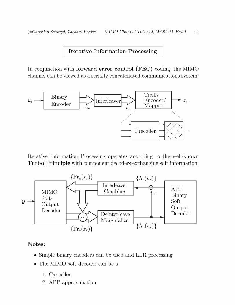
Iterative Information Processing

In conjunction with forward error control (FEC) coding, the MIMOchannel can be viewed as a serially concatenated communications system:

urvr v′r

InterleaverBinary

Encoder

TrellisEncoder/Mapper

Precoder

xr

Iterative Information Processing operates according to the well-knownTurbo Principle with component decoders exchanging soft information:

DeinterleaveMarginalize

InterleaveCombineMIMO

Soft-OutputDecoder

APPBinarySoft-OutputDecoder

y

{Λa(ur)}

{Λe(ur)}{Pra(xr)}

{Pre(xr)}

DIV

+-

Notes:

• Simple binary encoders can be used and LLR processing

• The MIMO soft decoder can be a

1. Canceller

2. APP approximation


Example: Differential Space-Time Coding

Simple differential space-time codes such as the Quaternion Code canbe used inner codes. They have simple trellis representations which canbe used by an APP decoder.

EXIT chart The figure below shows the extrinsic information transferchart of this serially concatenated systems for several binary convolutionalcodes of rate R = 2/3 bits/symbol. This chart can be used to determinethe onset of the Turbo Cliff of the system.

0

0.5

1

1.5

2

2.5

3

0 0.5 1 1.5 2 2.5 3

-1dB

-1.6dB

Parity

4-state

16-state

64-state

Ip

Ie

Dashed:Quaternion code

References:

[GrS01] A. Grant and C. Schlegel, “Differential turbo space-time coding,” Proc. IEEE Infor-mation Theory Workshop, 2001, pp. 120–122, 2001.

[ScG01] C. Schlegel and A. Grant, “Concatenated space-time coding,” IEEE Trans. Inform.Theory, to appear.


Differential Space-Time Coding: Error Performance

The error performance of this system is shown for several binary codes.It is counter-intuitive that the simple [3,2,2] parity check code shouldoutperform all stronger codes.These results agree with the predictions from the EXIT chart

Pin

ch

-off S

NR

Pin

ch

-off S

NR

Pin

ch

-off S

NR

-1.5 -1.4 -1.3 -1.2 -1.1 -1 -0.9 -0.8 -0.7 -0.610−7

10−6

10−5

10−4

10−3

10−2

10−1

1Bit Error Probability (BER)

EbN0

Parity

4-state

16-state

64-state


Iterative Detectors: Large Systems

This principle can be applied to larger systems, but their performanceis not that near-capacity anylonger. The results below are taken from[HtB01]:

2 4 6 8 10 12010

-6

10-5

10-4

10-3

10-2

10-1

100

Cap

acity

QP

SK

1.6

dB

Cap

acity

16

QA

M 3

.8dB

Cap

acity

64Q

AM

6.4

dB

QPSK16QAM 64QAM

Eb/N0 [dB]

BER 8× 8 antenna system

References:

[HtB01] B.M. Hochwald and S. tenBrink, “Achieving near-capacity on a multiple-antennachannel,” private communication, 2001, submitted IEEE Trans. Commun..

MIMO Channels and Space-Time Coding - pudn.comread.pudn.com/downloads111/doc/comm/464263/MIMO...

Documents

Transcript of MIMO Channels and Space-Time Coding - pudn.comread.pudn.com/downloads111/doc/comm/464263/MIMO...