MIMO Broadcasting for Simultaneous Wireless Information and Power Transfer
13
IEEE TRANSACTIONS ON WIRELESS COMMUNICATIONS, VOL. 12, NO. 5, MAY 2013 1989 MIMO Broadcasting for Simultaneous Wireless Information and Power Transfer Rui Zhang, Member, IEEE , and Chin Keong Ho, Member, IEEE Abstract — Wireless power transfer (WPT) is a promising new solution to provide convenient and perpetual energy supplies to wireless networks. In practice, WPT is implementable by vari- ous tech nolog ies such as induc tiv e coupl ing, magne tic res onate coupl ing, and elec tromagnet ic (EM) radi ation, for shor t-/mi d- /long-range applications, respectiv ely . In this paper , we consider the EM or radio signal enabled WPT in particular. Since radio sig nal s can carr y ene rgy as wel l as inf ormati on at the same time, a uni fied study on simultane ous wireless information and power transfer (SWIPT) is pursued . Spec ifical ly , this paper stud ies a multip le-i nput multip le-ou tput (MIMO) wire less broa dcast syste m consi sting of three nodes , wher e one rec eiv er harv ests energy and another receiver decodes information separately from the signals sent by a common transmitter, and all the transmitter and re cei vers may be equipped wit h mul tiple ant ennas. Two scen arios are exami ned, in which the info rmat ion rec eiv er and energy receiver are separated and see different MIMO channels from the transmitter, or co-located and see the identical MIMO channel from the transmitter. For the case of separated receivers, we derive the optimal transmission strategy to achieve different trade offs for maximal info rmati on rate vers us energy trans fer , whi ch ar e cha rac ter ized by the boundary of a so- calle d rate- energy (R-E) regio n. Fo r the cas e of co- loc ate d re ce iver s, we show an outer bound for the achievable R-E region due to the potential limitation that practical energy harvesting receivers are not yet able to decode information directly. Under this constraint, we inv esti gate two pract ical designs for the co-lo cate d rec eiv er case, namely time switching and power splitting, and characterize their achievable R-E regions in comparison to the outer bound. Index T erms—MIMO system, broadcas t chann el, pre codin g, wireless powe r , simultaneo us wire less info rmati on and powe r transfer (SWIPT), rate-energy tradeoff, energy harvesting. I. I NTRODUCTION E NERGY -CONS TRAINE D wireless netwo rks, such as sensor networks, are typically powered by batteries that have limited operation time. Although replacing or recharging the batteries can prolong the lifetime of the network to a certain extent, it usually incurs high costs and is inconvenient, hazardous (say, in toxic environments), or even impossible (e.g., for sensors embedded in building structures or inside human bodies). A more convenient, safer, as well as “greener” Manuscript received February 15, 2012; revised June 8, 2012 and January 3, 2013; accepted February 13, 2013. The associate editor coordinating the review of this paper and approving it for publication was M. Torlak. This paper has been presented in part at the IEEE Global Communications Conference (Globecom), December 5-9, 2011, Houston, USA. R. Zhang is with the Department of Electrical and Computer Engineering, National University of Singapore (e-mail: [email protected]). He is also with the Institute for Infocomm Research, A*STAR, Singapore. C. K. Ho is with the Institute for Infocomm Research, A*STAR, Singapor e (e-mail: hock@i2r .a-star .edu.sg). This work was supported in part by the National University of Singapore under the research grant R-263-000-679-133. Digital Object Identifier 10.1109/TWC.2013.031 813.1202 24 alternative is thus to harvest energy from the environment, which virtually provides perpetual energy supplies to wireless devices. In addition to other commonly used energy sources such as solar and wind, ambient radio-frequency (RF) signals can be a viable new source for ene rgy sca ven gin g. It is worth noting that RF-based energy harve sting is typic ally suitable for low-power applications (e.g., sensor networks), but also can be applied for scenarios with more substantial power consumptions if dedicated wireless power transmission is implemented. 1 On the other hand, since RF si gna ls tha t car ry ene rgy can at the same time be used as a vehicle for transporting information, si multane ous wir eless information and power transfer (SWIPT) becomes an interesting new area of research that attracts increasi ng atten tion. Altho ugh a unifie d stud y on this topic is still in the infancy stage, there have been notable results reported in the literature [1], [2]. In [1], Varsh- ney first proposed a capacity-energy function to characterize the fundamental tradeoffs in simu ltane ous infor mati on and energy transfer. For the single-antenna or SISO (single-input single-output) A WGN (additive white Gaussian noise) channel with amplitude-constrained inputs, it was shown in [1] that there exis t nontr ivi al trade offs in maximizing infor mati on rate versus (vs.) power transfer by optimizing the input dis- tribution. However, if the average transmit-power constraint is consi der ed ins tea d, the above two goa ls can be shown to be aligned for the SISO AWGN channel with Gaussian input signals, and thus there is no nontrivial tradeoff. In [2], Grover and Sahai extended [1] to frequency-selective single- antenna AWGN channels with the average power constraint, by sho wing that a non-t rivi al tradeoff exist s in freque ncy- domain power allocation for maximal information vs. energy transfer. As a matter of fact, wirele ss power tran sfer (WPT) or in short wir eless power , which gen era lly refer s to the trans- missions of electrical energy from a power source to one or more electrical loads without any interconnecting wires, has been investigated and implemented with a long history. Genera lly spe aki ng, WPT is car rie d out usi ng eit her the “near-field” electromagnetic (EM) induction (e.g., inductive coupli ng, capaci tiv e coupl ing) for short -dis tance (say , less than a meter) applications such as passive radio-frequency identification (RFID) [3], or the “far-field” EM radiation in the form of microwaves or lasers for long-range (up to a few kilometers) applications such as the transmissions of energy 1 Int ere ste d rea de rs may vis it the compa ny web sit e of Po wer cas t at http://www.powercastco.com/ for more information on recent applications of dedicated RF-based power transfer. 1536-1276/13$31.00 c 2013 IEEE
Transcript of MIMO Broadcasting for Simultaneous Wireless Information and Power Transfer

8/13/2019 MIMO Broadcasting for Simultaneous Wireless Information and Power Transfer
http://slidepdf.com/reader/full/mimo-broadcasting-for-simultaneous-wireless-information-and-power-transfer 1/13
IEEE TRANSACTIONS ON WIRELESS COMMUNICATIONS, VOL. 12, NO. 5, MAY 2013 1989
MIMO Broadcasting for SimultaneousWireless Information and Power Transfer
Rui Zhang, Member, IEEE , and Chin Keong Ho, Member, IEEE
Abstract— Wireless power transfer (WPT) is a promising newsolution to provide convenient and perpetual energy supplies towireless networks. In practice, WPT is implementable by vari-ous technologies such as inductive coupling, magnetic resonatecoupling, and electromagnetic (EM) radiation, for short-/mid-
/long-range applications, respectively. In this paper, we considerthe EM or radio signal enabled WPT in particular. Since radiosignals can carry energy as well as information at the sametime, a unified study on simultaneous wireless information and power transfer (SWIPT) is pursued. Specifically, this paper studiesa multiple-input multiple-output (MIMO) wireless broadcastsystem consisting of three nodes, where one receiver harvestsenergy and another receiver decodes information separately fromthe signals sent by a common transmitter, and all the transmitterand receivers may be equipped with multiple antennas. Twoscenarios are examined, in which the information receiver andenergy receiver are separated and see different MIMO channels
from the transmitter, or co-located and see the identical MIMOchannel from the transmitter. For the case of separated receivers,we derive the optimal transmission strategy to achieve differenttradeoffs for maximal information rate versus energy transfer,which are characterized by the boundary of a so-called rate-energy (R-E) region. For the case of co-located receivers, weshow an outer bound for the achievable R-E region due to thepotential limitation that practical energy harvesting receivers arenot yet able to decode information directly. Under this constraint,we investigate two practical designs for the co-located receivercase, namely time switching and power splitting, and characterizetheir achievable R-E regions in comparison to the outer bound.
Index Terms—MIMO system, broadcast channel, precoding,wireless power, simultaneous wireless information and powertransfer (SWIPT), rate-energy tradeoff, energy harvesting.
I. INTRODUCTION
ENERGY-CONSTRAINED wireless networks, such as
sensor networks, are typically powered by batteries that
have limited operation time. Although replacing or recharging
the batteries can prolong the lifetime of the network to acertain extent, it usually incurs high costs and is inconvenient,
hazardous (say, in toxic environments), or even impossible
(e.g., for sensors embedded in building structures or inside
human bodies). A more convenient, safer, as well as “greener”
Manuscript received February 15, 2012; revised June 8, 2012 and January3, 2013; accepted February 13, 2013. The associate editor coordinating thereview of this paper and approving it for publication was M. Torlak.
This paper has been presented in part at the IEEE Global CommunicationsConference (Globecom), December 5-9, 2011, Houston, USA.
R. Zhang is with the Department of Electrical and Computer Engineering,National University of Singapore (e-mail: [email protected]). He is alsowith the Institute for Infocomm Research, A*STAR, Singapore.
C. K. Ho is with the Institute for Infocomm Research, A*STAR, Singapore(e-mail: [email protected]).
This work was supported in part by the National University of Singaporeunder the research grant R-263-000-679-133.
Digital Object Identifier 10.1109/TWC.2013.031813.120224
alternative is thus to harvest energy from the environment,
which virtually provides perpetual energy supplies to wireless
devices. In addition to other commonly used energy sources
such as solar and wind, ambient radio-frequency (RF) signals
can be a viable new source for energy scavenging. It is
worth noting that RF-based energy harvesting is typically
suitable for low-power applications (e.g., sensor networks),
but also can be applied for scenarios with more substantialpower consumptions if dedicated wireless power transmission
is implemented.1
On the other hand, since RF signals that carry energy
can at the same time be used as a vehicle for transportinginformation, simultaneous wireless information and power
transfer (SWIPT) becomes an interesting new area of research
that attracts increasing attention. Although a unified study
on this topic is still in the infancy stage, there have beennotable results reported in the literature [1], [2]. In [1], Varsh-
ney first proposed a capacity-energy function to characterizethe fundamental tradeoffs in simultaneous information and
energy transfer. For the single-antenna or SISO (single-input
single-output) AWGN (additive white Gaussian noise) channel
with amplitude-constrained inputs, it was shown in [1] that
there exist nontrivial tradeoffs in maximizing information
rate versus (vs.) power transfer by optimizing the input dis-
tribution. However, if the average transmit-power constraintis considered instead, the above two goals can be shownto be aligned for the SISO AWGN channel with Gaussian
input signals, and thus there is no nontrivial tradeoff. In [2],
Grover and Sahai extended [1] to frequency-selective single-
antenna AWGN channels with the average power constraint,
by showing that a non-trivial tradeoff exists in frequency-
domain power allocation for maximal information vs. energy
transfer.
As a matter of fact, wireless power transfer (WPT) or in
short wireless power , which generally refers to the trans-
missions of electrical energy from a power source to one
or more electrical loads without any interconnecting wires,
has been investigated and implemented with a long history.Generally speaking, WPT is carried out using either the
“near-field” electromagnetic (EM) induction (e.g., inductive
coupling, capacitive coupling) for short-distance (say, less
than a meter) applications such as passive radio-frequency
identification (RFID) [3], or the “far-field” EM radiation inthe form of microwaves or lasers for long-range (up to a few
kilometers) applications such as the transmissions of energy
1Interested readers may visit the company website of Powercast athttp://www.powercastco.com/ for more information on recent applications of dedicated RF-based power transfer.
1536-1276/13$31.00 c 2013 IEEE

8/13/2019 MIMO Broadcasting for Simultaneous Wireless Information and Power Transfer
http://slidepdf.com/reader/full/mimo-broadcasting-for-simultaneous-wireless-information-and-power-transfer 2/13
1990 IEEE TRANSACTIONS ON WIRELESS COMMUNICATIONS, VOL. 12, NO. 5, MAY 2013
Energy Flow
Information Flow
Access Point
User Terminals
Fig. 1. A wireless network with dual information and energy transfer.
from orbiting solar power satellites to Earth or spacecrafts
[4]. However, prior research on EM radiation based WPT, in
particular over the RF band, has been pursued independently
from that on wireless information transfer (WIT) or radio
communication. This is non-surprising since these two lines of
work in general have very different research goals: WIT is to
maximize the information transmission capacity of wirelesschannels subject to channel impairments such as the fading
and receiver noise, while WPT is to maximize the energy
transmission efficiency (defined as the ratio of the energy
harvested and stored at the receiver to that consumed by
the transmitter) over a wireless medium. Nevertheless, it is
worth noting that the design objectives for WPT and WIT
systems can be aligned, since given a transmitter energy
budget, maximizing the signal power received (for WPT) is
also beneficial in maximizing the channel capacity (for WIT)
against the receiver noise.
Hence, in this paper we attempt to pursue a unified study onWIT and WPT for emerging wireless applications with such a
dual usage. An example of such wireless dual networks is en-
visaged in Fig. 1, where a fixed access point (AP) coordinatesthe two-way communications to/from a set of distributed user
terminals (UTs). However, unlike the conventional wireless
network in which both the AP and UTs draw energy from
constant power supplies (by e.g. connecting to the grid or
a battery), in our model, only the AP is assumed to have a
constant power source, while all UTs need to replenish energyfrom the received signals sent by the AP via the far-field
RF-based WPT. Consequently, the AP needs to coordinatethe wireless information and energy transfer to UTs in the
downlink, in addition to the information transfer from UTs inthe uplink. Wireless networks with such a dual information
and power transfer feature have not yet been studied in
the literature to our best knowledge, although some of their
interesting applications have already appeared in, e.g., the
body sensor networks [5] with the out-body local processing
units (LPUs) powered by battery communicating and at the
same time sending wireless power to in-body sensors that have
no embedded power supplies. However, how to characterize
the fundamental information-energy transmission tradeoff insuch dual networks is still an open problem.
In this paper, we focus our study on the downlink case
with simultaneous WIT and WPT from the AP to UTs. In the
generic system model depicted in Fig. 1, each UT can in gen-
eral harvest energy and decode information at the same time
(by e.g. applying the power splitting scheme introduced later
in this paper). However, from an implementation viewpoint,
one particular design whereby each UT operates as either an
information receiver or an energy receiver at any given timemay be desirable, which is referred to as time switching. This
scheme is practically appealing since state-of-the-art wirelessinformation and energy receivers are typically designed to
operate separately with very different power sensitivities (e.g.,
−50dBm for information receivers vs. −10dBm for energy
receivers). As a result, if time switching is employed at each
UT jointly with the “near-far” based transmission scheduling
at the AP, i.e., UTs that are close to the AP and thus receivehigh power from the AP are scheduled for WET, whereas those
that are more distant from the AP and thus receive lower powerare scheduled for WIT, then SWIPT systems can be efficiently
implemented with existing information and energy receivers
and the additional time-switching device at each receiver.
For an initial study on SWIPT, this paper considers the
simplified scenarios with only one or two active UTs in thenetwork at any given time. For the case of two UTs, we assume
time switching, i.e., the two UTs take turns to receive energy
or (independent) information from the AP over different time
blocks. As a result, when one UT receives information fromthe AP, the other UT can opportunistically harvest energy from
the same signal broadcast by the AP, and vice versa. Hence,at each block, one UT operates as an information decoding
(ID) receiver, and the other UT as an energy harvesting (EH)
receiver. We thus refer to this case as separated EH and ID
receivers. On the other hand, for the case with only one single
UT to be active at one time (while all other UTs are assumed
to be in the off/sleep mode), the active UT needs to harvest
energy as well as decode information from the same signalsent by the AP, i.e., the same set of receiving antennas areshared by both EH and ID receivers residing in the same
UT. Thus, this case is referred to as co-located EH and ID
receivers. Surprisingly, as we will show later in this paper,
the optimal information-energy tradeoff for the case of co-
located receivers is more challenging to characterize than that
for the case of separated receivers, due to a potential limitation
that practical EH receiver circuits are not yet able to decode
the information directly and vice versa. Note that similar to
the case of separated receives, time switching can also be
applied in the case of co-located receivers to orthogonalize
the information and energy transmissions at each receiving
antenna; however, this scheme is in general suboptimal forthe achievable rate-energy tradeoffs in the case of co-located
receivers, as will be shown later in this paper.
Some further assumptions are made in this paper for the pur-
pose of exposition. Firstly, this paper considers a quasi-static
fading environment where the wireless channel between the
AP and each UT is assumed to be constant over a sufficiently
long period of time during which the number of transmitted
symbols can be approximately regarded as being infinitely
large. Under this assumption, we further assume that it is
feasible for each UT to estimate the downlink channel fromthe AP and then send it back to the AP via the uplink, since
the time overhead for such channel estimation and feedback is

8/13/2019 MIMO Broadcasting for Simultaneous Wireless Information and Power Transfer
http://slidepdf.com/reader/full/mimo-broadcasting-for-simultaneous-wireless-information-and-power-transfer 3/13
ZHANG and HO: MIMO BROADCASTING FOR SIMULTANEOUS WIRELESS INFORMATION AND POWER TRANSFER 1991
Energy Receiver
Transmitter
Information Receiver
Fig. 2. A MIMO broadcast system for simultaneous wireless informationand power transfer.
a negligible portion of the total transmission time due to quasi-
static fading. We will address the more general case of fading
channels with imperfect/partial channel knowledge at thetransmitter in our future work. Secondly, we assume that the
system under our study typically operates at the high signal-to-noise ratio (SNR) regime for the ID receiver in the case of co-
located receivers. This is to be compatible with the high-power
operating requirement for the EH receiver of practical interest
as previously mentioned. Thirdly, without loss of generality,
we assume a multi-antenna or MIMO (multiple-input multiple-
output) system, in which the AP is equipped with multipleantennas, and each UT is equipped with one or more antennas,
for enabling both the high-performance wireless energy andinformation transmissions (as it is well known that for WIT
only, MIMO systems can achieve folded array/capacity gainsover SISO systems by spatial beamforming/multiplexing [6]).
Under the above assumptions, a three-node MIMO broad-
cast system is considered in this paper, as shown in Fig. 2,
wherein the EH and ID receivers harvest energy and decode
information separately from the signal sent by a common
transmitter. Note that this system model refers to the case
of separated EH and ID receivers in general, but includes
the co-located receivers as a special case when the MIMO
channels from the transmitter to both receivers become iden-
tical. Assuming this model, the main results of this paper are
summarized as follows:
• For the case of separated EH and ID receivers, we
design the optimal transmission strategy to achieve dif-ferent tradeoffs between maximal information rate vs.
energy transfer, which are characterized by the boundary
of a so-called rate-energy (R-E) region. We derive a
semi-closed-form expression for the optimal transmit
covariance matrix (for the joint precoding and power
allocation) to achieve different rate-energy pairs on the
boundary of the R-E region. Note that the R-E region is
a multiuser extension of the single-user capacity-energy
function in [1]. Also note that the multi-antenna broadcast
channel (BC) has been investigated in e.g. [7]–[12] forinformation transfer solely by unicasting or multicasting.
However, MIMO-BC for SWIPT as considered in this
Energy
Harvester
Energy
Harvester
Information
Decoder
Information
Decoder
Fig. 3. Two practical designs for the co-located energy and informationreceivers, which are applied for each receiving antenna.
paper is new and has not yet been studied by any prior
work.
• For the case of co-located EH and ID receivers, we
show that the proposed solution for the case of separatedreceivers is also applicable with the identical MIMO
channel from the transmitter to both ID and EH receivers.
Furthermore, we consider a potential practical constraintthat EH receiver circuits cannot directly decode the
information (i.e., any information embedded in receivedsignals sent to the EH receiver is lost during the EH
process). Under this constraint, we show that the R-E
region with the optimal transmit covariance (obtained
without such a constraint) in general only serves as a
performance outer bound for the co-located receiver case.
• Hence, we investigate two practical receiver designs,namely time switching and power splitting, for the case
of co-located receivers. As shown in Fig. 3, for timeswitching, each receiving antenna periodically switches
between the EH receiver and ID receiver, whereas for
power splitting, the received signal at each antenna is
split into two separate signal streams with different power
levels, one sent to the EH receiver and the other to the ID
receiver. Note that time switching has also been proposedin [14] for the SISO AWGN channel. Furthermore, note
that the antenna switching scheme whereby the receiving
antennas are divided into two groups with one group
switched to information decoding and the other group
to energy harvesting can be regarded as a special case
of power splitting with only binary splitting power ratios
at each receiving antenna. For these practical receiver
designs, we derive their achievable R-E regions as com-
pared to the R-E region outer bound, and characterizethe conditions under which their performance gaps can
be closed. For example, we show that the power splittingscheme approaches the tradeoff upper bound asymptot-
ically when the RF-band antenna noise at the receiverbecomes more dominant over the baseband processing
noise (more details are given in Section IV-C).
The rest of this paper is organized as follows: Section
II presents the system model, characterizes the rate-energy
region, and formulates the problem for finding the optimal
transmit covariance matrix. Section III presents the opti-mal transmit covariance solution for the case of separated
receivers. Section IV extends the solution to the case of

8/13/2019 MIMO Broadcasting for Simultaneous Wireless Information and Power Transfer
http://slidepdf.com/reader/full/mimo-broadcasting-for-simultaneous-wireless-information-and-power-transfer 4/13
1992 IEEE TRANSACTIONS ON WIRELESS COMMUNICATIONS, VOL. 12, NO. 5, MAY 2013
co-located receivers to obtain a performance upper bound,
proposes practical receiver designs, and analyzes their perfor-
mance limits as compared to the performance upper bound.
Finally, Section V concludes the paper and provides some
promising directions for future work.
Notation: For a square matrix S , tr(S ), |S |, S −1, and S 1
2
denote its trace, determinant, inverse, and square-root, respec-
tively, while S
0 and S
0 mean that S is positive semi-
definite and positive definite, respectively. For an arbitrary-size
matrix M , M H and M T denote the conjugate transpose and
transpose of M , respectively. diag(x1, . . . , xM ) denotes anM × M diagonal matrix with x1, . . . , xM being the diagonal
elements. I and 0 denote an identity matrix and an all-zero
vector, respectively, with appropriate dimensions. E[·] denotes
the statistical expectation. The distribution of a circularly
symmetric complex Gaussian (CSCG) random vector withmean x and covariance matrix Σ is denoted by CN (x,Σ),
and ∼ stands for “distributed as”. Cx×y denotes the space of x × y matrices with complex entries. z is the Euclidean
norm of a complex vector z, and |z| is the absolute value
of a complex scalar z. max(x, y) and min(x, y) denote themaximum and minimum between two real numbers, x and y ,
respectively, and (x)+ = max(x, 0). All the log(·) functions
have base-2 by default.
II . SYSTEM MODEL AND PROBLEM FORMULATION
As shown in Fig. 2, this paper considers a wireless broadcastsystem consisting of one transmitter, one EH receiver, and
one ID receiver. It is assumed that the transmitter is equipped
with M ≥ 1 transmitting antennas, and the EH receiver and
the ID receiver are equipped with N EH ≥ 1 and N ID ≥ 1receiving antennas, respectively. In addition, it is assumed
that the transmitter and both receivers operate over the same
frequency band. Assuming a narrow-band transmission over
quasi-static fading channels, the baseband equivalent channels
from the transmitter to the EH receiver and ID receiver can
be modeled by matrices G ∈ CN EH×M and H ∈ CN ID×M ,
respectively. It is assumed that at each fading state, G andH are both known at the transmitter, and separately known
at the corresponding receiver. Note that for the case of co-
located EH and ID receivers, G is identical to H and thusN EH = N ID.
It is worth noting that the EH receiver does not need toconvert the received signal from the RF band to the baseband
in order to harvest the carried energy. Nevertheless, thanks to
the law of energy conservation, it can be assumed that the totalharvested RF-band power (energy normalized by the baseband
symbol period), denoted by Q, from all receiving antennas at
the EH receiver is proportional to that of the received baseband
signal, i.e.,
Q = ζ E[Gx(n)2] (1)
where ζ is a constant that accounts for the loss in the energy
transducer for converting the harvested energy to electrical
energy to be stored; for the convenience of analysis, it is
assumed that ζ = 1 in this paper unless stated otherwise. Weuse x(n) ∈ CM ×1 to denote the baseband signal broadcast by
the transmitter at the nth symbol interval, which is assumed to
be random over n, without loss of generality. The expectation
in (1) is thus used to compute the average power harvested by
the EH receiver at each fading state. Note that for simplicity,
we assumed in (1) that the harvested energy due to the
background noise at the EH receiver is negligible and thus
can be ignored.2
On the other hand, the baseband transmission from the
transmitter to the ID receiver can be modeled by
y(n) = Hx(n) + z(n) (2)
where y(n) ∈ CN ID×1 denotes the received signal at the nth
symbol interval, and z(n) ∈ CN ID×1 denotes the receiver
noise vector. It is assumed that z(n)’s are independent over
n and z(n) ∼ CN (0, I ). Under the assumption that x(n)is random over n, we use S = E[x(n)xH (n)] to denote the
covariance matrix of x(n). In addition, we assume that there is
an average power constraint at the transmitter across all trans-
mitting antennas denoted by E[x(n)2] = tr(S ) ≤ P . In
the following, we examine the optimal transmit covariance S
to maximize the transported energy efficiency and information
rate to the EH and ID receivers, respectively.Consider first the MIMO link from the transmitter to the
EH receiver when the ID receiver is not present. In this
case, the design objective for S is to maximize the powerQ received at the EH receiver. Since from (1) it follows that
Q = tr(GSGH ) with ζ = 1, the aforementioned design
problem can be formulated as
(P1) max
S Q := tr
GSGH
s.t. tr(S ) ≤ P,S 0.
Let T 1 = min(M, N EH) and the (reduced) singular value
decomposition (SVD) of G be denoted by G = U GΓ1/2G V
H G ,
where U G ∈ C
N EH×T 1
and V G ∈ C
M ×T 1
, each of which consists of orthogonal columns with unit norm, andΓG = diag(g1, . . . , gT 1) with g1 ≥ g2 ≥ . . . ≥ gT 1 ≥ 0.
Furthermore, let v1 denote the first column of V G. Then, we
have the following proposition.Proposition 2.1: The optimal solution to (P1) is S EH =
P v1vH 1 .Proof: The proof follows directly by examining the SVD
of S , and is thus omitted here for brevity. Please refer to alonger version of this paper [23] for the complete proof.
Given S = S EH, it follows that the maximum harvestedpower at the EH receiver is given by Qmax = g1P . It
is worth noting that since S EH is a rank-one matrix, the
maximum harvested power is achieved by beamforming at thetransmitter, which aligns with the strongest eigenmode of the
matrix GH G, i.e., the transmitted signal can be written as
x(n) =√
P v1s(n), where s(n) is an arbitrary random signalover n with zero mean and unit variance, and v1 is the transmit
beamforming vector. For convenience, we name the abovetransmit beamforming scheme to maximize the efficiency of
WPT as “energy beamforming”.Next, consider the MIMO link from the transmitter to
the ID receiver without the presence of any EH receiver.
2The results of this paper are readily extendible to study the impacts of non-negligible background noise and/or co-channel interference on the SWIPTsystem performance.

8/13/2019 MIMO Broadcasting for Simultaneous Wireless Information and Power Transfer
http://slidepdf.com/reader/full/mimo-broadcasting-for-simultaneous-wireless-information-and-power-transfer 5/13
ZHANG and HO: MIMO BROADCASTING FOR SIMULTANEOUS WIRELESS INFORMATION AND POWER TRANSFER 1993
Assuming the optimal Gaussian codebook at the transmitter,
i.e., x(n) ∼ CN (0,S ), the transmit covarianceS to maximize
the transmission rate over this MIMO channel can be obtained
by solving the following problem [13]:
(P2) max
S R := log |I + HSH H |
s.t. tr(S ) ≤ P,S 0.
The optimal solution to the above problem is known tohave the following form [13]: S ID = V H ΛV
H H , where
V H ∈ CM ×T 2 is obtained from the (reduced) SVD of H
expressed by H = U H Γ1/2H V
H H , with T 2 = min(M, N ID),
U H ∈ CN ID×T 2 , ΓH = diag(h1, . . . , hT 2), h1 ≥ h2 ≥
. . . ≥ hT 2 ≥ 0, and Λ = diag( p1, . . . , pT 2) with the
diagonal elements obtained from the standard “water-filling
(WF)” power allocation solution [13]:
pi =
ν − 1
hi
+, i = 1, . . . , T 2 (3)
with ν being the so-called (constant) water-level that makes
T 2
i=1
pi = P . The corresponding maximum transmission rate
is then given by Rmax =
T 2i=1 log(1 + hi pi). The maximum
rate is achieved in general by spatial multiplexing [6] overup to T 2 spatially decoupled AWGN channels, together with
the Gaussian codebook, i.e., the transmitted signal can beexpressed as x(n) = V H Λ
1/2s(n), where s(n) is a Gaus-
sian random vector ∼ CN (0, I ), V H and Λ1/2 denote the
precoding matrix and the (diagonal) power allocation matrix,
respectively. Remark 2.1: It is worth noting that in Problem (P1), it
is assumed that the transmitter sends to the EH receiver
continuously. Now suppose that the transmitter only transmits
a fraction of the total time denoted by α with 0 < α ≤ 1.
Furthermore, assume that the transmit power level can beadjusted flexibly provided that the consumed average power is
bounded by P , i.e., α·tr(S )+(1−α)·0 ≤ P or tr(S ) ≤ P/α.
In this case, it can be easily shown that the transmit covariance
S = (P/α)v1vH 1 also achieves the maximum harvested power
Qmax = g1P for any 0 < α ≤ 1, which suggests that
the maximum power delivered is independent of transmission
time. However, unlike the case of maximum power transfer,
the maximum information rate reliably transmitted to the ID
receiver requires that the transmitter send signals continuously,
i.e., α = 1, as assumed in Problem (P2). This can be easily
verified by observing that for any 0 < α ≤ 1 and S 0,
α log |I + H (S /α)H H | ≤ log |I + HSH H | where the
equality holds only when α = 1, since R is a nonlinearconcave function of S . Thus, to maximize both power and rate
transfer at the same time, the transmitter should broadcast to
the EH and ID receivers all the time. Furthermore, note that
the assumed Gaussian distribution for transmitted signals is
necessary for achieving the maximum rate transfer, but not
necessary for the maximum power transfer. In fact, for any
arbitrary complex number c that satisfies |c| = 1, even a deter-
ministic transmitted signal x(n) =√
P v1c, ∀n, achieves the
maximum transferred power Qmax in Problem (P1). However,
to maximize simultaneous power and information transfer withthe same transmitted signal, the Gaussian input distribution is
sufficient as well as necessary.
0 50 100 150 200 2500
0.1
0.2
0.3
0.4
0.5
0.6
0.7
Rate (Mbps)
E n e r g y
( m W )
Optimal Transmit Covariance
Time−Sharing
(REH
, Qmax
)
(Rmax
, QID
)
Fig. 4. Rate-energy tradeoff for a MIMO broadcast system with separatedEH and ID receivers, and M = N EH = N ID = 4.
Now, consider the case where both the EH and ID receivers
are present. From the above results, it is seen that theoptimal transmission strategies for maximal power transfer
and information transfer are in general different, which are
energy beamforming and information spatial multiplexing,
respectively. It thus motivates our investigation of the fol-
lowing question: What is the optimal broadcasting strategy
for simultaneous wireless power and information transfer? To
answer this question, we propose to use the Rate-Energy (R-E)
region (defined below) to characterize all the achievable rate
(in bits/sec/Hz or bps for information transfer) and energy
(in joule/sec or watt for power transfer) pairs under a given
transmit power constraint. Without loss of generality, assumingthat the transmitter sends Gaussian signals continuously (cf.
Remark 2.1), the R-E region is defined as
CR−E(P )
(R, Q) : R ≤ log |I + HSH H |,
Q ≤ tr(GSGH ), tr(S ) ≤ P,S 0
. (4)
In Fig. 4, an example of the above defined R-E region
(see Section III for the algorithm to compute the boundary
of this region) is shown for a practical MIMO broadcast
system with separated EH and ID receivers (i.e., G = H ).It is assumed that M = N EH = N ID = 4. The transmitter
power is assumed to be P = 1 watt(W) or 30dBm. Thedistances from the transmitter to the EH and ID receivers
are assumed to be 1 meter and 10 meters, respectively; thus,
we can exploit the near-far based energy and information
transmission scheduling, which may correspond to, e.g., a
dedicated energy transfer system (to “near” users) with op-
portunistic information transmission (to “far” users), or vice
versa. Assuming a carrier frequency of f c = 900MHz and the
power pathloss exponent to be 4, the distance-dependent signal
attenuation from the AP to EH/ID receiver can be estimated
as 40dB and 80dB, respectively. Accordingly, the averagesignal power at the EH/ID receiver is thus 30dBm−40dB=
−10dBm and 30dBm
−80dB=
−50dBm, respectively. It is

8/13/2019 MIMO Broadcasting for Simultaneous Wireless Information and Power Transfer
http://slidepdf.com/reader/full/mimo-broadcasting-for-simultaneous-wireless-information-and-power-transfer 6/13
1994 IEEE TRANSACTIONS ON WIRELESS COMMUNICATIONS, VOL. 12, NO. 5, MAY 2013
further assumed that in addition to signal pathloss, Rayleigh
fading is present, as such each element of channel matrices
G and H is independently drawn from the CSCG distribution
with zero mean and variance −10dBm (for EH receiver) and
−50dBm for (for ID receiver), respectively (to be consistent
with the signal pathloss previously assumed). Furthermore,the bandwidth of the transmitted signal is assumed to be
10MHz, while the receiver noise is assumed to be whiteGaussian with power spectral density −140dBm/Hz (which
is dominated by the receiver processing noise rather than
the background thermal noise) or average power −70dBm
over the bandwidth of 10MHz. As a result, considering all
of transmit power, signal attenuation, fading and receiver
noise, the per-antenna average SNR at the ID receiver isequal to 30 − 80 − (−70) = 20dB, which corresponds to
P = 100 in the equivalent signal model for the ID receivergiven in (2) with unit-norm noise. In addition, we assume
that for the EH receiver, the energy conversion efficiency isζ =50%. Considering this together with transmit power and
signal attenuation, the average per-antenna signal power at the
EH receiver is thus 0.5×(30dBm−40dB) = 50µW.From Fig. 4, it is observed that with energy beamforming,
the maximum harvested energy rate for the EH receiver is
around Qmax = 0.57mW, while with spatial multiplexing,
the maximum information rate for the ID receiver is around
Rmax = 225Mbps. It is easy to identify two boundary pointsof this R-E region denoted by (REH, Qmax) and (Rmax, QID),
respectively. For the former boundary point, the transmit co-variance is S EH, which corresponds to transmit beamforming
and achieves the maximum transferred power Qmax to the
EH receiver, while the resulting information rate for the ID
receiver is given by REH = log(1+ Hv12P ). On the other
hand, for the latter boundary point, the transmit covariance is
S ID, which corresponds to transmit spatial multiplexing andachieves the maximum information rate transferred to the ID
receiver Rmax, while the resulting power transferred to the
EH receiver is given by QID = tr(GS IDGH ).
Since the optimal tradeoff between the maximum energyand information transfer rates is characterized by the boundary
of the R-E region, it is important to characterize all theboundary rate-power pairs of CR−E(P ) for any P > 0. From
Fig. 4, it is easy to observe that if R ≤ REH, the maximum
harvested power Qmax is achievable with the same transmit
covariance that achieves the rate-power pair (REH, Qmax);
similarly, the maximum information rate Rmax is achievable
provided that Q
≤ QID. Thus, the remaining boundary
of CR−E(P ) yet to be characterized is over the intervals:REH < R < Rmax, QID < Q < Qmax. We thus considerthe following optimization problem:
(P3) max
S logI + HSH H
s.t. tr
GSGH
≥ Q, tr(S ) ≤ P, S 0.
Note that if Q takes values from QID < Q < Qmax, the
corresponding optimal rate solutions of the above problems
are the boundary rate points of the R-E region over REH <R < Rmax. Notice that the transmit covariance solutions to
the above problems in general yield larger rate-power pairs
than those by simply “time-sharing” the optimal transmit
covariance matrices S EH and S ID for EH and ID receivers
separately (see the dashed line in Fig. 4).3
Problem (P3) is a convex optimization problem, since its
objective function is concave over S and its constraints specify
a convex set of S . Note that (P3) resembles a similar problemformulated in [15], [16] (see also [17] and references therein)
under the cognitive radio (CR) setup, where the rate of asecondary MIMO link is maximized subject to a set of so-
called interference power constraints to protect the co-channel
primary receivers. However, there is a key difference between
(P3) and the problem in [16]: the harvested power constraint
in (P3) has the reversed inequality of that of the interference
power constraint in [16], since in our case it is desirable for
the EH receiver to harvest more power from the transmitter, as
opposed to that in [16] the interference power at the primary
receiver should be minimized. As such, it is not immediatelyclear whether the solution in [16] can be directly applied
for solving (P3) with the reversed power inequality. In thefollowing, we will examine the solutions to Problem (P3) for
the two cases with arbitrary G and H (the case of separatedreceivers) and G = H (the case of co-located receivers),
respectively.
III. SEPARATED RECEIVERS
Consider the case where the EH receiver and ID receiver
are spatially separated and thus in general have different
channels from the transmitter. In this section, we first solve
Problem (P3) with arbitrary G and H and derive a semi-
closed-form expression for the optimal transmit covariance.
Then, we examine the optimal solution for the special case of
MISO channels from the transmitter to ID and/or EH receivers.
Since Problem (P3) is convex and satisfies the Slater’s
condition [18], it has a zero duality gap and thus can be solved
using the Lagrange duality method.4 Thus, we introduce two
non-negative dual variables, λ and µ, associated with the
harvested power constraint and transmit power constraint in
(P3), respectively. The optimal solution to Problem (P3) is
then given by the following theorem in terms of λ∗ and µ∗,
which are the optimal dual solutions of Problem (P3) (see
Appendix A for details). Note that for Problem (P3), given
any pair of Q (QID < Q < Qmax) and P > 0, there exists
one unique pair of λ∗ > 0 and µ∗ > 0.
Theorem 3.1: The optimal solution to Problem (P3) has the
following form:
S ∗ = A−1/2V ΛV H A−1/2 (5)
where A = µ∗I − λ∗GH G, V ∈ CM ×T 2 is obtained
from the (reduced) SVD of the matrix HA−1/2 given by
HA−1/2 = U Γ1/2V
H , with Γ = diag(h1, . . . , hT 2), h1 ≥
3By time-sharing, we mean that the AP transmits simultaneously to both EHand ID receivers with the energy-maximizing transmit covariance S EH (i.e.energy beamforming) for β portion of each block time, and the information-rate-maximizing transmit covariance S ID (i.e. spatial multiplexing) for theremaining 1 − β portion of each block time, with 0 ≤ β ≤ 1.
4It is worth noting that Problem (P3) is convex and thus can be solvedefficiently by the interior point method [18]; in this paper, we apply theLagrange duality method for this problem mainly to reveal the optimalprecoder structure.

8/13/2019 MIMO Broadcasting for Simultaneous Wireless Information and Power Transfer
http://slidepdf.com/reader/full/mimo-broadcasting-for-simultaneous-wireless-information-and-power-transfer 7/13
ZHANG and HO: MIMO BROADCASTING FOR SIMULTANEOUS WIRELESS INFORMATION AND POWER TRANSFER 1995
h2 ≥ . . . ≥ hT 2 ≥ 0, and Λ = diag(˜ p1, . . . , ˜ pT 2), with
˜ pi = (1 − 1/hi)+, i = 1, . . . , T 2.
Proof: See Appendix A.Note that this theorem requires that A = µ∗I −λ∗GH G 0,
implying that µ∗ > λ∗g1 (recall that g1 is the largest
eigenvalue of matrixGH G), which is not present for a similar
result in [17] under the CR setup with the reversed interference
power constraint. One algorithm that can be used to solve (P3)
is provided in Table I of Appendix A. From Theorem 3.1, the
maximum transmission rate for Problem (P3) can be shown
to be R∗ = logI + HS ∗H H
= T 2
i=1 log(1 + hi˜ pi), for
which the proof is omitted here for brevity.Next, we examine the optimal solution to Problem (P3) for
the special case where the ID receiver has one single antenna,
i.e., N ID = 1, and thus the MIMO channel H reduces to arow vector hH with h ∈ C
M ×1. Suppose that the EH receiver
is still equipped with N EH ≥ 1 antennas, and thus the MIMO
channel G remains unchanged. From Theorem 3.1, we obtainthe following corollary (see [23] for the proof).
Corollary 3.1: In the case of MISO channel from the
transmitter to ID receiver, i.e., H ≡ h
H
, the optimal solutionto Problem (P3) reduces to the following form:
S ∗ = A−1h
1
A−1/2h2 − 1
A−1/2h4
+hH A−1 (6)
where A = µ∗I − λ∗GH G, with λ∗ and µ∗ denoting the
optimal dual solutions of Problem (P3). Correspondingly, the
optimal value of (P3) is R∗ =
2logA−1/2h
+.
From (6), it is observed that the optimal transmit covariance
is a rank-one matrix, from which it follows that beamforming
is the optimal transmission strategy in this case, where the
transmit beamforming vector should be aligned with the vector
A−1
h. Moreover, consider the case where both channels fromthe transmitter to ID/EH receivers are MISO, i.e., H ≡ hH ,and G ≡ gH with g ∈ CM ×1. From Corollary 3.1, it follows
immediately that the optimal covariance solution to Problem(P3) is still beamforming. In the following theorem, we show
a closed-form solution of the optimal beamforming vector atthe transmitter for this special case, which differs from the
semi-closed-form solution (6) that was expressed in terms of
dual variables.Theorem 3.2: In the case of MISO channels from transmit-
ter to both ID and EH receivers, i.e., H ≡ hH , and G ≡ gH ,
the optimal solution to Problem (P3) can be expressed as
S ∗ = P vvH , where the beamforming vector v has a unit-
norm and is given by
v =
h 0 ≤ Q ≤ |gH h|2P QP g2 ej∠αgh g
+
1 − QP g2 hg⊥ |gH h|2P < Q ≤ P g2
(7)
where h = h/h, g = g/g, hg⊥ = hg⊥/hg⊥ with
hg⊥ = h − (gH h)g, and αgh = gH h with ∠αgh ∈ [0, 2π)denoting the phase of complex number αgh. Correspondingly,
the optimal value of (P3) is given in (8) shown at the top of
the next page.Proof: The proof is similar to that of Theorem 2 in [16],
and is thus omitted for brevity.
0 0.5 1 1.5 2 2.5 3 3.50
1
2
3
4
5
6
7
8
9
10
11
Rate (bits/channel use)
E n e r g y U
n i t
ρ=0.9
ρ=0.5
ρ=0.1
Fig. 5. Rate-energy tradeoff for a MISO broadcast system with correlatedMISO channels to the (separated) EH and ID receivers.
It is worth noting that in (7), if Q ≤ |gH h|2P , the optimal
transmit beamforming vector is based on the principle of
maximal-ratio-combining (MRC) with respect to the MISO
channel hH from the transmitter to the ID receiver, and in
this case, the harvested power constraint in Problem (P3) is
indeed not active; however, when Q > |gH h|2P , the optimal
beamforming vector is a linear combination of the two vectors
g and hg⊥ , and the combining coefficients are designed suchthat the harvested power constraint is satisfied with equality.
In Fig. 5, we show the achievable R-E regions for the caseof MISO channels from the transmitter to both EH and ID
receivers. We set P = 10. For the purpose of exposition,
it is assumed that h = g = 1 and |αgh|2
= ρ, with0 ≤ ρ ≤ 1 denoting the correlation between the two unit-
norm vectors h and g. This channel setup may correspond
to the practical scenario where the EH and ID receivers areequipped at a single device (but still physically separated), and
as a result their respective MISO channels from the transmitterhave the same power gain but are spatially correlated due
to the insufficient spacing between two separate receiving
antennas. From Theorem 3.2, the R-E regions for the three
cases of ρ = 0.1, 0.5, and 0.9 are obtained, as shown in
Fig. 5. Interestingly, it is observed that increasing ρ enlarges
the achievable R-E region, which indicates that the antenna
correlation between the EH and ID receivers can be a bene-
ficial factor for simultaneous information and power transfer.Note that in this figure, we express energy and rate in terms
of energy unit and bits/channel use, respectively, since their
practical values can be obtained by appropriate scaling basedon the realistic system parameters as for Fig. 4.
IV. CO-LOCATED RECEIVERS
In this section, we address the case where the EH and ID
receivers are co-located, and thus possess the same channel
from the transmitter, i.e., G = H and thus N EH = N ID N .We first examine the optimal solution of Problem (P3) for thiscase, from which we obtain an outer bound for the achievable
rate-power pairs in the R-E region. Then, we propose two

8/13/2019 MIMO Broadcasting for Simultaneous Wireless Information and Power Transfer
http://slidepdf.com/reader/full/mimo-broadcasting-for-simultaneous-wireless-information-and-power-transfer 8/13
1996 IEEE TRANSACTIONS ON WIRELESS COMMUNICATIONS, VOL. 12, NO. 5, MAY 2013
R∗ =
log(1 + h2P ) 0 ≤ Q ≤ |gH h|2P
log
1 +
Qg2 |αgh| +
P − Q
g2 h2 − |αgh|2
2 |gH h|2P < Q ≤ P g2.
(8)
practical receiver designs, namely time switching and powersplitting, derive their optimal transmission strategies to maxi-
mize the achievable rate-power pairs, and finally compare theresults to the R-E region outer bound.
A. Performance Outer Bound
Consider Problem (P3) with G = H . Recall that the
(reduced) SVD of H is given by H = U H Γ1/2H V
H H , with
ΓH = diag(h1, . . . , hT 2), h1 ≥ h2 ≥ . . . ≥ hT 2 ≥ 0, andT 2 = min(M, N ). From Theorem 3.1, we obtain the following
corollary (see [23] for the proof).
Corollary 4.1: In the case of co-located EH and ID re-
ceivers with G = H , the optimal solution to Problem (P3) has
the form of S ∗ = V H ΣV H H , where Σ = diag(ˆ p1, . . . , ˆ pT 2)
with the diagonal elements obtained from the following mod-ified WF power allocation:
ˆ pi =
1
µ∗ − λ∗hi− 1
hi
+, i = 1, . . . , T 2 (9)
with λ∗ and µ∗ denoting the optimal dual solutions of Problem
(P3), µ∗ > λ∗h1. The corresponding maximum transmission
rate is R∗ =T 2
i=1 log(1 + hiˆ pi).
The algorithm in Table I for solving Problem (P3) witharbitrary G and H can be simplified to solve the special case
with G = H . Corollary 4.1 reveals that for Problem (P3) in
the case of G = H , the optimal transmission strategy is in
general still spatial multiplexing over the eigenmodes of the
MIMO channel H as for Problem (P2), while the optimaltradeoffs between information transfer and power transfer are
achieved by varying the power levels allocated into different
eigenmodes, as shown in (9). It is interesting to observe that
the power allocation in (9) reduces to the conventional WF
solution in (3) with a constant water-level when λ∗ = 0, i.e.,
the harvested power constraint in Problem (P3) is inactive withthe optimal power allocation. However, when λ∗ > 0 and thus
the harvested power constraint is active corresponding to the
Pareto-optimal regime of our interest, the power allocation
in (9) is observed to have a non-decreasing water-level as
hi’s increase. Note that this modified WF policy has also
been shown in [2] for power allocation in frequency-selective
AWGN channels.Using Corollary 4.1, we can characterize all the boundary
points of the R-E region CR−E(P ) defined in (4) for the case
of co-located receivers with G = H . For example, if the total
transmit power is allocated to the channel with the largest
gain h1, i.e., ˆ p1 = P and ˆ pi = 0, i = 2, . . . , T 2, the maximum
harvested power Qmax = P h1 is achieved by transmit beam-
forming. On the other hand, if transmit spatial multiplexing is
applied with the conventional WF power allocation given in
(9) with λ∗ = 0, the corresponding R∗ becomes the maximum
transmission rate, Rmax. However, unlike the case of separatedEH and ID receivers in which the entire boundary of CR−E(P )is achievable, in the case of co-located receivers, except the
two boundary rate-power pairs (Rmax, 0) and (0, Qmax), allthe other boundary pairs of CR−E(P ) may not be achievable
in practice. Note that these boundary points are achievable if and only if (iff) the following premise is true: the power of
the received signal across all antennas is totally harvested, and
at the same time the carried information with a transmission
rate up to the MIMO channel capacity (for a given transmit
covariance) is decodable. However, existing EH circuits are
not yet able to directly decode the information carried in theRF-band signal, even for the SISO channel case; as a result,
how to achieve the remaining boundary rate-power pairs of CR−E(P ) in the MIMO case with the co-located EH and ID
receiver remains an interesting open problem. Therefore, in the
case of co-located receivers, the boundary of CR−E(P ) given
by Corollary 4.1 in general only serves as an outer bound for
the achievable rate-power pairs with practical receiver designs,as will be investigated in the following subsections.
B. Time Switching
First, as shown in Fig. 3(a), we consider the time switching
(TS) scheme, with which each transmission block is divided
into two orthogonal time slots, one for transferring power and
the other for transmitting data. The co-located EH and ID re-
ceiver switches its operations periodically between harvesting
energy and decoding information between the two time slots.
It is assumed that time synchronization has been perfectly
established between the transmitter and the receiver, and thusthe receiver can synchronize its function switching with the
transmitter. With orthogonal transmissions, the transmittedsignals for the EH receiver and ID receiver can be designed
separately, but subject to a total transmit power constraint. Letα with 0 ≤ α ≤ 1 denote the percentage of transmission time
allocated to the EH time slot. We then consider the following
two types of power constraints at the transmitter:
• Fixed power constraint : The transmitted signals to the IDand EH receivers have the same fixed power constraint
given by tr(S 1) ≤ P , and tr(S 2) ≤ P , where S 1 and
S 2 denote the transmit covariance matrices for the ID
and EH transmission time slots, respectively.
• Flexible power constraint : The transmitted signals to the
ID and EH receivers can have different power constraintsprovided that their average consumed power is below P ,i.e., (1 − α)tr(S 1) + αtr(S 2) ≤ P .
Note that the TS scheme under the fixed power constraint
has been considered in [14] for the single-antenna AWGN
channel. The achievable R-E regions for the TS scheme withthe fixed (referred to as TS1) vs. flexible (referred to as TS2)
power constraints are then given as follows:
C TS1R−E(P )
0≤α≤1
(R,Q) : R ≤ (1 − α)log |I + HS 1H H |,
Q ≤ αtr(HS 2H H ), tr(S 1) ≤ P, tr(S 2) ≤ P
(10)

8/13/2019 MIMO Broadcasting for Simultaneous Wireless Information and Power Transfer
http://slidepdf.com/reader/full/mimo-broadcasting-for-simultaneous-wireless-information-and-power-transfer 9/13
ZHANG and HO: MIMO BROADCASTING FOR SIMULTANEOUS WIRELESS INFORMATION AND POWER TRANSFER 1997
C TS2R−E(P )
0≤α≤1
(R,Q) : R ≤ (1 − α)log |I + HS 1H H |,
Q ≤ αtr(HS 2H H ), (1 − α)tr(S 1) + αtr(S 2) ≤ P .
(11)
It is worth noting that CTS1R−E(P ) ⊆ CTS2R−E(P ) must be true
since any pair of S 1
0 and S 2
0 that satisfy the fixed
power constraint will satisfy the flexible power constraint, butnot vice versa. The optimal transmit covariance matrices S 1and S 2 to achieve the boundary of CTS1R−E(P ) with the fixedpower constraint are given in Section II (assuming G = H ).In fact, the boundary of CTS1R−E(P ) is simply a straight line
connecting the two points (Rmax, 0) and (0, Qmax) (cf. Fig.
7) by sweeping α from 0 to 1.
Similarly, for the case of flexible power constraint, the
transmit covariance solutions for S 1 and S 2 to achieve any
boundary point of CTS2R−E(P ) can be shown to have the same
set of eigenvectors as those given in Section II (assuming
G = H ), respectively; however, the corresponding time
allocation for α and power allocation for S 1 and S 2 remainunknown. We thus have the following proposition.
Proposition 4.1: In the case of flexible power constraint,
except the two points (Rmax, 0) and (0, Qmax), all other
boundary points of the region CTS2R−E(P ) are achieved as
α → 0; accordingly, CTS2R−E(P ) can be simplified as
CTS2R−E(P ) =
(R, Q) : R ≤ log |I + HS 1H
H |,
tr(S 1) ≤ (P − Q/h1),S 1 0
. (12)
Proof: The proof follows easily from the fact that the
harvested power is a linear function of S 2, while the informa-
tion rate is a logarithm function of S 1 (cf. Remark 2.1); thus,to maximize the information rate with any given harvestedpower, we should minimize the portion of time allocated for
power transfer, i.e., α → 0. For the complete proof of this
proposition, please refer to [23].
The corresponding optimal power allocation for S 1 and S 2can be easily obtained given (12) and are thus omitted for
brevity. Proposition 4.1 suggests that to achieve any boundary
point (R, Q) of CTS2R−E(P ) with R < Rmax and Q < Qmax,
the portion of transmission time α allocated to power transfer
in each block should asymptotically go to zero when n → ∞,where n denotes the number of transmitted symbols in each
block. For example, by allocating O(log n) symbols per block for power transfer and the remaining symbols for information
transmission yields α = log n/n → 0 as n → ∞, which
satisfies the optimality condition given in Proposition 4.1.
It is worth noting that the boundary of CTS2R−E(P ) in the flex-
ible power constraint case is achieved under the assumption
that the transmitter and receiver can both operate in the regime
of infinite power in the EH time slot due to α → 0, which can-
not be implemented with practical power amplifiers. Hence,
a more feasible region for CTS2R−E(P ) is obtained by adding
peak 5 transmit power constraints in (11) as tr(S 1) ≤ P peak
5Note that the peak power constraint in this context is different from thesignal amplitude constraint considered in [1], [14].
EH Receiver
ρ
ID Receiver
Splitter
)(t n A
)(t n P
ρ −1
(a) Co-located receivers with a power splitter
)(t n A
)(t n P
ID Receiver
(b) ID receiver without a power splitter
Fig. 6. Receiver operations with/without a power splitter (the energyharvested due to the receiver noise is ignored for EH receiver).
and tr(S 2) ≤ P peak, with P peak ≥ P . Similar to Proposition
4.1, it can be shown that the boundary of the achievable R-Eregion in this case, denoted by CTS2R−E(P, P peak), is achieved
by α = Q/(h1P peak). Note that we can equivalently denote
the achievable R-E region CTS2R−E(P ) defined in (11) or (12)
without any peak power constraint as CTS2R−E(P, ∞).
C. Power Splitting
Next, we propose an alternative receiver design called
power splitting (PS), whereby the power and information
transfer to the co-located EH and ID receivers are simulta-
neously achieved via a set of power splitting devices, one
device for each receiving antenna, as shown in Fig. 3(b). In
order to gain more insight into the PS scheme, we considerfirst the simple case of a single-antenna AWGN channel withco-located ID and EH receivers, which is shown in Fig. 6(a).
For the ease of comparison, the case of solely information
transfer with one single ID receiver is also shown in Fig. 6(b).
The receiver operations in Fig. 6(a) are explained as follows:
The received signal from the antenna is first corrupted by aGaussian noise denoted by nA(t) at the RF-band, which is
assumed to have zero mean and equivalent baseband power
σ2A. The RF-band signal is then fed into a power splitter,
which is assumed to be perfect without any noise induced.
After the power splitter, the portion of signal power split to
the EH receiver is denoted by ρ, and that to the ID receiver
by 1 −ρ. The signal split to the ID receiver then goes througha sequence of standard operations (see, e.g., [19]) to beconverted from the RF band to baseband. During this process,
the signal is additionally corrupted by another noise nP (t),
which is independent of nA(t) and assumed to be Gaussian
and have zero mean and variance σ2P . To be consistent to the
case with solely the ID receiver, it is reasonable to assume
that the antenna noise nA(t) and processing noise nP (t) have
the same distributions in both Figs. 6(a) and 6(b). It is further
assumed that σ2A + σ2P = 1 to be consistent with the system
model introduced in Section II.
For this simple SISO AWGN channel, we denote the
transmit power constraint by P and the channel power gain

8/13/2019 MIMO Broadcasting for Simultaneous Wireless Information and Power Transfer
http://slidepdf.com/reader/full/mimo-broadcasting-for-simultaneous-wireless-information-and-power-transfer 10/13
1998 IEEE TRANSACTIONS ON WIRELESS COMMUNICATIONS, VOL. 12, NO. 5, MAY 2013
by h. It is then easy to compute the R-E region outer
bound CR−E(P ) for this channel with co-located ID and EH
receivers, which is simply a box specified by three vertices
(0, Qmax), (Rmax, 0) and (Rmax, Qmax), with Qmax = P hand Rmax = log(1+P h). Interestingly, we will show next that
under certain conditions, the PS scheme can in fact achieve allthe rate-energy pairs in this R-E region outer bound; without
loss of generality, it suffices to show that the vertex point
(Rmax, Qmax) is achievable.
With reference to Fig. 6(a), we discuss the PS scheme in
the following three regimes with different values of antenna
and processing noise power.
• σ2A σ2P (Case I): In this ideal case with perfectreceiving antenna, the antenna noise can be ignored and
thus we have σ2A = 0 and σ2P = 1. Accordingly, it is easy
to show that the SNR, denoted by τ , at the ID receiver
in Fig. 6(a) is (1 − ρ)P h. The achievable R-E region in
this case is then given by CPS,IR−E(P ) 0≤ρ≤1(R, Q) :
R ≤ log(1+(1 − ρ)P h), Q ≤ ρP h. This region can be
shown to coincide with the R-E region for the TS scheme
with the flexible power constraint given by (12) for theSISO case.
• 0 < σ2A < 1 (Case II): This is the most practically valid
case. Since σ2P = 1−σ2A, we can show that τ in this case
is given by τ = (1 − ρ)P h/((1 − ρ)σ2A + σ2P ) = (1 −ρ)P h/(1−ρσ2A). Accordingly, the achievable R-E region
in this case is given by CPS,IIR−E (P )
0≤ρ≤1(R, Q) :R ≤ log(1 + τ ), Q ≤ ρP h. It is easy to show that
CPS,IIR−E (P ) enlarges strictly as σ2A increases from 0 to 1.
• σ2A σ2P (Case III): In this ideal case with perfect RF-
to-baseband signal conversion, the processing noise can
be ignored and thus we have σ2P = 0 and σ2A = 1.
In this case, the SNR for the ID receiver is given byτ = P h, regardless of the value of ρ. Thus, to maximize
the power transfer, ideally we should set ρ → 1, i.e.,
splitting infinitesimally small power to the ID receiver
since both the signal and antenna noise are scaled iden-
tically by the power splitter and there is no additional
processing noise induced after the power splitting. Withρ = 1, the achievable R-E region in this case is given
by CPS,IIIR−E (P ) (R, Q) : R ≤ log(1 + P h), Q ≤ P h,which becomes identical to the R-E region outer bound
CR−E(P ) (which is a box as defined earlier).
Therefore, we know from the above discussions that only
for the case of noise-free RF-band to baseband processing (i.e.,
Case III), the PS scheme achieves the R-E region outer boundand is thus optimal. However, in practice, such a condition can
never be met perfectly, and thus the R-E region outer boundCR−E(P ) is in general still non-achievable with practical PS
receivers. In the following, we will study further the achievable
R-E region by the PS scheme for the more general case
of MIMO channels. It is not difficult to show that if each
receiving antenna satisfies the condition in Case III, the R-
E region outer bound CR−E(P ) defined in (4) with G = H
is achievable for the MIMO case by the PS scheme (with
each receiving antenna to set ρ = 1). For a more practicalpurpose, we consider in the rest of this section the “worst” case
performance of the PS scheme (i.e., Case I in the above), when
the noiseless antenna is assumed (which leads to the smallest
R-E region for the SISO AWGN channel case). The obtained
R-E region will thus provide the performance lower bound for
the PS scheme with practical receiver circuits. In this case,
since there is no antenna noise and the processing noise is
added after the power splitting, it is equivalent to assumethat the aggregated receiver noise power remains unchanged
with a power splitter at each receiving antenna. Let ρi with
0 ≤ ρi ≤ 1 denote the portion of power split to the EH receiver
at the ith receiving antenna, 1 ≤ i ≤ N . The achievable R-E
region for the PS scheme (in the worst case) is thus given by
CPSR−E(P )
0≤ρi≤1,∀i
(R, Q) : Q ≤ tr(ΛρHSH H ),
R ≤ log |I + Λ1/2ρ HSH H Λ
1/2ρ |,tr(S ) ≤ P,S 0
(13)
where Λρ = diag(ρ1, . . . , ρN ), and Λρ = I −Λρ.
Note that the two points (Rmax, 0) and (0, Qmax) on theboundary of CPSR−E(P ) can be simply achieved with ρi = 0, ∀i,and ρi = 1, ∀i, respectively, with the corresponding transmit
covariance matrices given in Section II (with G = H ), similarto the TS case. All the other boundary points of CPSR−E(P ) can
be obtained as follows: Let H = Λ1/2ρ H , G
= Λ1/2ρ H ,
and RPSR−E(P, ρi) denote the achievable R-E region with PS
for a given set of ρi’s. Then, we can obtain the boundary of
RPSR−E(P, ρi) by solving similar problems like Problem (P3)
(with H and G replaced by H and G, respectively). Finally,
the boundary of CPSR−E(P ) can be obtained by taking a union
operation over different RPS(P, ρi)’s with all possible ρi’s.
In particular, we consider two special cases of the PS
scheme: i) Uniform Power Splitting (UPS) with ρi = ρ, ∀i, and
0 ≤ ρ ≤ 1; and ii) On-Off Power Splitting with ρi ∈ 0, 1, ∀i,i.e., ρi taking the value of either 0 or 1. For the case of on-
off power splitting, let Ω ⊆ 1, . . . , N denote one subset of
receiving antennas with ρi = 1; then Ω = 1, . . . , N − Ωdenotes the other subset of receiving antennas with ρi = 0.
Clearly, Ω and Ω specify the sets of receiving antennasswitched to EH and ID receivers, respectively; thus, the on-off
power splitting is also termed Antenna Switching (AS).
Let RUPS(P, ρ) denote the achievable R-E region for the
UPS scheme with any fixed ρ, and CUPSR−E(P ) be the R-E region
by taking the union of all RUPS(P, ρ)’s over 0 ≤ ρ ≤ 1.
Furthermore, let RAS
(P, Ω) denote the achievable R-E regionfor the AS (or On-Off Power Splitting) scheme with a given
pair of Ω and Ω. It is not difficult to see that for any P > 0,CUPSR−E(P ) ⊆ CPSR−E(P ), and RAS(P, Ω) ⊆ CPSR−E(P ), ∀Ω,
while CUPSR−E(P ) = CPSR−E(P ) for the case of MISO/SISOchannel of H . Moreover, the following proposition shows that
for the case of SIMO channel of H , CUPSR−E(P ) = CPSR−E(P )is also true.
Proposition 4.2: In the case of co-located EH and ID
receivers with a SIMO channel H ≡ h ∈ CN ×1, for
any P ≥ 0, CUPSR−E(P ) = CPSR−E(P ) = (R, Q) : R ≤log(1 + (h2P − Q)), 0 ≤ Q ≤ h2P .
Proof: See Appendix B.
8/13/2019 MIMO Broadcasting for Simultaneous Wireless Information and Power Transfer
http://slidepdf.com/reader/full/mimo-broadcasting-for-simultaneous-wireless-information-and-power-transfer 11/13
ZHANG and HO: MIMO BROADCASTING FOR SIMULTANEOUS WIRELESS INFORMATION AND POWER TRANSFER 1999
D. Performance Comparison
The following proposition summarizes the performance
comparison between the TS and UPS schemes.
Proposition 4.3: For the co-located EH and ID receivers,
with any P > 0, CTS1R−E(P ) ⊆ CUPSR−E(P ) ⊆ CTS2R−E(P ), while
CUPSR−E(P ) = CTS2R−E(P ) iff P ≤ (1/h2 − 1/h1).
Proof: Please refer to [23].
From the above proposition, it follows that the TS scheme
with the fixed power constraint performs worse than the UPS
scheme in terms of achievable rate-energy pairs. However, the
UPS scheme in general performs worse than the TS scheme
under the flexible power constraint (without any peak powerconstraint), while they perform identically iff the condition
P ≤ (1/h2 − 1/h1) is satisfied. This may occur when, e.g.,P is sufficiently small (unlikely in our model since high
SNR is of interest), or h2 = 0 (i.e., H is MISO or SIMO).
Note that the performance comparison between the TS scheme
(with the flexible power constraint) and the PS scheme witharbitrary power splitting (instead of UPS) remains unknown
theoretically.
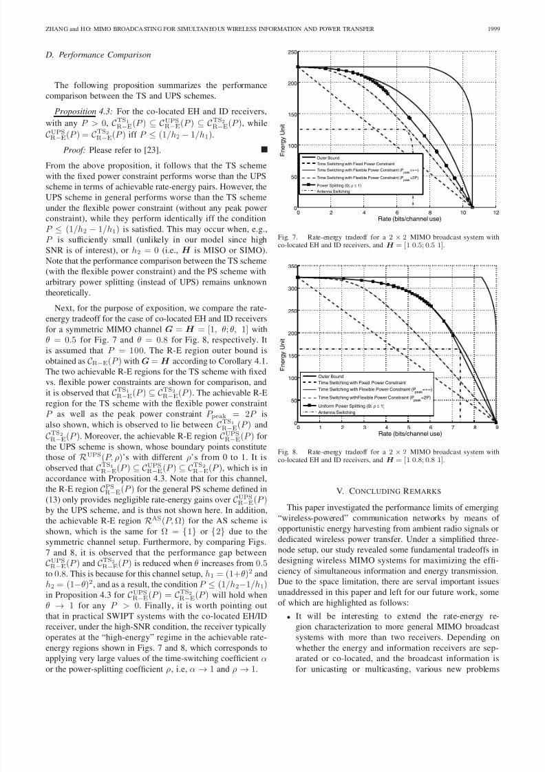
Next, for the purpose of exposition, we compare the rate-
energy tradeoff for the case of co-located EH and ID receivers
for a symmetric MIMO channel G = H = [1, θ; θ, 1] withθ = 0.5 for Fig. 7 and θ = 0.8 for Fig. 8, respectively. It
is assumed that P = 100. The R-E region outer bound is
obtained as CR−E(P ) withG = H according to Corollary 4.1.
The two achievable R-E regions for the TS scheme with fixed
vs. flexible power constraints are shown for comparison, and
it is observed that CTS1R−E(P ) ⊆ CTS2R−E(P ). The achievable R-E
region for the TS scheme with the flexible power constraintP as well as the peak power constraint P peak = 2P is
also shown, which is observed to lie between CTS1R−E(P ) and
CTS2R−E(P ). Moreover, the achievable R-E region CUPSR−E(P ) for
the UPS scheme is shown, whose boundary points constitutethose of RUPS(P, ρ)’s with different ρ’s from 0 to 1. It is
observed that CTS1R−E(P ) ⊆ CUPSR−E(P ) ⊆ CTS2R−E(P ), which is in
accordance with Proposition 4.3. Note that for this channel,
the R-E region CPSR−E(P ) for the general PS scheme defined in
(13) only provides negligible rate-energy gains over CUPSR−E(P )by the UPS scheme, and is thus not shown here. In addition,
the achievable R-E region RAS(P, Ω) for the AS scheme is
shown, which is the same for Ω =
1
or
2
due to the
symmetric channel setup. Furthermore, by comparing Figs.7 and 8, it is observed that the performance gap between
CUPSR−E(P ) and CTS2R−E(P ) is reduced when θ increases from 0.5to 0.8. This is because for this channel setup, h1 = (1+θ)2 andh2 = (1−θ)2, and as a result, the condition P ≤ (1/h2−1/h1)in Proposition 4.3 for CUPSR−E(P ) = CTS2R−E(P ) will hold whenθ → 1 for any P > 0. Finally, it is worth pointing out
that in practical SWIPT systems with the co-located EH/ID
receiver, under the high-SNR condition, the receiver typically
operates at the “high-energy” regime in the achievable rate-
energy regions shown in Figs. 7 and 8, which corresponds toapplying very large values of the time-switching coefficient αor the power-splitting coefficient ρ, i.e, α
→1 and ρ
→1.
0 2 4 6 8 10 120
50
100
150
200
250
Rate (bits/channel use)
E n e r g y U n i t
Outer Bound
Time Switching with Fixed Power Constraint
Time Switching with Flexible Power Constraint (Ppeak
=+∞)
Time Switching with Flexible Power Constraint (Ppeak
=2P)
Power Splitting (0≤ ρ ≤ 1)
Antenna Switching
Fig. 7. Rate-energy tradeoff for a 2 × 2 MIMO broadcast system withco-located EH and ID receivers, and H = [1 0.5; 0.5 1].
0 1 2 3 4 5 6 7 8 90
50
100
150
200
250
300
350
Rate (bits/channel use)
E n e r g y U n i t
Outer Bound
Time Switching with Fixed Power Constraint
Time Switching with Flexible Power Constraint (Ppeak
=+∞)
Time Switching withFlexible Power Constraint (Ppeak
=2P)
Uniform Power Splitting (0≤ ρ ≤ 1)Antenna Switching
Fig. 8. Rate-energy tradeoff for a 2 × 2 MIMO broadcast system withco-located EH and ID receivers, and H = [1 0.8; 0.8 1].
V. CONCLUDING REMARKS
This paper investigated the performance limits of emerging
“wireless-powered” communication networks by means of
opportunistic energy harvesting from ambient radio signals or
dedicated wireless power transfer. Under a simplified three-node setup, our study revealed some fundamental tradeoffs in
designing wireless MIMO systems for maximizing the effi-
ciency of simultaneous information and energy transmission.Due to the space limitation, there are serval important issues
unaddressed in this paper and left for our future work, some
of which are highlighted as follows:
• It will be interesting to extend the rate-energy re-
gion characterization to more general MIMO broadcast
systems with more than two receivers. Depending on
whether the energy and information receivers are sep-arated or co-located, and the broadcast information is
for unicasting or multicasting, various new problems

8/13/2019 MIMO Broadcasting for Simultaneous Wireless Information and Power Transfer
http://slidepdf.com/reader/full/mimo-broadcasting-for-simultaneous-wireless-information-and-power-transfer 12/13
2000 IEEE TRANSACTIONS ON WIRELESS COMMUNICATIONS, VOL. 12, NO. 5, MAY 2013
can be formulated for which the optimal solutions are
challenging to obtain.
• For the case of co-located energy and information re-
ceivers, this paper shows a performance bound that
in general cannot be achieved by practical receivers.
Although this paper has shed some light on practicalhardware designs to approach this limit (e.g., by the
power splitting scheme), further research endeavor is stillrequired to further reduce or close this gap, even for the
SISO AWGN channel.
• In this paper, to simplify the analysis, it is assumed that
the energy conversion efficiency at the energy receiver
is independent of the instantaneous amplitude of the
received radio signal, which is in general not true forpractical RF energy harvesting circuits [21]. Thus, how
to design the broadcast signal waveform, namely energy
modulation, to maximize the efficiency of energy transfer
to multiple receivers under practical energy conversion
constraints is an open problem of high practical interests.• Unlike the traditional view that the receiver noise and/or
co-channel interference degrade the communication link reliability [22], they are however beneficial from the
viewpoint of RF energy harvesting. Thus, there exist non-
trivial tradeoffs in allocating communication resources to
optimize the network interference levels for achieving
maximal information vs. energy transfer. More studies
to reveal such tradeoffs are worth pursuing.
APPENDIX A
PROOF OF THEOREM 3.1
The Lagrangian of (P3) can be written as
L(S , λ , µ) = log I + HSH H + λtrGSGH − Q
− µ (tr(S ) − P ) . (14)
Then, the Lagrange dual function of (P3) is defined as
g(λ, µ) = maxS 0 L(S , λ , µ), and the dual problem of (P3),
denoted as (P3-D), is defined as minλ≥0,µ≥0 g(λ, µ). Since(P3) can be solved equivalently by solving (P3-D), in the
following, we first maximize the Lagrangian to obtain the dual
function with fixed λ ≥ 0 and µ ≥ 0, and then find the optimal
dual solutions λ∗ and µ∗ to minimize the dual function. The
transmit covariance S ∗ that maximizes the Lagrangian to
obtain g (λ∗, µ∗) is thus the optimal primal solution of (P3).
Consider first the problem of maximizing the Lagrangian
over S with fixed λ and µ. By discarding the constantterms associated with λ and µ in (14), this problem can be
equivalently rewritten as
maxS 0
logI + HSH H
− tr
µI − λGH G
S
. (15)
Recall that g1 is the largest eigenvalue of the matrix GH G.
We then have the following lemma.
Lemma A.1: For the problem in (15) to have a bounded
optimal value, µ > λg1 must hold.
Proof: We prove this lemma by contradiction. Supposethat µ ≤ λg1. Then, let S = β v1vH 1 with β being any
positive constant. Substituting S into (15) yields log(1 +
TABLE IALGORITHM FOR SOLVING PROBLEM (P3).
Initialize λ ≥ 0, µ ≥ 0, µ > λg1Repeat
Compute S using (17) with the given λ and µCompute the subgradient of g (λ, µ)Update λ and µ using the ellipsoid method subject to µ > λg1 ≥ 0
Until λ and µ converge to the prescribed accuracySet S ∗ = S
β Hv12) + β (λg1 − µ). Since H and G are either inde-
pendent (in the case of separated receivers) or identical (inthe case of co-located receivers), it is valid to assume that
Hv12 > 0 and thus the value of the above function or
the optimal value of Problem (15) becomes unbounded whenβ → ∞. Thus, the presumption that µ ≤ λg1 cannot be true,
which completes the proof.
Since Problem (P3) should have a bounded optimal value,
it follows from the above lemma that the optimal primal anddual solutions of (P3) are obtained when µ > λg1. Let A =µI
−λGH G. It then follows that A
0 with µ > λg1, and
thus A−1 exists. The problem in (15) is then rewritten as
maxS 0
logI + HSH H
− tr (AS ) . (16)
Let the (reduced) SVD of the matrix HA−1/2 be given by
HA−1/2 = U Γ1/2V H
, where U ∈ CM ×T 2 , V ∈ CM ×T 2 ,
Γ = diag(h1, . . . , hT 2), with h1 ≥ h2 ≥ . . . ≥ hT 2 ≥ 0. It
has been shown in [17] under the CR setup that the optimal
solution to Problem (16) with arbitrary A 0 has the
following form:
S = A−1/2V ΛV H A−1/2 (17)
where Λ = diag(˜ p1, . . . , ˜ pT 2), with ˜ pi = (1 − 1/hi)+, i =1, . . . , T 2.
Next, we address how to solve the dual problem (P3-D)
by minimizing the dual function g(λ, µ) subject to λ ≥ 0,µ ≥ 0, and the new constraint µ > λg1. This can be done
by applying the subgradient-based method, e.g., the ellipsoid
method [20], for which it can be shown (the proof is omittedfor brevity) that the subgradient of g(λ, µ) at point [λ, µ] isgiven by [tr(GS GH ) − Q, P − tr(S )], where S is given
in (17), which is the optimal solution of Problem (15) for a
given pair of λ and µ. When the optimal dual solutions λ∗
and µ∗ are obtained by the ellipsoid method, the corresponding
optimal solution S for Problem (15) converges to the primal
optimal solution to Problem (P3), denoted by S ∗. The aboveprocedures for solving (P3) are summarized in Table I. Theproof of Theorem 3.1 is thus completed.
APPENDIX B
PROOF OF PROPOSITION 4 .2
Since H ≡ h [h1, . . . , hN ]T , for any set of ρi’swith 0 ≤ ρi ≤ 1, the harvested power is equal to Q =P N
i=1 ρi|hi|2. Clearly, 0 ≤ Q ≤ h||2P . The equivalent
SIMO channel for decoding information then becomes h [√
1 − ρ1h1, . . . ,√
1 − ρN hN ]T . Since for the SIMO channel,
the transmit covariance matrix degrades to a scalar equal to

8/13/2019 MIMO Broadcasting for Simultaneous Wireless Information and Power Transfer
http://slidepdf.com/reader/full/mimo-broadcasting-for-simultaneous-wireless-information-and-power-transfer 13/13
ZHANG and HO: MIMO BROADCASTING FOR SIMULTANEOUS WIRELESS INFORMATION AND POWER TRANSFER 2001
P , the maximum achievable rate is given by (via applying the
MRC beamforming at ID receiver):
R =log
1 + h2P
(18)
=log
1 +
N i=1
(1 − ρi)|hi|2P
(19)
=log
1 +
N i=1
|hi|2P −N i=1
ρi|hi|2P
(20)
=log
1 + h2P − Q
. (21)
We thus have CPSR−E(P ) = (R, Q) : R ≤ log(1 + (h2P −Q)), 0 ≤ Q ≤ h2P . Furthermore, since the above proof
is valid for any ρi’s and changing ρ from 0 to 1 yields the
value of Q = P ρN
i=1 |hi|2 from 0 to h||2P , it thus follows
that CUPSR−E(P ) = (R, Q) : R ≤ log(1 + (h2P − Q)), 0 ≤Q ≤ h2P , which is the same as CPSR−E(P ). The proof of
Proposition 4.2 is thus completed.
REFERENCES
[1] L. R. Varshney, “Transporting information and energy simultaneously,”in Proc. 2008 IEEE Int. Symp. Inf. Theory , pp. 1612–1616.
[2] P. Grover and A. Sahai, “Shannon meets Tesla: wireless informationand power transfer,” in Proc. 2010 IEEE Int. Symp. Inf. Theory, pp.2363–2367.
[3] R. Want, “Enabling ubiquitous sensing with RFID,” IEEE Computer ,vol. 37, pp. 84–86, Apr. 2004.
[4] G. Landis, M. Stavnes, S. Oleson, and J. Bozek, “Space transfer withground-based laser/electric propulsion,” NASA Technical Memorandum,TM-106060, 1992.
[5] F. Zhang et al., “Wireless energy transfer platform for medical sensorsand implantable devices,” in Proc. 2009 IEEE EMBS 31st Annual Int.
Conf., pp. 1045–1048.[6] I. E. Telatar, “Capacity of multi-antenna Gaussian channels,” Eur. Trans.
Telecommun., vol. 10, no. 6, pp. 585–595, Nov. 1999.[7] G. Carie and S. Shamai, “On the achievable throughput of a multi-
antenna Gaussian broadcast channel,” IEEE Trans. Inf. Theory, vol. 49,
no. 7, pp. 1691–1706, July 2003.[8] P. Viswanath and D. Tse, “Sum capacity of the vector Gaussian broad-
cast channel and uplink-downlink duality,” IEEE Trans. Inf. Theory, vol.49, no. 8, pp. 1912–1921, Aug. 2003.
[9] S. Vishwanath, N. Jindal, and A. Goldsmith, “Duality, achievable rates,and sum-rate capacity of Gaussian MIMO broadcast channels,” IEEE
Trans. Inf. Theory, vol. 49, no. 10, pp. 2658–2668, Oct. 2003.[10] W. Yu and J. M. Cioffi, “Sum capacity of Gaussian vector broadcast
channels,” IEEE Trans. Inf. Theory, vol. 50, no. 9, pp. 1875–1892, Sep.2004.
[11] N. D. Sidiropoulos, T. N. Davidson, and Z.-Q. Luo, “Transmit beam-forming for physical-layer multicasting,” IEEE Trans. Signal Process.,vol. 54, pp. 2239–2251, June 2006.
[12] N. Jindal and Z.-Q. Luo, “Capacity limits of multiple antenna multicast,”in Proc. 2006 IEEE Int. Symposium Inf. Theory, pp. 1841–1845.
[13] T. Cover and J. Thomas, Elements of Information Theory. Wiley, 1991.[14] L. R. Varshney, “Unreliable and resource-constrained decoding,” Ph.D.
Thesis, EECS Department, MIT, June 2010.
[15] M. Gastpar, “On capacity under receive and spatial spectrum-sharingconstraints,” IEEE Trans. Inf. Theory, vol. 53, no. 2, pp. 471–487, Feb.2007.
[16] R. Zhang and Y. C. Liang, “Exploiting multi-antennas for opportunisticspectrum sharing in cognitive radio networks,” IEEE J. Sel. TopicsSignal Process., vol. 2, no. 1, pp. 88–102, Feb. 2008.
[17] R. Zhang, Y. C. Liang, and S. Cui, “Dynamic resource allocation incognitive radio networks,” IEEE Signal Process. Mag., vol. 27, no. 3,pp. 102–114, May 2010.
[18] S. Boyd and L. Vandenberghe, Convex Optimization. Cambridge Uni-
versity Press, 2004.[19] J. Proakis, Digital Communication. McGraw-Hill Science Press, 2000.[20] S. Boyd, “Convex optimization II,” Stanford University. Available:
http://www.stanford.edu/class/ee364b/lectures.html
[21] T. Le, K. Mayaram, and T. Fiez, “Efficient far-field radio frequencyenergy harvesting for passively powered sensor networks,” IEEE J.Solid-State Circuits, vol. 43, no. 5, pp. 1287–1302, May 2008.
[22] V. R. Cadambe and S. A. Jafar, “Interference alignment and the degreesof freedom for the K user interference channel,” IEEE Trans. Inf. Theory,vol. 54, no. 8, pp. 3425–3441, Aug. 2008.
[23] R. Zhang and C. K. Ho, “MIMO broadcasting for simultaneous wirelessinformation and power transfer.” Available: arXiv:1105.4999.
Rui Zhang (S’00–M’07) received the B.Eng. (First-Class Hons.) and M.Eng. degrees from the Na-tional University of Singapore in 2000 and 2001,
respectively, and the Ph.D. degree from the Stan-ford University, Stanford, CA USA, in 2007, all inelectrical engineering. Since 2007, he has workedwith the Institute for Infocomm Research, A*STAR,Singapore, where he is now a Senior Research Sci-entist. Since 2010, he has joined the Department of Electrical and Computer Engineering of the NationalUniversity of Singapore as an Assistant Professor.
His current research interests include multiuser MIMO, cognitive radio,cooperative communication, energy efficient and energy harvesting wirelesscommunication, wireless information and power transfer, smart grid, andoptimization theory. He was the co-recipient of the Best Paper Award from theIEEE PIMRC in 2005. He was the recipient of the 6th IEEE ComSoc Asia-Pacific Best Young Researcher Award in 2010, and the Young InvestigatorAward of the National University of Singapore in 2011. He is now an electedmember of IEEE Signal Processing Society SPCOM and SAM TechnicalCommittees, and an editor for the IEEE T RANSACTIONS ON WIRELESS
COMMUNICATIONS.
Chin Keong Ho received the B. Eng. (First-ClassHons., Minor in Business Admin.), and M. Engdegrees from the Department of Electrical Engineer-ing, National University of Singapore in 1999 and2001, respectively. He obtained his Ph.D. degree in2009 at the Eindhoven University of Technology,The Netherlands, where he concurrently conductedresearch work in Philips Research. Since August2000, he has been with Institute for Infocomm Re-search (I2R), A*STAR, Singapore. He is currentlyActing Lab Head of Energy-Aware Communications
Lab, Department of Modulation and Coding, in I2R. His research inter-est includes green wireless communications with focus on energy-efficientsolutions and with energy harvesting constraints; cooperative and adaptivewireless communications; and implementation aspects of multi-carrier and
multi-antenna communications.