THE APPLICATION OF TREND ANALYSIS

TO AGRICULTURAL J:!'IELD TRIALS

by

Herbert J. Kirk

Institute of StatisticsMimeograph Series No. 1093Raleigh, N.C. November 1976

v

TABLE OF CONTENTS

Page

1. INTRODUCTION. . . . 1

2. REVIEW OF LITERATURE 10

2.1.2.2.

The Occurrence of Fertility GradientsCompensating for Fertility Gradients by use of

Trend Analysis

10

12

3 . PROCEDURE TREND 17

1718181925

26

2929

28

31

32333334

Multiple3.2.6.1.3.2.6.2.

of AnalysisMathematical ModelSelection of a Response Surface ModelAnalysis of Variance . . . . . . . •Solving the Normal Equation Using a

Sweep Operator • . . . . . . • . . •Computation of Treatment Estimates and Sum

of Squares in Analysis of Variance .3.2.5.1. General Mean and Total Sum of

Squares . • • . • • . . . •3.2.5.2. Treatment Means and Sum of Squares.3.2.5.3. Coefficients and Sum of Squares for

the Response Surface Model3.2.5.4. Adjusted Treatment Means and Sum of

Squares . . • . . • . . .Comparisons of Adjusted MeansStudent's t~test ....Bayesian K-ratio t-test

IntroductionMethod3.2.1.3.2.2.3.2.3.3.2.4.

3.2.5.

3.2.6.

3.1.3.2.

4. SIMULATED DATA EXPERIMENT 35

4.1.4.2.4.3.4.4.

Introduction . • • • .Materials and MethodsResultsDiscussion . . • . • . .

35353750

5. POTATO CULTIVAR FIELD EXPERIMENT 51

5.1.5.2.5.3.5.4.

Introduction . . . . .Materials and MethodsResultsDiscussion . . . . . .

51525672

TABLE OF CONTENTS (continued)

6. SUMMARY AND CONCLUSIONS

vi

Page

75

6.1.6.2.6.3.

Sunnnary .....Conclusions and ReconnnendationsSuggestions for Future Investigation6.3.1. Size and Shape of Plots6.3.2. Tests for Normality and Autocorrelation of

Residuals . . . . . . . . . • . • .6.3.3. Determination of Bias in Estimation ...•6.3.4. Error Rates ...•.

75767777

777878

7. LIST OF REFERENCES

8. APPENDICES. . ••

79

82

8.1.8.2.

8.3.

8.4.

8.5.

8.6.

8.7.

8.8.

8.9.

8.10.

8.11.

8.12.

A Write-up of Procedure TREND Along With an ExampleComparison of Known with Estimated Treatment Effects

Obtained From Unadjusted and Adjusted TreatmentMeans Using the Simulated Data • . . . • • • . • •

Estimates of Error Variance Using Standard DesignAnalysis and Trend Analysis for Different YieldResponses . • • • " . . • 0 • • e • • • • • • •

Percent Gain in Relative Efficiency Due to Design orTrend Analysis Using Estimates of Error Variance forDifferent Yield Responses . • . • • • • . • • . • • •

Ranked Cultivar Means (Before and After Adjusting forTrend) Using Yield of Size A Tubers from Field E-3 • •

Ranked Cultivar Means (Before and After Adjusting forTrend) Using Yield of Size A Tubers from Field L-2 • .

Ranked Cultivar Means (Before and After Adjusting forTrend) Using Yield of Size B Tubers from Field E-3 .

Ranked Cultivar Means (Before and After Adjusting forTrend) Using Yield of Size B Tubers from Field L-2 • •

Ranked Cultivar Means (Before and After Adjusting forTrend) Using Yield of Culls from Field E-3 . • • . • .

Ranked Cultivar Means (Before and After Adjusting forTrend) Using Yield of Culls from Field L-2 • . • . •

Ranked Cultivar Means (Before and After Adjusting forTrend) Using Marketable Yield from Field E~3 • • . . •

Ranked Cultivar Means (Before and After Adjusting forTrend) Using Marketable Yield from Field L-2 • • . . .

83

97

98

99

100

101

102

103

104

105

106

107

1. INTRODUCTION

Experimental results from agricultural field trials are obscured by

the effect of two types of disturbing factors: (1) the effect of factors

displaying an unknown, systematic variation and (2) the effect of random

factors. The systematic variation is directly related to the position of

the plot in the field and is referred to as a fertility gradient or simply,

"trend." The variation may be attributed to many factors such as

weediness, water drainage, directions of winds, as well as fertility of

the soil. The random factor is called pure error and is caused by

measurement errors, genetic variation, plus a great number of small

additive effects. The total experimental error is composed of variations

originating from these two sources.

The magnitude of experimental error is a question of major importance

in agricultural field research because its proper recognition determines

the degree of confidence which may be attached to the results obtained in

field work. Not only does this fertility gradient inflate the experimental

error but it also causes lack of independence among the quantities usually

assumed to be independent in the data analysis. Neighbouring plots tend

to be positively correlated. This condition impairs the entire theoretical

basis of the standard analyses, and in particular, is liable to invalidate

the estimates of error and tests of significance.

A fundamental problem in most agricultural field trials is, thereforei

to eliminate as much as possible the effect of the fertility gradient from

experimental error. Two methods are available for this purpose: (1) the

design of the experiment, i.~., selection of the plots and the allocation

of the treatments to them, and (2) the statistical technique used in the

analysis of the results.

2

Many standard textbooks in experimental design such as Snedecor and

Cochran (1967), Cochran and Cox (1957), Federer (1955), and others,

state that if the field is more or less homogeneous, then the appropriate

model is

(1.1)

where

Y•• = observation on unit j of the .th treatment,11.J

IJ. .- general mean,

= effect of the .th treatment, and'1". 1.1.

d f h .th. h .thran om error 0 t e J un:Lt on t e :Ltreatment

and assumed that € •• rv NID (0 , dd) .1.J

Equation (1.1) is the model for the completely randomized design.

Treatments are assigned to the experimental units entirely at random

and with no restrictions (except that of equal numbers of plots per

treatment, usually).

If it is possible to group the experimental units by some common

feature which influences yield, i.e., to stratify the field on the basis

of the fertility gradients into "blocks" which are as internally

homogeneous as possible, then the mathematical model used is

(1. 2)

where

Y•• = observation in the j th block for the .th treatment,1.1.J

IJ. = general mean,

effect of the .th'1". = 1. treatment,

1.

I3 j = effect common to all units i.n the jth block, and

E ••1.J

= random error associated with the i th treatment in the

jth block and assumed that

3

Equation (1.2) is the model for the randomized complete block design.

Treatments are randomly assigned to the experimental units with the

restriction that each treatment occurs once (or equally often) in each

block..

If it is possible to find another system of grouping which

influences yield, then the experimental units may be grouped according

to two classifications and the resulting mathematical model is

(1.3)

where

Yij(k) b . f h' th . h . tho servat1.on 'or t e 1. treatment, 1.n t e J group

according to the first classification and in the kth

group according to the second classification,

IJ. = general mean,

effec.t of the .th'T. = 1. treatment,

J.

I3 j= effect to all units in the .thcommon J group

according to the first classification,

thYk effect common to all units in the k group

Eij(k)

according to the second classification, and

random error associated with the ith

treatment

occuring in the jth group first classification

thand k group second classification and assumed

Eij(k) '" NID (0 , rf) .

Equation (1.3) is the model for t.he J~atin square design. Treatments

4

are randomly assigned to the experimental units with the restrictions

that each treatment occurs once and only once for each group of the

first and of the second classification.

The most commonly used designs in agricultural field trials are

the randomized complete block and the Latin square. These designs are

based upon a combinati.on of systematic and random arrangements of the

treatments. As a result, part of the fertility gradient is eliminated

from the experimental error by means of the systematic structure of

the experiment and part by the analysis of variance. The remaining

variation due to fertility gradients is included in the experimental

error, but characteristically is treated as a random factor. Here, the

analysis of variance is taken, in its usual sense, as the application

of the method of least squares under the assumption that the fertility

gradient may be estimated or described by a step-function, in which,

for example, in the randomized block experiment, takes on a new value

for every block, but is constant within a block. This method is often

unsatisfactory for a large number of treatments (i.&., large blocks)

because the plots within a block are not approximately of the same

level of fertility. If a Latin square design is used, the gradients

are estimated by a two dimensional step function which cannot account

for row by column interactions. Another limitation of this design is

that prior information on the fertility gradient is required before

the treatments are assigned to the experimental units. In many

experiments this information is not available when the plot plan is

developed, resultin.g in a possibly inefficient design inadequate for

eliminating the trend variation from experimental error. Even when

5

the proper design is used, during the duration of the experiment,

environmental conditions, pests, or other factors may cause a systematic

variation in the experimental response.

Another technique for eliminating systematic variability from

experimental error is by trend analysis 0 In trend analysis a grid

is superimposed on the field by identifying rows and tiers which

define the location of each plot. The systematic variability is

removed by fitting a polynomial regression equation to the fertility

gradient using rows and tiers as the independent variables in the

polynomial function. The approximation of any continuous function

by a power series is a result from the calculus usually called

"Taylor's Theorem." When a polynomial regression equation is used

as an approximation, the resulting function has come to be known as

a "response surface" model. A general form of the mathematical model

used is

p ~ q p q ~

Y 0 ( 0 k) = I-L + T 0 + I: 13 n R 0 + I: 13 ~k+ I: I: 13 n_RJo ~k+ e: 1.' ( 0 k) ,1. J 1. ~l ",,0 J m=l om ~l m=l Mil J

where

(1.4)

Yi(jk) = observation for the .thlocated on1. tre atment,

the .th and kth

tier,J row

I-L = general mean,

'T. =: effect of the .th treatment,1.1.

P~ . th

I: ,13~ R. = polynomial regression effect of the J row~=l

o J

coordinate (p = number rows ~ 1),q

kth

m~ll3om~ = polynomial regression effect of the tier

coordinate (q = number tiers - 1) ,

between the jth row and kth tier coordinate, and

p q i-t t ShnR.~ = polynomial regression effect of the interaction

i-=l m=l J

6

€i(jk) = random error associated with the response, assumed

€i(jk) ,..., NID (0 ,,sa).

Trend analysis has an advantage over standard design analysis in

that the mathematical model is not fixed by the experimental design.

A separate response surface model is developed for each analysis, and

the model contains only terms that are significantly related to the

fertility gradient. Trend analysis may be regarded as a method which

optimizes the number of degrees of freedom available for estimating

experimental error. A major advantage of trend analysis is that its

efficiency will be greater than or equal to that of the standard

design analysis. This point can be illustrated by considering the

four possible forms of a fertility gradient.

1) Suppose that a fertility gradient did not exist in the

field. The experimental units would be homogeneous, and

the fitting of a polynomial regression equation would be

irrelevant. The mathematical model for the trend analysis

would be

(1.5)

which is equivalent to the model appropriate for a

completely random design.

2) Suppose a one dimensional fertility gradient existed in

the field and ran perpendicular to the rows. Only row

terms would be relevant in fitting of a polynomial

7

regression equation. The mathemati.cal model for the trend

analysis would be

(1.6)

and, if all p degrees of freedom are required to explain the

fertility gradient, this model is equivalent to that appro-

priate for a randomized complete block design.

3) Suppose a simple two dimensional fertility gradient existed

in the fi.eld and ran parallel to both rows and tiers. Both

row and tier effects would be relevant in fitting a polynomial

regression equation. The mathematical model for the trend

analysis would be

P t q ....InY. ( .k) = j.L + 'T • + I: Sn R. + I: S T.k + e . ( .' k) ,~ J. ~ t=l NO J m=l om ~ J.

(1. 7)

and, if all p and q degrees of freedom are required to explain

the fertility gradient, this model is equivalent to that of a

Latin square design.

4) Suppose a complex two dimensional fertility gradient existed

forming a surface containing peaks, valleys, and ridges. Row,

tier, and row by tier interaction effects would be relevant in

fitting a polynomial regression equation to this type of

surface. Under these conditions, trend analysis should be

more efficient than any standard design model, since no

design exists which can account for the row by tier inter-

action.

This study was conducted to determine how much could be gained in

efficiency by describing the systematic variation in a standard design

8

experiment by a properly chosen response surface model. The degree of

success depends partly on the nature of the fertility gradient itself,

the gain being largest in cases wi.th a large amount of systematic

variability. The additional computational labor required for a

fi.tted response surface of the fertility gradient instead of a step-

function would be conSiderable, and a computer program is required

for routine applications. If it can be shown that it is possible to

eliminate nearly all the systematic variability by a trend analysis,

then it follows that the arrangement of the treatments within the

blocks (or within rows and columns) is not necessarily critical to

the analysis of the results.

The objectives of this study are as follows:

1) To develop a FORTRAN computer program linked with the

Statistical Analysis System (SAS)l which would automate

the difficult computations required for trend analysis.

(a) The computer program would contain the decision making

capability to develop an adequate response surface model

explaining the systematic variability in the experiment.

(b) Based upon the selected response surface model, the

program would compute the appropriate analysis of

variance, adjusted treatment means, and tests of

signifi.cance.

lSAS embodies an integrated approach to the editing and statisticalanalysis of data and was developed by Mr. A. J. Barr and Dr. J. H.Goodnight (1972).

9

2) To simulate data for the purpose of comparing known variance

and treatment parameters with their respective estimates from

the trend analysis procedure.

(a) To determine if the computer program could develop an

adequate response surface model for eliminating systematic

variation from experimental error,

(b) To determine if adjusting the treatment means using the

selected response surface model results in an improved

estimate of the treatment effects,

3) To conduct an actual field experiment for the purpose of

determining how much could be gained in efficiency by

describing the systematic variation in a standard design

experiment by an adequately chosen response surface model.

(a) To determine if an adequate response surface model

could be fitted to the fertility gradient of an

agricultural field trial.

(b) To determine if randomization of the treatments has any

effect on the results obtained from trend analysis when

applied to agricultural field trials,

(c) To evaluate the overall feasibility of using trend

analysis for analyzing agricultural field trials,

10

2. REVIEW OF LITERATURE

2.1. The Occurrence of Fertility Gradients

It has been common knowledge that in agricultural field trials the

characterization of soil variation is necessary for proper interpretation

of experimental results. There are other sources of variation confounded

with the soil variation such as the spread of pests and diseases, winds,

water drainage, irrigation, and farm machinery practices, to name a few.

The interactions among these factors may be considered as causing a

systematic pattern or fertility gradients in the field.

Since the beginning of the twentieth century, uniformity trials

were used to study variability in agricultural fi.e1ds. These trials

are conducted on a field that is treated as uniformly as possible. The

responses of small units are measured and recorded separa1:ely . for each

unit along with its geographic location.

A great number of uniformity trials have been conducted allover

the world for a wide range of crops. Cochran (1937) published a

Catalogue of Uniformity Trials listing most of the uniformity trials

performed before 1937. Pearce (1953) cataloged uniformity trials of

fruit trees and other perennial plants. A partial catalogue of

uniformity trials is published in Salmon (1955).

From early studies of uniformity trials, the inference was made

that the plots have certain tendencies or trends in their productivity

because of the positive correlation among neighboring plots.' Later,

the idea developed that plot yields may be composed of two parts:

(1) a part related to the geographic location of the plot (trend or

fertility gradient) and (2) a part not related to the plot location

11

(random error). These principal ideas are discussed i.n several

important studies.

Richey (1926) was one of the first to point out that field plots

have certain trends in productivity. He indicated that productivity

of the soil does not change abruptly but more or less gradually, so

that adjacent plots are more nearly alike than plots that are

farther apart. Stephens and Vinal1 (1928) studied field experiments

with sorghum in which they presented a figure showing high, medium

and low yielding areas with a systematic pattern. The graph

suggested (the existenace of) islands of variation later proposed

by Hoyle and Baker (1961). Immer and Ralei.gh (1933), working with

sugar beets, found that yield was influenced by the systematic nature

of soil heterogeneity.

Wellman et a1. (1948) suggested that the variation in plot

yields from uniformity trials can be divided into: (1) uncontrolled,

unorganized variation (the true error of an experiment) and (2) an

organized variation attributable to the geographic position of each

plot within the experiment. They also suggested that the latter

variation can be caused by such factors as weediness, air drainage

and direction of prevailing winds, as well as by soil fertility and

moisture. It would be improper, in their view, to call it soil

variation, and they suggested the term "geographic variation,"

A closely related concept to geographic variation is the Ilisland

of variation" as defined by Hoyle and Baker (1961). They defined an

island of variation as a group of values within which a con~on level

of productivity potential exists regardless of any superimposed

12

treatments. They showed that areas of similar productivity occur often

and can be mapped as irregular areas with a connected geographic

boundary. Ferguson (1962) indicated that environmental conditions

generally change gradually from place to place in the field, causing

adjacent plots to be correlated.

The findings of uniformity trials were best summarized by

LeClerg et a1. (1962). They suggested that uniformity trials have

established the fact that soil fertility cannot be regarded as

randomly distributed. To the extent that soil fertility is systematic,

contiguous plots are likely to be more similar than those farther

apart.

2.2. Compensating for Fertility Gradients

by use of Trend Analysis

It seems established from the previous work cited that fertility

gradients do exist in agricultural field trials. Yates (1939) pointed

out that for its correct application, the method of least squares

requires that any components of variation which are not eliminated

by the experimental design shall be normally and independently

distributed. It is evident that the yields of agricultural field

plots (even after allowing for the effects of local control, such as

blocks) are not independently distributed, and, in particular, this

condition is liable to vitiate completely the estimates of error and

tests of significance. Logically, given that plot yields are

correlated, a continuous function of some form may be fitted to the

systematic variation in the experimental units. It follows that such

13

a trend analysis may be applied in which the fitted function eliminates

serious trend effects from the experimental error,

Neyman et a1. (1935) was one of the first investigators to suggest using

some form of a functional model to explain systematic soil variation,

He proposed using a polynomial regression equation for describing

the fertility variation in experiments, where the treatments were

arranged in the same order in every block and where the blocks were

placed in succession,

Van Uven (1935) considered the adjustment of yields in field

experiments according to the condition of the soil. He developed

formulae to correct yield assuming a linear or quadratic trends in

soil fertility. The adjustments were based on fertility maps which

showed the residuals for each plot obtained by subtracting from each

plot yield the mean of the treatment applied to that plot. He

suggested that the type of correction should be determined after

looking at the fertility map. For two different tr~atments he

suggested the fitting of different equations of fertility, and then

comparing yields at equal levels of fertility,

In a discussion paper, Jeffreys (1939) suggested that standard

design models were inadequate to compensate for trend effects. The

Latin square, for example, can account for variation in two directions

(rows and columns) but in no way can it deal with a term such as row

by column interaction. Jeffreys proposed using a full polynomial

model, including all high order interactions to represent the fertility

gradient. He went on to say that the analysis would be prohibitively

difficult.

14

Hald (1948) developed a technique using orthogonal polynomials for

the purpose of removing systematic variation from experimental error. He

found that in about 20 actual field experiments the method seemed to work

satisfactorily. The fertility gradient was described by polynomials of

up to the fifth degree and the residual variation therefrom seemed to be

random.

In 1950 at the International Biometric Conferences, R. A, Fisher

pointed out that the method of fitting polynomials in one or two

dimensions was not as new or unexplored as Hald suggested. For many

years Fisher himself frequently tested what could be done wi.th field

trials by these methods. He concluded that the principal difficulty

encountered, once the labor of such analysis had been overcome, was

that fitted polynomials in two dimensions might easily absorb 20 or 30

degrees of freedom without removing a corresponding proportion of the

residual sum of squares.

Upon Fisher's criticisms of the method of fitting polynomials,

little research on this method was reported in the literature until

1954. Federer and Schlottfeldt (1954) illustrated the use of covariance

to control gradients in an experiment as a substitute for deliberate

stratification in the design. They discussed measurements of the

heights of tobacco plants in an experiment with seven treatments

arranged in eight randomized blocks. A fertility gradient within

the blocks was suspected, and they calculated a quadratic covariance

analysis on a measure of distance in this direction. They concluded

that the use of covariance to control the gradient across the treatment

plots approximately doubled the amount of information.

15

Federer and Schlottfe1dt (1954) also pointed out that covariance

analysis will usually be more effective than using rough groupings of

size for the rows or c.olumns of a 1.atin square. In addi tioD, the

utilization of covariance does not require as many degrees of freedom

to be allocated as does stratification into rows or columns.

The same tobacco experiment data were further analyzed by Outhwaite

and Rutherford (1955), including as covariates orthogonal polynomials

up to the sixth degree. Tests of significance strongly indicated that

a covariance adjustment ought to include up to the fifth degree

component. They also pointed out that the variance of the adjusted

means should be corrected to allow for the sampling errors of the

coefficients and gave a general formula for the average value of the

corrections. The corrected variances were used to calculate the

gains in information from the covariance analysis. They concluded

that the full covariance adjustment was less efficient than a 7 X7

Latin square with the same variance per plot. The advantage gained

by having an extra replication was lost by the extreme non-orthogonality.

The writer believes that the reason these and other researchers

were unsuccessful in adjusting for trend effects was that they were

using an inadequate functional model. During the time of their

research, neither computers nor sufficient software were available to

allow the researcher an opportunity to investigate alternative models.

The feasibility of using trend analysis, given an appropriate response

surface model, was indicated by Mendez (1970). Using uniformity field

trials with superimposed treatment effects, he compared six alternatives

to blocking for the desi.gn and analysis of field experiments. He

16

concluded that if the number of treatments is large, say five or more,

then trend analysis should be considered. After investigating many

uniformity trials he also concluded that no single degree polynomial

gave an adequate fit to all the trials. He suggested developing a

different response surface model for each experiment and for each

response measured.

17

3 . PROCEDURE l'RE~"D

3.1. Introduction

Trend analysis eliminates the effect of fertility gradients by

fitting a polynomial regression equation to the systematic variability

in the experimental units. As indicated by Fisher (1935) and Jeffreys

(1939), the fitting of a high degree polynomial in trend analysis causes

the computations to become prohibitively difficult. This is especially

true when it is desirable to investi.gate all possible polynomial

equations in the process of selecting an adequate functional model.

If trend analysis is to be easily applied to agricultural field trials,

then computer software is required to perform the analysis.

This chapter describes a FORTRAN computer program which computes

all the information necessary for trend analysis. The program is

integrated with the Statistical Analysis System. (SAS) and uses its

data generating and editing capabilities. SAS embodies an integrated

approach to the editing and statistical analysis of data. It was

designed and implemented by Dr. J. H. Goodnight and Mr. A. J. Barr,

Department of Statistics at North Carolina State University. The

program will be included in the SAS Supplementary Procedure Library

and listed under the procedure name TREND. This library is maintai.ned

and distributed as an extension of SAS. Since SAS is internationally

distributed, the procedure TREND will be available to many researchers

who may desire the use of trend analysis. 1 A description of the use

of this procedure along wi th an examp Ie of outpu t is given in Appendix 8. 1.

1 A copy of the program is available from the author if someone desiresto use trend analysis but does not have access to a SAS installation.

18

3.2. Method of Analysis

3.2.1. Mathematical Model

The mathematical model used in procedure TREND to compute a trend

analysis is not fixed by the experimental design. Any efficient random~

ization of the treatments may be utilized. The effects of fertility

gradients are eliminated from experimental error by fitting a polynomial

equation to the systematic variation in the experimental units. According

to Mendez (1970), there is no one fixed degree of a polynomial that works

best in all trials. Therefore, procedure TREND contains a variable

selection technique in which a different equation is developed for each

analysis. The selected equation is referred to as a "response surface"

model. It is assumed that this model adequately e:l\.-plains the systematic

variation in the experimental units after adjusting for the treatment

effects. Once the response surface model is selected, the mathematical

model for trend analysis becomes fixed and of the form

(3.2.1)

where

= observation for the i th treatment located on the

.th d k th .J row an t~er,

~ = general mean,

ff f h .th d 1T. = e ect 0 t.e ~ treatment, assume a so1. t

r:T.=O,i=1 1.

Yjk = the geographic location effect for the plot with

coordinates (Rj ,Tk) and it is assumed that Yjk

can be represented with sufficient accuracy by

19

a response surface model containing p terms, l.~.,

(t ~ to degree polynomial in R space)

(m S to degree polynomial in T space)

R. = the value of the jth row coordinate represented byJ

an orthogonal polynomial,

T h 1 f h kth. d . dk = t e va ue 0 t e t~er coor ~nate represente

by an orthogonal polynomial, and

Ci(jk) - random error associated with the response assumed

to be c. ("k) '" NID (0 , cf) .~ J '

Orthogonal polynomials are used to fit the row and tier effects in

the response surface model. This restriction on the model (3.2.1)

assumes that the rows and tiers are equally spaced from one another.

3.2.2. Selection of a Response Surface Model

The selection of an adequate response surface model is a major

problem in trend analysis. If an inadequate model is used,then the

estimates from trend analysis are biased. The estimate of error

contains both pure error and lack of fit terms due to using an

inadequate model.

The problem of determining the best subset of variables to use

in a regression problem has long been of interest to applied

statisticians. Due to current availability of high~speed computations,

this problem has received considerable attention in the recent

statistical literature. Several papers, Lyons (1975), Mason et a1.

(1975), Andrew (1974), Marquardt (1974), Beaton and Tukey (1974),

20

and Holland (1973) have dealt with various aspects of the problem, but

as pointed out by Hocking (1976), the typical user has not benefited

appreciab ly.

There are several procedures available for selecting the best

regression equation. Some of the procedures most used are: (1) all

possible regressions, (2) backward elimination, (3) forward selection,

(4) stepwise regression and (5) stagewise regression. The problem of

choice among these procedures, as pointed out by Draper and Smith (1966),

is that they do not all necessarily lead to the same solution when

applied to the same problem.

In trend analysis, two opposed desiderata for selecting a resultant

equation are involved. They are as follows:

1) To make the equation useful for predictive purpose we want

the model to include as many XiS as possible, so that

reliable fitted values can be determined.

2) Since each X fitted in the equation costs one degree of

freedom in estimating error, and to guard against over­

fitting, we want the equation to include as few XiS as

possible.

Some compromise between these extremes is the "best response surface"

model. Since there is no unique statistical procedure for doing this,

it was decided to use the technique of all possible regressions and

modify it to fit this particular application.

The following steps are used by procedure TREND in developing the

best response surface model:

21

1) The i.nitia1 step is the calculation of residuals.

where

ejk

is the residual associated with the plot. located

in the . th d kth . andJ row an t~er,

Yi is the mean response for all plots receiving

treatment i.

The residuals are composed of systematic variability and

random error. The purpose of this step is to obtain the

data corrected for the general mean and treatment effects

in the model (3.2.1).

2) The second step is to compute the maximum number of terms

allowed in the response surface model. To prevent over-

fitting, resulting in an under estimate of error, an upper

limit is set on the number of independent terms "allowed in

fitting a polynomial equation which is computed as

p = (r - 1) + (c - 1)

where r is the number of rows and c is the number of tiers.

If r = c, then fitting p terms in the model reduced the error

degrees of freedom by the same amount as do the rows and

columns restrictions in a Latin square design. An additional

restriction is that no polynomial over an eighth degree may

be fitted. Therefore, p has an upper limit of 16. According

to Mendez (1970), no informati.on is gained by exceeding an

eighth degree polynomial.

22

3) The third step is to compute all possible regressions and

select the p models which produce the smallest error Sum of

squares (88). These p models consist of the best one-term

model, best two-term model and so on to the best p-term

model. These models are selected by first obtaining all

possible one-term models and selecting the one with the

smallest error SSe Next are obtained all possible two-term

models and select the one with the smallest error SSe This

process is continued, through all possible p-term models

each time selecting the one with the smallest error SSe

This procedure finds the best p models, in terms of

minimum error SS, out of all possible admissible polynomial

equations. An admissible polynomial equation is defined as

one satisfying the following two restrictions:

a) If a high order term is included in the model then

all lower terms mus t also be included, ~ ...8., if a

cubic term is included in the model then the linear

and quadratic terms must also be included.

b) If an interaction term is included in the model then

the main effects must also be included, ~.g., if

R.~ is included in the model R. and ~ must also~ ] ~ ]

be included.

Only equations satisfying these two restri.ctions are considered

when obtaining all possible regressions. This condition limits

the number of possibilities which makes computing all possible

regressions feasible. Under these two restrictions the patterns ~

of possible polynomial equations are as follows:

23

1 term models: Yjk:= b R.

10 J

Yjk:= b T

01 k

2 term models: Yjk:= b R. + b R~

10 J 20 J

Yjk = b R. + b T10 J 01 k

Y' k:= b Tk + b -_T~ ..

J. 01 oa

3 term models: Y· k:= b R. + b R~ +b R~

J 10 J ao J 30 J

Yjk = b R. + b Ra +b T10 J ao J 01 k

Yjk:= b R. + b Tk + b R.Tk10 J 01 11 J

Y·k:= b Tk+b ~+b ~

.] 01 02 03

4) After finding the p best models, the next step is to evaluate

these models and select the one best model. In examining

ways of selecting alternative models, the statistic Cp was

calculated as described by Gorman and Toman (1966). This

technique proved to be unsatisfactory because of the tendency

to overfit using the accepted criterion. An alternative method

was employed to select the best equation to use as a response

surface model in the analysis.

The method used by procedure TREND in se1ecti.ng the one best model

involves a series of F-tests. The reduction in error SS due to fitting

an additional term in the model is tested against the error mean square

for the model with p terms. It is assumed that the p-term model produces

24

the best estimate of .~. The first F-test made tests the reduction in

error SS due to fitting a one-term model. If this test is significant

then we test the reduction in error SS due to includi.ng an. additional

term in the model. This process is continued until we reach the point

where including additional terms in the model no longer significantly

reduces the error SS. The following is an illustration of this

procedure for p = 6.

Number of terms Reducti.on inin the model Error SS Error SS

1 ESS SS1 1

2 ESS SS2 2

3 ESS SS3 3

4 ESS SS4 4

5 ESS SSS 6

6 ESSs SSs

The reduction in SS are computed as

SS. = ESS(. ) ~ ESS.~ ~-l 1

(1 :s: i :s: 6)

where ESS = residual SS in model (3.2.1) after fitting the generalo

mean and treatment effects. The fi.rst F-test is fixed in that SS is1

tested against EMSs ' the error mean square for the model with six

terms. The F-test made from that point on is a function of the

significance of the preceding test, .i.~.,

First test:

non-sign.

SSF = __1_

EMSS

I \,~

25

sign.

S8---i..EM8s

Sign~ non-sign.

Second test:

Third test: F

(S8 + SS )/2F = 1 a

EMSs /-

non-sign. \\

(S8 + 8S + 88 ) /3.-..J.. a 3

EM:8s

F

F(S8 + 8S )/2

2 3

Once a model is found in which including additional terms does not

significantly reduce the error, then it is used as the response surface

model satisfying equation (3.2.1). A 10% significance level is

recommended in selecting this model, but the user may specify the

desired significance level as an option for the procedure statement.

3.2.3. Analysis of Variance

The analysis of variance for trend analysis is similar to that of

a completely random design with multiple covariance. Given that there

are t treatments on N plots and that the response surface contains p

terms, the analysis of variance is

Source df SS

Carr. total N-l CTSS

Treatment t-l TSS

Treatment (adjusted) t-l TASS

Response Surface p RSS

Error N-t-p-2 ESS

In trend analysis, the error degrees of freedom are a function of the

number of terms in the response surface model. The number of error

degrees of freedom are unknown until. the response surface model is

selected, which is one disadvantage of trend analysis.

3.2.4. Solving the Normal Equation Using a Sweep Operator

According to Searle (1971), the mathemat:tcal model (3.2.1) for

trend analysis can be written as a general linear model of the form

26

y = XI3 + E ,

with normal equations

X'XI3

whose least squares solution is

X'y ,

(3.2.2)

(3.2.3)

given that (X 'X) i.s of full rank.

(3.2.4)

)To solvethei ridrmal'equat::i~(ms;wEl can form rx'X':-'~~YlL,'thenuse

row operations to convert the matrix to [I : bJl, where b is a• ._ . ! c <.-.;:. -: " .' Ie

solution to the nonnal equations. Symbolically:

[XiX: X)} . ,row.,. :or '[1".: b.]. ,_,operat1ons> '.' .. ,... (3.2 ~5)

An import'antaspect of performing i:'oW operad:ons on a matrix is 'that

it is equivalent to multiplying 'the matrix on the ']:ef't by'an6fl1:er

matrix. Thus the row operation (3.2.~) is equivalent to multiplying

(X 'X)-l. [X'X'1 X'y] .. ,. tJ..II\es i·~· ,

(X 'X) ~l [X IX : X 'yJ [I (3.2.6)

1 Appl:t'Cation of the Gaussian elimination te'chnique for solvinglinear syst'ems' of equations.'

27

To compute the error sum of squares we form

[~:~ i ~:~]y'X : y'y

then perform the following multiplication:

[ ~~ :~~ ~~ .... ~ .?J_y'X(X'X)-l : I [~:~ ~ ~::J

y'X : y'y=

r~. ~.~~ :~~ :~.~::....;....JLo : y'y - y'X(X'X)- X'y

(3.2.7)

This matrix multiplication yields both the b values and the error sum

of squares. Since it was achieved by multiplication on the left, it

is equiv alent to performing row operations , .1.~.,

(3.2.8)[~.~ .~~ :~~ ~~ .~::.... ~ ....Jo : y'y - y'X(X'X)- X'y

row ~

operations[~:~ ~ ~::ly'X : y'yJ

In the computer these row operations are done in place with no

additional storage required. With the· [y'X y'yJ matrix augmented to

[x 'x =. X'yJ, .. 1 h' k f th t'~t ~s natura to t ~n 0 e row opera ~ons as an

adjustment procedure, where y'y is adjusted for X.

Procedure TREND uses a sweep operator to carry out the row

operations, which reduces the amount of core needed to compute the b

, -1values, error SS, and (X X) . The use of sweep operations for solving

normal equations was discussed first by Ralston (1960) but the operation

was given the name "sweep operator" by Beaton (1964). The sweep

operator performs the mapping:

---7. sweep:>X X columns [~~ :~~ ~~ . ~ ..?.J

- b I : ESS(3.2.9)

28

3.2.5. Computation of Treatment Estimates and Sum of Squares inAnalysis of Variance

The XiX matrix is partitioned into sections corresponding to the

factors in mathematical model (3.2.1) for trend analysis, !.~.,

XiX1 1

: XiX1 2

: X IX1 3

(XiX) =

0"0.0" 0000.. .XiX : XiX : XiX21· 22· ~3.

XiX : XiX : XiX31· 32· 33

(3.2.10)

where X is a N X 1 vector corresponding to the general mean effect1

in the model,

X is a N X (t - 1) matrix corresponding to the treatment2

effects in the model,

X is a N X P matrix corresponding to the response surface3

effect in the model.

The matrix X is a design matrix which has been reparameterized using2

the restriction thatt1:

i=lT. = O.~

The rows of this matrix form the

basis for computing the treatment means. The general form of the Xa

matrix for a complete replication of the treatments is,

1 0 0 0

0 1 0 0

0 0 1 0

0 0 0 1

-1 -1 -1 -1

29

Estimates of the treatment effects, and all sums of squares in the

analysi.s of variance appropriate for trend analysis, are computed by

augmenting matrix (3.2.10) with [X/y : y/yJ and using the sweep

operator.

3.2.5.1. General Mean and Total Su~ of Squares. To compute

the general mean and corrected total sum of squares we sweep on

columns of XIX , i.~.,1 I

XIX XIX XIX X/y1 I I a 1 3 I

XIX XIX XIX X/ya I a a a 3 a sweep

XIX XiX XiX X/y XiX >columns3 I 3 a 3 :3 3 I I

y/X y/X y/X y/y1 a :3

(X 'X ) ~I (X IX ) ~IX 'X (X IX ) -IX IX bI I I I I a I I 1 3 1

-XiX (XiX )-1 XIM X X/M X XIM Ya 1 1 1 a 1 a a 1 3 a 1 (3.2.11)

-XiX (XIX )~1 X/M X X'M X X'M Y3 1 1 1 3 1 a :3 1 3 3 I

-b I y/M X y/M X y/M Y1 I a I 3 I

where M = I - X (X IX ) -lX I ,

I I I I I

y/MIY = error sum of squares due to fitting the model Yi(jk) =~+ Ei(jk).

The general mean is given by b and the corrected total sum of squaresI

(eTSS) is given by Y1M Y .I

3.2.5.2. Treatment Means and Sum of Squares. Estimates of

treatment effects and the treatment sum of squares are computed by

sweeping columns of X/M X .a 1 a

This is equivalent to adding treatment

30

effects in a regression model, given that the model already contains a

general mean. Sweeping X'M X colmnns in matrix (3.2.11) we get212

c' c' C' b11 12 13 1

C' (X'M X )-1 (X ' M X ) -lX'M X b21 212 212 a 1 3 2

, -1(3.2.12)

C' -X M X (X M X ) X'M X X'M Y31 312 :3 1 2 3 a 3 3 ~

-b' -b I Y'M X Y/M Y1 2 a 3 :3

where M =M-MX(X /MX)_l X 'M,all a a 1:3 :3 1

c' = the corresponding elements in matrix (3.2.11) afterij

adjusting for the sweep operation, and

Y'M Y = error sum of squares due to fitting the model2

Since Y'M Y is the error sum of squares in fitting the model:3

Yi(jk) = ~ + ~i + Ei(jk)' then the treatment sum of squares

adjusted for the mean, is computed as

TSS = y'M Y - Y'M Y1 :3

The estimated treatment effects are given by the vector b .2

The treatment means are computed as linear combinations of the

vector, b' = [b1

b],j..£,.,2

31

Y = ~ b = [1 1 0 0 0] b ,1 1

Y = ~ b = [1 0 1 0 OJ b ,2 a

Y = ~ b = [1 0 0 1 OJ b ,3 3

Yt = ~tb = [1 -1 -1 -1 ... -lJ b ,

where

Y. i.s the i th treatment mean,~

~. is a vector defining the linear combination of the b~

1 d · h' th de ements correspon ~ng to t e ~ treatment mean, an

b I = [~ , ~1

II II'1" ••• '1"t J.

2 -1

3.2.5.3. Coefficients and Sum of Squares for the Response

Surface Model. The coefficients for the response surface model and

its corresponding sum of squares are computed by sweeping on columns

of X/M X. This step is equivalent to adding the response surface323

terms in a regression model given that the general mean and treatments

are already in the model.

we get

S . X/M Xweep~ng

3 2 3columns in matrix (3.2.12)

*C C C b11 12 13 1

~'c

C C C b21 22 23 2

C C C b (3.2.13 )31 32 33 3

"e.o •• ooo •• D •••• V.oooo •• oe.08

'!( I ~'c I _b' ESS-b -b1 2 3

The sum of squares due to fitting the response

where

~<C

b = estimate of the general mean effect adjusted for the1

response surface,,<c

b = estimates of the treatment effects adjusted for the2

response surface, and

c c C11 12 13

C C C = (X'X)-l21 22 23

C C C31 32 33

The estimated coefficients for the response surface model are given

by the vector b3

surface, adjusted for the general mean and treatment effects, is

computed as

RSS = y'M Y - ESS .2

3.2.5.4. Adjusted Treatment Means and Sum of Squares. The

adjusted treatment means are computed as linear combi.nations of the

32

*, [b*vector, b =1

Le. ,

"'" ~'c 'kY = 1- b = [1 1 0 OJ b

1 1

~ * *y = 1- b = [1 0 1 OJ b2 2

'k= [1 -1 -1 ... -lJ b

The adjusted treatment sum of squares is computed by first

sweeping the columns of X'M X back into the model. Thi.s stepa 1 ~

*gives the error sum of squares (ESS ) due to fitting the model

Yi(jk) = ~ + Yjk + Ei(jk) . The treatment sum of squares, adjusted

for the general mean and response surface, is computed as

*TASS = ESS - ESS •

3.2.6. Multiple Comparisons of Adjusted Means

Carmer and Swanson (1973) did a Monte Carlo study of ten

multiple-comparisons procedures. The Bayesian procedure presented

by Waller and Duncan (1969, 1972) and the restricted least

significant difference (LSD) were the two procedures recommended

on the basis of consistent performance. The restricted least

significant difference procedure is not applicable when testing

adjusted means. Each comparison has a different variance due to

the covariance between adjusted means, t~lS a single LSD cannot be

computed. Since the LSD procedure is equivalent to the Student's

t-test, the latter along with the Bayesian test are computed in

procedure TREND.

3.2.6.1. Student's t-tP.~t. All possible differences between

adjusted means are tested using Student's t-test. The test statistic

f . h .th d .th d' d . dor compar~ng t e ~ an J a Juste means ~s compute as

33

t :=

Y. - Y.~ J

S""" "'"(Y. -Y.)~ J

(i :f j) (3.2.14)

is the standard error of the difference betweenwhere S """ """(Y. - Y.)

~ J

h .th d .th d· dt e ~ an J a Juste means. ""'" """Since (Y. - Y.) can be wri tten as1. J

I *.t.bJ

*= (.t ~ - .t ~) b~ J

,'(

another linear comb:ination of the b values. Searle (1971) gives the

appropriate esti.mated variance,

and

34

S""" """(y. - y.)1, J

3.2.6.2. Bayesian K-ratio t-test. The Bayesian procedure

presented by Waller and Duncan is referred to as a Bayesian K-ratio

t-test. This procedure ranks the adjusted means and then all

possible comparisons are made. For a comparison to be declared

significant, the difference must exceed the Bayesian t-value (BET)

computed as

BET = t(k, F, f, g) S(Y. _Y.)1, J

where t(k, F, f, g) is the minimum average risk t-va1ue for the

chosen Type I to Type II error weight ratio, the observed F-value,

and the degrees of freedom for error and among adjusted treatments,

respectively. The minimum average risk t-value is computed using

an algorithm written by Waller and Kemp (1975).

35

4. SIMULATED DATA EXPERIMENT

4.1. Introduction

Once the procedure TREND had been developed the next step was to

determine the effectiveness of this method of analysis. An experiment

was conducted in which data were generated from three simulated fields

containing given fertility gradients, a known variance, and given treat­

ment effects. The objectives of the experiment were as follows:

1) To determine if procedure TREND could develop an adequate

response surface model for eliminating systematic variation

from experimental error.

2) To determine if adjusting the treatment means using the

selected response surface model resulted in an improved

estimate of the treatment effects.

3) To determine if the experimental design had any effect on

the estimates of error and treatment effects obtained from

trend analysis.

4.2. Materials and Methods

The technique used in simulating the data was developed by Dr.

F. G. Giesbrecht to be used as an instructional tool in a statistics

course. The procedure consisted of a computer program that simulated

three agricultural fields from which data could be generated. Each

field contained different fertility gradients, but the variance and

treatment effects were the same for all fields. The data were

generated by defining the plot size, the number of replications, and

the randomization of the treatments to the experimental units.

36

The random errors used in simulating the data were normally and

independently distributed with mean zero and a variance of .10. The

six treatment effects were as follows:

T = 1 T = 31 4

T = 2 T 2a 5

T = 3 ~ = 03

The treatment effects were constructed such that two treatment pairs

had the same effect. All possible pairwise comparisons among the

treatment means would provide the possibility of committing 2 Type I

errors and 13 Type II errors.

The fields were divided into an upper and lower half. Using both

halves of each field a total of six experimental areas were available

for generating data. Since there were six treatments, six replications

were used making possible the use of a Latin square design.

A series of data were generated, first by randomly assigning the

treatments to the experimental units. Analysis of variance appropriate

for a completely random design was performed on each data set.

Differences between treatment means were tested using Duncan's multiple

range test at the .05 significance level.

Second, each experimental area was divided into six blocks. The

researcher had no information concerning the fertility gradient on each

field, thus the blocks were arbitrarily defined. l The treatments were

lThe primary objective of this experiment was not to compare thedifferent designs, thus the arbitrarily defined blocks had no effect onthe results.

37

randomly assigned to the experimental units with the restriction that

each treatment occur once and only once in each block. Analysis of

variance appropriate for a randomized complete block design was

performed on each data set. Treatment differences were tested using

Duncan's multiple range test at the .05 significance level.

The experimental areas were next divided into six rows and six

columns. The treatments were randomly assigned to the experimental

units with the restriction that each treatment occur once and only once

in each row and each column. Analysis of variance appropriate for a

Latin square design was performed on each data set. Treatment

differences were tested using Duncan's multiple range test at the .05

significance level.

An additional analysis was performed on each data set using

procedure TREND. Treatment differences were tested using the Bayesian

K-ratio t-test with K = 100 which is comparable in Type I Error rate

with ~ = .05 level test in the Duncan procedure. The trend analysis

results were compared with the results obtained from the standard

design analysis.

4.3. Results

A comparison of standard design analysis with trend analysis

using simulated data from fields 1, 2 and 3 are given in Tables 4.1,

4.2 and 4.3, respectively. The first set of analyses in these tables

is for a completely random (CR) design with trend analysis, the next

is for a randomized complete block (RCB) design with trend analysis and

the last analysis is for a Latin square (L8) design with trend analysis.

39

Table 4.2. Comparison of Standard Design Analysis with Trend Analysisusing Simulated Data from the Upper and Lower Halves ofField 2.

Upper Half of Field Lower Half of Field

Source df MS F df MS F

Treatment 5 80.825 1.109 5 47.588 0.465

Expt. Error 30 72 .861 30 102.437

Treatment (adj)**,'( ***5 6.746 50.744 5 4.979 71.453

Response Surface 9 242.559 10 307.173

Error 21 0.133 20 0.070

Block 5 4.326 5 535.439

Treatment 5 50.281 0.550 5 4.661 0.249

Expt. Error 25 91.441 25 18.750

Treatment (adj)~'(* ***5 6.151 18.658 5 4.614 47.372

Response Surface 9 255.636 10 314.400

Error 21 0.330 20 0.097

Row 5 6.066 5 535.168

Col 5 447.263 5 93.030

** ***Treatment 5 30.658 4.445 5 17.761 55.931

Expt. Error 20 6.897 20 0.318

Treatment (adj) *** *,'d(5 7.596 56.227 5 4.124 34.798

Response Surface 10 240.189 10 314.497

Error 20 0.135 20 0.118

40

Table 4·.3. Cornpari.son of Standard Design Analysis with Trend Analysisusing Simulated Data from the Upper and Lower Halves ofField 3.

Upper Half of Field Lower Half of Field

Source df MS F df MS F

Treatment 5 153.753 0.498 5 155.745 0.511

Expt. Error 30 308.849 30 305.028

Treatment (adj) *** 9.364,-r**

5 8.952 119.938 5 79.220

Response Surface 2 4631.695 2. 4573.768

Error 28 0.075 2.8 0.118

Block 5 1352.634 5 1351. 994

Treatment 5 147.138 1.612 5 147.372 1.622

Expt. Error 2S 91.280 25 90.876

Treatment (adj) *** ***S 8.806 89.957 5 6.258 66.310

Response Surface 4 2260.655 7 1289.958

Error 26 0.098 23 0.094

Row 5 1352.131 5 1342.597

Col 5 597.079 5 591.314

*** **'*Treatment 5 8.165 88.347 5 7.582 73.823

Expt. Error 20 0.092 20 0.103

Treatment (adj) 140.291*** '***5 7.710 5 7.802 148.198

Response Surface 8 1218.336 10 967.056

Error 22 0.055 20 0.053

41

In each of these analyses the population parameter for the variance is

.10 and for the treatment mean square is 8.3.

Table 4.1 gives the comparative analysis from field 1. From the

standard analysis for the CR design it is obvious that the fertility

gradient has greatly inflated the experimental error and treatment mean

squares. The trend analysis on the same data did an effective job of

eliminating the fertility gradient from experimental error indicated

by an estimate of error of .105 and .053 from the upper and lower halves

of the field, (cf. 0.10), respectively. The trend analysis also did an

effective job of adjusting the treatment Sum of squares. The adjusted

treatment mean squares were 5.495 and 5.201 for the two experiments

(cf. 8.3).

Turning our attention to the analysis of the ReB design, blocking

did poorly in eliminating the fertility gradient from experimental error.

Note that though the blocks were arbitrarily defined due to lack of

prior information thi.s is still a realistic situation in agricultural

field trials. Trend analysis gave good estimates of the variance and

treatment effects using the same data set. This is indicated by an

error mean square of .164 and .116 for the upper and lower halves of

the field, respectively. The corresponding adjusted treatment mean

squares were 7.614 and 5.884.

The Latin square gave an improvement over the other designs of

eliminating the fertility gradient from experimental error. Even so,

the Lati.n square design still gave poor estimates of error, 5.089 and

.396 for the two experiments. The design analysis also gave inflated

estimates of treatment effects indicated by treatment mean squares of

27.621 and 17.627.

42

Trend analysis, using the same two data sets, gave good estimates

of error .148 and .147. Adjusting the treatment sum of squares

improved the estimates of treatment effects from one data set but not

the other. The unadjusted to adjusted treatment mean squares were

27.621 to 8.480 using data from the upper half of the field and 17.627

to 16.432 using data from the lower half.

IJooking at the test of significance by use of a F-test, of the

standard design analysis, only the Latin square gave evidence of

significant treatment effects. The trend analysis gave evidence of

signifi.cant treatment effects for all si.x data sets.

Table 4.2 gives a comparison of standard design analysis with trend

analysis using simulated data from field 2. The results from field 2

are very similar to that of field 1 though the fertility gradients

are different. Comparing standard design analyses, only that of a

!.atin square gave evidence of significant treatment effects. The

trend analysis gave consistent estimates of error and treatment effects.

The results from these analyses indicated significant treatment effects

for all data sets.

Table 4.3 gives a comparison of standard design analysis with

trend analysis using simulated data from field 3. The results from

field .3 were very similar to that of fields 1 and 2. The only difference

was that for field 3 the Latin square design adequately eliminated the

fertility gradient from the experimental error. The experimental error

mean squares were .092 and .10.3 for the upper and lower halves of the

field. Field 3 contained a two dimensional fertility gradient with no

row X column interaction, thus one would expect a Latin square design

43

to be effective. The two dimensional fertility gradient is implied by

the results from the completely random desi.gn. The trend analysi.s

required only two degrees of freedom to reduce the estimate of error

from 308.849 to 0.075 for the upper half and from 305.028 to 0.118 for

the lower half of the field. The response surface model fitted contained

only row linear and tier linear terms. Again, the trend analysis gave

evidence of significant treatment effects for all data sets while only

the Latin square of the standard design analysis gave evidence of

significant treatments.

Table 4.4 gives a summary of the estimates of error from Tables

4.1, 4.2 and 4.3. The results in this table indicate that trend analysis

did a more effective job of eliminating the ferti1:i.ty gradient than

did blocking of the experiment. The results pertinent to this study

are that the trend analysis gave consistent estimates of error regardless

of design or field gradients. The worst estimate of error obtained from

the trend analysis was 0.330 using the ReB design data from the upper

half of field 2. The average of all the estimates of error obtained

from trend analysis was 0.117 which is very close to the true parameter,

crz = 0.100.

Tables 4.5, 4.6 and 4.7 give the ranked treatment means, before and

after adjusting for trend, using simulated data from fields 1, 2 and 3,

respectively. The unadjusted means were tested using Duncan's multiple

range test at the .05 significance level. The adjusted means were tested

using the comparable Bayesian K-ratio t~test with K = 100.

An inspection of the rankings of the unadjusted treatment means

indicates that not only does the fertility ~radient inflate the

44

Table 4.4. Comparison of Estimates of Error Variance using StandardDesign Analysis and Trend Analysis for the Simulated Data.

Upper Half Lower Half

Field. No. Design Standard Trend Standard Trend

1 CR 298.714 0.105 248.013 0.053

RCB 362.181 0.164 190.939 0.116

LS 5.089 0.148 0.396 0.147

2 CR 72.861 0.133 102.437 0.070

ReB 91.441 0.330 18.750 0.097

LS 6.897 0.135 0.318 0.118

3 CR 308.849 0.075 305.028 0.118

RCB 91.280 0.098 90.876 0.094

LS 0.092 0.055 0.103 0.053

Table 4.5. Ranked Treatment Means (Before and After Adjusting forTrend) using Simulated Data from Field 1.

Upper Half of Field Lower Half of Field

Unadjusted Adjusted Unadjusted Adjusted

Design Trt Mean Trt Mean Trt Mean Trt Mean

CR 1 120.4 6 127.3 1 106.8 6 112.6

2 120.7 1 128.4 2 109.7 1 113.4

6 129.2 5 129.41 6 111. 7 5 114.414 133.8 2 129.7 , I 5 117.6 2 114.5

5 135.6 4 130.1 I 4 119.3 4 115.4

3 135.6 3 130.3 3 120.4 3 115.3

ReB 4 121.5 6 127.1 4 109.1 6 112.3

6 12ft·. 6 1 128.0 6 111.2 1 113.9

2 125.6 5 129.0 I 2 112.7 2 114.515 129.3 2 129.1 5 114.3 5 114.6

1 134.2 4 130.4 1 117.4 4 115.1

3 138.8 3 130.4 3 121.3 3 115.7

LS 6 125.71 6 126.6 6 111.8 6 111.4

5 127.9 1 128.6 1 112.9 1 112.7

1 128.6 5 129.0 5 114.5

I5 114.51

4 129;8 2 129.7 2 114.5 2 114.5

3 130.9 4 130.2 4 116.1 I 3 116.5

2 131~ 9 3 130.3 3 116.1 4 116.4

Note:

Any two means not joined by the same line are significantly different.Any two means joined by the same line are not significantly different.

45

Table 4.6. Ranked Treatment Means (Before and After Adjusting forTrend) using Simulated Data from Field 2.

46

Upper Half of Field Lower Half of Field

Unadjusted Adjusted Unadjusted Adjusted

Design Trt Mean Trt Mean Trt Mean Trt Mean

CR 1 104.4 6 107.0 6 96.0 6 97.5

2 104.7 1 107.7 1 96.1 1 98.7

6 108.2 2 108.81 5 99.1 5 99.21

4 111.2 5 109.1 2 99.3 2 99.2

5 112.2 4 110.1 4 102.1 3 100.3

3 112 .5 3 110.6 3 102.6 4 100.4

ReB 6 105.7 6 107.2 6 97.8 6 97.6

4 106.8 1 108.3 1 98.7 1 98.4

2 107.6 2 109.1 I 4 99.5 2 99.2/

5 109.7 5 109.4 2 99.7 5 99.3

1 111.4 3 110.1 5 100.0 4 99.9

3 113.3 4 110.3 3 100.3 3 100.6

LS 6 105.5 6 106.7 6 96.9 6 97.3

5 107.6 1 108.1 1 97.7 1 98.4

1 108.0 5 108.8 2 99.1 I 2 99.31

4 109.5 2 109.3 5 99.5 5 99.4

3 111.0 4 110.0 I 3 100.9 I 3 100.4

2 111.5 3 110.3 4 101.2 4 100.7

Note:

Any two means not joined by the same line are si.gnificantly different.Any two means joined by the same line are not signi.ficant1y different.

4,7

Table 1+,"]. Ranked Tr.eatment Means (Before and After Adjusting forTrend) using Simulated Data from Field 3.

Upper Half of Field Lower Half of Field

Unadjusted Adjusted Unadjuated Adjusted

Design Trt Mean Trt Mean Trt Mean Trt Mean

GR 6 102.2 6 108.5 6 54.3 6 60.5

5 108.3 1 109.5 5 60.3 '1 61.4

1 110.8 5 110.4

I1 62.8 5 62.5

I4 111.5 2 110.5 3 63.6 2 62.8

3 111.8 4 111.5

I4 63.8 3 63.6

I2 117.7 3 111.8 2 69.9 4 63.8

ReB 3 104.4 6 108.3 3 56.4 6 60.6

1 106.1 1 109.6 1 58.1 1 61.6

6 109.2 2 110.41 6 61.6 2 62.5

I5 110.7 5 5 62.6 5 62.6110.7 I

2 113.9 4 111.5 2 66.0 3 63.4

I4 117.7 3 111.5 4 69.8 4 63.7

LS 6 108.8 6 108.7 6 60.6 6 60.4

1 109.5 1 109.4 1 61.4 1 61.6

2 110.6

I2 110.6

I2 62.51 5 62.4

5 110.7 5 110.7 5 62.6 2 62.9 j3 111. 7

I3 111.8

I4 63.3 4 63.1

4 111.7 4 111.8 3 63.5 3 63.6

Note:

Any two means not joined by the same line are significantly different.Any two means joined by the same line are not significantly different.

48

experimental error but it has a marked effect on the treatm8nt means.

The three data sets produced three different rankings of the treatment

means and they were all incorrect. The rankings were: CR (1~ 2~ 6~

4, 5 and 3); ReB (4, 6, 2~ 5~ 1~ 3); and LS (6~ 5, l~ 4~ 3, 2). The

correct ranking of the treatments is 6, l~ 2 or 5, 3 or 4, treatments

2 and 5 and treatments 3 and 4 are equal. After adjusting the means for

differences i.n fertility gradient with the selected response surface model,

a consistent estimate of the treatment effects was obtained. The rankings

of the adjusted means were correct and the same for all data sets.

Given known treatment effects in the experiment, the Type I and

~Jpe II error rates were computed for the trend analysis results. No

Type I or Type II errors were made in 12 out of the 18 data sets used

when testing differences between adjusted means. When testing differences

between unadjusted means~ only 4 out of the 18 data sets contained no

Type I or Type II errors. Testing differences between adjusted means

resulted in a pairwise Type I error rate of 0.17 and a Type II error

rate of 0.008. The 0.17 Type I error rate is much larger than the

expected .05. This discrepancy may be due to the small number of data

sets used, and the fact that the adjustment did not completely eliminate

the effect of the fertility gradient.

Table 4.8 gives a comparison of known with average estimated

treatment effects obtained from unadjusted and adjusted treatment means.

The unadjusted means from the CR design gave very poor estimates of the

treatment effects. The ReB design was an improvement, but the means

from the LS design produced the best estimates of the treatment effects

among the standard designs.

TaDle 4.8. Comparison of Known with the Average Estimated TreatmentEffects obtained from Unadjusted and Adjusted TreatmentMeans using the Simulated Data.

49

Treatment Treatment Average Estimated Effect1

Design Number Effect Unadjusted Adjusted

CR 1 1 -1.98 0.98

2 2 1.47 2.03

3 3 5.55 3.12

4 3 4.75 3.05

5 2 3.32 1. 97

6 0 -1. 93 -0.12

ReB 1 1 0.28 1.03

2 2 1.48 1. 88

3 3 3.33 2.98

4 3 3.50 3.02

5 2 2.72 2.02

6 0 -0.50 -0.13

LS 1 1 0.78 0.90

2 2 2.73 2.15

3 3 3.45 3.23

4 3 3.03 3.15

5 2 1.57 1. 90

6 0 -0.68 0.15

lVa1ues were obtained by computing a Mean of the EstimatedTreatment Effects over the 3 fields.

50

The adjusted means from trend analysi.s gave even better estimates

of treatment effects, and these estimates were independent of the

experimental design. The conclusion is that the randomization of the

treatments to the experimental units had no effect on the adjusted

means. For a comparison of the estimated treatment effects obtained

from each individual data set with the true values see Appendix (8.2).

4.4. Discussion

The results of this experiment indicated that the technique used

by the procedure TREND developed an adequate response surface model to

represent the fertility gradient contained in the experimental units.

This fertility gradient had a great effect on the experimental error

and estimated treatment effects obtained from the standard analysis.

The analysis appropriate for a CR and RCB design was essentially

vitiated. Trend analysis, however, completely eliminated this systematic

variation from experimental error and did it independently of the

experimental design. Trend analysis also adjusted out the effect that

the fertility gradient had on the estimated treatment effects. The

adjusted treatment sum'of squares gave good estimates of the overall

treatment effects and the adjusted means gave precise estimates of the

individual treatment effects. Since trend analysis was able to eliminate

the systematic variation due to the fertility gradient, then the random­

ization of the treatments to the experimental units was not critical.

51

5. POTATO CULTIVAR FIELD EXPERIMENT

5.1. Introduction

Trend analysis differs from the standard design analysis in that

the standard analysis is fixed once the treatments are assigned to the

experimental units. Trend analysis is an "after the fact" analysis and

the randomization of the treatments is not critical. If an adequate

response surface model can be fitted to the fertility gradient then

trend analysis will give precise results independently of design. For

trend analysis to be applicable to agricultural field trials, it must

be shown that the fertility gradient contained in these fields is of

the form that can be fitted adequately by a response surface model.

Another factor that should be investigated is what effect do

restrictions on randomization of treatments have on trend analysis

applied to actual field data. True, the randomization was found not

critical using simulated data; however, the fertility gradient was so

constructed that trend analysis could completely eliminate it from

the experiment. Fertility gradients in agricultural field trials

are functions of many complex interacting factors; hence, trend

analysis may not be able to completely eliminate them from the

experiment. Restrictions on randomization which would assist in

removing fertility gradients may result in a gain in efficiency of

the trend analysis.

A potato cultivar field experiment was conducted to study the

feasibility of applying trend analysis to agricultural field trials.

Using only one comnodity crop, potatoes, the study was limited to

inferences about that crop only. If it is further assumed that the

52

experi.ment is representative of a typical field trial, inferences

could be made, in general, about agricultural field trials. The

objectives of this experiment were as follows:

1) To determine if an adequate response surface model could be

fitted to the fertility gradient of an agricultural field

trial;

2) To determine the gain in efficiency of using trend analysis

as compared to standard design analysis when applied to

agricultural field trials;

3) To determine if randomization of the treatments had any

effect on the results obtained from trend analysis when

applied to agricultural field trials;

4) To evaluate the overall feasibility of using trend analysis

to analyze agricultural field trials.

5.2. Materials and Methods

Two identical experiments were conducted at the Tidewater Research

Station at Plymouth, North Carolina in the spring of 1975. Each

experiment contained four trials consisting of seven replications and

seven cultivars of the species, Solanum tuberosum 1. One of the four

trials was a uniformity trial and used only one of the cu1tivars. The

other three trials used all seven cultivars and differed only in the

randomization of those cultivars to the experimental units. The seven

cultivars used as treatments were: 'Katahdin', 'Lasoda', 'Norchip',

'Penn 71', 'Pungo', 'Red Pontiac' and 'Superior'. These are standard

cultivars grown commercially i.n North Carolina and were selected on

the basis of seed availability.

53

The fields were divided into seven rows and seven tiers making up

49 main plots. Each main plot consisted of two 50 ft rows which were

then broken up into four 25 ft rows. The four rows within each main

plot were labeled A, B, C or D (Figure 5.1). Four sets of 49 sub-plots

were available for the four trials to be conducted.

The four trials were laid out in each field by first selecting

at random one of the four row locations (A, B, C or D) to be used as

the experimental uni.ts in trial 1.. For example, if the B row was

selected then that particular row in each of the 49 main. plots made

up the experimental units in the first trial. After the row was

selected the treatments were assigned to the experimental units

completely at random. Next, a row was selected at random from the

three remaining and the treatments were randomly assigned to the

experimental units with the restriction that each treatment occur in

each tier only once. Finally, one of the two remaining rows was

selected at random and the treatments assigned to the experimental

units at random with the restriction that each treatment occur once

and only once in each tier and each row. The experimental design of

these three trials were, completely random, randomized complete block

and Latin square, respectively.

The remaining row in each main plot was used in a uniformity trial

using the single cultivar, Pungo. The uniformity trial was included

to serve as a check to which the standard design analyses and trend

analysis could be compared. It was assumed that the uniformity trial

would give: (1) the best estimate of the variability in the experimental

material, and (2) the most accurate description of the fertility gradient.

Figure 5.1. Field Design for Potato Cu1tivar Trial, Plymouth~ North Carolina, 1975

Rows

I

2

3

4

5

6

7

Main Plot Diagram

..-A- -C-..-B- -D-.. . . . . . .

TIER

1 2 3 4 5 6 7

...... 0 .. 0. lit

................... , ee .

.............................. . ' ..

U1+:'-

e e e

55

The seed pieces were planted 1 ft apart and a plot contained 25

potato hills. Missing hills were recorded when the plants were

approximately 6 in tall. At harvest the tubers were washed and

graded into three classes; (1) a size A class which contained tubers

> = 2 inches in diameter; (2) a size B class which contained tubers

< 2 inches in diameter; and (3) a cull class which contained non­

marketable tubers. The yields were recorded for each class. The plot

location in the field, given by the row and tier identification was also

recorded.

Marketable yield was computed as the sum of size A and size B

tuber yields. A total yield was also computed by adding the yield of

culls to the marketable yield. Total yield was deemed likely to be the

most responsive to the fertility gradient thus was used as the dependent

variable in this study. The analyses for the other dependent variables

are given in the Appendices (8.3-8.12). All yields are reported in

pounds per plot.

Data from the two fields (referred to as E-3 and L-2) were first

analyzed using the appropriate design analysis. The treatment differences

were tested using Duncan's multiple range test at the .05 significance

level. The data were then re-analyzed using trend analysis. The

differences between adjusted treatment means were tested using the

Bayesian K-ratio t-test with K = 100 as described earlier. The results

from the two types 'of analysis were compared with one another and then

against the results from the uniformity trial.

56

The an.alyses were computed by keypunching the data into computer

cards and then reading them into the Statistical Analysis System. 1

Procedure ANOVA was used to compute the standard design analysis.

Procedure TREND was used to compute the trend analysis. The uniformity

tri.al analysis was computed by using procedure REGR by which a response

surface model was fitted to the fertility gradient. The gain in

efficiency due to the different designs or type of analysis was computed

by using the equation

E(S2 relative to S2) =1 2

(n + l)(n + 3) S2122

(n + l)(n + 3) S2211

whe:r:e S~, and S: are the error mean squares, fr?m two analyses being

c.orppared ,and n and n are the degrees of freedom ass~ciatedwith12

s~. ~nd S: ~. r,espectively. A discussi0l1: of this equation originally

due to R. A. fisher is given by Cochr~n and Cox (1957),.;:1 ,

5.3. Results

Fitting of the response surface model was found to be highly

effective using trend analysis On the completely random' (CR} design

data from both fields (l'ables 5.1 and 5'.2). This result •supports

the fact that fertility gradierits did exist i.n these agr'icultu:ta1

fields and was of the form that could be fitted bya polynomial

regression equation. The significant response surface also gave

evidence which suggests that'the estimate of ei-'rot arid' tests of

significance from the standard design analysis are seriouslybias'ed.

1 A description of the system and procedures is given by Service (1972).

57

Table 5.1. Analysis of Variance using the Completely Random Design Datawith Trend Analysis for Total Yield from Field E~3.

Source df SS MS F

Corr. Total 48 3432.868

2483.757 413.959·/(01(*

Culti'l7.ar 6 18.319

Expt. Error 42 949.111 22.598

Cultiv.ar: (~9:juste5:l) 1844.224*~'(*

6 307.370 38.970

680.941 ***Response Surface 8 85.118 10.792

Error 34 268.170 7.887

Table .5.2. Analysis of Varianqe using the Completely Random Design Datawith Trend Analysis for Total Yield from Field L-2.

Source df SS • MS F

Carr. Total 48 54·73.602i(

Cu1tivar 6 1556.771 259.462 2.782

Expt. Error 42 3916.831 93.258

*~,(i(

Cu1tivar . (adjus ted) 6 1537.316 256.219 11. 215

***Response Surface 12 3231.463 269.289 11.787

Error 30 685.368 22.846

58

The underlying assumption for standard design analysis was that the

errors were normally and independently distributed. Since the response

surface model was fitted to the residuals in the trend analysis, results

contradicted the assumption of independence.

Fitting of the response surface model accounted for 71.7 percent

of the experimental error sum of squares from field E-3 and 82.5 per­

cent of the sum of squares from field L-2. Thus, 70 to 80 percent of

the experimental error sum of squares from the standard design analysis

was due to systematic variability while only 20 to 30 percent was

random. Eliminating the systematic variability by fitting a response

surface model reduced the error from 22.598 to 7.887 and from 93.258

to 22.846 for fields E-3 and L-2, respectively. Adjusting the treatments

using the response surface model also reduced the cultivar sum of

squares in the analysis of data from field E-3. This adjustment in

field L-2 had no effect on the analysis.

The large variability in experimental units from field L-2 was due

partly to the fact that one tier of this experiment was severely

damaged by water shortly after planting. The herbi.cide was also

washed out of this area, causing a bad weed problem. There were many

plots in this area of the field that had less than a 25 percent stand.

The experiment was maintained because this is a typical problem that

occurs in agricultural field research and it was desired to determine

if trend analysis could also account for this type of variability.

The restriction on treatment randomization, appropriate for a

randomized complete block (ReB) d~sign, resulted in a significant

reduction in error (Tables 5.3 and 5.4). Fitting of a response surface

59

Table 5.3. Analysis of Variance using the Randomized Complete BlockDesign Data with Trend Analysis for Total Yield from FieldE-3.

Source df SS MS F

Corr. Total 48 4144.111

Cultivar 6 2647.376 441.229 29.304

Block 6 954.676 159.113 10.567

Expt. Error 36 542.058 15.057

Cultivar (adjustecl) 6 1468.290 244.715 69.130

Response Surface 10 1383.457 138.346 39.082

Error 32 113.278 3.540

Table 5.4. Analysis of Variance using the Randomized Complete BlockDesign Data with Trend Analysis for Total Yield from FieldL-2.

Source df SS MS F

Corr. Total 48 6140.471

Cultivar *~'c*6 2238.905 373.151 5.538

ic*Block 6 1475.828 245.971 3.650

Expt. Error 36 2425.738 67.382

Cultivar :(adjusted) 2046.094~b'c*

6 341.016 13.188ic*~'c

Response Surface 10 3074.108 307.411 11. 888

Error 32 827.458 25.858

60

model in trend analysis was significant at the .001 significance level,

further evidence that fertility gradients existed in these fields and

were of a form that could be fitted by a polynrnnial regression equation.

The reduction in error sum of squares due to fitting a response surface

model was substantially greater than that due to blocks using the

standard analysis appropriate for a RCB design. Trend analysis reduced

the experimental error from 15.057 to 3.540 and from 67.382 to 25.858

in the analysis of data from fields E-3 and L-2, respectively. The

forming of blocks by placing restrictions on treatment randomization

did not completely eliminate the systematic variability from experimental

error. Therefore, the problem of correlated residuals also existed in

the RCB design analysis.

The effect of adjusting the treatment sum of squares in trend

analysis was similar to results obtained from analysis of the CR design.

The adjustment, using the response surface model, reduced the cultivar

sum of squares in the analysis of data from field E-3. In the trend

analysis of data from field L-2, this adjustment had very little effect

on the cultivar sum of squares.

The restrictions on treatment randomization giving a basis for

rows and columns in a Latin square (LS) design significantly reduced

the error (Tables 5.5 and 5.6). Rows and columns mean squares were

significant at the .001 significance level in the analysis of data from

both fields. Fitting of a response surface model in trend analysis

~as also highly significant, consistent with the CR and ReB design

analysis, that fertility gradients did exist in these fields and were

of a form that could be fitted by a polynomial regression equation.

61

Table 5.5. Analysis of Variance using the Latin Square Design Data withTrend Analysis for Total Yield from Fi.eld E-3.

Source df SS MS F

Corr. Total 48 3700.651**~'(

Cultivar 6 2317.425 386.237 31.880~'(**

Row 6 390.425 65.071 5.371**'1c

Col 6 629.336 104.889 8.657

Expt. Error 30 363.464 12.115

Cu1tivar :(a~justed) 402.697 ***6 2416.182 42.470'1c'lc'lc

Response Surface 12 1098.770 91. 564, 9.657

Error 30 284.455 9.481

Table 5.6. Analysis of Variance using the Latin Square Design Data withTrend Analysis for Total Yield from Field L-2.

Source df SS MS F

Corr. Total 48 6046.380*·k*

Cu1tivar 6 3077 .077 512.846 38.520***Row 6 838.077 139.679 10.491~,('1dc

Col 6 1731. 808 288.634 21.679

Expt. Error 30 399.418 13.314

(adjuste4) 40.578***Cultivar 6 3012.769 502.128*~'(*

Response Surface 9 2560.945 284.549 22.995

Error 33 408.358 12.374

62

Rows and columns in the standard analysis accounted for about the

same sum of squares as fitting the response surface model. This

indicates that the LS design almost completely eliminated the

systematic variability from experimental error. Fitting of a response

surface model reduced the experimental error from 12.115 to 9.481 and

from 13.314 to 12.374 in the analysis of data from fields E-3 and L-2,

respectively. The two estimates of error in the analysis of data from

field L-2 were almost identical but the estimate from trend analysis

contained three more degrees of freedom. Fitting of a response surface

model required three less degrees of freedom than that of a LS design

in removing the systematic variability from experimental error.

Adjusting the treatments using a response surface model had no

effect on the analysis of data from field L-2. The adjusted cultivar

sum of squares was almost identical to the unadjusted. Adjusting the

cultivar sum of squares in the trend analysis of data from field E-3

resulted in a non-significant increase in the sum of squares. This

result was inconsistent with that of the CR and RCB designs, where the

adjustment significantly decreased the cultivar sum of squares.

Analysis of variance of the uniformity trial data from fields E-3

and L-2 are given in Tables 5.7 and 5.8. Since there were no treatments

applied to the experimental units, the mean square for corrected total

in the analysis of variance gave an estimate of experimental error.

Fitting of a response surface model to this variability was significant

at the .001 significance level in the analysis of data from both fields.

In fact, fitting the response surface model accounted for 83 percent of

the variability in the experimental units from field E-3 and 85 percent

Table 5.7. Analysis of Variance using the Uniformity Trial Data withTren.d Analysis for Total Yield from Field E-3.

63

Source df SS MS F

Total 49 59835.310

Carr. Term 1 58667.760

Corr. Total 48 1167.550 24.324

14.826*'fc*

Response Surface 12 971.066 80.922

Error 36 196.484 5.458

Table 5.8 Analysis of Variance using the Uniformity Trial Data withTrend Analysis for 'Total Yield from Field L-2.

Source df SS MS F

Total 49 86848.010

Corr. Term 1 84938.939

Carr. Total 48 1909.0'71 39.772

136.145'I€*~,(

Response Surface 12 1633.735 17.801

Error 36 275.336 7.648

64

of the variability from field L-2. Thus, only about 15 percent of the

experimental error was due to random variability while the other 85

percent was systematic. Fitting of the response surface model reduced

the experimental errors from 24.324 to 5.458 and from 39.772 to 7.648

in the analysis of data from fields E-3 and L-2, respectively.

Figure 5.2 gives a three-dimensional plot of the response surface

model fitted to the fertility gradient in field E-3. The graphs give

the total yield potential of each plot as predicted by the response

surface model. Since all four trials were conducted on the same field

then the response surface of each trial should be almost identical.

The graphs are similar indicating that the fitting of the response

surface model was consistent over the four trials. This consistency

indicates that we were able to develop an adequate polynomial regression

equation which accounted for the systematic variability in the experi­

mental units. There was very little difference between the uniformity

trial graph and those for the design trials, indicating that the

presence of treatments had almost no effect on fitting of a response

surface model.

A three-dimensional plot of a response surface model fitted to

the fertility gradient in field L-2 is given in Figure 5.3. The

dropping off of total yield potential in the lower right hand corner

of each graph was due to poor stands. This is the area of the field

where soil drainage and weed problems eXisted. The four graphs were

again very similar, indicating that the response surface model gave an

adequate and consistent fit of the fertility gradient. These graphs

and those in Figure 5.2 show that the total yield potential of these

Figure 5.2. Response Surface of Total Yield Potentialfor Field E-3.

Uniformity Trial/

-'Completely Random Design

II11

Ii

II""

Randomized Block Design Latin Square Design

II

"Figure 5.3. Response Surface of Total Yield Potentialfor Field L-2.

66

Uniformity .Trial Completely Random Design

Randomized Block De~ignLatin Square Design

67

two agricultural fields did not form a smooth surface. The surface was

very complex containing peaks, valleys and ridges. This type of

variability could not be completely eliminated by experimental design,

hence, trend analysis improved the estimate of pure error.

Assuming that the uniformity trials gave the best estimate of pure

error, these were used as a check to which the error estimates from the

other trials were compared (Table 5.9). Restrictions on randomization

improved the estimate of pure error obtained from the standard design

analysis. Completely random design gave the poorest estimates of

error while the LS design gave the best. It is of interest to note

that the CR design gave significantly different estimates of error for

the two fields while the LS design gave estimates that were almost

identical. Trend analysis was an improvement over the standard design

analysis for estimating pure error. Even in the trials where a LS

design was used, trend analysis gave a better estimate of error.

Results of the trials on field E-3 indicated that randomization of

the treatments had no effect on the estimate of error from trend analysis.

Trend analysis gave about the same estimate of error using data from a

CR design as it did using data from a LS design. This independence of

treatment randomization did not hold in the analysis of data from field

L-2. This was the field which contained the problem of poor soil

drainage and restrictions on treatment randomization improved the

estimate of error using trend analysis. Randomization of the treatments

appropriate for a LS design gave a better estimate of pure error than

did a CR or ReB design. Randomization of the treatments in a ReB design

did not improve the estimate of error over that of a CR design. This was

Table 5.9. Estimates of Error Variance Using Standard Design Analysisand Trend Analysis for Total Yield of Tubers.

Mean Square Error

Field Design Standard Trend

E-3 Completely Random 22.598 7.887

Randomized Block 15.057 3.540

Latin Square 12.115 9.481

Uniformity 24.324 5.458

68

L-2 Completely Random

Randomized Block

Latin Square

Uniformity

93.258

67.382

13.314

39.772

22.846

25.858

12.374

7.648

Table 5.10. Percent Gain in Relative Efficiency Due to Design.or Trend Analysis Using Estimates of Error for Total Yield.

69

due to the fact that the poor drainage area did not run perpendicular to

the blocks, thus the RCB design failed to assist in eliminating this

source of variability. The LS design which removes variation in two

directions did assist in eliminating this variability, hence, improving

the estimate of error.

Table 5.10 gives the percent gain in relative efficiency due to

design or use of trend analysis. The RCB design gave a substantial

gain in relative efficiency as compared to a CR design. The LS design

was the most efficient design which resulted in a substantial gain in

relative efficiency over that of a RCB design. Trend analysis was the

most efficient, resulting in a tremendous gain in relative efficiency

over the standard analysis of a CR or RCB design. It gave a 27.8 per­

cent gain over the standard analysis of a LS design on field E-3 but

resulted in only a small gain of 8.2 percent on field L-2. Trend

analysis proved to be the most efficient way to analyze the data

regardless of the experimental design used.

Tables 5.11 and 5.12 give the ranked cultivar means, before and

after adjusting for trend, from fields E-3 and L-2, respectively. The

unadjusted means were tested using a Duncan multiple range test at the

.05 significance level. The adjusted means were tested using the

Bayesian K-ratio t-test with K = 100.

Adjusting the means using a response surface model in trend

analysis improved treatment estimates. The adjustment had the greatest

effect on means from a CR design with a decreasing effect on means from

a RCB and LS design. The adjusted means gave a more consistent ranking

of the cultivars over all trials, than did the unadjusted means.

Table 5.11. Ranked Culti.var Means (before and after Adjustingfor Trend) for Total Yield from Field E-3.

70

Design

Unadjusted

Cu1tivar Means

Adjusted

Cu1tivar Means

CR

ReB

LS

Superior

Nor chip

Penn-71

Katahdin

Pungo

Lasoda

Red Pontiac

Superior

Nor chip

Katahdin

Penn-71

Pungo

Lasoda

Red Pontiac

Superior

Penn-71

Norchip

Katahdin

Pungo

Lasoda

Red Pontiac

18.91

25.97

27.53

29.19

36.14

37.61

40.90

19.30

21.61

22.69

25.39

30.49

33.50

41.80

21.31

22.20

22.56

24.31

29.96

36.03

39.90

II

Superior

Norchip

Katahdin

Penn-71

Pungo

Lasoda

Red Pontiac

Superior

Norchip

Penn-71

Katahdin

Pungo

Lasoda

Red Pontiac

Norchip

Superior

Penn-71

Katahdin

Pungo

Lasoda

Red Pontiac

21.45

25.82

26.88

27.66

33.96

38.02

42.47

19.63

22.44

24.22

26.26

30.06

33.65

38.52

21.04

22.14

22.20

23.49

31.38

34.15

41. 78

Note:

Any two means not joined by the same line are signifi.cantly different.Any two means joined by the same line are not significantly different.

71

Table 5.12. Ranked Cu1tivar Means (before and after Adjustingfor Trend) for Total Yield from Field L-2.

Unadjusted Adjusted

Design Cu1tivar Means Cu1tivar Means

CR Superior 28.24 Superior 28.03

Norchip 32.10 Norchip 30.08

Katahdin 32.97 Penn-71 32.13

Penn-71 34.14 Katahdin 33.33

Red Pontiac 40.90 Pungo 41.96

Pungo 42.39 Lasoda 44.51

Lasoda 44.43 Red Pontiac 45.15

RCB Superior 29.63 Superior 29.01

Pungo 31.99 Katahdin 33.98

Penn-71 35.67 Norchip 34.93

Lasoda 37.69 Penn-71 35.58

Katahdin 42.94 Pungo 44.16

IINorchip 47.21 Red Pontiac 45.41

Red Pontiac 48.33 Lasoda 50.40

L8 Superior 28.49 Superior 29.51

Norchip 30.69 Norchip 30.28

Katahdin 32.60 Penn-71 33.19

Penn-71 34.21 Katahdin 33.62

Pungo 39.26 Pungo 38.24

Lasoda 45.30 Lasoda 45.71

Red Pontiac 52.10 Red Pontiac 52.10

Note:

Any two means not joined by the same line are significantly different.Any two means joined by the same line are not significantly different.

72

Prior information along with the results of this study indicated that a

true ranking of these cultivars according to total yield were: (1)

'Superior'; (2) 'Norchip'; (3) 'Penn 71'; (4) 'Katahdin'; (5) 'Pungo';

(6) 'Lasoda' and (7) 'Red Pontiac' .

Tests of significance using adjusted means were more precise and

easier to interpret than the unadjusted means. In every trial in which

a CR or ReB design had been used, trend analysis detected certain

differences as being significant when the same difference had been

found non-signi.ficant using the standard design analysis. Adjusting the

means in trend analysis was an improvement over the standard design

analysis in evaluating the total yield potential of the cultivars.

5.4. Discussion

Results from this study indicated that fertility gradients did exist

in these agricultural fields and was of a form that could be adequately

fitted by a polynomial regression equation. Fitting of the response

surface model was significant at the .001 significance level in the

analysis of data from all trials, including both fields. The response

surface model accounted for approximately 85 percent of the variability

in the experimental units from the uniformity trials. It accounted for

approximately 75 percent of the variability in the residuals from the

standard CR design analysis.

A three-dimensional plot of the response surface model indicated

that the fertility gradients formed a very complex surface. The surface

contained peaks, valleys and ridges. This type of variability could not

be completely eliminated by experi.mental design. Of the three experimental

73

designs used, the Latin square was the most efficient while the completely

random was the least efficient.

Trend analysis resulted in a large gain in relative efficiency over

the standard analysis of a CR and RCB design. It also resulted in a

substantial gain over that of a LS design. Adjusting the means using a

response surface model in trend analysis also improved treatment

.estimates. Tests of signifi~ance using adjusted means were more precise

and easier to interpret. Trend analysis proved to be the most efficient

way to analyze the data, regardless of the experimental design used,

Treatment randomization was not critical when using trend analysis

on data from field E-3. Trend analysis gave about the same estimate of

error using data from a CR design as it did using data from a LS design.

This independence of treatment randomization did not hold in the analysis

of data from field L-2. Randomization of the treatments appropriate for

a LS design resulted in a more precise estimate of pure error than that

of a CR or RCB design,

The results using the yield of size A tubers, size B tubers, culls

and marketable yield were consistent with the results obtained using

total yield. Fitting of a response surface model in trend analysis,

using the different yield response, was found to be highly significant

in all trials. Thus, by using trend analysis the experimental error

from the standard analysis was reduced regardless of yield response or

experimental design used (see Appendix 8.3). The gain in relative

efficiency due to using trend analysis was fairly consistent for the

different yield responses. Trend analysis resulted in a substantial

gain in relative efficiency over the standard design, regardless of

74

experimental design (see Appendix 8.4). Adjusting means in trend

analysis improved the treatment estimates and their tests of

significance, were more precise and easier to interpret (see Appendices

8.5-8.12).

75

6. SUMMARY AND CONCLUSIONS

6.1. Sunrrnary

A FORTRAN computer program was written to accomplish the difficult

computations of trend analysis. The program was integrated with the

Statistical Analysis System and will be included in its Supplementary

Procedure Library under the procedure name TREND.

After writing procedure TREND, the next step was to determine the

effectiveness of this method of analysis. An experiment was conducted

in which data were generated from three simulated fields containing

fertility gradients, given known variance and treatment effects. The

results indicated that the technique used by procedure TREND developed

an adequate response model to eliminate the systematic variation from

experimental error. Using this response surface model, the procedure

was also able to eliminate the effect that the fertility gradient had

on the treatment effects. The adjusted treatment sum of squares gave

good estimates of the overall treatment effects and the adjusted means

gave precise estimates of the individual treatment effects. An

important fact resulting from this experiment was that the results

obtained from procedure TREND were independent of the experimental

design. Hence, the randomization of the treatments to the experimental

units were not critical.

Two potato cultivar trials were also conducted to study the

feasibility of applying trend analysis to agricultural field trials.

Results indicated that fertility gradients existed in the fields and

was of a form that could be adequately fitted by a response surface

model. A three-dimensional plot of the response surface model indicated

76

that the fertility gradients formed a very complex surface, containing

peaks, valleys and ridges. This type of variability could not be

completely eliminated by experimental design. Trend analysis resulted

in large gains in relative efficiency over the standard design analysis.

Adjusting the means using a response surface model in trend analysis

also improved estimates of treatment effects. Tests of significance

using adjusted means were more accurate and easier to interpret.

6.2. Conclusions and Recommendations

The results of this study show that trend analysis is an improvement

over the standard design analysis used in agricultural field research.

Fertility gradi.ents, existing in these agricultural fields, cause a type

of variabi1.i.ty in the expe,rimental units that can not be completely

incorporated into an experimental design. Trend analysis, by means of

fitting a response surface model to the fertility gradient, can eliminate

the systematic variability from experimental error.

In trend analysis, the error degrees of freedom is a function of the

number of terms in the response surface model. Therefore, the error

degrees of freedom is unknown until the response surface model is

selected. This fact is one of the disadvantages of trend analysis,

but the response surface model only contains terms that are significantly

related to the fertility gradient. Trend analysis, therefore, optimizes

the use of degrees of freedom in removing systemati.c variation from

experimental error. The big advantage of trend analysis is that its

analysis is not restricted by the arrangement of the treatments to the

experimental units. Thus, trend analysis may be applied to any

77

agricultural field research data as long as the location of each plot

in the field is given.

This writer is not advocating trend analysis as a substitute for

good experimental design in agricultural field research. Every effort

should be made to assure that the proper experimental design is used.

All prior information available should be utilized to develop the most

efficient design possible. Trend analysis should be considered at the

point where the data are to be analyzed. It would be applicable if:

(1) during the duration of the experiment, envi.ronmental conditions,

pest or other factors caused a systematic variabili.ty in the experi~

mental units or (2) the fertility gradient was of a form that no

experimental design could properly eliminate it from the experiment.

Under these conditions, trend analysis could be used to recover the

required information which in turn may save an entire year's work.

6.3. Suggestions for Future Investigation

6.3.1. Size and Shape of Plots

Plot size and shape were held constant over the different experi~

ments in this study. 'rhe potato cultivar trial used a plot size of

25 ft by 3 ft. It is possible that some polynomial equati.ons provide

better fits for specific plot sizes and shapes. It would be of interest

to know the effect plot size and shape has on the results from trend

analysis.

?3.2. Tests for Normality and Autocorrelation of Residuals

During the selection of a response surface model, tests for

normality and autocorrelati.on of residuals would be of interest.

78

F=tests are robust against non-normality and lack of independence. It

is expected that a flexible representation of ferUlity gradients by a

polynomial regression equation is less subject to independence and

normality problems than blocking methods. It would be of interest to

know if the residuals from trend analysis are normally and independently

distri.buted.

6.3.3. Determination of Bias in Estimation

The results from the simulated data experiment indicated that trend

analysis gave consistent and precise estimates of error and treatment

effects. The number of trials conducted was too small to determine if

these estimates were biased. It would be of interest to know the

magnitude of bias in parameter estimates from trend analysis and how

this bi.as i.s affected by inadequate response surface models.

6.3.4·. Error Rates

The rough calculation of error rates per experiment and per

comparison used here were based on relatively few repetitions.

Further investigation of both Type I Error and power of the procedure

TREND would appear to be a useful addition to its evaluation.

79

7. LIST OF REFERENCES

Andrews, D. 1974. A robust method for multiple linear regression.Technometrics 16:523-31.

Beaton, A. E. 1964. The use of special matrix operators in statisticalcalculus. Res. Bull. RB-64-5l, Educational Testing Service,Princeton, New Jersey.

Beaton, A. E., and J. W. Tukey. 1974. The fitting of power series,meaning polynomials, illustrated on band-spectroscopic data.Technometrics 16:147-85.

Carmer, S. G., and M. R. Swanson. 1973. An evaluation of ten pairwisemultiple comparison procedures by Monte Carlo methods. J. Amer.Statist. Assoc. 68:66-74.

Cochran, W. G. 1937. A catalogue of uniformity trials. J. Roy. Stat.Soc. 4:233-253.

Cochran, W. G., and G. M. Cox. 1957. Experimental Design. John Wileyand Sons, Inc., New York, New York.

Draper, N. R., and H. Smith. 1966. Applied Regression Analysis. JohnWiley and Sons, Inc., New York, New York.

Federer, W. T. 1955. Experimental Design. The Macmillan Company, NewYork, New York.

Federer, W. T., and C. S. Schlottfeldt 1954. The use of covarianceto control gradients in experiments. Biometrics 10:282-290.

Ferguson, J. H. A.experiments.

1962. Random variability in horticulturalJournal of Plant Breeding 11(3):213-220.

Fisher, R. A. 1935. The Design of Experiments. Hafner PublishingCompany, London, England.

Gorman, J. W., and R. J. Toman.fitting equations to data.

1966. Selection of variables forTechnometrics 8:27-51.

Hald, A. 1948. On the Decomposition of a Series of Observations Composedof a Trend, a Periodic Movement and a Stochastic Variable. GadsVarlag, Copenhagen, Denmark.

Hocking, R. R. 1976. The analysis and selection of variables in linearregression. Biometrics 32:1-49.

Holland, P. W. 1973. Weighted ridge regression: combining ridge androbust regression methods. National Bureau of Economic Research,Working Paper No. 11. Cambridge, Massachusetts.

80

Hoyle, B. J., and G. A. Baker. 1961. Stability of variety response toextensive variations of environment and field plot design.Hilgardia 30(13):365~395.

Immer, F. R., and G. 11. Raleigh. 1933. Further studies of size andshape of plot in relation to field experiments with sugar beets.J. Agr. Res. 47(8):591-598.

Jeffreys, H. 1939. Random and systematic arrangements. Biometrika31:1-8.

LeClerg, E. L., W. H. Leonard, and A. G. Clark. 1962. Fi.eld PlotTechnique. Burgess Publishing Co., Minneapolis, Minnesota.

Lyons, N. 1. 1975. A test for nonlinearity in the general multipleregression model based upon squared differences between pait.s ofresiduals. Institute of Statistics Mimeo Series No. 1039, NorthCarolina State University, Raleigh, North Carolina.

Mason, R. L., J. T. Webster, and R. F. Gunst.multicollinearity in regression analysis.4: 277-92 .

1975. Sources ofComm. in Statist.

\

. Marguardt, D. W. 1974. Discussion (of Beaton and l'ukey 1974).Technometrics 15:189-92.

Mendez, 1. 1970. l'he study of uniformity trials and six proposalsas alternatives to blocking for the design and analysis of fieldexperiments. Institute of Statistics Mimeo Series No. 696,North Carolina State University, Raleigh, North Carolina.

Neyman, J., K. Iwaszkiewicz, and S. Kolodziejczyk. 1935. Statisticalproblems in agricultural experimentation. J. Roy. Stat. Soc.Supp1. 2:114-136.

Outhwaite, A. D., and A. Rutherford. 1935. Covariance analysis asan alternative to stratification in the control of gradients.Biometrics 11:431-440.

Pearce, S. C. 1953. Field experimentation with fruit trees and otherperennial plants. Technical Communication No. 23 of the Common­wealth Bureau of Horticulture and Plantation Crops. East MaIling,Maidstone, Kent, England.

Ralston, A., and H. S. Wilf. 1960. Mathematical Methods for Di.gitalComputers. John Wiley and Sons, Tnc., New York, New York.

Richey, F. D. 1926. The moving average as a basis for measuringcorrelated variation in agronomic experi.ments. J. Agr. Res.·32(12):1161-1175.

81

Salmon, S. C. 1955. Random versus systematic arrangements in non-latinsquare field experiments. Agron. J. 47:289~·294.

Searle, S. R. 1971. Linear Models. John Wiley an.d Sons, Inc., New York,New York.

Service, J. W. 1972. A User's Guide to the Statistical AnalysisSystem. North Carolina State University Students Supply Stores,Raleigh, North Carolina.

Snedecor, G. W., and W. G. Cochran. 1967. Statistical Methods. TheIowa State University Press, Ames, Iowa.

Stephens, J. C., and H. N. Vinal!. 1928. Experimental methods and theprobable error infield experiments with sorghum. J. Agr. Res. 37:629-64·6.

Van Uven, M. J. 1935. Mathematical Treatment of the Results ofAgricultural and Other Experiments. P. Noordhoff N. V.,Groningen, Batavia.

Waller, R. A., and D. B. Duncan. 1969. A Bayes rule for the symmetricmultiple comparisons problem. J. Amer. Statist. Assoc. 64:l484~

1503.

Waller, R. A., and D. B. Duncan. 1972. Corrigenda. J. Amer. Statist.Assoc. 67:253-255.

Waller, R. A., and K. E. Kemp. 1975. Computation of Bayesian t-va1uesfor two samples. J. Statist. Compo Simulation.

Wellman, R. H., H. W. Thurston, Jr., and F. R. Whaley. 1948. A methodfor correcting for geographic variation in field exPeriments.Boyce Thompson Institute 15:153-163.

Yates, F. 1939. The comparative advantages of systematic andrandomi.zed arrangements in the desi.gn of agricultural andbiological experiments. Biometrika 30:440-466.

8. APPENDICES

82

83

8.1. A Write··up of Procedure TREND Along With an Example

The TREND procedure appli.es the technique of trend analysis to

experimental data containing a single set of treatments. It is most

applicable to agricultural field research where fertility gradients

exist in the fields causing systematic variability in the experimental

units. Trend analysis eliminates the systematic variability from

experimental error by fitting a polynomial regression equation to the

residuals.

Procedure TREND requires that the user includs on the data set the

geographic location of every plot in the experiment. This is done by

superimposing a grid over the experimental units dividing them into rows

and tiers. Each observation in the data set would contain a row and

tier number along with a treatment identification and the measured

responses.

Procedure TREND uses orthogonal polynomicals for fitting row and

tier effects in the response surface model. This places a limitation

on the use of procedure TREND in that the rows and tiers must be

equally· spaced. Therefore, the use of procedure TREND is limited to

experiments where the plots are equal distance apart.

OUTPUT

For each response variable procedure TREND can print the statistics

listed below.

In the process of selecting a response surface model, thefollowing information is printed (for the best one term model,best two term model, etc.): error degrees of freedom; error sumof squares; error mean squares; total squ.are error; regression sumof squares; and reduction in sum of squares due to including anadditional term in the model.

84

A printer plot of error mean squares versus number of termsin the model.

Upon the selection of a response surface model, the followingstatistics are printed: regression coefficients; sequential sumof squares along with appropriate F-test; and partial sum ofsquares along with appropriate F-test.

An analysis of variance table is printed containing thefollowing sources: corrected total; treatments; treatments(adjusted); response surface; and error.

For each level of the classes variables, the following isprinted: means; adjusted means; and standard error of adjustedmeans.

A printout of both a Student's t-test and a Bayesian K­ratio t-test for multiple comparisons of the adjusted means.

A printout of all possible standard error of differencesbetween adjusted means.

THE PROCEDURE TREND STATEMENT

The PROCEDURE TREND statement is of the form

PROC TREND <SLENTRY=. > <STOP> <NOTERMS> <PL01> <STD> <BSD>

50<K=100> <T TEST.> <DATA=data_set_name>;

500

Options and Parameters:-.",

SLENTRY~~...

STOP=

NOTERMS=

This parameter gives the significance level to beused in selecting the response surface model. Ifthis parameter is absent from the PROCEDURE state­ment, the significance level will be .10.

When STOP=n is specified, TREND will ignore modelswhich include more than 0. independent variables. Ifthis parameter is absen.t, models extending in size upto and including all (1frows -1) + (iff tiers -1)independent variab les wi11 be cons idered.

When NOTERMS=n is specified, TREND will only considermodels with 0. independent variables. If this para­meter is absent, TREND will select the best modelfrom all possible models extending in size up to andincluding all (iff row -1) + (iff tiers -1) independentvariables.

PLOT

SID

BSD

K=

T TEST

85

This tells TREND to print the plot of error meansquares versus number terms in the model.

This tells TREND to print all possible standarderror of differences between adjusted means.

This tells TREND to print the multiple comparisonsof adjusted means using the Bayesian K-ratio t-test.

This parameter gives the K-ratio to be used incomputing the Bayesian K-ratio t-test. If it isabsent from the PROCEDURE statement then a K=IOOwill be used.

This tells TREND to print the mu.ltiple comparisonsof adjusted means using the Student's t-test.

PROCEDURE INFORMATION STATEMENTS

CLASSES Statement

The CLASSES statement is of the form

CLASSES variable 1;

A CLASSES statement should immediately follow the PROCEDURE TREND

statement. The CLASSES statement identifies the SAS variable whose

values are to be considered treatment levels.

ID Statement

The ID statement is of the form

ID variable I variable_2;

An ID statement should immediately follow the CLASSES statement. The

ID statement identifies the two SAS variables which give the geographic

location of the plot. The first variable listed will be used as the

row factor and the second variable listed will be used as the tier

factor in the response surface model.

86

TREATMENT OF MISSING VALUES

If any of the variables have blank. or missing values in an observa~

tion, that observation will be excluded from the analysis.

EXAMPLE

The following example shows the results of a potato cultivar field

trial.

87

..DATA; INPUT CULTIVAR S 20-22 ROi 23 TIER 24 YIELO_A 28-32.YIELO_B 33-37 OTHER 38-142: TOTAL;;: YIELD A + YIELD_B + O'l'HE"R; CARDS;1975PLYMOUTIiL-2 .6DKAT611 1 23.0 4.0 7:71975PLY~OUTHL-2 15bKAT132 2 22.5. 2.9 5.219'5PLYMOU~HL-2 17DKAT333 ~'27.5 2.5 5.11915PLYr-l0UTHL-221DKAT734 3 38.5 5.5 4.21915PLYMOUTHL-2 24DKAT345 2 21.0 4.1 1.91915PLYMOUTHL-2 400KAT566 7 19.5 2.7 7.31975PLYMOUTHL-2 q4DKAT21718 12.01.5 6.21915PLYMOUTHL-2 ~OLA5411 2 40.0 4.7 4.21975PLYMOUTHL-2 10DLA5322 0 48.0 3.5 3.81975PLYMOUTHL~2 120LA5523 1 40.5 3.3 2.61975PLYMOUTHL-2 200LA5634 1 44.5 6.6 2.51975PLYMOUTHL-2 290L15155 3 30.0 3.7 .1.91975PLY110UTHL-2 300LA5256 5' 30.0 4.5 5.31975PLYMOUTHL-2 360LA5167 5 24.5 2.5 4.41975PLYMOUTHL-2 lDNOR111 0 15.0 9.4 3.31975PLYMOUTHL-2 180NOR432 Q 24.0 8.7 2.61975PLYNOUTHL-2 19DNOR533 1 23.0 9.6 4.61975PLYMOUTHL-2 27DNOR644 2 24.5 10.2. 3.81975PLYMOUTHL-2 35D~OR755 2 21.0 7.7 7.81975PLYMOUTHL-2 37DNOR26610 12.0 5.4 5.01975PLYMOUTHL-2 41D;WR667 8 1q.0 5.0 8.1

. 1975PLYMOUTHL-2 3DPEN311 2 31.0 1.4 5.01975PLYMOUTHL-2 ·8DPEN122 3 30.0 0.6 3.41975PLYMOUTHL-2 14DPEN723 2 30.5 1.1 4.71975PLYMOUTHL-2 160PEN234 3 21.5 2.1 5.41975PLYMOUTHL-2 31DPEN355 2 26.5 1.8 9.51975PLYMOUTHL-2 33DPEN556 3 28.0 2.1 6.21975PLYMOUTHL-2 42DPEN76712 19.0 1.5 7.71975PLY~OUTHL-2 230PUN241 1 28.5 6.~ 8.21915PLYMOUTHL-2 25DPUN442 1 34.5 6.0 5.61975PLYMOUTHL-2 26DPUN543 2 29.0 6.8 5.61975PLYMOUTHL-2 3ijDPUN654 0 34.0 5.8 8.51975PLYMOUTHL-2 38DPUN365 2 19.5 4.0 13.01915PLYMOUTHL-2 48DPUN676 ~ 24.0 3.6 9.61915PLYMOUTHL-2 ~9DPUN777 4 28.5 5.7 9.91975PLYMOUTHL-2 50RED511 0 44.5 3.1 2.41915PLYMOUTHL-2 9DRED222 0 42.0 3.8· 8.41915PLYMOUTHL-2 l1DRED423 2 45.0 7.2 4.31975PLYMOUTHL-2 39DRED464 3 40.0 6.2 4.41975PLYMOUTHL-2 45DRED37520 4.5 1.9 3.81975PLYMOUTHL~2 q6DRED47612 28.02.4 2.41975PLYMOUTHL-2 47DRED57712 24.0. 3.6 4.419?5PLYMOUTHL-2 2DSUP211 2 19.5 5.2 4.71975PLYMOUtHL-2 7D5UP712 2 22.0 4.9 6.51975PLYMOUTHL-2 1305UP623 2 18.0 6.5 3.91915PLYMOUTHL-2 22DSUP144 3 15.0 5.9 5.71915PLYMOUTHL-2 28USUP745 3 26.5 &.7 6.5'1975PLYMOUTHL-2 32DSUP456 1 2q.5 8.0 4.4~915PLYMOUTHL-2 430SUP17722 1.0 .3 2.0PROC TREND PLOT T_TEST BSD K=100 STO;CLASSES CULTIVAR; IO RO~ TIER; VAR TOTAL;

e

***********.*••**********.**********-************************************ ** PRO CEO U RET R END ** ************************************************************************** . " . ** . \ ** CLASSES: CULTIVAR THIS VARIABLE WILL BE USED AS' THE TREATMENTS ** ** LE~ELS: KAT LAS NOR PEN PUN REO ** SUP ** ** •* 10: RO_ THIS VARIABLE WILL BE useD AS ROW EFFECTS ** IN'THE RESPONSE SURFACE MODEL~ THE VA~IABLE *• RANGES FRCM 1 T07 THUS A 6 DEGREE POLYNO~IAL ** WILL BE FITTEO: ==> Rt R2 R3 R4 R5 R6 ** ' ** 10: TIER THIS VAqlABLE WILL BE USED AS TIER EFFECTS ** IN THE RESPONSE SURFACE MODEL. THE VARIAB~E ** RANGES FROM 1 TO 7 THUS A 6 DEGREE POLYNO~IAL *

.* WILL BE FITTED: ==> Tt T2 T3 T4 T5 T6 ** •* VARIABLES: TOTAL ** ** ** **********************************************.***************************. .

e...~'"

eClDClD

e e

ANALYSIS OF VARIANCE FOR TH~ DEPENDENT VARIABLE TOTAL

e

SOURCE

CORR. TOTAL

CULTIVAR

RESIDUAL

OF

48

6

42

SUM OF SQUARES

5473.602041

1556.770612 •

3CH6.831429

MEAN SQUARES

259.46176871

93.25789116

F t T T t N G o F THe RESPONSE SU R F ACE MOD E L~

NUMBERTE~iI4S TERNS IN THE RESPONSE SURFACE MODEL RESULTING IN MINIMUM ERROR SUM OF SQUARES ERROR MEAN SQUARE R SQUARE

1 T1 ·-60.71172002 0.3645

.2 Tl T2 46.77699739 0.5223

·3 RI TI T2 32 •.8fl817922 0.6733

4 Rl T1 T2 RIT1 .29.057?0798 0.7181

5 RI T1 T2 T3 RIYI -.28.72805693 0.7286

6 RI T1 T2 13 T4 RITt :.28.97017697 0.7337

.. 7 RI R2· R3 TI T2 T3 RITI ·28.83444469 0.7423

8 RI R2 R3 Tl T2 T3 T4 R1Tt 29.04141442 0.7479

9 RI TI T2 T3 T4 T5 T6 RI TI RI T4 ··26.900«.'1951 0.7734

10 Rl Tl T2 T3 T4 T5 T6 At TI AlT4 IU T6 -a6.24499585 0.7856

11 Rl R2 TI T2 T3 T4 T5 T6 RtTt RIT4 R2T4 ·.24.56265tI5 0.8056

12 RI R2 TI T2 T3 T4 T5 T6 R1Tl RIT4 R2T3 R2T4 22.84560185 0.8250

e»­\0

CIIIIf'

iIII>

'"ll'c

~7cw.,If

'"'ClIr..,fi...D

i.

90

. ..,·..•1111I ..I••·1 ..I

1"I ..

I• • N

I"II.. .-,-...II'

•. • c:I­II

• +0III· ., ~••I· ....•II

• • oDIII· .~•II• • •I .

•... .~

I•• • N•f• • •I.. . I............. _--_ _ ~+ .. __ .. _ _~~-----~--+_ _--_ .. +.. ~_!

0 • C) ~ 11'. Gl0 .., N iii 0 II' ..til Ol ... a • III 0... • N C 0 Gl :.. Cl 1/1 :J N Gl.. '"

.., (J 0- .. •... .. .111 l/l 0- • ..• • • . • •; " III 2 ....

~N

III • C O'l. tiliii•II0

IIlJ

d~.,Ier...z..II' e•cIII..IL0

IttAll'•:JZ

e

S E Lee T ION o F T H'E

e

RES P 0 N, SE S.U R F Ace 14 0 DeL

e

NUII48l;R ' ERROR EPROR TOTAL REGPF:SSION REDUCTIONfEQ"4S OF SUM OF SQUARES MEAN SQUARES SQUARE ERROR SUM OF SQUARES SUM OF SQUARI;S F VALUE PRoe>F

1 41 2489. ,I Fl052086 60.1'1172002 68.95"7 1427.65091)771 1427.65n9n771 62'.491 0.00('1

2 49 1871.07989559 46.77699739 4.".9011 20.45.75153299 618.1(1)62527 27.056 0.0001,

3 39 1279.51898972 32.80817922 2".0072 2637.31243885 591.55090587 25.894 O.OOCI

" 38 '1104.17390314 29.05720798 14.3320 2812.65752543 175.34508658 7.675 O.OC95

5 37 1062.93818055 28.72805893 14.5270 2853.8:}324802 41.23572259 1.805 0.1892

6 36 1042.92637~8'~ 28.97017697 15.6511 2873.90505768 20.0116n966 0.876 ().3568

7 35 lCO~.20556408 28.83444469 16.1750 2907.62586449 33.7208"681 1.476 0.2339\

8 34 987.40809041 29.04141442 . 17.2209 2929.42333816 21.79747367 Q,~.954 0.3365'~

9 33 887.70130395 26.90003951 14.8566 302<," 13012463 99.70678647 4.364 0.0453

10 32 639.8398673'; 26.24499585 14.7616 3(\76.99155127 47.86143665 2.095 0.1,582

11 31 761.44218559 24 .56,265115 13.3299 3155.38924298 78.39768171 3.432 0.0738

12 30 685.36805536 22.84560165 12.0000 3231.46337321 76.1)7413022 3.330 0.0780

, \Ib'...

SELECT~O RESPONSE SURF~CE ~ODEL

SOURCE R~GRESSION COEFF. SEQUENT I AI.. SS FVALVe PROB>F PARTI AL 55 F V~LVE .PPOiJ>F

RI 1.96237602 666.09274725 2Q.156 0.0001 629.75;13587 27.566 1).001)1

R2 -0.18·~805~4 100.09739656 4.381 1).0449 16.12214264 ".706 t'.~075

T1 -2.66028132 1268.4176244C 55.521 e.eOOI 1175. 24419799 51.443 D.oonl

T2 -1.10258958 613.Z790Z185 2f>.'l45 o.aoo! 595.21H0174 26.054 l).on"l

T3 -0.14396642 34.50349943 I.SIC 0.2?9l: 28.58098493 1.251 C.2722

Til. --0.06001532 21.75982231 '0.952 0.3369 9.09868155 0.398 '().5328

T5 0.05396719 14.75986173 0.646 0.4278 11.12300155 0.487 0.4907

T6 0.03194281 .19.82763775 0.868 0.3590 3.32642764 0.146 0.7055

Rl Tl 0.49994561 176.88930329 7.743 0.0092 152.76396239 6.687 1).0148

R1T4 0.10354584 138.41615540 6.059 0.0198 121.45362908 5.316 0.1)282

R2T3 0.07612685 96.47754331 4.223 C.0487 76.07413022 3.330 0.C'780

R2T4 ' 0.05542383 80.94275991 3.543 0.0695 80.94275991 3.543 0.0695

ANALVSIS OF VARIANCE FOR T~E DEPENDENT VARIABLE TOTAL

SOURCE OF

CORR~CTED TOTAL 48

CUI..TlVAR 6

CULTIVAR (ADJUSTED) 6

RESPONSE SURFACE 12

ERROR 30

e

SUM OF SQUARES

5473.6(1::'~408

·1556.7706122

1537.3162242

3231.4633732

665.3680554

e

MEAN ·SQUARES

259.461768707

256.219370695

269.288614434

22.845601845

F VALue

11.3.57

11.215

11.787

PROS>F

0.001)1

o.OOOt

o.l)Qnl

e

\0....,

e

CULTIVAR N

SUP 7

REO 7

PUN 7.

PEN 7

toIOR 7

LAS 7

KAT 7

e

CQLTIVAR MEANS FOQ THF DEPENDENT VARIABLe TOTAL

ST'ANDARD ERRORMEANS ADJUSTED MEANS ADJUSTED MEANS

28.?42857t4 28.02857556 2.19352517

4'0.9('000000 45.14614883 2.21424379

42.38571429 41.957043A2 2.14753982

3/h 14285714 32.12461643 2.30402878

32.IOOOOOO~ 30.07514530 2.l)3671745

44.42857143 44.51006149 2.05492656

32.97142851 33.32983714 2.00537940

e

\0~.

.MUl.TIPl.E COMPMHSONS OFTIiE' ADJUSTED MEANS USING THE RAVESIAN K-RATIO T TEST

CULTIVAR N ADJUSTED MEANS

SUP 7 28.02857556

NOR 7 30.07514530

PEN 7 32.12461643

KAT 7 33.32983714

PUN 7 41~95704382

LAS 7. 44.51006149

RED 7 45.14614883

e

BAYESIAN K ~ RAT10 TVAl.UE USEO: .1.914

e e'".s::-,

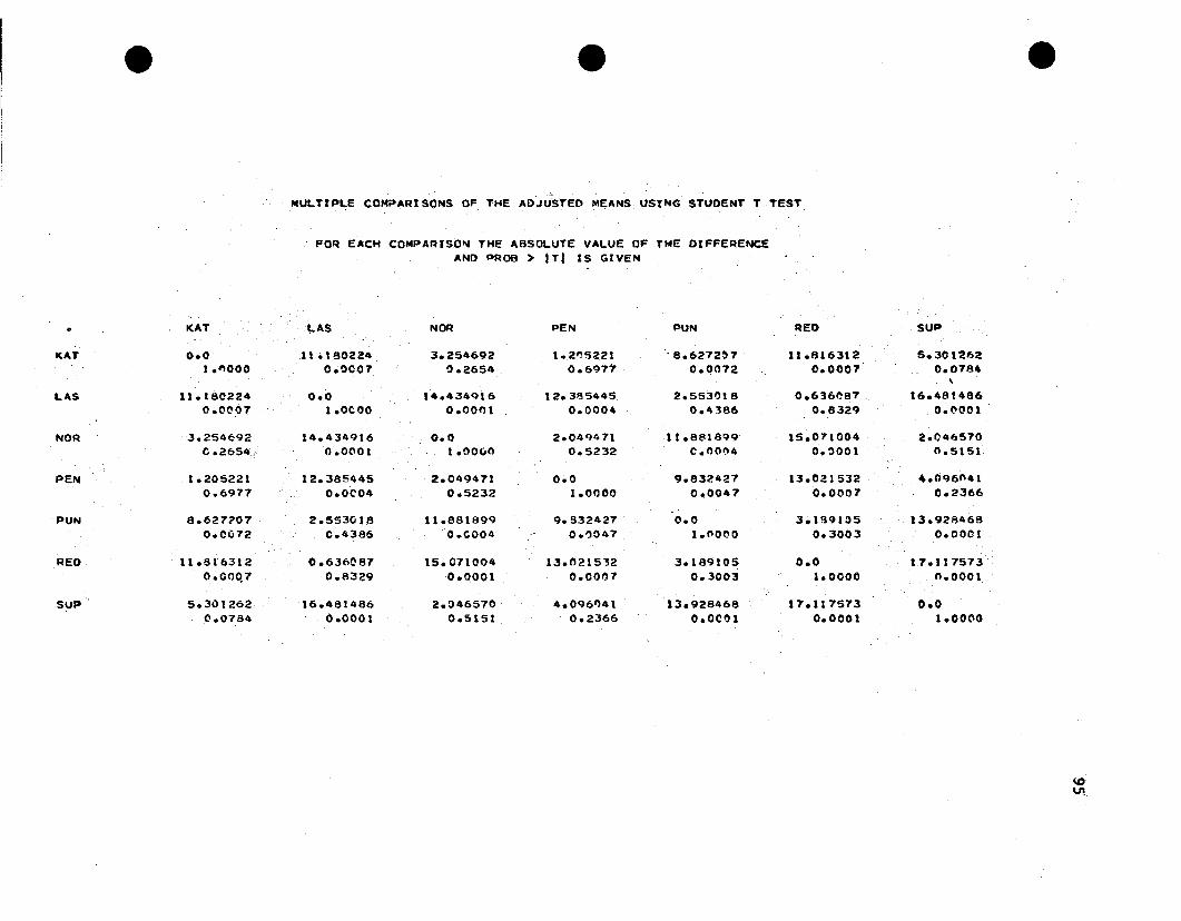
e e

MULTIPLE COM;:>ARI SONS OF THE AD)U'STED MEANS USING STUDENT T TEST

FOR EACH COMPARISO~ THE ABSOLUTE VALUE OF TME DIFFERENCEAND PROS> ITI IS GIVEN

e

I(AT LAS NOR pEN PUN REO SUP

KAT 0.0 1\ .180224 3.254692 1.2~S221 '8.6272'7 11.816312 5.3012621."000 0.0007 0.2654 0.6977 0.0072 0.0007 0.078"

LAS 11.18C224 0.0 14.434916 12.385"45 2.5531)18 0.636"87 16.4814860.0(,\07 1.0eoo 0.0001 0.0004 0.4386 0.8329 0.0001

NOR 3.254e-92 14.434916 0.0 2.04Q471 11.881899 15.071004 2.046570C .2654, 0.0001 1.00liO 0.5232 C.OOI.'4 0.0001 n.5151

PEN 1.205221 12.385445 2.049471 0.0 9.832427 13.021532 4.096(\410.6977 0.OC04 0.5232 1.0000 0.0047 0.0007 0.2366

PUN 8.627?07 2.553011'1 11.881899 9.632427 0.0 3.189105 13.9284680.0072 0.4386 0.C004 0.')047 1.(\0(,\0 0.3003 0.0001

REO 11.816312 0.636087 15.071004 13.021532 3.18<)105 0.0 11.117573a.ooq7 0.8329 0.0001 0.0007 0.3003 1.0COO n.OOOI

SUP 5.301262 16.481486 2.046570 ' 4.0(61)41 13.928468 17.117573 0.00.0784 0.0001 0.5151 0.2366 O.OC!)1 0.0001 1.0000

~

~,

ALL POSSIBLE STANOARD eRRO~ OF DIFFERe"'CES BETWEEN AOJ.USTEO MEANS

KAT LAS NOR PFlIl PUN RED SOP

KAT 0.0 2.962522 2.867568.

3.073307 2.990646 3.130495 ·2,.908995

LAS 2.962522 0.0 2.844069 3.093336 3.252003 2.9~9013 3.(\19176

NOR 2.867568 2.844C69 0.0 3.172609 2.995900 3.087609 3.106725

PEN 3.073307 3.093336 3.172609 0.1} 3.219672 3.422491 3.391283

PUN 2.990646 3.252003 2.995900 3.219672 0.0 3.025796 ' 3.125210

RED 3.130495 2.989013 3.087609 3.422491 3.025796 0.0 3.268608

5UP .2.908995 3.019176 3.106725 3.391283 3.125210 3.268.608 0.0

\00\

e e e

e e

8.2. Comparison of Known with Estimated Treatment EffectsObtained From Unadjusted and Adjusted Treatment MeansUsing the Siwa1ated Data.

e

Trt. Treatment Upper Half Lower Half Upper Half Lower Half Upper ·-Half ,Lower HalfDesign No. Effect Unadj. Adj. Unadj. Adj. Unadj. Adj. Unadj. Adj. Unadj.: Adj. Unadj. Adj.

CR 1 1 -7.0 1.0 -5.6 1.0 -2.6 0~7 -1.2 1.4 2.3 1.0 2.2 0.82 2 -6.7 2.3 -2.7 2.1 -2.3 1.7 2.0 1.9 9.2 2.0 9.3 2.23 3 8.2 2.9 8.0 2.9 5.5 3.6 5.3 3.0 3.3 3.3 3.0 3.04 3 6.4 2.9 6.9 3.0 4.2 3.1 4.8 3.1 3.0 3.0 3.2 3.25 2 8:'2 2.0 5.2 2.0 4.2 2.1 1.8 1.9 0.2 1.9 0.3 1.96 0 1.8 -0.1 -0.7 0.2 1.2 0.0 -1.3 0.2 -6.3 0.0 -6.3 -0.1

RCB 1 1 7.0 0.8 -5.7 1.4 4.1 1.0 1.2 0.9 -2.4 1.1 -2.5 1.02 2 -1.6 1.9 -2.8 2.0 0.3 1.8 2.2 1.8 5.4 1.9 5.4 1.93 3 11.6 3.2 7.9 3.2 6.0 2.8 2.8 2.9 -4.1 3.0 -4.2 2.84 3 -5.7 3.2 6.8 2.6 -0.5 3.0 2.0 3.2 9.2 3.0 9.2 3.15 2 2.1 1.8 5.1 2.1 2.4 2.1 2.5 1.9 2.2 2.2 2.0 2.06 0 -2.6 -0.1 -0.8 -0.2 -1.6 -0.1 0.3 -0.2 0.7 -0.2 1.0 0.0

LS 1 1 1.3 1.3 0.4 0.2 1.0 1..1 0.3 1.0 0.8 0.7 0.9 1.12 2 4.3 2.4 2.0 2.0 4.5 2.3 1.7 1.9 1.9 1.9 2.0 2.43 3 3.6 3.0 3.6 3.9 4.0 3.3 3.5 3.0 3.0 3.1 3.0 3.14 3 2.5 2.9 3.6 4.0 2.5 3.0 3.8 3.3 3.0 3.1 2.8 2.65 2, 0.6 1.7 2.0 2.0 0.6 1.8 2.1 2.0 2.0 2.0 2.1 1.96 .0 -1.6 -0..7 -0.7 1.1 -1.5 0.7 -0.5 -0.1 0.1 0.0 0.1 -0.1

'0"-J

8.3. Estimates of Error Variance Using Standard DesignAnalysis and Trend Analysis for Different Yield Responses.

Field: E-3 Field: L-2

Yield of Design Standard Trend Standard Trend

Size A CR 20.163 6.428 73.037 20.712

Tubers R.CB 14.394 5.353 49.464 18.420

LS 10.017 7.276 12.815 11.208

Unif. 8.685 8.986

Size B CR ..1.1224 .6329 2.7698 1.1688

Tubers RCB .7168 .3884 2.7320 1.7493

LS .8143 .5459 1.6121 1.4942

Unif. .• 5271 .9401

Culls CR 2.1041 1.3200 3.6703 2.1652

RCB 1.9042 1.1975 2.8435 2.2196

LS 1.6621 1. 2837 3.1037 1.4341

Unif. .9575 3.3578

Marketable CR 23.337 7.218 93.673 24.217

RCB 16.415 6.8q·l 58.967 19.367

LS 11. 749 8.634 13.604 13.090

Unif. 6.517 11. 758

98

8.4. Percent Gain in Relative Efficiency Due to Designor Trend Analysis Using Estimates of Error Variancefor Different Yield Responses.

Field: E-3 Field: L-2

Yield of Design RCB L8 ..Trerld RCB L8 'Trend

Size A CR 39.1 97.9 208.4 46.6 496.5 248.6

Tubers RCB 42.3 166.3 282.2 166.9

LS 37.7 14.7

Size B CR 55.5 35.5 75.3 0.6 68.9 133.8

Tubers ReB 0.0 82.7 67.8 55.9

LS 49.7 8.3

Culls CR 9.7 24.4 58.9 28.1 16.2 67.3

RCB 13.4 57.4 0.0 27.1

L8 30.2 116.4

Marketable CR 41.1 95.3 217.8 57.7 576.9.282.3.,

Yield RCB 38:3 138:9 329:2 201:5

LS 36.1 4.5

99

100

8.5. Ranked Cultivar Means (Before and After Adjusting forTrend) Using Yield of Size A Tubers from Field E-3.

Unadjusted Adjusted

Design Cultivar Means Cultivar Means

CR Superior 12.71

IISuperior 13.50

Norchip 16.36 Norchip 13.86

Penn-71 20.86 Katahdin. 21.14

IKatahdin 22.07 Penn-71 21.63

Pungo 26.57 Pungo 27.89

Lasoda 29.79 Lasoda 30.28

Red. Pontiac 30.86 Red Pontiac 30.92

RCB Norchip 12.21 Nochip 12.38 ISuperior 12.50 Superior 13.49

Katahdin 15.93

IIKatahdin 18.48

IPenn-71 20.00 Penn-71 18.88

Pungo 22.14 Pungo 22.21

Lasoda 27.43 Lasoda 26.98

Red Pontiac 30.71 Red Pontiac 28.67

LS Norchip 12.64 Norchip 11.33

Superior 14.29 Superior 15.07

Penn-71 15.36 Penn-71 15.36 .

Katahdin 17.79 Katahdin 17.00

Pungo 23.21 Pungo 24.53

Lasoda 28.14 Lasoda 26.39

Red Pontiac 29.14 Red Pontiac' 30.89

Note:

Any two means not joined by the same line are significantly different.Any two means joined by the same line are not significantly different.

8.6. Ranked Cu1tivar Means (Before and After Adjesti!lg forTrend) Using Yield of Size A Tubers from Field L-2.

101

Unadjusted Adjusted

Design Cu1tivar Means Cultivar Means

CR Superior 18.07 I Superior 16.92

Norchip 19.07 Norchip 17.22

Katahdin 23.43 Katahdin 23.92

IPenn-71 26.64 Penn-71 25.18

Pungo 28.29 Pungo 30.27

IIRed Pontiac 32.57 Red Pontiac 35.16

Lasoda 36.79 Lasoda 36.18

ReB Norchip 20.79 Superior 22.54

Superior 22.14 Norchip 22.94

Katahdin 27.86 Katahdin 25.23

IIPenn-71 29.00 Penll-71 29.65

Red Pontiac 34.64 Pungo 33.32

IPungo 36.50 Red Pontiac 35.37

Lasoda 40.07 Lasoda 41.94

LS Norchip 20.14 Norchip 19.32

I,Superior 20.50 Superior 21.99

Katahdin 24.00

I,Penn-71 24.41

I,Penn-71 26.29 Katahdin 25.87

Pungo 29.86 Pungo 28.37

Lasoda 37.50 Lasoda 38.33

Red Pontiac 42.00 Red Pontiac 42.00

Note:

Any two means not joined by the same line are significantly different.Any two means joined by the same line are not significantly different.

102

8.7. Ranked Cultivar Means (Before and AfterAdjusting for Trend) Using Yield of SizeB Tubers from Field E-3

Una.djusted Adjusted

Design Cultivar Means Cultivar Means

CR Penn-71 1.97 Perm-71 1..77

Katahdin 3.17 Katahdin 3.11

Lasoda 3.94 Lasoda 4.28

Pungo 4.26, Red Pontiac 4.62

Superior 4.79 Pungo 4.70

Red Pontiac 5.03 Superior l+.80

Norehip 7.36 Norchip 7.21

RCB Penn-71 1.54 Penn-71 1.09

Katahdin 2.34 Katahdin 2.13

Pungo 3.10 Lasoda 3.06

Lasoda 3.21 Pungo 3.16

Superior 3.69 Superior 4.05

Red Pontiac 4-.86 Red Pontiac 5.40

Norchip 6.20 Norchip 6.03

LS Penn-71 1. L,·9 Penn-71 1.49

Katahdin 2.54- Kata.hdin 2.85 !Pungo 2.89 Pungo 3.13 I iSuperior 4.20 Superior 3.90 I

I

Red Pontiac 4.20 Red Pontiac II.IS

Lasoda 4.20 Lasoda {L26

Norchip 6. 9l~ Norccip 6.70

Note:

Any two means not joined by the same line are sig!".ificantly diffe!'ent.Any two mea.ns joined by the same line are not significantly different.

103

8.8. Ranked Cu1tivar Means (Before and After Adjustingfor Trend) Using Yield of Size B Tubers from Field L-2.

Unadjusted Adjusted

Design Cu1tivar Means Cultivar Means

CR Penn-71 1.51 Penn-71 1.32

Katahdin 3.31 Katahdin 3.49

Red Pontiac 4.03 Lasoda 3.87

Lasoda 4.11 Pungo 5.05

Superior 5.36 Red Pontiac 5.13

Pungo 5.47 Superior 5.55

Norchip 8.00 Norchip 7.40

RCB Penn-71 1.40 Penn-71 1. 26

Katahdin 3.34 Katahdin 2.90

Lasoda 4.39 Red Pontiac 4.34

Red Pontiac 4.44 Lasoda 4.74

Superior 4.93 Superior 5.19

Pungo 5.79 Pungo 5.72

Norc1i;i.p 6.83 Norchip 6.96

LS Penn-71 1.27 Penn-71 1.18

Katahdin 2. 841

Katahdin 2.75

Pungo 3.91 Pungo 04·.01

Superior 4.79 Lasoda 4.62

Lasoda 4.80 Superior 4.88

Red Pontiac 5.29 Red Pontiac 5.65

Norchip 6.66 Norchip 6.48

Note:

Any two means not joined by the same line are significantly different.Any two means joined by the same line are not significantly different.

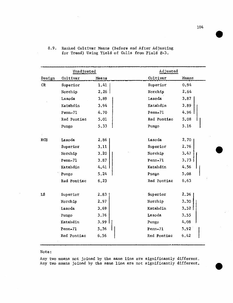
104

8.9. Ranked Cultivar Means (Before and After Adjustingfor Trend) Using Yield of Culls from Field E-3.

Unadjusted Adjusted

Design Cu1tivar Means Cu1tivar Means

CR Superior 1.41 Superior 0.94

Norchip 2.26 Norchip 2~64

Lasoda 3.89 Lasoda 3.87

Katahdin 3.94 Katahdin 3.89

Penn-71 4.70 Penn-71 4.96

Red Pontiac 5.01 Red Pontiac 5.08

Pungo 5.33 Pungo 5.16

RCB Lasoda 2.86 Lasoda 2.70

Superior 3.11 Superior 2.76

Norchip 3.20 Norchip 3.47

Penn-71 3.87 Penn-71 3.73

Katahdin 4.41 Katahdin 4.56

Pungo 5.24 Pungo 5.08

Red Pontiac 6.23 Red Pontiac 6.63

LS Superior 2.83 Superior 2.36

Norchip 2.97 Norchip 3.30

Lasoda 3.69 Katahdin 3.52

Pungo 3.76 Lasoda 3.55

Katahdin 3.99 Pungo 4.08

Penn-71 5.36 Penn-71 5.92

Red Pontiac 6.56 Red Pontiac 6.42

Note:

Any two means not joined by the same line are significantly different.Any two means joined by the same line are not significantly different.

105

8.10. Ranked Cul.tivar Means (Before and. After Adjustingfor Trend) Using Yield of Culls from .Field L-2.

Unadjusted Adjusted

Design Cultivar Means Cultivar Means

CR Lasoda 3.53 Lasoda 3.74

Red Pontiac 4.30 Norchip 4.66

Superior 4.81 Red Pontiac 4.92

Norchip 5.03 Superior 5.24

Penn-71 5.99 Penn-71 5.31

Katahdin 6.23 Katahdin 6.41

Pungo 8.63 Pungo 8.24

RCB Superior 2.56 Superior 2.58

Red Pontiac 3.86 Red Pontiac 3.85

Lasoda 3.87 Norchip 4.04

Norchip 4.37 Lasoda 4.17

Pungo 4.93 Pungo 4.76

Penn-71 5.27 Penn-71 5.33

Katahdin 6.49 Katahdin 6.61

LS Lasoda 3.00 Lasoda 2.37

IISuperior 3.20 Norchip 3.25

Norchip 3.89 Superior 3.89

Red Pontiac 4.81 Katahdin 5.32

Pungo 5.49 Red Pontiac 5.57

Katahdin 5.76 Pungo 6.18

Penn-71 6.66 Penn-71 6.22

Note:

Any two means not joined by the same line are significantly different.Any two means joined by the same line are not significantly different.

106

8.11. Ranked Cultivar Means (Before and After Adjustingfor Trend) Using Marketable Yield from Field E-3.

Unadjusted Adjusted

Design Cultivar Means Cultivar Means

CR Superior 17.50 Superior 18.84

Penn-71 22.83 Norchip 21.35

Norchip 23.71 Perm-71 23.19

Katahdin 25.24 Katahdin 24.49

Pungo 30.81 Pungo 32.36

Lasoda 33.73 Lasoda 34.72

Red Pontiac 35.89 Red Pontiac 34.76

RCB Superior 16.19 Superior 16.04

Katahdin 18.27 Norchip 19.40

Norchip 18.41 Penn-71 20.09

Penn-71 21.51 Katahdin 21.50

Pungo 25.24· Pungo 24.76

Lasoda 30.64 Lasoda 30.39

Red Pontiac 35.57 Red Pontiac 33.67

LS Penn-71 16.84 Penn-71 16.84

Superior 18.49 Norchip 18.15

Norchip 19.59 Superior 19.32

Katahdin 20.33 Katahdin 1.9.50

Pungo 26.10 Pungo 27.54

Lasoda 32.34 Lasoda 30.48

Red Pontiac 33.34 Red Po~tie,c 35.21

Note:

Any two means not joined by the saIne line are significantly different.Any two means joined by the same line are not significantly different.

8.12. Ranked Cultivar Means (Before and After Adjustingfor Trend) Using Marketable Yield from Field L-2.

Unadjusted Adjusted

Design Cultivar Means Cu1tivar Means

CR Superior 23.43 Superior 22.16

Katahdin 26.74 Norchip 24.84

Norchip 27.07 Penn... 71 26.61

Penn..71 28.16 Katahdin 27.32

Pungo 33.76 Pungo 35.83

Red Pontiac 36.60 Red Pontiac 39.75

Lasoda !j·0.90 Lasoda 40.15

RCB Superior 27.07 Superior 26.41

Norchip 27.61 Norchip 28.3!j.

Penn..71 30.40 Katahdin 30.14

Katahdin 31.20 Penn..71 32.11

Red Pontiac 39.09 Red Pontiac 39.04

Pungo 42.29 Pungo 40.02

Lasoda 44.46 Lasoda 46.06

LS Superior 25.29 Superior 26.19

Norchip 26.80 Norchip 26.44

Katahdin 26.84 Penn..71 26.65

Penn-71 27.56 Katahdin 27.50

Pungo 33.77 Pungo 32.87

Lasoda 42.30 Lasoda 42.66

Red Pontiac 47.29 Red Pontiac 47.29

107

---Note:

Any two means not joined by the same line are significantly different.Any two means joined by the same line are not significantly different.