MILITARY HANDBOOK DESIGN HANDBOOK - MIL-STD...
562
MIL-HDBK-416 15 NOVEMBER 1977 MILITARY DESIGN HANDBOOK HANDBOOK FOR LINE OF SIGHT MICROWAVE COMMUNICATION SYSTEMS SLHC Downloaded from http://www.everyspec.com
-
Upload
duongquynh -
Category
Documents
-
view
226 -
download
1
Transcript of MILITARY HANDBOOK DESIGN HANDBOOK - MIL-STD...

MIL-HDBK-41615 NOVEMBER 1977
MILITARY
DESIGN
HANDBOOK
HANDBOOKFOR
LINE OF SIGHT MICROWAVE
COMMUNICATION SYSTEMS
SLHC
Downloaded from http://www.everyspec.com

MIL-HDBK-41615 NOVEMBER 1977
DEPARTMENT OF DEFENSEWASHINGTON 25, D.C.
Design Handbook for Line of Sight Microwave Communication System
1. This standardization handbook was developed by the Department ofDefense in accordance with established procedure.
2. This publication was approved on 15 November 1977 for printingand inclusion in the military standardization handbook series.
3. This document provides basicof sight radio system It will
and fundamental information on lineprovide valuable information and
guidance to Personnel concerned with the preparation of specificationsand the procurement of line of sight radio systems. The handbook isnot intended to be referenced in purchase specifications except forinformation purposes, nor shall it supersede any specification re-quirements.
4. Benficial comments (recommendations, additions, deletions) andany pertinent data which may be of use in improving this documentshould be addressed to:
CommanderRome Air Development CenterATTN: RADC/RBRDGriffiss APB, NY 13441
Downloaded from http://www.everyspec.com

MIL-HDBK-41615 NOVEMBER 1977
This handbook provides considerations for use in the design,installation, operation and acceptance of Department of Defense(DOD)long haul DCS Line-of-Sight (LOS) analog microwave communicationsfacilities.
iii
FORWARD
Downloaded from http://www.everyspec.com

Downloaded from http://www.everyspec.com

MIL-HDBK-41615 NOVEMBER 1977
CONTENTS
CHAPTER 1. SCOPE
Section 1.1 General
1.2 Purpose
1.3 Application
1.4 Objectives
1.5 General Insrtuctions
1.6 Organization
CHAPTER 2. REFERENCED DOCUMENTS
CHAPTER 3. TERMS AND DEFINITIONS
Section 3.1 Symbols
CHAPTER 4. SYSTEM DESIGN
Section 4.0 Introduction
4.1 Starting Design
4.1.1 General
4.1.2 Functional Requirements
4.1.3 Channel parameters
4.1.4 Resource Limitations
4.1.5 Economic Restraints
4.1.6 Real Estate Availability
4.1.7 Construction Limitation
4.1.8 Primary Power Limitations
4.1.9 Frequency Spectrum Availability
4.1.10 Radio Frequency Assignment
Page1-1
1-1
1-2
1-2
1-3
1-4
1-4
2-1
3-1
3-1
4-1
4-1
4-3
4-3
4-3
4-4
4-7
4-7
4-8
4-8
4-9
4-9
4-10
v
Downloaded from http://www.everyspec.com

MIL-HDBK-41615 NOVEMBER 1977
Contents
4.1.11
4.1.13
4.1.14
4.1.15
Application for Frequency Allocation
Engineering Implementation Plan (EIP)Contents and Organization
EIP Deadlines and Schedules
Determine Basic Feasibility
Review Requirements vs. Limitations
Section 4.2 Study of Route Alternatives
4.2.1
4.2.2
4.2.3
4.2.4
4.2.5
4.2.6
4.2.7
4.2.8
4.2.9
4.2.10
4.2.11
4.2.12
4.2.13
4.2.14
4.2.15
4.2.16
4.2.17
General
Select Potential Sites
Eliminate Non-available Areas
Obtain Best Available Maps
Preliminary Site Selection
Select
Choose
Choose
Potential Routes
Potential Relay Links
Direct Routes
Consider Passive Repeaters
Consider the Number of Sites
Atmospheric Layer Pentration
Select preliminary Routes
Drawing Initial Terrain Profiles
Map Scale
Initial Path Profile Drawings
Plotting a Great Circle Path
Path Clearancevi
Page
4-11
4-11
4-16
4-16
4-18
4-19
4-19
4-19
4-19
4-20
4-22
4-23
4-25
5-25
4-27
4-28
4-28
4-29
4-30
4-30
4-33
4-36
4-39
4.1.12
Downloaded from http://www.everyspec.com

MIL-HDBK-41615 NOVEMBER 1977
Contents
4.2.18 Fresnel Zones
4.2.19 Terrain Reflections
4.2.20 Initial Path Loss Estimates
4.2.21 Free Space Basic Transmis-sion Loss and Free SpacePath Loss
4.2.22 Atmospheric Absorption
4.2.23 Attenuation Due toPrecipitation
4.2.24 Estimating Rain Attenuation
4.2.25 Atmospheric Refraction
4.2.26 Multipath Fading
4.2.27 Estimating Multipath Fading
4.2.28 Combining Path Loss Contribut-ions and Grading Paths
4.2.29 Fading Estimates for LongLOS Links
4.2.30 Additional Route Considerations
4.2.31 Meteorological and Climate-logical Data
4.2.32 Tower Height
4.2.33 Radio Interference
4.2.34 Site Security
4.2.35 Select Primary and AlternateRoutes
4.2.36 Path Loss Measurements
Section 4.3 Field Survey
4.3.1 General
4.3.2 Planning The Field Survey
4.3.3 List Information Required
vii
Page
4-40
4-43
4-44
4-45
4-46
4-48
4-50
4-59
4-61
4-63
4-64
4-65
4-68
4-68
4-71
4-72
4-73
4-74
4-74
4-76
4-76
4-77
4-78
Downloaded from http://www.everyspec.com

MIL-HDBK-41615 NOVEMBER 1977
ContentsPage
4. 3.4
4. 3.5
4. 3.6
4. 3.7
4. 3.8
4. 3.9
4.3.10
4.3.11
4.3.12
4.3.13
4.3.14
4.3.15
4.3.16
4.3.17
4.3.18
4.3.19
4.3.20
4.3.21
4.3.22
4.3.23
Survey Equipment Require-ments 4-88
Transportation 4-89
Personnel 4-90
Frequency Requirements 4-90
Time Requirements 4-91
Request for Survey 4-91
Obtain Permission for SiteVisits 4-91
Site Visits 4-93
Survey Terrain Clearances 4-98
Profiles from AltimeterSurveys 4-98
Profiles from Optical Surveys 4-100
Profiles from Aerial Surveys 4-100
Profiles from New Maps Drawnfrom Aerial Photographs 4-101
Path Loss Measurements 4-102
Objectives of Path Loss Tests 4-104
Antenna Height Gain, Lobing,and Atmospheric Effects 4-104
Verification of Line-of-SightConditions 4-105
Selecting Optimum AntennaHeights by Path Loss Tests 4-106
Evaluation of Fading Phenomenaand Diversity Design 4-107
Utilization of Survey andMeasurement Data 4-110
viii
Downloaded from http://www.everyspec.com

MIL-HDBK-41615 NOVEMBER 1977
Contents
Section 4.4 Link Design
4.4.1
4.4.2
4.4.3
4.4.4
4.4.5
4.4.6
4.4.7
4.4.8
4.4.9
4.4.10
4.4.11
4.4.12
4.4.13
4.4.14
4.4.15
4.4.16
4.4.17
4.4.18
4.4.19
4.4.20
General
The Link Design Estimate
Path Profile Upgrading andChecking
Calculating Tower Heights
Line-of-Sight Propagationover Smooth Earth andIrregular Terrain
Refractive Index Gradients
Determination of the Range ofRefractivity Gradients
Fading Mechanisms
Multipath Fading
Multipath Characteristics
Power Fading
Power Fading due toDiffraction
Power Fading due“Decoupling”
Power Fading dueand Layers
to Antenna
to Ducts
Fading due to Precipitation
Combinations of FadingMechanisms
k-type Fading
Surface Duct Fading
The Relative Amplitudes ofthe Multipath Components
The Received Signal AmplitudeDistributions
Page
4-112
4-112
4-113
4-115
4-122
4-125
4-126
4-133
4-137
4-137
4-142
4-143
4-144
4-149
4-151
4-152
4-152
4-152
4-155
4-159
4-160
ix
Downloaded from http://www.everyspec.com

MIL-HDBK-416
Contents
4.4.21
4.4.22
4.4.23
4.4.24
4.4.25
4.4.26
4.4.27
4.4.28
4.4.29
4.4.30
4.4.31
4.4.32
4.4.33
4.4.34
4.4.35
4.4.36
4.4.37
4.4.38
4.4.39
4.4.40
4.4.41
Path Fading
Diversity onLinks
Range Estimates
Microwave Relay
A Comparison of Frequencyand Space Diversity
Engineering Considerations
Combiners
Radio Frequency Interferenceand Radio Noise
Selective Interference
Equipment considerations
Antennas
Mechanical Stability ofAntennas
Passive Repeaters
Gain and Radiation Patternsof Flat Reflectors
Conditions of Planarity forReflectors
Radio Path with Single FlatReflector
Two Flat Reflectors in OnePath
Two Flat Reflectors to ChangeBeam Directions
Parabolic Antennas Back-to-Back
Periscope Antennas
Diffractors as PassiveRepeaters
RF Transmission Lines
Coaxial Cable
Page
4-168
4-171
4-177
4-180
4-181
4-182
4-186
4-187
4-188
4-202
4-203
4-204
4-205
4-205
4-206
4-207
4-208
4-208
4-209
4-210
4-210
x
Downloaded from http://www.everyspec.com
MIL-HDBK-41615 NOVEMBER 1977
Contents
4.4.42 Waveguide
4.4.43 Microwave Separating andCombining Elements
4.4.44 Transmitters
4.4.45 Receivers
4.4.46 Active Repeaters
Section 4.5 Integrating Link Design into SystemDesign
4.5.1
4.5.2
4.5.3
4.5.4
4.5.5
4.5.6
4.5.7
4.5.8
4.5.9
4.5.10
4.5.11
4.5.12
4.5.13
4.5.14
General
System Layout
Site Radio EquipmentRequirements
Frequency Compatibility
General Aspects of FrequencyAllocation
References to AppropriateSections of the RadioRegulations
Choice of One or more Fre-quencies from those Avail-able in the Radio-frequencyChannel Arrangement
The Production and the Effectsof Unwanted Couplings
Types of Interference
Co-channel Interference
Adjacent Channel Interference
Direct Adjacent ChannelInterference
Other Sources of Interference
Hop/System Noise Perform-ance Estimates
xi
Page
4-212
4-214
4-216
4-221
4-225
4-231
4-231
4-232
4-237
4-239
4-239
4-239
4-240
4-245
4-247
4-248
4-252
4-252
4-253
4-254
Downloaded from http://www.everyspec.com
MIL-HDBK-41615 NOVEMBER 1977
Contents
4.5.15
4.5.16
4.5.17
4.5.18
4.5.19
4.5.20
4.5.21
4.5.22
4.5.23
4.5.24
4.5.25
4.5.26
4.5.27
4.5.28
4.5.29
4.5.30
DCS Noise Requirements
Calculate Hop NoiseAllowance
Select Basic EquipmentParameters
Path Loss Distribution
Select Antenna Size, Transmis-sion Line, TransmitterPower, and Calculate Long-term Median ReceiverInput Power
Equipment IntermodulationNoise Calculation
Feeder IntermodulationNoise Calculation
Time-invariant NonlinearNoise
Thermal Noise
Points at which ThermalNoise Power canInfluence the Signal
The Mechanism by which theThermal Noise Power canInfluence the Signal
Pre-emphasis
Calculate Long-term MedianThermal Noise
Determine Long-term MedianTotal Noise Performance
Compare Hop Predicted Noisewith Noise Allowance
Adjust Hop/ EquipmentRequirements
Page
4-254
4-254
4-261
4-275
4-276
4-280
4-284
4-293
4-293
4-295
4-295
4-295
4-296
4-299
4-299
4-299
xii
Downloaded from http://www.everyspec.com

Contents (continued)
4.5.31 Estimate Short-term SignalLevels at the ReceiverInput
4.5.32 Rain Attenuation
4.5.33 Multipath Fading
4.5.34 Diversity
4.5.35 Complete System SummaryCharts
4.5.36 System Reliability
4.5.37 Reliability Calculations
4.5.38 A Practical Example of LOSSystem Reliability
4.5.39 Causes of System Outage
4.5.40 Designing for Reliability
4.5.41 Examples of Filled-inWorksheets
CHAPTER 5. FACILITY DESIGN
Section 5.0 Introduction
5.1 Site Planning
5.1.1 General
5.1.2 Site Plan
5.1.3 Access Roads
5.1.4 Site Preparation
5.1.5 Building Design
5.1.6 Station Ground
Section 5.2 Equipment Layout
MIL-HDBK-41615 NOVEMBER 1977
Page
4-300
4-300
4-301
4-302
4-306
4-306
4-307
4-308
4-308
4-308
4-311
5-1
5-1
5-2
5-2
5-5
5-11
5-11
5-11
5-19
5-23
xiii
Downloaded from http://www.everyspec.com

MIL-HDBK-41615 NOVEMBER 1977
Contents (continued)5.2.1 General
5.2.2 Installation Plans
Section 5.3 PRIME AND AUXILIARY POWER
5.3.1 General
5.3.2 Description of ElectricalPower System
5.3.2.1 Primary Source
5.3.2.2 Emergency Source
5.3.2.3 Floating Battery“Class D“
Plant
5.3.4 Fuel Storage Facility
Section 5.4 TOWER REQUIREMENTS
5.4.1 General
5.4.2 Structural Design
5.4.3 Tower Safety
5.4.4 Lightning Protection For Towers
5.4.5 Painting And LightingRequirements
Section 5.5 ENVIRONMENT CONTROL
5.5.1 General
5.5.2 Environment Condition-ElectronicEquipment Spaces
5.5.4 Design Conditions-AuxiliaryEquipment
Section 5.6 TRANSMISSION LINES5.6.1 General
5.6.2 Waveguide
5.6.3 Waveguide
5.6.4 Waveguide
xiv
Rooms
Types
Layout and Installation
Components
Page5-23
5-26
5-31
5-31
5-31
5-31
5-31
5-32
5-32
5-33
5-33
5-33
5-38
5-39
5-40
5-44
5-44
5-45
5-46
5-485-48
5-48
5-51
5-53
Downloaded from http://www.everyspec.com

MIL-HDBK-41615 NOVEMBER 1977
Section 5.7 AUXILIARY EQUIPMENT FOR OPERATIONAL/MAINTENANCE
5.7.1 Fault Alarm Systems
5.7.2 Maintenance Communicationand Orderwire
Section 5.8 ELECTROMAGNETIC COMPATIBILITY
5.3.1 General
5.8.2 EMC Problems To be ExpectedIn Microwave Systems
5.8.3 Engineering Team Approach
CHAPTER 6. ADDITIONAL ENGINEERING PROCEDURES
Section 6.0 Introduction
Section 6.1 Determination of Azimuth from Observations
of Polaris
6.1.1 Introduction
6.1.2 Observational Procedures
6.1.3 Determination of Local Mean Time
6.1.4 Hour Angle Determination
6.1.5 Azimuth of Polaris
Page5-54
5-54
5-56
5-59
5-59
5-62
5-64
6-1
6-1
6-1
6-1
6-4
6-5
6-8
6-9
6.1.6 Observation of Polaris by the ElongationMethod 6-10
6.1.7 Checking the Azimuth 6-11
Section 6.2 Determination of Elevation by AltimeterSurvey 6-12
Section 6.3 Opical Methods of Checking Radio-pathObstructions 6-19
6.3.1 Introduction 6-19
Section 6.4 Equipment, Towers, Calibrations, and TestProcedures for Path-loss Measurements
6.4.1 Introduction
6.4.2 Characteristics of the RadioEquipment
6-23
6-23
6-23xv
Downloaded from http://www.everyspec.com

MIL-HDBK-41615 NOVEMBER 1977
6.4.3 Typical Test Link
6.4.4 Test-towers
6.4.5 Associated Test Equipment
6.4.6
6.4.7
6.4.8
6.4.9
6.4.10
6.4.11
6.4.12
6.4.13
6.4.14
6.4.15
6.4.16
6.4.17
6.4.18
6.4.19
Antenna Carriage
Power Requirements
Licensing of RadioEquipment
Manpower Requirements
Calibrations
Radio-frequency Levels in aRadio Path
Typical Calibration Procedure
Sample Calculation
Calibration Errors
Suggested Test Procedure
Suggested Sequence of Tests
Worst Combinations of AntennaHeights
Test Frequency
Signal-level Recording
Section 6.5 Path Loss Calculations for Single KnifeEdge Diffraction Links
6.5.1 Introduction
6.5.2 Required Atmospheric Parameters
6.5.3 Required Terrain Parameters
6.5.4 Attenuation Over IsolatedDiffracting Ideal Knife Edge
6.5.5 Effects of Ground Reflections
6.5.6 Attenuation Over a RoundedKnife Edge
xvi
Page6-23
6-24
6-28
6-28
6-29
6-29
6-30
6-30
6-30
6-31
6-32
6-33
6-34
6-34
6-35
6-35
6-35
6-37
6-37
6-38
6-42
6-44
6-46
6-55
Downloaded from http://www.everyspec.com

Contents
Section
Chapter 7.
Figure
1-1
1-2
1-3
1-4
1-5
4.1-1
4.2-1
4.2-2
4.2-3
4.2-4
MIL-HDBK-41615 NOVEMBER 1977
Page
6.5.7 Fading and Long-Tern Variability 6-61
6.5.8 Worksheets for Diffraction Calctiationand An Example 6-64
6.6 Additional Blank Worksheets6-75
INDEX OF KEY TERMS7-1
FIGURES
Title
FlOW Chart for Section 4.1 (Starting Design)
Flow Chart for Section 4.2 (Study of RouteAlternatives)
Flow Chart for Section 4.3 (Field Survey)
Flow Chart for Section 4.4 (Link Design)
Flow Chart for Section 4.5 (Integrating LinkDesign into System Design)
Dependence of RF Bandwidth on BasebandWidth for FDM-FM Systems
Nominal Path Lengths for Line-of-Sight Pathsbetween 8 and 40 GHz without ParallelRoute Diversity
Typical Passive Repeater Configuration
Grid Zone Designation for the World
Typical Flat Earth Path Profile
1-5
1-6
l-7
1-8
1-9
4-6
4-26
4-28
4-32
4-35
xvii
Downloaded from http://www.everyspec.com

MIL-HDBK-41615 NOVEMBER 1977
Figures (continued)Figure Title
4.2-5 Spherical Triangle for Great Circle PathComputations
4.2-6 Fresnel Zone Geometry
4. 2-7 Free Space Basic Transmission Loss versusPath Length
4.2-8 Surface Values yoo and ywo of Absorption byOxygen and Water Vapor
4.2-9 Rain Attenuation versus Rainfall Ratebetween 5 and 100 GHz
4.2-10 Rainfall Rate-time Distributions for SixClimatic Zones
4.2-11 Zones of Maximum Five-Minute RainfallRates
4.2-12a Time Distributions of Rain Attenuationper Kilometer of Path Length for RainRate Zones 1 and 2
4.2-12b Time Distributions of Rain Attenuationper Kilometer of Path Length for RainRate Zones 3 and 4
4.2-12c Time Distributions of Rain Attenuationper Kilometer of Path Length for RainRate Zones 5 and 6
4.2-13 World Rain Rate Zones
4.2-14 Fading Allowances for Long Line-of-Sight Paths
4.3-1 Section of Topographic Map Showing"Mesa"Site (USGS Lyons, Colo. 7 1/2’ quadrangle)
Page
4-37
4-41
4-47
4-49
4-52
4-53
4-54
4-55
4-56
4-57
4-58
4-67
4-82
xviii
Downloaded from http://www.everyspec.com

Figures (continued)Figure
4.3-2
4.3-3
4.4-1
4.4-2
4.4-3
4.4-4
4.4-5
4.4-6
4.4-7
4.4-8
4.4-9
4.4-10
4.4-11
4.4-12
.Title
Sketch of Site Layout
Example of Field Strength Variations withAntenna Height for a well-mixed atmosphere
Required Median Receiver Input Power as aFunction of RMS per Channel Deviationand Highest Baseband Frequency
Tower Height Required for Smooth EarthClearance for k = 2/3, 0.6 First FresnelZone Clearance and Equal Antenna
MIL-HDBK-41615 NOVEMBER 1977
Heights
The Bending ofRefractivity
Effective Earth
Radio Rays for LinearGradients
Radius Factor versusthe Linear Refractive Gradient
A distribution of Refractive Index GradientsAveraged over the First 50 and 100Meters Above the Surface
Surface Super refractive Layer Due toRadiation
Refractive Index Nomogram
Multipath Fading Mechanisms
Example of Multipath Fading
Example of Frequency Selectivity forMultipath Fading
Attenuation Fading Mechanisms
Attenuation Curves for a 2 GHz PropagationPath
page
4-83
4-108
4-114
4-124
4-128
4-130
4-131
4-132
4-136
4-138
4-140
4-141
4-145
4-147
xix
Downloaded from http://www.everyspec.com
1MIL-HDBK-41615 NOVEMBER 1977
Figures (continued)Figure
4.4-13
4.4-14
4.4-15
4.4-16
4.4-17
4.4-18
4.4-19
4.4-20
4.4-21
4.4-22
4.4-23
4.4-24
4.4-25
Title
Diffraction Fading Due to Layering
Attenuation of a Field Due to Diffractionby a Smooth Spherical Earth at ExactlyGrazing Conditions and Relative to theFree Space Field
Illustration of the Variation of FieldStrength with Refractive IndexGradient, k-Type Fading
Surface Duct Fading Mechanism
Examples of Surface Duct Propagation forEffective Earth Radius and True EarthRadius
The Amplitude Distributions for a ConstantComponent plus a Rayleigh Distribution
The Amplitude Distribution for a ConstantComponent plus a Hoyt Distribution where k2=2
The Amplitude Distribution for a ConstantComponent plus a Hoyt Distribution where k2=3
The Amplitude Distribution for a ConstantComponent plus a Hoyt Distribution where k2=5
The Amplitude Distribution for a ConstantComponent plus a Hoyt Distribution where k2=10
The Distribution for Two-Component Multipath(Direct plus a Reflected Field)
The Distribution for Two-Component Multipath( = 1.0) plus a Rayleigh Distributed Signal
Simplified Block Diagram of a FrequencyDiversity System
Page
4-148
4-150
4-154
4-156
4-158
4-161
4-162
4-163
4-164
4-165
4-167
4-169
4-175
xx
Downloaded from http://www.everyspec.com

Figures (continued.)Figure
4.4-26
4.4-27
4.4-28
4.4-29
4.4-30
4.4-31
4.4-32
4.4-33
4.4-34
4.4-35
4.4-36
4.4-37
4.4-38
4.4-39
4.4-40
4.4-41
4.4-42
4.4-43
4.4-44
Title
Simplified Block Diagram of a Space DiversitySystem
Typical Operating Noise Factors for VariousRadio Noise Sources
Typical Radiation Pattern
Illustration of e. r. p.
Parabolic Antenna Gain, G
Directivity of Parabolic Antennas
Nominal Antenna Beam Width as a Functionof Gain
Recommended Vertical Antenna ApertureDimension for Line-of-Sight Systems
Improved Parabolic Antennas
Types of Horn Antenna
Horn-reflector Antenna
Path with one Flat Reflector
Two Flat Reflectors in One Path
Double Flat Reflector
Parabolic Antennas Back-to-Back
Periscope Antenna
Microwave Diffractor
Microwave Waveguide Attenuation
Circulator Networks
Page
4-176
4-185
4-190
4-193
4-195
4-196
4-197
4-198
4-200
4-201
4-201
4-206
4-207
4-207
4-208
4-209
4-210
4-215
4-217
MIL-HDBK-41615 NOVEMBER 1977
xxi
Downloaded from http://www.everyspec.com

MIL-HDBK-41615 NOVEMBER 1977
Figures (continued)Figure
4.4-45a
4.4-45b
4.4-46
4.4-47
4.4-48
4.4-49
4.4-50
4.4-51
4.4-52
4.5-1
4.5-2
4.5-3
4.5-4
4.5-5
4.5-6
4.5-7
Title
Bridge-type Network
Bridge-type Network
Branching Networks
Polarization Filters
Block Diagram of Typical MicrowaveTransmitter
Block Diagram of Typical MicrowaveReceiver
Nominal Noise Figures for Solid StateReceiver Preamplifiers CommerciallyAvailable
Baseband Radio Repeater
Intermediate-frequency Radio Repeater
Typical System Layout Drawing
Site Radio Equipment Block Diagram
CCIR Frequency Channel Arrangement
Single Polarization Antenna Arrangementfor the 2 and 4 GHz Bands
Bipolar Antenna Arrangements for the6 GHz Band
Separate Transmit/Receive BipolarArrangement for the 6 GHz Band
Frequency Assignment for Networks on aTwo-Frequency Basis
Page
4-217
4-217
4-217
4-217
4-218
4-222
4-226
4-227
4-229
4-233
4-238
4-242
4-243
4-244
4-244
4-246
xxii
Downloaded from http://www.everyspec.com

MIL-HDBK-41615 NOVEMBER 1977
Figures (continued)Figure
4.5-8
4.5-9
4.5-10
4.5-11
4.5-12
4.5-13
4.5-14
4.5-15
4.5-16
4.5-17
4.5-18
4.5-19
4.5-l9a
4.5-20
4.5-21
4.5-22
4.5-23
4.5-24
5.1-1
Title Page
Example of Overreach Interference 4-249
Example of Adjacent Station Interference 4-249
Example of Spur Route Interfence 4-251
System Outline Diagram 4-255
Thermal Noise versus Received Signal Level 4-259
Effect of Parameter Variation on Transfer Characteristics
Hop Nouse Calculation Flow Chart
Median System Noise Calculation Flow Chart
S/Nt versus Received Signal Level where Per ChannelDeviation is 140 kHz
/S Nt versus Received Signal Level where Per ChannelDeviation is 200 kHz
Waveguide Velocity Curve
Maximum Distortion to Signal Ratio due to Echo
Illustration of Principal Signal Echo Path
VSWR and Related parameters
Diversity Improvement
Path Improvement with Diversity
Operating Reliability of the Major CanadianRadio-relay Systems
Sources of Service Failures in Canadian Radio-relay System Shown as a percentage ofYearly Outage
Typical Site Plan
xxiii
4-2624-264
4-265
4-277
4-278
4-285
4-287
4-288
4-292
4-303
4-304
4-309
4-309
5-7
Downloaded from http://www.everyspec.com

MIL-HDBK-416NOVEMBER 1977
Figures (continued)Figure
6.1-1
6.1-2
6.1-3
6.1-4
6.2-1
6.3-1
6.4-1
6.4-2
6.4-3
6.4-4
6.4-5
6.5-1
6.5-2
6.5-3
6.5-4
6.5-5
6.5-6
Title
Polaris Location and Movement
Examples of Computing Hour Angles of Polaris, bothWest and East of Meridian, with diagrams
Example of Hour-angle Diagram
Example of Baseline Diagram
Two-base Altimeter Survey Computations
Calculating Clearance over an Obstruction usingLights and Binoculars
Required Height of Test Tower
Orientation of Test-Towers
Levels of Radio-frequency in a Radio Path
Block Diagram of Method of Calibrating theAutomatic-Gain-Control Meter
Typical Calibration Curve
Minimum Monthly Mean Surface Refractivity Values,No, Referred to Sea Level
Effective Earth’s Radius, a,versus SurfaceRefractivity, Ns
Knife-Edge Diffraction Loss A(c,O) as a Functionof the Paramter v
The Residual Height Gain Function G
The Parameter Ko (for a=8500 km)
The Parameter b in degrees as a Function ofCarrier Frequency and Surface Constants
Page
6-1
6-3
6-9
6-10
6-17
6-20
6-25
6-26
6-30
6-31
6-32
6-40
6-41
6-47
6-49
6-52
6-53
xxiv
Downloaded from http://www.everyspec.com

contents
6.5-7 The Parameter B (k,b)
6.5-8 Empirical Obstacle Diffraction Loss
6.5-9 The Diffraction Attenuation a (v,p) over aRound Obstacle
6.5-10 The Functions a (O,p) and U (vp) in ObstacleDiffraction
6.5-11 Examples of Refractivity Gradient Distributions
6.5-12 Flat-Earth Profile for Knife-Edge Diffraction
Table4.1-1
4.1-2
4.2-1
4.4-1
4.5-1
4.5-2
4.5-3
5.4-1
Example Path
TABLES
Data for Frequency=Allocation Application
LOS Microwave Engineering Implementation PlanSchedule
Table of Prime Meridians
Determination of Antenna Elevations
CCIR Radio Frequency Channel Arrangements
IF Bandwidth Required as a Function of ChannelCapacity and Per-channel Deviation
VSWR and Related Parameters
Maximum Soild Bearing Capability
MIL-HDBK-41615 NOVEMBER 1977
Page
6-54
6-56
6-59
6-60
6-63
6-66
4-12
4-17
4-21
4.123
4-241
4-257
4-290
5-24
xxv
Downloaded from http://www.everyspec.com

MIL-HDBK-41615 NOVEMBER 1977
ContinueWORKSHEET
Page
4.1-1 Format for Recording Channel Requirement forFDM-FM System
4.3-1 Checklist for Site Survey
4.3-2 Example of Site Information Worksheet
4.4-1 Link Design
4.4-2 Link Design
4.4-3 Link Design
4.4-4 Link Design
4.4-5 Link Design
Profile (Example)
Clearance Calculation (Example)
Clearance Check (Example)
Summary, Part 1 (Example)
Summary, Part 2 (Example)4.5-la Site Location Summary
4.5-lb Antenna Information Summary
4.5-2
4.5-3
4.5-4
4.5-5
4.5-6
4.5-7
4.5-8
Path parameter Summary
Initial FM-FDM System/Hop Noise Allocation
Basic parameters for Median Noise Calculations
Transmitter Feeder Echo Noise Calculations
Receiver Feeder Echo Noise Calculation
Calculate Median Total Noise Performance
Calculate Short-Term Total Noise Performance
4-5
4-80
4-85
4-117
4-119
4-120,312
4-121,3134-234
4-235
4-236
4-260
4-266,314
4-267,315
4-268,316
4-269,317
4-270,2714-318,319
xxvi
4-118
Downloaded from http://www.everyspec.com

Continue MIL-HDBK-41615 NOVEMBER 1977
4.5-9 FM/FDM System/Hop Noise Allocation 4-272
4.5-10 Graph for System Quieting Curve 4-273,320
4.5-11
6.5-1
6.5-2
6.5-3
Non-Diversity and Diversity Improved Fade Margins 4-274,321
Atmospheric and Terrain Parameters for Knife-edgeDiffraction Calculations 6-67,71
Diffraction Attenuation Calculations 6-68,72
Effects of Ground Reflections and Diffraction Loss 6-69,706-73,74
Additional Blank Worksheets 6-75 thru6-101
xxvii
Downloaded from http://www.everyspec.com

This page is blank
xxviii
Downloaded from http://www.everyspec.com

MIL-HDBK-41615 NOVEMBER 1977CHAPTER 1
SCOPE
Section 1.1 GENERAL.
1.1.1 This handbook for line-of-site (LOS) radio systems include techniques
and procedures necessary for communications engineers to design systems
utilizing state-of-the-art principles existing now. Information in this
handbook is applicable to systems operating at frequencies between approxi-
mately 1 to 40 GHz, and outline the design methods to be employed in the
engineering of LOS facilities so that they will operate in accordance with
the required criteria. In
Communication Agency (DCA)
current Military Standards
order for an actual system to
standards and objectives, the
(section 2.1), DCA circulars,
meet Defence
appropriate and
CCIR Recommendations
or service-wide publications (section 2.2) must be consulted as source
documents for performance criteria. The referenced standards are updated
as the state of the art improves, and such improved performance standards
are not necessarily reflected in the examples given in this handbook.
1.1.2 The handbook categorized the basic information which must be supplied
to, or assumed by, the engineer before he can determine system feasibility
and start the design procedures.
1.1.3 Information is provided first on how to start the design work with a
preliminary selection of sites and routes based on stated performance require-
ments. Selection is aided by obtaining preliminary
calculating initial transmission loss values.
1.1.4 Procedures are
surveys and using the
preference.
1.1.5 Worksheets and
then established for planning
path profiles and
and performing field
results obtained for further establishing site and route
procedures are presented for the detailed evaluation of
individual links after provision is
Various equipment alternatives are
ment planning are supplied.
made for adequate terrain clearance.
discussed and quantitative data for equip-
1-1
Downloaded from http://www.everyspec.com

MIL-HDBK-41615 NOVEMBER 1977
1.16 Atreatment of overall system planning is presented under the basic
topics of system layout, frequency allocation, intra-system interference,
allowable link noise quota, and performance predictions.
Section 1.2 PURPOSE.
1.2.1 This handbook is intended to assist suitably qualified personnel in
designing microwave systems to current state-of-the-art standards, but can-
not be considered a substitute for experience and education in the engineering
of such systems.
1.2.2 Various aspects of design problems are considered and several
alternatives to their solution are presented wherever possible. Although
the handbook draws
used exclusively.
applicable sources
information and ideas from many sources, it is not to be
Serious or special problems may require that other
of information be consulted.
Section 1.3 APPLICATION.
1.3.1 The handbook applies to microwave line-of-sight (LOS) radio systems
which are used to provide multichannel communication between fixed locations.
Such point-to-point systems generally use a carrier frequency in the range of
1 to 40 GHZ over paths typically from 10 to 100 km long. Antenna heights
above ground are usually adequate to
circumstances, but seldom exceed 100
are employed to obtain line-of-sight
1.3.2 Individual paths or links are
through the use of repeaters, extend
provide line-of-sight paths under most
m. In some cases5 passive reflectors
conditions.
integrated into a system which may,
over various types of terrain for a
distance of several hundred kilometers. The transmitters are normally low
power, from 0.1 to 10 W, and with companion receivers share the use of high-
gain directional parabolic antennas between 1 and 5 m in diameter, or various
types of horns having equivalent gain and beamwidth characteristics. These
systems provide the transmission means for communication traffic consisting
of voice, teletype, facsimile, digital data, and of visual displays.
1-2
Downloaded from http://www.everyspec.com

MIL-HDBK-41615 NOVEMBER 1977
1.3.3 The microwave carrier must be modulated by many informa-
tion streams which are separated by multiplexing processes. Primari-
ly two basic kinds of multiplexing are used on microwave LOS links,
namely frequency division multiplex and time division multiplex. Fre-
quency division multiplex (FDM) keeps the information streams
separated using frequency division by means of bandpass filters. Time
division multiplexing (TDM) uses logic circuits to isolate the channels
from each other in time.
Section 1.4 OBJECTIVES.
1.4.1 The main objective of this handbook is to provide methods for
microwave LOS link and system design. Major topic areas discussed
are: obtaining detailed path profiles, path loss calculations, service
probability and fading range estimates, radio interference investigations,
adherence to DCA noise standards, and link equipment requirements.
Graphs, basic equations, and tables are provided for optimizing the
design through the use of trade-off studies in order to insure that the
functional, reliability, and safety requirements are met. Most of the
design procedures and engineering analyses can be performed using a
slide rule; more accurate calculation procedures are required for
great circle calculations.
1.4.2 Certain analyses are performed to insure the compatibility
of the individual links with the total communication system objectives.
These are mainly (1) system performance predictions based on the
composite characteristics of the individual links, (2) the compatibility
analyses of the individual frequency assignments within the band, and
(3) the specification of branch and terminal requirements so that the
linking of branches at the sites is achieved properly.
1-3
Downloaded from http://www.everyspec.com
MIL-HDBK-41615 NOVEMBER 1977
Section 1.5 GENERAL INSTRUCIONS.
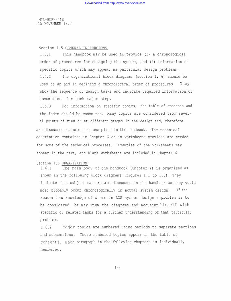
1.5.1 This handbook may be used to provide (1) a chronological
order of procedures for designing the system, and (2) information on
specific topics which may appear as particular design problems.
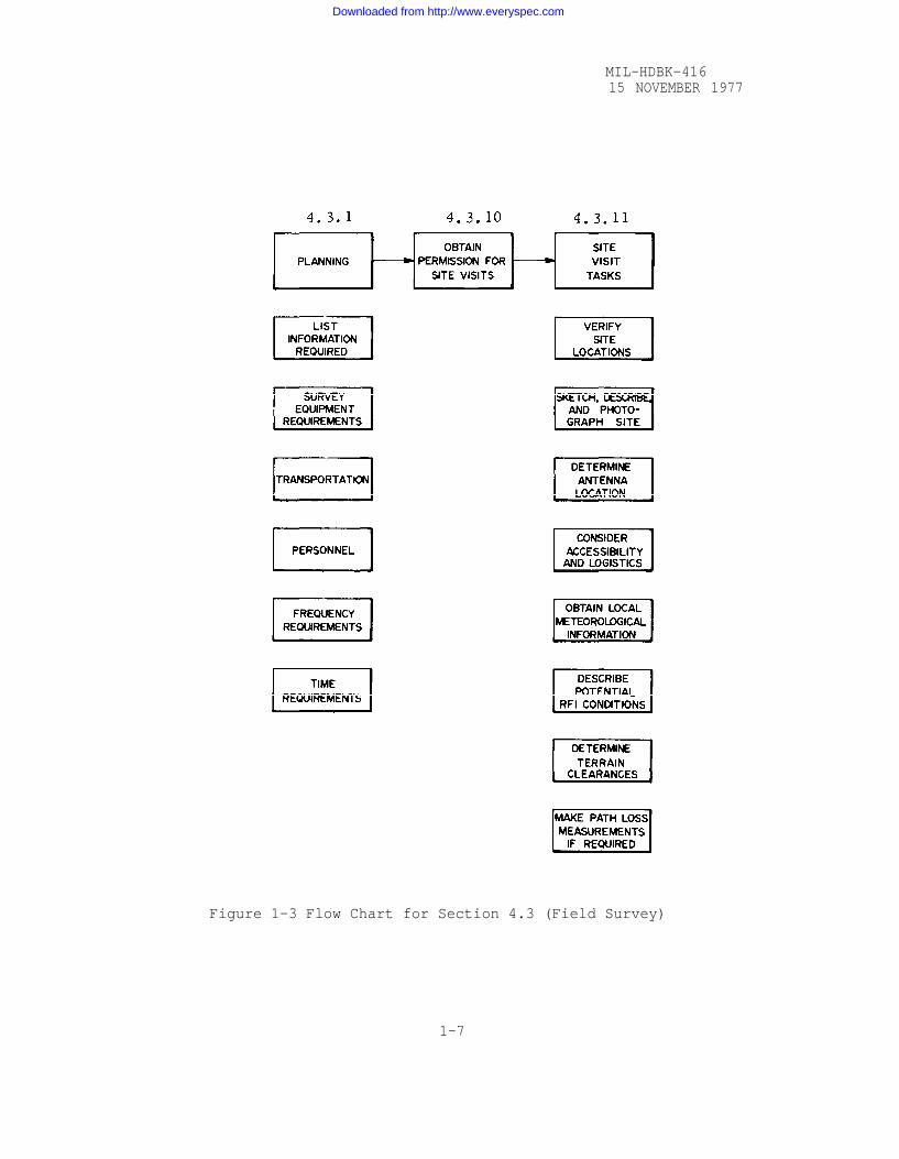
1.5.2 The organizational block diagrams (section 1. 6) should be
used as an aid in defining a chronological order of procedures. They
show the sequence of design tasks and indicate required information or
assumptions for each major step.
1.5.3 For information on specific topics, the table of contents and
the index should be consulted. Many topics are considered from sever-
al points of view or at different stages in the design and, therefore,
are discussed at more than one place in the handbook. The technical
description contained in Chapter 6 or in worksheets provided are needed
for some of the technical processes. Examples of the worksheets may
appear in the text, and blank
Section 1.6 ORGANIZATION.1.6.1 The main body of
worksheets are included in Chapter 6.
the handbook (Chapter 4) is organized
shown in the following block diagrams (figures 1.1 to 1.5). They
indicate that subject matters are discussed in the handbook as they
as
would
most probably occur chronologically in actual system design. If the
reader has knowledge of where in LOS system design a
be considered, he may view the diagrams and acquaint
specific or related tasks for a further understanding of
problem.
1.6.2 Major
and subsections.
contents. Each
numbered.
problem is to
himself with
that particular
topics are numbered using periods to separate sections
These numbered topics appear in the table of
paragraph in the following chapters is individually
1-4
Downloaded from http://www.everyspec.com

Figure 1-1
MIL-HDBK-41615 NOVEMBER 1977
1-5
Downloaded from http://www.everyspec.com

MIL-HDBK-41615 NOVEMBER 1977
1-6
Downloaded from http://www.everyspec.com
MIL-HDBK-41615 NOVEMBER 1977
Figure 1-3 Flow Chart for Section 4.3 (Field Survey)
1-7
Downloaded from http://www.everyspec.com

Figure 1-4
MIL-HDBK-41615 NOVEMBER 1977
1-8
Downloaded from http://www.everyspec.com

MIL-HDBK-416
15 NOVEMBER 1977
1-9
Downloaded from http://www.everyspec.com

This page is blank
1-10
Downloaded from http://www.everyspec.com

MIL-HDBK-41615 NOVEMBER 1977
CHAPTER 2
REFERENCED DOCUMENTS
2.1 Military Standards.
MIL-STD-188 Military Communication System
Technical Standards (to be
replaced by MIL-STD-200 series)
MIL-STD-188-100
MIL-STD-188-300
MIL-STD-188-311
MIL-STD-188-313
MIL-STD-188-340
Common Long Haul and Tactical
Communication System Technical
Standards
Subsystem Design and Engineering
Standards for Technical Control
Facilities
Technical Design Standards for
Frequency Division Multiplexer
Subsystem Design and Engineering
Standards and Equipment Technical
Design Standards for Long-Haul
Communcations Transversing
Microwave LOS Radio and Tropo-
spheric Scatter Radio
Long Haul Communications Standards
Equipment Technical Design Standards
for Voice Orderwire Multiplex
2-1
Downloaded from http://www.everyspec.com

MIL-HDBK-41615 NOVEMBER 1977
MIL-STD-188-342
MIL-STD-188-346
MIL-STD-188-347
MIL-STD-461
MIL-STD-462
MIL-STD-463
MIL-STD-633
Standards for Long Haul Commun-
cations Equipment Technical Design
Stanards for Voice Frequency
Carrier Telegraph (FSK)
Standards for Long Haul Communica-
tions, Equipment Technical Design
Standards for Analog End Instru-
ments and Central Office Ancillary
Devices
Standards for Long-Haul Communica-
tions Equipment Technical Design
Standards for Digital End Instru-
ments and Ancillary Devices
Electromagnetic Interference Charac-
teristics Requirements for Equipment
Electromagnetic Interference Chara-
teristics, Measurement of
Definitions and Systems of Units,
Electromagnetic Interference Tech-
nology
Mobile Electric Power Engine Gener-
ator Standard Family characteristics
Data Sheets
2-2
Downloaded from http://www.everyspec.com

MIL-HDBK-41615 NOVEMBER 1977
MIL-STD-1327 Flanges, Coaxial and Waveguide;
and Coupling Assemblies, Selection of
MIL-STD-1328 Couplers, Directioal (Coaxial Line,
Waveguide, and Printed Circuit)
Selection 01
MIL-STD-1358 Waveguides, Rectangular, Ridged and
Circular, Selection of
MIL-STD-1381 Technical Electronic Terms and
Definitions
2.2 Military Handbooks.
(c) MIL-HDBK-232 Red/Black Engineering-Installation
Guidelines (U)
MIL-HDBK-411 Long Haul Communications (DCS)
Power and Environmental Control
for Physical Plant
MIL-HDBK-417 Facility Design for Tropospheric
Scatter
2.3 Other Referenced Documents.
1. International Telephone and Telegraph Corporation (1970), Refer-ence Data for Radio Engineers, H. P. Westman, ed.,5th edition)Howard W. Sams and Co., New York, N.Y.).
2. STRATCOM (1965), Telecommunications Engineering-InstallationPractices, CCTM-105-5O-3, US Army Communications-Electronics Engineering Installation Agency, ATTN:ACCC-CED-SPT, Fort Huachuca, AZ85613
3. Brodhage, H., and W. Hormuth (1968), Planning and Engineeringof Radio Relay Links, 7th edition (Siemen Aktienge-sellschaft, Munich, Germany).
—
2-3
—
Downloaded from http://www.everyspec.com

MIL-HDBK-41615 NOVEMBER 1977
4. Lenkurt Electric Company (1970), Engineering Considerations forMicrowave Communications System, (GTE LenkurtDept. C134, San Carlos, Calif., 94070).
5. Martin, J. (1969), Telecommunications and the Computer(Prentice-Hall, Englewood Cliffs, N.J.).
6. Hamsher, D.H.,ed. (1967), Communication System EngineeringHandbook (McGraw-Hill, New York, N.Y.).
7. CCIR (1970), Propagation in Non-ionized Media, Xllth PlenaryAssembly, Vol.ll,Part 1 (International TelecommunicationUnion, Geneva, Switzerland).
8. Rice, P.L., A.G. Longley, K.A. Norton, and A.P. Barsis (1967),Transmission Loss Predictions for TroposphericCommunication Circuits, National Bureau of StandardsTechnical Note 101 (Revised), Vol. 1 and 11 (Ntis,1AD 687 820 and AD 687 821).
9. AFCS (1970), Systems Approach to Wideband Communications,AFCSP 100-35 Air Force Communications Service,Scott AFB IL 62225).
10. AFLC (1975), Microwave Relay Systems, AFTO 31r5-1-9(Air Force Logistics Command, OCAMA,Tinker AFB, OKLA).
11. Headquarters, Department of the Army (1965), Map Reading,FM 21-26 (GPO2).
12. CCIR, CCITT (1969), Economic and Technical Aspects of theChoice of Transmission Systems (International Telecom-munications Union, Geneva, Switzerland).
13. Saad, T.S., ed. (1971), Microwave Engineerst Handbook, Vol.Iand II (Aetech House, Inc., Dedham, Mass.).
14. Lenkurt Electric Company (1966), Selected Articles from TheLenkurt Demodulator (GTE Lenkurt Dept. C134),San Carlos, Calif. 94070).
15. Bell Telephone Laboratories (1970), Transmission System for
16. Hogg,D.C.
17. Kerr,D.E.
Communications (Western Electric Company; Inc.,Winston-Salem, N.C.).
(1969), Statistics on Attenuation of Microwaves byIntense Rain, Bell System Tech. J. 48, NO.8, 2949-2962.
ed. (1964), Propagation of Short Radio Waves, Vol. 13,M.I.T. Radiation Laboratory Series (Boston TechnicalPublishers, Inc., Lexington, Mass.).
2-4
Downloaded from http://www.everyspec.com
MIL-HDBK-41615 NOVEMBER 1977
18.
19.
20.
21.
22.
23.
24.
25.
26.
27.
28.
IEEE (1965), Test Procedure for Antennas (Institute of Electricaland Electronics Engineers, New York, N.Y.).
Skerjanec, R.E., and C.A. Samson (1970), Rain Attenuation Studyfor 15 GHz Relay Design, Federal Aviation Adminstra-tion Report FAA-RD-70-21 (NTIS,1 AD (09 348, 1970.
Ryde, J.W., and D. Ryde (1965), Attenuation Of Centimetre andMillimetre Waves by Rain, Hail, Fogs, and Clouds,Rept. 8670 (General Electric Company ResearchLaboratories, Wemble, England).
Brooks, C.E.P., and N. Carruthers (1.946), The Distribution ofHeavy Rain in One and Two Hours, Water and WaterEngineering 49, 275.
Critchfield, H.J. (1960), General Climatology (Prentice-Hall,)Inc., Englewood, N.J. .
Kendrew, W.G. (1963), The Climates of the Continents (OxfordUniversity Press, London, England).
CCIR (1971), Report of the Special Joint Meeting, Part II annexes(International Telecommunications Union, Geneva,Switzerland).
WMO (1956), World Distribution of Thunderstorm Days, Rept. 21(World Meteorological Organization, Geneva, Switzerland ).
U.S. Weather Bureau (1955), Rainfall-Intensity-Duration-Frequency Curves, Tech. Paper 25 (GP02).
Environmental Data Service (1969), Climates 01’ the World (GP02).
Fritschen, L.J., and P.R. Nixon (1967), Microclimate Before
29. Medhurst,
30. Hathaway,
.and After Irrigation, Symposium on Ground LevelMeteorology, Publication No. 86 (American Associationfor Advancement of Science, Washington, D.C.).
R.G. (1965), Rainfall Attenuation of Centimetre Wave:Comparison of Theory and Measurement, IEEE Trans.Ant. prop. AP-13, No. 4, 550-564.
SOD., and H.W. Evans (1959), Radio Attenuation at11 kmc and Some Implications Affecting Relay SystemEngineering, Bell System Tech. J. , No. 1,73-97.
31. Geiger, R. (1965), The Climate near the Ground, (HarvardUniversity Press, Cambridge, Mass.).
2-5
Downloaded from http://www.everyspec.com
MIL-HDBK-41615 NOVEMBER 1977
32. Topil, A. G.(1971), Summer Shower Probability in Colorado asRelated to Altitude, NOAA Tech. Memo. CR-43(NTIS,l COM-71-00712, 1971).
33. Barsis, A.P.,K.A. Norton, and P.L. Rice (1962), Predicting thePerformance of Tropospheric Links, Singly and inTandem, IRE Trans. Commun. Systems CS-10, No. 1, 2-22
34. Hogg, D.C.(1968), Millimeter-Wave Communication through theAtmosphere, Science 159, No. 3810, 39-46.
35. Dougherty, H.T. (1968), A Survey of Microwave Fading Mecha-nisms, Remedies and Applications, ESSA Tech. Rept.ERL 69-WPL 4 (NTIS,l COM-17-50288).
36. Albertson, J.N. (1964), Space Diversity on the Microwave Systemof the Southern Pacific Co., Wire and Radio Commun.No. 11, 83-87.
37. Bateman, R. (1946), Elimination of Interference-Type Fading atMicrowave Frequencies with Spaced Antennas, Proc.IRE 34, No. 5, 662-676.
38. Bean, B.R., and E.J. Dutton (1966), Radio Meteorology, NBSMonograph 92 (GP02).
39. Bean, B. R., B.A. Cahoon, C.A. Samson, and G.D. Thayer (1966),A World Atlas of Atmospheric Radio Refractivity, ESSAMonograph 1 (GP02).
40. Beckmann,
41. Beckmann,
P. (1962), Statistical distribution of the amplitude andphase of multiply-scattered field, J. Res. NBS Radioprop. 66D, NO. 3, 231-240.
P., and A. Spizzichino (1963), The Scattering ofElectromagnetic Waves from Rough Surfaces, Inter-national Series of Monographs on ElectromagneticWaves, Vol. 4 (Pergamon Press, New York, N.Y.).
42. Beckmann, P. (1964), Rayleigh distribution and its generalizations,Radio Science, J. Res. NBS 68D, Noe9, 927-9320
43. Brekhovskikh, L. (1960), Wave in Layered Media (AcademicPress, New York, N.Y.).
44. Burns, W.R. (1964), Some statistical parameters related to theNakagami-Rice probability distribution, Radio Science,J. Res. NBS 68D, No. 4, 429-434.
45. Burrows, C.R., and S.S. ATTwood (1949), Radio Wave Propagation(Academic Press, New York, N.Y. ).
2-6
Downloaded from http://www.everyspec.com
MIL-HDBK-41615 NOVEMBER 1977
46. Bussey, H.E. (1950), Reflected ray suppression, Proc. IRE 38,No. 12, 1453.
47. Cabessa, R. (1955), The achievement of reliable radio communica-tion links over maritime paths in Greece (in French),LfOnde Electrique 35, 714-727.
48. Doherty, L.H. (1952), Geometrical optics and the field at a causticwith applications to radio wave propagation betweenaircraft, Research Rept. EE 138 (Cornell University,Itaca, New York, N.Y.).
49. Dougherty, H.T., and R.E. Wilkerson (1967), Determination ofantenna height for protection against microwave diffrac-tion fading, Radio Science 2, No.2, (New Series), 161-165.
50. Dougherty, H.T. (1967), Microwave fading with airborne terminals,ESSA Tech. Rept. IER 58-ITSA 55 (GPO2).
51. White, R.F. (1968), Space diversity on line-of-sight microwavesystems, IEEE Trans. Commun. Technol. Com-No. 1, 119-133.
52. DuCastel, F., P. Miame, and J. Voge (1960), Sur le role desphenomenes de reflexion clans la propagation lointainedes ondes ultracortes, Electromagnetic Wave Propaga-tion (Academic Press, New York, N.Y.)., 670-683.
53. Furutus, K. (196>), On the field strength over a concave sphericalearth, (unpublished ITS study).
Hogg, D.C. (1967), Path diversity in propagation of millimetercurves through rain, IEEE Trans. Ant. Prop. AP-15,No, 3, 410-415.
Hoyt, R.W. (1947), Probability functions for the modulus and angleof the normal complex variety, Bell System Tech.J. 26, 318-359.
Hufford, G.A. (1952), An integeral equation approach to the problemof wave propagation over an irregular surface, Quart.Appl. Math. 9, No. 4, 391-404.
57. Katzin, M.R., W. Bachman, and W. Binnian (1947), Three andnine centimeter propagation in low ocean ducts} Proc.IRE 35, No. 9, 831-905.
58. Kawazu, S., S. Koto, and K. Moriata (1959), Over-sea propaga-
tion of microwave and anti-reflected-wave antenna,Reports of ECL (Japan) 7, 171-191.
2-7
Downloaded from http://www.everyspec.com

MIL-HDBK-41615 NOVEMBER 1977
59. Lewin, L. (1962), Diversity reception and automatic phase correc-tion, Proc. IEE, Part B, 109, 295-304.
60. Magnuski, H. (1956), An explanation of microwave fading and itscorrection by frequency diversity, presented at theAIEE, Winter General Meeting in New York, N.Y. ,56-376.
61. Makino, H., and K. Morita (1967), Design of space diversityreceiving and transmitting systems for line-of-sightmicrowave links, IEEE Trans. Commun. SystemsCOM-15, No. 4, 603-614.
62. Matsuo, S., S. Ugai, K. Kakito, F. Ikegami, and Y. Kono (1953),Microwave fading, Reports of ECL (Japan) 1, No. 3,38-47.
63. Murray, J.W., and H.M. Flager (1965), Improving microwavesystem reliability, First IEEE Annual Commun. Con-vention Conference Record, 245-248.
64. Moreland, W.B. (1965), Estimating meteorological effects onradar propagation, Air Weather Service TechnicalReport No. 183, 1, 45, 143.
65. Nakagami, M. (1943), Statistical characteristics of short wavefading, J. Inst. Elec. Commun. Engr. (Japan).
66. Nakagami, M. (1964), On the intensity distributions and its appli-cation to signal statistics, Radio Science, J. Res. NBS68D, No. 9, 995-1003.
67. Norton, K.A., L.E. Vogler, W.V. Mansfield, and P.J. Short(1955), The probability distribution of the amplitudeof a constant vector plus a Rayleigh-distributedvector, Proc. IRE 43, No. 10, 1354-1361.
68. Norton, K.A., G.A. Hufford, H.T. Dougherty, and R.E. Wilkerson(1965), Diversity design for within-the-horizon radiorelay system, Informal NBS Rept 8787 (Institute forTelecommunication Sciences, Boulder, Colo. 80302).
69. Preikschat, F.K. (1964), Screening fences for ground reflectionreduction, Microwave J. 7, No. 8, 46-50.
70. Quarta, P. (1966), Propagation tests on an oversea path (Mt.Verrugoli-Mt. Portofino), Alta Frequenza 35, No. 5,364-369 (in English).
71. Rice, S.0. (1944, 1945), Mathematical analysis of random noise,Bell System Tech. J. 23, 282-332; 24, 46-156.
2-8
Downloaded from http://www.everyspec.com

72.
73.
74.
75.
76.
77.
78.
79.
80.
81.
82.
83.
84.
MIL-HDBK-41615 NOVEMBER 1977
Sharpless, W.M. (1946), Measurement of the angle of arrival ofmicrowaves, Proc. IRE 34, No. 11, 837-845.
Smith, E.K., and S. Weintraub (1953), The constants in theequation for atmospheric refractive index at radiofrequencies, Proc. IRE 41, No. 8, 1035-1037.
Ugai, S., S. Aoyagi, and S. Nakahara (1963), Microwave trans-mission across a mountain by using diffractor gratings(in Japanese), J. Inst. Elec. Commun. Engr. (Japan)46_, 653-661.
Vigants, A. (1968), Space-diversity performance as a function ofantenna separation, IEEE Trans. Commun. SystemsCOM-16, No. 6, 831-836.
Wait, J.R. (1962), Electromagnetic Waves in Stratified Media,International Series on Monographs on ElectromagneticWaves, Vol. 3 (Pergamon Press, New York, N.Y.).
CCIR and CCITT (1971), Propagation, Appendix to Section B.iv.3of the Handbook Economic and Technical Aspects of theChoice of Transmission Systems (International Tele-communications Union, Geneva, Switzerland).
Turner, D., B.J. Easterbrook, and J.E. Gelding (1966), Experi-mental investigation into radio propagation at 11 .0-11.5Gc/s, Proc. IEE (Br) 113, No. 9, 1477-1489.
Polyzou, J., and M. Sassier (1960), Path loss measuring techniquesand equipment, IRE Trans. Commun. Systems 9-13.
Medhurst, R.G. (1959), Echo Distortion in Frequency Modulation,Electronic and Radio Engineer 36, July, 253-259.
CCIR (1970), Fixed Service Using Radio-Relay Systems (StudyGroup 9). Coordination and Frequency Sharing BetweenCommunication-Satellite Systems and TerrestrialRadio-Relay Systems (Subjects Common to Study Groups4 and 9), XIIth Plenary Assembly, Vol. IV, Part I(International Telecommunications Union, Geneva,Switzerland).
Brennan, D.G. (1959), Linear Diversity Combining Techniques,proc. IRE 47, No. 6, 1075-1102.
Barnett, W.T. (1972), Multipath Propagation at 4, 6 and 11 GHz,Bell System Tech. J. 51, No. 2.
Crawford, A.B., and W.C. Jakes (1952), Selective fading ofmicrowaves, Bell System Tech. J. 31, 68-90.
2-9
Downloaded from http://www.everyspec.com

MIL-HDBK-41615 NOVEMBER 1977
85. Nomura, et al, (1967), Distortion due to fading in high-capacityFDM-FM transmission, Electronic and Electrical Communica-tions (Japan) Vol. 50, No. 6.
86. Giugliarelli, G. (1965), On the influence of oversea propagation onthe transmission of colour television signals, E.B.U.Review, 90-A, Technical.
87. Takada, M., S. Kate, S. Ito, and S. Nakamura (1968), SF-F2short-haul radio relay system in the 15 GHz Band,Review of the Elec. Commun. Lab., N.T.T., 16,No. 7-8, 613-641.
88. Fehlhaber, L., and J. Grosskopf (1965), Contribution to theexplanation of fading phenomena on line-of-sight radiolinks in the decimetric and centrimetric bands,Technischer Bericht No. 5578, FernmeldetechnischesZentralamt.
89. Smith, Rose, R.L., and A.C. Stickland (1946), An experimentalstudy of the effect of meteorological conditions uponthe propagation of centimetre radio waves, MeteorologicalFactors in Radio Wave Propagation, Physical Sot. ofLondon.
90. Bureau of Land Management (1972), The Ephemeris, prepared bythe Nautical Almanac Office, U.S. Naval Observatory(Supt. of Documents, GP02).
91. K & E (1971), The 1972 Solar Ephemeris and Surveying Instru-ment Manual (Keuffel and Esser Co., Morristown, N.J.).
92. U.S. Weather Bureau (1963), Manual of Barometry, Vol. 1, 2-792to 2-103 (Supt. of Documents, GPO ).
93. Sharp, H.O., and R.K. Palmer (1948), Faster and cheaper fieldsurveys, Engineering News-Record 141, 75-78.
94. Cassie. W.F., ed. (1956), A treatise on Surveying (Middleton &Chadwick’s), Vol. 2, 331-338, revised 6th ed.(Philosophical Library, New York).
95. Bureau of Land Management (1947), Manual of Instructions for theSurvey of the Public Lands of the U.S. (Supt. of
2Documents, GPO , 1968 reprint).
96. Rayner, W.H., and M.O. Schmidt (1957), Surveying (D. Van Nostrandco. , Princeton, N.J.).
97. Skerjanec, R.E., and C.A. Samson (1972), Microwave link performancemeasurements at 8 and 14 GHz, DOT/FAA ReportFAA-RD-72-115 (NTIS, 1 AD-756 605)0
2-10
Downloaded from http://www.everyspec.com

MIL-HDBK-41615 NOVEMBER 1977
98. DCA (1968), DCS engineering-installation standards manual,Defense Communications. Agency Circular 330-175-1(Director DCA, ATT: Code 212, Washington, DC 20305).
99. ITU (1957), Radio Regulations, (International TelecommunicationUnion, Geneva, Switzerland).
100. Samson, C.A. (1975), Refractivity gradients in the northernhemisphere, Office of Telecommunications ReportOT 75-59 (Supt. of Documents, GP02).
101. Vogler, L.E. (1964), Calculation of groundwave attenuation inthe far diffraction region, J. Res. NBS, 68D (Radioscience), No. 7, 819-826.
102. Norton, K.A., P.L. Rice, and L.E. Vogler (1955), The use of
103. Nishikoro,
angular distance in estimating transmission loss andfading range for propagation through a turbulentatmosphere over irregular terrain, Proc. IRE 43,No. 10, 1488-1526.
K ., Y. Kurihara, M. Fukushima, and M. Ikeda (1957),Broad and narrow beam investigations of- SHF diffractionby mountain ridges, J. Radio Res. Labs. (Japan), 4,No. 118, 407-422.
104. Boithias, L., and J. Battesti (1967), Protection against fadingon line-of-sight radio relay systems (in French),Annales des Telecommunications, 22, No. 9-10, 230-242.
105. DCA (1971), Site Survey Data Book for Communications Facilities,DCA Circular 370-160-3 (Director DCA, ATT: Code 212Washington, D.C. 20305).
106. DOT (1973), Obstruction Marking and Lighting, AC 70/7460-lC(Department of Transportation, Distribution Unit,TAD-484.3, Washington, D.C. 20590).
107. ASHRAE American Society of Heating, Refrigeration and Air-Conditioning Engineers Guide and Data Book (AmericanSociety of Heating, Refrigerating and Air-ConditioningEngineers, Inc. 345 E. 47th Street, New York, NY 10017).
108. TM5-785, NAFAC P-89, AFM 88-8 Individual service manuals ofArmy, Navy and Air Force containing EngineeringWeather Data.
1 Copies of these reports are sold by the National Technical InformationService, Operations Division, Springfield, VA 22151. Order by indicatedaccession number.
2 Copies of these reports are sold by the Superintendent of Documents,U.S. Government Printing Office, Washington, D.C. 20402.
2-11
Downloaded from http://www.everyspec.com

This page is blank
Downloaded from http://www.everyspec.com

CHAPTER 3.0MIL-HDBK-41615 NOVEMBER 1977
3.0 TERMS AND DEFINITIONS (MIL-STD 188-120)
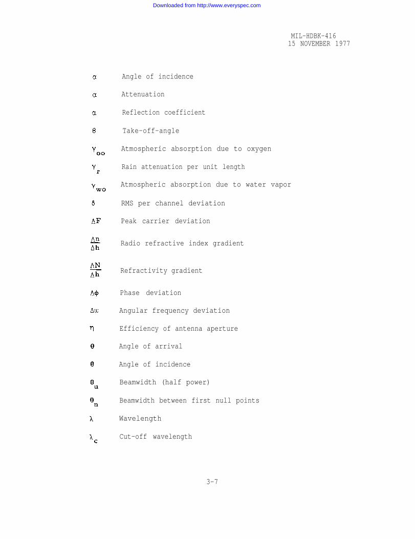
3.1 Symbols
A
A
A
a
A a
A c
A f
A i
A r
Atl
b
b
B b
B c
bc
B o
brf
C
C
Area
FParameter A or
Total attenuation attributable to atmospheric andterrain effects
Terrain factor
Atmospheric absorption
Circulator loss
Transmit forward feeder attenuation
Isolator loss
Transmit reverse feeder attenuation
Transmission line loss
Bandwidth
Climate factor
Baseband bandwidth
Bandwidth of the RF channels
Usable voice channel bandwidth
Receiver IF bandwidth
Mid frequency separation
RF bandwidth
Velocity of light
RF carrier level
3-1
f m
BIF
Downloaded from http://www.everyspec.com

MIL-HDBK-41615 NOVEMBER 1977
C/N
C r
D
D
d
d
d n
d s
E
ERP
es
F
f
F a m
f m
F n
G
G
G p
Carrier-to-noise ratio
Fresnel zone clearance
Antenna diameter
Maximum dimension of an antenna aperture
Great circle path distance
A side dimension of a reflector
Nominal path length
Lateral separation of route diversity paths
Electric field
Effective radiated power
Saturation vapor pressure
Receiver noise figure
Frequency
Median operating noise factor
Lowest frequency in the baseband
Maximum modulating frequency
nth Fresnel zone
Geometric mean of the transmitting andreceiving antenna power gains
Antenna gain above isotropic
Gain of the projected aperture of a passiverepeater
3-2
f
Downloaded from http://www.everyspec.com

MIL-HDBK-41615 NOVEMBER 1977
H
h
hs
Id
Ip
K
k
k
k TBF
L
L b f
LF
lf
L o f
L p
Lt
M F
M f
N
Height
Vertical distance
Average height of the two, path terminalsabove msl
Diversity improvement
Pre-emphasis improvement
K is a measure of the anisotropic scatteringof the random components by the terrain
Ratio of effective earth’s radius to actualearth radius, or the equivalent earth’sradius factor
Boltzman’s constant,1.3804 X 10-20 millijoules/0K
Receiver noise threshold
Transmission loss
Basic free-space transmission loss
RMS load factor
Numerical RMS load factor
Free-space path l0SS
Median value of power loss between antennaterminals on a passive repeater link
Transmission line length (transmitter)
Fading depth exceeded below free space
Fade margin
N = (n-1) 106 (refractivity)
3-3
Downloaded from http://www.everyspec.com

MIL-HDBK-41615 NOVEMBER 1977
N
n
n
N e
NF
N f
N i m
NPR
N s
N t
N t e
N T m e d
N T T H
N t T H
Number of channels
Radio refractive index
Number of equivalent voice channels
Equipment intermodulation noise
Noise figure
Feeder echo noise
Total path independent non-linear noise
Noise power ratio
Surface refractivity
Thermal noise
Emphasis - improved thermal noise
Total median noise
Total noise at FM threshold
Emphasis - improved thermal noise at threshold
Diversity and emphasis - improved thermalnoise at threshold
P Pressure
P eProbability of error
PF Peak factor
pf Numerical peak factor
P m fPercent of year that fades exceed a specifieddepth below free-space loss
P r Received RF signal level
3-4
NtTH(E,D)
Downloaded from http://www.everyspec.com

MIL-HDBK-41615 NOVEMBER 1977
P r T H Received signal level at FM threshold
Pt Transmitter power
Distancer
Echo amplituder
Radius of curvature of the radio rayr
Signal levelr
rms value of the signal level
R Reliability
Relative humidity in percentR H
Transmit return lossR Lt
nth Fresnel zone radius
Radius of the earth (rO 6370 km)
R n
ro
Rainfall rateR r
S Signal level
S The RMS Rayleigh signal level in decibelsabove the RMS multipath,
S/D
T
Signal-to-distortion ratio
Temperature (°K)
Velocity of propagationv
V
VSWR
Voltage
Voltage standing wave ratio
3-5
Downloaded from http://www.everyspec.com

MIL-HDBK-41615 NOVEMBER 1977
Z
Z
Z = 20 log10
Impedance
3-6
Downloaded from http://www.everyspec.com
MIL-HDBK-41615 NOVEMBER 1977
Angle of incidence
Attenuation
Reflection coefficient
Take-off-angle
Atmospheric absorption due to oxygen
Rain attenuation per unit length
Atmospheric absorption due to water vapor
RMS per channel deviation
Peak carrier deviation
Radio refractive index gradient
Refractivity gradient
Phase deviation
Angular frequency deviation
Efficiency of antenna aperture
Angle of arrival
Angle of incidence
Beamwidth (half power)
Beamwidth between first null points
Wavelength
Cut-off wavelength
3-7
Downloaded from http://www.everyspec.com

MIL-HDBK-41615 NOVEMBER 1977
Sum of reflection coefficient magnitudes
Reflection coefficient
Standard deviation of the heights of surfaceirregularities
Echo delay time
Incident angle of the reflected ray
Baseband angular frequency
3-8
Downloaded from http://www.everyspec.com

CHAPTER 4
SYSTEM DESIGN
Section 4.0 INTRODUCTION.
4.0.1 Chapter 4 contains information necessary for designing the
line-of-sight microwave system with the exception of facility design
criteria such as detailed information on physical plant layout, primary
power, tower and antenna structure, safety, etc. , which is presented
in Chapter 5.
4.0.2 Section 4.1 discusses gathering information on functional
requirements and resource limitations; it also discusses the content of
the engineering implementation plan which must be prepared as the
design effort proceeds. Section 4.2 describes a systematic approach to
the selection of sites and routes which tends to grade them in such a
way as to prevent good candidate paths from being overlooked or elimin-
ated. On the basis of grading described in section 4.2, certain paths
and sites are selected for additional investigation by field survey.
Field survey techniques and requirements are considered in section
4.3. Information on
detailed link design,
conditions, potential
path profiles and site conditions is used in the
section 4.4. Path geometry, local meteorological
interference sources, and basic microwave equip-
ment are involved. Section 4.5 takes up the problem of integrating the
links into a compatible system. This task includes system layout,
frequency allocation, intra-system interference and the preparation of
system performance predictions. Chapter 4 is organized as shown in
the flow diagrams of section 1.6.
4.0.3 Quantative information on the topics described above is
contained throughout the various sections of Chapter 4. This informa-
tion is contained primarily in the form of graphs and tables for ease of
application. Several equations, however, were considered necessary.
4-1
MIL-HDBK-41615 NOVEMBER 1977
Downloaded from http://www.everyspec.com

MIL-HDBK-41615 NOVEMBER 1977
Units and definitions of terms are supplied in the immediate context of
the equations. In cases where descriptive material describing the same
topic appears in more than one place in the text, we have attempted to
supply suitable cross-referencing.
4-2
Downloaded from http://www.everyspec.com

MIL-HDBK-41615 NOVEMBER 1977
4.1
4.1.1
4.1.1.1
copies
STARTING THE DESIGN
General
At the start of LOS microwave system design, several
of an outline map of the general area to be served should be
obtained. An example of such a map is shown later on in figure 4.5-1.
One or more of these maps can be used to record information relevant
to the system as it becomes available. These outline maps can also be
made to serve as an index to more detailed information about the
system, e. g., an approximate grid of suitable larger-scale maps can
be drawn on the outline map, and site designations can be shown at
their approximate location with more detailed information provided in
tabular form. Information on functional requirements (sec. 4.1.2)
and resource limitations (sec. 4.1.4) should be collected, and organized
to start the Engineering Implementation Plan (sec. 4.1.12) and
analyzed to determine basic feasibility (sec. 4.1.14).
4.1.2 Functional Requirements
4.1.2.1 The functional information about the system that must be
obtained includes channel types (quantities and quality), terminal
locations, direction of information flow, compatibility with existing
equipment and services, and flexibility for expansion. Uncertainty in
functional requirements often translate into additional system costs
because increased flexibility must be designed into the system.
Although flexibility is very desirable if it can be obtained at little cost,
it is often very costly in available resources and can be obtained only
at the expense of other valuable features.
4.1.2.2 Communication centers that are to be connected through
the main trunk should be located as precisely as possible. Radio
4-3
Downloaded from http://www.everyspec.com

terminals that are to be serviced by spur links off the main trunk
should also be located. The positions of radio terminals help to outline
a large strip of terrain that is desirable for locating the main trunk.
Information about the channel types, capacity, quality, quantities, and
direction of flow is necessary for determining spectrum and power
requirements.
4.1.2.3 Plans or possibilities for future system expansion should
be examined. Appropriate planning for the initial system must include
provisions for later upgrading or expansion so that site reconfiguration
or new construction can be minimized. The designer should also
consider future channel requirements in addition to current needs when
specifying equipment. System upgrading may necessitate enlargement
of buildings, greater air conditioning capacity, increased logistic
capabilities, enlargement of the siting area, and possibly relocation of
existing stations, or addition of new terminal or repeater sites.
4.1.3 Channel Parameters
4.1.3.1 Information on the number and quality of channels, required
bandwidth, and direction of traffic flow is needed to determine frequency
spectrum and power requirements. Such information for FDM-FM
systems can be listed using the format in Worksheet 4.1-1 for each
link. It provides also the basis for estimating spectrum requirements
for the purpose of requesting frequency assignments (see sec. 4.1.10).
4.1.3.2 Nominal values given in Worksheet 4.1-1 may be used in
lieu of more current information. The relation between the number of
voice channels, per-channel deviation, and the total radio frequency
spectrum requirements is shown in figure 4.1-1, and will also be
discussed later on in section 4.5.5. The number of channels needed
to carry traffic over each link will often be equal in both directions.
4-4
MIL-HDBK-41615 NOVEMBER 1977
Downloaded from http://www.everyspec.com

MIL-HDBK-41615 NOVEMBER 1977
Current and future channel requirements for traffic
from site to site .
NumberType of ofChannel Channels
Voice(Telephone)Voice(Facsimile)Voice(Low Speed Data)Voice(Medium Speed Data)Digital Data(High Speed)
Video
Basebandper
Channel Qualitv
Equivalentvoice chan-nels per infor-mation channel
Totals
Link channel requirements
rounded to the next highernominal value 1
Number ofequivalentvoice Basebandchannels Spectrum
Transmitter RF bandwidth2
(Future Expansion)Voice(Telephone)Voice(Facsimile)Voice(low Speed Data)Voice(Medium Speed Data)Digital Data(High Speed)Video
1 Nominal values are 24, 60, 120, 300, 600, 960, and 1800.2 Estimate using figure 4.1-1.
Worksheet 4.1-1 Format for Recording Channel Requirements for FDM-FM Systems.
4-5
Downloaded from http://www.everyspec.com

MIL-HDBK-41615 NOVEMBER 1977
4-6
Downloaded from http://www.everyspec.com

MIL-HDBK-41615 NOVEMBER 1977
The total spectrum requirements may, however, be double the values
determined here if it is necessary to employ frequency diversity.
This may have to be considered when extremely long or otherwise
difficult links are involved, but cannot really be determined until the
procedures in section 4.2 have been followed through.
4.1.3.3 Similarly, transmitter power requirements must also
await the results of preliminary design calculations. However, in the
case of LOS systems the required transmitter power values will seldom
exceed 10 watts, and this value may be used at least initially in the
application for frequency assignment.
4.1.4 Resource Limitations
4.1.4.1 Resource limitations must be studied to determine costs
and feasibility. These limitations include economic restraints, real
estate availability, construction limitations, spectrum availability,
socio-political considerations (especially in foreign countries), and
time. Information (even for the initial input) should be as complete,
comprehensive, and accurate as possible. Known major resource
limitations should be compiled, and a list should also be made of
potential major limitations for which the information resulting from
initial surveys is inadequate. Systematic methods should be set up to
seek and utilize additional information on resource limitations as
system design proceeds.
4.1.5 Economic Restraints
4.1.5.1 The initial system cost estimates are important because
requests for final project funding may be based on these
The design engineer should keep cost estimates updated
proceeds, so that fiscal planners have sufficient time to
requests, if need be. FM/FDM multiplexing equipment
estimates.
as the design
modify funding
costs are
4-7
Downloaded from http://www.everyspec.com

nearly proportional to the number of channels over the path, whereas
for a TDM system much of the circuitry is common and the terminal
costs rise slowly as the channel requirement increases. Terminal
costs for microwave equipment rise only slowly since much circuitry
is common. The cost for diversity equipment, waveguide, towers,
heating and air conditioning, etc. , are relatively fixed and will be
similar at each site. Building costs may vary widely over the area
covered by a specific system, and if construction must be speeded up
to meet an operational deadline, the costs may escalate rapidly because
of premium pay for overtime work.
4.1.6 Real Estate Availability
4.1.6.1 There are usually many factors limiting the number of
suitable terminal and relay sites. Some of these factors are large
bodies of water, blockage by terrain or terrain clutter (without using un-
acceptably high towers), prior use of suitable sites, political bounda-
ries, potential interference with other radio systems, local zoning
regulations ease of access, and environmental aspects. Site availabil-
ity investigations should include a check into possible site security
problems. Particularly, unattended operation increases the possibility
of theft, vandalism, or other damage and may require special and
substantial considerations. Site development costs will generally be
subs tantially lower if a site can be found on government-owned lands,
rather than on private property.
4.1.7 Construction Limitation
4.1.7.1 The most common and important construction limitation
is that of tower height. Towers exceeding a given height may violate
local ordinances for a number of reasons. If a link will be near an
airport, or in established air corridors, the site proposed may not be
4-8
MIL-HDBK-41615 NOVEMBER 1977
Downloaded from http://www.everyspec.com

MIL-HDBK-41615 NOVEMBER 1977
approved if it requires the use of high towers. Similar restrictions
may be encountered in or near residential areas, or in certain scenic
areas. A very remote site may involve special construction restric-
tions if access roads will not permit heavy equipment (e. g., cranes) to
reach the site. Certain types of construction materials may be unavail-
able or unduly expensive in some areas, and special types of construc-
tion may be necessary because of local climatic conditions, as in the
arctic, or extremely wet regions, or in regions subject to earthquakes.
4.1.8 Primary Power Limitations
4.1.8.1 Definite information on the availability of commercial
electric power will probably have to await the results of site surveys.
Initially, it will be sufficient to determine from available reference
sources or contacts in the area of the proposed system whether or not
such power is likely to be available. If power for a site must be pro-
vided by engine-generator sets, the problem of hauling fuel to the site
must be considered, as well as the additional expense involved for
buildings, equipment, fuel storage and even operating personnel if the
equipment cannot be automated. The principal power requirements for
LOS systems will come from heating and cooling demands since trans-
mitter power is usually quite low.
4.1.9 Frequency Spectrum Availability
4.1.9.1 The designer should work through the applicable Frequency
Allocation Office to determine what blocks of frequencies can be made
available for the proposed system. Despite the lack of specific informa-
tion on system parameters and routing, it is important that early
contact be made with this office, since at least a preliminary commit-
ment must be available prior to the feasibility study. The designer
should assemble as much information on the proposed system as
4-9
Downloaded from http://www.everyspec.com

MIL-HDBK-41615 NOVEMBER 1977
possible prior to this initial contact, e. g., the geographical area
involved, approximate locations of terminals or installations to be
served, and probable RF power and bandwidth requirements. At least
general information on the size of antennas and type of terminal
equipment will probably also be available at this time. Further infor-
mation on the type of information generally required for frequency allocations
is given in paragraph 4.1.11.1, but the exact format for a particular case
should be obtained from the Frequency Allocation Office. For extensive
systems, more than one nation may be involved in the frequency alloca-
tion negotiations. This can result in considerable delay in obtaining
the desired assignment, so it is very important that the system designer
work closely with the Frequency Allocation Office from the beginning
of the design effort.
4.1.10 Radio Frequency Assignment
4.1.10.1 Frequency assignments are made through negotiations with
the frequency-controlling agencies of the countries where the system is
to be installed. These negotiations are conducted by the Military
Communications-Electronics Board (MCEB) of the Department of
Defense. In carrying out these negotiations, the MCEB utilizes the
services of portions of certain agencies established for this purpose:
the Frequency Allocation Panel, U.S. (FAPUS); the Frequency Divi-
sion of the Defense Communications System Directorate; the
Communications -Electronics Directorate of the Joint Chiefs of Staff
(J-6); and the Frequency Branches of the Communications-Electronics
Divisions of the Unified Commands. The system engineering function
in this process is to provide the necessary technical inputs for the
negotiations.
4-10
Downloaded from http://www.everyspec.com

MIL-HDBK-41615 NOVEMBER 1977
4.1.11 Application for Frequency Allocation
4.1.11.1 Table 4.1-1 contains a list of items usually specified in
applications for a frequency allocation. Each item of the list that is
pertinent to LOS system planning should be included in the application
if known. (This information was adapted from pp. 4-172 to 4-175 of
[2]).
4.1.12 Engineering Implementation Plan (EIP) Contents and Organization.
4.1.12.1 The EIP is a compiled report of all factors that contribute
toward the development of the microwave radio system, from the
initial proposal to the final system acceptance. It is recommended
that the EIP be started as soon as information on functional require-
ments and resource limitations become known, and will consist of
notes, letters, maps, tables, profiles and sketches, etc. The EIP will
be primarily an organization of known data, and its first use will
contribute toward the completeness and insure the availability of infor-
mation necessary for the determinations that must be made during the
feasibility study. It must be complete and its contents kept timely,
since it will continually be used as a basis for decision and proposal
implementation.
4.1.12.2 All system design data that are developed and used for
decisions should be placed into the EIP. For purposes of determining
required content and organization, it is recommended that the EIP be
organized in accordance with the worksheets supplied in Chapter 6.
This organization separates the EIP material according to individual
sites and links. Because some material is applicable to both sites and
links, appropriate cross referencing should be used. Material which
is applicable to the whole system, such as system layout and frequency
4-11
Downloaded from http://www.everyspec.com

Table 4.1-1
MIL-HDBK-41615 NOVEMBER 1977
4-12
Downloaded from http://www.everyspec.com

Table 4.1-1
MIL-HDBK-41615 NOVEMBER 1977
4-13
Downloaded from http://www.everyspec.com
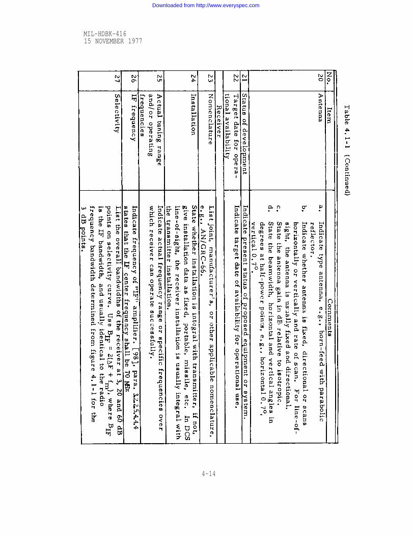
Table 4.1-1
MIL-HDBK-41615 NOVEMBER 1977
4-14
Downloaded from http://www.everyspec.com

Table 4.1-1
15 NOVEMBER 1977
4-15
MIL-HDBK-416
Downloaded from http://www.everyspec.com

plans, must be separated according to individual categories. For
example, all discussions, letters, etc. , pertaining to the availability
of frequency spectrum would be placed in the system EIP under
“Frequency Planning.“
4.1.12.3 Original material should be placed in the EIP as soon as
it is available, and reproduced copies made for discussion or transfer
to other parties. This will soon become quite large, but the designer
is cautioned to save all contributing data and insure that they are
properly cataloged. It may also be desirable to prepare a smaller,
edited system plan that summarizes the design effort and gives only
those details which are of primary importance.
4.3.13 EIP Deadlines and Schedules .
4.1.13.1 Requirements for the design of a system will usually
include one or more deadlines for the completion of various tasks.
Deadlines will have to be considered when planning for procurement of
construction materials, scheduling employment of personnel, and
establishing lead time necessary for sub-contracting, equipment pro-
curement, and related efforts. To insure that planning objectives are
realistic, a table of events for the project should be prepared and made
available for early review. This scheduling may be prepared using a
flow chart or a simple scheduling chart such as the one shown on
table 4.1-2, which is based on one calendar year. More details
in scheduling will be required as the design progresses.
4.1.14 Determine Basic Feasibility
4.1.14.1 During the design phase there are usually two times when
the feasibility of the proposed system may be evaluated. The first is
after completion of the survey of functional requirements and resource
limitations. Final feasibility evaluation should be made prior to
4-16
MIL-HDBK-41615 NOVEMBER 1977
Downloaded from http://www.everyspec.com

Table 4.1-2
MIL-HDBK-41615 NOVEMBER 1977
4-17
Downloaded from http://www.everyspec.com

MIL-HDBK-41615 NOVEMBER 1977
actual site and equipment purchase. This is possible after detailed
studies of expected system performance based on field surveys where
necessary, and of accurate cost data for preparing each site. However,
the design engineer must continuously verify that the limitations
previously investigated with regard to resources do not impose insur-
mountable barriers.
4.1.15 Review Requirements vs. Limitations
4.1.15.1 The engineer should review the information gathered to
insure its completeness so that appropriate authority may later view
and determine the soundness of the system proposal. Based on informa-
tion received, there may be problems and questions requiring solutions
before a decision to continue or not can be made. The design engineer
must also be aware of available alternatives to the design plan. For
instance, if existing LOS links can be incorporated into the design
through upgrading and still fulfill the system requirements, such a
recommendation should be made to the reviewing authority. Finally,
all data for use in determining feasibility should be duplicated for
dissemination to insure that persons involved with the system keep
informed on the current status.
4-18
Downloaded from http://www.everyspec.com

MIL-HDBK-41615 NOVEMBER 1977
Section 4.2 STUDY OF ROUTE ALTERNATIVES.
4.2.1 General
4.2.1.1 If the preliminary assessment of the proposed microwave
system indicates that its requirements might be met within the limita-
tions imposed, a study should be started directed toward selection of
routes and sites.
4.2.1.2 This selection study requires the choosing of preliminary
sites and routes. Drawing profiles and making rough estimates of
path loss probability distributions for each link will help eliminate
potentially troublesome links. This information, along with additional
input such as meteorological data, propagation information from other
links in the immediate area, area radio interference data, etc., should
be evaluated to make a firm selection of primary and alternate routes,
with their associated site locations. For additional information on the
organization of section 4.2, see figure 1-2.
4.2.2 Select Potential Sites
4.2.2.1 Site selection will initially be made considering the use of
available areas and choosing sites on the basis of information obtain-
able from topographic maps. Additional aspects of site choice such as
site function (terminal, branch, relay), accessibility and power avail-
ability must also be considered.
4.2.3 Eliminate Non-available Areas
4.2.3.1 Information on real estate availability, gathered for the
feasibility study described in section 4.1, can now be used to elimin-
ate, or downgrade, some of the potential site locations. Political,
security, and economic considerations may eliminate large areas from
consideration. On a system layout map, these areas may be shaded
and labeled to designate the reasons for elimination from consideration,
or the downgrading of their desirability, as site locations. Obviously
4-19
Downloaded from http://www.everyspec.com

MIL-HDBK-41615 NOVEMBER 1977
such designations allow attention to be systematically focused on sites
in areas of greatest potential.
4.2.4 Obtain Best Available Maps
4.2.4.1 The maps obtained for site selection studies should be current.
Often maps which have been used on previous studies are out-of-date
and do not show such things as recent man-made lakes, new construc-
tion, timber removal, road improvements, etc. Several map scales
should be obtained. Small maps showing the whole area are useful for
system planning and layout work, while maps showing greater detail
should be used to plot site locations and provide data for path profiles.
4.2.4.2 In the preliminary selection of routes and sites the path
profiles should be drawn using reliable contour maps. For areas with-
in the U.S. these maps are available through the U.S. Geological
Survey and the U.S. Coast and Geodetic Survey. Additionally, maps
may be obtained through the Corps of Engineers, U. S. Army Map
Service, U.S. Hydrographic Office, or the U.S. Forest Service. Maps
of foreign areas are published by the U.S. Air Force Aeronautical
Chart and Information Center and sold by the U.S. Coast and Geodetic
Survey, or they may be obtained through the U.S. Army Map Service.
Foreign area maps may also be requested through appropriate U.S.
Embassy sources, or purchased locally.
4.2.4.3 The maps made by some nations do not use the prime meri-
dian that passes through Greenwich, England. Table 4.2-1 shows some
of the other prime meridians which may be used. Due consideration
must be given to the difference between the Greenwich prime meridian
and the one used on the map when locating sites.
4-20
Downloaded from http://www.everyspec.com

MIL-HDBK-41615 NOVEMBER 1977
Greenwich longitude of foreign prime meridians(Values used by Dept. of Geodesy, Army Map Service)
Accepted LongitudeMeridian (Based on Greenwich Meridian)
Paris, France - - - - - - - - - - - - - 2° 20' 13.95” E
Madrid, Spain - - - - - - - - - - - - - 3° 41' 14.55” W
Monte Mario, Rome, Italy - - - - - - 12° 27' 07.06” E
Sumatra, Netherlands East Indies - - - 103° 33' 27.79” E
Ferro, Canary Islands - - - - - - - - - 17° 39' 46” E
(17° 40' 00” Eused by Germans)
Amsterdam, Netherlands - - - - - - - 4° 53' 05.45” E
Lisbon (observatory ofCastelo de S. Jorge), Portugal - - - - 9°07' 54.806” W
Naval Observatory at Genoa, Italy - - - 8° 55' 15.929” E
Copenhagen, Denmark - - - - - - - - - 12° 34' 40.35” E
Athens, Greece - - - - - - - - - - - - 23° 42' 58. 5“ E
Helsinki, Finland - - - - - - - - - - 24° 57' 16.5” E
Pulkovo (near Leningrad), U.S.S.R. - - 30° 19' 38.49” E
San Fernando, Spain - - - - - - - - - 6° 12' 17.43” W
Singkawang, Borneo - - - - - - - - - - - 108° 59' 41” E
Istanbul, Turkey - - - - - - - - - - - 28° 58' 45.5” E
Table 4.2-1 Table of Prime Meridians
4.2.4.4 For preliminary feasibility studies, a topographic map having
a scale of 1:250,000 should have sufficient detail, although the design
engineer should use the best available maps when more detailed analysis
is required. When requesting maps of the areas, the following approx-
imate scales should be specified: 1:250,000, 1:50,000 and 1:25,000.
As site locations become fixed, contour maps with larger scales, if
4-21
Downloaded from http://www.everyspec.com

MIL-HDBK-41615 NOVEMBER 1977
available, should be requested for the site areas and critical portions
of the path. Additionally, these maps should show vegetation and man-
made objects.
4.2.4.5 Useful information on an area may be obtained from aerial
photographs. These photographs are normally current and show trees,
buildings, roads, etc. , in very good detail. There is no central office
from which reproductions of all aerial photography can be purchased;
however, from a status map supplied by the Map Information Office,
U. S. Geological Survey, Washington, D. C. 20242, a determination
may be made of who holds the film for certain areas. If it is a Federal
government agency, they may be contacted directly. If the film is held
by a commercial firm, contact the Map Information Office for the
procedures for obtaining copies.
4. 2.5 Preliminary Site Selection
4. 2.5.1 Communication centers are specified in the information
required for the initial feasibility study. A line-of-sight microwave
system usually has the conformation of a main-line trunk between
communication centers with spur links to users along or off the main
trunk. The locations of the large communication centers are usually
determined by factors unrelated to microwave system design, and the
final connection between the main-trunk microwave system and a
communication center is also often made with a short spur link or
coaxial cable.
4. 2.5.2 Radio terminal sites should, if possible, be located on
elevated ground close to the communication centers. This makes the
use of lower tower heights possible and allows, at the same time,
convenient connection to the switching facility interfacing with the micro-
wave radio system.
4-22
Downloaded from http://www.everyspec.com

MIL-HDBK-41615 NOVEMBER 1977
4.2.5.3 After radio terminal sites have been designated, potential
branching sites are determined. In some cases, a terminal may also
be a branching site. The branching sites particularly should be located
on elevated ground since co-visibility will be required with three or
more sites.
4.2.5.4 Because of the high probability of continuous manpower
requirements at terminal and branching sites, the accessibility of each
site must be investigated and should include a survey of the availability,
or usefulness of present or planned roads, railroads, air, and/or
water transportation. Each type of accessibility will later require a
more detailed investigation; such as, for roads: road surface, grade of
roadway, load and clearance limits of bridges, and climate conditions
that might affect the road use. When a number of site choices are
available, consideration should be given first to sites located near
existing roadways and commercial primary power.
4.2.5.5 The last sites to be selected are the repeater sites used to
receive and forward communications without change of their contents.
Repeaters may be either active or passive. These sites are sometimes
located in areas where transportation for logistic and maintenance
requirements must be provided by means of helicopters or equipment
designed for deep snow transportation. Primary power for active
repeaters, in remote areas may be very costly, and is therefore an
important consideration in the selection of repeater sites.
4.2.6 Select Potential Routes
4.2.6.1 Having selected potential sites in a wide belt of terrain con-
necting the communication centers, a set of potential routes may be
chosen. Those sites considered exclusively as repeater sites should
be ignored for the most part during the initial route selections since
preliminary selection will eliminate many routes.
4-23
Downloaded from http://www.everyspec.com

MIL-HDBK-41615 NOVEMBER 1977
4.2.6.2 At frequencies above about 8 GHz, rain attenuation becomes
a serious problem, and usable path lengths are quite short if severe
outages due to rain are to be avoided. Figure 4.2-1 (which will be
discussed in more detail in section 4.2.24) shows, as an example, that
the nominal path length at 15 GHz should be restricted to about 4 km in
areas where intense rainstorms are frequent (Zone 6) . Since storm
cells with heavy rain rates are relatively small in diameter (on the
order of kilometers), a system of parallel routes about 5 to 10 km apart
provides some protection against outages and permits longer links on
the individual routes. However, the relative advantages of a route
diversity over a purely tandem system depend on several additional
considerations such as:
a.
b.
c.
d.
e.
Phase interference fading is often related to path length.
Locations where the routes bend or combine are still
vulnerable to the effects of storm cells.
The reliability improvement is a function of the lateral
separation of paths, ds, but quantitative values have not
been well established. The ratio of allowable path
lengths for dual parallel diversity to that for tandem
paths will probably be 4 or larger in many areas for
frequencies above 18 GHz and ds > 10 km (see [16];
p. 2960).
Because of the different number of individual links
involved, frequency requirements will differ.
Dual route diversity also provides equipment redundancy
in addition to propagation reliability. Also, links of an
individual route can be taken out of service for testing
or maintenance without disruption of service.
4-24
Downloaded from http://www.everyspec.com

MIL-HDBK-41615 NOVEMBER 1977
4.2.7 Choose Potential Relay Links
4.2.7.1 Nominal LOS path length, dn between various branch, termi-
nal and repeater sites will vary with the climatological condition in any
particular area. Figure 4.2-1 is a graph showing
nominal path length as a function of frequency and
shown in figures 4.2-11 and 4.2-13. For dn <40
based on the probability of having rain attenuation
recommended
the rain-rate zones
km, the curves are
fades exceeding 40
decibels during less than 0.001 percent of the time, and assuming that
the maximum average rain-rate will occur simultaneously over 10 kilo-
meters or the entire link, whichever is less. Thus, the values of dn
may be used as a guide for spacing repeaters so that a desirable grade
of service with an acceptable time availability can be maintained using
a normal range of RF power levels and antenna gains. For conditions
not covered in figure 4.2-1, a value of dn of 40 km should be used. For
example, up to 8 GHz in zone 6, dn= 40 km; however, in zone 1,
d n = 40 km may be used up to 23 GHz. The limiting 40 km value of dn
is based on fading caused by mechanisms other than rain attenuation.
The reliability required for backbone routes
dards might be achieved with links 40 km or
route diversity is used.
performing
longer even
to DCA Stan-
in zone 6 if
4.2.8
4.2.8.1
ly tend to
terminals;
Choose Direct Routes
Direct routes between branch sites and terminals will general-
minimize the number of active repeater stations between
however, repeater stations may be intentionally located
along a zig-zag path to avoid self-interference within a system in areas
where stratified air layers sometimes guide radio waves well beyond
the optical line-of-sight, and where frequencies must be reused.
4-25
Downloaded from http://www.everyspec.com
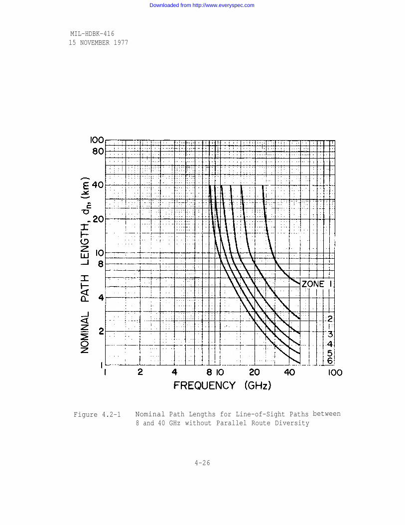
MIL-HDBK-41615 NOVEMBER 1977
Figure 4.2-1 Nominal8 and 40
Path Lengths for Line-of-Sight PathsGHz without Parallel Route Diversity
between
4-26
Downloaded from http://www.everyspec.com

15 NOVEMBER 1977
4.2.9 Consider Passive Repeaters
4.2.9.1 Passive repeaters are usually reflectors on hills adjacent to
a terminal. They are illuminated by an antenna on a short structure at
the terminal, and serve to provide the required terrain clearance where
this is not possible directly between terminals. They are also useful in
rough terrain where shorter paths are required to obtain the necessary
line-of-sight clearance, and can often replace an active repeater site.
4.2.9.2 Passive repeaters offer many economic and technical advan-
tages. Access problems are less important for a passive repeater
site than for an active repeater site since no primary power source and
little, if any, maintenance is required. Capital investment is also less
than for an active repeater but these savings may be partially countered
by increased power or antenna gain requirements at the active terminals
of the link. Primary advantages of passive repeater links are that
equipment requiring maintenance and logistic support can often be
placed in valleys for easy access and flexibility of location, and the
angle of penetration through the atmosphere to the passive repeater on
a nearby hill or mountain may be large enough to minimize multipath
fading (section 4.2.11).
4.2.9.3 Transmission loss for passive repeater paths will be lowest
when one leg of the path is much shorter than the other. The loss in
decibels, Lp, between antenna terminals at the opposite ends of a link
using a passive repeater may be approximately calculated as the sum
of the basic free-space transmission loss values for the two legs less
the sum of all antenna gains. The free-space loss, Lbf, is given by
[8] page 2-7:
L b f = 32.45 + 20 log f + 20 log d dB (4.2-1)
where d is in km and f is in MHz. (see also section 4.2.21).
4-27
MIL-HDBK-416
Downloaded from http://www.everyspec.com

MIL-HDBK-41615 NOVEMBER 1977
Then,
L p = 32.45 + 20 log f + 20 log d1 + 32.45 + 20 log f
+ 20 log d2 - G1 - G2 - 2Gp dB (4.2-2)
where G1is the gain of the antenna at site 1, G2 the gain at site 2, and
Gp is the gain of the aperture of the passive repeater projected perpen-
dicular to the propagation path. All gains are in dB relative to an
isotropic radiator, and the distances d1 and d2 in km are defined in
figure 4.2-2.
Figure 4.2-2 Typical Passive Repeater Configuration
The formula for Lp may be rewritten as follows:
L p = 64.9 + 40 log f + 20 log d1d2 - G1 - G2 - 2Gp. (4.2-3)
4.2.10 Consider the Number of Sites
4.2.10.1 Routes where the number of required sites is substantially
greater than that for other plausible routes may be eliminated since the
additional sites decrease system reliability and generally result in
increased costs.
4.2.11 Atmospheric Layer Penetration
4.2.11.1 A layer in the troposphere in which the atmospheric refraction
differs considerably from the refraction in adjacent layers may cause
sufficient bending of a radio beam to produce multipath or phase inter-
4-28
Downloaded from http://www.everyspec.com

MIL-HDBK-41615 NOVEMBER 1977
ference fading. This bending may be comparable to reflection when the
angle of incidence of the beam at such a layer is less than about 0.5°,
but at angles above 3° the effect is negligible. This angle of incidence
is sometimes referred to as the penetration angle. Unfortunately,
conditions conducive to atmospheric stratification often exist over flat
terrain where large penetration angles cannot be obtained without
excessively towers [3, page 61; 45, page 146]. Refractive structure of the
lower atmosphere is discussed in detail in Section 4.4.6.
4.2.11.2 If the take-off-angle of the antenna beam at the lowest site
above mean sea level (msl) is positive, it is the smallest angle of
penetration along the path. If the take-off-angle at the lowest site is
negative, the angle of penetration will be zero at some location along
the path.
4.2.11.3 The take-off-angle, is the angle between a horizontal line
extending from the center of an antenna and a line extending from the
same point to the other terminal antenna.
(4.2-4)
where all distances and heights must be in the same units.
h1 is the height of the lowest antenna above ms1.
h2 is the height of the other antenna.
d is the path length.
a is the effective earth radius.
4.2.12 Select Preliminary Routes
4.2.12.1 After careful study of topographic maps and considering the
other factors mentioned, the design engineer should choose a number
4-29
Downloaded from http://www.everyspec.com

MIL-HDBK-41615 NOVEMBER 1977
of possible routes that warrant further investigation. A typical diffi-
culty is that links selected for minimum fading potential or tower
heights will involve locating the sites in a remote area. Low levels of
man-made noise will also be obtained by locating sites in a remote
area; but this may result in poor site accessibility. Absolute guides
for selection cannot be given and the design engineer will have to weigh
the various considerations applicable to each path and make his prelim-
inary route selection on that basis.
4.2.13 Drawing Initial Terrain Profiles
4.2.13.1 Terrain profiles are prepared to verify that the selected
routes and sites are reasonable possibilities for LOS paths.
4.2.14 Map Scale
4.4.14.1 Even though the number of site and route possibilities being
considered at
most detailed
path profiles.
diverse; thus,
this point in the route selection involves many paths, the
maps available should be used for drawing the initial
The quality and scale of maps for various areas will be
uncertainty about some paths with marginal clearance
may only be resolved by the field survey.
4.2.14.2 Most large-scale and medium-scale maps have, in addition
to longitude and latitude coordinates, a grid system for locating or
referencing points. This grid system is
Transverse Mercator (UTM) grid and is
between 80 degrees south latitude and 84
detailed explanation of the UTM grid and
identified as the Universal
designed for world use
degrees north latitude. A
its application to military use
is given in [11] (pages
presented here.
4.2.14.3 The military
and numbers which indi
17 to 25); however, a brief general review is
grid reference consists of a group of letters
cate (1) grid zone designation, (2) the 100,000
meter (100 km) square identification, and (3) the grid coordinates of the
point expressed to the needed accuracy.
4-30
Downloaded from http://www.everyspec.com

MIL-HDBK-41615 NOVEMBER 1977
4.2.14.4 The UTM grid divides the world into large, geographic
areas (6 degrees E-W by 8 degrees N-S except that the region 72
degrees to 84 degrees N constitutes one area) which are designated as
the grid zones. The columns are numbered 1 to 60 consecutively and
the rows identified by letters alphabetically C through X (I and O
omitted). The grid zone designation of any area is determined by first
reading the column designation and then the row designation (see
figure 4.2-3).
4.2.14.5 Each grid zone is then divided into 100,000 m squares.
Each column of squares is identified by a letter, as is each row of
squares. Starting at the 180 degree meridian and proceeding easterly
along the equator for 18 degrees, the 100,000 m columns, including
partial columns along grid junctions, are lettered A through Z (omitting
the letters I and O), and are repeated at 18 degree intervals. The
100,000 m rows are lettered A through V (1 and O omitted) from south
to north. This partial alphabet for rows is repeated every 2,000,000 m.
Thus the identification of any 100,000 m square consists of two letters,
the first determined by reading horizontally and the second vertically.
4.2.14.6 The grid coordinates of a point within the grid square can be
expressed as precisely as desired, and are written as one number
always containing an even number of digits. The first half of the total
number of digits are read horizontally and the second half of the digits
vertically. The measurement used with a grid system is linear and the
unit of measure is usually the meter.
4.2.14.7 Example of a point identification within a UTM grid using a
military reference:
10S locates the grid zone designation
10SGF locates the 100,000 m square
10 SGF65 locates within 10,000 m square
4-31
Downloaded from http://www.everyspec.com

Figure 4.2-3
MIL-HDBK-41615 NOVEMBER 1977
4-32
Downloaded from http://www.everyspec.com

10SGF6558 locates within 1,000 m square
10SGF654576 locates within 100 m square
10SGF65415758 locates within 10 m square
4.2.15 Initial Path Profile Drawings
4.2.15.1 Correct site selection is based primarily on accurate path
profile determinations. These profiles normally show the longitudinal
center of the radio beam and a cross-section of the terrain along a
microwave path. For paths longer than 20 km, profiles should be
plotted along the great circle path between sites. Hills and ridges
near the great circle path must be taken into consideration, as well as
the terrain on the beam centerline. Critical points along the profile
should be plotted using the highest point on the horizontal arc defined
by ±0.5 degrees from the great circle path where the nearest site is
used as the vertex of the angle. Formulas for determining the great
circle path across maps are provided in section 4.2.16. A radio ray
in the vertical plane travels in a curved line which generally has a
radius of curvature greater than the true earth’s radius because of
atmospheric refraction. Refractive effects can generally be expressed
as changes in the effective earth’s radius (see section 4.4.6 for addi-
tional information on effective earth’s radius). Also, the effective
earth’s radius concept [17] and its derivation is treated in detail in
Volume I of [8]. For the purpose of determining required terrain
clearance and antenna heights, the ratio k of the effective to the actual
(physical) earth radius (aO = 6370 km) is used. Useful values of k for
initial design assumptions are infinity (corresponding to ducting
conditions), 4/3 (corresponding to a “standard atmosphere”), 1 and 2/3
(corresponding to “sub-refractive” conditions which are very unfavor-
able for line-of-sight links).
4-33
MIL-HDBK-41615 NOVEMBER 1977
Downloaded from http://www.everyspec.com

15 NOVEMBER 1977
4.2.15.2 The relationships between the microwave radio path and the
elevation profile are commonly presented by either of two methods.
One method is to prepare curvilinear graph sheets whose curvature
corresponds to the applicable k-factor. On this paper, the radio beam
axis is presented as a straight line. This method has often been used
in the past, but has disadvantages because of limitations in the choice
of scale and in the somewhat restricted choice of k-factors on generally
available graph sheets. Alternatively, special graph sheets must be
prepared for each required value of k. The second method, particular-
ly recommended for LOS paths, is to plot the terrain elevations as a
function of path distance on linear graph paper. Here, any convenient
vertical and horizontal scales can be used, and the profile may usually
be plotted on 8-1/2 x 11 inch paper. For such a plot, a straight line
beam axis represents an effective earth radius equal to “infinity”.
Beam axes representative of other k values can then be plotted as
curved lines with the points as displacements below the line represent-
ing k = These values of displacement, h, are calculated using either
of the following equations:
or
(4.2-5)
(4.2-6)
where h is in meters, d1 and d2 are distances from a point along the
path to each terminal and are in kilometers, the effective earth’s
radius, a, is in kilometers, and k is the non-dimensional effective
earth’s radius factor. Figure 4.2-4 is a typical example of a profile
plotted using this method.
4.2.15.3 All maximum elevation points on the profile should be care-
fully checked and symbols for trees or other vegetation used if the maps
4-34
MIL-HDBK-416
Downloaded from http://www.everyspec.com

Figure 4.2-4
MIL-HDBK-41615 NOVEMBER 1977
4-35
Downloaded from http://www.everyspec.com

MIL-HDBK-41615 NOVEMBER 1977
indicate their presence. Vegetation, unless very sparse, at micro-
wave frequencies is almost impenetrable to radio frequency energy,
and should be added to the profile elevations so that the top of the
vegetation can be used in evaluating terrain clearance. Similarly, if
large buildings or clusters of man-made objects are present in the
path they should be drawn on the path profile at their actual height.
4.2.15.4 A line-of-sight path that clearly has no obstructions to the
radio beam is an excellent candidate for the system; however, paths
having obstructions that make the path marginal (especially those for
k < 2/3) should not be dismissed, but marked for further investigation
until other aspects of the system are investigated. Marginal paths may
often be made line-of-sight by increase in
ends of the path.
4.2.16 Plotting a Great Circle Path
4.2.16.1 The spherical triangle used for
tower height at one or both
the computation of points on
a great circle path is identified on figure 4.2-5 as PAB. A and B are
the antenna terminals, and P the north or south pole. B is selected to
have a greater latitude than A, and P is in the same hemisphere. The
triangle shown is for the northern hemisphere but may readily be
inverted to apply to the southern hemisphere. B' is any point along the
great circle path from A to B, and the triangle PAB' is the one actually
solved. The latitudes of the points are denoted by
while C and C' are the differences in longitude between A and B and
A and B', respectively. Z and Z' are the corresponding great circle
path lengths. The following formulas are practical for hand computa-
tions as well as for digital computers. Equations 4.2-7 to 4.2-10 have
been taken from [1] (pp. 26-9 to 26-11).
4.2.16.2 The initial bearings or azimuth values (Xfrom terminal A, and Y from
terminal B) are measured from true north, and are calculated as follows:
4-36
Downloaded from http://www.everyspec.com
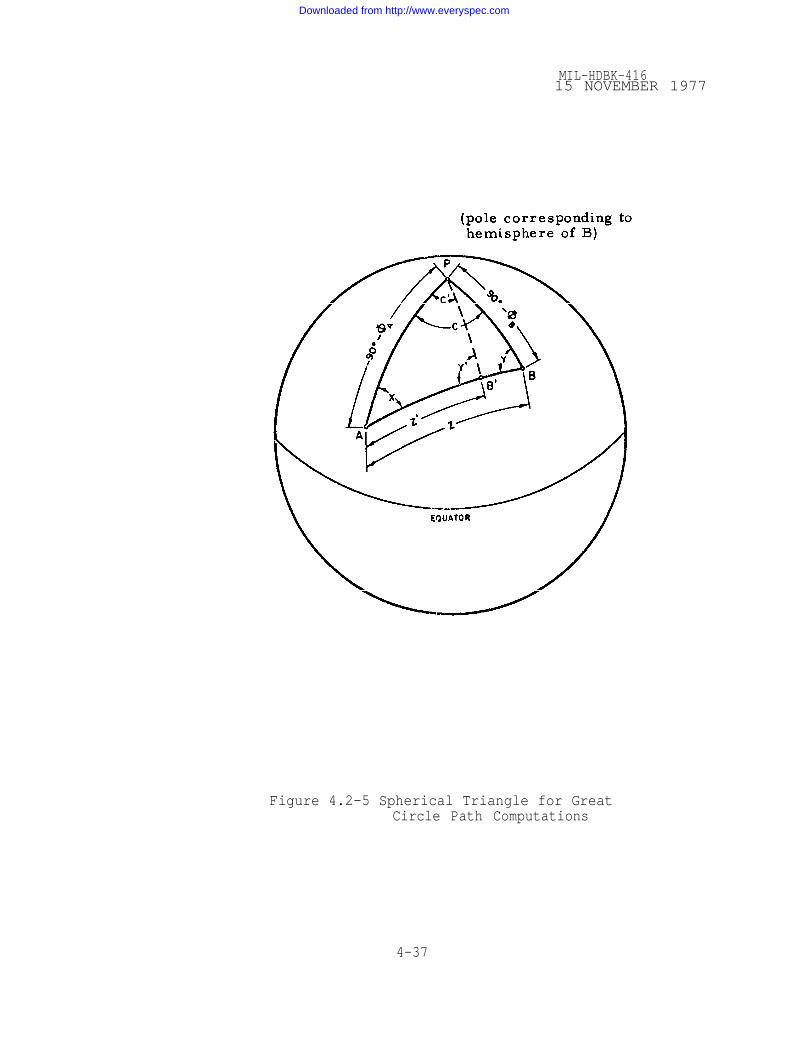
MIL-HDBK-41615 NOVEMBER 1977
Figure 4.2-5 Spherical Triangle for GreatCircle Path Computations
4-37
Downloaded from http://www.everyspec.com

MIL-HDBK-41615 NOVEMBER 1977
(4.2-7)
(4.2-8)
(4.2-9)
The great circle distance, Z (in degrees), is given by
4.2.16.3 To convert the angle Z obtained in degrees from (4.2-10) to
kilometers of length, the following is used:
d k m= 111.12 Z°. (4.2-11)
4.2.16.4 The following formulas show how to calculate either the
latitude or the longitude of a point on the great circle path, when the
other coordinate is given. The given coordinates correspond to the
edges of detailed maps, and to intermediate points usually about 7.5
minutes apart, so that straight lines between points will adequately
approximate a great circle path.
4.2.16.5 For predominantly east-west paths, calculate the latitude
for a given longitude difference C':
cos Y' = sin X sin C' sin - cos X cos C' (4.2-12)
cos = sin X cos sin Y'. (4.2-13)
4.2.16.6 For predominantly north-south paths, calculate the longi-
tude difference C' for a given latitude :
4-38
Downloaded from http://www.everyspec.com
MIL-HDBK-41615 NOVEMBER 1977
(4.2-14)
(4.2-15)
Where the bearing of a path is close to 45 degrees, either method may
be used.
4.2.17 Path Clearance
4.2.17.1 When the atmosphere is sufficiently sub-refractive (large
positive values of the refractive index gradient), the ray paths will be
bent in such a way that the bulge of the earth, or specific terrain
features, appear to block the path between transmitter and receiver.
In such cases, there is no longer a line- of-sight ray path, and energy
transfer between the terminals is by diffraction over the terrain. The
loss in signal under such conditions has been called diffraction fading.
It may be alleviated by installing antennas which are so high that even
the most severe ray bending will not interpose obstacles to the direct
ray path.
4.2.17.2 Diffraction theory applicable to near line-of-sight analysis
indicates that the direct path between the transmitter and the receiver
needs a clearance above ground of at least 60 percent of the radius of
the first Fresnel zone to approximate near free-space propagation
conditions. Making allowance for possible sub-refraction is usually
done by ensuring that the required clearance is maintained even when
the effective earth radius is reduced below its normal value. Radio
link designers in the United States and the United Kingdom often require
that 60 percent of the first Fresnel zone radius shall be clear of inter-
vening terrain even when the effective radius of the earth is reduced
to 4500 kilometers (k = 0.7) [7] (pp. 115 and 116). When statistics of
occurrence of sub-refractive conditions are known, it is possible to
4-39
Downloaded from http://www.everyspec.com

MIL-HDBK-41615 NOVEMBER 1977
replace this “rule-of-thumb” by more accurate procedures which take
into account the actual time distribution of sub-refractive gradients in
specific areas.
4.2.17.3 Path clearance near the antennas should be considered in
terms of three-dimensional beam clearance. A good model for the
beam volume near a terminal is a cylinder having a cross-section of
the same shape and dimensions as the antenna aperture. The antenna
and beam volume should generally be kept at a minimum of three meters
above the ground at the site. This precaution should be taken to pre-
vent radiation hazards as well as to prevent beam blockage by people,
vehicles, security fences, etc.
4.2.18 Fresnel Zones
4,2.18.1 The Huygens-Fresnel wave theory states that the electro-
magnetic field at a point, S2, (figure 4.2-6) is due to the summation of
the fields caused by reradiation from small incremental areas over a
closed surface about a point source, S1, provided S1 is the only
primary source of radiation. The field at a constant distance, r1, from
S1 (a spherical surface) has the same phase over the entire surface
since the electromagnetic wave travels at a constant speed in all
directions in free space. This constant phase surface is called a
wave front. If the distances, r2, from various points on the wave front
to S2 are considered, the contributions to the field at S2 will be seen
to be made up of components that add vectorially in accordance with
their relative phase differences. Where the various values of r2
differ by (half wavelength), the strongest cancellation occurs.
Fresnel zones distinguish between the areas on a closed surface about
S1 which add and those which cancel.
4.2.18.2 Consider a moving point, P, in the region about the terminal
antenna locations S1 and S2 such that the sum of the distances r1 and r2
4-40
Downloaded from http://www.everyspec.com

Figure 4.2-6
MIL-HDBK-41615 NOVEMBER 1977
4-41
Downloaded from http://www.everyspec.com

MIL-HDBK-41615 NOVEMBER 1977
from the antennas to P is constant. Such a point will generate an
ellipsoid with S1and S2 as its foci. Now define a set of concentric
ellipsoidal shells so that the sum of the distances r1and r2 differs by
multiples of the half wavelength The intersection of these ellisoids
with any surface defines Fresnel zones on the surface. Thus, on the
surface of the wave front, a “first” Fresnel zone F1 may be defined as
bounded by the intersection with the sum of the straight line segments
r1 and r2 equal to the distance d plus one-half wavelength
second Fresnel zone, F2, is defined by the region where r1 + r2 is
greater than d + and less than d + Thus, Fn is the region
where r1 + r2 is greater than d + (n - 1) but less than d + n
Field components from even Fresnel zones tend to cancel those from
odd zones since the second, third, and fourth zones, etc., are approxi-
mately equal in area.
4.2.18.3 The concept of Fresnel zones is not meaningful for the “near
field” within short distances of practical antennas. A rule of thumb
for determining the minimum distance, dF, at which the zones become
meaningful is that dFbe greater than where D is the maximum
dimension of the antenna aperture in the same units of length as
4.2.18.4 A good approximate equation (valid for almost all microwave
applications) for the outside boundary of the nth Fresnel zone radius, Rn,
on a surface perpendicular to the propagation path is
or
(4.2-16)
(4.2-17)
In the first equation all distances and the wavelength must be in the
same units. must be small compared to the distance and antenna heights
involved, and r1+r2 (from paragraph 4.2.18.2) should not be significantly
larger than d1 +d2. In the second equation all distances are in kilometers,
4-42
The
Downloaded from http://www.everyspec.com

MIL-HDBK-41615 NOVEMBER 1977
the frequency is in GHz and the Fresnel zone radius
Rl is the radius of the first Fresnel zone, then
is in meters. If
(4.2-18)
Because the higher numbered zones tend to be self canceling, they are
not significant for many calculations; however, consideration of the
higher order zones is helpful in understanding obstacle diffraction, or
the use of diffraction gratings as passive repeaters (see sect. 4.4. 39).
4.2.19 Terrain Reflections
4. 2.19.1 Potential reflection surfaces can often be identified by
examination of terrain profiles; also the blockage of reflected signals
by terrain obstacles may be evaluated in this manner. However, the
magnitude and other characteristics of terrain reflections may either
be specular (from a smooth surface) or scattered (from a rough sur-
face). A smooth surface is one for which the phase difference between
reflected component rays is small, resulting in an almost unperturbed
plane-wave being reflected. A rough surface imparts considerable
phase shift to the individual rays, resulting in partial interference
between them which will produce an irregular scattering pattern.
4.2.19.2 The Rayleigh criterion is often used to determine whether a
surface will produce a mainly scattered or a specular reflection. The
reflection is considered specular if
where is the standard deviation of the
surface, is the wavelength and a is the
must be in the same units.
' (4.2-19)
differences in height of the
angle of incidence.
4. 2.19.3 Terrain roughness parameters applicable to practical micro-
wave links may vary greatly with time and season; i. e. , ground
4-43
Downloaded from http://www.everyspec.com

MIL-HDBK-41615 NOVEMBER 1977
reflection coefficients and roughness will vary with snow cover, air
humidity and temperature immediately above the ground, and with the
period in the life cycle of ground cover vegetation. Effective “roughness”
of water surfaces will vary with wave height.
4.2.19.4 A word of caution when considering Fresnel zones in connec-
tion with surface reflections: the Fresnel ellipsoids to be considered
are those concentric about the line between one antenna and the image
relative to the reflecting surface of the other antenna.
4.2.19.5 Reflections from terrain should be avoided if at all possible.
Useful techniques are selection of paths with maximum terrain clear-
ance and use of narrow beam antennas, although extremely narrow
beams may cause fading by atmospheric defocusing. If terrain reflec-
tions cannot be avoided, the adverse effects can be greatly reduced
through the use of vertical space or frequency diversity. More detailed
analysis and information regarding reflections from terrain may be
found in [41].
4.2.20 Initial Path Loss Estimates
4.2.20.1 Following ATT practices, “path loss” as used here is defined
as the ratio of the power supplied to the terminals of the transmitting
antenna to that available at the terminals of the receiving antenna.
Path loss estimates must include consideration of the antenna beam
characteristics, not only in terms of the power gains, but also in
terms of the relations between the beam dimensions and the path geom-
etry. The antenna beam width ( the width at the half-power points)
defines the cross section of the radio path and therefore the amount of
terrain or atmosphere relevant to calculating or estimating path loss.
4.2.20.2 Many types of propagation effects produce attenuation or
distortion of a radio signal; they include the physical phenomena of
divergence, absorption, diffraction, reflection, and refraction. The
4-44
Downloaded from http://www.everyspec.com

MIL-HDBK-41615 NOVEMBER 1977
attenuation or weakening’ of microwave signals over line-of-sight paths
can be classified in terms of constant and time-varying losses (fading).
Understanding of these losses will contribute toward making reasonably
accurate path loss estimates.
4.2.20.3 Some components of path loss are relatively constant.
Examples are those due to the divergence of radiation from an antenna
(which varies directly with the square of the distance), certain types of
atmospheric absorption, some types of terrain reflections, and beam
blockage near the antennas.
4.2.20.4 Time-varying losses include power fading and multipath
fading (phase interference due to differences in component path delays).
Within the classification of power fading are rain attenuation, water
vapor absorption, beam deflection away from the desired antenna
because of atmospheric reflection or refraction, and the terrain block-
age associated with beam deflection caused by atmospheric refractivity
changes. Multipath fading consists of phase interference between
signals arriving over more than one path which are diffracted, reflected
or refracted by changing atmospheric effects over each path. An
important type of multipath fading is the fading from rain because of
appreciable doppler shift in the reflected signals which causes distor-
tion as well as attenuation of a broadband signal. The extent to which
a modulated signal can be degraded because of scattering from rain is
unknown at this time.
4.2.21 Free Space Basic Transmission Loss and Free Space Path
Loss
4.2.21.1 The loss due to the divergence of radiation from a point in
free space may be calculated by using the mathematical model of
isotropic antennas (antennas which radiate energy equally in all direc-
tions) separated by the path length and isolated in free space. The
4-45
Downloaded from http://www.everyspec.com

MIL-HDBK-41615 NOVEMBER 1977
loss between terminals of such hypothetical antennas is called the free
space basic transmission loss, Lbf’
and is expressed in decibels.
Lbf = 92.45 + 20 log fGHz + 20 log dkm dB (4.2-20)
This is the same expression (4. 2-1) already given in section 4.2.9,
except that here the frequency f is in gigahertz. As before, d is the
path distance in kilometers. The solution to this equation is presented
graphically in figure 4. 2-7 for various frequencies and distance ranges.
4.2.21.2 The free space path loss Lof is defined here as the loss
between the two antenna terminals in free space provided that the
antennas are loss-free and properly impedance-matched to the trans -
mitter and
in the case
space path
receiver, respectively. These conditions are normally met
of well-designed microwave line-of-sight links. The free-
loss Lof is obtained by subtracting the maximum power
gains, Gt and Gr in dB, of the transmitting and receiving antennas
from Lbf, the free space path loss.
L = L - G - G d B (4.2-21)of bf t r
The power gain of an antenna in a specified direction is times the
ratio of the power radiated per unit solid angle in that direction to the
net power accepted by the antenna from its generator. A more com-
plete discussion of antenna gain is given in [ 18] (p. 19), and will be
presented in section 4.4.29.
4.2.22 Atmospheric Absorption
4.2.22.1 The path loss component caused by atmospheric absorption
primarily due to oxygen and water vapor, varies with air density,
temperature and humidity. Since oxygen absorption loss is dependent
only upon air density and path length, this loss is fairly stable as a
function of time. Water vapor absorption is more variable with time.
4-46
Downloaded from http://www.everyspec.com
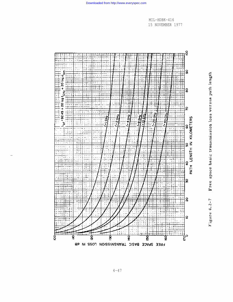
MIL-HDBK-41615 NOVEMBER 1977
-
4-47
Downloaded from http://www.everyspec.com
MIL-HDBK-41615 NOVEMBER 1977
The values of absorption for oxygen, yoo, and water vapor, ywo, are
shown in figure 4.2-8 in decibels per kilometer as a function of fre-
quency.
4.2.22.2 For frequencies between 1 and 10 GHz, as estimate of
0.01 dB per kilometer path length is a reasonable allowance for the
total atmospheric absorption. Between 10 and 40 GHz the values of
figure 4.2-8 are added together and then multiplied by the path length
to estimate the value of the average atmospheric absorption. For paths
located at high terrain elevations, or for paths with elevation angles
greater than 0.5 degrees, such an estimate will be slightly too large.
For a first estimate, the values from figure 4. 2-8 will generally be
sufficient even though the losses will vary with humidity and air
density.
4.2.22.3 The upper limit of attenuation due to fluctuations in the water
vapor content of the air is approximately one and one-half times that
shown by the curve for y Wo. because the upper limit is based on higher
temperatures and greater relative humidity. It should be remembered
that conditions for maximum water vapor absorption will often coincide
with those producing additional attenuation because of rain.
4.2.23 Attenuation Due to Precipitation
4.2.23.1 The attenuation of radio waves by suspended water droplets
and rain often exceeds the effects of combined oxygen and water vapor
absorption. Water droplets in fog or rain will scatter radio waves in
all directions whether the drops are small compared to the wavelength
or comparable to the wavelength. In the latter case, raindrops trap
and absorb some of the radio wave energy; accordingly, rain attenua-
tion is much more serious at millimeter wavelengths (frequencies
above about 10 GHz) than at lower frequencies.
4-48
Downloaded from http://www.everyspec.com

MIL-HDBK-41615 NOVEMBER 1977
PRESSURE 760mm HgTEMPERATURE 20°C
WATER VAPOR DENSITY 10g/m3
FREQUENCY IN GHz
Figure 4.2-8 Surface values 700 and ~wo of
absorption by oxygen and watervapor
4-49
Downloaded from http://www.everyspec.com

MIL-HDBK-41615 NOVEMBER 1977
4.2.23.2 The attenuation effects of rain, while small in the lower
microwave region, become more important at frequencies above 10
GHz. In Japan, for example, at 15.4 GHz, a uniform rain falling at
the rate of 100 mm/hr has been observed to produce an excess attenua-
tion of about 7 dB/km [87]. In the United States, over a 407 km path
at 14.4 GHz, as much as 48 dB attenuation was observed at a time
when the average rainfall rate was 137 mm/hr [19]. Also in the United
States, a uniform rain, falling at the rate of 100 mm/hr was observed
to produce an excess attenuation of about 9 dB/km at 18 GHz [16].
Under these conditions, it is obviously impossible to maintain transmis-
sion over paths longer than a few kilometers. However, recent investi-
gations have shown that the temporal and spatial distributions of such
severe rain storms are highly restricted [16], and therefore parallel
paths a few km apart may provide an effective diversity improvement
(see paragraph 4.2.6.2). The excess attenuation caused by rainfall is the
controlling factor above 15 GHz; therefore, radio relay systems operat-
ing at these frequencies will have to employ short hops if they are to
have a high degree of reliability (see figure 4.2-1).
4.2.23.3 Conventional diversity configurations, either vertical space
or frequency diversity, cannot be used to minimize the effects of rain
attenuation. Route diversity configuration may be used. Such methods
of obtaining reliability above 10 GHz are expensive but are worthy of
consideration.
4.2.24 Estimating Rain Attenuation
4.2.24.1 To estimate time distributions of rain attenuation fading for
a path in a given area, it is necessary to know three things: one, the
attenuation per kilometer as a function of rainfall rate (figure 4.2-9);
two, the time distribution of rainfall rates for the geographic area
(figure 4.2-10 together with 4.2-11); and three, the spatial distribution
4-50
Downloaded from http://www.everyspec.com
MIL-HDBK-41615 NOVEMBER 1977
of rain rates. The information for figure 4.2-9 showing attenuation
per kilometer was obtained from [7] p. 179. The time distributions of
rainfall rates and the zone map of the continental United States (figures
4.2-10 and 4.2-11) were computed from statistics on maximum five
minute rainfall rates expected once in two years [19].
4.2.24.2 In order to make the use of the information from these
figures more convenient, time distributions in terms of attenuation per
kilometer (see figures 4.2-12a to c) have been prepared for each zone
(figure 4.2-11) from the rain rate- time distributions (figure 4.2-10)
and the graph of rain attenuation as a function of rain rates (figure
4.2-9). A rough estimate of the time distribution of rain attenuation
for a given path may be obtained by multiplying the length of the path,
or 10 kilometers, whichever is less, by the ordinate values of attenua-
tion per unit of length. The 10 kilometer limit is based on estimates
of average storm cell diameters. These distributions will provide
one of the components in the estimation of fading depth when making
initial path loss calculations.
4.2.24.3 Figure 4.2-13 is a map of the world showing rain zones
defined in a similar manner as those used for the United States
(figure 4.2-11). It is not intended to provide the detail required for
design of systems in a particular locality; rather, it should be used as
a rough indicator of the general areas in which rain attenuation may be
a significant design consideration. For most parts of the world,
precipitation rate data are either very limited or not available; this
rain zone map is based primarily on maximum one-hour rain data of
reference [21] but also includes information based on work presented
in [22 - 27]. Terrain effects are important considerations in the
interpretation of this map, particularly in the case of relatively small
but mountainous islands. Note, for example, that Hawaii is identified
4-51
Downloaded from http://www.everyspec.com

Figure 4.2-9 Rain attenuation versus rainfall
rate between 5 and 100 ghz
4-52
MIL-HDBK-41615 NOVEMBER 1977
Downloaded from http://www.everyspec.com

MIL-HDBK-416
15 NOVEMBER 1977
Figure 4.2-10 Rainfall rate-time distributions
for six climatic zones
4-53
Downloaded from http://www.everyspec.com

MIL-HDBK-41615 NOVEMBER 1977
4-54Figure 4.2-11
Downloaded from http://www.everyspec.com

MIL-HDBK-41615 NOVEMBER 1977
4-55Figure 4.2-12a
Downloaded from http://www.everyspec.com
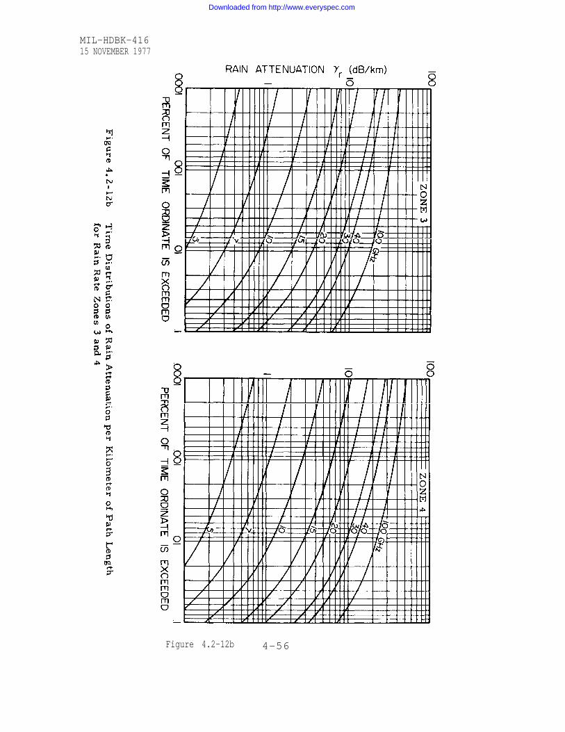
MIL-HDBK-41615 NOVEMBER 1977
4-56Figure 4.2-12b
Downloaded from http://www.everyspec.com

MIL-HDBK-41615 NOVEMBER 1977
4-57Figure 4.2-12c
Downloaded from http://www.everyspec.com

MIL-HDBK-41615 NOVEMBER 1977
4-58
Figure 4.2-13
Downloaded from http://www.everyspec.com
MIL-HDBK-41615 NOVEMBER 1977
by zones 3 - 6. Slopes exposed to the prevailing (trade) winds may
have very heavy average rainfall while areas on the lee side of the
islands may be quite dry. Similar climatic modifications also occur
on the larger land masses, i. e. , when moist winds are lifted by a
mountain chain, the windward slopes tend to have heavier precipitation
than the lee side. Also, in mountainous regions precipitation tends to
increase with altitude [31]. An increase in precipitation probability
in Colorado averaging nearly five percent per 1000 feet elevation gain
(during July and August) was reported in [32].
4.2.24.4 Rainfall attenuation estimates for regions outside the United
States should, whenever possible, be based upon rainfall rate or
attenuation data available from ETAC (USAF Environmental Technical
Application Center) or foreign meteorological services and radio
propagation laboratories. The rainfall zone information shown in
figure 4.2-13 in conjunction with the attenuation curves for the United
States (figure 4. 2-11) will provide only rough estimates.
4.2.25 Atmospheric Refraction
4.2.25.1 Changes in atmospheric refraction sometimes cause severe
fading on line-of-sight microwave radio links. For detailed information
on this topic, see section 4.4.6. The gross behavior of the variation
in transmission loss for many paths is explained by means of two
relatively basic propagation mechanisms: refraction associated with
the time-varying vertical gradient of refractive index and the forma-
tion of phase-interference patterns because of diffraction and reflection
by the earth's surface and atmospheric refractive index discontinuities.
Refraction can also cause fading when extreme conditions cause the
ray to arrive at an angle off the main-beam axis of the receiving
antenna (par. 4.2.25.3).
4-59
Downloaded from http://www.everyspec.com

MIL-HDBK-41615 NOVEMBER 1977
4.2.25.2 Measurements of the vertical refractive-index gradient in
the lower layers of the atmosphere show that the range of values is
extremely large. The following statement is taken from [7], page 115:
“In the United States, at Cape Kennedy, Florida, the vertical gradient
was measured in the first 100 meters near the surface of the earth.
It was found to vary between +230 N units/km, which was exceeded
0.05 percent of the time, and -370 N units/km, which was exceeded
during 99.9 percent of the time, which corresponds to k values of
0.4 and -0.7 respectively. ” These variations are typical for most
parts of the world but the very extreme values need not always be
allowed for in system design because of their limited extent in time
and space. For most parts of the world gradient variations between
+70 and -140 N units/km (corresponding to O. 7 10) are more
typical.
4.2.25.3 Variation of atmospheric refraction can cause changes in
the apparent angle-of-arrival of the line-of-sight ray particularly in
the vertical plane, and can therefore cause effectively a reduction in
gain in the antennas used at the radio path terminals. Measurements
made in the United States over a path of 28 kilometers, at frequencies
of 4 and 24 GHz, show that the angle-of-arrival can change rapidly by
as much as 0.75 degrees above and below the normal line of sight
[7], page 117. The angle-of-arrival variation in the horizontal
plane is usually much less, being of the order of 0.1 degrees.
Measurements in other parts of the world show less variation, but
generally the variations become larger as the climate becomes hotter
and more humid. Because of the vertical variations in angle-of-
arrival, antennas having half-power beamwidths less than 0.5 degrees
should generally be avoided for line-of-sight paths. This limitation
can be used as one criterion to determine maximum aperture size for
4-60
Downloaded from http://www.everyspec.com

MIL-HDBK-41615 NOVEMBER 1977
antennas and the maximum vertical dimension for passive repeaters
(fig. 4.4-33). Note that the dimensions for antennas are given in feet
because of the nominal values generally available from U.S.
manufacturers.
4.2.26 Multipath Fading
4.2.26.1 Multipath effects occur in two forms: reflection from the
ground or water surfaces, and refraction or reflection by inhomogenei-
ties in the atmosphere.
4.2.26.2 Under some circumstances, the direct ray will be interfered
with by the ground-reflected ray or other multipath rays. The most
severe fading occurs when there are two effective components of the
same order of magnitude varying in their relative phase. Measure-
ments made in the United States show that as many as six significant
components may exist at one time [84].
4.2.26.3 Multipath propagation measurements carried out in Japan
[85] show that most of the deep fades are caused by destructive inter-
ference between two dominant rays and that the path-length difference
between these rays varies to a considerable extent from path to path.
Maximum path length differences on the order of many wavelengths
can be observed on oversea as well as on overland paths.
4.2.26.4 Very severe fading can occur on over-water paths when the
point of specular reflection falls on the water. If such a path cannot be
avoided, height or frequency diversity may be used to reduce the
severity of the fading. Alternatively, fading can be reduced consider-
ably if the geometrical point of reflection on the water is screened
from one or the other of the terminals by the terrain (even if some of
the surface of the water is still visible from both terminals). However,
experience on one over- water path 80 kilometers long showed that it
was very difficult to achieve transmission of complex signals, such as
4-61
Downloaded from http://www.everyspec.com

MIL-HDBK-41615 NOVEMBER 1977
color television, if the water surface was not completely invisible from
at least one terminal [86].
4.2.26.5 Under normal conditions and over moderately rough sea or
irregular terrain, one expects a portion of the ground-reflected wave
to be scattered out of the propagation path. However, when the atmos-
phere is super-refractive and the surface appears concave, the
reflected wave is enchanced by the convergence of the associated rays.
4.2.26.6 In addition, experiments in Germany have revealed that
total reflection can occur in an atmospheric layer near the ground,
this layer being connected mostly with mist or ground fog experienced
over moist river valleys or moors [88]. Some earlier work carried
out in The United Kingdom also shows correlation between fading and
ground fog [89].
4.2.26.7 The frequency of occurrence and observation of multipath
fading caused by layering in the atmosphere is related to the variation
of the structure of refractive index with time; i. e. , the worst propaga-
tion conditions are likely to occur during periods of extreme stratifica-
tion of the atmosphere. On overland paths and in temperate climates,
such conditions normally exist during the night and early morning hours
of summer days. Reflections from rapid changes of the refractive
index within a height range of several tens of meters above the surface
of the earth can be a source of multipath propagation.
4.2.26.8 For designing radio relay systems conforming to DCA
Standards it is often necessary to predict the probability of outages due
to deep fades for very small percentages of the time (i. e. , on the
order of 0.01 percent for an average hop of about 50 kilometers). If
dual vertical space diversity or dual frequency diversity is used and
fades on the two sets of equipment are not well correlated, prediction
of the probability of the fade depth must be made for approximately
4-62
Downloaded from http://www.everyspec.com

MIL-HDBK-41615 NOVEMBER 1977
0.01 percent of the time. Although diversity aids in preventing outages
caused by interference fading, outage time cannot be directly equated
to depth and frequency of fading of the combined signal because multi-
path causes distortion as well as attenuation. The fading depth
exceeded for a small percent of the time increases with path length and
increases slightly with frequency. Multipath fading is also a function
of the terrain near the path, the atmospheric conditions, and the angle
of penetration through the atmosphere.
4.2.26.9 Fades due to non-linear refractive index gradients (stratified
atmospheric layers) are usually also of the multi path, phase inter-
ference type, and can occur even when there are no reflections from
terrain. A combination of ray paths caused by both ground and atmos-
pheric layer reflections can produce very severe fading. Non-linear
refractive index gradients are most likely to occur during the night,
with light winds, clear skies, and high humidity near the surface.
4.2.27 Estimating Multipath Fading
4.2.27.1 An empirical formula based on the work by Barnett [83] and quoted
in [4; see p. 119] can be used to estimate the percentage of time within a
year, Pmf, that fades exceed a specified depth below free space for a given
path and frequencyo This formula applies to paths within the United States,
and does not specifically consider beam penetration angle through the
atmosphere or the beam clearance of terrain:
Pmf= a x b xwhere -
1/2 :b = 1/4 :
1/8 :
6.0 X 10⁻⁵ X f x d3 x 10-mf/10% (4.2-22)
for very smooth terrain, including overwaterfor average terrain, with some roughnessfor mountainous, very rough or very dry terrain
gulf coast or similar hot, humid areasnormal interim temperate or northern climatemoutainous or very dry climate
4-63
4 :a= 1 :
1/4 :
Downloaded from http://www.everyspec.com

MIL-HDBK-41615 NOVEMBER 1977
f= frequency in GHzd= path length in kmMf= fading depth exceeded below free= space level, in dB.
Note that for performance calculations as outline in section 4.5 the
longterm median level Pr(0.5) should be used as a reference level
instead of the free-space level.
4.2.27.2 The above formula has been checked by measurements In the
4, 6, and ll GHz bands [83]. A similar type formula is provided in
[7], p. 119, based on measurements made in Japan.
4.2.28 Combining Path Loss Contributions and Grading Paths
4.2.28.1 For the initial comparative evaluation and ’’grading” of
potential links, only minimum tower heights should be used, which are
sufficient for clearing local obstacles such as tree or buildings. In
this manner, all potential paths can be compared on a common basis.
Paths with insufficient clearance should be rejected outright unless no
better paths are available.
4.2.28.2 For each path, those path loss contributions in decibels
should be added up which are relatively constant with time. These are
the free-space loss LOf(see section 4.2.21) and the average oxygen
absorption from section 4.2.22. Allowances for multipath and other
fading conditions may also vary between potential links of a system,
and these will be discussed in the following sections. In general,
conditions favorable for the formation of heavy rain showers tend to
mix the lower atmosphere and eliminate multipath fading, particularly
on short links which will normally be used at frequencies above 15 GHz.
However, on very long LOS links, the simultaneous occurrence of
fading due to multipath and rain is more likely. Resulting total path
loss values are then compared and those paths with the lowest values
4-64
Downloaded from http://www.everyspec.com

MIL-HDBK-41615 NOVEMBER 1977
are selected unless other considerations apply. For paths over 10 km
long, the largest estimate for water vapor absorption should be added
to the distribution for rain attenuation loss because these losses are
likely to occur at the same time.
4.2.29 Fading Estimates for Long LOS Links
4.2.29.1 It may be necessary at times to design long line-of-sight
links because of inaccessible or otherwise unusable terrain (for relays),
or systems extending over large bodies of water. In order to achieve
line-of-sight conditions over paths as long as 200 km, terminals must
be located on mountain tops. For such paths, atmospheric and terrain
characteristics at and near mid-path is usually very critical since the
clearance between the ray path and the terrain is at a minimum, and
also because the angle of penetration between the ray path and the
atmospheric layers is small. Particularly if the midpath region is over
water or broad river valleys, small penetration angles in conjunction
with atmospheric stratification can produce severe fading which is
sometimes quite prolonged (hours or days) because of defocusing of the
energy, or trapping of energy in surface or elevated ducts so that the
desired terminal cannot be reached.
4.2.29.2 Although the literature contains may qualitative statements
regarding fading on long LOS links, few specific recommendations for
design exist. In general, recommendations call for greatest possible
terrain clearance at any point of the path, particularly for over-water
links, since strongest s gratification exists usually near the surface. A
minimum clearance of 50 m between the ray path and the terrain is
recommended [4] p. 52. However, this is an arbitrary figure, and
would not necessarily apply to any type of terrain and to all atmos-
pheric conditions.
4-65
Downloaded from http://www.everyspec.com
MIL-HDBK-41615 NOVEMBER 1977
4.2.29.3 For frequencies between 2 and 7 GHz, some quantitative
information has been derived in [3] (p. 63) for long paths. Three cate-
gories of fading are described (A, B, and C), and curves of expected
fading depths versus path distance are shown in figure 4.2-14 for
0.1 percent and 1 percent of the time during the month with most
severe fading.
Curve A - type-A fading relates to hops with “favorable” fading
characteristics:
rare occurrence of atmospheric stratification;
rare occurrence of calm weather;
above hilly country, but not above wide river valleys and
inland lakes;
in high mountainous country, with radio paths high above the
valleys;
for hops between points in a plain or a valley and mountain
tops where the angle of elevation relative to the horizon-
tal plane exceeds approximately 0.5° for the lower
station;
Curve B - type-B fading relates to hops with “normal” fading charac-
teristic:
above flat country if stratification is formed only occasionally;
above hilly country, but not above wide river valleys and
inland lakes;
in coastal areas with moderate temperatures but not over
the sea;
for hops with a steep angle of elevation also in hot and tropi-
cal regions;
Curve C - type-C fading relates to hops with “unfavorable” fading
characteristics:
4-66
Downloaded from http://www.everyspec.com

MIL-HDBK-41615 NOVEMBER 1977
4-67Figure 4.2-14
Downloaded from http://www.everyspec.com

MIL-HDBK-41615 NOVEMBER 1977
above humid areas where ground mist is apt to form and
especially to hops with a flat path above flat ground; for
example, wide river valleys, moors;
near the coast in hot regions and, generally, in tropical
regions, to hops not operating with a large angle of
elevation over-water links.
4.2.29.4 The information in figure 4.2- 14 is provided to estimate fad-
ing depths that are exceeded for small percentages of time for paths up
to 150 km, and is based on information in [3]. Since much of this fading
is due to multipath, the outage time represented by the fading depths in
figure 4.2-14 can be reduced using either frequency or space diversity.
4.2.30 Additional Route Considerations
4.2.30.1 After grading potential links and making comparisons on the
basis of profiles and path loss distributions, certain sets of these links
will form routes which will appear good choices for further evaluation.
Additional factors that must be considered and weighed carefully for
their contribution in system performance are (1) localized meteorologi-
cal conditions and detailed path clearance conditions, both present and
future, (2) possible tower height and construction restrictions, (3)
potential radio interference, and (4) security requirements in the area.
4.2.31 Meteorological and Climatological Data
4.2.31.1 The climate of the area may suggest potential difficulty in
site accessibility. AS an example, the average and maximum snow
depth in the area should be determined from climatological records.
Note that there is a difference between snow depth and snowfall, the
latter referring to the accumulated total if no melting or settling
(packing) has occurred. There may be large differences in snow depths
observed at a valley station and on an adjacent high ridge. Local
farmers, ranchers, and forestry officials are good sources of
4-68
Downloaded from http://www.everyspec.com

MIL-HDBK-41615 NOVEMBER 1977
information to supplement official weather service records. If deep
snow accumulations at a site are infrequent, they may only rarely
complicate operations or maintenance work at the site; but if snow
normally accumulates to depths of several feet or more, special
vehicles may be required for maintenance crews, and some allowances
may have to be made in the placement of antennas and reflectors.
Effects of snow loads on buildings should also be considered, and snow
pack in front of an antenna can cause undesirable reflections and
effectively reduce ground clearances.
4.2.31.2 In relatively flat country access problems may also arise
because of rainfall, and good site drainage should be provided in the
design. The site may become marshy or surrounded by water in some
seasons. Consider possible effects of seasonal changes in the foliage
of trees, and make necessary allowances for growth which may obstruct
the radio path after several years.
4.2.31.3 Statistics on seasonal variations of maximum and minimum
temperatures, humidity, and degree (heating) days form a basis for
estimating required oil or gas storage space (for heating), as well as
the need for air conditioning and dehumidifying. When air is cooled the
relative humidity increases and vice versa; thus in polar regions rela-
tive humidity may drop to less than 5 percent when the normally dry
outside air is heated and this can cause personnel discomfort and
increase fire hazards.
4.2.31.4 The maximum winds to be expected should be determined for
each site, rather than monthly or annual averages. Short-period peak
gusts must be considered in the design of antennas and supporting
structures. Wind speeds on isolated high hills or mountain peaks tend
to be much higher than at sites on nearby plains, and high winds are
also to be expected at lee-side valley and foothills sites near major
mountain barriers.
4-69
Downloaded from http://www.everyspec.com
MIL-HDBK-416
15 NOVEMBER 1977
4.2.31.5 An important factor to be considered in the design of anten-
nas and towers is the possibility of ice storms (freezing rain), particu-
larly if the peak ice load occurs during high winds. Extra bracing and
additional guys may be required and heated radomes must be used.
4.2.31.6 Paths along or near the shore of seas or large lakes, or
which cross large river valleys, are likely to have more propagation
problems than paths farther inland or overland. Land and sea (or lake)
breezes can produce strong temperature and humidity contrasts near the
shoreline that can result in the fading problems described earlier. Air
drainage effects and moisture concentrations in valleys can similarly
lead to extreme variability in refractivity gradients which may result
in undesirable propagation effects. Large irrigated areas in dry regions
are also likely to have more extreme refractivity gradients than would
ordinarily be expected in such a climate, because of the localized
moisture contrasts which develop over and near irrigated areas [28].
4.2.31.7 The most extreme refractivity gradients occur when there is
a relatively sharp interface between moist and dry layers of air. This
condition, which is common in the trade wind pressure areas, forms a
“ cap” on the moist layer near the surface (over the ocean, or over
semi-tropical land areas). Large moisture contrasts also occur where
desert regions are adjacent to the sea. Similar contrasts may occur
along weather fronts. The restriction on vertical mixing of the atmos-
phere caused by inversions of temperature favors the formation of
strong refractivity gradients, and is the major reason that fading
problems on overland paths tend to occur at night or in early morning.
4.2.31.8 Depending upon the frequency to be used on the proposed radio
path, consider the effects of water vapor, clouds, fog, rain, and snow.
Usually attenuation from these sources is not a limiting factor in path
design below about 6 GHz, but at higher frequencies, paths may have to
4-70
Downloaded from http://www.everyspec.com

MIL-HDBK-41615 NOVEMBER 1977
be shortened to obtain the desired overall reliability in areas of heavy
s hewer - type rainfall. Attenuation from precipitation is related to the
instantaneous intensity or rainfall rate, rather than total amounts, and
statistics of monthly or annual precipitation totals are of little value in
estimating the probable maximum attenuation. Rainfall intensity
statistics are generally very limited, but useful information on the
precipitation attenuation problem is contained in a number of publica-
tions [20, 29, 30, 4, and 19]. These data have been used as a basis
for the attenuation estimates reflected in the earlier discussions (see
figures 4.2-1 and 4.2-10 through 4.2-13).
4.2.32 Tower Height
4. 2.32.1 Self-supporting towers should be used except in a few rare
cases of extreme heights. Tower construction is important for link
design and route selection, since requirements for terrain clearance
determine needed tower heights. As already noted in section 4.2.15,
adequate tower heights for a link may be determined by plotting the
beam path for k = 2/3 and superimposing this path on the terrain pro-
file such that O. 6 first-Fresnel-zone clearance is achieved over the
terrain object causing the greatest blockage. Generally, if the obstacle
is near midpath, this fit should be made so that tower heights at each
end of the path are equal. Note that if the obstacle is not in the center,
a small elevation change at the site nearer the obstacle will have the
same effect as a larger elevation change at the other end. Additional
important questions to be considered are the type of tower that would
be allowed at the site, possible hazards to aircraft, sufficient space,
soil conditions suitable for support of the required tower, and the wind
and ice loading conditions. For additional considerations, see section
4.4.4.
4-71
Downloaded from http://www.everyspec.com

MIL-HDBK-41615 NOVEMBER 1977
4.2.32.2 Except for over-water paths, a trade-off can often be con-
sidered between high towers on a long path and an additional active or
passive repeater site. This may also require inputs from the field
survey.
4.2.33 Radio Interference
4.2.33.1 Interference from unwanted signals may be classified as
either external (from other systems or sources) or self-interference
(within the system). The latter type can be controlled by good planning
and equipment design, including route layout, since it is caused by
equipment components within the proposed systerm, or overreach from
adjacent or remote links due to unusual refractive index gradients.
External interference (interference from other radio spectrum users)
is most economically controlled in the planning stage by utilizing
distance or terrain blockage for attenuating unwanted signals if their
sources are known. Route selection is the most powerful tool for avoid-
ing interference but frequency band selection may also be considered
if there is a choice.
4.2.33.2 Overreach is self-interference caused by signals on the same
frequency reaching one link from another in the same system. The
scarcity of available spectrum space requires that an allocated fre-
quency be used several times within one LOS system. If a ducting
condition is present, links using the same frequency may be subject to
mutual interference unless a combination of factors is sufficient to
provide isolation between affected sites. Three of these factors are
(1) the way the links along the route are staggered [4] (p. 21); (2) ter-
rain blockage; and (3) choice of path orientation with antenna discrim-
ination in the direction of the unwanted signal.
4.2.33.3 External interference, between 1 and 40 GHz, may come
from any of several man-made sources such as harmonics from
4-72
Downloaded from http://www.everyspec.com

MIL-HDBK-41615 NOVEMBER 1977
transmitters below 1 GHz, radar stations, or existing microwave communication
systems. The tools for overcoming external interference are link orientation,
distance, terrain blockage, antenna characteristics and polarization discrimin-
ation, bandpass filters, and inter-organization consulting and cooperation.
Possible sources of umwanted signals within 100 kilometers of each proposed
site should be located and plotted on a map. The unwanted signals should then
be investigated for potential interfering fundamental frequencies and harmonics,
transmitter power, and antenna gain and polarization in the direction of the Pro-
posed site. Care must also be exercised to assure that the proposed system will
not interfere with existing radio facilities. In this regard, main beam inter-
sections with satellite earth stations must also be avoided.
4.2.33.4 To ascertain the ambient RF environment, desk studies on electromagnetic
compatibility (EMC) must be performed before firm site selection. These are
requested throug command channels to the appropriate agency, having responsibility
for the service-wide EMC program. Electromagnetic radiation field survey can be
recommended by this EMC agency and should aLmost always be conducted for major
communications terminals and for terminals recommended as a result of the desk
study. Independently or perferably in conjunction with a field study, a theore-
tical analysis by a center such as the DOD Electromagnetic Compatibility Analysis
Center (ECAC), can provide valuable insight to the desirability of potential sites.
Usually the responsible EMC agency personnel will make the arrangements to
attain the ECAC assistance.
4.2.34 Site Security
4.2.34.1 In selecting routes, potential sites must be examined to determine how
secure they can be made from theft, vandalism, conflict, or natural phenomena.
In isolated areas, the cost of providing guard personnel and supporting facilities
must be considered. Susceptibility to natural disaster may also be a major factor
4-73
Downloaded from http://www.everyspec.com
MIL-HDBK-41615 NOVEMBER 1977
for overall reliability estimates. Natural phenomena which may cause outage are
extremely high winds, icing conditions, flooding, and earthquakes.
4.2.35 Select Primary and Alternate Routes
4.2.35.1 On the basis of the information which has been gathered, tradeoff
studies must be made between some individual sites, and also between some
sections of the potential route to determine a primary and an alternate route.
A few good alternate sites along these routes should also be selected for
further investigation. Each site along the route will have to be visted and
the results of the site survey further considered prior to making a final
determination on the system route.
4.2.35.2 At this stage, the design worksheets and documents should be reviewed
by additional qualified personnel in order to decrease the possibility of
omitting important details. All information gathered so far should be carefully
categorized and retained for future reference. Information on primary and
alternate route should be included in the engineering implementation plan.
4.2.36 Path Loss Measurements
4.2.36.1 Long paths which must be used for the primary or alternate routes and
whose profiles indicate a potential for severe fading because of terrain
reflections or very small angles of atmospheric penetration should be considered
for possible path loss measurements. A particular path may appear to be marginal
and yet be essential to complete and otherwise desirable route. In this event,
consideration should be given to making path loss measurements over a limited
time period. It must not be forgotten that path testing is expensive, so is any
alternative; the difference in cost between path testing and an acceptable
alternative is the criterion. Furthermore, the ultimate cost of not testing a
path, while not always obvious, can be very high, because it is expensive to
correct poor or unworkable paths. These factors, possible alternatives,
4-74
Downloaded from http://www.everyspec.com

MIL-HDBK-41615 NOVEMBER 1977
engineering judgment, and the excercise or common sense should enable the
designer to make a decision on requirements for tests.
4.2.36.2 Objectives of path loss testing are generally to confirm the
workability of the microwave path before installing permant towers. These will
be further discussed in section 4.3.17. Because of the the reguired to
prepare equipment and personnel for these measurements, and the early need
of the results, the necessity of making path loss measurements should be
determined as soon as possible. In making this decision, the cost, manpower
requirements, possible alternatives, and the time factor must be considered in
their relation to the desired reliability and transmission quality of the
proposed system. These factors must then be balanced against the difference
in cost between propagation tests and possible substitutes. If measurements
are required, permission to operate a transmitter on the test frequency in that
area should also be requested.
4.2.36.3 Two principal causes of system degradation are blocking of the radio
beam because of inaduate terrain clearance, and signal cancellation or
fading because of ground reflections. The presence or absence of blocking can
be ascertained by obtaining accurate path profiles from the maps or by using
one of the alternatives that will be discussed in section 4.3.16. It is not
always easy to evaluate the possibility of ground reflections and their
effects on certain paths, but is even more risky to discount the possibility
of reflections. This will also be discussed further in section 4.3.17.
4-75
Downloaded from http://www.everyspec.com
MIL-HDBK-41615 NOVEMBER 1977
Section 4.3 FIELD SURVEY
4.3.1 General
from the map studies outlined in Chapter 4.2 should be checked by a
field survey, and in some cases path loss tests may be helpful in
verifying the basis for initial performance estimates. If the best avail-
able maps are several years old, there may be recent man-made
obstructions or
clearances; and
the information
tree growth that can materially alter critical path
the most detailed topographic maps do not supply all
needed for the final system design.
4.3.1.2 The field survey will require appropriate liaison with area
commanders and/or local officials, property owners, and representa-
tives of host countries. These negotiations should be started as soon
as the preliminary selection of sites has been completed, so that per-
mission to visit and work on the sites will be available to the survey
team at the earliest possible date.
4.3.1.3 The procedures to be followed in the field and the scheduling
of the surveys should be established in advance. Since no two paths or
systems are quite the same, requirements are likely to vary from one
design effort to the next. A satisfactory procedure in one country or
climate may be unsuited to another area, and time available for design
and implementation of the system is also an important factor. Usually,
two surveys will be made, but in some cases, it may be necessary or
desirable to perform all survey tasks on the same field trip.
4.3.1.4 The Defense Communications Agency (DCA) has published a
“site survey data book for communications facilities” (DCA Circular
370-160-3,[105]). It is recommended that the survey party be
familiar with this document.
4-76
Downloaded from http://www.everyspec.com

MIL-HDBK-41615 NOVEMBER 1977
4.3.2 Planning The Field Survey
4.3.2.1 A successful field survey requires careful planning, and the
survey party should study the available data on each site and path before
going into the field. Check lists should be prepared for each site and
path, outlining the specific information needed in the final stages of the
system design. Duplicate copies of system maps and path profiles
should be obtained, as well as copies of topographic maps, county
road maps, and information on the location of benchmarks. The loca-
tion of the radio paths and critical points should be carefully plotted on
all maps to be used in the field, and tie points established between the
various maps (e. g. , between topographic and county road maps). The
survey team should also make inquiry as to the availability of recent
aerial photographs of the area to be surveyed. The location of points
on the radio path when in rough, heavily forested, or undeveloped areas
can be very difficult, and the more information available to the survey
team, the better the possibility of an efficient and accurate survey.
4.3.2.2 Equipment required for the survey, such as altimeters,
theodolites, radios, steel tapes, etc. should be examined and tested
well in advance of each survey trip, and the use of equipment check
lists is strongly recommended. Both delay of the project and personal
embarrassment can result if, for example, one unpacks the theodolite
at Site “X” and then discovers that the tripod is back at the home
station.
4.3.2.3 Transportation and personnel requirements will vary with
the type of area, time limitations, and the precision’ of the survey.
For example, helicopters may be required to reach certain obstacles
inaccessible by road or trail. The party chief should have experience
in microwave design and be familiar with the problems which may have
been encountered in the preliminary design work on the specific
4-77
Downloaded from http://www.everyspec.com

MIL-HDBK-41615 NOVEMBER 1977
system. The initial survey will require only a general knowledge of
surveying principles, but the final (geodetic) site surveys must be
made by well-trained and experienced surveyors.
4.3.2.4 On foreign surveys, the survey party should be provided
with a contact who can provide them with descriptions of survey control
markers, geodetic and/or local grid positions and/or elevations and
accuracy of locally available topographic maps. It will be necessary to
obtain clearances for U. S. Nationals (MILDEP) to perform surveys,
and, if possible, arrangements should be made to have a local bilingual
surveyor assist with the survey, at least to the extent of providing
necessary liaison with property owners and assisting in location of
control points. Clearance should also be obtained for use of electronic
distance measuring equipment (such as the Electrotype and Geodimeter)
and any communications equipment the team may plan to use.
4.3.2.5 The climate of the system area must be considered in long-
range planning for field surveys. Very wet or snow-covered ground
adds to the difficulty of the survey, e. g. , benchmarks and low refer-
ence points may be hidden. In remote areas clothing and shelter
provided for the survey party must be adequate for the most severe
weather possible in that area. Regular checking of current weather
reports and forecasts while in the field can contribute to the efficiency
and safety of the survey work, particularly in areas or seasons when
sudden and severe changes in temperature, winds, or precipitation
intensity are possible.
4.3.3 List Information Required
4.3.3.1 The leader of the system design study will be responsible for
preparing a list of the information required which results from the
field survey. There should be a separate list for each site and path,
and each one should contain any information already available that may
4-78
Downloaded from http://www.everyspec.com

MIL-HDBK-41615 NOVEMBER 1977
be of use by the survey team (e. g., owner of property on which pro-
posed site is located, recommended access routes, etc.). (See work-
sheet 4.3-l). Specific points at which measurements are desired may
be indicated on profile charts by arrows and appropriate notations.
4.3.3.2 The planned use of a particular site will determine the extent
of the survey to some degree; thus, a passive repeater site, which need
be visited only rarely after construction, may not require an all-year
access that would be considered essential for an active repeater site.
A manned terminal location may require on-site housing, water, sew-
age, and other facilities not necessary at repeater sites.
4.3.3.3 For unmanned sites, the following list indicates the type of
information usually required from the field survey:
a. Precise location of permanent markers on the site. At
least two permanent survey monuments should be placed
on each site and the azimuth between them recorded;
these should be located on a sketch and photograph.
Geographical coordinates of the markers are required to
±1 second; elevation above sea level to ± 1.5 meters.
To avoid confusion, all elevation data should be recorded
with respect to mean sea level (msl).
b. If a tentative site layout plan has been provided, the
antenna locations with respect to the site markers should
be marked on the site map in terms of precise directions
and distances. (See examples, figures 4. 3-1 and
4.3-2).
c. Full description of site. Include soil type, vegetation,
existing structures, access requirements, leveling or
grading requirements, drainage, etc. Use sketch to
.
show distances to property lines, benchmarks, roads, etc.
4-79
Downloaded from http://www.everyspec.com

15MIL-HDBK-416
NOVEMBER 1977
Site Name and Number
Latitude Longitude (Degrees, Min, See)
Map reference (most detailed topographic)
Nearest town (postoffice)
Access route: (all year?)
Property owner; local contact:
Site sketch Site photograph General description
Reference baseline By Polaris Other
Antenna No. True bearing
Ground elev. MSL Takeoff angle (beam centerline)
angles to 45° right and left of centerlineTakeoff(Significant changes-in horizon)
Critical Points: (include horizon)
Distance Map elev. Survey elev.
Tree height Required clearance
Description:
Horizon sketch Horizon photograph
Power availability:
a. Nearest transmission line b. Voltage
c. Frequency d. Phase e. Operating utility
Drinking water source Estimated depth to groundwater
Sewage disposal Type and depth of soil on and near site
Nearest airport railroad highway
navigable river
Worksheet 4. 3-1 Sample Checklist for Site Survey (page 1 of 2)
4-80
Downloaded from http://www.everyspec.com

MIL-HDBK-41615 NOVEMBER 1977
Local communications facilities: telephone telegraph radio
Nearby radio transmitters relay stations
Other interference sources
Local transportation facilities: airlines railroads
truck bus
Warehouse and storage facilities
Local suppliers (hardware, lumber, concrete, etc. )
Local contractors
Fuel sources (oil, gas, propane)
Local housing accommodations: Temporary permanent
Local military or civil contact
Meteorological data from local sources: (averages for each month)
Maximum/minimum temperature (daily)
Precipitation (Also extreme 1- and 24-hour)
Snow depth (Also maximum for period of record)
Prevailing wind direction and speed
Extreme wind gust and direction
Dewpoint or relative humidity (mean diurnal change) .
Worksheet 4. 3-1 Sample Checklist for Site Survey (page 2 of 2)
4-81
Downloaded from http://www.everyspec.com
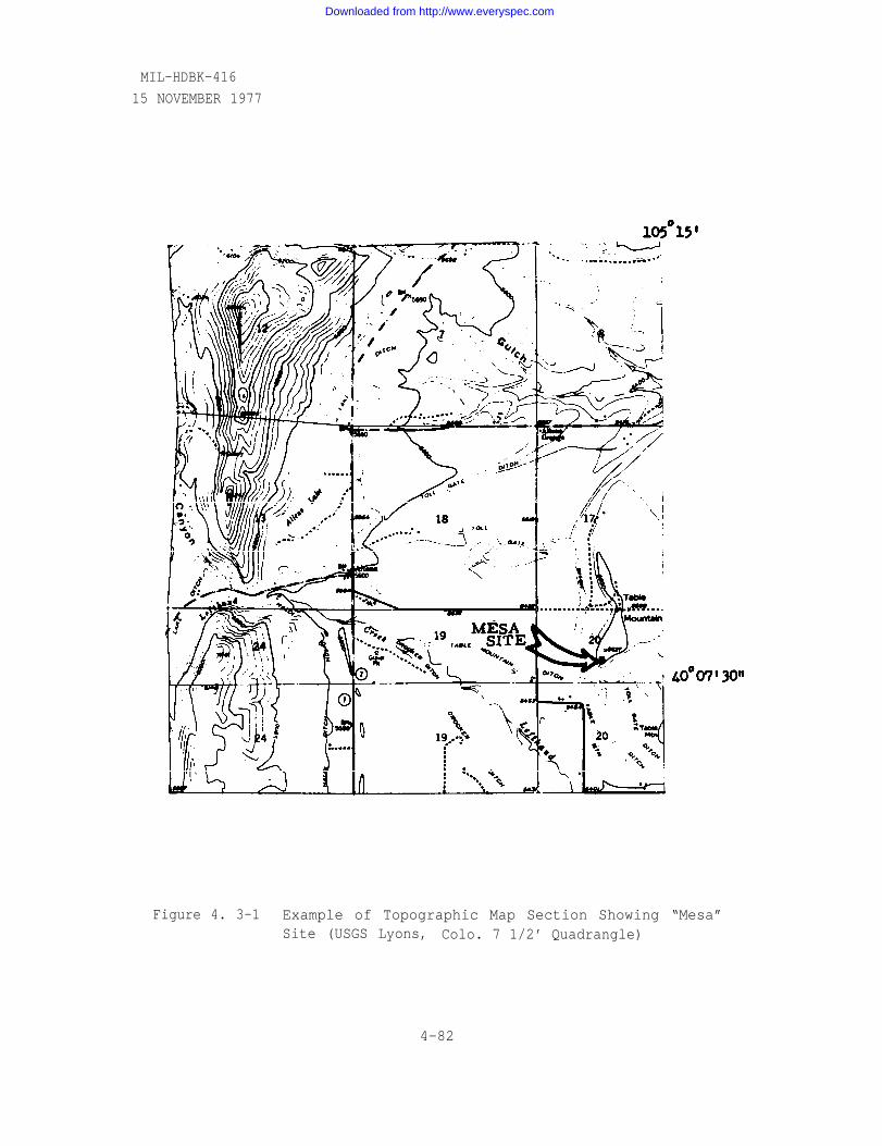
MIL-HDBK-416
15 NOVEMBER 1977
Figure 4. 3-1 Example of Topographic Map Section Showing “Mesa”Site (USGS Lyons, Colo. 7 1/2’ Quadrangle)
4-82
Downloaded from http://www.everyspec.com
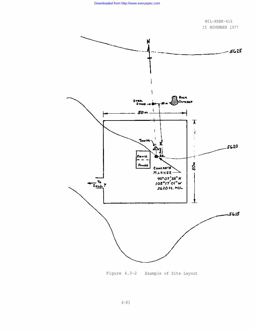
MIL-HDBK-416
15 NOVEMBER 1977
I
Figure 4.3-2 Example of Site Layout
4-83
Downloaded from http://www.everyspec.com

MIL-HDBK-41615 NOVEMBER 1977
A detailed topographic map of the site should be made
(fig. 4.3-2). Use photographs to show closeup details,
as well as general location with respect to surrounding
large-scale terrain features. For manned sites, an
estimate should be given of suitability with regard to
water supply and sewage disposal -- consult local Well
drillers, agricultural agents, plumbing contractors,
nearby farmers or ranchers. On the initial site visit,
general information on site location and access should
be summarized on a form similar to worksheet 4.3.2. This
will be useful in directing suppliers and contractors to
the site.
d. Description of path. Give general description
and vegetation as one proceeds along the path,
sible, from one site to the next; in particular,
of terrain
if pos-
check
elevations of ground and height of trees or buildings at
critical points. Distances should be determined to an
accuracy of ±0.1 mile (±0.2 km), azimuths to 1 minuteo
of arc, elevations to ±1 from path centerline. At crit-
ical points, obtain elevations within a radius of about
30 meters. Show by sketch and photographs new
construction or other features not correctly indicated by
available topographic maps. Make sketches and photo-
graphs on path centerline from each site, and show
azimuth angles to prominent features; also list elevation
angles. (Example: “Repeater #2 to repeater #3; start
survey at 0845 CST at BM #21A at site 2. Low rolling
grass-covered hills near site, crossing Big Sandy
Creek (20-ft wide)) at 6.8 miles; steeply rising terrain
.
4-84
Downloaded from http://www.everyspec.com
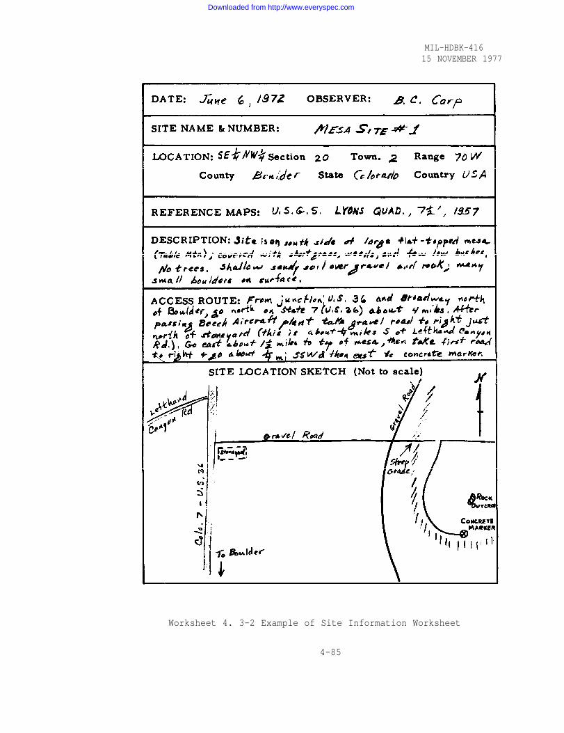
MIL-HDBK-41615 NOVEMBER 1977
Worksheet 4. 3-2 Example of Site Information Worksheet
4-85
Downloaded from http://www.everyspec.com
MIL-HDBK-41615 NOVEMBER 1977
e.
f.
g.
h.
i.
j.
beyond creek. Critical point at 7.9 miles, profile
shows 660 ft MSL, measured 672 ft by altimeter
#2167 at 0910 CST 11-10-72. Trees on critical point
ridge estimated 40 ft maximum by A bney level; beyond
critical point to site 3 is rough pine-covered hills.
150 ft water tower nearing completion approximately
500 ft west of path and 0.5 mile from site 2". )
Power availability. Give location of nearest commercial
transmission line with reference to each site; list name
and address of utility firm; state voltages, phase,
frequency, and main feeder size.
Fuel supply. List of local sources of propane, diesel
fuel, heating oils, natural gas; also estimate of cost of
item delivered to site.
Local materials and contractors. Determine if there
are local sources of lumber and ready-mixed concrete;
list names of local general contractors.
Local zoning restrictions. Make inquiry as to any that
might affect use of site or height of antenna tower. Give
distance from each site to nearest airport; determine if
site is in a runway approach corridor.
Geologic and seismic data. Determine load- bearing
qualities of soil at site, depth to rock and groundwater.
Obtain soil samples if appropriate. Check with local
authorities on the frequency and severity of seismic
disturbances.
Weather data. General climatological data
been assembled for the design studies, but
ologists can provide valuable supplemental
4-86
will have
local meteor-
details on
Downloaded from http://www.everyspec.com

the local variations of winds, temperatures, snow pack,
precipitation, cloudiness, fog, etc. , with reference to
hills, mountains, lakes, swamps, etc. , in the vicinity of
the sites. Check at local military and civilian weather
offices as to suitability of previous estimates for each
site, including,
(1) average maximum and minimum temperature
(monthly);
(2) average monthly precipitation, and extreme
short-period totals (day, hour), days/month
with rain;
(3) average wind direction and velocity, direction
and velocity of peak gusts;
(4) average and extreme snow pack;
(5) flooding possibilities;
(6) occurrence of hurricanes, typhoons, tornadoes;
(7) persistence of fog or low cloudiness;
(8) probability of extended periods of very light
winds;
(9) icing probability (freezing rain);
(10) average dewpoint temperature; diurnal variation
of relative humidity.
k. Other microwave systems or radars. Indicate on map
locations where “foreign” systems parallel or cross
the proposed route; show approximate locations of the
foreign repeater sites and name of operating agency.
Show location of radars, and determine power, wave-
length, and angle of coverage. TO ascertain the ambient
RF environment, electromagnet c radiation field surveys
may be conducted (see paragraph 4.2.22.4).4-87
M I L-HDBK-416
15 NOVEMBER 1977
Downloaded from http://www.everyspec.com

MIL-HDBK-41615 NOVEMBER 1977
k. Path loss data. These will only rarely be required;
see section 4.3.18 for further discussion.
4.3.4 Survey Equipment Requirements
4.3.4.1 Equipment necessary for the field survey will vary with the
demands of the design study, as well as with the type of terrain and
climate. In remote areas backup units should be taken for all major
equipment items, but this will not be necessary where supply depots are
relatively near. Each survey. will need to be considered separately to
assess the effects of loss of certain items of equipment.
4.3.4.2 Clothing, emergency shelter, and food supplies must be
adequate for the most adverse conditions, allowing for the possibility
of vehicle breakdown, road blockage, flooding, severe storms, etc.
Climatological data obtained from military or civilian sources should
be used in this planning.
4.3.4.3 Technical supplies and equipment will vary somewhat with the
type of survey; the following items are recommended:
a.
b.
c.
d.
e.
f.
g.
h.
i.
topographic maps, county road maps, path profiles,
plan of proposed site,
benchmark information from U. S. G. S. or other sources,
surveyor’s compass,
transit or theodolite (e.g., K & E or Wild) with laser
light filter,
tripod and leveling rod,
sensitive altimeter (preferably three each; e.g.,
Wallace & Tiernan FA-181), with psychrometer kit,
hand level- clinometer (e. g., Abney),
steel surveyor’s tape, 100 ft,
binoculars (7x35 or 8x50) with laser light filter,
4-88
Downloaded from http://www.everyspec.com

MIL-HDBK-41615 NOVEMBER 1977
j.
k.
l.
m.
n.
o.
P.
q.
r.
surveying handbook, ephemeris for current year,
wooden stakes, hammer) stake bag, ax or hatchet,
Polaroid camera and ample film supply,
field notebooks, protractor, rulers, dividers, clip-
boards, pencils, erasers, small hand tools, flash lights,
slide rule, small electronic calculator, math tables,
laser source with collimator, xenon strobotron light,
first-aid and snakebite kits,
several accurate watches; stop watch; small HF radio
for monitoring standard time broadcasts,
one of the microwave distance measuring devices (e.g.,
electrotype or tellurometer). These devices may be
adapted and calibrated for making certain types of path
loss measurements.
4.3.4.4 Two-way portable radios are indispensible in path surveys,
and also provide additional safety margin for work in remote areas or
under severe weather conditions. On long trips a supply of spare
batteries should be carried.
4.3.4.5 In areas with few benchmarks, a recording altimeter or
micro barograph can be used to improve the accuracy of the survey.
4.3.4.6 If soil sampling is required, a shovel, auger, and sample
containers should be included in the survey party supplies.
4.3.4.7 Path-loss measurements are not always required, but involve
sizeable quantities of additional equipment. See section 4.3.17.
4. 3.5 Transportation
4.3.5.1 In areas with a good road network, a station wagon is a
good choice for field survey transportation: tripods, leveling
rods, and instruments are protected from sun and weather and are
4-89
Downloaded from http://www.everyspec.com

MIL-HDBK-41615 NOVEMBER 1977
easily loaded and unloaded. In rough terrain, marshy areas, or where
roads are poor, a 4-wheel drive vehicle is recommended. Most sur-
veys will require at least two vehicles, and more will be necessary if
the survey is to include path-loss testing. In some areas it may be
more efficient to use a helicopter for site visits, particularly if sites
are a long distance from roads.
4.3.6 Personnel
4.3.6.1 The survey party chief should be a member of the system
design group who is familiar with the design objectives and has previous
experience in field surveys. Other members of the party should be
chosen on the basis of the particular needs of the survey; usually it
will be advantageous to select individuals with varying backgrounds
skills if they are available. For example, various phases of most
and
surveys can most suitably be performed by persons with experience in
communications engineering, surveying, civil engineering, meteorology,
and geology. Most tasks are such that more than one person is required.
For final surveys, however, the survey party should include at least
two well-trained and experienced surveyors. Where appropriate, the
survey party may also include representatives of local commands, host
countries, and contractors.
4.3.7 Frequency Requirements
4.3.7.1 If the path loss tests are to be performed, it will be neces-
sary to obtain authorization for use of the desired frequencies on the
particular paths. Permits may also be required for the mobile or
portable 2-way radios, and for electronic distance-measuring equip-
ment.
4-90
Downloaded from http://www.everyspec.com

MIL-HDBK-41615 NOVEMBER 1977
4.3.8 Time Requirements
4.3.8.1 The time required for the survey effort will include the time
required to assemble and brief personnel, procure and test equipment,
obtain permission for site visits, make the field measurements, and
assemble the data in a form suitable for use in the final stages of the
system design. Time estimates for field work should consider the
nature of the terrain, quality of roads, and weather conditions that may
be encountered. Ample time should be allowed for the site visits and
path checks; accurate information from these tasks is of greater con-
cern than early completion of the survey.
4.3.8.2 The path loss measurements team should be able to operate
independently, i.e., the rest of the survey team should not be required
to remain at a site or area while path loss measurements are in
progress.
4.3.9 Request for Survey
4.3.9.1 The necessary requests for manpower and equipment should
be initiated as soon as an estimate can be made of the completion date
for the route alternatives study. Consideration should be given to
climatic factors in areas where certain times of year are generally
unsuitable for field work.
4.3.10 Obtain Permission for Site Visits
4.3.10.1 As soon as sites have been selected, brief descriptions
of the sites should be prepared from the map data available, and perti-
nent information shown on accompanying sketch maps of each site.
These descriptions should be forwarded to the appropriate military
office with a request for site visit negotiations. The request should
describe briefly the purpose of the proposed microwave system, approx-
imate size of towers and buildings that may be necessary at each site,
4-91
Downloaded from http://www.everyspec.com

MIL-HDBK-41615 NOVEMBER 1977
and should outline specifically what the survey party plans to do at the
sites; e. g., set up theodolite, make distance and elevation measure-
ments, mark tentative tower location and site boundaries with stakes,
take soil samples (specify size), erect temporary tower for path loss
tests, etc. If any permanent defacement of the property is planned
(soil samples could be so considered) it should be plainly outlined in
the proposal for visit. Size and type of vehicles to be operated on the
site should also be given, as well as the maximum duration of the sur-
vey at each site, and the approximate calendar period in which the
survey will be made.
4.3.10.2 A copy of the complete set of site visit authorizations must
accompany the survey team. When a site is on private property, such
as a farm or ranch, it is recommended that the survey party visit the
owner or his tenant immediately prior to entering the site for the surve
Inquire as to preferred routes across the property (this may vary with
crop development), movement of livestock, etc. This courtesy may
influence later negotiations for lease or purchase of the site.
4.3.10.3 System design or field survey personnel will not ordinarily
participate in site visit negotiations, but should be prepared to furnish
a representative to accompany legal or property officers on visits to
property owners. Negotiating officers should be thoroughly briefed on
the purpose and general operation of the proposed system, so that they
will be prepared to answer questions on possible effects such as inter-
ference to radio or TV reception, health hazards from radiation, etc.
4.3.10.4 If there is a short time schedule for implementation of the
system, it may be desirable to proceed with land acquisition at the
same time permission for site visits is being arranged, i. e., options
for lease or purchase should be negotiated.
Y.
4-92
Downloaded from http://www.everyspec.com

MIL-HDBK-41615 NOVEMBER 1977
4.3.11 Site Visits
4.3.11.1 Upon arrival at a site, the first task of the survey team will
be to verify the location selected on the basis of the map studies.
There are likely to be small variations in the topography that were not
shown on the maps, and it may be desirable, in the judgment of the“
survey chief, to make small adjustments in the site location. The
permanent site reference markers should then be placed and surveyed
in. Next, the location of the antenna tower and buildings should be
marked by stakes in accordance with the preliminary site plan. From
the location of the tower and buildings, the boundaries of the desired
plot of land should then be determined and marked by stakes, taking
into consideration the tentative location of anchors for guyed towers
if they are to be considered.
4.3.11.2 A sketch of the site is made in a field notebook, showing the
location of the tower and buildings, trees, large boulders, ditches,
etc. Then measurements are made with the steel tape, and recorded
with dimension lines on the sketch, so that an accurate site map can
be prepared. The sketch should be clearly identified by name, site
number, geographical coordinates, and quadrangle map name or
number. It should be accompanied by a verbal description of the type
of soil, vegetation, number and size of trees (trunk diameter and
height), number of trees that will have to be removed, approximate
location and extent of leveling required. If soil samples are required,
the sampling points should be marked on the site sketch.
4.3.11.3 Photographs are made of the horizon to the north, east,
south, and west from the tower location, and also along the centerline
of each path from the site; these should be fully identified and fastened
to a page in the notebook. Use a transit or theodolite to determine
azimuths of prominent features on the horizon of each photograph, and
4-93
Downloaded from http://www.everyspec.com

also indicate the elevation angle to prominent features of the path-
centerline photographs. If possible, photographs should also be made
at a short distance from the site to provide an overall view of the entire
site; site boundaries and tower location should be entered on these in
ink. A more distant view, to show the site area with reference to
surrounding major terrain features, will also be useful.
4.3.11.4 Generally speaking, azimuths determined by magnetic compass
are not sufficiently accurate for radio path surveys. When the compass
is used for rough orientation, it should be corrected for the local declin-
ation, which may be obtained from topographic or aeronautical charts.
There are, however, irregular or local variations of the compass bearings
that are caused by magnetic storms, iron ore deposits, large objects of
iron or steel, and electric power lines; therefore great caution must be
used in checking site or path azimuths with a compass, particularly in the
far north (e.g., Alaska, Iceland, Greenland) or in areas with known large
mineral deposits. Azimuth references should be determined or con-
firmed by celestial observations if possible (see section 6.1).
4.3.11.5 The latitude and longitude of the tower location on the site
should be determined to ±1 second. This can be done by map scaling,
traverse survey, triangulation survey, and celestial observations. The
method selected may vary with the particular conditions, such as ir-
regular terrain and distance from a benchmark. In most cases this
accuracy can be attained by careful scaling from a 7 1/2 minute quad-
rangle with a device such as the Gerber Variable Scale (one second of
latitude = 101 ft or 31 meters, approximately). It will rarely be neces-
sary to determine location by celestial observations, which require
considerable time, highly skilled observers, and good instruments.
The location should also be described with reference to nearby roads
and cities so that contractors and suppliers can be readily directed to
the site as indicated on the example in worksheet 4.3-2.
4-94
MIL-HDBK-41615 NOVEMBER 1977
Downloaded from http://www.everyspec.com
MIL-HDBK-41615 NOVEMBER 1977
4.3.11.6 The elevation of the ground at the tower location should be
determined to ±1.5 meters. The method used depends on field condi-
tions, distance to benchmarks, personnel and equipment available, and
type of survey. Differential leveling, or the extention of a known verti-
cal control point (benchmark) by a series of instrument setups, is the
most accurate method and is recommended for the final survey or when
there is a benchmark close to the site. Trigonometric leveling is use-
ful where elevations must be determined over relatively long distances,
as in very irregular or inaccessible terrain; it is not ordinarily used
for site surveys but may be employed to determine the elevation of
obstacles along a radio path. Aerial photogrammetry and airborne
profile recorders (radar or laser) can also be used, although these
techniques tend to be quite expensive. Barometric leveling (or survey-
ing altimetry) is the simplest method of determining relative ground
elevations, and is particularly useful for initial surveys, although it
can also provide the accuracy required for the final survey by careful
use. Barometric techniques are treated in detail in section 4.3.13
and section 6.2.
4.3.11.7 For the initial survey, prepare a site sketch map similar to
figure 4.3-2; include coordinates, location of prominent objects, eleva-
tion data, etc., using a scale on the order of 1" = 10 to 50 ft and contour
intervals of 1 to 5 ft; it should show location of the reference baseline,
nearby benchmarks, tower and building locations, etc. The preferred
method of establishing the reference baseline is by celestial observa-
tions (see section 6.1).
4.3.11.8 The access to the site must be described in detail so that
estimates can be made of the cost of building a road to the site. Pre-
pare a sketch map showing the route of the proposed road with reference
to the site and existing roads; also indicate the type of soil, number of
4-95
Downloaded from http://www.everyspec.com

MIL-HDBK-41615 NOVEMBER 1977
trees that will probably have to be removed, degree of slope, and
approximate length of the road (as compared to the most direct distance
from the site to existing roads).
4.3.11.9 The probability of all-year access to the site should be esti-
mated after discussing the matter with nearby residents, highway
department maintenance personnel, and local meteorologists. Get an
estimate of the number of days per year when existing roads in the
area are impassable because of snow conditions or heavy rains. In-
quire as to the possibility of snow removal and regular maintenance by
highway department crews and equipment.
4.3.11.10 The availability of commercial electric power will be a
major factor in determining the operating expenses of the site. If
there is a nearby transmission line show its approximate route on a
topographic or road map as well as recording pertinent details in the
field notebook. Obtain the name and address of the utility company,
and make inquiry as to the existing policy on line extensions for new
customers. The survey party should have available information on the
approximate power requirements of the repeater or terminal radio
equipment, size and type of construction of the equipment buildings,
and temperature to be maintained by air conditioning, so that utility
officials can estimate the overall site power demands.
4.3.11.11 If the site is in an area where heating of the building will be
necessary, determine if there are local sources of propane, natural
gas, or heating oils. Also check on availability of fuel for the standby
motor-generator. Determine approximate costs of these items, de-
livered to the site.
4.3.11.12 List nearest sources of building materials, such as lumber
brick, concrete blocks, ready-mixed concretes List local general,
electrical, and heating contractors.
4-96
Downloaded from http://www.everyspec.com

MIL-HDBK-41615 NOVEMBER 1977
4.3.11.13 Check with local authorities on possible zoning restrictions
in the site areas regarding type of construction permitted, require-
ments for sanitary facilities, maximum height limitations, etc. Also
check locations of nearby airports to see if proposed site is in the
approach corridor of any of the runways.
4.3.11.14 Depending upon the nature of the proposed site, it may be
necessary to check the depth of groundwater and bedrock and obtain a
local opinion on the load-bearing qualities of the soil at the site. In
some areas, it will be appropriate to check with local sources of infor-
mation on the frequency and severity of seismic disturbances.
4.3.11.15 Weather conditions should be discussed with local meteor-
ologists, as outlined in 4.3.3.3j.
4.3.11.16 The site visit also affords an opportunity to verify the exist-
ence, locations, and operational data of any other communications or
radar terminals as noted in 4.3.303k.
4.3.11.17 Path loss testing is rarely required on LOS paths. If per-
formed by a team independent of the survey party, it will be important
that the exact locations selected for the antennas by the survey party be
used in setting up antennas and towers for the path loss tests. Test
procedures are further discussed in section 4.3.20.
4.3.11.18 Interference measurements may be required on some sites,
depending upon what is already known or learned during the field survey
about possible interference sources. Microwave repeaters should not
be located less than 10 miles from a radar. If possible, terrain shield-
ing of potential line-of-sight paths between the repeater and any radars
up to 50 miles distance should exist under all conditions (even when
ducting occurs). Interference may also result from other microwave
systems that parallel or intersect the proposed system [4].
4-97
Downloaded from http://www.everyspec.com

MIL-HDBK-416
15 NOVEMBER 1977
4.3.12 Survey Terrain Clearances
4.3.12.1 When the site visit tasks have been completed at both ends of
a radio path, the terrain clearances should be checked, and other
pertinent information on the path recorded. There will usually be only
a few points on the radio path where clearance is critical, however, the
entire path profile needs to be verified to some extent by the survey
party. The maps available for design studies are frequently several
years old, and recently constructed buildings, reservoirs, storage
tanks, and roads may alter the map indications of clearances, reflec-
tion points, and site access. Any changes noted should be entered on
the topographic maps, the terrain profile and in the field notebook;
large structures should be photographed and the approximate dimensions
shown on the photographs. A description of the terrain and vegetation,
as one proceeds from one site to the other, is also entered in the field
notebook (see example 4.3.3.3d).
4.3.12.2 Normally, conventional techniques involving differential
leveling or precision altimetry will be used to check the terrain clear-
ances. Other methods that may be useful in some circumstances in-
clude optical surveys (use of laser source, mirrors, and theodolites),
airborne radar profile recorders, and three-dimensional aerial photog-
raphy (photogrammetric techniques). The latter two tend to be relative -
ly quick, but do not eliminate the need for site visits. In certain
cases, however, they may provide information that could not readily be
obtained by other methods.
4.3.12.3 The advantages and disadvantages of various terrain-
checking techniques are as follows:
4.3.13 Profiles from Altimeter Surveys
4.3.13.1 Altimeter surveys are used to check elevations of critical
points, especially in rough country or where existing maps are poor.
4-98
Downloaded from http://www.everyspec.com

MIL-HDBK-41615 NOVEMBER 1977
The type of terrain to be covered will have a direct bearing on the
cost, accuracy and the time taken to complete the survey. Rugged,
inaccessible country will make it very difficult to obtain good results,
for the following reasons:
a. it is difficult to locate a point on the ground as being
directly on the radio path. Hence, it must be assumed
that the highest point in the immediate area will form
the obstruction,
obstructions may be difficult to reach by parties on foot;
c. the accuracy of the survey depends largely on the time
required to make comparative altimeter readings at
different locations. The longer this interval, the great-
er the chance of a change in temperature or barometric
pressure that could cause an error (see section 6.2).
The use of helicopters can shorten these time intervals,
from hours to minutes, particularly if the survey route
requires scaling of difficult peaks. This saving in time
can sometimes offset the expense of the helicopter, and
this may even be more important on urgent jobs.
4.3.13.2 The methods of conducting altimeter surveys are covered in
surveying textbooks [94, 96] and in the manuals distributed by makers
of surveying altimeters. The accuracy obtainable is usually adequate
if the survey is made by experienced personnel using good equipment.
4.3.13.3 Section 6.2 contains a summary of meteorological factors
that can affect the accuracy of altimeter surveys, lists precautions to
be observed in the use of altimeters, and describes techniques for using
the altimeter on radio path surveys. Additional details can also be
found in T.O. 31R5-1-9 [10].
4-99
b.
Downloaded from http://www.everyspec.com

MIL-HDBK-41615 NOVEMBER 1977
4.3.14 Profiles from Optical Surveys
4.3.14.1 Optical methods of checking obstructions on radio paths are
discussed in detail in section 6.3.Light from xenon tubes or sunlight
from mirrors are used in conjunction with theodolites. These methods
are used to measure the locations of obstructions as well as vertical
angles to determine elevation differences.The discussion in section
6.3 includes an evaluation of the relative accuracy of the various
methods,
involved.
4.3.15
4.3.15.1
Recorder
and numerical examples with sketches of the geometry
Profiles from Aerial Surveys
Profiles can also be obtained by using a Terrain Profile
(TPR) on aerial surveys of the proposed routes. The TPR
system consists of a precision radar altimeter, a pressure sensing
device called a hypsometer, and a continuous-strip 35 mm camera,
which has been bore-sighted to the axis of the radar beam. The hypso-
meter measures the aircraft deviation from a preselected barometric
altitude, while the radar altimeter measures the terrain clearance.
The continuous-strip camera is set to take overlapping photographs to
record the exact aircraft position; the recorded data include the trip -
ping time of each exposure, the indication of the aircraft and radar
altimeters, and the deviation shown by the hypsometer. A similar
system employs a laser altimeter instead of the radar altimeter;
ever, this system has an operational limit of about 6000 ft, while
system with the radar altimeter can be employed from about 6000
32000 ft.
4.3.15.2 Path profiles can be obtained quickly by aerial methods, but
there are a number of potential sources of error. These include the
following:
how-
the
to
4-100
Downloaded from http://www.everyspec.com

MIL-HDBK-41615 NOVEMBER 1977
a.
b.
c.
d.
e.
Determination of the radio path center line -- the pilot
needs markers and checkpoints, but these may be diffi-
cult to provide in rugged or inaccessible terrain, and
may be of questionable accuracy if available maps are
poor.
Beamwidth -- the radar beamwidth will vary from 100 to
500 ft at the surface, depending upon the altitude of the
aircraft. Since the recorded signal corresponds to the
high point in this strip, the indicated elevation of the
radio path could be considerably in error in rough
terrain.
The radar beam penetrates foliage of trees to a variable
and unknown degree.
The effects of thermal or mechanical turbulence and
wind drift make it difficult to hold a precise course and
altitude, and any tilt of the radar beam causes errors in
the “on-course” elevations.
General errors in pressure altimetry are discussed in
section 6.2. These include instrumental lag, tempera-
ture errors, and errors related to movement of pressure
systems. Sizeable errors may occur in the vicinity of
thunderstorms, where “pressure jumps” frequently
occur. In addition, there are errors related to the
static pressure system of aircraft altimeters.
4.3.16 Profiles from New Maps Drawn from Aerial Photographs
4.3.16.1 Profiles may be obtained from maps based on three-
dimensional aerial photographs, using photogrammetric techniques.
Very high accuracy is possible if a sufficient number of precise ground
4-101
Downloaded from http://www.everyspec.com

MIL-HDBK-41615 NOVEMBER 1977
control points are used. A series of photographs is made of the desired
area from altitudes between about 300 m and 10,000 m, depending on
the scale and accuracy required. Each photograph has a 60% overlap
with adjacent photographs, and a set of two adjacent pictures forms a
“stereo pair” that gives a three-dimensional model of the terrain, when
seen through a special viewer/plotter device. This has a measuring
system for determining horizontal and vertical distances from the
projected model by reference to the photo control points previously
surveyed and marked on the ground. Auxiliary equipment can be set to
trace a particular elevation and plot the contour lines over the area to
the desired interval.
4.3.16.2 The comparative cost of this method and more conventional
techniques of preparing path profiles is not known at present. It is
doubtful if photogrammetric methods would be economically feasible for
single links, but for an extensive system the costs should be more
competitive. If recent photographs are available, photogrammetric
techniques may provide much more current path information than could
be obtained from the best available topographic charts, which may be
several years old, and may not show recent changes on the radio path
that could significantly influence path performance such as new construc-
tion, or perhaps the highly reflecting surface of a new reservoir.
Interpretation of the stereo photographs by experts can also provide
information on the type, height, and density of trees, as well as the
best location for access roads, sources of water supply, location of
power lines, and sources of possible interference.
4.3.17 Path Loss Measurements
4.3.17.1 Path loss tests, if required, are made by transmitting an un-
modulated RF carrier between adjacent repeater sites and measuring
4-102
Downloaded from http://www.everyspec.com

MIL-HDBK-41615 NOVEMBER 1977
the received power levels over a period of time and in some cases for
various combinations of antenna elevations. Path loss as a function of
time and antenna height is readily determined from such data if trans-
mitter power, antenna gains, and waveguide losses are known.
4.3.17.2 Path loss measurements are not usually necessary on care-
fully designed LOS radio links. There are paths, however, where it
may be advisable to make such tests prior to facility construction. If,
for example, antennas of the heavy horn-reflector type are to be used,
the antenna position on the tower cannot easily be changed once the
installation is completed. In such cases height-gain measurements
may help in determining the optimum antenna position. Measurements
are also recommended on any path where there is a possibility of strong
ground reflections, or on paths where design calculations indicate
borderline conditions of fading margin or Fresnel-zone clearance (see
section 4.2). These problems might arise where the choice of suitable
sites is limited, or local zoning restricts tower heights (near airports,
as an example).
4.3.17.3 Manpower and equipment required for path loss testing make
it an expensive operation. Temporary towers are usually required at
both sites as are some means of moving the antenna quickly from one
position on the tower to another (a clamp-on track is sometimes used).
Portable power units will also be needed, in addition to a stable trans-
mitter and receiver, recording equipment, transmission lines, and
calibration equipment. The tests must be made over exactly the same
path as that intended for the final installation, and in rough or heavily
wooded terrain it may be nearly impossible to make measurements
until the sites have been acquired, ground cleared, and access roads
provided.
4-103
Downloaded from http://www.everyspec.com

MIL-HDBK-41615 NOVEMBER 1977
4.3.17.4 Section 6.4 contains more detailed information on the desir-
able equipment and tower characteristics for path loss testing, as well
as suggestions relative to calibrations and operational procedures.
4.3.18 Objectives of Path Loss Tests.
4.3.18.1 Since the performance of path l0SS tests may become quite
expensive and require a substantial amount of time, a careful analysis
of test objectives must be made before a field effort is mounted. Such
an analysis is logically based on the results of the preliminary design
work described in section 4.2 (Study of Route Alternatives). In general,
path loss tests on line-of-sight links may have the following objectives:
a. Verification of line-of-sight conditions over a specific
link,
b. to provide a basis for selecting optimum antenna heights,
c. evaluation of potential fading phenomena, and basis for
selecting antenna spacings for diversity operation.
4.3.18.2 Since line-of-sight systems are usually designed with ade-
quate terrain clearance, as discussed in section 4.2, verification of
line-of-sight conditions by path loss measurements may only be re-
quired on long links where the information from available maps is not
reliable, and optical methods cannot be employed. Other considerations
and procedures to achieve the three objectives will be discussed in the
following paragraphs.
4.3.19 Antenna Height Gain, Lobing, and Atmospheric Effects.
4.3.19.1 If we assume a link over relatively smooth ground where a
single specular reflection can be obtained, the relative phase of the
direct and the ground-reflected component changes with antenna height
and produces alternative addition and cancellation in the resultant field
at the antenna. Starting with heights corresponding to grazing, the
4-104
Downloaded from http://www.everyspec.com

MIL-HDBK-41615 NOVEMBER 1977
resultant field will first rise rapidly to a maximum with increasing
antenna height, and then will go through a series of “lobes” (i.e., the
successive maxima and minima) when the height is increased further.
These lobes become smaller with increasing antenna height; i.e., the
maxima and minima are closer and closer together until they are no
more distinguishable because of the integrating effect of the antenna
aperture. The spacing between maxima and minima is also a function
of carrier frequency.
4.3.19.2 The lobing pattern as a function of height for the case just
discussed will also change as a function of changes in the atmospheric
refractivity gradient, and complex patterns may result from a sharply
stratified atmosphere which may produce atmospheric multipath compo-
nents in addition to the ground-reflections previously discussed.
4.3.19.3 If there are no ground reflections, no lobing pattern will be
observed and the received field will rise with antenna height to the
free-space value and remain essentially constant for further height
increases. Such a condition will usually exist in practice where the
terrain is sufficiently irregular to prevent specular reflections, partic-
ularly at higher microwave frequencies. Occasionally, multiple
specular ground reflections will occur and may complicate the lobing
pattern in a manner similar to atmospheric multipath.
4.3.20 Verification of Line-of-Sight Conditions.
4.3.20.1 Based on the discussion in paragraph 4.3.17.3 above, the exist-
ence of line-of-sight conditions can be quickly verified, if required, by
measuring the received power over a specific link for a short time,
and comparing the measured level to that corresponding to free-spice
propagation conditions. This should be done preferably at times when
the atmosphere is well-mixed so that effects of stratification do not
4-105
Downloaded from http://www.everyspec.com

MIL-HDBK-41615 NOVEMBER 1977
appear. Considering atmospheric absorption over the path (see section
4.2.22) and possible calibration errors, the received power level over
line-of-sight links up to about 50 km in length should be within a few
decibels of the free-space value.
4.3.20.2 If the test antenna at one of the terminals can be raised and
lowered, an assessment of potential fading conditions can be made in
many cases. If a substantial lobing pattern exists even under conditions
of a well-mixed “standard” atmosphere, multipath propagation by
reflections from terrain can be assumed to exist. Since the lobing
pattern, as already noted, changes with atmospheric characteristics,
substantial fading can be expected, and the use of diversity operation
over the link should be considered.
4.3.20.3 A recent CCIT Handbook ([12], see appendix to section
B.IV.3, section 14) includes suggested test procedures to determine
the location of obstructions and values of the effective earth radius
factor, k, from path l0SS measurements. However, these procedures
are largely based on idealized terrain and atmospheric conditions; e.g.,
specular reflections from well-defined portions of the terrain along the
path, and a well-mixed atmosphere with refractivity gradients which
may be time-varying, but are constant over the volume of the propaga-
tion path at any particular time. Consequently, it is not likely that
such tests will produce unique results in a cost-effective manner.
4.3.21 Selecting Optimum Antenna Heights by Path Loss Tests.
4.3.21.1 Raising and lowering an antenna may prove or disprove the
existence of a lobing pattern for the specific atmospheric conditions
existing at the time of the tests, but it should not be attempted to fix or
recommend a particular antenna height on the basis of a short-term
test. This is particularly applicable to cases where the frequency for
4-106
Downloaded from http://www.everyspec.com

MIL-HDBK-41615 NOVEMBER 1977
path loss tests is not the same as that which will be ultimately used for
the system, since the lobing pattern is frequency-dependent.
4.3.21.2 If antenna heights must be determined or verified by path
loss tests over a short time period, they should be selected in the mid-
dle of a height interval within which the received field is close to the
free-space value and constant within a few decibels. This will provide
some assurance that day-to-day changes in the average atmospheric
refractivity will have no appreciable effects on the received radio
frequency power.
4.3.21.3 Positioning the antenna within a height region where the
received field varies rapidly with height should be avoided. A mono-
tonic increase in field of tens of decibels over antenna height increases
of several meters is a good indication that the path is close to grazing
and may be subject to blocking and resulting power fading during sub-
refractive conditions (see section 4.4.11). Figure 4.3-3 is a pictorial
representation of possible field strength variations with antenna height
for a well-mixed atmosphere, and includes suggestions for “good” and
“bad” antenna positions. However, greater confidence in determining
antenna position can only be obtained from a combination of careful
analysis of path geometry and available refractivity data with long-
term simultaneous measurements at several heights. Such a proce-
dure is usually too expensive in relation to benefits derived for most
practical microwave links.
4.3.22 Evaluation of Fading Phenomena and Diversity Design.
4.3.22.1 There are systems and links where it is not possible for a
number of reasons to employ sufficient antenna heights to provide ade-
quate terrain clearance, or where paths are exceptionally long, or
where climatological conditions are conducive to severe fading.
4-107
Downloaded from http://www.everyspec.com

MIL-HDBK-41615 NOVEMBER 1977
Figure 4.3-3 Example of field strength variations with antennaheight for a well-mixed atmosphere.
4-108
Downloaded from http://www.everyspec.com
MIL-HDBK-41615 NOVEMBER 1977
Examples are primarily paths over water with limited tower heights.
Since it has not yet been possible to deduce statistics of the expected
received power levels from a limited knowledge of the statistics of
atmospheric characteristics, it may in some cases be useful to perform
path loss measurements over an extended period of time in order to
obtain more confidence in the performance predictions, or even to
avoid costly overdesign.
4.3.22.2 Path loss tests under such circumstances may be performed
using the equipment installed and operating on the basis of best avail-
able design estimates in accordance with the material in sections 4.2
and 4.4. However, the results of the tests may indicate desired
changes in the equipments antenna positions, and diversity design. It
will usually be advantageous to select periods for path loss tests when
severe fading is anticipated.
4.3.22.3 Available meteorological data should be consulted to deter-
mine diurnal and seasonal periods when atmospheric stratification and
ducting is likely to exist. As an example, this may correspond to
summer nights for paths over flat terrain in a temperate zone. For
overwater links, or links in coastal areas, the possibility of changes in
refractivity gradients related to seasonal shifts in the prevailing wind
flow should be considered. In one season the air flow may bring warm,
dry air from the land over the sea (a condition frequently causing radio
ducts), while in another season the flow may be predominantly from
sea to land. On the basis of such qualitative analyses the best season
and suitable daily schedules for path loss measurements can be
determined.
4.3.22.4 Simple criteria regarding diversity design (i.e., spacing of
antennas, or frequency separation) have been given in section 4.4.24.
However, these criteria may not be applicable in cases where
4-109
Downloaded from http://www.everyspec.com

pronounced lobing patterns due to specular reflections from the ground
exist, and where strong atmospheric stratification can be expected
during a large percentage of the time. Dougherty [35] has shown
methods to determine antenna separations in space, or frequency
separations which assure that the two channels of a diversity system
would not be subject to simultaneous fading for a wide range of possible
refractivity gradients. Path loss tests over a longer time period can
be used effectively to verify the usefulness of configurations deter-
mined in this manner from theoretical considerations. A discussion
of applicable measurement results for a long line-of-sight link in
moderately rolling country has been presented in [97].
4.3.23
4.3.23.1
should be
Utilization of Survey and Measurement Data.
On conclusion of the field observations, the survey data
summarized for use in the final system design studies.
Most of the analysis and summarization of field data is best done while
the survey is in progress, since omissions or discrepancies noted can
then be readily checked while the survey party is still in the area.
Site maps should be prepared for each site, showing locations of anten-
nas, access roads, etc. Significant discrepancies between the original
path and site data should be listed, and corrections shown on path
profiles and topographic maps. A n information folder should be pre-
pared for each site, containing maps and all other pertinent informs-
tion, such as land ownership, power availability and cost, climatic
data, zoning restrictions, etc.
4.3.23.2 If path loss measurements were made, the records should
be analyzed and height-gain graphs plotted when applicable. Long-
term records should be carefully analyzed to obtain statistical informa-
tion regarding power levels, fading frequency and depth, and diversity
improvement.
4-110
MIL-HDBK-41615 NOVEMBER 1977
Downloaded from http://www.everyspec.com

MIL-HDBK-41615 NOVEMBER 1977
4.3.23.3 In using the various data collected by the survey party,
technical desirability must be weighed against site availability, cost of
leasing or purchasing land, site preparation and road access costs,
fuel and power costs, and all-year accessibility. Security considera-
tions may also become important in certain areas.
4.3.23.4 Requests forwarded to area commands for approval of sites
should be accompanied by maps and other detailed information, such as
legal description of the property, name and address of owner or legal
representative (see also worksheet 4.3.2).
4-111
Downloaded from http://www.everyspec.com

Section 4.4 LINK DESIGN.
4.4.1 General
4.4.1.1 Using Section 4.1, certain basic information about the
system was obtained: its geographic location, channel requirements,
and its location in the spectrum.
4.4.1.2
and how
order to
with site
4.4.1.3
accurate
Section 4.2 described selection of
to systematically grade the site and
select the more desirable ones for
surveys.
Section 4.3 described methods of
potential sites and routes,
route alternatives in
additional investigation
obtaining complete and
information needed for final selection of links and for provid-
ing detailed, accurate path profiles and site layouts. In addition,
explicit information about potential interference sources was obtained.
4.4.1.4 With this knowledge, we can proceed now in Section 4.4 to
describe how to check, analyze, and summarize the information
described in 4.1,4.2, and 4.3 and finally, we will consider how to
make a preliminary selection of equipment types and sizes for a
stated performance of each link in terms of median voice channel
signal-to-noise ratio. The discussion on adjustments of link design
resulting from system noise performance estimates will be presented
in Section 4.5 (see figure 4.5-14). The required median signal-to-
noise ratio for each link may be obtained from appropriate DCA
standards that are current at the time and the communication traffic
requirements information described in Section 4.1. Section 4.4
includes background information on propagation effects with emphasis
on fading mechanisms. It is organized as follows (see also figure
1-4):
4-112
MIL-HDBK-41615 NOVEMBER 1977
Downloaded from http://www.everyspec.com

a.
b.
c.
d.
e.
f.
MIL-HDBK-41615 NOVEMBER 1977
Path profile upgrading and checking (sect.4.4.3).
Calculating tower heights (sect. 4.4.4).
Propagation (sect. 4.4.5 through 4.4.21).
Diversity (sect. 4.4.22 through 4.4.25).
Radio frequency interference (sect. 4.4.26 through
4.4.27).
Equipment considerations (sect. 4.4.28 through 4.4.46).
4.4.2 The link design estimate
4.4.2.1 The worksheets in section 4.4.3 are used for summarizing
the results of the initial estimates of the link design as demonstrated
by the example. Because of the prodigious number of equipment
options, the large range of terrain and climate conditions, and the
variety of interference environments, no attempt has been made to
provide a totally self-contained
section 4.4. Final selection of
discussed in section 4.5
4.4.2.2 The basic link design
set of link design worksheets in
equipment types and sizes will be
information should be documented on works beets
4.4-1 through 4.4-5 as shown by the example given here and also in section
4.5.41. Reference is made on these worksheets to the various sections of the
handbook that will be helpful for obtaining desired pieces of information. The
last result on worksheet 4.4-5 (step 44) is the expected median receiver input
power, in dBm. As a first estimate, this value Pr is sufficient if it
exceeds the sum of the
receiver thermal noise
thermal noise level 10
figure F in dB. These
required median carrier-to-noise ratio (in dB) and the
threshold (usually in dB). The latter is the sum of the
log(kTBIF) (usually in dBm) and the receiver noise
terms are further defined in par. 4.5.27.2; it will
suffice for the present to state that the thermal noise level in dB can be ex-
pressed by(-174 + 10 log BIF) where the intermediate frequency bandwidth BIF is
in Hertz. Figure 4.4-1 is a example of required values of receiver input power4-113
Downloaded from http://www.everyspec.com

Figure 4.4-1
MIL-HDBK-41615 NOVEMBER 1977
4-114
Downloaded from http://www.everyspec.com

MIL-HDBK-41615 NOVEMBER 1977
for an FDM/FM system based on currently applicable DCS Standards [98], and may
be used for this purpose.
given in the legend; this
added to offset equipment
The curves in this figure are based on the equation
is equation (4.5-10) solved for Pr with a 3 dB term
noise. The IF filter bandwidth BIF is assumed to
be equal to the radio frequency bandwidth brf. For this example, the required
value of the voice channel signal-to-thermal noise ratio, S/Nt, is assumed to be
66 dB and the receiver noise figure is 10 dB. At the median value Pr of receiver
input power, equipment noise will probably be a substantial factor in determining
the voice channel signal-to-noise ratio; this is the reason for the added 3 dB
term as noted above.
4.4.3 Path profile upgrading and checking
4.4.3.1 In the initial stages of the design a path profile of the link
should have been plotted in accordance” with Section 4.2.15 and figure
4.2-4. Now, corrections corresponding to the information obtained
from the site survey should be incorporated into the profile, and it
should be checked to see if it contains the following pieces of information:
a.
b.
C.
Check the validity of the site coordinates marked on the
map from which the profile was plotted with those
obtained during the site survey.
The height above mean sea level of the terminal points
the profile should agree with the heights measured in
accordance with Section 4.3.11, and as shown for the
tower base height in figure 4.3-2.
on
The photographs taken in accordance with Section 4.3.11
should be checked for down-path clearance in the imme-
diate foreground, and the elevation angle to the horizon
indicated by the geometry of the profile should be checked
against the measured elevation angle down-path.
4-115
Downloaded from http://www.everyspec.com

MIL-HDBK-41615 NOVEMBER 1977
d .
e.
f.
g.
h.
If there are trees or buildings at the site and on or near
the center line down-path, make sure their heights and
locations are shown on the profile. For trees, an allow-
ance for
example
Indicate
profile.
indicate
growth should be indicated as shown in the
on Worksheet 4.4-1.
any local restrictions on tower heights on the
If the antenna tower already exists on site,
at what heights antennas can be placed.
Check that the results of the terrain clearance survey
described in Section 4.3.12 are incorporated in the
profile.
Make sure that potential specular reflectors mentioned
in the site survey data or shown on the map (such as
bodies of water which lie along the path) are noted on
the profile.
Make a check of the height of critical points along the
profile for agreement with the corresponding points on
the map used for the plotting of the profile.
4.4.3.2 If during the site survey enough information was obtained on
local weather data to estimate the range of refractive index gradients,
indicate this range on the profile (see also paragraph4.4.5.1)
4.4.3.3 Worksheets
The worksheets in this section show how to organize the terrain profile
and equipment information for an individual line-of-sight link, so that design
parameters can easily be summarized and tabulated. An appropriate example is
started on worksheet 4.4-1, 4.4-2 and 4.4-3; the complete link design calcula-
ions for this example are given on the filled-in worksheets in section 4.5.41
4-116
Downloaded from http://www.everyspec.com

MIL-HDBK-41615 NOVEMBER 1977
Notes:1. A 30 percent allowance for grouth has been
included in the tree heights shown on the profile.
2. The worst estimate of sub-refractive gradients
for this area is +39 N units/km corresponding
to a value of k=0.8 (Fig. 4.4-4)
3. The take-off angle, , at site No. 1 is determined
by Eq. 4.2-4. Since for k=4/3 (a=8493 km),
(h2-d2/2a) is less than h1, the angle of
penetration of potential layers at some location
along the path will be zero.
Worksheet 4.4-l Link Design Profile (Example)
4-117
Downloaded from http://www.everyspec.com
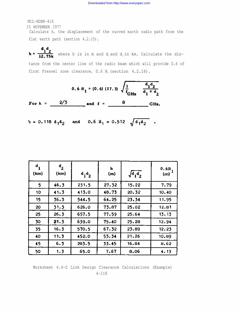
MIL-HDBK-41615 NOVEMBER 1977Calculate h, the displacement of the curved earth radio path from the
flat earth path (section 4.2.15).
where h is in m and dl and d2 in km. Calculate the dis-
tance from the center line of the radio beam which will provide 0.6 of
first Fresnel zone clearance, 0.6 R1 (section 4.2.18).
Worksheet 4.4-2 Link Design Clearance Calculations (Example)
4-118
Downloaded from http://www.everyspec.com

A. Distance on Profile 26.3 km.
Ground Elevation 390 m above m.s.l.
Tree or Obstacle Height 30 m above ground.
Total Obstruction Height 420 m above m.s.l.
For an assumed upper antenna height of 100 m & 100 m, clearance of
13.6 m is realized for “k” = 2/3 . This provides(worst case)
0.6 of First(fraction) (order)
Fresnel Zone clearance for this “k” value.
B. Distance on Profile km.
G round Elevation m above m.s.l.
Tree or Obstacle Height m above ground.
Total Obstruction Height m above m.s.l.
For an assumed upper antenna height of m, clearance of
m is realized for “k” = . This provides(worst case)
of Fresnel Zone clearance for this “k” value.(fraction) (order)
C. Distance on Profile km.
Ground Elevation m above m.s.l.
Tree or Obstacle Height m above ground.
Total Obstruction Height m above m.s.l.
For an assumed upper antenna height of m, clearance of
m is realized for “k” = . This provides(worst case)
of Fresnel Zone clearance for this “k” value.(fraction) (order)
Worksheet 4.4-3 Link Design Clearance Check (Example)
4-119
MIL-HDBK-41615 NOVEMBER 1977
Downloaded from http://www.everyspec.com

15 NOVEMBER 1977
Site Identification
(1) (2)(Name) ‘
,(Abbreviation) (Name) (Abbreviation)
Site Location and Physical parameters
(3)
(5)
(7)
(9)
(11)
(13)
(15
(17)
(19)
(21)
(23)
Latitude— — - —
Longitude — — — —
Altitude above mean sea
level m.
UTM Coord.
Azimuth to (2),
True— — —
Proposed upper antenna
height above (7), m.
Proposed vertical diversity
antenna separation from (13),
m.
Proposed antenna type,
Size ft, m
Expected antenna gain
dB above isotropic
Design center carrier
frequency GHz .
(4)
(6)
(8)
(10)
(12)
(14)
(16
(18)
(20)
(22)
(24)
Worksheet 4.4-4.
Latitude — — — —
Longitude — — — —
Altitude above mean sea
level m.
UTM Coord.
Azimuth to (l),
True— — —
Proposed upper antenna
height above (8), m.
Proposed vertical diversity
antenna separation from (14),
m.
Proposed antenna type,
sec. 4.4.3
sec. 4.4.3
sec. 4.4.3
sec. 4.2.14.
sec. 4.2.16
Worksheet 4.4-1
sec. 4.4.24
Size ft, m
Expected antenna gain
dB above isotropic
Receiver noise threshold
-174 + 10 log BIF + F
dBm.
Link Design Summary, Part 1
fig. 4.4-33
fig. 4.4-30
par •4.4.2.2
4-120
MIL-HDBK-416
Downloaded from http://www.everyspec.com

(25) Required waveguide length,
m.
(27) Proposed waveguide type
(29) Waveguide loss per standard
length dB per m
(31) Waveguide loss dB
(including connectors)
(33) Circulator and/or Diplexer
Losses Ac
Transmit dB
(35) Isolator Losses A:Transmit dB
(26)
(28)
(30)
(32)
(34)
(36)
MIL-HDBK-41615 NOVEMBER 1977
Required waveguide length, Worksheet 4.4-1(for tower
m. heights)
Proposed waveguide type sec. 4.4.40
Waveguide loss per standard fig. 4.4-43
length dB per m
Waveguide loss db fig. 4.4-43
(including connectors)
Circulator and/or Diplexer par. 4.4.43.1
Losses A=
Receive dB
Isolator Losses A:Receive dB
(37) Net fixed losses, (31) + (32) + (33) + (34) + (35) + (36),
dB.
(38) Proposed transmitter power watts, dBm.
(39) Path length km.
(40) Free space basic transmission loss, Lbf, dB.
(41) Atmospheric absorption, Aa,
(42) Net loss, (37) + (40) + (41),
(43) Net gain (21) + (22) + (38)
dB.
dB.
(dBm) dBm.
(44) Expected median receiver input power, Pr, (43) - (42) dBm.
(45) Order of diversity used .
(46) Type of diversity combiner used .
(47) Rain rate zone .
Worksheet 4.4-5. Link Design Summary, Part 2
4-121
sec. 4.4.44
worksheet 4.4-1
fig. 4.2-7 or(4.2-1)
fig. 4.2-8 andsec. 4.2.22
fig. 4.2-11 or4.2-13
Downloaded from http://www.everyspec.com

MIL-HDBK-41615 NOVEMBER 1977
4.4.4 Calculating tower heights
4.4.4.1 The minimum antenna height above ground should generally
be at least 4 meters to maintain clearance of security fences, vehicles,
personnel, etc. If sites with suitable elevations are not available, or
if the path is partially obstructed, necessary path clearance is obtained by
increasing the height of the antenna towers at either one or both sites.
4.4.4.2 In determining optimum antenna heights and thus implicitly
tower height, several factors are important for systematic analysis:
a. Terrain clearance required for the particular path.
b. Effect on atmospheric penetration angle.
c. Cost.
d. Antenna height requirement for adjacent paths with
antennas located on the same tower.
e. Limitations because of local ordinances.
f. Logistics.
4.4.4.3 A systematic analysis considering factors (a.), (c.), (e.) and (f.)
which comes from [2], pp. 3 - 64, appears in table 4.4-1. This method
may be adequate for fairly smooth terrain.
4.4.4.4 Using a value of the effective earth’s radius factor k based on
the worst subrefractive index gradient estimated, or on k = 2/3, which-
ever is less, draw a ray path overlay (Section 4.2.15) for the path
between terminals; also on the overlay draw the 0.6 Fresnel zone
clearance from the information in Section 4.2.18. Similar overlays
should be drawn for adjacent paths. On the basis of the six considera-
tions, manipulate the overlays with respect to the profiles to determine
the desired antenna heights.
4.4.4.5 The tower height required for clearance over smooth earth
increases as the square of the path length. Figure 4.4-2 shows the
relationship for tower height versus path length for k = 2/3. As can
4-122
Downloaded from http://www.everyspec.com
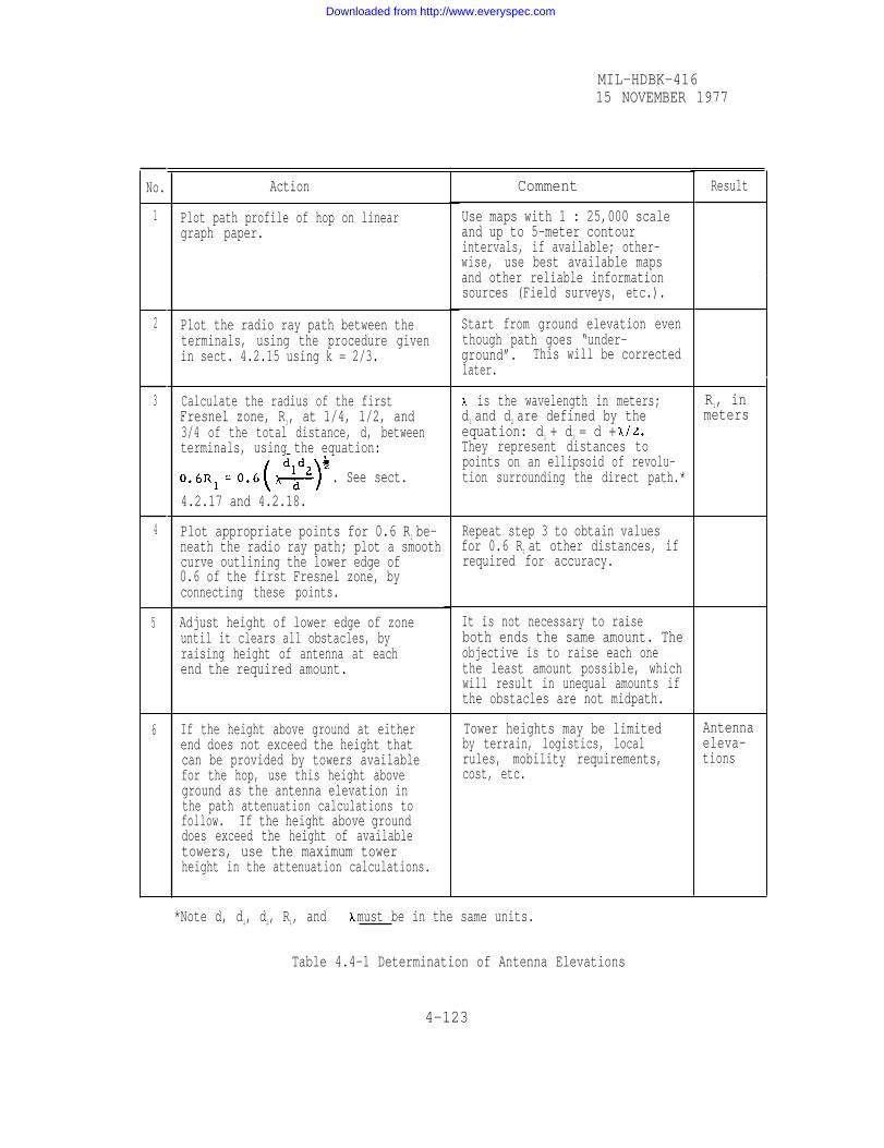
No.
5
6
Action
Plot path profile of hop on lineargraph paper.
Plot the radio ray path between theterminals, using the procedure givenin sect. 4.2.15 using k = 2/3.
Calculate the radius of the firstFresnel zone, R1, at 1/4, 1/2, and3/4 of the total distance, d, betweenterminals, using the equation:
. See sect.
4.2.17 and 4.2.18.
Plot appropriate points for 0.6 R1 be-neath the radio ray path; plot a smoothcurve outlining the lower edge of0.6 of the first Fresnel zone, byconnecting these points.
Adjust height of lower edge of zoneuntil it clears all obstacles, byraising height of antenna at eachend the required amount.
If the height above ground at eitherend does not exceed the height thatcan be provided by towers availablefor the hop, use this height aboveground as the antenna elevation inthe path attenuation calculations tofollow. If the height above grounddoes exceed the height of availabletowers, use the maximum towerheight in the attenuation calculations.
Comment
Use maps with 1 : 25,000 scaleand up to 5-meter contourintervals, if available; other-wise, use best available mapsand other reliable informationsources (Field surveys, etc.).
Start from ground elevation eventhough path goes “under-ground”. This will be correctedlater.
is the wavelength in meters;d1 and d2 are defined by theequation: dl + d2 = d +They represent distances topoints on an ellipsoid of revolu-tion surrounding the direct path.*
Repeat step 3 to obtain valuesfor 0.6 R1 at other distances, ifrequired for accuracy.
It is not necessary to raiseboth ends the same amount. Theobjective is to raise each onethe least amount possible, whichwill result in unequal amounts ifthe obstacles are not midpath.
Tower heights may be limitedby terrain, logistics, localrules, mobility requirements,cost, etc.
*Note d, dl, d2, R1, and must be in the same units.
Table 4.4-1 Determination of Antenna Elevations
4-123
Result
MIL-HDBK-41615 NOVEMBER 1977
1
2
3
4
Antennaeleva-tions
R1, inmeters
Downloaded from http://www.everyspec.com

Figure 4.4-2
MIL-HDBK-41615 NOVEMBER 1977
4-124
Downloaded from http://www.everyspec.com

MIL-HDBK-41615 NOVEMBER 1977
be seen from figure 4.4-2, an 85 m tower height is required for a 50 km
path while only a 56 m height is required for a 40 km path.
4.4.5 Line-of-sight propagation over smooth earth and irregular
terrain
4.4.5.1 For a linear, isotropic, homogeneous medium, propagation
is in a straight line; the amplitude is subject to the inverse distance
law, and the phase varies linearly with distance. This “free-space”
propagation is a convenient reference for the design of line-of-sight
radio links since the median atmosphere and the terrain usually can be
approximated as a piece-wise homogeneous medium by application of
the effective-earth-radius concept. In this sense, with proper system
design (site selection, etc.), the reference condition is commonly
achieved for median atmospheric conditions, and the observed signal
variations are not serious during most of the time. Serious variations
such as deep fading generally occur in certain geographical locations
and at particular times of the day and year; i. e., under certain meteor-
ological conditions (marked departures from the median refractivity
structure) and terrain geometries. Such conditions are sufficiently
understood in most cases to be categorized in terms of why, where,
and when, but their predictability is not suitable for inclusion in formal,
probabilistic, telecommunication-system-design procedures. However,
these conditions can be described so that the systems engineer, in the
course of his site survey, could recognize those paths for which fading
is likely to occur. As design constraints permit, he can then either
avoid the cause of fading or incorporate appropriate remedies.
4.4.5.2 The most basic definitions of fading are in terms of the
propagation mechanisms involved: refraction, reflection, diffraction,
scattering, focusing, absorption, etc., as well as the guiding of radio
waves. These are basic because they determine the statistical
4-125
Downloaded from http://www.everyspec.com
MIL-HDBK-41615 NOVEMBER 1977
behavior with time of the measurable field parameters (amplitude,
phase, and polarization) and the frequency or spatial selectivity of the
fading. The purpose here is to describe the manner in which atmos -
phere and terrain support these mechanisms in terms of simple ray
theory referencing the appropriate sources for further detailed quanti-
tative evaluation. Although simple ray theory is ideal for visualizing
atmospheric and terrain effects, a full description requires wave
theory, asymptotic propagation theory or extensions of ray theory.
4.4.5.3. It has already been shown in Section 4.2.21 that the transmis-
sion loss is free space for line-of-sight links can be expressed as
(4.4-1)
where all terms are in dB. Lbf is the free-space basic transmission loss
from (4.2-20), and Gt and Gr are the expected antenna power gain (relative
to an isotropic radiator) for the systems design conditions. An additional
attenuation A, attributable to atmospheric and terrain effects, must be con
sidered in system design, particularly in fading situations, when it becomes
excessive. For long-term value, a term Aa dB is added to L which repre-
sents the average atmospheric absorption as discusses in Section 4.2.22.
4. 4.6 Refractive index gradients
4.4. 6.1 This section briefly describes some of the available informa-
tion about the refractive index structure near the earth’s surface that
is significant in connection with microwave fading mechanisms. Much
of the material in sections 4. 4.6 through 4.4.20 was taken from [35].
4.4. 6.2 The average bending of an electromagnetic wave propagated
through the troposphere may usually be represented by ray theory in
terms of a radius of ray curvature related to the average gradient of
refractive index. If we assume that the refractive index n of the air
4-126
Downloaded from http://www.everyspec.com

varies linearly with the height h for the first few tenths of kilometer
above the earth’s surface and does not vary in a horizontal direction,
then the radius of curvature r of the radio ray relative to the radius of
the earth, r0 6370 km, may be expressed in terms of the gradient,
by:
(4.4-2)
The parameter k is usually called the effective earth-radius factor.
The gradient is usually expressed in terms of the refractivity,
N=(n- 1) 106, so that
and
(4.4-3)
(4.4-4)
where h is in km. Several values of k and AN/Ah are listed in figure
4.4-3, where the corresponding ray paths are illustrated. The vertical
scale of figure 4.4-3 is exaggerated, relative to the horizontal scale,
to make the differences in curvature noticeable.
4.4.6.3 For 0 < k < 1.0, encountered for positive gradients (subre-
fractive conditions), the ray joining two terminals passes close to the
earth. The ray may even be interrupted by the surface (k = 0.33 in
fig. 4.4-3) so that the receiving terminal is beyond radio line of sight. For
the commonly encountered situations
the rays are farther removed from the earth’s surface. At the critical
and the curvature of the ray
path is equal to the curvature of the earth; thus the ray paths are paral-
lel to the earth’s surface. Conditions for are termed
super critical; the corresponding values of k from (4.4-4) are negative,
and trapping of the radio rays is possible. Consequently, values of
-157 are commonly referred to as a trapping or ducting
4-127
MIL-HDBK-41615 NOVEMBER 1977
value
Downloaded from http://www.everyspec.com
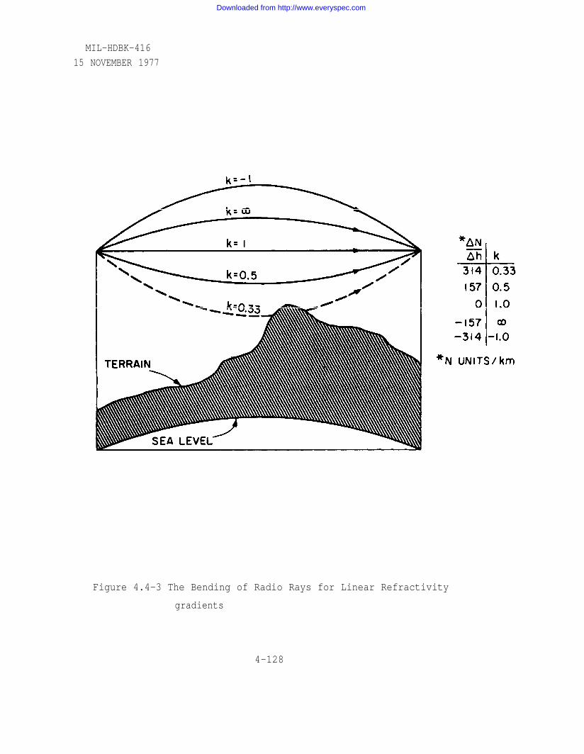
Figure 4.4-3 The Bending of Radio Rays for Linear Refractivity
gradients
4-128
MIL-HDBK-416
15 NOVEMBER 1977
Downloaded from http://www.everyspec.com

gradients. The relation between k and discussed above and dis-
cussed above and given by (4.4-4) is plotted in figure 4.4-4.
4.4.6.4 To illustrate that the range of conditions shown in figure
4.4-4 is realistic, a distribution of average gradients for Cape Kennedy,
Florida, is presented in figure 4.4-5. The distribution was determined
from February, May, August, and November data selected from a 7-
year period. Preliminary y investigations for other locations throughout
the world indicate that figure 4.4-5 at least exemplifies maritime or
coastal locations with relatively smooth terrain. Much of the available
information is included in a recent World Atlas of refractive index
gradients [39].
4.4.6.5 Note that the median
4.4-5 is approximately -60 N
refractive index gradient from figure
units/ km which differs from the com-
monly used median value of approximately -40 N units/km corresponding
to k = 4/3. Even more important is the range of gradients which must be
considered when plotting terrain profiles. A profile plotted for k = 4/3 or
a value corresponding to the median gradient can be very misleading -- it
corresponds to a situation that is not particularly significant for fading
situations and can obscure the dynamic nature of microwave propagation
through the lower atmosphere. Preferable procedures are available. For
example, charts are commercially available for plotting the various ray
paths between two terminals (such as in fig. 4.4-3) for a range of k values.
This is applicable to any profile but avoids much computation when the
profile is a simple rectangular height-versus-distance profile taken
directly from a map.
4.4.6.6 Strong refractive index gradients
occur over a limited range of elevation (layers) at, or above, the ter-
rain surface.
4.4.6.7 Figure 4.4-6 illustrates those super refractive surface gradi-
ients caused by the radiation of heat from the surface to a clear sky.
4-129
MIL-HDBK-41615 NOVEMBER 1977
Downloaded from http://www.everyspec.com

Figure 4.4-4 Effective Earth Radius Factor versus theLinear Refractive Gradient
4-130
MIL-HDBK-41615 NOVEMBER 1977
Downloaded from http://www.everyspec.com
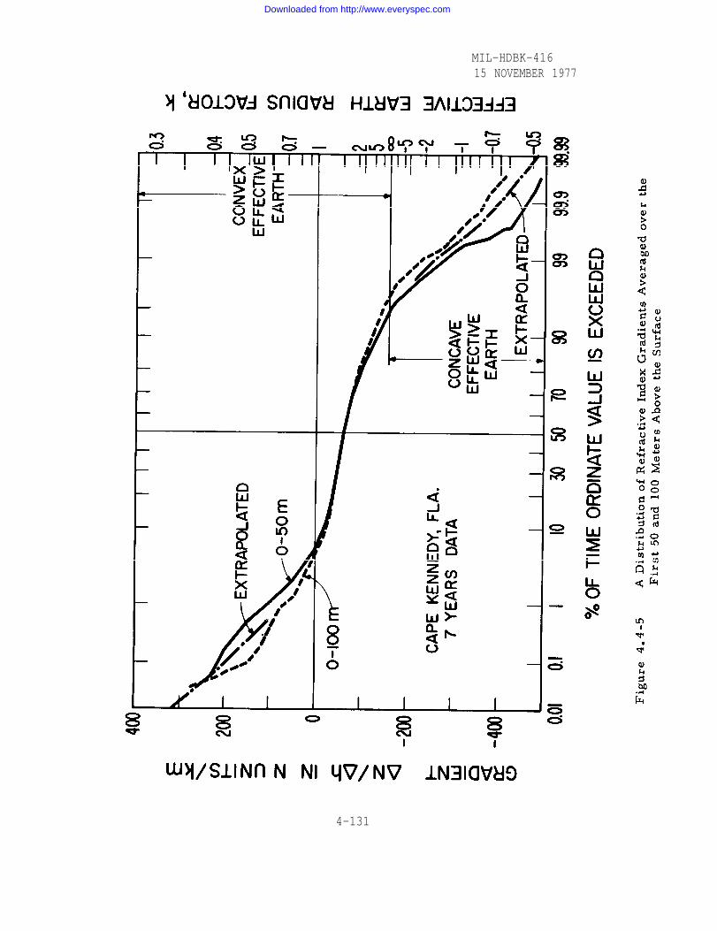
Figure 4.4-5
15 NOVEMBER 1977
4-131
MIL-HDBK-416
Downloaded from http://www.everyspec.com

Figure 4.4-6 4-132
MIL-HDBK-41615 NOVEMBER 1977
Downloaded from http://www.everyspec.com

At night, clear skies and light surface winds permit
MIL-HDBK-41615 NOVEMBER 1977
considerable cool-
ing of the earth’s surface. This can cause the formation of a tempera-
ture inversion (an increase of temperature with height) and produce a
strong super refractive gradient near the surface -- a condition that
can cause substantial fading on microwave links.
4.4.6.8 Extreme subrefractive or superrefractive gradients are less
likely to occur above rough terrain. Line-of-sight propagation paths
between high points of mountainous terrain will, in general, have more
linear distributions of gradients with reduced standard deviations
(compared to that depicted in figure 4.4-5). Thus the amount of fading
and variations in signal level may be greatly reduced. There are
exceptions to this, such as in the coastal range of mountains of northern
Chile, where larger gradients are attributable to the intrusion of the
trade wind inversion among the mountain peaks. Also the median
refractive index gradients for oversea paths are less (more
A detailed, informative treatment of the refraction of radio
the refractive index structure of the lower atmosphere may
negative),
waves and
be found in
[38].
4.4.7 Determination of the range of refractivity gradients
4.4.7.1 If adequate information on the space and time variations of
refractivity gradients were always available, rather exact microwave
design procedures could be developed. At the present time, however,
knowledge of refractivity variations is somewhat limited. The avail-
able statistical data are based largely upon studies of radiosonde obser-
vations (RAOBs) taken routinely by weather services in most parts of
the world. These observations are generally made no more than twice
each day, and at widely separated points (distances of 250 to 400 km
between stations are common in the U.S.), and they do not provide
sufficient detail on thin atmospheric layers which can have a significant
effect on radio propagation. Nevertheless, statistics accumulated from
4-133
Downloaded from http://www.everyspec.com
MIL-HDBK-41615 NOVEMBER 1977
the RAOB data can be used to advantage in the design of line-of-sight
links, particularly when there is no record Of operational experience
in an area in which a new microwave system is being considered.
4.4.7.2 Statistics of refractivity obtained from climatological RAOB
data have been used to prepare the “World Atlas of Atmospheric Radio
Refractivity” [39].This presents a variety of information in the form
of maps, graphs, and tables, including the following:
a.
b.
c.
d.
World maps of monthly mean (the difference in
refractivity between the surface and 1 km),
Mean surface refractivity (NS) for each month for more
than 250 stations in all parts of the world.
World maps of the surface-based 100 m layer gradient
probability, (based upon an analysis of about 100
stations), 4 months of the year.
Cumulative probability distribution graphs of surface-
based 100 m gradients for 22 stations 4 months of the
year.
Thus this atlas provides a convenient source of information upon which
to base estimates of extreme refractivity gradients (super refractive
and subrefractive) in all parts of the world. However, it does not pro-
vide as much detail as is desirable for link design, except for a rela-
tively few locations,and should therefore be supplemented with other
data whenever possible.Additional refractivity data for certain areas
may be available from the Air Force Environmental Technical Applica-
tions Center, Washington,D.C. or from communications laboratories
in various countries.
4.4.7.3 It may sometimes be desirable to obtain RAOB data from a
nearby station and calculate the observed refractivity gradients (for
example, during a period of path testing). The following equation is
used [73]:
4-134
Downloaded from http://www.everyspec.com

MIL-HDBK-41615 NOVEMBER 1977
where
(4.4-5)
N = refractivity in N units
P = pressure in millibars
T = temperature in degrees Kelvin
e = saturation vapor pressure in millibars *s
RH = relative humidity in percent.
Since the gradients are usually given in terms of “N units/ km”; the
height interval of the observation must be noted. Thus, if the refrac-
tivity at the surface is 350 N units and at 100 m the value is 330, the
gradient over the 100 m interval is -200 N units/km. A very conven-
ient nomogram [64] is available for determining refractivity directly
from parameters used in RAOB reports (pressure, temperature, dew-
point), and is reproduced here in figure 4.4-7. When carefully used,
this provides sufficient accuracy for most engineering investigations.
4.4.7.4 A graphical means of obtaining the effective earth’s radius
factor k from refractivity gradient data was shown in figure 4.4-4.
4.4.7.5 The limitations of RAOB-derived refractivity estimates
should be kept in mind when applying these data to design problems. A
RAOB station near the coast is likely to experience very different low-
level gradients than a location even a few miles inland. Differences in
elevation : terrain roughness, vegetation, and exposure to prevailing
winds may result in
also are indications
the point radiosonde
significant local variations in gradients. There
that the extreme gradients sometimes indicated by
observations reflect conditions that exist over a
* See Smithsonian Meteorological Tables.
4-135
Downloaded from http://www.everyspec.com

Figure 4.4-7 Refractive Index Nomogram.
4-136
MIL-HDBK-41615 NOVEMBER 1977
Downloaded from http://www.everyspec.com

very small area, and that the average conditions over an entire radio
path in the same vicinity would be considerably less severe.
4.4.8 Fading mechanisms
4.4.8.1 The significance of the refractive index structure for micro-
wave fading is best illustrated by the variety of situations that produce
such fading. Here we classify and illustrate these fading mechanisms
and identify the supporting refractive index STRUCTURES. A general
discussion of the fading signal characteristics and their remedies is
provided.
4.4.8.2 Fading at microwave frequencies for line-of-sight paths
through the troposphere may be categorized as multipath fading and
power fading. Each category includes several fading mechanisms with
characteristics that often permit their identification.
4.4.9 Multipath fading
4.4.9.1 As the refractive index gradient varies, multipath fading
results from interference between the direct wave and
a. the specular component of the ground-reflected wave;
b. nonsecular components of the ground-reflected wave;
c. partial reflections from atmospheric sheets or elevated
layers; or
d. additional direct (nonreflected) wave paths.
These additional direct wave paths in (d.) can occur due to either the
surface layers of strong positive refractive index gradients or the hori-
zontally distributed changes in refractive index -- as may be encounter-
ed with a weather front. These multipath fading mechanisms are
illustrated in figure 4.4-8.
4.4.9.2 The depths of fades encountered for these multipath phenom-
ena can be quite severe, depending upon the effective reflection
4-137
MIL-HDBK-41615 NOVEMBER 1977
Downloaded from http://www.everyspec.com

Figure 4.4-8
MIL-HDBK-41615 NOVEMBER 1977
4-138
Downloaded from http://www.everyspec.com

MIL-HDBK-41615 NOVEMBER 1977
coefficients or the relative amplitudes of the component waves. Mecha-
nisms (a) and(c) can produce fades persisting for minutes. During such
fades the nonsecular-ground-reflected components (normally small for
small grazing angles) can cause additional interference (with the direct
plus specular component), providing even deeper, more rapid fades
having durations of the order of seconds. An illustration of multipath
fading (direct plus ground-reflected wave) is presented in figure 4.4-9
to show the characteristic return of signal level to, or above, the free-
space value. In figure 4.4-9, a basic transmission loss [8] of approxi-
mately 139 dB corresponds to that for the free-space signal level.
Multipath fading tends to be less frequent during the day, particularly
during the afternoon hours, when conditions more closely approach a
median or reference atmospheric structure with constant gradients.
4.4.9.3 Figure 4.4-10 is an illustration of the frequency selectivity
of multipath fading and shows recordings of received signals of two
transmission frequencies over a common propagation path. On an
instantaneous basis the two recordings appear uncorrelated. Note,
however, that with an allowance for time lag the two signals appear to
be highly correlated. This time lag for high correlation, which is a
measure of the effective (frequency) diversity separations is a function
not only of the frequency separation, but also of the refractive index
gradient and its time rate of change. Thus the frequency spacing of
figure 4.4-10 is inadequate if fades of 20 dB below the 139 dB free-
space level are unacceptable.
4.4.9.4 The multipath fading due to the interference from specular
ground reflections can be avoided by eliminating one of the field com-
ponents. The specularly reflected wave can be severely reduced by
special “anti-reflective wave” antenna arrays [37], [58] or by the use
of Fresnel zone screens [46], [69], and [74]. These devices assume
4-139
Downloaded from http://www.everyspec.com

Figure 4.4-9
MIL-HDBK-41615 NOVEMBER 1977
4-140
Downloaded from http://www.everyspec.com

MIL-HDBK-41615 NOVEMBER 1977
Figure 4.4-10 Example of Frequency Selectivity for MultipathFading
4-141
Downloaded from http://www.everyspec.com
MIL-HDBK-41615 NOVEMBER 1977
that the range of refractive index gradients will not be too great. For
propagation over rough irregular terrain, this last condition is usually
met, and the effects of ground reflections may then be avoided by the
proper choice of antenna sites or antenna designs. To date, however,
the most effective counter measure for general multipath fading over
wide ranges of refractive index gradients is diversity reception [36],
[47], [59], and [60].
4.4.10 Multipath characteristics
4.4.10.1 Multipath fading caused by reflection from the sea or land
surfaces or from layering in the atmosphere produces amplitude varia-
tions of the received signal level characterized by: (1) the maximum
signal between fades exceeding, to some extent, the free-space level,
(2) frequency and duration of fades related not only to the path geometry
and transmission frequency but also to the variation of the refractive
index structure with time, and (3) usually one of a specific family of
signal level distributions. A quantitative description of these character-
istics will provide a means of identifying the probable causes of fading
when it is observed.
4.4.10.2 The peak values of multipath signal levels depend upon the
number of signal components and their relative amplitudes and simply
correspond to the sum of all component voltages. Similarly, the num-
her, relative amplitude, and relative phases of the components deter-
mine the cumulative distribution of the levels corresponding to their
vector sum. The first requirement, therefore, is a description of the
relative amplitudes and phases of the component voltages. This is not
practical, at present, for all the situations of interest. Although
there have been significant advances in the theoretical treatment of
reflection or scattering from atmospheric layers in terms of specific
refractive index profiles [43], [52], and [76], and experimental
4-142
Downloaded from http://www.everyspec.com

MIL-HDBK-41615 NOVEMBER 1977
investigations have been reported, the state-of-the-art has not yet pro-
vided engineering expressions for the magnitude and phase of the multi-
path components that produce severe fades at microwave frequencies
and are attributable to reflection from atmospheric layers. We can,
however, identify the distributions of signal amplitudes that would be
expected; they coincide with those encountered for multipath produced
by reflection and scattering from irregular terrain, and signal character-
istics will be quite similar to those shown in figures 4.4-9 and 4.4-10.
4.4.11 Power fading
4.4.11.1 Power fading results from the partial isolation of the trans-
mitting and receiving antennas because of:
a. intrusion of the earth’s surface or atmospheric layers
into the propagation path (earth-bulge fading or diffraction
fading*);
b. antenna decoupling due to variation of the refractive
index gradient;
c. partial reflection from elevated layers interpositioned
between the terminal antenna elevations;
d. "ducting" formations containing only one of the terminal
antennas; and
e. precipitation along the propagation path.
*When a strong atmospheric layer intrudes into the direct propagationpath between transmitter and receiver, the effect is much like thatfor intrusion of the earth’s surface. For example, the energy repre-sented by ray paths which strike the surface of a super refractivelayer, at grazing angles of more than a few milliradians, penetratesthe layer and is diverted from the direct path to the receiver location.The ray path at grazing incidence and those ray paths which passabove the layer provide a contribution to the receiver in the radio holeor "shadow” of the layer via the diffracted mode of propagation.
4-143
Downloaded from http://www.everyspec.com

MIL-HDBK-41615 NOVEMBER 1977
The received signal for these power fading mechanisms is characterized
by a marked decrease in median signal level below that for free space
and for extended periods of time. Some examples of these fading
mechanisms are given in figure 4.4-11.
4.4.11.2 Power fading due to subrefractive index gradients is not
likely to happen if adequate terrain clearance is provided, and does not
commonly occur on well designed line-of-sight paths. Due to their low
probability of occurrence and difficulty of analysis, quantitative predic-
tion methods for such types of fading have not been developed, although
their effect is significant because there is no diversity improvement
and they often last much longer than multipath fades when they occur.
4.4.12 Power fading due to diffraction
4.4.12.1 The power fades that occur due to diffraction by the earth’s
surface are generally caused by a subrefractive (positive) gradient of
refractive index as illustrated by the upper diagram of figure 4.4-11.
This type of fading can persist for several hours and to depths of 20 or
30 dB below the free-space level. Such fading is essentially independent
of small-scale changes in frequency, but may be reduced or avoided by
proper choice of terminal antenna heights.
4.4.12.2 In mountainous terrain where terminals are located on
dominating ridges or peaks, a clearance corresponding to a single
Fresnel zone or less will usually be sufficient. The required clearance
at mid path corresponding to n Fresnel zones in meters is
(4.4-6)
from (4.2-17) subject to the same limitations as stated in paraqraph
4.2.18.4. Here the path length d is in kilometers and the transmission
frequency f is gigahertz. If only a limited range of refractive
Index gradients is encountered, a
or less is sufficient. For those
first Fresnel zone clearance, C1,
microwave paths where subrefractive
4-144
Downloaded from http://www.everyspec.com

Figure 4.4-11
MIL-HDBK-41615 NOVEMBER 1977
4-145
Downloaded from http://www.everyspec.com

MIL-HDBK-41615 NOVEMBER 1977
index gradients are encountered, increased clearances are required.
Consider a 2 GHz, 50 km propagation path with terminal antennas at
equal heights. The smooth spherical earth diffraction loss for such a
path is shown in figure 4.4-12 as a function of antenna height and path
length when the refractive index gradient is 80 N units/km (correspond-
ing to k 2/3). Generally, the path length d in kilometers, the effec-
tive earth radius factor k (related to the gradient through 4.4-4,
and the antenna heights, h1, and h2 in meters, for which the path would
be just grazing (i.e., barely line-of-sight) are related by
(4.4-7)
This expression involves the familiar relation between antenna height
and horizon distance over smooth earth, modified here for the metric
system of units. For h1 = h2 = 36.73 m and k = 4/3, such a path
would be just barely line-of-sight. A first Fresnel zone clearance,
C1 = 43.3 m from 4.4-6, would therefore require terminal antenna
heights of approximately 80 m. Such a path would, however, still
experience an attenuation of 10 dB for = 80 N units/km (see
figure 4.4-12) and 23 dB for = 160 N units/km. TO protect
against a particular depth of diffraction fading, we must specify the
required clearance in terms of the subrefractive gradients that may be
encountered and the shape of the obstructing terrain.
4.4.12.3 Diffraction fading in the sense used earlier may also occur
when a strong super refractive layer is positioned slightly below the
terminal antennas. This was described in the footnote of paragraph
4.4.11.1 and is illustrated in figure 4.4-13. In such a situation the
grazing condition is given by (4.4-7) when the hl and h2 are the heights
of the antennas above the top of the layer and k corresponds to the
average gradient between each antenna and the top of the layer. This
4-146
Downloaded from http://www.everyspec.com

MIL-HDBK-41615 NOVEMBER 1977
Figure 4.4-12 Attenuation Curves for a 2 GHz PropagationPath
4-147
Downloaded from http://www.everyspec.com

Figure 4.4-13
MIL-HDBK-41615 NOVEMBER 1977
4-148
Downloaded from http://www.everyspec.com

MIL-HDBK-41615 NOVEMBER 1977
situation is known as a radio hole in air-to-air applications [48], and [50].
The fading loss can be severe and may be estimated at grazing from calcu-
lating the parameters listed in figure 4.4-14, and using the curve given
therein [49]. The severity of this type of fading will be reduced somewhat
by terrain reflections or contributions from subrefractive layers posi-
tioned below the diffracting layer, which can direct energy back toward the
receiver. These contributions, illustrated in figure 4.4-13, are a function
of the gradients within and below the diffracting layer and also of the ter-
rain roughness. They may, however, also produce multipath fading.
4.4.13 Power fading due to antenna “decoupling”
4.4.13.1 Power fading due to antenna “decoupling” refers to the loss of
signal that occurs for transmission and reception of the signal outside
of, or at the extremities of, the main lobe of the antenna pattern. For
example, variations were observed in the vertical angle-of-arrival of
up to 0.5° on a 38.6 km line-of-sight path [72]. This effect is propor-
tional to the path length and can introduce several decibels of loss for
high gain antennas and long line-of-sight paths. Such losses may be
minimized by specifying a sufficiently broad antenna beam so that the
expected variations of the angle-of-arrival are matched or exceeded.
The variation is most conveniently expressed relative to the angle-of-
arrival for flat earth (k = ) conditions. Thus, at the terminal
antenna elevation is h1 m, the angle-of-arrival from an antenna
elevation of h2 m and d0 km distant, is given (for k = ) by*
or, for most practical situations where is small,
whose
at an
(4.4-8)
(4.4-9)
* hl and h2 are measured relative to a common reference elevation suchas mean sea level.
4-149
Downloaded from http://www.everyspec.com

Figure 4.4-14 Attenuation of a Field Due to Diffractionby a Smooth Spherical Earth at ExactlyGrazing Conditions and Relative to theFree Space Field
4-150
MIL-HDBK-41615 NOVEMBER 1977
Downloaded from http://www.everyspec.com

MIL-HDBK-41615 NOVEMBER 1977
(4.4-10)
or
For situations that may be approximated by a linear gradient, k is
given by (4.4-4) and the angle-of-arrival will be
(4.4-11)
For high gain antennas, super refractive conditions (negative k-values)
will tend to enhance the reception of ground reflected rays, and subre-
fractive conditions (positive k-values less than unity) will tend to en-
hance the contributions from elevated layers, etc. This should be
clear from (4.4-10), since k is positive and greater than unity for
common design practice. Negative k-values then cause the angle-of-
arrival to exceed that for which the antennas are oriented. Similarly,
for 0 < k < 1.0, the angle-of-arrival is less than that for the design
conditions.
4.4.14 Power fading due to ducts and layers
4.4.14.1 Power fading due to atmospheric ducts and elevated layers,
(c.) and (d.) in 4.4.11.1 is characterized by fades of 20 dB and occasion-
ally greater values. They may persist for hours or days, but tend to
be less frequent during daylight hours. This type of mechanism is the
likely source of many phenomena which have been termed space-wave
fadeouts. The fading is not generally sensitive to small-scale (in-band)
changes of frequency or of spatial position of the antennas, and cannot
therefore readily be remedied by commonly used diversity techniques.
4.4.14.2 An elevated duct is sometimes a combination of elevated
layers, such as the occurrence of a super refractive layer above a
subrefractive layer, and has the effect of guiding or focusing the signal
energy along it. The reverse can also occur; the combination of a
refractive layer above a super refractive layer will defocus energy
4-151
sub-
Downloaded from http://www.everyspec.com

MIL-HDBK-41615 NOVEMBER 1977
introduced within the combination of layers.For terminals within such
a combination,the defocusing effect will produce a power fade.
4.4.14.3 Obviously, repositioning of one or both antennas can elimin-
ate the problem --see the two lower diagrams of figure 4.4-11 -- and
in some situations this is feasible, although major height changes may
be required.For effective repositioning of the antennas, some informa-
tion about layer characteristics (prevalence, thickness, height, etc.)
is required.For example, the likelihood of isolation for long paths is
reduced by locating both terminal antennas at the same height relative
to the expected duct or layer position. For short paths, however, the
likelihood of isolation can be reduced by a sufficiently great difference
in antenna heights to insure that the angle of ray-path incidence at the
elevated layer is at least on the order of a few degrees.
4.4.15 Fadingdue to precipitation
4.4.15.1 Power fading can also occur due to signal attenuation by
extensive precipitation along a propagation path [20]. The effects of
this fading can be lessened by route diversity which is the use of an
alternate series of communication links [54], [63], and has been
discussed
4.4.16
4.4.16.1
in section 4.2.6.
Combinations of fading mechanisms
For many propagation paths, more than one fading mechanism
will be involved,
tive index. TWo
some are k-type
their relative significance changing with the refrac-
particular combinations that can be especially trouble-
fading as described below, and surface-duct fading.
4.4.17 k-type fading
4.4.17.1 The k-type fading occurs for propagation over smooth or uni-
formly irregular terrain such as the sea surface, maritime terrain or
gently rolling (pastoral) terrain. The mechanism involves either the
multipath fading (direct ray plus ground reflections) or the diffraction
4-152
Downloaded from http://www.everyspec.com

MIL-HDBK-41615 NOVEMBER 1977
type of power fading, depending upon the value of the earth-radius
factor k [62]. The two mechanisms supplement one another and produce
fading throughout a wide range of refractive index gradients or k-
values. Resulting signal variations are illustrated in figure 4.4-15
which is a graph of the envelope of spherical-earth transmission loss
versus refractive index gradient. It also shows the effect of terrain
roughness (expressed here by the ratio and takes into account the
divergence-convergence factor under the dynamic influence of the re-
fractive index gradient. The ratio is that of the standard deviation,
of the surface irregularities (about a median spherical surface) to
the transmission wavelength, (both expressed in the same units).
For a smooth earth the fading produced by the interference
between the direct wave and the specularly reflected wave is serious
only over a limited range of refractive index gradients. For the path
parameters of figure 4.4-15 as an example, the fades due to the inter-
ference nulls can exceed 20 dB only within the range of -115 to -195
N units/km and for gradients in excess of 300 N units/km. As the
surface roughness is increased the critical region Of gradients
for 20 dB fades shifts to more negative values and becomes wider --
for The graph shows a range of -180 to -290 N units/km.
Irregularities or roughness that would cause the median terrain surface
to depart slightly from a sphere could also shift the range of critical
negative gradients in either direction. Naturally, these critical ranges,
as well as the region of diffraction fading depend upon the specific link
parameters (transmission frequency, antenna height, and path length) .
One aspect should be clear from figure 4.4-15: unless the terrain
roughness is sufficient to shift the critical range of negative gradients
outside of the range of refractive index gradients expected to occur at a
particular location (see figure 4.4-5 for example), reflections from the
terrain surface cannot be considered to eliminate terrain reflection
4-153
Downloaded from http://www.everyspec.com
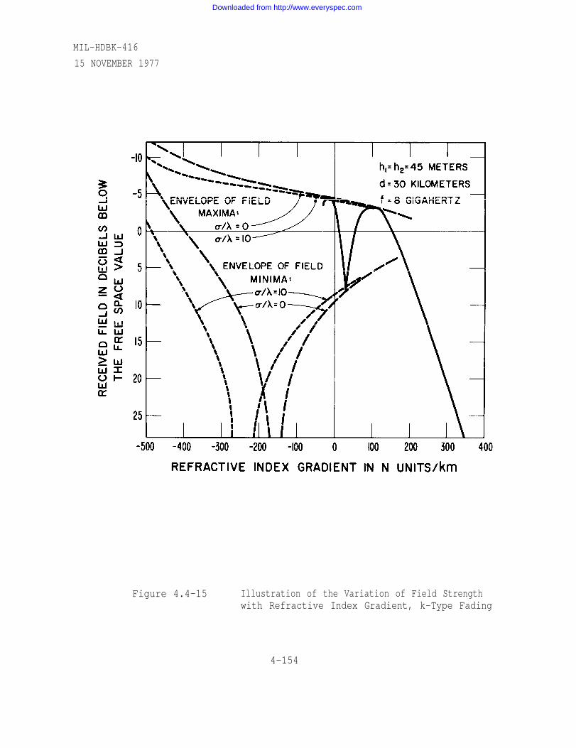
MIL-HDBK-416
15 NOVEMBER 1977
Figure 4.4-15 Illustration of the Variation of Field Strengthwith Refractive Index Gradient, k-Type Fading
4-154
Downloaded from http://www.everyspec.com

MIL-HDBK-41615 NOVEMBER 1977
unless they also partially obstruct the reflected wave over the critical
range of refractive index gradients.
4.4.17.2 The effects of k-type fading are reduced by (1) increasing the
terminal antenna heights to provide adequate protection against the dif-
fraction fading for the expected extreme positive gradients of refractive
index; and also (2) diversity reception that effectively reduces the atten-
uation due to multipath out to the expected extreme negative gradients of
refractive index. An applicable design procedure was first proposed
and demonstrated as reported in [59]. A more accurate extension of
such design procedures is given in [49] and [67] .
4.4.18 Surface duct fading
4.4.18.1 Surface duct fading is encountered on long, line-of-sight,
over-water paths. Sea surface ducts may constitute a semipermanent
condition as, for example, in the region of the Bermuda High, a high-
-pressure region of the Atlantic between 10° and 30° N latitude. There,
the ducts form less than 2 km from the shore and extend from the sea
surface up to heights of 7 to 20 m for wind velocities from 15 to 55 km/hr.
They persist during fair weather and reform after squalls and rain
showers [57]. The corresponding fading mechanism is a combination of
multipath fading (for reflections from the sea) and power fading in the
presence of the sea surface duct. These two mechanisms are illustrated
in figure 4.4-16. Because of the continual disturbance of the sea sur-
face, a reflected wave consists of a diffuse or randomly distributed
component superimposed upon the specular component, and its time dis-
tribution is a Beckmann distribution consisting of a constant component
plus a Hoyt distribution [40], and [55]. This constitutes the received
field for the upper diagram of figure 4.4-16. Addition of the direct
wave, as in the situation illustrated by the lower diagram of figure
4.4-16, produces an enhanced or reduced constant component due to
4-155
Downloaded from http://www.everyspec.com

Figure 4.4-16
MIL-HDBK-41615 NOVEMBER 1977
4-156
Downloaded from http://www.everyspec.com

MIL-HDBK-41615 NOVEMBER 1977
phase interference. One effect of the surface duct upon the multipath
situation is to provide an increased angle of incidence for the energy
reflected from the sea surface. This reduces the reflection coefficient
and thereby increases the ratio of the diffused to specular amplitudes,
and increases the rapidly varying component of the reflected signal.
The net result is a total signal whose distribution approaches the
Nakagami-Rice distribution, a constant plus a Rayleigh-distributed
variable [44], [65], [66], [67], and [71].
4.4.18.2 Surface or ground-based ducts guide or trap the radio
waves by the combination of a strong negative refractive index gradient
(superrefraction, -157 N units/km) and a reflecting sea or
ground. Propagation within the duct has been described in [53] result-
ing from an equivalent linear gradient of refractive index, and is illus-
trated on the right-hand side of figure 4.4-17. The field may result
from phase interference between a direct wave and one to three singly
reflected waves. For sufficiently strong super refraction, doubly re-
flected waves may contribute.
4.4.18.3 Surface-duct fading can also be reduced by means of a prop-
er adaptation of procedure [59]. Choosing the initial terminal antenna
heights to provide adequate Fresnel zone clearance (above the ducting
layer) avoids the situation shown in the upper drawing in figure 4.4-16.
Similarly, lower antenna heights could achieve the situation shown in
the lower drawing of figure 4.4-16. In the latter case, diversity recep-
tion would also be required because of the multipath effect.
Multipath fading characteristics have already been described
in section 4.4.10. In order to obtain distribution curves for the re-
ceived signal level values one must first evaluate the amplitude and
phase relations of the various multipath components.
4-157
Downloaded from http://www.everyspec.com

Figure 4.4-17
MIL-HDBK-41615 NOVEMBER 1977
4-158
Downloaded from http://www.everyspec.com

MIL-HDBK-41615 NOVEMBER 1977
4.4.19 The relative amplitudes of the multipath components
4.4.19.1 Theoretical and experimental studies of reflection and scat-
tering from terrain have just recently resulted in engineering expres-
sions that permit an estimate of the reflected and scattered components
[41]. For the particular case of small angles of incidence and the micro-
wave frequencies at which specular reflection from terrain results in
significant fading, the Fresnel reflection coefficients modified by a
divergence factor may be taken as essentially unity (with a 180° phase
shift upon reflection). The specular reflection coefficient then becomes
equal to the factor [41]:
(4.4-13)
where
(4.4-14)
Here, is the standard deviation of the irregular terrain about its mean
elevation (as before), is the transmission wave length, and is the
angle of incidence (zero for grazing conditions) must be in the
same units. The expression for m is recognizable as related to the
Rayleigh criterion for roughness (see paragraph 4.2.19.2). The specular-
ly reflected component is therefore given where g is the geometric
mean of the transmitting and receiving antenna power gain values (as
ratios, not in dB) for the reflected ray path relative to those for the
direct path. In addition to this specularly reflected component, there is
the random field scattered by the irregularities of the atmosphere and/or
the reflecting terrain. The rms value of this non-specularly reflected
component depends upon the reflecting surface’s distribution and corre-
lation function, but is almost always appreciably less than
4-159
(4.4-15)
Downloaded from http://www.everyspec.com

MIL-HDBK-41615 NOVEMBER 1977
4.4.20 The received signal amplitude distributions
4.4.20.1 In general, the multipath fading mechanisms produce two or
more components with varying relative phases. Even when several
components are involved, one or two of them tend to be dominant. For
this reason, one would generally not expect a Rayleigh-distributed
received signal. The departure from a Rayleigh distribution will take
one of two forms, depending upon the nature of the field components.
4.4.20.2 For grazing angles of more than a few milliradians, the
specularly reflected wave tends to be small, while the randomly (non-
specularly) reflected components tend to provide a significant contribu-
tion. The signal distribution tends to be less steep than a Rayleigh
distribution; it consists of a constant direct signal plus a random signal
[42], and [66]. The resulting family of cumulative distributions,
adapted from [40] and [41], is illustrated in figures 4.4-18 through
4.4-22 as a function of the parameters B and K. These distributions
give the percent of the time that the total field strength r will exceed its
rms value by an amount given by the vertical decibel scale expressed
by
Z = 20 log10(4.4-16)
4.4.20.3 The ratio of the constant component (the direct field) to the
RMS value of the random field is indicated by B on the distribution
curves. The parameter K is a measure of the anisotropic scattering of
the random components by the terrain. For a very rough reflecting or
scattering surface, the phases of the random components are uniformly
distributed and K2 is unity. For less rough surfaces, such aS the sea
in fair weather or rolling, pastoral terrain, the pattern of roughness
differs with direction and K2 departs from unity. The distribution of
the randomly reflected or scattered components may be represented by
that for the vector sum of two orthogonal random components -- a Hoyt
4-160
Downloaded from http://www.everyspec.com
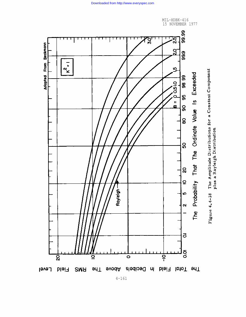
Figure 4.4-18
MIL-HDBK-41615 NOVEMBER 1977
4-161
Downloaded from http://www.everyspec.com
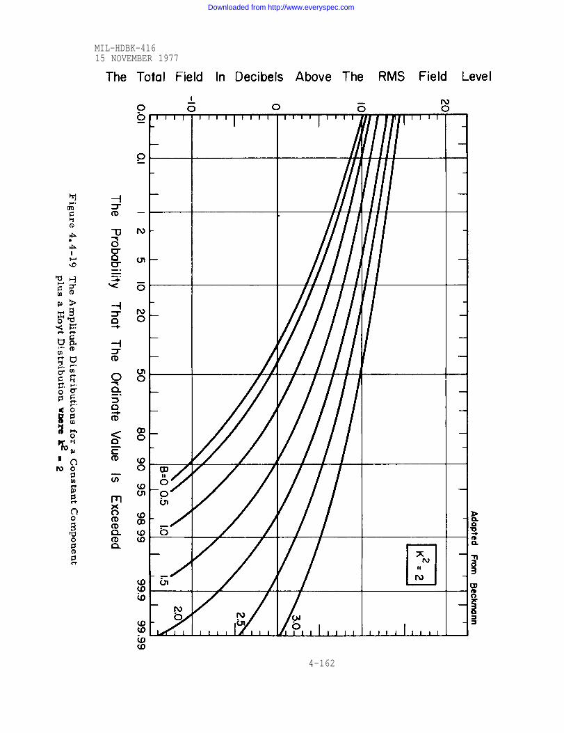
Figure 4.4-19
MIL-HDBK-41615 NOVEMBER 1977
4-162
Downloaded from http://www.everyspec.com

Figure 4.4-20
MIL-HDBK-41615 NOVEMBER 1977
4-163
Downloaded from http://www.everyspec.com

Figure 4.4-21
MIL-HDBK-41615 NOVEMBER 1977
4-164
Downloaded from http://www.everyspec.com

Figure 4.4-22
MIL-HDBK-41615 NOVEMBER 1977
4-165
Downloaded from http://www.everyspec.com
MIL-HDBK-41615 NOVEMBER 1977
distribution. Each component has an amplitude that is normally distri-
buted about a mean of zero and the K2 is the ratio of the variances of
the two distributions.
4.4.20.4 If there is no constant (direct field) component, then B = 0,
and the total field distribution reduces to that for the random components,
a Hoyt distribution [42], and [55]. If, in addition, the surface is ex-
tremely rough so that K2 is unity, the distribution reduces to a Rayleigh
distribution, as in figure 4.4-18 with B = 0. The distributions of figure
4.4-18 for B > 0 are also known as the Nakagami-Rice distribution [44],
[66], [67], and [71].
4.4.20.5 Note that the sum of a direct field and many randomly re-
flected components will produce distributions similar to those given by
figures 4.4-18 through 4.4-22. The distribution, however, actually
implies only that the sum is that of many random components, one of
which is constant and dominant for large values of B; it does not imply
that the components have to be reflections. A variety of alternate pre-
sentations of the information in figure 4.4-18 through 4.4-22 is given
in [40].
4.4.20.6 For very small grazing angles the reflected wave is essen-
tially given by the specularly reflected component. The cumulative sig-
nal distribution caused by interference between the direct wave and this
specularly reflected component tends to be steeper than a Rayleigh
distribution for strong specular reflection. The resultant two-component
multipath distribution are given in figure 4.4-23 for various values of
the reflector coefficient and the rms field for each case is therefore
[50]. The total field is indicated in terms of decibels relative
to this rms value. Similar curves are given in [70]. Again, these
distributions do not necessarily imply a direct wave plus
reflected component from the terrain; they merely imply
a specularly
two constant
4-166
Downloaded from http://www.everyspec.com

Figure 4.4-23
MIL-HDBK-41615 NOVEMBER 1977
4-167
Downloaded from http://www.everyspec.com
MIL-HDBK-41615 NOVEMBER 1977
components with a uniformly distributed difference in phase. Hence
figure 4.4-23, as well as 4.4-18 through 4.4-22, describes conditions
that may be due to any of the multipath fading mechanisms, and addi-
tional information is usually required to distinguish between such
mechanisms.
4.4.20.7 The most general situation, occurring for
angles of incidence, involves two constant components
moderately small
(direct wave plus
the specularly reflected wave) and a randomly distributed component
(caused by nonsecular reflection and atmospheric scattering). A
complete family of such cumulative distribution curves has not been
computed, but an illustrative example is taken from [50] presented in
figure 4.4-24. There , as previously defined, equals unity, and the
rms random field value is indicated by S in decibels above the two-
component rms value, Again, the total field r is express-
ed in decibels relative to the total rms field value
4.4.20.8 In some of the foregoing distributions, an a priori determin-
ation of the signal distribution from the parameter value depends upon
an estimate of the mean power in the random component. In the case of
terrain reflections, an estimate may be obtained from the distribution
and correlation function of the terrain irregularities [41]. However,
these are also often unknown. Frequently, a knowledge of the param-
eters is not necessary; it is usually sufficient to know which family of
distributions is expected. Alternately, one may be interested in com-
paring observed distributions with those of figure 4.4-18 through
4.4-22, so that the likely fading mechanisms may be inferred.
4.4.21 Path fading range estimates
4.4.21.1 Atmospheric considerations. Satisfactory methods of
estimating fading probability on specific paths from climatological
statistics are not available at present. Statistical studies of
4-168
Downloaded from http://www.everyspec.com

Figure 4.4-24
MIL-HDBK-41615 NOVEMBER 1977
4-169
Downloaded from http://www.everyspec.com
MIL-HDBK-41615 NOVEMBER 1977
refractivity can, however, provide information on relative gradient
probabilities for different areas, and indicate the seasonal changes to
be expected [39]. The low-level refractivity gradients that are of most
importance to line-of-sight propagation are very sensitive to variations
in the local surface conditions, and therefore the information obtained
on the site surveys can be useful at this stage of link design. Operating
experience on many microwave links shows that:
a.
b.
c.
d.
e.
f.
Fading is more likely on paths across flat ground than
on paths over rough terrain;
There is less fading on paths across dry ground than
on paths across river valleys, wet or swampy terrain,
or irrigated fields;
Calm weather conditions are favorable to the atmos-
pheric stratifications that may result in deep fading;
these conditions occur more often in broad, protected
river valleys than over open country;
Fading is likely near the center of large, slow-moving
anticyclones (high pressure areas). These are more
likely to occur in summer and fall than in winter and
spring;
Fading occurs more frequently and is more severe in
summer than in winter (in temperate climates);
Paths with takeoff angles more than about 0.5° are less
susceptible to fading, and the effect of refractivity
gradients is negligible for takeoff angles above 1.5°
[45].
The empirical method outlined in section 4.2.27 is recommended for
obtaining path fading probability estimates.
4-170
Downloaded from http://www.everyspec.com

. 4.4.21.2
path over
with a 40
As an example of the use of this method, consider a 50 km
flat terrain in a relatively humid region, operating at 6 GHz
dB fading margin:
Therefore, fading exceeding the margin of 40 dB is
during about 0.009% of the year, or 47 minutes. If
estimated to occur
higher reliability
is required, some change in path parameters will be necessary. Pos-
sible diurnal variations in circuit loading should also be considered,
since on overland paths fading occurs about 5 times more frequently at
night than in the daytime [ 3]. Thus in the example above we might
expect only
hours.
4.4.22
4.4.22.1
about 8 minutes of the fading to occur during the daylight
Diversity on microwave relay links
A reliable microwave system can be made into an extreme-
ly reliable one if proper protective actions are taken. There are many
discussions in the literature about reliability and how to improve it for
example in [4] on page 110 to 117.
4.4. 22.2 Throughout this literature, the key word is redundancy.
For example, outage due to equipment failure can be almost complete-
ly eliminated if redundant equipment is available and if a proper main-
tenance procedure is used. Similarly, to combat outages due to
anomalous propagation, one looks for redundant propagation paths.
4.4. 22.3 The most drastic way in which to supply this latter redun-
dancy is to provide the system with two, or even more, distinct sets of
4-171
MIL-HDBK-41615 NOVEMBER 1977
Downloaded from http://www.everyspec.com
MIL-HDBK-41615 NOVEMBER 1977
relay links which traverse entirely different routes. At the receiving
terminal, there are then available two or more signals which carry the
same information but which have undergone degradation of different
amounts at different times. By "combining” these signals (often by
merely switching to the one that is momentarily the best) one can obtain
a more nearly perfect reproduction of the original information. Be-
cause of the diverse routes involved, this technique is called route
diversity. In a restricted sense (restricted, because no dynamic
switching is involved), this is what long-haul lines of a common carrier
are likely to use. The technique has also been suggested [54] as a
very practical way to combat precipitation fading at millimeter waves.
4.4.22.4 The almost universal practice, however, is to use but a
single route and to attempt to make each link of that route as reliable as
possible. Earth bulge fading, for example, is combatted by carefully
choosing antenna heights large enough so that the
potential obstacles, even under the most adverse
conditions.
4.4.22.5 Space-wave fadeouts and other forms
direct ray clears all
subrefractive
of power fading can be
combatted by specifying a sufficiently large fade margin by which the
normally received signal level exceeds the minimum for satisfactory
performance. Although fade margins as low as 20 dB were sometimes
used in the past, today most links are designed to have fade margins of
35 to 40 dB or more. These high signals, incidentally, are provided
for more reasons than merely to protect against fading. If frequency
modulation is used, and if the system is composed of many links, the
same fade margins are also needed to meet basic system noise objec-
tives (sect. 4.5.16). Fading, when it occurs, will most probably effect
only a single link. Although a 20 dB fade on one link will affect total
4-172
Downloaded from http://www.everyspec.com

MIL-HDBK-41615 NOVEMBER 1977
system noise only slightly, the same drop in signal level on all links
will introduce unacceptable noise levels in the system.
4.4.22.6 These first precautions have the highest priority. If, for
one reason or another, it is impossible to provide high enough antennas
or large enough fade margins, the engineer must either look for an
intermediate relay point or resign himself to the consequently lessened
reliability.
4.4.22.7 For still higher degrees of reliability, specular and non-
secular multipath fading must be considered. Since these are caused
by the destructive interference of two or more waves, an interesting
situation presents itself. A change in the phase relation between these
waves may change the destructive interference to constructive inter-
ference. This, of course, actually happens as the atmosphere changes
with time and causes the received signal level to go above and below a
given reference value. On an instantaneous basis, the required change
in phase can be accomplished in two ways. One way is to change the
carrier frequency, using the fact that the relative phases involved are
linear functions of frequent y. The second way is to remember that a
multipath field implies an interference pattern in space, so that a
small change in position of the receiving antenna will also change the
relative phases.
4.4.22.8 These observations lead to the techniques of frequency
diversity and space diversity. In the first, the same message is trans-
mitted on two different frequencies. At the receiving terminal, both
signals are received, amplified, and then combined (perhaps by switch-
ing to the better) assuming that if one fades out, the other will not.
4.4.22.9 When space diversity is used, there is only a single trans-
mission, but at the receiving terminal this transmission is picked up
by two different antennas. For both theoretical reasons and convenience,
4-173
Downloaded from http://www.everyspec.com
it is best to space these vertically along the antenna tower. Then the
two received signals are amplified and combined, again under the
assumption that if one of them fades out, the other will not. Figure
4.4-25 and 4.4-26 are simplified block diagrams which show how these
two techniques might be implemented.
4.4.22.10 It should be emphasized that neither frequency nor space
diversity will combat power fading because power fading may affect the
entire microwave spectrum and large regions of space. When such
fading appears on one received channel, it is most likely to appear
simultaneously on the other.
4.4.22.11 On the other hand, a large fade margin does help to combat
both power fading and multipath fading. In general, the deeper the fade
the more rare is its occurrence. Thus, the larger the fade margin,
the more rarely will it be exceeded.
4.4.22.12 There are other protective actions that might be taken.
Polarization diversity is often mentioned, but is of little use. It would
presumably entail receiving and combining signals on two orthogonal
polarizations. However, at microwave frequencies the two polariza-
tions are affected by the atmosphere in almost identical ways. If one
of these channels fades out, so will the other. (Orthogonal polariza-
tions are often used in frequency diversity systems, but only as a device
to provide added isolation of the two channel s.) Angle diversity and
mode diversity have been tried with some success. They both resemble
space diversity, but use more compact arrangements for the two re-
ceived channels. (Angle diversity uses two feed points on the same
parabolic dish, while mode diversity depends on the excitation of a
secondary mode in the wave guide leading to or from a large horn
antenna. )
4-174
MIL-HDBK-41615 NOVEMBER 1977
Downloaded from http://www.everyspec.com

Figure 4.4-25
MIL-HDBK-41615 NOVEMBER 1977
4-175
Downloaded from http://www.everyspec.com

Figure 4.4-26
MIL-HDBK-41615 NOVEMBER 1977
4-176
Downloaded from http://www.everyspec.com

MIL-HDBK-41615 NOVEMBER 1977
4.4.22.13 The term time diversity has several meanings. In its
simplest form, the message is merely sent twice at different times.
In a more complicated form the message is broken into components and
each component is sent at delayed times. Of a similar nature are var-
ious coding techniques. When pulse modulation is employed, redundant
or error-correcting codes can be used. Indeed, such techniques are
almost mandatory for high-speed data transmissions. In this regard,
it should be remembered that multipath fading implies the existence
of multiplicative noise which may already render a pulse system inoper-
ative irrespective of any accompanying fades. Another way to say this
is to note that the frequency selectivity, which is a characteristic of
multipath fading and upon which frequency diversity is based, may
make itself apparent within the channel itself, particularly if that chan-
nel occupies a wide band. This situation implies frequency distortion
within the channel which must be countered by other means.
4.4.22.14 The bulk of today’s communication systems, if they use
diversity at all, use either frequency or space diversity.
4.4.23 A comparison of frequency and space diversity
4.4.23.1 As illustrated in figures 4.4-25 and 4.4-26, and diversity
system requires a duplication of equipments is therefore a rather
expensive proposition, and should be considered carefully. There are
many systems where the added reliability is unnecessary, and many
paths over which fading is extremely rare. In such situations, diver-
sity is an unneeded expense.
4.4.23.2 This argument, however, can be turned around. If it is
thought necessary to provide redundant equipment as a protection
against failure, then one might as well use diversity, too. The added
expense will now be negligible, and the added reliability might be very
welcome.
4-177
Downloaded from http://www.everyspec.com

MIL-HDBK-41615 NOVEMBER 1977
4.4.23.3 If it is determined that diversity is to be used on a given link,
there still remains a decision to be made regarding the type of diversity
to be employed. As indicated above, the choice, with only minor exceptions,
will lie between frequency and space diversity. Some of the relative
advantages of these two types will be discussed in the subsequent paragraphs.
4.4.23.4 It can be shown [68], and [75] that space diversity is pre-
ferable on microwave links, and this has been borne out by the limited
experimental results that are available [36], [51], and [59]. The
introduction of hybrid diversity systems is perhaps indicative of the
advantages of space diversity. In a hybrid system, transmission is on
two frequencies and the reception of these two frequencies is done with
two vertically spaced antennas, thus providing a combination of fre-
quency and space diversity. However, most of the existing hybrid
systems [51], and [68] were not really designed in this manner --
they were originally built as frequency diversity systems and later
modified to include the spaced antennas because of poor performance.
However, the overall advantage of space diversity includes additional
considerations.
4.4.23.5 The obvious disadvantage of frequency diversity is that it
requires twice the spectrum space. The use of microwave relay systems
is becoming so popular that this is a severe disadvantage. Indeed, the
spectrum has become so crowded that the Federal Communications
Commission in its Notice of Proposed Rule Making, denied the use of
frequency diversity in the private microwave services and discouraged
it elsewhere. In its announcement of May 27, 1971, it went a step
further and denied its use to common carriers unless used in a multiple
channel system with one protective channel for at least three working
channels. The IRAC, too, discourages the use of frequency diversity.
4-178
Downloaded from http://www.everyspec.com

4.4.23.6 On the other hand, space diversity is more expensive than
frequency diversity because of the second antenna and the additional
wave guide that must be provided. Often, the supporting tower must be
built stronger because of the added weight. Also to be mentioned is the
RF power switch that must be provided for the "hot standby” transmit-
ting stage. This is more expensive and less reliable than the diplexer
needed for the frequency diversity system.
4.4.23.7 If, in a space diversity system, the hot standby transmitter
is eliminated in the interest of economy, the cost is reduced to almost
exactly that of a frequency diversity system. But usually this is a false
economy because in most systems the component of a relay link which
is most likely to fail is not the propagation path, but the final RF stage
in the transmitter. It follows that first priority in improving reliability
belongs to the hot standby. An exception might be a system in which
extremely high reliability is not needed, but in which one link is partic-
ularly prone to multipath fading. In such a case, the priorities are
changed, and space diversity without a hot standby transmitter may be
recommended.
4.4.23.8 A second oft-quoted advantage of frequency diversity is that
it provides, ipso facto, two complete end-to-end electrical paths, so
that full testing can be done without interrupting service. Such testing,
of course, can be carried out during normal periods when there is
little chance of fadeouts. Speaking more generally, frequency diversity
provides a spare channel over which low priority information (such as a
test signal) can be sent. The amount and importance of such traffic may
determine whether the spectrum is used efficiently in such a case.
4-179
MIL-HDBK-41615 NOVEMBER 1977
Downloaded from http://www.everyspec.com
MIL-HDBK-41615 NOVEMBER 1977
4.4.23.9 The TD-2 equipment of the Bell System [15] is a good
example of how frequency diversity can be used efficiently. It is design-
ed for heavy traffic routes and, in its original form, employs six dif-
ferent radio frequency channels of which only five are high priority
"working” channels. A route is divided into sections of several individ-
ual hops each. At the end of each section the six channels are moni-
tored, and when the noise on a working channel exceeds a given level,
instructions are transmitted back to the beginning of the section where
that channel is switched to the sixth, or "protection" channel. This
makes up what is called a 1-for-5 frequency diversity protection, and
is a very practical and efficient way of providing both equipment and
propagation protection on a multiple channel system. In addition, the
sixth channel is often used for low priority messages such as the trans-
mission of video tape recordings. The monitoring and switching equip-
ment is, of course, an added complication that must be borne by the
system.
4.4.24 Engineering considerations
4.4.24.1 The design of space diversity systems requires a determin-
ation of the spacing between the diversity antennas. Because of the
complexities of the mechanisms involved there may not always exist an
optimum s pacing at which the diversity system would operate best
under all conditions. Optimum spacings can at present only be calcu-
lated for very special conditions; e. g., smooth reflecting surfaces and
a range of constant refractivity gradients [35], and [59]. This situa-
tion is sometimes held to be a disadvantage of space diversity.
4.4.24.2 The same problems exist in the selection of optimum fre-
quency spacing for frequency diversity systems. However, in this
case the choice is not determined by considerations of performance
4-180
Downloaded from http://www.everyspec.com

MIL-HDBK-41615 NOVEMBER 1977
but by the currently applicable rules of spectrum management. Conse-
quently, there is a relative advantage to space diversity because engi-
neering considerations can be used to determine and optimize spacing
at least in some cases.
4.4.24.3 Several methods and rules have been suggested [4], [7],
[61], and [68] to select the proper vertical separation between space
diversity antennas. Some of these are very complicated and depend
critically on the path geometry and the meteorological climate. But it
should be remembered that any diversity spacing will probably perform
well, so that the rule of thumb which puts the spacing at 200 wavelengths
or greater between antenna centers is adequate [4] p 58. Only in
special circumstances (for example, when ground or sea reflections
are involved) more complicated methods need to be considered. It
might be well to add that poor performance on an installed space diver-
sity link may be corrected simply and inexpensively changing the spac-
ing, while converting a frequency diversity system to a hybrid one is
much more costly.
4.4.24.4 In the case of frequency diversity, the common rule of
thumb requires a frequency separation of at least 5% of the carrier
frequency. However, TD-2 equipment described in 4.4.23.9 may use
separations as small as 0.5% of the carrier frequency. This farther
supports the already stated considerations that: (1) the choice of fre-
quency separations is largely determined by considerations other than
propagation mechanisms and system design, and (2) any diversity
arrangement can be used with good effect.
4.4.25 Combiners
4.4.25.1 The second area where design approaches for a diversity
system are in some dispute is in the choise of combining techniques.
So far we have discussed a simple switch combiner whose output is
4-181
Downloaded from http://www.everyspec.com
merely the
combiners,
better of the two input signals. However, there are adder
ratio combiners, and others which make more efficient use
of the two signals, and can
justed correctly.
4.4.25.2 Combiners can
improve performance substantially if ad-
also be classified in accordance with the
point in the system where combining takes place. The examples in
figures 4.4-25 and 4.4-26 imply combining only after both signals have
passed through complete receivers, have been detected, and brought
down to baseband. This is called postdetection combining, and is wide-
ly used as a simple and very reliable method. But the signals may
also be combined at the IF output or at RF in the waveguides ahead of
the receiver. Such methods are called predetection combining. In
principle, the earlier the signals are combined the better is the ulti-
mate performance. Another advantage of the predetection combiner is
that if a relay point is simply a repeater, detection is unnecessary and
may be eliminated. The principal difficulty of predetection combiners
is to adjust the phases of the individual signals so that signals always
add. In recent years predetection combiners have been much improved.
4.4.25.3 Except for frequency diversity signals, which cannot be com-
bined at RF, the combining technique is independent of the type of diver -
sity used.
4.4.25.4 See paragraph 4.5.34.3 and 4.5.34.4 for a discussion of problemswith combiners for digital systems.
4.4.26 Radio Frequency interference and radio noise
4.4.26.1 Interference from external sources should be considered in
the link design to insure that noise contributions from such sources and
also from sources within the system will remain well below tolerable
levels. Co-channel and adjacent channel interference from other links
in the system will be discussed in Section 4.5. Noise associated with
modulation, demodulation, and the linearity or delay in electronic
modules is considered under the topic equipment intermodulation noise
4-182
MIL-HDBK-41615 NOVEMBER 1977
Downloaded from http://www.everyspec.com
MIL-HDBK-41615 NOVEMBER 1977
(sec. 4.5.20). In this and the following section noise types and sources
external to the system are identified and site modification and equipment
techniques which can be used to minimize interference are discussed.
Interference considerations applicable to route selection were treated
in Section 4.2.33.
4.4.26.2 The operating threshold of a radio receiving system is
determined by (1) the level at the receiving antenna terminals of the
available powers of the additive unwanted radio signals and additive
radio noise with which the wanted radio signal power must compete,
(2) the fading of the wanted radio signals, (3) the fading of the unwanted
additive radio signals, and (4) the fading of the additive radio noise.
The operating noise threshold of a radio receiving system is the operat-
ing threshold in the absence of any additive unwanted signals.
4.4.26.3 Radio noise may be classified in terms of its source. The
following is a typical list of sources:
a. Natural additive radio noise sources
(1) Galactic noise
(2) Solar noise when antenna points at the sun
(3) Sky noise
b. Man-made additive radio noise sources
(1) Power lines or power supplies
(2) Automotive ignition systems
(3) Fluorescent lights
(4) Switching transients
(5) Electric razors
(6) Door bell buzzers
(7) Electric motors
4.4.26.4 Radio noise from these sources has a spectral energy dis-
tribution that varies more or less uniformly over wide bandwidths
4-183
Downloaded from http://www.everyspec.com

MIL-HDBK-41615 NOVEMBER 1977
throughout the radio frequency spectrum. Figure 4.4-27 indicates
typical noise levels and receiver threshold levels over the frequency
range 1 to 100 GHz in terms of the median operating noise factor Fam in
dB above the kTOb watts of thermal noise in a bandwidth b Hz at a refer-
ence temperature chosen at TO = 288.4° K SO that
10 log (kTOb) = 10 log b - 204 dBW. (4.4-17)
4.4.26.5 Atmospheric noise at the median level is insignificant at
frequencies above 30 MHz. Only occasional local thunderstorms which
occur approximately 2% of the time create a great deal of interference
throughout the VHF and UHF bands (up to 3000 MHz).
4.4.26.6 The galactic noise curve after a ±2 dB allowance for tempor-
al variations indicates the upper limit for this source. However in any
given situation the galactic noise levels should be calculated considering
critical frequencies and any directional properties of the antenna.
When antennas with very narrow beams are directed at the galactic
center, it appears to be about 10 dB "hotter" than the median back-
ground noise. Solar noise must also be considered when using highly
directional antennas. As an example, when antennas with beamwidths
of 0.5 degrees or less are pointed at the solar disc, the quiet sun is
expected to produce a value of F = 28 dB at 1 GHz which, however,
decreases with increasing frequency at the rate of about 10 dB per
decade. The disturbed sun can also cause these quiet sun values to
increase by 30 to 50 dB.
4.4.26.7 Sky noise due to absorption by water vapor and oxygen is of
importance when low noise-factor receivers are used with narrow beam
antenna directed away from the surface of the earth.
4.4.26.8 Man-made noise levels are derived from measurements.
The "urban" data include measurements from such locations as the
4-184
Downloaded from http://www.everyspec.com

Figure 4.4-27 4-185
MIL-HDBK-41615 NOVEMBER 1977
Downloaded from http://www.everyspec.com

MIL-HDBK-41615 NOVEMBER 1977
business areas of New York, Baltimore, Washington, D. C., Denver,
Melbourne, Tel Aviv, Haifa, and Jerusalem. The “suburban” curve
was obtained from data taken at Boulder, a location near Washington,
D. C., Melbourne, Tel Aviv, Haifa, and some locations in England.
The “rural” measurements were made at locations as free as possible
from man-made noise.
4.4.26.9 Man-made noise in urban locations can represent the
primary limitation to reception at frequencies up to 10 GHz or some-
what higher. A t present there is insufficient knowledge regarding its
dependence on angle-of-arrival, polarization, frequency, antenna
height, etc., to make adequate determinations of levels likely to be
present at the receiving antenna terminals. Statistical descriptions of
noise need also to be related to its interference potential relative to the
information being received.
4.4.27 Selective interference
4.4.27.1 Undesired signals radiating from transmitters on the same
or adjacent frequencies to the one desired are major potential sources
of interference. Such sources include satellites, satellite ground
stations, radar stations, and other microwave relay systems in the
same area. In addition, reflections from aircraft and precipitation act
as secondary sources. Since aircraft and precipitation both move with
respect to the terminals, they cause selective fading and therefore dis-
tort the wanted signal. Above 10 GHz unwanted signals reflected from
rain can be especially troublesome because there is a high probability
that the wanted signals will be attenuated at the same time the undesired
signal is reflected into the receiving antenna. Quantitative information
for estimating the outages due to these various sources will often be
impractical to obtain but the following considerations should be kept in
mind when designing a particular link:
4-186
Downloaded from http://www.everyspec.com

MIL-HDBK-41615 NOVEMBER 1977
a.
b.
c.
d.
Consider the effect of antenna pattern, gain and polari-
zation on unwanted signal sources.
Avoid main beam intersections with undesired
sources.
Site shielding may be effective when a site must be
shared with a source of unwanted signal. Shielding may
be accomplished by advantageously locating on the brow
of a hill, placing the antenna at a location such that the
unwanted source is screened by evergreens, or by
actually making a cut in a hill as described in [4], p. 31.
Transmission line connections, cable, and component
shielding must be designed to prevent radiation leakage.
Mechanical RF switches, shutters and probes must be
avoided or, where necessary, carefully designed to
prevent radiating or picking up unwanted signals.
4.4.28 Equipment considerations
4.4.28.1 This section provides information on available microwave
equipment with some of the advantages and limitations of using it in the
design of a microwave link. Items are discussed in terms of function,
options, flexibility, environmental characteristics, space requirements,
susceptibility to interference, gain, dynamic range, bandwidth, relia-
bility, primary power requirements, and any other characteristics
which are applicable.
4.4.28.2 Diversity equipment combinations and combiners were dis-
cussed in Sections 4.4.22 and 4.4.25, respectively. The equipment
which will be considered here are antennas, passive repeaters, RF
transmission lines, separating and combining elements, transmitters,
receivers, and active repeaters.
4-187
Downloaded from http://www.everyspec.com

MIL-HDBK-41615 NOVEMBER 1977
4.4.29 Antennas
4.4.29.1 The type of antennas used, and the requirements imposed
on them are determined mainly by the frequency range and the opera-
tional conditions (density of the networks, required junction stations,
extensions planned, etc. ). For the various stations, an optimum com-
promise must be found between efficiency and economy. The essential
requirements imposed on the antenna relate to the following character -
istics:
a.
b.
c.
d.
antenna gain, in the direction of the main beam; in
line-of-sight links, antenna gains of over 45 dB should
be avoided because of the small half power beamwidth
(< 1O), and the greatly increased requirements for
stability and rigidity.
half-power beamwidth, which affects requirements
for antenna and tower design.
attenuation of the side lobes. This is important to
prevent interference with other systems working at
the same or at adjacent frequencies.
reflection factor, which must be kept small, above all
in broadband systems (< 5%), to prevent delay distor-
tion of the signal.
The applications of the respective types of antenna are:
a. parabolic antennas are especially economical, com-
bining small weight and small space requirements with
low costs. Their side -lobe and back-lobe attenuation
is adequate for low- capacity systems, and for single
broadband radio-relay links.
4-188
Downloaded from http://www.everyspec.com

MIL-HDBK-41615 NOVEMBER 1977
b. shell and horn-reflector antennas are more expensive,
but offer a more favorable radiation pattern and there -
fore are used primarily in broadband systems on links
with many parallel radio-frequency channels and at
junction stations to prevent mutual interference.
4.4.29.2 Antenna principles - The propagation of radio waves re-
quires the use of antennas to launch the electromagnetic wave from the
transmission line into the atmosphere, and collect it again at the re-
ceiving end. The efficiency with which it does this is called its “gain”.
Other important parameters of an antenna are its bandwidth, impedance
and radiation pattern.
4.4.29.3 Isotropic antenna - The reference to which other antennas
are compared is the hypothetical isotropic antenna which, by definition,
radiates its energy equally in all directions, so that its “gain” is defined
as unity.
4.4.29.4 Gain - Other antennas increase the effective radiated power
by concentrating more of this power in a desired direction. Hence,
they are called directional antennas, and are characterized by a “gain”
with respect to the isotropic antenna.
4.4.29.5 The power radiated from, or received by, an antenna
depends on its aperture area.
4.4.29.6 The power gain g of an antenna over the area A relative to
an isotropic antenna can be expressed by:
(4.4-18)
where
A = actual area in the same units as
= efficiency of antenna aperture (usually 55%).
= wavelength at the operating frequency.
4-189
Downloaded from http://www.everyspec.com

MIL-HDBK-41615 NOVEMBER 1977
4.4.29.7 The antenna gain, in decibels is:
G = 10 log g = 10 log (4.4-19)
4.4.29.8 Directivity - The directivity, or lobe pattern actually deter-
mines antenna gain. An antenna may radiate in any direction, but it
usually suffices to know the directivity in the horizontal and vertical
planes.
4.4.29.9 Beamwidth - Radiation patterns are often plotted in the form
shown in figure 4.4-28. The center of the graph represents the location
of the antenna, and field strength is plotted along radial lines, outward
from the center. The line at 0° shows the direction of maximum radia-
tion, while in this example at 30O, to either side, the voltage has de-
clined to 0.707 of its maximum value. The decibel ratio of this voltage
to the maximum is:
(4.4-20)
These 3 dB points are considered to be a measure of the antenna direc-
tivity; in this case, the antenna has a beamwidth of = 2 x 30° = 60°.
Figure 4.4-28 Typical radiation pattern.
*Unless stated otherwise, all logarithms in this handbook are to thebase 10.
4-190
Downloaded from http://www.everyspec.com

MIL-HDBK-41615 NOVEMBER 1977
4.4.29.10 These diagrams are frequently plotted directly in decibels
rather than in terms of field strength. In radio-relay engineering it is
also customary to present the patterns in cartesian co-ordinates
(abscissa = angle, ordinate = gain). See figure 4.4-31c.
4.4.29.11 Input impedance at the antenna feed point - Each antenna is
connected to the transmitter or receiver via a feeder; its input imped-
ante establishes a load on the feeder line as well as on the transmitter
or receiver. To have the RF energy produced by the transmitter radi-
ated with minimum loss or the energy picked up by the antenna passed
to the receiver with minimum loss, the input or base impedance of the
antenna must be matched to the characteristic impedance of the feeder.
4.4.29.12 Mismatch gives rise to reflected waves on the feeder line.
They are characterized by voltage maxima Vmax and minima Vmin
following each other at intervals of one quarter wavelength on the line.
4.4.29.13 The parameter VSWR = Vmax/Vmin or the reflection co-
efficient p, which is the ratio of the amplitude of the reflected wave to
that of the incident wave is representative of the quality of the match.
They are related by:
(4.4-21)
Another mismatch parameter, which is coming widely into use, is the return
loss. which is the decibel difference between the
mismatched discontinuity and the power reflected
See also paragraph 4.5.21.5.
power incident upon a
from the discontinuity.
4.4.29.14 In the case of wideband FM radio-relay systems the maxi-
mum permissible reflection coefficient ranges from 1% to 5%, in the
case of radio-relay connections of low capacity i t mounts to up to 15%
and in that of single-channel connections to up to 20%.
4.4.29.15 Relative bandwidth - Matching of the input impedance of the
antenna to the characteristic impedance of the feeder is usually pos-
sible for a certain fixed frequency. When, however, the antenna is to
work within a wide frequency band or, whithout retuning, within a rela-
tive large range of carrier frequencies, its electrical parameters must4-191
Downloaded from http://www.everyspec.com

MIL-HDBK-41615 NOVEMBER 1977
remain uniform within such bands or ranges. The bandwidth of an
antenna can be defined as that continuous frequency range over which
the desired match can be achieved. The maximum values of VSWR
defining bandwidths for LOS systems range from between 1.05 and 1.7
to 1.
4.4.29.16 Front-to-back ratio - Another measure of antenna perform-
ance is the ratio of power radiated from the maximum (front lobe) to
that radiated from the back lobe of the antenna. This is illustrated in
figure 4.4-28, where there is a small lobe extending from the back of
the antenna so that in the case of a relay, as an example, some of the
energy transmitted can be picked up by an undesired receiving antenna.
The ratio is expressed in dB. As an example, if an antenna radiates
10 times the power forward than back, its front-to-back ratio is 10 dB.
Parabolic reflector antennas attain front-to-back ratios of 50 to 60 dB
while 60 to 70 dB ratios can be achieved by horn reflector antennas.
4.4.29.17 Effective radiated power (e.r.p.) - The effective radiated
power of a transmitting system is the product of the power into the
antenna and of the power gain of the antenna in watts, or
e. r. p. = g Tp TW (4.4-22)
where
gT = power gain of transmitter antenna,
pT = power into
in watts.
4.4.29.18 It is simpler to
the terminals of the transmitting antenna
express e.r.p. in terms of decibels.
Figure 4.4-29 shows a microwave system with a transmitter Power
of +40 dBm, or 10 watts. If the antenna gain (in the maximum direc-
tion) for this system is 40 dB, the e.r.p. at point B is +80 dBm, or
100,000 watts.
4-192
Downloaded from http://www.everyspec.com

4.4.29.19 If another receiver is located in the direction C, it maybe
subject to interference. Because of the directivity of the antenna, the
signal leaving at the angle from the beam axis toward C is less than that
that along the axis at . For the example, let the gain toward C be
30 dB less than the maximum gain of 40 dB. Hence, the transmitter
antenna radiates
e.r. p. at C will
in the direction of C with a gain of only
then be 40 + 10 = 50 dBm, or 100 watts.
10 dB. The
Figure 4.4-29 Illustration of e. r. p.
4.4.29.20 Reciprocity principle - In free space, any two identical
antennas may be used for transmitting or receiving interchangeably.
In practice, this means that the gain and directivity of an antenna are
the same whether it is used for transmitting or receiving.
4.4.29.21 Reflector-type antenna - Antennas for application to radio-
relay systems require high gain and good directivity. The desired
radiation patterns are obtained by using reflectors (usually parabolic
reflectors). The basic function of the reflector is to intercept energy
radiated by the feed and reradiate it in the desired direction. In this
process some energy is scattered in unwanted directions by irregulari-
ties in the reflector surface, lost by transmission through the surface,
or diffracted around the reflector edge. Surface irregularities must
be small in comparison with the wavelength in order to minimize such
losses. In practice, they should be less than one -eighth of a wave-
length
4-193
MIL-HDBK-41615 NOVEMBER 1977
Downloaded from http://www.everyspec.com

MIL-HDBK-41615 NOVEMBER 1977
4.4.29.22 The gain of a parabolic antenna is given by:
(4.4-23)
where:
= aperture efficiency (usually 0.55),
A =D2
true cross-sectional area = —4
D = diameter; = wavelength (in the same units).
4.4.29.23 Figure 4.4-30 is a graph of representative parabolic anten-
na gains in dB above isotropic for various frequencies and diameters.
Here, the antenna diameters are given in feet since this conforms to
current manufacturers’ specifications.
4.4.29.24 The operation of a parabolic reflector is illustrated in
figure 4.4-31a. The feed point is located at the focus F of the para-
bola. The drawing represents a cross -section through a paraboloid
of revolution. For large circular apertures (i. e.,those whose diam-
eter is large compared to the wavelength) with uniform illumination,
the beamwidth between first null points (see figure 4. 4-31c) is
(4.4-24)
where D is the diameter in multiples of the wavelengths. Similarly,
the beamwidth between half-power ( 3 dB) points is
(4.4-25)
4-194
Downloaded from http://www.everyspec.com

MIL-HDBK-41615 NOVEMBER 1977
Figure 4.4-30 Parabolic Antenna Gain, G
4-195
Downloaded from http://www.everyspec.com

MIL-HDBK-41615 NOVEMBER 1977
Figure 4.4-31 Directivity of parabolic antennas
4.4.29.25 Figure 4.4-32 is a graph of circular parabolic antenna
beamwidth versus antenna gain. Because of power fading due to vari-
ations in angle-of-arrival, it is unwise to specify antennas with vertical
beamwidths less than 0.5° (section 4.4.13). Because of feed horn aper-
ture blockage, there is also a minimum size of parabolic antenna that
is normally manufactured at any given frequency. Figure 4.4-33 is a
graph of recommended maximum vertical aperture widths for use on
LOS relay links.
4.4.29.26 In practice, the paraboloid is never illuminated uniformly,
but the illumination tapers off towards the outer edge so that the overall
gain is reduced. This taper is reflected in the formulas by the factor
The taper also acts to decrease the sidelobes, thereby improving
front-to-back ratio and reducing potential interference.
4.4.29.27 Dipole elements are sometimes used as radiators from
about 300 MHz to approximately 3 GHz, with resulting antenna gains of
30 dB or more, but waveguide horn feeds are more commonly used.
4-196
Downloaded from http://www.everyspec.com

MIL-HDBK-41615 NOVEMBER 1977
Figure 4.4-32 Nominal Antenna Beam Widthas a Function of Gain
4-197
Downloaded from http://www.everyspec.com

MIL-HDBK-41615 NOVEMBER 1977
Figure 4.4-33 Recommended Vertical Antenna ApertureDimension for Line-of-Sight Systems
4-198
Downloaded from http://www.everyspec.com

MIL-HDBK-41615 NOVEMBER 1977
4.4.29.28 Four types of improved parabolic antennas are illustrated
in figure 4.4-34. In (a), two types of feed horns are shown, the
“button-hook" feed and the front-feed type. These antennas provide
only one polarization when a rectangular waveguide feed is used, and
both horizontal and vertical polarization with a square waveguide feed.
Bandwidth is usually sufficient to cover several hundred MHz; e. g.,
from 3500 to 4200 MHz, with a gain of about 40 dB for a 3 meter dish.
New types of antenna provide dual operation in two widely separated
frequency bands simultaneously; e. g., in the 6 and 11 GHz bands, with
both horizontal and vertical polarization. This necessitates the use of
two feeds for each antenna.
4.4.29.29 The “Cassegrain” type of antenna shown in (b) uses a
subreflector at the focal point to illuminate the parabola. The sub-
reflector is itself illuminated from the waveguide feed, which is
circular or square in cross-section, thereby allowing the use of both
polarizations at once. This antenna is used mainly in radio-relay
applications from 2 to 10 GHz, with gains equal to those of horn-fed
types. It has also been used in satellite earth-stations, in sizes up
to 30 meters for both the 4 and the 6 GHz frequency bands.
4.4.29.30 The shield, shown in (c) is used to suppress side and back
lobes in parabolic antennas of both horn-fed and Cassegrain types,
thereby reducing interference and noise. The inside surface of the
shield is often lined with absorbing material to prevent reflections.
4-199
Downloaded from http://www.everyspec.com

MIL-HDBK-41615 NOVEMBER 1977
Figure 4.4-34 Improved parabolic antennas
4.4.29.31 Horn antennas - Four standard types are shown in figure
4. 4-35; they are often used as feeders for reflector-type antennas.
The horn-reflector antenna, figure 4.4-36, has better suppression of
side and back lobes and much greater bandwidth than a parabolic
antenna with comparable gain. It is fed by a circular or square wave-
guide, so that both polarizations can be used simultaneously. This
permits duplexing of antennas, i. e.,the use of one antenna for both
transmitting and receiving. One signal uses horizontal polarization
while the other uses vertical; the discrimination thus available is
sufficient to prevent interference between the two signals. This
antenna can also provide dual operation in two frequency bands simul-
taneously with both horizontal and vertical polarization.
4.4.29.32 Antenna characteristics for special demands of frequency
planning - Depending on the frequency range, channel arrangement,
application, and the equipment properties, an economic utilization of
the frequency spectrum by a suitable selection of the radio-frequencies
4-200
Downloaded from http://www.everyspec.com

MIL-HDBK-41615 NOVEMBER 1977
Figure 4.4-35 Types of horn antenna
Figure 4.4.-36 Horn-reflector antenna
4-201
Downloaded from http://www.everyspec.com

MIL-HDBK-41615 NOVEMBER 1977
from the C. C. I.R. recommended channel-patterns calls for certain
antenna properties to keep within permissible limits of interference
between the radio channels used in the same geographical zone. Co-
channel operation, for instances calls for a high front-to-back ratio
of the antennas. Adjacent-channel operation on a route usually calls
for cross-polarization discrimination (i. e. , use of radiators for two
polarizations in simultaneous operation). Adjacent-channel operation
at nodal points calls for sufficient sidelobe attenuation at acute angles
and, when several antennas of the same type are used in the same
location, near-field decoupling must be adequate.
4.4.30 Mechanical stability of antennas
4.4.30.1 In order to obtain the reliability required for the communi-
cation system, the structure supporting the antenna must have a long
term mechanical stability compatible with the beam characteristics of
the microwave antenna. The structures involved in maintaining this
mechanical stability are the antenna mount and the tower. The strength
and cost of mounts and towers needed for supplying the required re-
sistance to deformation will depend upon the wind velocities and ice
loading conditions characteristic to the area where the antennas are
being installed. The requirement for vertical angular stability is
somewhat more stringent than for horizontal stability since the beam
vertical angle of arrival may be shifted by changes in the refractivity
structure of the atmosphere as well as by mechanical deformations.
4.4. 30.2 Two possible types of unwanted mechanical displacements
of the antennas are elastic displacements (such as a torsional vibra-
tion and sway), and inelastic displacements due to back lash in antenna
mounts, slipping of antenna mount clamps, changes in guy wire stress,
foundation settling, or bending of structural members. The limit of
4-202
Downloaded from http://www.everyspec.com

MIL-HDBK-41615 NOVEMBER 1977
elastic change in horizontal antenna orientation for an antenna mounted
at the top of the tower should be less than ±0. 2° during 99% of the time.
The estimate of wind loading forces should be based on the time distri-
bution of estimated wind velocities for the geographic area in which theo
antennas will be mounted and the antenna aperture area for a O. 5
The limit of horizontal inelastic movement of the tower and
mount should be such that the horizontal change of antenna
will not exceed ±O.1° during its operational life. This
beamwidth which should be based on antenna diameters taken from
figure 4.4-33.
4.4.30.3
the antenna
orientation
much change in orientation may be allowable only from an electrical
beamwidth point of view since other mechanical considerations may
necessitate an even tighter tolerance.
4.4. 30.4 The tower and mount should be stiff enough that wind and
ice loading do not change the vertical orientation of an antenna at the
top of the tower either elastically more than ±0. 1° for more than l% of
the time, or inelastically more than ±O.1° during the operational life of
the tower.
Passive repeaters
Many of the same beam stability considerations that affect
4.4.31
4. 4.31.1
the use of an antenna also apply to passive repeaters. The vertical
dimension of a passive repeater should not exceed the value of D shown
on figure 4.4-33 corresponding to the applicable frequency (see paragraph
4.4.29.25). For larger reflectors, the horizontal width of a reflector
should generally be at least twice the vertical dimension. This stability
of the beam is much greater in the horizontal plane than in the vertical
plane since changes in atmospheric structure affect the vertical angle of
arrival more strongly. An additional reason for this minimum ratio or dimensions
4-203
Downloaded from http://www.everyspec.com
MIL-HDBK-41615 NOVEMBER 1977
iS that the beamidth varies as a function of the projected width of
the reflector perpendicular to the path and not of the actual width.
The projected width of the reflector is equal to the product of the
actual width and cos 0/2 (see figure 4.4-37).
4.4.31.2 For approximate calculations of median path
the discussion in section 4.2.21. Additional quantitative
on passive repeaters can be foundi n [4].
4.4.32
4.4.32.1
where
4.4.32.2
Gain and radiation patterns of flat reflectors
The gain of a flat reflector is [12]:
A
x
A
loss, consult
information
(4.4-26)
= true area of reflector, in the same units as
= incident angle.
flat reflector is more effective as a passive repeater
than a parabolic antenna since the
than its true area. Furthermore,
sive and difficult to build than flat
effective area of the latter is less
parabolic antennas are more expen-
reflectors.
4.4.32.3
where
4.4. 32.4
The radiation pattern of a flat reflector is given by [ 12]:
(4.4-27)
E = secondary field produced by a uniform primary
illumination, in the main plane, parallel to side d
d = a side dimension of the reflector, in the same units
as
angle between beam directions (see figure 4.4-37).It is important to repeat that the beamwidth of the reflector
in the vertical plane can become a limiting factor on the size of reflec-
tor just as for active antennas. This happens when the beamwidth in
the vertical plane is small enough so that
angle-of-arrival exceed some fraction of
4-204
ordinary changes in the
Downloaded from http://www.everyspec.com

Too narrow beamwidth also requires stiffer structures to resist deflec-
tion under wind and ice loads. However, passive reflectors are not
sensitive to polarization differences.
4.4.33 Conditions of Planarity for reflectors
4.4.33.1 Irregularities in the reflector surface result in scattering
or defocusing of the energy with consequent losses. The attenuation
in dB, caused by an irregularity of height, p, is [ 12]:
(4.4-28)
where p and must be in the same units. Normal tolerance holds p to
less than /8.
4.4.34 Radio path with single flat reflector
4.4. 34.1 An example of a path with a single flat reflector is illus-
trated in figure 4.4-37. Here,
d1= 33.0 km
d = 1.62 km2
f = 11,000 MHz = 0.0273 m)
e = 48°.
The terminal antennas are 3 m paraboloids with 63% aperture efficiency
so that their effective areas A = A =1 3
4.45 m2. The dimensions of
the flat reflector are 6 m x 3 m, and its effective area A2 perpendicu-
lar to the path is 6 x 3 cos /2 = 18 cos 24° = 16.5 m2. The total loss
L is calculated as the sum of the losses for path dl and d2 equivalent
to the calculation of free-space transmission loss:
(dB) (4.4-29)
4-205
MIL-HDBK-41615 NOVEMBER 1977
Downloaded from http://www.everyspec.com

MIL-HDBK-41615 NOVEMBER 1977
4.4.34.2 If we use the same example
at mid-path so that dl = d2 = 17.3 km,
the ratio of 20 log
antenna or the reflector, or both, must
additional loss. Obviously, a reflector
more efficient. When the loss in either
as above, but with the reflector
the path loss will increase in
dB. Hence, the size of the
be increased to overcome the
near one path terminal is much
path is less than 6 dB, the
reflector is likely to be in the near field of the antenna, and the arrange -
ment becomes a periscope antenna system.
Figure 4.4-37 Path with one flat reflector
4.4.35 TWO flat reflectors in one path
4.4.35.1 It is possible to use two flat reflectors in one path, as
shown in figure 4.4-38. In this case, where Al = A4 (usually), the
total loss L can be derived similarly to eq. 4.4-29 and is:
4-206
Downloaded from http://www.everyspec.com

(4.4-30)
4.4.35.2 The double reflector system is often used when the angle of
transfer becomes less than about 40°, for larger angles the longitudinal
dimension of a single reflector becomes excessive. The angles
should be kept as small as possible in order to reduce the loss.
Figure 4.4-38 Two flat reflectors in one path
4.4.36 Two flat reflectors to change beam directions
4.4.36.1 Figure 4.4-39 illustrates a double reflector used to change
the direction of a radio beam. The two reflectors are usually made
equal in size, so A = A Furthermore, in practice, A1 usually2 3“equals A . For this arrangement,
4the total loss L is given by:
where L = the loss caused by the distance d and seldom exceedsr r
1 dB if the reflectors are in each others near fields.
Figure 4.4-39 Double flat reflector
4-207
MIL-HDBK-416
15 NOVEMBER 1977
Downloaded from http://www.everyspec.com
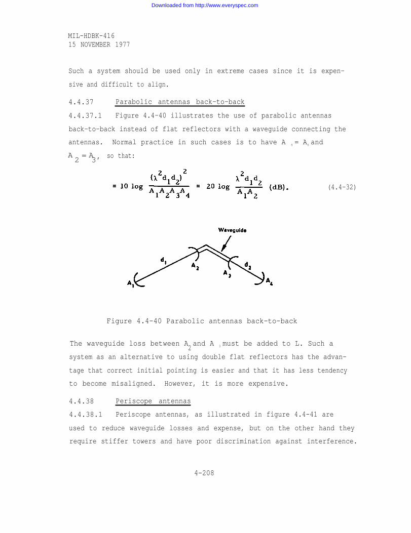
MIL-HDBK-41615 NOVEMBER 1977
Such a system should be used only in extreme cases since it is expen-
sive and difficult to align.
4.4.37 Parabolic antennas back-to-back
4.4.37.1 Figure 4.4-40 illustrates the use of parabolic antennas
back-to-back instead of flat reflectors with a waveguide connecting the
antennas. Normal practice in such cases is to have A 4 = A4 and
A = A2 3’
so that:
(4.4-32)
Figure 4.4-40 Parabolic antennas back-to-back
The waveguide loss between A and A 3 must be added to L. Such a2system as an alternative to using double flat reflectors has the advan-
tage that correct initial pointing is easier and that it has less tendency
to become misaligned. However, it is more expensive.
4.4.38 Periscope antennas
4.4.38.1 Periscope antennas, as illustrated in figure 4.4-41 are
used to reduce waveguide losses and expense, but on the other hand they
require stiffer towers and have poor discrimination against interference.
4-208
Downloaded from http://www.everyspec.com

MIL-HDBK-41615 NOVEMBER 1977
The reduced waveguide losses make this system especially attractive
between 15 and 40 GHz.
Figure 4.4-41 Periscope antenna
4.4.38.2 The reflector is in the near-field region of the antenna, and
its theoretical maximum gain is 6 dB above the gain of the dish.
Practical sizes of antenna and reflector limit this figure to 2 tO 3 dB,
and the area of the reflector should be more than twice that of the
parabolic antenna. The performance also varies with the wavelength
and with the distance between the reflector and the antenna.
4.4.39 Diffractors as passive repeaters
4.4. 39.1 Performance on paths with a diffracting mountain obstacle
can sometimes be improved by a diffraction grating screen. Such a
procedure is especially useful at higher frequencies (11 GHz) where
large, truly flat reflectors are expensive and difficult to construct.
The diffractor is a microwave version of the optical Fresnel lens, and
there are two types -- the screen type and the dielectric type. The
screen type acts by blocking off the wave components which would
cancel the received field, while the dielectric type shifts their phase to
add to the received field. They are placed on the ridge forming the com-
mon horizon for a diffraction path, and provide effective gain over the
natural obstacle.
4-209
Downloaded from http://www.everyspec.com

MIL-HDBK-41615 NOVEMBER 1977
4.4. 39.2 Figure 4.4-42 shows the position of the diffractor on the
ridge. Since the dielectric type is more efficient than the screen type,
it can be made considerably smaller. The diffractor does not need to be
on the great circle path between sites.
Figure 4.4-42 Microwave diffractor
The gains corresponding to aperture area associated with flat reflec-
tors may be applied to the diffractor or lens type passive repeater.
4.4.40 RF transmission lines
4.4.40.1 There are two general classes of transmission lines which
are used for LOS radio links, coaxial cable and waveguide. Other
types such as two-wire lines and dielectric waveguide are never used.
Coaxial cable and waveguide will be discussed separately.
4.4.41 Coaxial cable
4.4. 41.1 As the state-of-the-art of radio communication has
advanced over the past several decades, numerous types of coaxial
line have been developed to meet the requirements of system design.
The most important of these requirements for LOS radio links are
minimum line loss, and ease of installation. The major types of
4-210
Downloaded from http://www.everyspec.com

MIL-HDBK-41615 NOVEMBER 1977
interest are the air-dielectric rigid or flexible lines and foam-
dielectric flexible lines. Rigid lines which use dielectric beads to
support the center conductor are seldom used above 300 MHz due to
the difficulty of installation.
4.4.41.2 At moderate frequencies, say up to 2 or 3 GHz, flexible
coaxial cables are used for both transmitter and receiver lines. The
available separators for diameters of interest include a helical plastic
strip between inner and outer conductors, solid dielectric and foamed
plastic dielectrics. These cables are easily installed in continuous
runs from the RF equipment to the antennas and are available with
factor y-installed fittings. Field installation of fittings should be avoided
where at all possible. Most field fittings are mechanical and electrical
compromise solutions to a problem which is much more effectively
handled in a factory where proper tools and materials and trained
craftsmen are available.
4.4.41.3 Pressurization of transmission lines is used except with
solid or foam dielectric lines in order to keep moisture out of the line
since water between the conductors and corrosion of the conductors will
greatly increase line loss O
4.4.41.4 Almost all flexible coaxial cables are covered with a thick
sheath of tough plastic which is an important element in the mechanical
structure of the line. This sheath may be removed from the line to
provide an electrical ground connection but since this weakens the
entire structure, it should be avoided. If this is done on bends, it
may cause the line to kink where the sheath has been removed.
4.4.41.5 Although coaxial lines are inherently broad-band devices,
large diameter lines are unsuitable at high frequencies, since wave-
guide modes may be excited which extract power from and interfere
4-211
Downloaded from http://www.everyspec.com
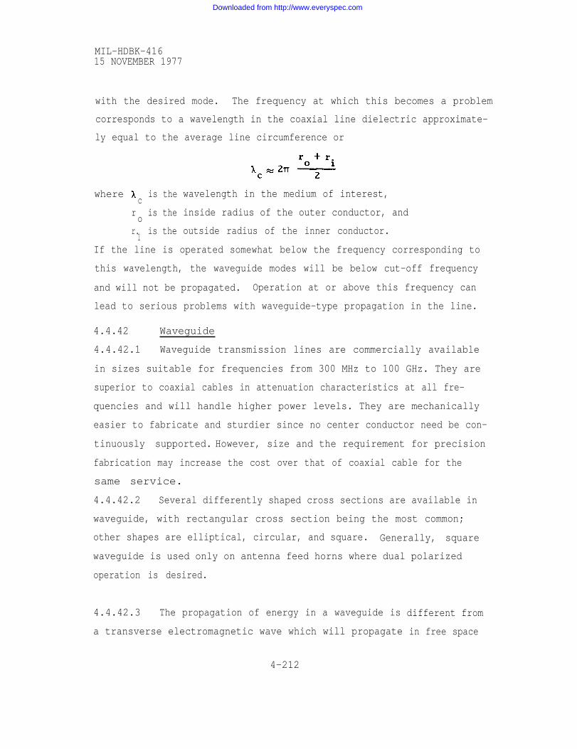
MIL-HDBK-41615 NOVEMBER 1977
with the desired mode. The frequency at which this becomes a problem
corresponds to a wavelength in the coaxial line dielectric approximate-
ly equal to the average line circumference or
where is thec
r is theo
r. is the1
wavelength in the medium of interest,
inside radius of the outer conductor, and
outside radius of the inner conductor.
If the line is operated somewhat below the frequency corresponding to
this wavelength, the waveguide modes will be below cut-off frequency
and will not be propagated. Operation at or above this frequency can
lead to serious problems with waveguide-type propagation in the line.
4.4.42 Waveguide
4.4.42.1 Waveguide transmission lines are commercially available
in sizes suitable for frequencies from 300 MHz to 100 GHz. They are
superior to coaxial cables in attenuation characteristics at all fre-
quencies and will handle higher power levels. They are mechanically
easier to fabricate and sturdier since no center conductor need be con-
tinuously supported. However, size and the requirement for precision
fabrication may increase the cost over that of coaxial cable for the
same service.
4.4.42.2 Several differently shaped cross sections are available in
waveguide, with rectangular cross section being the most common;
other shapes are elliptical, circular, and square. Generally, square
waveguide is used only on antenna feed horns where dual polarized
operation is desired.
4.4.42.3 The propagation of energy in a waveguide is
a transverse electromagnetic wave which will propagate
different from
in free space
4-212
Downloaded from http://www.everyspec.com

MIL-HDBK-41615 NOVEMBER 1977
or in a coaxial line. All wave guide modes exhibit a field component in
the direction of propagation. If this component, in the direction of
propagation is magnetic, the mode is called a TE (transverse electric)
mode; if the component in the direction of propagation is electric the
mode is called a TM (transverse magnetic) mode. The individual
modes are identified by dual subscripts as, for example, a TE2, 1
mode.
4.4.42.4 In constrast to a coaxial line which can be used for any
frequency from dc to that where waveguide modes becomes possible, a
wave guide has a low-frequency cutoff below which propagation will
not occur in any mode. In a rectangular guide, the wavelength of the
cutt-off frequency is given by
= 2ac
where a is the inside width of the broad wall of the wave guide l
4.4.42.5 For waveguide of elliptical cross-section, the cutoff wave -
length depends on the ratio of major-to-minor axes and can be obtained
from manufacturers data. For a typical ellipticity of O. 75, it can be
said generally that it exceeds the cutoff wavelength of a rectangular
waveguide circumscribing the ellipse.
4.4.42.6 At frequencies much above the fundamental cut-off fre-
quency other waveguide modes will propagate. It is desirable to have
only the fundamental mode present so there is a range of frequencies
over which a particular size of waveguide is used. These ranges are
specified by the manufacturer.
4.4.42.7 The return loss and VSWR of waveguide lines are strongly
influenced by the regularity of the waveguide cross section. For this
reason, great care must be taken to prevent deformation of the wave-
guide during installation or inspection. This is particularly important
4-213
Downloaded from http://www.everyspec.com

MIL-HDBK-41615 NOVEMBER 1977
where long lengths of semi-flexible elliptical waveguides are used
since just one kink or crush will ruin a long expensive piece of wave -
guide. For continuous-length waveguides, field fitted connectors
should be avoided. It is very difficult to find field personnel who can
consistently produce a mechanically and electrically adequate connector
installation. If field-fitted connectors are used, great care must be
taken and frequent inspections made by a qualified craftsman to insure
an adequate job.
4.4.42.8 In addition to long lengths of semi-flexible elliptical wave-
guide or 20 -foot lengths of rigid rectangular guide, other waveguide
pieces are necessary. These include 45° and 90° bends in both polari-0
zation planes, 45 and 90° twists, short lengths of flexible twistable
guide, and wave guide-to-coaxial adapters. Other components made
from rigid rectangular guide are available or can be made up. These
components are desirable to complete a waveguide installation at the
antenna and equipment connections.
4.4.42.9 If an antenna is to be used for both horizontal and vertical
polarization, two waveguide runs are generally necessary between
antenna and equipment. The signals are combined in a square wave-
guide polarization filter which is part of the antenna feed horn assembly.
The isolation between signals of orthogonal polarization in such a
systerm should be 50 to 60 dB.
4.4.42.10 Figure 4.4-43 shows typical attenuation, and range of
single mode use of various waveguide transmission lines.
4.4.43 Microwave separating and combining elements
4.4.43.1 By means of separating/combining networks, groups of
several transmitters and several receivers are connected to the same
antenna. For determining circulator and/or diplexer network losses, the manu-
facturer's specifications should be checked. For new equipment, these losses
should seldom exceed 1 dB.
4-214
Downloaded from http://www.everyspec.com

MIL-HDBK-41615 NOVEMBER 1977
Figure 4.4-43 Microwave Waveguide Attenuation
4-215
Downloaded from http://www.everyspec.com

MIL-HDBK-41615 NOVEMBER 1977
4.4.43.2 The following list of such networks may be incomplete but
it contains customary and recommended types for application in radio
relay engineering.
a. Circulator Networks (figure 4.4-44). - These are, for
instance, three-armed circulators, one arm of which is connected to a
filter, while another is connected to a neighboring circulator (or a
termination) and a third arm is connected to another neighboring circu-
lator (or the antenna feeder). The interconnection of a circulator and a
filter is a separating/ combining filter element.
b. Bridge-type Networks (figures 4.4-45a and 4.4-45b) -
These consist of filter networks and four-arm bridge elements such as
3 dB directional couplers or "magic tees". TwO bridge elements are
connected by two equal filters to produce a separating-filter element.
Of the four terminals of a separating-filter element one is connected to
the equipment terminal, another to a termination; the two remaining
ones are connected to neighboring separating-filter elements or one of
the two terminals is connected to the antenna lead or a termination.
c. Branching Networks (figure 4. 4-46). - These networks
consist of filters whose inputs or outputs are connected in parallel.
d. Polarization Filters (figure 4. 4-47). - Polarization
filters have two terminals for rectangular waveguide going to the trans -
mitters or receivers and one terminal for circular or square wave-
guide going to the antenna.
4.4.44 Transmitters
4.4.44.1 Figure 4.4-48 is a block diagram of a typical radio relay
transmitter. The transmitter for a frequency-modulation system
normally comprises of a baseband group, modulator, oscillator, trans-
mit mixer, and radio-frequency amplifier. In direct-modulation
4-216
Downloaded from http://www.everyspec.com

MIL-HDBK-41615 NOVEMBER 1977
Figure 4.4-44 Circulator Networks
Figure 4.4-45a
Figure 4.4-45b
Figure 4.4-46 BranchingNetworks
Ant.= antennaA = terminationIS = isolatorLP = lowpass filtcrBP = bandpass filtcr
Filters
BS = bandstop filterc = circulatorBE = bridge elementPF = polarization filterTl = equipment terminals
4-217
Figure 4.4-47 Polarization
Downloaded from http://www.everyspec.com

MIL-HDBK-41615 NOVEMBER 1977
Figure 4.4-48 Block Diagram of Typical Microwave Transmitter
4-218
Downloaded from http://www.everyspec.com

MIL-HDBK-41615 NOVEMBER 1977
systems, the oscillator which operates at the radio-frequency is
directly modulated in frequency, and the transmit mixer is omitted.
4.4.44.2 The Baseband Group includes a pilot oscillator and pilot
tone detector for alarm functions, pre-emphasis networks, and an
insertion amplifier.
4.4.44.3 Modulation. - The design and efficiency of radio-relay
equipment is determined chiefly by the type of modulation used. The
various types of modulation eligible for radio-relay systems are
essentially:
a. Frequency-modulation,
b. Pulse-modulation (pulse -code modulation).
4.4.44.4 Frequency modulation is most widely used in radio-relay
equipment and it is the only type commonly used at present for broad-
band systems. The following considerations therefore apply to
frequency-modulation systems.
4.4.44.5 The generation of microwave frequencies with high accura-
cy and stability is possible both with free-running oscillators (e. g. ,
klystrons and solid-state components) or with crystal oscillators and
subsequent multiplication. A disadvantage of the free-running micro-
wave oscillators is their comparatively large frequency-drift because
of variations in the ambient temperature and in the supply voltages.
The frequency therefore must be maintained constant by means of an
automatic frequency-control circuit. Either a highly temperature
compensated resonator or a harmonic of a crystal-controlled lower
frequency is used as a reference for automatic frequency control.
4.4.44.6 When the microwave frequency is produced by multiplying a
crystal-controlled oscillation, harmonic mode crystals (mostly around
100 MHz) are customarily used to reduce the number of multiplier
stages. Multiplication formerly was made exclusively by means of
4-219
Downloaded from http://www.everyspec.com

MIL-HDBK-41615 NOVERBER 1977
tubes, but today semi-conductors (variable capacitance diodes, or
step-recovery diodes) are used. At the output of the multiplier not
only the desired frequency but also other harmonics of the fundamental
frequency appear, and these must be suppressed by filters. Moreover,
the noise problem needs particular consideration in this case due to
spurious responses in some of the diodes.
4.4.44.7 RF transmitter power values required in microwave Sys-
terns range from 100 mW to 15 W, depending on the frequency and on
the respective transmission capacity. The RF power may be produced
by klystrons,traveling-wave tubes, or solid-state devices. The power
stage must be followed by an output filter in order to suppress harmon-
ics and spurious radiations (approximately by 60 dB).
4.4.44.8 The power amplifier is one module which can be changed
without affecting the basic design of the transmitter, There are com-
mercially available solid-state power amplifiers with 1 W output up to
15 GHz. In the past, power amplifiers were one of the weakest links
in the reliability chain because they required hot-filament devices.
Extremely reliable transmitters make it possible to place the RF
stages near the antennas on the towers. Thereby the requirements for
long RF transmission lines are eliminated and accompanying losses and
feeder echo distortion are reduced. Also the requirement for a hot stand-
by transmitter on space diversity systems is alleviated. RF equipment may
still have to be placed at the base of towers at sites where modulation and
demodulation is required, but if modulators and demodulators are available
with improved reliability, all microwave components may be mounted on
the tower even in such cases.
4.4.44.9 The development of a transmission device called an
injection-locked oscillator which allows the translation of microwave
frequencies while retaining the modulation with very little distortion
eliminates many microwave components and may supersede the
4-220
Downloaded from http://www.everyspec.com

MIL-HDBK-41615 NOVEMBER 1977
conventional transmitter and much of the receiver at sites where form-
erly heterodyne repeaters would have been installed. For power levels
of 10 W and greater, traveling-wave tube amplifiers will continue to be
used for sometime since the reliability of such devices continues to
improve.
4.4.44.10 A large variety of arrangements of components and types of
components exists and others are being developed. Transmitters for
a specific system will probably be selected under one single equipment
specification stipulating such overall quality considerations as carrier
frequency stability, levels, group delay, linearity, modulator linear
deviation range, output carrier-to-noise ratio, and minimum noise
power ratio.
4.4.45 Receivers
4.4.45.1 As in the case of transmitters, a large variety of component
arrangements and types may be used in a commercial receiver and
many others are being developed. A block diagram of a typical micro-
wave receiver is shown in figure 4.4-49. Though not shown in the
block diagram of the receiver, sensing and alarm functions are integral
to all microwave communications systems.
4.4.45.2 A frequency modulation microwave receiver which, in
general, operates on the superheterodyne principle consists essentially
of a radio-frequency input filter, mixer, oscillator, intermediate -
frequency amplifier, limiter, discriminator, and baseband group.
4.4.45.3 The radio-frequency input filter suppresses unwanted
frequencies outside the band to be received (particularly image
frequencies), and at the same time prevents unwanted spurious emis-
sions of the oscillator frequency and of mixing products.
4.4.45.4 In the mixer, which is mostly made up of semi-conductor
diodes, the arriving radio-frequency signal must be translated into the
4-221
Downloaded from http://www.everyspec.com
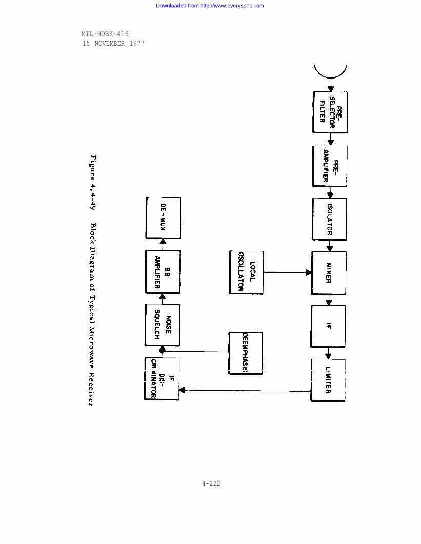
Figure 4.4-49
MIL-HDBK-41615 NOVEMBER 1977
4-222
Downloaded from http://www.everyspec.com

MIL-HDBK-41615 NOVEMBER 1977
intermediate-frequency (IF) band with as little noise as possible being
produced. With presently available diode mixers, a receiver noise
figure of 8 to 9 dB at 1 GHz and of 10 dB at 7 GHz can be obtained. “
Better noise figures are possible using tunnel-diode amplifiers,
parametric amplifiers, and molecular amplifiers; the latter are used
however primarily for communication-satellite systems since external
noise contributions with terrestrial systems negate the advantages of
extremely low internal noise figures.
4.4.45.5 The principles applicable to the transmitting oscillators
apply equally to the production of the receiving oscillator frequency.
4.4.45.6 The intermediate-frequency amplifier must have a gain of
approximately 70 dB; to compensate for varying path losses it must
also have an automatic gain control with a range of at least 40 dB.
Since a high freedom from distortion is required, especially in broad-
band systems, appropriate measures must be taken to provide ampli-
tude and delay equalization.
4.4.45.7 In the subsequent limiter, the synchronous amplitude -
modulation superimposed on the frequency-modulated signal must be
eliminated as far as possible.
4.4.45.8 The discriminator which demodulates the intermediate-
frequency signal must meet high requirements with respect to freedom
from distortion, especially in broadband transmission.
4.4.45.9 The receiver baseband group includes a pilot detector,
noise limiting circuitry, a baseband amplifier, filters, and demulti-
plexing equipment.
4.4.45.10 In systems with through-connection at intermediate
frequencies, the limiter, discriminator, and baseband circuits are
packaged together with the modulator in the modulator equipment
housing which is required at terminal stations only.
4-223
Downloaded from http://www.everyspec.com

MIL-HDBK-41615 NOVEMBER 1977
4.4.45.11 In operation,a signal from the antenna passes through a
ferrite isolator which reduces intermodulation noise. The signal then
passes through a waveguide preselector filter that provides a high IF
image injection ratio and eliminates interference from adjacent RF
channels. The signal is then mixed with the local oscillator output to
produce the 70 MHz IF frequency. The IF output is amplitude limited
and the limiter output is applied to a frequency discriminator, a de-
emphasis circuit, and a noise muting or squelch circuit that disconnects
the baseband amplifier and demultiplexing equipment if system noise
increases above a pre-set level. After the squelch circuit, the signal
is passed to the baseband amplifier and then to the demultiplexing
equipment where the original intelligence is retrieved.
4.4.45.12 Some of the overall receiver equipment specifications
which determine its quality are noise figure, local oscillator frequency
stability, discriminator linear range, group delay linearity, amplitude
linearity, and the minimum noise power ratio it is capable of providing.
A preamplifier may be added or removed without changing the basic
design of the receiver. If a suitable low-noise preamplifier is placed
at the antenna end of a required long transmission line, line loss no
longer degrades the carrier-to-noise ratio. Therefore, not only can
additional receiver sensitivity be gained but the effects of line loss can
be removed.For microwave radio relays low-noise microwave pre-
amplifiers are usually the tunnel diode type. These amplifiers become
nonlinear at relatively low received carrier levels (-50 to -40 dBm).
Because of this gain nonlinearity and the sensitivity of amplifier gain
to operating temperature, the following precautions should be taken
when using tunnel diode amplifiers:
a. A preselector filter should be placed between the
antenna terminal and the preamplifier input so that
abnormally high unwanted signal levels can be avoided.
4-224
Downloaded from http://www.everyspec.com

MIL-HDBK-41615 NOVEMBER 1977
b. Since the gain characteristics of tunnel diode preampli-
fiers are usually affected by temperature and they are
often mounted external to the equipment shelter, a
small compartment capable of protecting the preampli-
fier from weather and having reliable thermostatic
temperature control should be supplied.
c. The input to the preamplifier is the location most
susceptible to interference.
4.4.45.13 Figure 4.4-50 shows preamplifier noise figures as a func-
tion of carrier frequency. These values are based on equipment avail-
able at this time. As already noted, noise figures of receivers not
using preamplifiers run higher and are typically as follows:
Noise Figure Frequency Range
10 dB 1 to 10 GHz
12 dB 10 to 36 GHz
4.4.46 Active repeaters
4.4.46.1 An active repeater must be able to perform at least three
essential functions. It must (1) provide gain (up to approximately
110 dB), (2) change the direction of microwave route if required, and
(3) be able to change the carrier frequency slightly to minimize intra-
system interference. (252 MHz is the common frequency shift). There
are basically two types of active repeaters, the demodulating type and
the non-demodulating type.
4.4.46.2 For an FM/FDM system, a block diagram for a typical
demodulating active repeater is shown in figure 4.4-51. Its advantages
are mainly flexibility and (at the time of this writing) lower cost. The
whole baseband is available allowing channels to be dropped or inserted
in an efficient manner.The equipment price advantage occurs as a
4-225
Downloaded from http://www.everyspec.com

MIL-HDBK-41615 NOVEMBER 1977
Figure 4.4-50 Nominal Noise Figures for Solid State ReceiverPreamplifiers Commercially Available
4-226
Downloaded from http://www.everyspec.com

Figure 4.4-51
MIL-HDBK-41615 NOVEMBER 1977
4-227
Downloaded from http://www.everyspec.com

MIL-HDBK-41615 NOVEMBER 1977
result of the manner in which gain is achieved; usually all of the
repeater gain is obtained at the intermediate frequency and in the
modulation - demodulation process. The disadvantages of the demodu-
lating repeater are:
a.
b.
c.
It usually introduces more noise per hop than a non-
demodulating repeater, but not when pulse code modula-
tion is used and the pulses are regenerated at each
repeater site.
Baseband levels tend to be less stable because level
variations occur primarily in the modulation and de-
modulation processes. These variations tend to be
cumulative in the system.
The maintenance of modulator and demodulator linear-
ity is critical for holding intermodulation noise to a
minimum. Thus, the cost of maintaining alignment
are often larger for the demodulating repeater than for
the non-demodulating type.
4.4.46.3 There are basically two types of non-demodulating repeat-
ers - RF and IF types. The RF heterodyne repeater obtains most of
its gain by using RF amplifiers, but such a procedure is expensive and
for this reason RF heterodyne repeaters are seldom used. RF repeat-
ers using injection-locked oscillators may come into greater usage
(see paragraph 4.4.44.9). The IF radio repeater is the most common non-
demodulating type, and a block diagram is shown in figure 4.4-52. This
repeater type obtains most of its gain at the intermediate frequency
which can be done cheaply and reliably with transistor amplifiers.
4.4.46.4 The choice of using through-connecting at repeater stations
(through-connection at baseband frequencies or at intermediate-
frequencies) is determined by technical possibilities (orderwire or
4-228
Downloaded from http://www.everyspec.com

Figure 4.4-52
MIL-HDBK-41615 NOVEMBER 1977
4-229
Downloaded from http://www.everyspec.com

MIL-HDBK-41615 NOVEMBER 1977
supervisory circuits) and by economic considerations as well as by the
traffic demands.
4.4.46.5 In systems using modulation at intermediate frequencies,
the baseband signal is converted into a FM standardized IF signal in
the modulator. In the RF equipment, this modulated IF is converted
into the final RF signal, and raised to the required level. At repeater
stations,through-connection can be made in the IF band. Since, in
this method, no modulators are used at repeater stations, the system
is free from the noise caused by nonlinearities in the demodulation, re-
modulation process.
4-230
Downloaded from http://www.everyspec.com

MIL-HDBK-41615 NOVEMBER 1977
Section 4.5 INTEGRATING LINK DESIGN INTO SYSTEM DESIGN
4.5.1 General
4.5.1.1 Tentative values for various link parameters are calculated
or selected using the information in section 4.4. These parameters
include antenna heights and separations, antenna types and gains,
transmission feeder line types and lengths, transmitter powers, and
receiver noise figures.
4.5.1.2 With these tentative values of equipment parameters selected
for individual links, they may be integrated into the system design.
Several checks and analyses must be completed to properly form the
links into a well designed system:
a.
b.
c.
d.
The system layout must be brought up to date with
current information which involves adding information
to system drawings and worksheets (section 4.5. 2).
Radio equipment block diagrams with associated
equipment requirement lists should be made for each
site (section 4.5.3).
Frequency compatibility must be assured. A frequency
plan must be completed (sections 4.5.4 through 4.5.7)
and an analysis of intrasystem interference must be
made (sections 4.5.8 through 4.5.13).
The tentative values of equipment parameters selected
on an individual link basis must be checked and
adjusted on the basis of total sys tern performance
(sections 4.5.14 through 4.5. 35). System perform-
ance predictions are made; on the basis of these pre-
dictions. Less reliable portions of the sys tern can be
changed to insure adequate overall noise performance
to established standards.
4-231
Downloaded from http://www.everyspec.com

MIL-HDBK-41615 NOVEMBER 1977
e. Finally, the total system design must be checked from
the standpoint of overall reliability (sections 4.5.36
through 4.5.40). System reliability cannot generally
be predicted accurately, but the system can be examined
for weak points.
4.5.2 System layout
4.5.2.1 A system layout with updated path, equipment, and perform-
ance parameter summaries should be prepared. This serves as a basis
for accurate system analyses and realistic cost estimates. The system
layout may simply be a line drawing on an outline map such as the
example in figure 4.5 -1. The drawing illustrates the general geo-
metric relationship between the sites and potential intra-system
interference problems. Although this figure
no attempt is made to analyze it specifically
4.5.2.2 To supplement the layout drawing,
worksheets are required:
represents a real system,
in this handbook.
three types of summary
a. a list of antenna locations with site codes, geographical
coordinates, and site elevation (worksheet 4. 5-1 a),
b. a list of parameters pertaining to the antennas and
their orientation to provide information for under-
standing the relationship between the terrain configura-
tion and the equipment requirements (worksheet
4.5-1 b), and
c, a summary of parameters for each
preparation of system performance
(worksheet 4.5-2).
path to facilitate
predictions
4-232
Downloaded from http://www.everyspec.com

MIL-HDBK-41615 NOVEMBER 1977
4-233
Downloaded from http://www.everyspec.com

MIL-HDBK-41615 NOVEMBER 1977
4-234
Downloaded from http://www.everyspec.com

. .
4-235
—
—
MIL-HDBK-41615 NOVEMBER 1977
Downloaded from http://www.everyspec.com

MIL-HDBK-41615 NOVEMBER 1977
4-236
Downloaded from http://www.everyspec.com

MIL-HDBK-41615 NOVEMBER 1977
4.5.3 Site radio equipment requirements
4.5.3.1 Requirements for equipment at each site should be summar-
ized in block diagrams which for simplicity should show the largest
subsystems which adequately define the radio equipment functions at
each site. Some subsystems may be broken down into more detailed
modules as required. Each block should be given a number, so that it
can easily be referred to in detailed breakdowns of equipment require-
ments. Descriptions of the various types of equipment in the block
diagram were given in section 4.4.28 through 4.4.45. Figure 4.5-2
is a typical example of a radio equipment block diagram for a site
being used not only as a repeater but also for branching and as a radio
terminal. Such a diagram would be much simpler for a site used only
as a repeater.
4.5.3.2 Two important uses of the block diagrams are:
a. they insure that each equipment component will be
considered individually and that none will be over-
looked, and
b. from the equipment lists, a realistic cost estimate
can be prepared in the form of lists and tables with
comments on each piece of equipment included in the
diagram. Some of the information in the comments
may concern military specification (if applicable),
manufacturers' and model number, cost, acquisition
lead time, insertion gain or loss, bandwidth, VSWR,
physical size, isolation, etc. The block diagram may
also be used to show some subsystem parameters such
as RF transmit and receive frequencies, transmitter
power, intrasite MUX channel routing, the path designa-
tion of the antenna, etc.
4-237
Downloaded from http://www.everyspec.com

MIL-HDBK-41615 NOVEMBER 1977
.
4-238
Downloaded from http://www.everyspec.com

MIL-HDBK-41615 NOVEMBER 1977
4.5.4 Frequency compatibility
4.5.4.1 Adherence to established national and international regulations
is essential to achieve interference free operation.
4.5.5 General aspects of frequency allocation
4.5.5.1 Within the frequency bands that are allotted to microwave
systems by international conventions, the C.C.I.R. has worked out
radio-frequency channel arrangements for the various systems indi-
cating the number, frequencies, and spacing of the RF channels that
can be used within the respective bands. Most of these arrangements
moreover contain recommendations regarding the number and prefer-
able polarization of the RF channels that may be carried over a common
antenna.
4.5.5.2 The provision of radio-frequency channel arrangements
indispensable considering the following objectives:
is
a.
b.
c.
d.
through-connection of microwave systems across
national borderlines;
prevention of mutual interference between neighbor-
ing countries in the border areas;
optimum utilization of the available RF spectrum;
prevention of mutual interference within countries
having great traffic densities.
4.5.6 References to appropriate sections of the Radio Regulations
4.5. 6.1 Article 3 of the Radio Regulations [99] provides general
rules for the assignment and use of frequencies; Article 4 provides
information on the conclusion of special agreements between two or
more Members or Associate Members of the I.T.U. regarding the
sub-allocation of bands of frequencies, and Article 5 sets out the allo -
cation throughout the world of frequency bands extending from 10 kHz
to 40 GHz,
4-239
Downloaded from http://www.everyspec.com

MIL-HDBK-41615 NOVEMBER 1977
4.5.6.2 Revisions to the Radio Regulations were made at the Extra-
ordinary Administrative Radio Conference in Geneva ( 1963) and a
resolution was drawn up relating to satellite systems and fixed and
mobile services in the frequency band 1525 to 1540 MHz. Recommenda -
tions relating to the sharing of frequency bands between communication-
satellite systems and terrestrial radio-relay systems were also
drawn up.
4.5.6.3 Of the recommendations adopted at the Extraordinary
Administrative Radio Conference, Geneva, Recommendation 1A relates
to the calculation of coordination distance. The C. C. I. R. have sub-
sequently studied further the problems associated with coordination
distance and, at the XIth Plenary Assembly at Oslo (1966), approved
Report 382 which deals with its determination [8 1].
4.5.7 Choice of one or more frequencies from those available inthe radio-frequency channel arrangement
4.5.7.1 Once a frequency band has been chosen, the individual
channel frequencies should always be arranged in accordance with
C. C. I. R. recommendations shown in table 4.5-1 and figure 4.5-3.
The frequency range is subdivided into two part S, the lower half of the
band and the upper half. These two halves are separated by a center
gap which is larger than, or equal to, the spacing between the center
frequencies of two adjacent channels. A frequency pair is designated
as f1, f'1, or f2, f'2, etc.
4.5.7.2 If the frequency spacing of a single pattern (preferred) has
been kept sufficiently large in relation to the modulation bandwidth, an
additional channel assignment may be made. The latter arrangement
is displaced by half the original channel spacing frequency, and may
be interleaved with the preferred arrangement. If dual arrangements
of this kind are employed, the mutual decoupling requirements must
be fulfilled.
4-240
Downloaded from http://www.everyspec.com

MIL-HDBK-41615 NOVEMBER 1977
4-241
Downloaded from http://www.everyspec.com
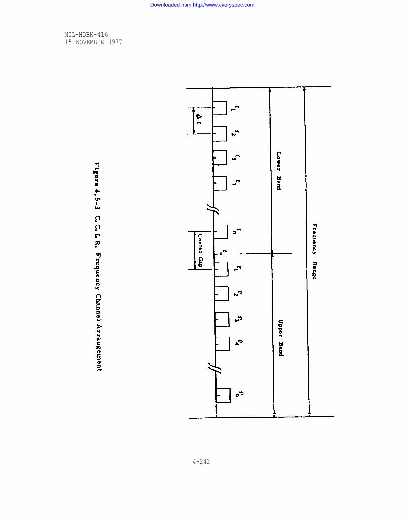
MIL-HDBK-41615 NOVEMBER 1977
4-242
Downloaded from http://www.everyspec.com

MIL-HDBK-41615 NOVEMBER 1977
4.5.7.3 Where two or more radio-frequency channels are to be pro-
vided over a route, frequencies should first be assigned either from
the odd-numbered group of channels or from the even-numbered group,
but not from both since this would require the use of two antennas at
each end of each section. As an example, when all the channels from
the odd-numbered group have been assigned, further expansion from
the even-numbered group would be provided by means of a second anten-
na with polarization orthogonal to that of the first antenna (see figures
4.5-4 and 4.5-5).
4.5.7.4 Figures 4.5-4, 4.5-5, and 4.5-6 show how a full comple-
ment of channels can be arranged. If separate antennas are used to
transmit and receive, two will be required at each end of a section,
irrespective of the actual number of two-way channels to be provided
initially.
Figure 4.5-4 Single Polarization Antenna Arrangement for the 2 and
Note 1:
Note 2:
4 GHz Bands
S 1, 2, 3, and 4 are the CCIR preferred auxiliary channels, in order offrequency.Alternations of polarization in every two hops are available for reductionof overreach interference.
4-243
Downloaded from http://www.everyspec.com

MIL-HDBK-41615 NOVEMBER 1977
Figure 4.5-5 Bipolar Antenna Arrangements for the 6 GHz Band
Figure 4.5-6 Separate Transmit/Receive Bipolar Arrangement
for the 6 GHz Band
4-244
Downloaded from http://www.everyspec.com
MIL-HDBK-41615 NOVEMBER 1977
4.5.8 The production and the effects of unwanted couplings
4.5.8.1 In planning a radio system comprising any number of sec-
tions in tandem, the initial choice of whether a terminal station shall
transmit in the upper half of the frequency band and receive in the lower
half, or vice versa, is arbitrary, but once chosen this high/low fre-
quency pattern remains constant for any one station and any one fre-
quency band. When, however, a system is being planned to provide
an alternative route between two points which are already connected by
a radio-relay system, the high/low frequency pattern of the common
terminal station is already determined, and the pattern of the new
route must conform to this established pattern if it is to operate in the
same frequency band. This can be done by choosing the number of
repeater sections in the new route to be either odd or even, depending
on whether the number of sections in the original route is odd or even.
For example, if the original route contained four repeater sections,
the new route may contain two, four or six sections, but not three or
five (it is unlikely that fewer than four sections could be used since it
is reasonable to assume that the original route used the least number
of repeater sections for the distance involved).
4.5.8.2 Figure 4.5-7a shows an example of an unacceptable fre-
quency plan where stations A and B are each receiving signals in the
low and high halves of the band simultaneously, and consequently both
are required to transmit simultaneously in both halves of the band.
The direct path from station H to station B cannot be used and signals
between them must be
corrects the high/low
B, as shown in figure
ment of figure 4.5-7a
routed via station C. This re-routing action
frequency pattern at both station A and station
4.5-7b. Further deficiencies of the arrange-
are evident, namely:
4-245
Downloaded from http://www.everyspec.com
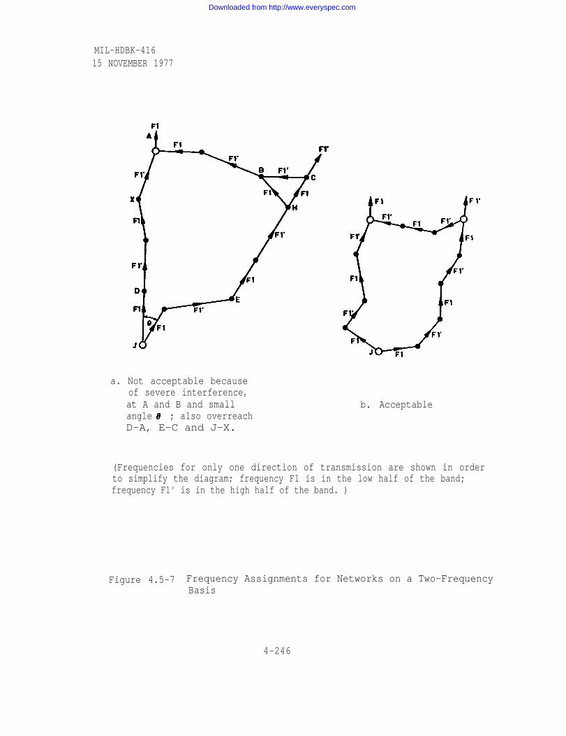
MIL-HDBK-41615 NOVEMBER 1977
a. Not acceptable becauseof severe interference,at A and B and smallangle ; also overreachD-A, E-C and J-X.
b. Acceptable
(Frequencies for only one direction of transmission are shown in orderto simplify the diagram; frequency F1 is in the low half of the band;frequency F1' is in the high half of the band. )
Figure 4.5-7 Frequency Assignments for Networks on a Two-FrequencyBasis
4-246
Downloaded from http://www.everyspec.com

MIL-HDBK-41615 NOVEMBER 1977
a. the angle between the two paths at J is too small and co-
channel interference would be experienced.
b. overreach signals from D to A, J to X and E to C could
occur, giving co-channel interference. The cure would
be to stagger the route so that the transmit antennas at
D, J and E do not point in the directions of A, X and C.
4.5.8.3 On very lightly loaded routes that are unlikely to expand,
i.e., those comprising only one or at the most two hi-directional radio- .
frequency channels, it may be possible by very careful selection of
frequencies to contravene this “rule” concerning the preservation of the
high/low frequency pattern. This could save the cost of one repeater
station, but if at some later date more channels in the same frequency
band were required, it would not be possible to provide them without
provision of the repeater station originally saved. To insert an extra
station into an existing route cannot be done without considerable diffi-
culty and cost and, inevitably, some dislocation to the traffic on the
route.
4.5.9 Types of interference
a. Co-channel Interference (Section 4.5.10)
This term refers to interference from a source, modu-
lated or otherwise, having essentially the same frequency as the wanted
carrier within expected stability limits. When the interference is
caused by the beat between two relatively high level carrier components
having a frequency separation which falls within the baseband of the
wanted
acter.
signal, the predominant interference will be single-tone in char-
When the carrier frequency separation falls outside the base-
band range of the wanted signal, and when the interference is from a
dispersed signal; the character of the interference will resemble that
of random noise.
4-247
Downloaded from http://www.everyspec.com
MIL-HDBK-41615 NOVEMBER 1977
b. Adjacent Channel Interference (Section 4.5.11)
This term refers to interference due to the presence
of one or more radio-frequency carriers, modulated or otherwise,
immediately adjacent in frequent y to that of the wanted modulated car-
rier. The term adjacent is normally taken as indicating the adjacent
channel in the frequency channeling plan which has been adopted.
c. Direct Adjacent Channel Channel Interference(Section 4.5.12)
As in case (b) above, this term refers to interference
due to the presence of adjacent carriers which may be present when
interference due to (b.) above has become negligible. The mechanism of
the interference, however, requires the interfering carrier to be
modulated.
d. Other Forms of Interference (Section 4.5.13)
This term refers to interference which can arise either
from external sources or from unwanted interactions within the radio
equipment such as, for example, the image response of the receiver.
4.5.10 Co-channel interference
4.5.10.1 Co-channel interference arises when there is excessive
interaction between signal sources operating on the same, or very
close frequencies. It is current practice to transmit a common carrier
frequency (Fl) from every alternate repeater station of a radio-relay
system. The remaining stations of the system transmit a second car-
rier frequency (F1') which differs from the first by an amount which
depends on the particular frequency plan employed (see
and 4.5-9). This arrangement can result
where station A transmitting on frequency
of station D, and vice versa (see figure 4.
such interference is normally provided by
in overreach interference
F1 illuminates the antenna
5-8). Protection against
careful site selection, and
by ensuring that sufficient antenna side-lobe suppression given by the
4-248
Downloaded from http://www.everyspec.com

MIL-HDBK-41615 NOVEMBER 1977
The ratio (wanted signal/interfering signal) depends on the gain of the antennas atangles relative to the gain in beam and difference of propagation lossesbetween main and overreach Paths l
Figure 4.5-8 Example of Overreach Interference
B. Results from insufficient front-to-back antenna discrimination.D. Results from a reflection from nearby trees, hill or building, etc., at point X
Figure 4.5-9 Example of Adjacent Station Interference
4-249
Downloaded from http://www.everyspec.com
MIL-HDBK-41615 NOVEMBER 1977
angles is provided. In difficult cases it may be possible to
provide additional protection by orthogonal polarization of the wanted
and unwanted signals. This is not always practicable if, for example,
a spur route branches off from one of the stations and it is desirable
to provide cross-polar discrimination between the main route and the
spur route. Interference may also be reduced by using an interleaved
frequency plan over a critical section. In such a plan all carrier fre-
quencies are changed in the same sense by an amount equal to half the
adjacent channel frequency spacing. This value is approximately 14.5
MHz in the 2 GHz, 4 GHz and 6 GHz bands when using standard
C.C.I.R. recommended frequency plans (see Recommendations 382-2
and 383-1 [81], or 20 MHz when using other C.C.I.R. frequency
plans (i.e., for 2700 telephone channels, 11 GHz systems, etc.).
4.5.10.2 Potential advantages of such an arrangement depend on the
channel baseband width in relation to the spacing of their carriers, and
also on the relative carrier levels. It is generally desirable to use a
carrier frequency spacing of not less than three times the highest
baseband frequency so that the first-order sidebands of one channel do
not overlap the second-order sidebands of the other channel. Closer
spacings in terms of multiples of the highest baseband frequency may
be used with care, depending on the relative levels of the wanted and
unwanted carriers and the degree of interference that is acceptable.
4.5.10.3 A further interference mechanism can be seen in figure
4.5-9 where radiation at frequency F1' from the back of the antenna
at station B is received at station A. Even when the front-to-back dis-
crimination of the antenna is sufficient (at least 65 dB) to reduce this
interference to an acceptable level, reflections from nearby objects
can cause problems as shown at station D (figure 4.5-9). Reduction
of this type of interference can be achieved either by antennas of
4-250
Downloaded from http://www.everyspec.com

MIL-HDBK-41615 NOVEMBER 1977
improved directivity (including less radiation from side lobes), by the
use of a more suitable site, or possibly by the use of an interleaved
frequency plan.
4.5.10.4 Figure 4.5-10 shows an example of interference from a spur
or crossing which is similar to that shown in figure 4.5-9 (case D)
except that here no reflection need to be involved and the relative gain
of side lobes controls the interference level. If, on the main route,
signals of the same frequency arriving from opposite directions are of
the same polarization, the spur route can be cross-polarized with
respect to both directions. If, however, the main route signals are
cross-polarized (and there is not necessarily any advantage in this),
the spur route should be cross-polarized with respect to the direction
with the least angular separation.
4.5.10.5 In some cases it may be possible to reduce the effects of co-
channel interference by applying dispersal to the unwanted signal. Dis-
persal involves phase-deviating the carrier by several radians at a
The ratio (wanted signal/interfering signal) will depend on the front-to-sidediscrimination of the antennas X and Y.
Figure 4.5-10 Example of Spur Route Interference
4-251
Downloaded from http://www.everyspec.com

MIL-HDBK-41615 NOVEMBER 1977
slow rate and spreads interference over many channels at reduced
levels which would otherwise affect a few telephone channels at higher
levels. The reduction in interference is most pronounced in the lower
frequency channels which are subject to the highest interference levels
which are those caused by the beat tone between the wanted and un-
wanted residual carriers.
4.5.11 Adjacent channel interference
4.5.11.1 Adjacent channel interference can arise when (for a given
baseband width and adjacent carrier separation) suppression of the
adjacent carrier and overlapping unwanted sidebands is inadequate.
The reduction of interference from this source to an acceptable level
depends upon several factors. First, adequate separation of the adja-
cent channel spectra must be provided, and this is taken into account
in the radio-frequency channel arrangements recommended by the
C.C.I.R. Second, adequate RF and IF selectivity must be provided to
reduce the level of unwanted adjacent spectra. In providing such
filtering the equipment designer must take into account the possibility
of introducing distortion into the wanted signal path. Third, cross-
polarized discrimination between adjacent channels should be used to
supplement the selectivity provided by filtering. Cross-polarization
discrimination of some 25 to 30 dB is both practical and necessary.
4.5.12 Direct adjacent channel interference
4.5.12.1 Direct adjacent channel interference arises when the wanted
and unwanted signals are together subjected to amplitude limiting. It
is believed that partial conversion to amplitude modulation of the un-
wanted frequency-modulated signal takes place on the selectivity
skirts of the wanted channel. This amplitude modulation is demodu-
lated in the limiter of the wanted channel, demodulates the wanted
signal, and appears at the discriminator output along with the wanted
4-252
Downloaded from http://www.everyspec.com

MIL-HDBK-41615 NOVEMBER 1977
signal. The end effect is intelligible crosstalk, and the level of the
interference varies by 2 dB for each 1 dB variation in the wanted-to-
unwanted carrier ratio. Interference from this source may be reduced
to acceptable levels by proper equipment design. Together with the
cross-polarization
selectivity must be
discrimination between adjacent channels, adequate
provided prior to limiting.
4.5.13 Other sources of interference
4.5.13.1 Interference can occur within a system as a result of defi-
ciencies in the equipment itself. For example, a superheterodyne
receiver has several sensitive regions at which interference can be
received, namely:
Frequency differential betweenreceived signal frequency andmultiples of the IF
0; ±1/2 IF
± l IF
Sensitive region
Channel carrier frequency
Local oscillator frequency andimage frequency
± 2 IF
± 3 IF
4.5.13.2 Adequate selectivity prior to the low-level mixer is neces-
sary to desensitize the receiver in all regions but that of the channel
carrier frequency.
4.5.13.3 The designer must also ensure that the outputs of all local
oscillators are of high spectral purity; i.e., as free as possible from
spurious signals, random noise and both long-term and short-term
frequency changes. Spurious signals in local oscillators can arise
4-253
Downloaded from http://www.everyspec.com
MIL-HDBK-41615 NOVEMBER 1977
from imperfections of the crystal itself, inadequate filtering of unde-
sired crystal harmonics or self-oscillation, and general instability in
varactor multiplier chains.
4.5.13.4 A further interference mechanism exists on systems which
employ common antennas and feeders to transmit and receive more
than one frequency band. All wave guide feeders exhibit amplitude non-
linearity to some extent, mainly resulting from imperfections at
joints. Such non-linear elements result in intermodulation between
the outputs of two or more transmitters, and the resulting unwanted
products may fall close to receive frequencies either in the same fre-
quency band or in a different frequency band from that of the originat-
ing transmit channels. A careful selection of associated frequencies
and quality control of the waveguide joints is required to avoid the
worst effects.
4.5.14 Hop/System noise performance estimates.
4.5.14.1 Required performance levels are described in the following
paragraphs.
4.5.15 DCS noise requirements.
4.5.15.1 Once the link and system lengths are fixed, the total
median noise allocation can be calculated. A useful figure is to allow
3 pWO of voice channel noise per kilometer of actual system length; that
is, the sum of all individual path length (see [3], p22). This figure
is an approachable and probably realizable number. This basic assumptions
for noise allocations is that for long systems (say 1,000 to 10,000 km),
the total noise will remain within the allowable limits. Some individual
hops may have more median noise than allocable and some less.
4.5.16 Calculate hop noise allowance.
4.5.16.1 Initial calculation procedures are illustrated by an example.
Consider the system shown in figure 4.5.11. Sites 1, 4, 7, and 9 are
terminal locations where the FM signal in modulated from and
4-254
Downloaded from http://www.everyspec.com

Figure 4.5-11
MIL-HDBK-41615 NOVEMBER 1977
4-255
Downloaded from http://www.everyspec.com

MIL-HDBK-41615 NOVEMBER 1977
demodulated to baseband. At this stage of the design, we need not be
concerned if the baseband is built up from or broken down to voice
channels, groups or super groups at these locations, since multiplex
noise will be evaluated at a later point in the design.
4.5.16.2 Sites 2, 3, 5, 6, and 8 are repeater locations. In our
example, heterodyne repeaters are assumed since their noise contri-
bution is lower than that from baseband repeaters.
4.5.16.3 Presumably, traffic density studies, frequency plans, and
preliminary equipment parameter selection have been made.
4.5.16.4 For purposes of the example, assume that 600 voice channels
are required between sites 1 and 9 using an FM-FDM system operating
in the 7.125 to 8.400 GHz band. Two other parameters may now be
considered, receiver noise figure and per-channel deviation, If equip-
ment on hand is to be used, obtain these numbers from operations and
maintenance records. If new equipment is to be used, obtain values
from the manufacturers published figures. If none of these figures
are available, refer to paragraph 4.4.45.13 for a realizable receiver
noise figure and select a value of per channel or peak carrier devia-
tion from table 4.5-2. For example, a 10 dB noise figure and 200 kHz
per channel RMS deviation fixes the IF bandwidth at 20 MHz.
4.5.16.5 With these equipment and operating parameters we may
proceed with the system calculations. The total length of the system
is 300 kilometers (sum of the individual hop lengths). The total noise
allowance (excluding multiplex and through-group or through-
supergroup noise is therefore 900 pWO for this section (3 pWO per km).
4.5.16.6 Next one-eighth of the total noise is allocated to each of the
eight radio hops. This simple procedure is used because there will
not be any appreciably different thermal noise between longer and
shorter hops since each will be designed to have a received signal
4-256
Downloaded from http://www.everyspec.com

TABLE 4.5-2
MIL-HDBK-41615 NOVEMBER 1977
4-257
Downloaded from http://www.everyspec.com

MIL-HDBK-41615 NOVEMBER 1977
level (in our example) of approximately -27.5 dBm by appropriate
choice of antenna size and other equipment parameters. The inter-
modulation noise contributions will also be a function of the equipment
used (baseband repeater, IF repeater, heterodyne repeater) and will
therefore be fixed regardless of hop length.
4.5.16.7 The thermal noise for each hop can be determined from
figure 4.5-12 for the selected system parameters and entered on
worksheet 4.5-3. This value is 12.5 pWO for each hop based on the
choice of -27.5 dBm received signal level and a 600- channel system.
4.5.16.8 The equipment intermodulation plus basic noise allocation
is considered in section 4.5.20. For the example, assuming dual diversity
with equal gain combiners, there is 45 pWO intermodulation noise for a
heterodyne repeater-to-heterodyne repeater hop and 113.5 pWO for a terminal-
to-heterodyne repeater hop. Thus, hop A will contribute 113.5 pWO, B will
contribute 45 pWO, etc. Such values are also entered in worksheet 4.5-3.
4.5.16.9 Feeder echo intermodulation noise contribution is somewhat
more difficult to calculate, but 10 pWO is a useful first estimate for
well-designed and carefully installed transmission lines of average
length. The links as finally designed will no doubt differ somewhat
from this first cut estimate. The 10 pWO value is also entered in
worksheet 4.5-3 for each hop.
4.5.16,10 Total noise expected on each hop is the sum of the individual
contributions, and the total predicted system noise is the sum of the
contributions from each hop; this is compared with the total noise
allocated. In the example the calculated noise is somewhat greater than
the total allocated; thus, an attempt should be made to reduce each of
the individual hop contributions either by selection of different
equipments to reduce equipment intermodulation noise, by increasing
signal levels to reduce thermal noise (while bearing in mind that too4-258
Downloaded from http://www.everyspec.com

MIL-HDBK-41615 NOVEMBER 1977
Figure 4.5-12 Thermal Noise versus Received Signal Level
4-259
Downloaded from http://www.everyspec.com

MIL-HDBK-41615 NOVEMBER 1977
4-260
Downloaded from http://www.everyspec.com

MIL-HDBK-41615 NOVEMBER 1977
great a signal increase can result in increased intermodulation
distortion ), or by assuming lower feeder echo intermodulation
noise ( which may necessitate the use of tuned lines or several
load isolators ).
4.5.17 Select basic equipment parameters
4. 5.17.1 Figure 4.5-13 illustrates qualitatively the effects on
system performance ( in terms of the voice channel signal-to-
noise ratio ) of varying frequency deviation, noise power ratio,
and receiver noise figure. The arrows indicate the effects of
increasing these parameters. The effect of increasing feeder
echo intermodulation noise is the same as decreasing the noise
power ratio. Using the methods of this section, quieting curves
can be drawn for each hop for different assumed values of these
parameters.
4. 5.17.2 The foregoing calculations have been made to establish
the permitted long-term ( median ) voice channel noise. The
short-term voice channel noise, in accordance with current mili-
tary standards, is allocated on a per-hop basis, and shall not
exceed 316, 000 pWpO for more than an accumulated two minutes
in any month, or more than one minute in any hour as measured
with an amplitude distribution analyzer having an integration time
of 5 ms ( see MI L-ST D-188-313 ). As always, appropriate
military standards and DCA circulars ( see paragraph 1.1.1)
must be consulted when designing part of the DCS system. Methods
for estimating short-term noise will be described in the following
sections. However, a somewhat more stringent requirement based
on flat weighting will be used for simplicity, namely a short-term
noise level limited to 1, 000, 000 pWO which must not be exceeded
for 2 minutes per year, i. e. , the noise level must be less than
4-261
Downloaded from http://www.everyspec.com

MIL-HDBK-41615 NOVEMBER 1977
Figure 4.5- 13 Effect of Parameter Variation onTransfer Characteristics
4-262
Downloaded from http://www.everyspec.com

15 NOVEMBER 1977MIL-HDBK-416
1,000,000 pWO for 99.9995% of the year. This requirement
is at least equal and actually more stringent than that implied
by the military standards. Although the allowable noise power
is greater in the method given here ( 316,000 pWpO 500,000 pWO),
the allowable time during which this value may be exceeded is
much shorter.
4.5.17.3 After completion of the initial noise objective calcu-
lations, the next step is to fit final total median-noise predictions
for each hop into the total system allocation. For this purpose,
each source of noise on each hop is more precisely evaluated and
combined to obtain total noise. Noise values for each hop are
compared with the allocation and a compromise must often be
made between incremental noise reduction ( through the use of
low noise preamplifiers, better waveguide installation for lower
VSWR, and lower equipment intermodulation ) and possible re-
suiting cost increases. When all hops have been evaluated, it
is likely that some will be less expensive to upgrade ( on paper )
than others, and efforts to meet the total system median noise
objectives should be concentrated on these.
4.5.17.4 Figure 4.5-14 shows a flow diagram for final single
radio hop performance calculations and figure 4.5-15 shows a
system noise calculation flow diagram. These diagrams illus-
trate schematically the processes outlined in the preceding
paragraphs and described in more detail later on. A step-by-
step guide through the calculations is given in worksheets 4.5-4
through 4.5-9. A complete example is demonstrated in the filled-
in worksheets in section 4.5.41 at the end of this chapter.
4-263
Downloaded from http://www.everyspec.com

Figure 4.5-14
MIL-HDBK-41615 NOVEMBER 1977
4-264
Downloaded from http://www.everyspec.com
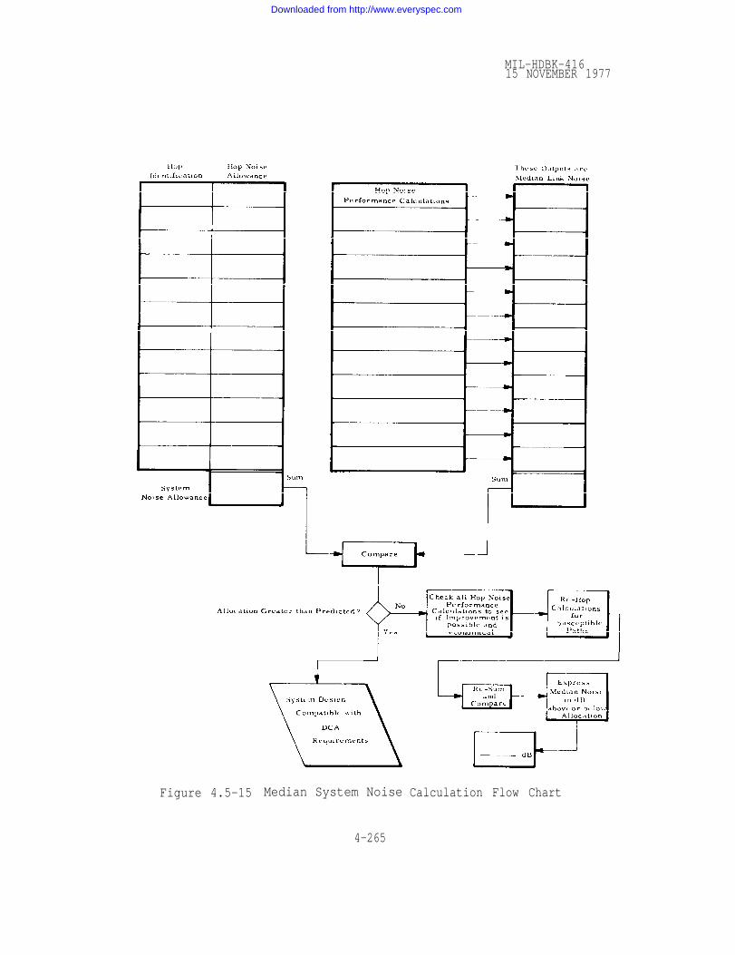
MIL-HDBK-41615 NOVEMBER 1977
Figure 4.5-15 Median System Noise
4-265
Calculation Flow Chart
Downloaded from http://www.everyspec.com

MIL-HDBK-41615 NOVEMBER 1977
Number of equivalent voice
channels, n
4.1
4.2
4.3
4.4
4.5
4.6
4.7
4.8
4.9
4.10
4.11
4.12
4.13
4.14
4.15
4.16
4.17
4.18
sec. 4.1.3
3100 Hz
kHz
(Usable bandwidth)voice channel bandwidth, bc
table 4.5-2(upper basebandlimit)table 4.5-2
maximum modulating
frequency, fm
Baseband bandwidth, BbBb = fm - where kHz
is the lowest frequencyin baseband
step 4.1;par. 4.5.27.2step 4.5
par. 4.5.27.2
step 4.7
par. 4.5.16.4& table 4.5-2
steps 4.6 & 4.9
steps 4.6, 4.8,
-10 + 10 log ndBm0RMS load factor, LF
antilog(LF/20)Numerical RMS load factor
peak factor, PF
Numerical peak factor, pf
RMS per channel deviation,
13.5 dB
4.73
kHz
antilog(PF/20)
RMS carrier deviation, kHz
kHz
kHz
dB
dBm
dBm
4 dB
dB
dB
Peak carrier deviation,
& 4.9
Receiver IF bandwidth, BIF steps 4.3 & 4.11,also table 4.5-2
Receiver noise figure, F par. 4.5.16.4 &4.4.45.13
-174 + 10 log BIF (Hz) + F
-174 + 10 log BIF (Hz)+ F + 10
steps 4.12, 4.13or par. 4.5.27.2
Receiver noise threshold
FM improvement threshold par. 4.5.27.2
sec. 4.5.26
par. 4.5.34.1worksheet 4.4-5step (46)par. 4.5.20.3
for Median Noise Calculations
Pre-emphasis improvement, Ip
Median diversity
improvement, Id
Radio set NPR
Worksheet 4.5-4. Basic Parameters
4-266
-
-
Downloaded from http://www.everyspec.com

MIL-HDBK-41615 NOVEMBER 1977
5.1
5.2
5.3
5.4
5.5
5.6
5.7
5.8
5.9
5.10
5.11
5.12
Transmission line or wave-guide length, transmitter m worksheet 4.4-4
& sec. 4.5.19Type of transmission lineor waveguide
Percent velocity of propa- fig. 4.5-18gation
Velocity of propagation, v m/sec v = (3 x 10⁸) ( x 10-2) par. 4.5.21.4
Echo delay time,
Radian delay
Parameter A
S/D - r
Transmit system
Antenna return loss
RF interface returnloss
Echo amplitude, r
sec
rad
dB
R LANT dB
R LRFI dB
dB
Transmit signal-to-distor-tion ratio, S/D dB
Transmit signal-to-feederecho noise, S/Nf dB
Transmit feeder echo noise, pWO
N f ( t r a n s . )
= 2L/v par. 4.5.21.4
par. 4.5.21.4
A = par. 4.5.21.4
fig. 4.5-19par. 4.5.21.4
par. 4.5.21.5
from applicationstandards ormanufacturer’sspecifications
r = RLANT + RLRFI + 2A par. 4.5.21.5step 5.8, &step (31) fromworksheet 4.4-5
par. 4.5.21.8S/D = (S/D - r) + r steps 5.7 & 5.9
S/Nf = S/D + 10 log -LD par. 4.5.21.8
Nf = antilog par. 4.5.21.8
Worksheet 4.5-5. Transmitter Feeder Echo Noise Calculation
4-267
Downloaded from http://www.everyspec.com

MIL-HDBK-41615 NOVEMBER 1977
6.1
6.2
6.3
6.4
6.5
6.6
6.7
6.8
6.9
6.10
6.11
6.12
Transmission line or wave-guide length, receiver
Type of line or waveguide
Percent velocity ofpropagation
Velocity of propagation, v
Echo delay time, T
Radian delay
Parameter A
S/D - r
Receive system
m
m/sec
sec
rad
dB
Antenna return loss dB
RF interface returnloss dB
Echo amplitude, r dB
Receive signal-to-distortion dBratio, S/D
Receive signal-to-feederecho noise, S/Nf
dB
Receive feeder echo noise,
N f ( r e c e i v e )pWO
worksheet 4.4-4sec. 4.5.19
fig. 4.5-18
v = (3 x 10⁸) ( x 10-2) par. 4.5.21.4
= 2L/v par. 4.5.21.4
par. 4.5.21.4
A = par. 4.5.21.4
fig. 4.5-19par. 4.5.21.4
par. 4.5.21.5
from applicablestandards ormanufacturer’sspecifications
r = RLANT + RLRFI + 2A par. 4.5.21.5step 6.8, &step (32) fromworksheet 4.4-5
S/D = (S/D - r) + r par. 4.5.21.8step 6.7 &6.9
S/Nf = S/D + 10 logpar. 4.5.21.8
= antilog par. 4.5.21.8N f
Worksheet 4.5-6. Receiver Feeder Echo Noise Calculation
4-268
R LA N T
R LR F I
Downloaded from http://www.everyspec.com
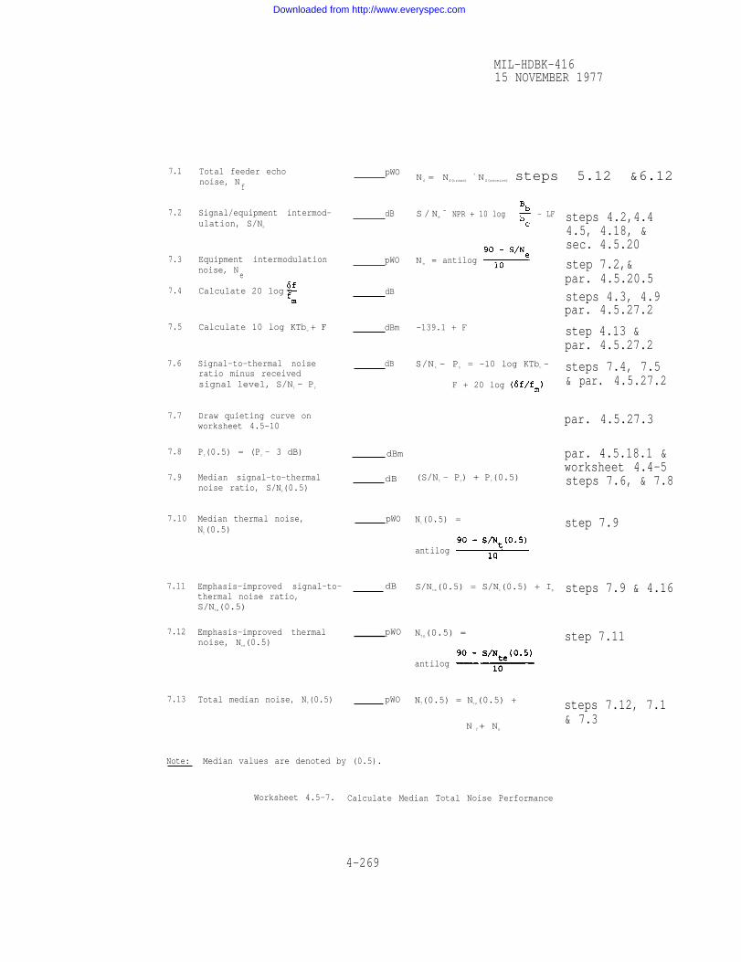
MIL-HDBK-41615 NOVEMBER 1977
7.1
7.2
7.3
7.4
7.5
7.6
7.7
7.8
7.9
7.10
7.11
7.12
7.13
Total feeder echonoise, N
f
Signal/equipment intermod-ulation, S/Ne
Equipment intermodulationnoise, N
e
Calculate 20 log
Calculate 10 log KTbc + F
Signal-to-thermal noiseratio minus receivedsignal level, S/Nt - Pr
Draw quieting curve onworksheet 4.5-10
Pr(0.5) = (Pr - 3 dB)
Median signal-to-thermalnoise ratio, S/Nt(0.5)
Median thermal noise,Nt(0.5)
Emphasis-improved signal-to-thermal noise ratio,S/Nte(0.5)
Emphasis-improved thermalnoise, Nte(0.5)
Total median noise, NT(0.5)
pWO
dB
pWO
dB
dBm
dB
N f = Nf(trans)
+ N f(receive) steps 5.12 &6.12
S / Ne
= NPR + 10 log - LF
N e = antilog
-139.1 + F
S/N t - Pr = -10 log KTbc -
F + 20 log
(S/Nt - Pr) + Pr(0.5)
Nt(0.5) =
antilog
S/Nte(0.5) = S/Nt(0.5) + Ip
Nte(0.5) =
antilog
NT(0.5) = Nte(0.5) +
N f+ Ne
Note: Median values are denoted by (0.5).
Worksheet 4.5-7. Calculate Median Total Noise Performance
4-269
steps 4.2,4.44.5, 4.18, &sec. 4.5.20
step 7.2,&par. 4.5.20.5steps 4.3, 4.9par. 4.5.27.2
step 4.13 &par. 4.5.27.2
steps 7.4, 7.5& par. 4.5.27.2
par. 4.5.27.3
par. 4.5.18.1 &worksheet 4.4-5steps 7.6, & 7.8
step 7.9
steps 7.9 & 4.16
step 7.11
steps 7.12, 7.1& 7.3
dBm
dB
pWO
dB
pWO
pWO
Downloaded from http://www.everyspec.com
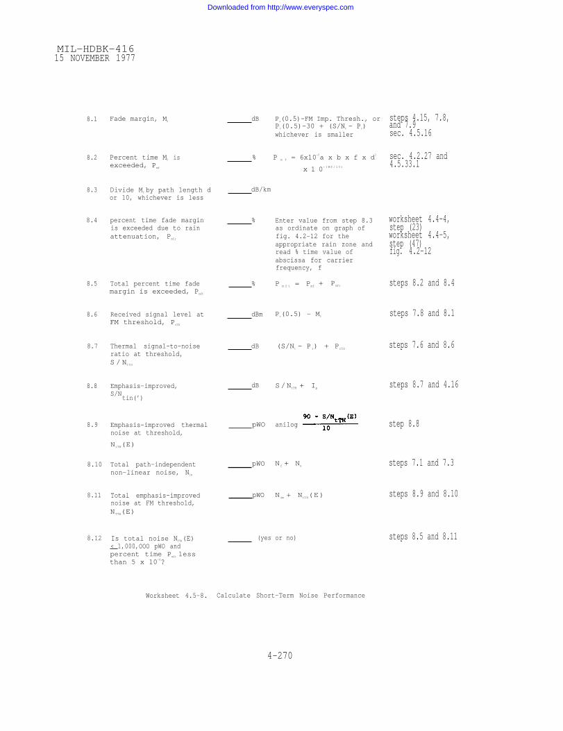
MIL-HDBK-41615 NOVEMBER 1977
8.1 Fade margin, Mf
8.2
8.3
8.4
8.5
8.6
8.7
8.8
8.9
8.10
8.11
8.12
Percent time Mf
exceeded, Pmf
is
Divide Mf by path length dor 10, whichever is less
percent time fade marginis exceeded due to rainattenuation, Pmfr
Total percent time fademargin is exceeded, Pmft
Received signal level atFM threshold, PrTH
Thermal signal-to-noiseratio at threshold,S / NtTH
Emphasis-improved,S/N
tin(’)
Emphasis-improved thermalnoise at threshold,
NtTH(E)
Total path-independentnon-linear noise, Nim
Total emphasis-improvednoise at FM threshold,NTTH(E)
Is total noise NTTH(E)< 1,000,OOO pWO andpercent time Pmft less
dB Pr(0.5)-FM Imp. Thresh., orPr(0.5)-30 + (S/Nt - Pr)whichever is smaller
% P m f = 6x10⁻⁵a x b x f x d3
x 1 0- ( M f / 1 0 )
dB/km
%
%
dBm
dB
dB
Enter value from step 8.3as ordinate on graph offig. 4.2-12 for theappropriate rain zone andread % time value ofabscissa for carrierfrequency, f
P m f t = Pmf+ Pmfr
Pr(0.5) - Mf
(S/Nt - P r) + PrTH
S / NtTH + Ip
anilog
N f + Ne
N im + NtTH(E)
(yes or no)
steps 4.15, 7.8,and 7.9sec. 4.5.16
sec. 4.2.27 and4.5.33.1
worksheet 4.4-4,step (23)worksheet 4.4-5,step (47)fig. 4.2-12
steps 8.2 and 8.4
steps 7.8 and 8.1
steps 7.6 and 8.6
steps 8.7 and 4.16
step 8.8
steps 7.1 and 7.3
steps 8.9 and 8.10
steps 8.5 and 8.11
Worksheet 4.5-8. Calculate Short-Term Noise Performance
4-270
than 5 x 10⁻⁴?
pWO
pWO
pWO
Downloaded from http://www.everyspec.com

MIL-HDBK-41615 NOVEMBER 1977
8.13
8.14
8.15
8.16
8.17
8.18
8.19
8.20
8.21
8.22
8.23
8.24
If “yes”, and diversity was not selected previously, link design iS completed.If “no”, or diversity has already been selected, continue.If “no”, and diversity was not selected previously, re-dosteps 4.17, 4.18, and 7.2 through 8.12; then continue.
Plot line for non-diversityfade margin versus % oftime on worksheet 4.5-11
Read diversity improvement atpercentage Pmft and otherdesired percentage values fortype of combiner used I d ( %)
par. 4.5.34.1steps 8.1 &8.5
fig. 4.5-21worksheet 4.4-4step (46); step 8.5
Decrease fade margin values at
P m f tand other desired per-
centage values by the appropri-ate Id values dB
Plot line for diversity-improvedfade margin versus % of time onworksheet 4.5-11
Diversity and emphasis improvedthermal signal-to-noise ratioS/Nt(E,D) at Pmft percent. dBage of time
Diversity and emphasis improvedthermal noise Nt(E,D) at Pmft
percentage of time
Estimated total percent ofoutage time after diversityand emphasis improvement
Total noise NT(E,D) at Pmft
percentage of time
Is total noise < 1,000,000pWO
Is total outage time5 x 10-4%
If total noise cannot bereduced to < 1,000,000 pWO,estimate percentage oftime during which1,000,000 pWO is exceeded
Mf - Id( %)
S/N tTH + Ip + Id( %) steps 8.8 & 8.15
step 8.18ant i log
Read abscissa for diversity-improved fade margin line onworksheet 4.5-11 where itintersects the ordinatevalue for M
f
Nt(E,D) + Nim
(yes or no) If answers are no,adjust parametersand recalculatenoise performance
(yes or no)
Calculate ratio of totalnoise to 1,000,000 pWO,converted to dB, subtractfrom Mf, and read on the
% diversity improved line ofworksheet 4.5-11 the per-centage value correspond-ing to this ordinate
step 8.16par. 4.5.34.1
steps 8.10 &8.19
step 8.1worksheet 4.5-11
Worksheet 4.5-8. Calculate Short-Term Noise Performance (continued)
4-271
steps 8.1 & 8.17
pWO
%
pWO
Downloaded from http://www.everyspec.com
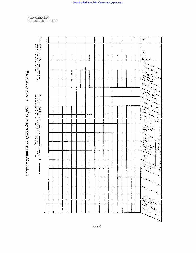
Worksheet 4.5-9
MIL-HDBK-41615 NOVEMBER 1977
4-272
Downloaded from http://www.everyspec.com

Worksheeet 4.5-10.
MIL-HDBK-41615 NOVEMBER 1977
4-273
Downloaded from http://www.everyspec.com

Worksheet 4.5-11.
MIL-HDBK-41615 NOVEMBER 1977
4-274
Downloaded from http://www.everyspec.com

MIL-HDBK-41615 NOVEMBER 1977
4.5.18 Path loss distribution
4.5.18.1 The second major input to the calculations is an
estimated distribution of transmission loss for each radio
hop in order to estimate short-term noise. The long term
median loss may be estimated to be 3 dB greater than the
sum of the free-space loss and the atmospheric attenuation
( see Section 4.2.22 ). The desired short term reliability
has already been defined as 99.9995% corresponding to ap-
proximately two minutes per hop per year when the voice
channel noise is allowed to exceed 1,000,000 pWO. Noise
values of this magnitude in a voice channel are usually
thermal caused by a marked increase in transmission loss.
( We will not consider at this time severe equipment prob-
lems or the even more unlikely occurrence of strong RF
interference. )
4.5.18.2 The likelihood of such thermal noise bursts or
noise increases in a voice channel are related also to the
available fade margin for each radio hop.
4.5.18.3 Fade margin as used here is defined as the decibel
difference in power levels between the normal unfaded signal
( which corresponds to the long-term median loss; see paragraph
4.5.18.1 ) and either the FM threshold level or that received
signal level where the thermal noise equals 106 pWO which-
ever will give the smaller fade margin. For these calcula-
tions, other noise contributions can usually be
4-275
Downloaded from http://www.everyspec.com

MIL-HDBK-41615 NOVEMBER 1977
neglected. To illustrate, consider figures 4.5-16 and 4.5-17. On
figure 4.5- 16, note that for a voice channel capacity of 120 or greater,
the thermal noise exceeds 106 pWO at FM threshold so the fade margin
is the difference in Pr (in dB) between the median value of Pr and that
value of Pr where the channel capacity thermal noise curve crosses the
106 pWO noise level. Thus, for the 600-channel system with 140 kHz
RMS per-channel deviation (on figure 4.5-16) with a median Pr of
-27.5 dBm, the 600 channel curve intersects the 106-pWO level at
Pr = -73.5 dBm. This results in a fade margin of 46.0 dB.
For a per-channel RMS frequency deviation of 200 kHz (as
shown in figure 4.5-17), the thermal noise level of 106 pWO intersects
the 600-channel curve at -76.5 dBm which results in a fade margin of
49.0 dB for the same median value of Pr. Thus the fade margin can
be increased by increasing the per-channel deviation. The fade margin
decreases with increased channel capacity.
4.5.18.4 So far we have discussed fade margin and its calculation for
the individual radio hops in the system. The fade margin required for
each hop to maintain desired link reliability and ways to achieve the
increased margin which may be necessary on difficult links will be dis-
cussed in section 4.5.33.
4.5.19 Select antenna size, transmission line, transmitter power,and calculate long-term median receiver input power
4.5.19.1 At this point, we are ready to begin the calculations required
for the link design summary on worksheet 4.4-4. Items 1 through 16
are now known and the appropriate entries have been made. Items 23,
25, and 26 are also known so a tentative selection of transmission line or wave-
guide type (items 27 and 28) can be made which leads to the values for waveguide
l0SS per unit length (items 29 and 30), and to total waveguide losses
4-276
Downloaded from http://www.everyspec.com
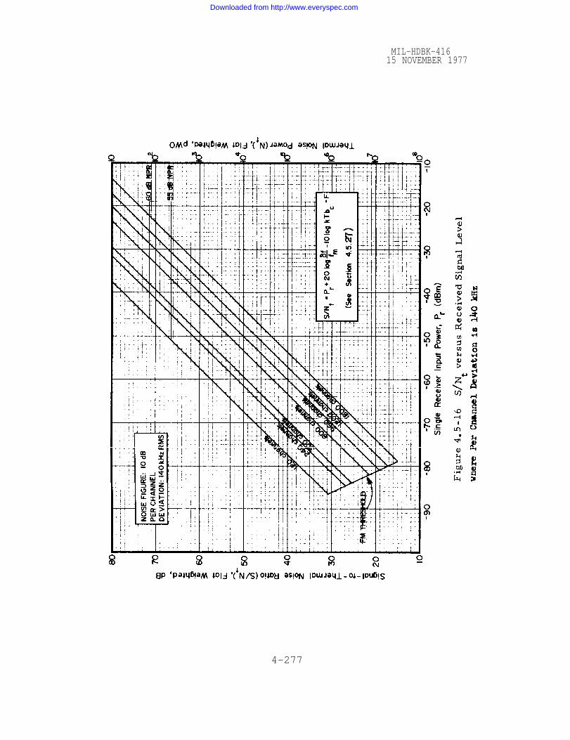
Figure 4.5-16
MIL-HDBK-41615 NOVEMBER 1977
4-277
Downloaded from http://www.everyspec.com
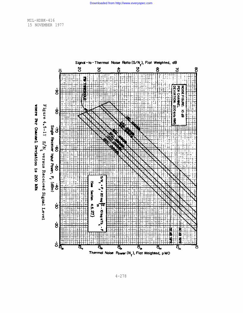
Figure 4.5-17
MIL-HDBK-41615 NOVEMBER 1977
4-278
Downloaded from http://www.everyspec.com

(items 31 and 32). Typical values should
losses (items 33 and 34) and the net fixed
However, these values (items 27 through
MIL-HDBK-41615 NOVEMBER 1977
now be chosen for circulator
losses (item 35) calculated.
35) are tentative estimates
which may be changed as radio hop requirements dictate.
4.5.19.2 The next step is the calculation of free-space basic transmis-
sion loss (item 38) using item 37, path length (from the path profile)
and item 23, carrier frequency. Item 39, the average atmospheric
absorption, is obtained from Section 4.2.22. Since the expected
median receiver input power was initially assumed to be -27.5 dBm, it
can be used in conjunction with the net loss (item 40) to yield the total
gain required to produce this desired received signal level value over
the path. As a first estimate, a transmitter power of +30 dBm (1 watt)
can be used for item 36; this value subtracted from the sum of items
40 and 42 will be the sum of the required antenna gains (items 21 and
22).
4.5.19.3 Consider one of the hops from the example system, in order
to illustrate quantitative results. Hop H between sites 8 and 9 (figure
4.5-11) is 43 kilometers long, will operate with space diversity and
will transmit from site 9 at 8.250 GHz and from site 8 at 8.150 GHz.
Forty-meter towers are assumed necessary at each site, which means
that about 48 meters of waveguide will be required per site. Consider
elliptical waveguide, EW71, which has 6.3 dB loss per 100 meters
and 0.5 dB transmit and 1 dB receive circulator and filter losses.
This results in 7.5 dB for item 35 (worksheet 4.4-5), net fixed losses.
Since transmitter power is expensive, assume initially one watt or
+30 dBm. For the average frequency of 8.2 GHz and a path length of
43 km a free-space basic transmission l0SS value of 143.3 dB is
obtained. From paragraph 4.2.22.2 the atmospheric absorption is
found to be 0.4 dB. Item 40, the net loss is 154.3 dB and if we
4-279
Downloaded from http://www.everyspec.com

MIL-HDBK-41615 NOVEMBER 1977
subtract the difference between +30 dBm for transmitter power and
-27.5 dBm for median received signal level, the required antenna gain
is 96.8 dB. This implies an antenna diameter of 13.5 ft for equal
antennas at both sites (from figure 4.4-30).
4.5.19.4 At this point we must consider recommended limits on anten-
na size given in figure 4.4-33. The maximum diameter for 0.5° half-
power beamwidth is about 16 ft and the recommended diameter is 10 ft.
Although 15-ft dishes can meet the median signal requirements, alter-
native ways to reduce system loss should be explored in order to avoid
extremely narrow antenna beams (see discussion in Section 4.4.29).
As an example 12-ft dishes with 47.2 dB gain and RF preamplifiers at
the receiving antennas could be used. This would reduce the line loss
by 3 dB and maintain the desired median signal level. The use of RF
preamplifiers was discussed in paragraph 4.4.45.12 and illustrated in
figure 4.5-2. It also has the advantage that the receiver noise figure
is reduced which further increases the fade margin.
4.5.20 Equipment intermodulation noise calculation
4.5.20.1 A message passing through a microwave radio relay system
is present in either of two basic forms: as an amplitude -modulated or
frequency-modulated signal. The signal is normally transmitted from
one station to anot her in frequency-modulated form, demodulated and
processed in amplitude-modulated form and re-transmitted in frequency-
modulated form. The presence of modulation in either form causes
instantaneous nonsinusoidal changes in either voltage or frequency
within microwave circuits. Because such circuits cannot be made
completely linear, and cannot respond instantaneously to such changes
in voltage or frequency, spurious signals are produced by each channel
in the system and occur across a wide frequency range. Although the
spurious signals produced in each channel are very small, the additive
4-280
Downloaded from http://www.everyspec.com

MIL-HDBK-41615 NOVEMBER 1977
effect from a large number of signals in several channels beating to-
gether forms intermodulation noise signals whose amplitude is large
enough to impair the performance of communications links. Some of
these spurious signals will fall within the bandwidth of adjacent chan-
nels, causing inter modulation noise to appear there. The magnitude
of the intermodulation noise is a function of equipment characteristics,
the number of channels in the system, and the modulation levels in the
channels producing the noise. The higher the modulation level in the
channels producing the spurious signals, the higher the intermodulation
noise will be in those adjacent channels whose bandwidths coincide with
the frequencies of these noise products. The values of the inter-
modulation noise under specific channel loading conditions must be
obtained from equipment performance specifications, or the intermodu-
lation noise must be measured under actual operating conditions.
4.5.20.2 Intermodulation noise, for the purpose of system noise cal-
culations, is defined as the total noise from all sources produced as a
result of the presence of a modulated signal in the system. Intermodu-
lation noise is measured in a channel with all modulation removed from
the channel being measured, and with all remaining channels loaded
with actual traffic or with an equivalent amount of white (randomly-
distributed) noise over a specific bandwidth. The intermodulation
noise power in the channel is then equal to the measured total noise
with modulation present less the measured thermal noise with no
modulation present.
4.5.20.3 A common method of determining total noise under maximum
traffic conditions consists of using a “white noise” generator which
produces a noise spectrum approximating that produced in a multi-
channel multiplex system. The output noise level from the generator
is adjusted to a desired multiplex composite baseband level (composite
4-281
Downloaded from http://www.everyspec.com

MIL-HDBK-41615 NOVEMBER 1977
noise power). Then, a notched filter is switched in to clear a narrow
slot in the spectrum of the noise signal, and a noise analyzer is con-
nected at the output of the system. The analyzer can be used to measure
the ratio of composite noise power to the noise power in the cleared
slot, which is equivalent to the total noise (thermal plus intermodula-
tion) present in the slot bandwidth. Usually, the slot bandwidth is
made equal to the bandwidth of a single multiplex channel; thus the
noise power in the slot is the same as the total noise in a typical multi-
plex channel. Usually, measurements are made at the upper, lower
and center frequencies of the baseband. The ratio of the composite
noise power in the baseband to the total noise power in the slot is
usually called the noise power ratio. (NPR). When this NPR measure-
ment is made at high RF levels, corresponding to the median received
in a back-to-back configuration, the dominant component of noise is
that due to equipment intermodulation. This parameter is used as an
approximation of the equipment intermodulation noise contribution, and
should be obtained from operations and maintenance records or from
published manufacturers’ specifications on the equipment to be used
including the stated equivalent noise loading. If information is not
available, an NPR value of 55 dB obtainable using new, quality equip-
ment is probably the highest value that can be assumed for the initialestimate. However, some methods of diversity combining can also improve
the NPR. As an example, for equal gain or maximal ratio combining thesignal powers are added coherently while intermodulation noise contributions-
similar to other types of noise- are added randomly. This justifies a 3 dB
improvement in NPR valuesassumed for the examples discussed here (section
4.5.16 and worksheets of section 4.5.41).
4.5.20.4 The above discussions hold for demodulating (baseband)
radios. If the designer is concerned with heterodyne repeaters, the
above measurements become very difficult to make, and the designer
has to rely on manufacturers specifications. Alternatively, a 4 dB
improvement in NPR [14] over the demodulating radio may be assumed.
For example, if a 55 dB NPR is assumed for the demodulating radio,
a 59 dB NPR would be used for a similar heterodyne unit.4-282
Downloaded from http://www.everyspec.com

MIL-HDBK-41615 NOVEMBER 1977
4.5.20.5 The noise power ratio can now be converted to an equivalent
noise channel signal-to-equipment inter modulation noise ratio, S/Ne,
and additionally to equipment intermodulation noise, Ne. This is
expressed, in dB, as:
S/Ne = NPR + 10 log (Bb/bc-LF)dB
Ne = antilog pWO*
(4.5-1)
(4.5-2)
where Bb is the baseband width,
bc is the nominal voice channel bandwidth, 3100 Hz, and
LF is the RMS load factor in dB (see Section 4.5.27).
Bb and bc must be in the same units.
4.5.20.6 Allocation of calculated noise is difficult particularly for
mixed systems on a hop; i.e., a demodulating transmitter at one end
and a heterodyne repeater receiver at the other end. Very little infor-
mation exists on the noise contribution of the individual components or
even that of the transmitter and receiver separately. For an engineer-
ing estimate, the equipment intermodulation noise may be allocated in
equal parts to the transmitter side and the receiver side.
4.5.20.7 The foregoing calculations are for the top voice channel of
the system which is normally assumed to be the “worst” channel in
terms of noise and performance.
4.5.20.8 Equipment intermodulation noise is considered to be inde-
pendent of path loss or received signal level variations. Consequently,
it will be considered as a component of the time invariant nonlinear
noise (figure 4.5-14).
*It should be noted that in the noise calculations of these sections flat-weighted noise will be used for ease in handling. If the designer de-sires to use other noise weighings, appropriate factors may be in-cluded at the conclusion of the design procedure.
4-283
Downloaded from http://www.everyspec.com

15 NOVEMBER 1977
4.5.21 Feeder intermodulation noise calculation
4.5.21.1 If a transmission line many wavelengths long is mismatched
at both the generator and load ends, its frequency-phase response is
linear with a small sinusoidal ripple, and this leads to reflected waves
in the line that cause distortion of an FM signal. This type of distor-
tion is more conveniently considered as being caused by an echo signal
generated in a mismatched line, which results in inter modulation
distortion. Significant levels of this type of intermodulation noise are
reached when the waveguide lengths exceed approximately 20 meters
per individual antenna, or 30 meters total per hop.
4.5.21.2 The feeder intermodulation noise is also considered to be
independent of path loss or signal level variations and is therefore
another component of the time invariant non-linear noise power.
4.5.21.3 Calculations of feeder intermodulation noise is well treated
in the literature [13], [80]. It may be approximated given transmis-
sion line lengths (worksheets 4.5-5 and 4.5-6), velocity of propagation
in the lines, transmission system component VSWR’s and directional
losses. The calculations are performed separately for each end of a
hop; i. e., transmitter and receiver, and the results are summed to
determine the total hop contribution. Procedures are as follows:
4.5.21.4 Determine echo delay time, from the transmission line
length, L, and the percent velocity of propagation, (% v),
obtained from figure 4.5-18, using:
=
2L/V sec, where V=(3x10⁸)(%vx10-2)m/sec.
The echo delay time is then converted to radian delay:
Radian delay =
(4.5-3)
(4.5.-4)
4-284
MIL-HDBK-416
Downloaded from http://www.everyspec.com

MIL-HDBK-41615 NOVEMBER 1977
Courtesy of Dr. John Osepchuk and Horizon House, Inc.
Figure 4.5-18 Waveguide Velocity Curves
4-285
Downloaded from http://www.everyspec.com
MIL-HDBK-41615 NOVEMBER 1977
where fmis the highest modulating frequency in the baseband.
Next a " parameter A " is determined from the following
equation:
A = ( 4.5-5 )
where is the composite RMS carrier deviation ( is the
product of ) and fm as defined earlier. The symbol
is the numerical load factor, antilog LF/20. Using the par-
ameters A and the radian delay, a value for signal-to-distortion
ratio minus echo amplitude, ( S/D - r ), may be determined from
the curves in figure 4.5-19.
4.5.21.5 It now remains to determine the echo attenuation, r.
Consider the top illustration in figure 4.5-19a. The echo energy
at the transmitter side travels along the path shown, and is reduced
by each reflection at an interface by the return loss associated
with the voltage standing wave radio ( VSWR ) at that interface.
Such values of return loss ( or VSWR ) must be measured with
the equipment in its operating configuration. Return loss values
for the radio frequency interface, the antenna input, and the trans-
mission line ( measured at the point where it connects to the RF
interface with the antenna connected ) my be assumed to be at least
26 dB corresponding to a VSWR value of 1 : 1.10. However,
return loss values of 32 dB or better corresponding to VSWR values
of 1 : 1.05 are not unrealistic, and are frequently specified. The
relations between return loss, reflection coefficient, and standing
wave ratio are given in the next paragraph.
4.5.21.6 The echo energy is reduced by the return loss at the
4-286
Downloaded from http://www.everyspec.com

MIL-HDBK-41615 NOVEMBER 1977
Figure 4.5-19 Maximum Distortion to Signal Ratio due to Echo
4-287
Downloaded from http://www.everyspec.com
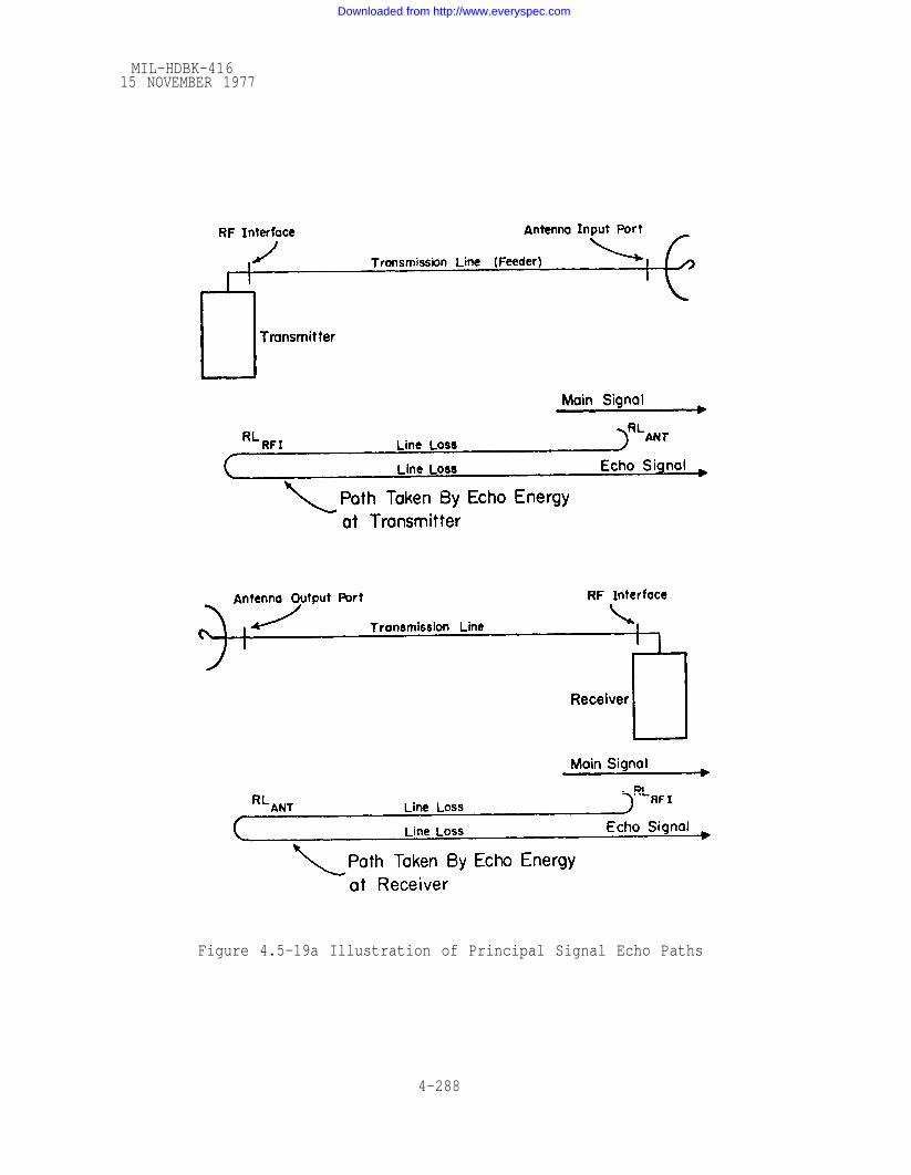
MIL-HDBK-41615 NOVEMBER 1977
Figure 4.5-19a Illustration of Principal Signal Echo Paths
4-288
Downloaded from http://www.everyspec.com

MIL-HDBK-41615 NOVEMBER 1977
antenna port, the one -way attenuation through the transmission
line antenna feeder, the return loss at the RF interface, and
another one-way attenuation through the same line. The total
echo attenuation in dB is thus the sum of these decibel losses.
Similar considerations apply to the echo attenuation at the re-
ceiver side as shown in the lower portion of figure 4.5-19a.
If parameters other than return loss are provided such as the
VSWR or the voltage reflection coefficient,
verted to return loss, RL, using the following
they can be con-
expressions:
( 4. 5-6 )
( 4.5-7 )
Also, table 4.5-3 or figure 4.5-20 can be used for this conversion.
4.5.21.7 The approach described above is somewhat conservative,
and may slightly overestimate voice channel feeder echo noise since
it assumes that the reflections of the echo energy will result in max-
imum delay time and hence in nearly maximum noise. This occurs
because the echo energy arriving at the RF interface in the case of
the transmitter ( or the antenna in the case of the receiver ) in fact
contains components that have been reflected at many intermediate
points along the transmission line ( such as waveguide joints or
transitions ). All of these have shorter delay times than the total
echo path.
4.5.21.8 The calculation of echo attenuation ( separately for trans-
mitter and receiver ) outlined above can now be converted to voice
channel noise. To do this, the total echo attenuation, r, is added
to the ( S/D - r ) value obtained from the procedures in paragraph
4.5.21.4. This results in the signal-to-distortion ratio, S/D which
4-289
Downloaded from http://www.everyspec.com
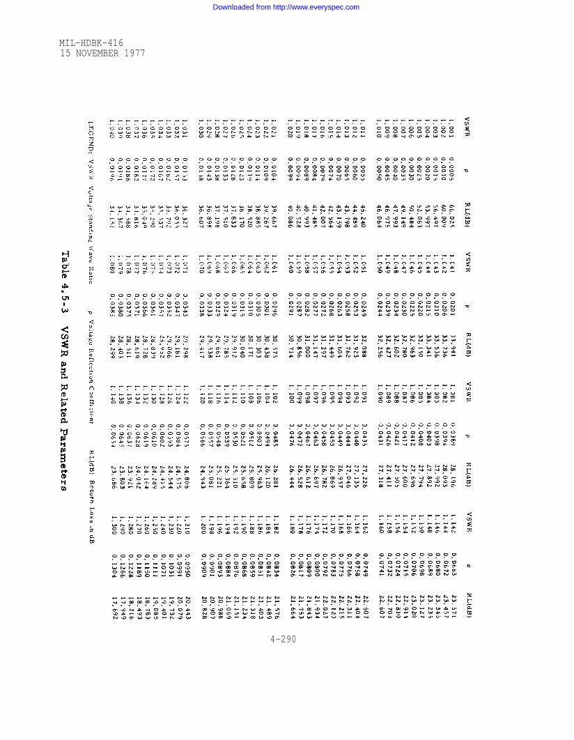
Table 4.5-3
MIL-HDBK-41615 NOVEMBER 1977
4-290
Downloaded from http://www.everyspec.com

MIL-HDBK-41615 NOVEMBER 1977
4-291
Downloaded from http://www.everyspec.com
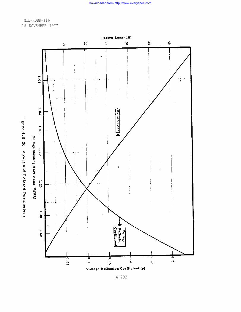
Figure 4.5-20 4-292
MIL-HDBK-41615 NOVEMBER 1977
Downloaded from http://www.everyspec.com

MIL-HDBK-41615 NOVEMBER 1977
must be corrected for the ratio of baseband to voice channel
bandwidth and for the RMS load factor. In equation form, the
voice channel signal to feeder echo noise ratio becomes:Bb
S/Nf = S/D + log----- - LF dB (4.5-8)
The conversion to flat-weighted noise is as follows:90-S/Nf
Nf = antilog pWO.10
The foregoing feeder echo noise calculations are performed
separately for each end of a hop by arbitrarily designating one
end the transmitter and the other end the receiver. At the con-
clusion, these two noise results are summed together to give a
total hop feeder echo noise contribution.
4.5.22 Time-invariant nonlinear noise
4.5.22.1 The sum of the total feeder echo noise and equipment
intermodulation noise in this design will be called the time in-
variant nonlinear noise since these noise components do not depend
on path loss variability. This total noise component is normally
the dominant contribution for relatively high signal levels near the
long -term median. For this case, an approximation may be made in
the long -term noise calculations by omitting the smaller thermal
noise contribution which will be discussed in the following paragraph.
Conversely, the time-invariant nonlinear noise may be dropped for
approximating short-term noise calculation at low signal levels near
FM threshold since the thermal noise contribution will now be the
dominant factor.
4.5.23 Thermal noise
4.5.23.1 As a natural law, thermal noise is always present. Its
power depends on the absolute temperature of the point where it is
4-293
Downloaded from http://www.everyspec.com
MIL-HDBK-41615 NOVEMBER 1977
measured, and also on the bandwidth. The thermal noise power per Hz
bandwidth at the radio-relay receiver input is given by the expression
At an ambient temperature of 27° C (300° K) this is 4 x 10-21
kTo. W/Hz
which corresponds to a power level of -174 dBm/ Hz. It can be seen
directly from the expression given, that the thermal noise power of the
point considered can be reduced by cooling this point. Very low tem-
peratures are required to get a remarkable improvement in thermal
noise. This is very expensive and, therefore, not used on terrestrial
radio-relay systems. In addition, the noise power seen by antennas
pointed at low elevation angles is about -174 dBm/Hz making very
little improvement possible by cooling the receiver input impedance.
4.5.23.2 The thermal noise power measured at the receiver output
s hews a higher value than one would expect from the thermal noise of
the input alone. The difference between both these values is the thermal
noise power produced in the receiver itself. By special measures it
can be kept small. But some of these measures are very expensive,
because they are also using the cooling of equipment to very low
temperatures. Normal radio-relay systems must be economical in
use, and for this reason it is unwise to employ expensive methods only
to get a few dB of improvement.
4.5.23.3 The thermal noise characteristics of the receiver which add
to the input thermal noise are expressed by the “receiver noise figure”
in dB which is the ratio of the thermal noise measured at the receiver
output to the thermal noise expected at the same point if only the am-
bient noise given by kTois present at the receiver input. Because of
the reasons mentioned above, most practical microwave systems have
receiver noise figures of about 10 dB.
4.5.23.4 In the frequency bands of interest here the thermal noise
power per Hz bandwidth is constant. The total thermal noise power
4-294
Downloaded from http://www.everyspec.com

MIL-HDBK-41615 NOVEMBER 1977
of a receiver is therefore directly proportional to the bandwidth of the
receiver.
4.5.23.5 Thermal noise has random characteristics with substantial
fluctuations relative to its mean power so that even very high peaks
can occur with a small probability.
4.5.24 Points at which thermal noise power can influence the signal
4.5.24.1 It has already been mentioned that the thermal noise can
influence the useful signal at the receiver input where the useful signal
is at a very low level. But also within the receiver there are several
points with low signal levels where thermal noise is added and can
therefore contribute to the total
the inputs of amplifiers. These
amount of thermal noise in well
thermal noise of the receiver such as
points do not contribute a significant
designed systems.
4.5.25 The mechanism by which the thermal noise power caninfluence the signal
4.5.25.1 Thermal noise signal can be assumed to be voltage vector
with varying amplitude and phase which is added to the useful signal
represented by a frequency modulated carrier of constant amplitude.
The vector resulting from the addition of the noise vector and the
carrier vector is then a vector with both amplitude and phase varying.
Within the
amplitude
4.5.26
4.5.26.1
receiver this signal passes an amplitude limiter so that its
is made constant again, but its phase is still disturbed.
Pre-emphasis
After demodulation, thermal noise power increases with
baseband frequency so that the higher channels have smaller signal-to-
thermal-noise ratios than the lower ones. To compensate for this
effect in most radio-relay systems, pre-emphasis is applied. This
means that before frequency modulation is accomplished in the
4-295
Downloaded from http://www.everyspec.com

MIL-HDBK-41615 NOVEMBER 1977
transmitter the level of the
while the level of the lower
ner so that the mean power
pre-emphasis. Therefore,
upper part of the baseband is increased
part is decreased. This is done in a man-
in the baseband is the same with or without
the C. C. I. R. in its Recommendation 275
[81] has standardized frequency characteristic of pre-emphasis for
all types of broadband systems. Between the lowest and the highest
telephone channel this pre-emphasis value is 8 dB, and the mean pre-emphasis
improvement Ip =4dB.4.5.27 Calculate long-term median thermal noise
4.5.27.1 For purposes of system noise calculations, thermal noise
is defined as noise from all sources in a channel when there is no
modulated signal present on any of the channels in the microwave
system. By this definition, thermal noise includes atmospheric and
cosmic noise, and all intrinsic and thermal noise produced in the
equipment when no modulation is present. Thermal noise is measured
in a channel with all modulation removed from all channels of the
systerm.
4.5.27.2 The signal-to-thermal noise ratio in an FDM-FM system is
related to path loss variability. As the path loss on a hop becomes
low; i. e. , the received signal level becomes high, the thermal noise
is quite low and as received signal level decreases toward FM thres-
hold, the thermal noise becomes proportionally higher. Signal-to-
thermal noise ratio, S/Nt, in a voice channel is proportional tO received
signal level Pr or carrier-to-noise ratio C/N in the region above FM
threshold (usually taken as 10 db above thermal noise threshold). It may
be expressed in several forms for this region, as follows:
S/Nt
= P +20 log — -10 log kTbc - Fr f m
(4.5-l0)
S/Nt
= P +20 log -PF - LF - 10 log kTb - F (4.5-11)r c
4-296
Downloaded from http://www.everyspec.com

MIL-HDBK-41615 NOVEMBER 1977
and LF = -10 + 10 log n in dB
(4.5-12)
(4.5-13)
(4.5-14)
(4.5-15)
F is the peak carrier deviation in kHz
is the rms per channel deviation in kHz
S/Nt is the voice channel signal to thermal noise ratio in dB
P is the received carrier level in dBm,r
C/N is the predetection carrier-to-noise ratio in dB and Nis the receiver front end thermal noise power in thesame units as P
rPF is the baseband signal peak factor of 13.5 dB
LF is the RMS noise load factor in dB
bc is the useable voice channel bandwidth taken to be 3.100in kHz
BIF
is the receiver IF bandwidth in kHz
fm is the highest modulating frequency in the baseband inkHz
F is the receiver noise figure in dB
k is Boltzman’s constant, 1.3804 x 10 -20millijoules/ 0K,and
T is the antenna temperature taken to be 290°K.
n is the number of voice channels in the baseband.
4.5.27.3 The terms on the right hand side of the first two equations
with the exception of P may be calculated for a given set of equipmentr
parameters. This then becomes a constant - a figure of merit - and as
P is allowed to vary the vo0ice channel signal-to-thermal-noise ratior
4-297
Downloaded from http://www.everyspec.com

MIL-HDBK-41615 NOVEMBER 1977
varies in proportion. Using this information, a receiver transfer character-
istic or “quieting curve” similar to those in figures 4.5-16 and 4.5-17 may be
constructed, where its slope is uniquely determined by any of the above
equations for conditions above FM threshold.
4.5.27.4 The quieting curve is a good indication of the link dynamic per-
formance characteristics. It is essentially a plot of voice channel signal-to-
noise ratio versus received signal level. For a graph that is linear in decibels
such as worksheet 4.5-10, the main portion of the quieting curve is a straight
line with unity slope in accordance with the equations in paragraph 4.5.27.2.
This portion is limited at the upper end (high received signal
equipment intermodulation noise, and at the lower end by the
threshold where the linear relationships of equations (4.5-10,
-13 ) no longer hold.
levels) by the
FM improvement
-11, -12, and
4.5.27.5 A good approximation to the quieting curve can be constructed in
the following manner on worksheet 4.5-10 using information from the preceding
worksheets:
a. Determine received signal level for which the signal-to-thermal
noise ratio equals zero (from step 7.6 on worksheet 4.5-7), increase this value
by 20 dB, and plot this point on the graph at the 20 dB ordinate value.
b. Draw a straight line with unity slope through this point.
c. Mark on this line the point corresponding to the FM improvement
threshold (step 4.15 on worksheet 4.5-4) as abscissa value.
d. Draw a horizontal line at the ordinate corresponding to the signal-
to-equipment intermodulation noise ratio S/Ne (from step 7.2 on worksheet 4.5-7).
e. The available dynamic range for linear system performance is that
portion of the unity - slope straight line between the FM improvement threshold
and the line intersection with the S/Ne line from (d.) above.
f. Performance below the FM improvement threshold can be approx-
imated by a line with a slope of 4 (4 dB decrease in signal-to-noise ratio for
each 1 dB decrease in received signal level) at S/N values lower than that
corresponding to the FM improvement threshold.
4-298
Downloaded from http://www.everyspec.com

MIL-HDBK-41615 NOVEMBER 1977
4.5.27.6 The completed worksheet 4.5-10 in section 4.5.41 provides an
example of a quieting curve. Transitions between the three straight -line
portions of the curve can be made by rounding as shown.
4.5.28 Determine long -term median total noise performance
4.5.28.1 The preceding sections have shown the calculations of all noise
contributions from several sources. The median noise for each hop is the
sum of the thermal noise calculated for the long term median and the time -
invariant equipment and intermodulation noise.
4.5.29 Compare hop predicted noise with noise allowance
4.5.29.1 The next step is to compare the calculated long -term median
total noise with the noise allowance which was determined in Section
4.5.16 and entered on worksheet 4.5-3. The calculated noise should be
compared with the per -hop estimated total noise rather than the allocated
per-hop noise. If the calculated noise is only slightly larger than this esti-
mate, no readjustment should be made at this point unless the estimated
system noise is nearly equal to or greater than the total system allocation.
Other links may be more favorable than the estimate and the link design
may be adequate.
4.5,30 Adjust hop/equipment requirements
4.5.30.1 When a calculation shows that a hop will not meet the median
estimated noise requirement the sources of noise should be checked to
see which one or ones exceed those estimated on worksheet 4.5-3.
4.5.30.2 It becomes at this point a matter of evaluating the cost of
the necessary improvements. For instance, if more transmitter power
is required, the cost of the power amplifier must be balanced against
the requirement, Such decisions may need to be deferred to a higher
authority.
4-299
Downloaded from http://www.everyspec.com

MIL-HDBK-41615 NOVEMBER 1977
4.5.31 Estimate short-term signal levels at the receiver input
4.5.31.1 The purpose of this section is to check the adequacy of the
equipment parameters to meet the short-term time availability require-
ments which correspond to total voice channel noise power less than.
1,000,000 pWO
corresponds to
and requires a
during 99.9995% of the year. This time availability y
an allowable outage time of about 2 minutes per year,
large fade margin. Its magnitude can be estimated
usually from two causes of signal fading, namely rain attenuation and
multipath propagation. These effects were discussed in sections 4.2.24
and 4.2.27 respectively. In general, these two effects will not occur
simultaneously since heavy rain will break up any atmospheric stratifi-
cation responsible for multipath and conversely, during periods of
considerable atmospheric stratification, rains heavy enough to cause
much attenuation are very unlikely.
4.5.32 Rain attenuation
4.5.32.1 Since rain attenuation can not usually be alleviated by
diversity operations, one must evaluate the percentage of time the
radio hop attenuation is likely to cause the voice channel noise to
exceed 1,000,000 pWO.
4.5.32.2 The first step is to determine the applicable rainfall zone
from the maps in Section 4.2.24. To continue with the example of
Hop H, assume that it is in Rainfall Zone 3. From the calculations in
Section 4.5.18 there is a 48.8 dB fade margin available using 600
voice channels with 200 kHz per-channel deviation. In Section 4.5.19
we considered using an RF preamplifier to increase system gain and
reduce the receiver noise figure, in this case from 10 dB to about
6 dB. This will provide a fade margin increase of 4 dB to 52.8 dB.
4.5.32.3 A fade margin of 52.8 dB can be pro-rated to 5.28 dB/km
for a 10 km rain cell diameter (as discussed in Section 4.2.24).
4-300
Downloaded from http://www.everyspec.com
MIL-HDBK-41615 NOVEMBER 1977
For the example, figure 4.2-12b (Rain Zone 3) is used to estimate the
percent of time for which the attenuation over the link will exceed this
value by entering 5.28 dB/km as the ordinate and determining the
corresponding abscissa value for the (approximately) 8.2 GHz carrier
frequency. In this case thie involves visual interpolation between the
curves for 7 and 10 GHz. The result is the percentage of time during
which the 52.8 dB fade margin, pro-rares as described above, will exceede.
For the example, this is less than 0.0001% of the time, or less than
32 seconds per year.
5.4.33 Multipath Fading.
4.5.33.1 Equation 4.2-22 in Section 4.2.27 is used to calculate the
percentage of time that multipath fading will cause voice channel noise
to exceed 106 pWO. Appropriate values of the constants “a” and ”b”
based on the terrain and climate of the radio hop must be selected
which is somewhat arbitrary and a matter of engineering judgement.
For Rain Rate Zone 3 appropriate values might be a = 1 and b= 1/4.
For a 43 km path length and 8.2 GHz carrier frequency, the fade-7
margin is exceeded during a fraction of 5.1 x 10 of the year or
0.000051% outage time.
4.5.33.2 To evaluate the total hop outage per year, the outage times
due to rain attenuation and multipath are summed and the total com-
pared with the desired value of 0.0005%. For the example the total
estimated outage time will be less than 0.000151%. This is an indica-
tion that the link design is adequate.
4.5.33.3 If, for some hop, the estimated total outage time exceeds the
allocated time of 2 minutes per year, fade margin is not sufficient
and will have to be increased if the reliability requirements must be
met. The methods for increasing fade margin, such as improving
noise figures, increasing antenna size and increasing transmitter
power are expensive, but can be evaluated in terms of cost versus
increased reliability. Before such methods are considered, we should
evaluate potential improvement by diversity operation.
4-301
Downloaded from http://www.everyspec.com

MIL-HDBK-41615 NOVEMBER 1977
4.5.34 Diversity
4.5.34.1 If a particular hop will not meet the time availability require-
ment, the advantages of diversity reception may be considered since at least
fading depth due to multipath can be substantially reduced as shown in figure
4.5-21 for dual space diversity. This figure is based on the improvements
shown in [82] out to the point corresponding to 99.99% of the time reliabil-
ity (0.01% outage time). Extension of the curves in figure 4.5-21 are
straight -line extrapolations as a first approximation. The fade depth for
any fraction of the year given by the abscissa will be reduced by the amount
of diversity improvement read on the corresponding ordinate for the appli-
cable type of combiner. Thus, at 0.0005%, a diversity gain of about 26 dB
is expected for selection combining which will reduce the required fade
margin by the same amount. Figure 4.5-22 shows the effect of such an
improvement on the example hop, and worksheet 4.5-11 is provided as an
aid in preparing similar graphs for specific links under study. The rela-
tions between percentages of time and fade margin in dB are approximated
by straight lines in order to facilitate extrapolations beyond the scale pro-
vided. One may select two convenient values of the fade margin, Mf,
calculate the corresponding percentages P mft using the step-by-step
procedures in worksheet 4.5-8, plot the points on worksheet 4.5-11, and
draw a straight line through these points. Useful values of Mf will usually
be between 10 and 20 dB and 30 and 40 dB, respectively; the threshold value
may of course be used for one of the values if it falls within the range of
the graph. For the example discussed here, a fade margin of only 20 dB
would be adequate to provide not more than 0.0001% of the year outage
time if dual diversity is used. Median diversity improvement, Id, as
entered in worksheet 4.5-4, can be estimated from [82] as approximately
2.5 dB for selection, 3.0 dB for equal gain, and 3. 5 dB for maximal ratio
combiners.
4.5.34.2 Questions might arise why such large fade margins are
designed into the hops if much smaller margins would suffice. One reason
4-302
Downloaded from http://www.everyspec.com

Figure 4.5-21
MIL-HDBK-41615 NOVEMBER 1977
4-303
Downloaded from http://www.everyspec.com

Figure 4.5-22
MIL-HDBK-41615 NOVEMBER 1977
4-304
Downloaded from http://www.everyspec.com

MIL-HDBK-41615 NOVEMBER 1977
is that the low median noise requirements usually will provide large fade
margins. Another reason is that occasionally severe power fading will
occur due to ducting or trapping, and diversity will not be effective. How-
ever, if a large fade margin has been designed into the system, there is a
much better chance that the system will not have excessive noise during
severe power fading.
4.5.34.3 Diversity combining techniques such as post-detection maxi-
mal ratio and linear addition may entail some risk for digital transmission
because of unknown and varying differential time-of -arrival values. If the
times of arrival of two like data streams are delayed relative to each other
by more than approximately one quarter of a bit interval (on the order of
nanoseconds for high-speed data), addition on a power or voltage basis may
cause serious pulse distortion and give rise to error bursts. For this
reason, a baseband switch that selects one or the other of the data streams
is preferable although the switching function itself may introduce error
bursts. However, provisions can be made to avoid unnecessary switching.
Instead of letting a set differential in signal level actuate switching regard-
less of the absolute signal level in the two channels, the switch should be
disabled until the signal level of one channel is reduced to values close
to threshold; if then the level of the other channel is significantly higher,
switching may proceed.
4.5.34.4 A further improvement to be made is clock averaging and
bit coherence of the demodulated data stream so that switching will in
essence be error-free. This and similar methods are denoted by the
term “hit-less switching”.
4.5.34.5 Pre-detection diversity combiners for digital systems
require devices to insure coherency of the radio frequency phase ( similar
to those for FDM/FM systems) in order to avoid loss of synchronization
and excessive error bursts. Additionally, modulation coherency is also
required and may be more difficult to achieve.
4-305
Downloaded from http://www.everyspec.com

MIL-HDBK-41615 NOVEMBER 1977
4.5.34.6 At this time there is little information available on the
performance of various combining techniques for high-speed digital data;
an extensive test program would be required to obtain useful quantitative
information that can be applied to system de sign.
4.5.35 Complete system summary charts
4.5.35.1 The next step in the design is to enter the total median noise
calculated for each radio hop on figure 4.5-15 and sum the median noise
values. This is compared with the System Noise Allocation.
If the calculated noise exceeds the allocation, the individual links
should be checked with the idea of reducing median noise. This effort
to reduce the noise will be a matter of the cost and feasibility of modi-
fications as already stated.
4.5.35.2 If some of the hops are changed, a new set of design sheets
should be prepared and labeled "Issue 2" to ensure that the latest
applicable design will be used.
4.5.36 System reliability
4.5.36.1 Mathematical models used to make reliability calculations for
systems and subsystems ignore common causes of system failures
since they are usually based on reliability figures for random failure
of individual components from historical data for similar components
operating with load conditions similar to those expected in the system.
In addition to such component failures, real system failures may also
occur because of human error in design, manufacture, installation,
operation, and maintenance. Although reliability calculations will
usually not accurately predict the reliability of a microwave subsystem,
they are useful because no subsystem is likely to work adequately if the
computations indicate a lack of required reliability. System reliabil-
ity may be estimated in three ways:
a. on the basis of the reliability of its components;
b. on the basis of statistics for similar systems; and
4-306
Downloaded from http://www.everyspec.com
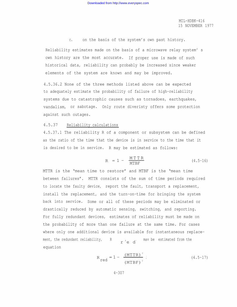
MIL-HDBK-41615 NOVEMBER 1977
c. on the basis of the system’s own past history.
Reliability estimates made on the basis of a microwave relay system’ s
own history are the most accurate. If proper use is made of such
historical data, reliability can probably be increased since weaker
elements of the system are known and may be improved.
4.5.36.2 None of the three methods listed above can be expected
to adequately estimate the probability of failure of high-reliability
systems due to catastrophic causes such as tornadoes, earthquakes,
vandalism, or sabotage. Only route diveristy offers some protection
against such outages.
4.5.37 Reliability calculations
4.5.37.1 The reliability R of a component or subsystem can be defined
as the ratio of the time that the device is in service to the time that it
is desired to be in service. R may be estimated as follows:
R = 1 -M T T RMTBF
(4.5-16)
MTTR is the “mean time to restore” and MTBF is the “mean time
between failures”. MTTR consists of the sum of time periods required
to locate the faulty device, report the fault, transport a replacement,
install the replacement, and the turn-on-time for bringing the system
back into service. Some or all of these periods may be eliminated or
drastically reduced by automatic sensing, switching, and reporting.
For fully redundant devices, estimates of reliability must be made on
the probability of more than one failure at the same time. For cases
where only one additional device is available for instantaneous replace-
ment, the redundant reliability, R , mav be estimated from ther e d-
equation
R = 1 - (MTTR) 2
red(MTBF) 2
.l (4.5-17)
4-307
Downloaded from http://www.everyspec.com

MIL-HDBK-41615 NOVEMBER 1977
4.5.38 A practical example of LOS system reliability
4.5.38.1 Empirical information on the reliability of major long-
distance Canadian radio-relay systems for the period 1963 - 1968
inclusive is given in [81], pp 133 - 138. Figure 4.5-23 shows the
percent reliability based on the 2500 km Canadian system. Note the
reliability increase for successive years. The total interruption time
given by the complement of the ordinate in 4.5-23 divided into its
various components is shown in figure 4.5-24 and the distribution of
the various outage causes noticeable changes as the system ages.
4.5.39 Causes of system outage
4.5.39.1 Listed below are some causes of system outage.
a. Interference from
b. Interference from
c. Signal fading over
d. Equipment failurefailures.
e. Equipment failure
f. Equipment failure
external sources.
internal system sources.
individual hops.
due to component or subsystem
due to human error.
due to catastrophic events suchas tornados and earthquakes.
g. Equipment failure due to vandalism or sabotage.
The true reliability estimate must be based on the probability of any
of these events occurring and the probability of correcting the failure
with in a given period of time. Only the system outage causes (c.) and
(d.) seem amenable to analysis and only part of the probable system
outage time due to signal fading can be analyzed effectively (para.
4.4.11.2).
4.5.40 Designing for reliability
4.5.40.1 Reliability estimates for the total system, if to be made,
should be based on the most relevant available statistics on hop relia-
bility. Such statistics should be from links using the same type of
4-308
Downloaded from http://www.everyspec.com

MIL-HDBK-41615 NOVEMBER 1977
Figure 4.5-23 Operating reliability of the major Canadianradio-relay systems.
Figure 4.5-24 Sources of service failures in Canadian radio-relaysystems shown as a percentage of yearly outage.
4-309
Downloaded from http://www.everyspec.com

MIL-HDBK-41615 NOVEMBER 1977
equipment and located in the same geographical area as the proposed
systems. These data are not usually available. An additional problem
in estimating system reliability is that hop reliability, even within
the same system, is seldom very uniform. System reliability will
usually be determined primarily by only one or a few hops, and as the
system ages and corrective measures are taken, hop reliability values
will change. Therefore, it is generally more useful to plan and design
for high reliability than to try to estimate it.
4.5.40.2 Some general rules for reliability planning have been implied
in previous sections and can be summarized as follows:
a.
b.
c.
d.
e.
f.
g.
h.
i.
j.
k.
Avoid field installation procedures wherever possiblesuch as field installation of RF cable or waveguidefittings.
Where field installation is required, specify an appli-cable military or industrial code or standard.
Give special consideration to the planning of the inter-faces between subsystems especially where they mustbe procured from separate sources. Examples arebetween primary power and RF equipment, betweenantenna mounts and towers, between transmissionlines and antennas, between test equipment and thecommunications equipment, and all waveguide con-nections.
Attempt to procure reliable subsystems by means ofspecification and testing.
Select reliable propagation paths.
Use redundancy wherever economically feasible.
Close the system into one or more loops if possible.
Provide for automatic fault sensing and reporting.
Provide a readily accessible inventory of spare modulesand other system components.
Design for simplified maintenance by providing formodule replacement in the field, with trouble shootingand repairs handled by manufacturers.
Provide adequate trained operations and maintenancemanuals and training courses for personnel.
4-310
Downloaded from http://www.everyspec.com

1.
m.
MIL-HDBK-41615 NOVEMBER 1977
Design a system which permits as many subsystemsas possible to be down for testing without interruptionof service. Closed-loop systems can provide thisfeature.
Provide for adequate primary power reserves (fuelsupply and battery reserve) at remote sites which maybe isolated due to weather conditions for extendedtime periods.
4.5.41 Examples of Filled-in Worksheets
4.5.41.1 This section includes filled-in worksheets 4.4-4, 4.4-5, 4.5-4,
4.5-5, 4.5-6, 4.5-7, and 4.5-8. A single line-of-sight link approximately
50 km long is used as an example. Based on dual diversity with equal
gain combining, an improved equipment noise power ratio (NPR) of 58 dB
was assumed; on this basis, the link meets median noise objectives with 10 W
transmitter power. Additional numbers in parentheses above the various
entries correspond to 1 W transmitter power. In this case, the approxi-
mately 155 pWO noise objective for the 51 km path is not met.
4-311
Downloaded from http://www.everyspec.com

MIL-HDBK-41615 NOVEMBER 1977
Worhsheet 4.4-4. Link Design Summary, Part 1 (Example)
4-312
Downloaded from http://www.everyspec.com

MIL-HDBK-41615 NOVEMBER 1977
Worksheet 4.4-5. Link Design Summary, Part 2 ( E x a m p l e )
4-313
Downloaded from http://www.everyspec.com

MIL-HDBK-41615 NOVEMBER 1977
Worksheet 4.5-4. Basic Parameters for Median Noise Calculations ( E x a m p l e )
4-314
Downloaded from http://www.everyspec.com

MIL-HDBK-41615 NOVEMBER 1977
Worksheet 4.5-5. Transmitter Feeder Echo Noise Calculation (Example)
4-315
Downloaded from http://www.everyspec.com
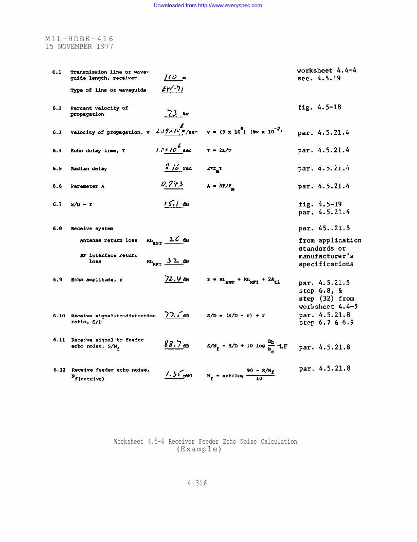
MIL-HDBK-41615 NOVEMBER 1977
Worksheet 4.5-6 Receiver Feeder Echo Noise Calculation (Example)
4-316
Downloaded from http://www.everyspec.com

MIL-HDBK-41615 NOVEMBER 1977
4-317
Worksheet 4.5-7 Calculate Median Total Noise Performance (Example)
Downloaded from http://www.everyspec.com

MIL-HDBK-41615 NOVEMBER 1977
4-318
Worksheet 4.5-8. Calcuate Short-Term Noise Performance (Example)
Downloaded from http://www.everyspec.com

MIL-HDBK-41615 NOVEMBER 1977
4-319
Worksheet 4.5-8. Calculate Short-Term Noise Performance (continued)
(Example)
Downloaded from http://www.everyspec.com

Worksheet 4.5-10
MIL-HDBK-41615 NOVEMBER 1977
4-320
Downloaded from http://www.everyspec.com

Worksheet 4.5-11
MIL-HDBK-41615 NOVEMBER 1977
4-321
Downloaded from http://www.everyspec.com

THIS PAGE BLANK
4-322
Downloaded from http://www.everyspec.com

MIL-HDBK-41615 NOVEMBER 1977
CHAPTER 5
FACILITY DESIGN
SECTION 5.0 INTRODUCTION,
5.0.1 In the previous chapters of this handbook, guidelines were
provided to the design engineer for site selection, performance
of surveys, and accomplishing the necessary calculations for path
performance predictions. This chapter provides the facility
design engineer with guidelines for arranging facilities and
equipment on the selected site, developing installation
specifications and instructions, and specifying hardware
necessary for installation of the facility. The criteria
contained in this chapter should be considered only as an
illustration. Latest issues of applicable military standard
should always be consulted for the definitive criteria that are
in current use. Those responsible for recommending site
selection and conducting site surveys for line-of-sight microwave
communications stations should consult DCA Circular 370-160-3,
Site Survey Data Book for Communications Facilities, November. — ——...—...—..—.——— -—- —-—.— -.
19/1, including Supplement 3, Change 2, titled Line-of-Sight
Station, dated July 1972.
5-1
Downloaded from http://www.everyspec.com

MIL-HDBK-41615 NOVEMBER 1977
SECTION 5.1 SITE PLANNING.
5.1.1 General.
5.1.1.1 This section is intended to contain information on all
the usual aspects of planning a microwave communications station.
Not everything discussed here will apply in every situation. The
most extensive site planning is ordinarily done for an
installation that will be new, a large communications hub, in an
undeveloped area and utilized solely for microwave
communications. If the microwave components are to be located at
a new, multipurpose site, the microwave engineer need only
provide his specialized requirement to the office directing
overall planning. If an existing site (and structure) is to
accommodate microwave communications, it Will be necessary only to
modify the site/building plan to include the addition of
microwave equipment and plant. Once a particular site or
location is chosen for a new microwave radio facility,
specifications and instructions for preparation of the site must
be generated. The content of the installation specifications
must be such that a general contractor/ qualified Government
personnel can accomplish the necessary site preparation, install
the equipment and place it into operation. If the work is to be
implemented by contractual actions, the specifications must
comply with the appropriate procurement regulations in both
5-2
Downloaded from http://www.everyspec.com

MIL-HDBK-41615 NOVEMBER 1977
format and content. In many cases the method of implementation
is not known at the time the specifications are written; that is,
whether the method of implementation will be contractual or
organic. Therefore the specifications should generally be
written so that they may be used in either case.
5.1.1.2 The bulk of the specifications will be in the form of
drawings supplemented by written specifications. These
specifications define those aspects of the work that can be
adequately described in words or cannot be easily illustrated.
The following areas of activity should be covered for total
development and construction of a communications station:
a. Site layout and plot plan.
b. Access roads and parking areas.
c. Site preparation, clearing and grading (maximum slope of
5 percent)
d. Building design.
e. Water supply and sanitation systems.
f. Antenna footings and/or structures.
,5-3
Downloaded from http://www.everyspec.com

MIL-HDBK-41615 NOVEMBER 1977
g. Prime and auxiliary power.
h. Heating, air conditioning and ventilating.
i. Site security fencing and lighting=
j. Real estate requirements.
5.1.1.3 Written specifications must be accurate, complete, and
concise. They should define the extent of the work, specify the
materials to be used, and establish responsibility for the
performance of work. In some cases part of the work may be
performed at more than one site by the same activity, whether
Government or contractor. In these cases the written
specifications may have general clauses applicable to all sites
and specific clauses applicable to individual sites.
5.1.1.4 A set of installation specifications will be required
for each microwave radio relay station. Individual site
specifications will be influenced by the present requirements of
the overall system and of the prospects for future expansion of
the system. These requirements are derived from system plans and
specifications.
5.1.1.5 The cost of future expansion can be reduced considerably
by taking reasonable effort to ensure that: adequate space is
5-4
Downloaded from http://www.everyspec.com

MIL-HDBK-41615 NOVEMBER 1977
available in the building or additional space can be made readily
available; the power equipment is adequate for future needs; and
the initial equipment is so located that rearrangement, rewiring,
and modifications are reduced to a minimum.
5.1.1.6 Where new construction is planned for the exclusive use
of the LOS communications facility, considerable thought should
be given to the use of the same type and size of buildings at a
number of sites with similar missions. Site adaptation of a
basic definitive design is common practice in the design and
construction business and this practice is often used by the U.S.
Government.
5.1.2 Site Plan.
5.1.2.1 Development of site plans require close coordination of
all aspects of civil and communications systems engineering to
determine the optimum site configurations. The following factors
should be considered when optimizing the site layout:
a. Site topography.
b. Available area.
c. Size, number, and types of buildings.
5-5
Downloaded from http://www.everyspec.com
MIL-HDBK-41615 NOVEMBER 1977
d. Direction and number of transmission paths.
e. Size, number, and height of antennas and supporting
structures.
f. Projections or obstructions to radio paths.
5.1.2.2 The preparation of the site plan should be concurrent
with the planning of the equipment building layout, since the
orientation and location of the tower and equipment building may
influence equipment layout design.
5.1.2.3 A typical site layout should concentrate on making the
equipment building the center of site operations. The antenna
structures should be placed as close to the equipment building as
possible, consistent with design codes and standards to minimize
the transmission line lengths required between equipment and
antennas. Figure 5.1-1 is an example of a site layout.
5.1.2.4 The number and direction of transmission paths specified
normally determine orientation of the equipment building with
respect to the site and the tower. A power generator building
may be used separately from the equipment building, but is
located sufficiently close to minimize power cable voltage drops
between generators and equipment. It usually requires less
effort and cost to collocate the power generators/equipment in
5-6
Downloaded from http://www.everyspec.com

MIL-HDBK-41615 NOVEMBER 1977
5-7
Downloaded from http://www.everyspec.com

MIL-HDBK-41615 NOVEMBER 1977
the same building with the electronics equipment; in this case
the building should have a specially designed room for generators
to minimize noise and vibration and any hazards such as toxic
fumes and fire. Ordinarily, a generator is secured to the floor
through vibration mounts. The engine exhaust pipe to the outside
is quieted by a muffler placed close to the engine. Fuel storage
areas should be located where the peak RF power density is less
than 5.0 watts per square centimeter, In those cases where it is
necessary for the personnel to live on site, every effort should
b e made to provide as much isolation as possible between the
living area and the work area. In many cases, physical isolation
alone is not sufficient for health and safety of personnel;
therefore, if required, sound absorption material should be
installed on walls separating work and living areas. In the case
of a small installation this may have to be accomplished in the
same building; while, with a large installation it would be
preferable to have separate buildings.
5.1.2.5 The topography of the site area often has an important
effect upon the site layout. When necessary, compromises in site
layout are effected to keep site preparation and grading within
reasonable limits.
5.1.2.6 If the microwave station being planned requires
attendant personnel, it will be necessary to locate water for
their use. An adequate supply of safe water for domestic use and
5-8
Downloaded from http://www.everyspec.com

MIL-HDBK-41615 NOVEMBER 1977
fire protection must be available at all times. Domestic water
requirements at an installation include drinking, cooking,
washing, bathing, sewage disposal, and possibly a small amount
for watering cultivated areas. Most repeater sites do not
require or justify elaborate systems and can be supplied by water
trailer, community water main, etc. Terminal sites will usually
be located in proximity to major compounds and can be supplied by
the existing system.
5.1.2.7 The final site plan should show:
a. Site boundary and property lines.
b. Location and dimensions of buildings, tower, foundations
fuel tanks, driveways, walks, retaining walls~ drainage
structures, water supply and sewage disposal (if required),
fencing, access roads and parking areas.
c. Baseline and bench marks.
d. Elevations, azimuths, and coordinates for the center of
each antenna.
e. Underground utilities.
f. Underground services.
5-9
Downloaded from http://www.everyspec.com

MIL-HDBK-416 15 NOVEMBER 1977
g. Existing buildings facilities and roads.
h. Magnetic North direction/orientation.
i. A vicinity map.
5.1.2.8 Developing a site plan is the responsibility of the
civil engineering authority based upon the communications system
requirements as follows:
a. Where services and consequently facilities are required.
b. Type and volume of equipment space determined by amount
and kind of equipment and physical support required.
c. The degree of operation and maintenance required
governing personnel requirements.
d. Environmental and power requirements.
e. Location and alignment of antennas.
The LOS communications engineer has the responsibility of
gathering this data and translating it into requirements civil
engineering can use in preparing the site plan. For existing
5-10
Downloaded from http://www.everyspec.com

facilities a site plan should already exist and should be revised
to show new construction. When the project involves the
installation of equipment inside an existing, properly identified
building, it should not be necessary to include a site plan with
the engineering specifications.
5.103 Access Roads.
5.1.3.1 A preliminary engineering study, prior to the
development of all weather site access roads and parking areas,
should take into account vehicular traffic demands. Although the
final access road position will depend primarily on site
location, layout, and topography, the final design should offer
direct routing, adequate right of way visability, good foundation,
proper drainage, and degrees of curvature and grade consistent
with good highway engineering practice.
5.1.4 Site Preparation.
5.1.4.1 The written specifications should include instructions
concerning the clearing of the site and the extent of excavation,
backfilling, and grading. They should also include instructions
for the construction of driveways, walks, retaining walls, and
fencing.
5.1.5 Building Design.
5-11
MIL-HDBK-416
15 NOVEMBER 1977
Downloaded from http://www.everyspec.com
MIL-HDBK-41615 NOVEMBER 1977
5.1.5.1 The size of a building used to house microwave equipment
depends upon the station function. In particular the following
factors must be considered.
a. Size and quantity of required equipment and possible
future equipment.
b.
c.
d.
Necessary working space around equipment.
Required space for maintenance purposes.
Personnel requirements (desk space, sanitary
facilities).
e. Housing of power equipment.
5.1.5.2 At some sites~contemplated use of existing buildings
necessitates investigation of load bearing capabilities of the
floor. The need for heavy antenna mounts on the building may
require building reinforcement.
5.1.5.3 At remote sites new buildings may be erected. The type
of construction depends upon physical conditions peculiar to the
locality, and availability and relative cost of construction
materials. Other considerations include the required strength
5-12
Downloaded from http://www.everyspec.com

MIL-HDBK-41615 NOVEMBER 1977
and durability of the building, and necessary maintenance.
Additional factors affecting the type and strength of a structure
are: climatic conditions, temperature range, wind velocities,
and amount of rainfall and/or snowfall. Transportation and
handling costs and site accessibility affect the selection of
construction materials. Local codes governing the use of certain
materials and methods of construction must be investigated. The
availability of skilled labor may be a deciding factor. In areas
where a considerable amount of snow and high winds are to be
expected, such as mountain top sites, enclosed walkways should be
provided between buildings. Also suitable provisions should be
made to ensure that the access road can be kept open.
5.1.5.4 For small stations the above requirements can be met by
using either sheet metal or masonry construction. Sheet metal
buildings can be prefabricated, easily erected, and readily
enlarged or relocated if need be. Masonry buildings have greater
durability.
5.1.5.5 For each building an Architectural and Engineering (A&E)
drawing package that includes the following categories of plans
should be prepared:
a. Civil Plans - site, grading and utility plan, sections,
profiles, details, and boring logs.
5-13
Downloaded from http://www.everyspec.com

MIL-HDBK-41615 NOVEMBER 1977
b. Architectural Plans - floor plans, elevations, details,
schedules etc.
c. Structural Plans - foundations, roof and wall sections,
elevations construction details, etc.
d. Electrical Plans - electrical distribution, power
distribution, control panels, lighting schematics, grounding
plans and details.
e. Mechanical Plans - heating, ventilation, and air
conditioning plans, diagrams and details.
f. Plumbing Plans - water supply and sanitation facilities
plans, diagrams and details.
5.1.5.6 The equipment to satisfy the initial communications
requirements determines the floor space requirements of the
station. The kind and quantity of equipment as well as the type
of operation dictates space to be provided for the electronics
bays plus power and other corollary equipments and for personnel.
If at all practical the equipment layout should be planned in
such a manner as to afford sufficient space for the installation
of equipment capable of handling the maximum projected traffic
load. The initial equipment layout should be such that ultimate
expansion of the station facility can be accomplished without
5-14
Downloaded from http://www.everyspec.com

MIL-HDBK-41615 NOVEMBER 1977
extensively rearranging already installed equipment. Allowance
of space for future equipment can be determined if specific
equipments for future installation are known; otherwise, an
estimate based upon the requirements of similar equipments should
be made. When planning a new communications facility, the
engineer should take into consideration the possibility of
installing additional equipment in the floor space being
provided. The expansion capability for future growth should be
determined on a site-by-site basis, based on many factors, such
as anticipated need, cost, etc. In addition, its design should
include a capability to enlarge the station from at least one
wall. Specific building design criteria associated with
communications station requirements are discussed in the
following paragraphs.
5.1.5.7 Building of single story, rectangular construction are
most common for exclusive utilization by microwave radio
communications installations. Equipment buildings may be
physically separated from other site buildings such as power
generator buildings and living quarters. When a single building
is employed, one end would normally be used as the equipment
room, the center of the building for maintenance and storage, and
the opposite end for administrative functions at the station. A
good way to segregate a single, all-purpose, microwave radio
communications building is to have one wing for communications
equipment, a second wing for power generators, and others for
5-15
Downloaded from http://www.everyspec.com

living quarters and offices. Storage and maintenance should be
situated close to the communications equipment area. Buildings
with multiple stories also afford easy segregation of functions.
5.1.5.8 To determine the space requirements and layout of the
building, floor plans should be developed showing the location of
all equipment in the operations and maintenance areas.
Requirements for spare parts storage space are determined by the
types of equipment, and level maintenance to be performed at the
station. Consideration should be given to the reduction of spare
parts storage requirements resulting from improved equipments,
and streamlined maintenance and supply technique now being
employed. Space requirements for administrative and sanitation
facilities are determined from the number of personnel programmed
for normal operation and maintenance duty at the station.
5.1.5.9 At least one outside door to the equipment room, capable
of passing the largest single component that may be moved into
the station is required. A loading ramp or dock must be provided
immediately outside this door to facilitate loading and unloading
heavy equipment from trucks. If the building floor is at ground
level, hardstand should be provided from the drive to the
equipment room freight door.
5.1.5.10 Ceilings in the equipment area should be at least 10
feet above the floor level for adequate ventilation of standard
5-16
MIL-HDBK-41615 NOVEMBER 1977
Downloaded from http://www.everyspec.com

MIL-HDBK-41615 NOVEMBER 1977
eight-foot equipment racks. This height also provides proper
diffusion of light throughout the equipment area from ceiling
luminaries. In the case of large installations a unistrut grid
with 4 ft spacing is normally provided below the ceiling to
provide support for the various cable racks or trays that may be
required above the equipment bays for the equipment
interconnecting cables and power distribution lines.
5.1.5.11 The building floor must be designed to support the
heaviest item of equipment likely to be placed upon it as well as
the total weight of all equipment on it. Overall, the floor
should support the entire weight of all stationary and wheeled
equipment, personnel, supplies, storage, and non-load bearing
walls, and should provide sufficient overload factors to
accommodate the installation of heavier or additional
communications equipment for future expansion. T O do this a
minimum floor loading of 100 pounds per square foot is usually
considered adequate.
5.1.5.12 Provisions must be made in the walls, ceiling and roof.
of the equipment buildings for installation of transmission lines
running to the outside of the building. These exit ports require
“tailoring" to the installation at each station, and may include
RF shielding.
5.1.5.13 Some microwave stations will require the installation
5-17
Downloaded from http://www.everyspec.com

MIL-HDBK-41615 NOVEMBER 1977
of various types of hardware on the roof of the building such as
roof ventilators (added by the building construction authority)
and root mounted antennas (as required and specified by microwave
LOS engineer) . A roof plan should be provided showing all
pertinent details that will be required by the personnel
responsible for the installation of the station. There are
usually two major factors that will determine the specific
location for the placement of antennas on top of a building. The
first will be the location of the tower mounted reflector or the
adjacent station to which the antenna will be directing a signal,
and the second will be the relative location of the microwave
equipment within the building. Having the antenna in proximity
to the microwave equipment will avoid unnecessarily long
waveguide runs. It should be recognized thought that the tower
mounted antenna with transmission line is preferred over an
antenna-to-tower mounted reflector (periscope) configuration.
5.1.5.14 For a station to be equipped with no break power, a
room will have to be provided for a battery bank plus suitable
space for a rectifier-charger unit.
5.1.5.15 The design of the interior lighting will be according
to recommendations of the Illuminating Engineering Society (IES)
Lighting Handbook. Specific location of the equipment cable
racks, waveguide runs, unistrut grid, work benches, desks and
consoles must all be considered in the design of the lighting
5-18
Downloaded from http://www.everyspec.com

MIL-HDBK-41615 NOVEMBER 1977
system. Battery power emergency lighting is required throughout
the building.
5.1.6 Station Ground.
5.1.6.1 The DCA Notice 310-70-1, entitled "DCS Interim Guidance
on Grounding, Bonding, and Shielding”, provides guidance for
designing a good grounding system. The elements of a ground
system for a communicantions standard are an earth electrode
system, power grounding network, safety grounding network,
lightning protection grounding network, a facility grounding
network. and a Low frequency signal grounding network.
5.1.6.2 Earth Electrode System. The earth electrode system
provides electrical contact with earth and is the common
interconnection point for all the various grounding networks.
The higher the soil resistivity, the more complex (and expensive)
will be the electrode system necessary to achieve low resistance
to earth. Two typical configurations of earth electrode systems
are as follows:
a. Ten-foot ground rods installed at 20-foot intervals
around the perimeter of the structure provide good utilization of
the effective radius of the rod while providing several points of
contact with the earth.
5-19
Downloaded from http://www.everyspec.com

MIL-HDBK-41615 NOVEMBER 1977
b. In regions of shallow bedrock, vertical ground rods may
be ineffective and horizontal grids, wires, or plates must be
used. A typical ground system of this type may consist of buried
copper radials, extending in all directions from the building
center, and a single ground point extended through the floor of
the equipment room for connection of the electronic equipment.
5.1.6.3 Power Grounding and Safety Grounding Network. This is
an integral part of the power system and should be done in
accordance with the National Electrical Code.
5.1.6.4 Lightning Protection Grounding Network. This is an
integral part of the construction of the building or antenna
support structure. (See paragraph 5.4.2.3 on lightning
protection.)
5.1.6.5 Facility Grounding Network. This network is a
conductive grid providing multiple low resistance paths between
any two points within the structure and between any point in the
structure and the earth electrode system. The facility grounding
system is to be separated from the low frequency signal grounding
network, described in 5.1.6.6, except f o r t h e common
interconnection made at
electrode system.
5.1.6.6 Low Frequency
the main ground plate of the earth
Signal Grounding. The low frequency
5-20
Downloaded from http://www.everyspec.com

MIL-HDBK-41615 NOVEMBER 1977
signal grounding network is used to furnish a single-point
reference for low frequency signals~ minimize power frequency
noise levels in sensitive low frequency equipments and provide
for fault protection and static discharge of otherwise isolated
networks. Low frequency signals are defined as those with
frequencies less than one megahertz.
5.1.6.7 Ordinarily, a microwave radio is interconnected with the
facility grounding system. Frequency or time division
multiplexing if included with the installation, should have its
drop side grounded to the low frequency signal grounding network.
The baseband cable between the radio and multiplexer or between
radios at a repeater station should have its shield grounded to
the low frequency signal grounding network if conducting signal
currents with frequencies not exceeding one megahertz, or to the
facility grounding system with frequencies over one megahertz.
At small repeater stations, it may not be practical to have a
separate low frequency signal grounding network; then the
baseband cable shield would connect to the facility grounding
network regardless of frequency. Whatever method employed,
extreme care and sound judgement must be exercised because
baseband cables are a critical means by which noise is introduced
into radio systems. Grounding conductors will be stranded,
insulated copper wire and adequately sized to conduct all
currents likely to be imposed. Main grounding leads are usually
run on the cable rack, tray or in trenches with signal cables.
5-21
Downloaded from http://www.everyspec.com

MIL-HDBK-41615 NOVEMBER 1977
Taps of smaller size wire are run from the main grounding lead to
individual equipments. Connections to this main grounding lead
are made with suitable lugs, pressure connectors or clamps.
5-22
Downloaded from http://www.everyspec.com

MIL-HDBK-41615 NOVEMBER 1977
SECTION 5.2 EQUIPMENT LAYOUT.
5.2.1 General.
5.2.1.1 Equipment layout should be standardized among the
facilities comprising a communications system insofar as
possible. In determining the layout, the necessary access for
installation ~ maintenance and operation should be a major
consideration. This would include such considerations as
provision of adequate space between rows of equipment to allow
for opening of cabinet doors or sliding out modules for
maintenance. Another major but less important consideration is
providing the shortest and most direct waveguide runs
practicable.
5.2.1.2 Other equipment layout considerations include minimizing
interbay cabling runs~ provision for future expansion, and
providing easy access for maintenance and operational
convenience ~ etc. Sometimes the electromagnetic incompatibility
of various types of equipment or inadequate ventilation for
personnel and equipment can be problems. Equipment of the same
type or with similar functions are usually grouped together
except where impractical due to size and specific requirements of
a station. In a typical situation radio/ multiplex equipment,
crypto equipment, and technical control equipment are each
grouped in separate rooms with other rooms being used for
5-23
Downloaded from http://www.everyspec.com

MIL-HDBK-41615 NOVEMBER 1977
administration and maintenance.
5 .2.1.3 Human engineering can be another factor of concern in
laying out equipment. Equipments should be properly grouped
according to their functions and interoperation. Care and
thought should be given to the arrangement of meters, test
equipment, jack fields, indicating lights, etc. to assure they
are placed at the approximate eye level, thus allowing more rapid
and convenient use. Equipment should not be mounted at the
bottom of a bay, if it can be easily damaged or if its size and
shape will interfere with power boxes or other hardware at the
bottom of the cabinet or rack. Fortunately, most microwave radio
equipment comes fully packaged with all components already
mounted within the cabinet or rack.
5.2.1.4 It is advisable to arrange equipment within the
equipment room in such a manner that expansion of the building
will not necessitate rearrangement of existing installed
equipment. A satisfactory arrangement is to align the equipment
in rows on both sides of the building, with sufficient clearance
between the rear of the equipment and the wall for use as an
access/service area, and to provide an aisle between the front
panels of facing equipment. The point of entry for antenna
waveguide and possible transmission lines for this arrangement
will generally be along the sides of the building. The end wall
of the equipment room opposite the mechanical, generator, or
5-24
Downloaded from http://www.everyspec.com

MIL-HDBK-41615 NOVEMBER 1977
toilet facilities should be considered as the direction for
future building expansion. Therefore, installation of equipment
at this room location should be avoided if possible. The end
wall location may also be considered for use as an equipment
ingress opening, by removal of wall panels, to permit
installation or removal of equipment.
5.2.1.5 In determining floor area requirements for the
communications equipment, a number of factors must be considered.
The most important factor is that of providing sufficient space
to suitably house all of the equipment and at the same time allow
adequate clearance for ventilation and permit ready access for
maintenance. When placing each piece of equipment, frequent
reference should be made to the rack assembly and outline
dimensional drawings with special regard to minimum wall
clearance requirements, spacing between equipments, power and
antenna connection points, and minimum radius requirements for
the removal of protective housings and opening of maintenance
access doors. Approximately three feet of clearance space, at a
minimum, should be allowed in front of and to the rear of an
equipment bay. If a bay does not permit rear access to
equipment, the bay may be installed with no clearance on the back
side, i.e., against a wall or back to back with other bays,
ventilation requirements not withstanding.
5.2.1.6 The operational plan of the station must be studied to
5-25
Downloaded from http://www.everyspec.com

MIL-HDBK-41615 NOVEMBER 1977
determine the communication circuit requirements when placing
each component or rack assembly. In small stations it is
recommended that the equipment be aligned in a row along one or,
if need be, both sides of the building with sufficient space
between to accommodate a normal floor traffic pattern. However,
this type of layout will generally not be suitable in stations
where large quantities of equipment are involved. In the larger
station the most practical layout is usually one in which the
equipment is aligned in bays across the width of the room, with
sufficient space between bays to permit free access to each rack
assembly.
5.2.2 Installation Plans.
5.2.2.1 After the equipment layout has been determined,
installation plans can be developed. Installation plans contain
all the information and instructions required to accomplish all
aspects of the installation under the cognizance of the microwave
communications system engineering activity. Some typical plans
for specifying installations are explained in this section. The
format of these engineering plans may vary from agency to agency.
5.2.2.2 Floor Plans. Floor plans provide a pictorial
representation of equipment placement as well as administrative,
maintenance and storage areas. All required dimensions must be
specified on the floor plan with sufficient detail included
5-26
Downloaded from http://www.everyspec.com

MIL-HDBK-41615 NOVEMBER 1977
relative to obstructions, to preclude interference with equipment
placement.
5 .2.2.3 Cable Rack Layout. Cables for interconnecting and
terminating equipments are distributed by one or a combination of
three methods: overhead open rack, overhead enclosed tray, or
raised floor/floor trenches. Selection of one or a combination
of these methods is dictated by the individual station equipment.
Layout drawings should be
a. Overhead view
plan.
b. Detailed
three-dimensional views
prepared which depict:
of cable layout superimposed on floor
two-dimensional and perspective
of cable arrangements such as elbows,
splitsf tee sections~ reducing sections and dropouts.
c. Equipment distribution frames and AC branching panel
access details.
d. Rack/Cable support and hardware list of materials keyed
to layout and details.
5.2.2.4 Cable Termination Lists. All VF and slow speed data
signal equipment in a communications station is wired to a
distribution frame (DF) as a common terminus for interconnection
5-27
Downloaded from http://www.everyspec.com

MIL-HDBK-41615 NOVEMBER 1977
of circuits ingressing/ egressing all communications equipment.
Information for terminating cables on a distribution frame is
provided by cable termination lists. Each wire is given a
specific punching assignment on a specific distribution frame
termination block. A simple radio repeater station likely would
not utilize a distribution frame, and the cable list would
reflect runs directly from equipment to equipment. The microwave
engineer would be concerned with wiring to the DF only to
terminate the drop circuits on multiplexing equipment or to cable
order wire and control and fault alarm circuits. See
MIL-STD-188-310, "Subsystem Design and Engineering Standards for
Technical Control Facilities”, for a description of the breakout
of individual circuits and their flow through a communications
station.
5.2.2.5 Cross-Connect Lists. Assuming the station is large
enough to have a distribution frame, cross-connect lists are used
to identify or explain the connection of jumper wires on a
distribution frame. This cross-connect list is required to
interconnect a particular equipment group in a prescribed manner.
Cross-connections could be the responsibility of the operating
agency for expansion or replacement of equipment in an existing
facility. For a turn-key project the cross-connections are part
of a complete installation.
5.2.2.6 Power Distribution Drawings. Power wiring from the
5-28
Downloaded from http://www.everyspec.com

MIL-HDBK-41615 NOVEMBER 1977
power distribution panel to each equipment is completely
described by the power distribution drawings, including the
method to be used by the installer in wiring individual
electronic equipments to the power source. They specify such
features as:
a. Type and size of wire to be used.
b. Routing of wires.
c. Specific circuit breakers (or fuses) associated with
each equipment.
d. Diagrams of each panel board, indicating equipment
connected to each circuit breaker, rating of the breaker and the
load connected to each breaker.
e. For AC, tabulation of total loads on each phase of the
panel feeder and the total load on all phases (of more concern to
the power engineer than the communications engineer).
f. Materials required to accomplish installation of the
power wiring.
g. Required power for each equipment.
5-29
Downloaded from http://www.everyspec.com

MIL-HDBK-41615 NOVEMBER 1977
5.2.2.7 Grounding Drawings. The station grounding system is
shown by a grounding diagram that specifies ground system
routing~ cable size~type and position of all ground connectors
and materials required to install the grounding system. Design
of the station ground is outlined in paragraph 5.1.6.
5.2.2.8 Equipment Installation Drawings. All necessary
information to accomplish installation of an equipment is
provided by these drawings. They contain installation details
peculiar to a specific equipment and illustrate the planned
procedures for accomplishing each portion of the installation
effort. When different equipments require the same basic
installation information, a common installation drawing may be
used. In either case materials required to install the equipment
should appear.
5.2.2.9 Transmission Line Layout Drawing. This drawing shows
the details of the RF transmission line and its routing. It
specifies the size components to be used at each point along the
route and where bends and flexible sections are to be located.
The location of gas barriers and the arrangement of the
pressurizing system should be shown.
5.2.2.10 List of Materials. A composite listing of materials
required to install the facility should be included in the
installation plan.
5-30
Downloaded from http://www.everyspec.com

5.3 PRIME AND AUXILLARY POWER.
5. 3.1 General.
5.3.1.1 Power systems shall be engineered to provide continuity
of vital communications. The availability/reliability of the
power system shall be based upon the operational requirements of
the communication systems. The minimum electrical performance
parameters shall be in accordance with MIL-HDBK-411.
5.3.2 Desc ription of electrical power systems: The power
systems
a.
b.
c.
for a LOS site shall consist of the following:
Primary Source: Commercial or "Class A".
Emergency: "Class C".
Floating Battery Plant: "Class D".
5.3.2.1 Primary Source: When available, commercial power will
be utilized as the primary source. At isolated locations where
the cost of providing commercial power is not justifiable, a
"Class An plant shall be provided.
5.3.2.2 Emergency Source: A "Class C" engine driven generator
5-31
MIL-HDBK-41615 NOVEMBER 1977
Downloaded from http://www.everyspec.com

1MIL-HDBK-41615 NOVEMBER 1977
with automatic start and control unit is required to provide
power upon failure of the commercial source. The unit shall be
sized to provide power for the total site load. NOTE : "Class C"
power is not required where “Class A“ on site power plants are
provided.
5.3.2.3 Floating Battery Plant "Class D”: A floating battery
plant is required to provide continuous power to the critical
technical loads. The system consists of batteres, rectifiers
inverters~ control panels~and distribution equipment. A minimum
of two rectifiers shall be provided with each system =Each
rectifier shall be sized for the full electronic tech load and
for charging the batteries. This system is normally provided
with the electronic equipment and is installed within the
communication facility.
5.3.3 Power control and fault alarm panel: A power control and
fault alarm panel for remote control and monitoring of the power
system (AC
shall be
building.
capability
and DC) with appropriate meters, relays, and switches
provided in the control area of the communication
This control and alarm system shall have the
of being remoted into the order wire system.
5.3.4 Fuel Storage Facility: The size of the fuel storage
facility shall be specified in MIL-HDBK-411.
5-32
Downloaded from http://www.everyspec.com

MIL-HDBK-41615 NOVEMBER 1977
5.4 TOWER REQUIREMNETS.
5.4.1 General.
5.4.1.1 This section is for providing the communications
engineer a description of the information required for a
structural engineer to design or specify a tower and foundation
adequate for its intended use. The information presented
includes structural design considerations, design safety
requirements, grounding for lightning protection and painting and
lighting requirements.
5.4.2 Structural Design.
5.4.2.1 Microwave towers may be either self supporting towers or
guyed towers. For permanent installations and main route high
density applications, self supporting towers are preferred. They
require less real estate than the same height guyed tower and
offer more flexibility in the location of the antennas providing
for possible future antenna relocation. For temporary or
tactical applications, guyed towers may be more practical. The
real estate required for tower guys is somewhat variable but does
not usually exceed a circle with radius equal to tower height.
Towers can be designed for almost any height; however, economic
and practical considerate ions limit the maximum height to
approximately 300 ft. or 100 meters for wideband communication
5-33
Downloaded from http://www.everyspec.com

MIL-HDBK-41615 NOVEMBER 1977
use. This is not an absolute maximum but other alternatives
should be carefully considered if higher towers seem to be
required.
5.4.2.2 Tower and foundation design are dependent upon four main
factors: (1) soil bearing capability at the specific location;
(2) the size and number of the parabolic antennas and their
location on the tower; (3) the meteorological conditions to be
expected; and (4) the maximum tower twist and deflection (see
section 4.4.30) that can be tolerated under worst conditions of
Wind loading (and ice loading it applicable). Design of the
required tower foundation is directly related to the tower design
and the specific soil conditions involved.
5.4.2.3 Tower loading is the resultant of all forceS acting on
the tower. Design of the tower must be such that with all
antennas and other required items mounted on the tower, it will
when subjected to maximum specified wind and ice conditions,
resist any deflection or twisting beyond a specified amount.
5.4.2.4 Since the net result of all the tortes on the tower are
also in effect transmitted to the foundation, it in turn must be
capable of distributing the force over a large enough area and
depth so as not to exceed the soil bearing pressure at any Point
and also to resist movement in any direction. The depth of the
foundation will be governed by the tower load and soil bearing
5-34
Downloaded from http://www.everyspec.com

MIL-HDBK-41615 NOVEMBER 1977
characteristics, but in colder climates, it is necessary to
extend the depth of the foundation below the frost line or to
firm ground.
5.4.2.5 The soil bearing capability, usually designated as a
pressure in pounds per square foot, is a determining factor in
the design of a tower foundation. Table 5.4-1 illustrates the
maximum soil bearing value for various types of soil conditions.
Unfortunately, the designation of the various soil conditions are
arbitrary in nature so the table should only be used as a rough
guide for preliminary estimates. Soil borings taken at the area
in question are normally required for a final design.
5.4.2.6 The following type of information must be provided by
the communications engineer in order for the tower designer to
adequately design a suitable tower and foundation combination.
a.
b.
c.
Size and type of antennas required and type of radomes.
Azimuth and elevation angles for each antenna.
Amount of adjustment required for alignment after
installation. (Normally, plus or minus 5 degrees in both azimuth
and elevation.)
d. Height above ground for each antenna.
5-35
Downloaded from http://www.everyspec.com

MIL-HDBK-41615 NOVEMBER 1977
Table 5 .4-l Maximum Soil Bearing Capabilit y
MATERIAL
BedrOCk (sound) without laminations
Slate (sound)
Shale (sound)
Residual deposits of broken bedrock
Hardpen
Gravel (Compact)
Gravel (loose)
Sand, coarse (canpact)
Sand, coarse (loose)
sand, fine (compact)
sand, fine (loose)
Hard clay
Medium clay
Soft clay
MAXIMUM ALLOWABLEBEARING VALUE(LB PER SQ FT)
200,000
70,000
20,000
20,000
20*000
10,000
8,000
8,000
6,000
6,000
2,000
12,000
8,000
2,000
5-36
Downloaded from http://www.everyspec.com

MIL-HDBK-41615 NOVEMBER 1977
e. Location of tower with respect to the building and their
corresponding orientations.
f. Beam widths of the antennas and permissible twist and
deflection of the tower that can be tolerated under maximum
expected wind and ice loading.
g. Type and number of waveguide runs required and power
cabling for feedhorm or radome heaters.
h. Requirements for tower lighting, obstruction lights,
lightning protection grounding systems, and painting.
i. Requirements for platforms to
antennas for maintenance and/or alignment.
allow access to the
j. Required means of access up the tower including required
personnel safety features.
k. Provisions for future antenna requirements.
l. Climatic details of the area involved.
m. Local restrictions and/or other constraints that may be
involved.
5-37
Downloaded from http://www.everyspec.com

MIL-HDBK-41615 NOVEMBER 1977
n. Soil conditions.
5.4.3 Tower Safety.
5.4 .3.1 Tower safety is concerned in two areas: (1) the safety
of personnel using the structure, and (2) the hazard imposed by
the tower to aircraft.
5.4.3.1.1 The hazard imposed to aircraft by the tower is
minimized in two ways: (1) painting and lighting, and (2)
restriction against tower installation. Painting and lighting is
covered by para 5.4.50 Restriction against installation is
covered by A FM 86-8, Airfield Clearance Criteria. For
installation in a foreign country, the siting engineer must check
for clear zone or height restrictions that may exceed those in
AFM 86-8.
5.4.3.1.2 The safety features required to protect personnel when
working on the tower must be included in the tower design.
Design requirements for ladders, stairs~ and elevated work
platforms are specified in OSHA, Volume I, General Industry
Standards. Requirements for ladder climbing safety devices are
stated in AFM 127-101 and OSHA, Volume I, General Industry
Standards.
5-38
Downloaded from http://www.everyspec.com
MIL-HDBK-41615 NOVEMBER 1977
5.4.4 Lightning Protection for Towers.
5.4.4.1 Lightning protection must be considered as part of each
tower installation. Lightning protection for towers shall be in
accordance with the latest edition of Underwriters Lab (UL),
Pamphlet 96A, Lightning Protection Systems. Common grounding of
lightning protection ground with existing facility grounding
systems shall be provided. Air terminals, down leads, and a low
resistance ground are basic requirements for adequate protection
of towers. Materials for this system will meet requirements of
UL 96. Waveguide on tower will be grounded before it enters
building.
5.4.4.2 Any and all equipment mounted on a tower shall be
fastened so that it is effectively grounded through the tower.
On structures provided with obstruction lights, it may be
desirable to place suitable lightning surge arrestors on wires
supplying these lights.
5.4.4.3 The maximum permissible ground resistance to true earth
of earth electrode system for tower prior to connection to down
leads is 10 ohms. However, if 10 ohms is impossible due to tower
sitting on a solid rock location, an extensive wire counterpoise
system with radials (copper cables) extending from corners of
counterpoise may be substituted versus an earth electrode system.
Minimum Number 2 AWG bare copper wire should be used for
5-39
Downloaded from http://www.everyspec.com

MIL-HDBK-41615 NOVEMBER 1977
counterpoise and radial ground system.
5.4.5 Painting and Lighting Requirements,
5.4 .5.1 The guidelines and requirements contained in this
section apply primarily to installations within the United
States. In overseas installations~regulations imposed by
cognizant military and/or government agencies must be studied.
To prevent excessive hazards to air commerce, antenna towers and
similar structures must be marked in such a way as to make them
conspicuous when viewed from aircraft. The type of marking to be
used depends in part on the height of the structure, its location
with respect to other nearby objects, and its proximity to
aircraft traffic routes near landing areas. Requirements and
specifications for marking and lighting potential hazards to air
navigation have been established through joint cooperation of the
Federal Aviation Agency, Federal Communications Commission,
Department of- Defense and appropriate branches of the
broadcasting and aviation industries. The specifications
determined by these groups aid in the final decision as to
whether a structure constitutes an obstruction to air navigation.
When conducting the preliminary site survey, it is advisable to
determine the prevailing ordinances concerning such structures,
and perhaps to discuss them with local government and building
authorities. When dealing with locations within the continental
limits of the United States, the latest copies of Government
5-40
Downloaded from http://www.everyspec.com
MIL-HDBK-41615 NOVEMBER 1977
Rules and Regulations, FCC Form 715, FCC Rule, Part 17, and FAA
Standards for Marking and Lighting Obstructions to Air
Navigation, with all revisions should be consulted. These rules
not only apply to specifications for antenna structures, but also
set forth the forms which must be submitted to the FCC, FAA, and
Us. cost and Geodetic Survey (FCC Form 401A Revised, FAA Form
117, FAA Form ACA-114, and G&GS Form 844).
5.4.5.2 In order to warn airmen of the presence of obstructions
during daylight hours in good weather conditions, all structures
that may present a hazard to air commerce will be painted from
top to bottom in accordance with requirements of the latest
edition of FAA-AC 70/7460-1( ).
5.4.5.3 Both the FCC and FAA lighting specifications are set
forth in terms of the heights of the antenna structures. The
requirements for towers and obstructions will be determined from
FAA Specifications specified in the latest edition of AC
70/7460-1( ). The specifications further stipulate that
placement of the lights on either square or rectangular towers
shall be such that at least one top or side light be visable from
any angle of approach. When a flashing beam is required, it
shall be equipped with a flashing mechanism capable of producing
not more than 40 nor less than 12 flashes per minute with a
period of darkness equal to one-half the luminous period.
5-41
Downloaded from http://www.everyspec.com
MIL-HDBK-41615 NOVEMBER 1977
5 .4.5.4 When the tower structure is in the process of
construction, the FCC and FAA require that temporary lights,
consisting of at least two 100-watt lamps enclosed in aviation
red globes be displayed at the top of the structure from sunset
to sunrise. Lights must also be installed at intermediate
heights, if necessary IAW FAA requirements.
5.4.5.5 The FCC requires that tower lighting be exhibited during
the period from sunset to sunrise unless otherwise specified. At
unattended microwave installations, a dependable automatic
obstruction-lighting control device must be provided. A
light-sensitive control device will be used to control the
obstruction lighting in lieu of manual control. This requirement
will be met in microwave installations by employing a tower
lighting kit. These kits apply power to the lights when the
north skylight intensity is less than approximately 35 foot
candles and disconnect the power when the north skylight
intensity is greater than approximately 58 foot candles.
5.4.5.6 To insure the proper operation of tower lights, the FCC
specifies that the lights be inspected at least once every 24
hours; the inspection can be performed either by direct
observation or by observation of an automatic and properly
maintained indicator designed to register failure of such lights.
Where obstruction lighting is not readily accessible for periodic
inspection~the rules permit use of electric signaling devices
5-42
Downloaded from http://www.everyspec.com

MIL-HDBK-41615 NOVEMBER 1977
to indicate lamp failure. Should the fault alarm system register
a failure in obstruction or beacon lighting, the failure must be
reported to the nearest Airways Communication Station of the
Federal Aviation Agency. The FAA must be notified of any code
beacon, rotating beacon, or top light failure if not corrected
within 30 minutes after failure.
5-43
Downloaded from http://www.everyspec.com

MIL-HDBK-41615 NOVEMBER 1977
5.5 ENVIRONMENTAL CONTROL
5.5.1 General. This section provides as general guidance and
assistance to the mechanical environmental design engineer to
indicate the basis for design which will be supplemented by
specific design criteria based on the technical characteristics
of the equipment concerned. It is not the intent to dictate
specific design approaches but to portray general guidelines to
be considered. Each individual mission will require initiative ~
imagination? and sound engineering judgement to meet the
circumstances involved. Radical departures from the standards
and guidelines noted herein will require coordination of DCA and
the appropriate Military Department Field Engineering Office.
5.5.2 Environmental Control Systems. Environmental control as
used in this handbook includes all equipments used for cooling,
heating, ventilation, humidification, dehumidification,
filtration, pressurization, and distribution of air and the
control thereof. Environmental control as defined here is for
the communications equipment and all systems, personnel and
facilities that directly support these items.
5.5.2.1 This section provides general guidance for the selection
of desired environmental conditions. The information contained
herein will have to be supplemented by more specific
environmental design criteria based on the requirements of the
5-44
Downloaded from http://www.everyspec.com

MIL-HDBK-41615 NOVEMBER 1977
communications equipment to be installed.
5.5.2.2 When installed equipments operating range requires
environmental conditions that are different than those outlined
in this document, those requirements shall be used as a basis for
design; however, every effort should be made to minimize life
cycle costs.
5.5.2.3 For further design guidance, refer to the design manuals
of DOD design and user agencies and the Defense Communications
Agency (DCA). The latest edition of the American Society of
Heating, Refrigeration and Air Conditioning Engineers Guide and
Data Books - fundamentals, applications, systems, and equipment
volumes - should be followed as a basic reference for system
design except where modified by more specific criteria including
MIL-HDBK-411.
5.5.3 Design Conditions - Electronic Equipment Spaces.
5.5.3.1 Outside conditions to be used as a basis for design
shall be taken from the Army, Navy, and Air Force Manual,
Engineering Weather Data, TM 5-785/NAVFAC P-89/AFM 88-8. The 1
percent and 99 percent temperatures for cooling and heating
respectively shall be used for those facilities classed as
critical. Al 1 other facilities shall use the 2 1/2 percent and
97 1/2 percent temperatures for cooling and heating respectively.
5-45
Downloaded from http://www.everyspec.com

MIL-HDBK-41615 NOVEMBER 1977
If conditions are not available from one of these manuals for a
particular site~ the United States Air Force Environmental
Technical Applications Center, Scott AFB, IL 62225 should be
contacted for the necessary data.
5.5.3.2
a.
b.
Inside Design Conditions:
Winter dry bulb temperature shall be 70 degrees F.
Summer dry bulb temperature shall be 78 degrees F.
co Relative humidity shall be maintained between 20 and 50
percent and shall utilize a minimum of humidification and
dehumidification during the winter and summer respectively.
d. supply air shall be filtered by filters with a minimum
efficiency of 10 percent when tested by the ASHRAE dust spot test
method using atmospheric dust.
5*5*4 Design Conditions - Auxiliary Equipment Rooms.
5.5.4.1 Outside design conditions shall be as referenced in
paragraph 5.5.2.1.
5.5.4.2 Inside Design Conditions:
5-46
Downloaded from http://www.everyspec.com

MIL-HDBK-41615 NOVEMBER 1977
a. Equipment rooms such as battery rooms, environmental
control equipment rooms, and uninterruptible power system rooms
may not require as close environmental control as does the
electronic equipment spaces. If this is the case, dry bulb
temperature limitations are 104 degrees F, dry bulb maximum, and
50 degrees F, dry bulb minimum, and forced air cooling shall be
provided as necessary if environmental conditions can be
maintained without the use of mechanical refrigeration.
-
5-47
Downloaded from http://www.everyspec.com

MIL-HDBK-41615 NOVEMBER 1977
SECTION 5.6 TRANSMISSION LINES.
5.6.1 General.
5. 6.1.1 For the purpose of this handbook, discussion regarding
radio frequency transmission lines will be restricted to the
waveguide system which interfaces the antennas with their
respective transmitters and receivers. While coaxial RF
transmission lines may be used for some LOS applications, their
use is generally limited to frequencies of two GHz and below and
will not be considered here. A source of reference for
additional information
and Fittings” .
is MIL-HDBK-216, "RF Transmission Lines
5.6.2 Waveguide Types
5.6.2.1 The three types
applications are:
a.
b.
c.
5.6.2.2
Rectangular
Circular
Elliptical
Each of the
of waveguide commonly used for LOS
three types have certain advantages and
5-48
Downloaded from http://www.everyspec.com

MIL-HDBK-41615 NOVEMBER 1977
certain disadvantages both from technical and economic aspects.
The choice of a specific type will therefore be dependent upon
the specific application and must be determined by the design
engineer with due consideration of all the factors involved.
5.6.2.3 Various manufacturers offer rigid, rectangular waveguide
in various standard lengths with a typical maximum of 10 feet.
Lengths other than standard may be obtained on special order up
to a maximum of 20 feet. In addition a wide variety of standard
bends, twists, and flexible sections are available. One of the
disadvantages of rectangular waveguide is the multiplicity of
joints required in a complete run with each joint a potential
trouble point. Another disadvantage is that it will only
accommodate one polarization so in those cases where dual
polarized antennas are to be used it will be necessary to have
two complete waveguide runs to the antenna.
5.6.2.4 The two big advantages for circular waveguide are its
low attenuation ~ approximately half that of rectangular or
elliptical and its capability for supporting two polarizations
on a single waveguide run. These two advantages can be of great
benefit in high capacity systems utilizing dual polarization or
where high towers are required with consequent long runs of
waveguide. Another desirable characteristic is relatively low
return loss. The disadvantages are that it is essentially only
useful for straight runs and requires great care in handling and
5-49
Downloaded from http://www.everyspec.com

MIL-HDBK-41615 NOVEMBER 1977
installation and considerably more expertise in adjustment for
minimum loss and maximum polarization isolation. Signal
distortion and noise can also be a problem because of the variety
of transverse modes that can propagate in circular waveguide, and
to alleviate the problem, the waveguide run must be terminated
with some form of mode suppression. As a practical matter some
systems utilize a hybrid arrangement with circular waveguide for
the long straight run up the tower and either elliptical or
rectangular runs from the equipment to the bottom of the tower
and thence via a rectangular-to-circular transition to the
circular waveguide.
5.6.2.5 Elliptical Waveguide. The advantages for elliptical
waveguide are its availability in almost any continuous length
required and its semiflexible characteristic. It thus offers the
possibility for a long continuous run without joints except for
the two ends. Its attenuation characteristic is approximately
the same as equivalent rectangular waveguide. Its main
disadvantages are the comparatively large bending radius
required, the skill required to properly attach the
elliptical-to-rectangular transitions which are normally required
at each end, and the restriction of only one polarization. A
continuous section of rigid, rectangular waveguide typically
exhibits somewhat less return loss than a comparable elliptical
section~but this advantage with rectangular is offset if a long
run and, consequently several junctions are required.
5-50
Downloaded from http://www.everyspec.com

MIL-HDBK-41615 NOVEMBER 1977
5.6.3 Wavegide Layout and Installation.
5.6.3.1 Waveguide runs should be kept as short and direct as
practical to minimize line loss.
5.6.3.2 Where waveguide has to be run horizontally from a
building out to a vertical run on a tower, a waveguide bridge
should be used and arranged to be provided through civil
engineering support action. The bridge should be designed for
all planned and anticipated loads. provided with waveguide hanger
mount and protected against hazards such as ice falling from the
tower.
5.6.3.3 Waveguide clamps/hangers are made specifically for each
type of waveguide. These clamps are used for securing the
waveguide to towers, bridges and other supports. Standoffs may
be necessary with the clamps, especially on towers. Clamps are
commonly spaced at four to five foot intervals for rectangular
and elliptical waveguide and eight to twelve feet for circular;
however, the manufacturer's instructions for the waveguide being
used should be observed.
5.6.3.4 Allowance should be made for expansion and contraction
of waveguide. For example circular waveguide is firmly and
rigidly secured to the midpoint - or alternately to the top - of
5-51
Downloaded from http://www.everyspec.com

MIL-HDBK-41615 NOVEMBER 1977
a tower and sliding hangers attached above and below the midpoint
to allow the waveguide to expand or contract.
5.6.3.5 Flexible, rectangular waveguide sections are intended
for situations not tolerating rigidity nor conveniently
permitting a precise fit. Providing for expansion and
contraction of rigid waveguide on a tower is a good application.
A flexible section at the antenna permits both the waveguide to
change length and the antenna to be moved for alignment. At the
base of the tower a flexible section allows both changes in
waveguide length and motion of the tower with respect to the
building. Proper layout not permitting at the microwave
equipment a flexible section may be used to align the
transmission waveguide with the radio port. In a mobile shelter
flexible waveguide can relieve strain between microwave equipment
and shelter while they are in motion. The particular waveguide
manufacturer s data should be consulted for exact limits of
flexibility since they vary widely with size, which in turn is a
function of frequency. Elliptical waveguide runs eliminate the
need for flexible, rectangular sections. Although flexible
waveguide is an expedient when faced with difficult problems of
physical installation~ its use should be kept to a bare minimum
or avoided if possible because of high attenuation and, more
importantly, because of low return loss (high VSWR) contributing
to echo distortion.
5-52
Downloaded from http://www.everyspec.com
MIL-HDBK-41615 NOVEMBER 1977
5.6.4 Waveguide Components,
5 .6.4.1 Other items such as circulators~ isolators, filters,
duplexers and diplexers may be required in various combinations
and are essentially a part of the overall waveguide system;
although, one or more may also be supplied as an integral part of
the radio. If any of these items are required externally from
the radio equipment, consideration must be given to their
placement and mounting in order to keep the waveguide run as
short and direct as possible and to minimize the need for a
multitude of bends, twists, etc.
5.6.4.2 All external waveguide runs should be pressurized with
dry air or an inert gas. while standard tanks of nitrogen may be
used for this purpose, the use of automatic
dehydrator-pressurization equipment is generally preferred. The
pressure should not exceed the manufacturer-s recommendation for
the particular waveguide involved. This is generally on the
order of two to ten pounds per square inch gauge. Pressure
windows are available to isolate pressurized from unpressurized
portions of the waveguide.
5-53
Downloaded from http://www.everyspec.com

MIL-HDBK-41615 NOVEMBER 1977
SECTION 5.7 AUXILIARY EQUIPMENT FOR OPERATION/MAINTENANCE.
5.7.1 Fault Alarm System.
5.7.1.1 The fault alarm system should indicate problems that
cause system degradation and failure. These indications are
effected by monitoring equipment/environment parameters and “
remotely controlling some radio operations for testing, etc. The
design of these functions varies greatly depending upon system
requirements, e.g., system maintenance philosophy,
manning/non-manning of sites, location of maintenance centers,
etc.
5.7.1.2 For the simplest case, the fault alarm system may
monitor those functions normally monitored/displayed by equipment
warning lights. On the other hand, an unattended site may
require a very extensive reporting and control system to report
items such as the following:
a. Site intrusion
b. Fire/high temperature
c. Tower lighting failure
d. Primary/standby power failure
5-54
Downloaded from http://www.everyspec.com

MIL-HDBK-41615 NOVEMBER 1977
e.
f.
g.
h.
Engine/generator
Waveguide pressure
Multiplex operation
Radio operation
(1) Primary transmitter fail/standby transmitter
operating
(2) Continuity of pilot in all transmitters
(3) Excessive noise/loss of pilots by any receiver
(4) Low received signal level of any receiver
(5) IF resupply switch over operation.
i. Test of fault alarm system.
5.7.1.3 Remote controls are employed for testing and fault
isolation e.g., switch to standby power, switch to standby
transmitter, switch to standby receiver, and a return to normal
operation.
5-55
Downloaded from http://www.everyspec.com

MIL-HDBK-416
5.7.1.4 Other parameters, which are useful in system operation,
can be remoted to give a relative indication of system
performance, as opposed to absolute indications like alarm
points. Some parameters such as received signal level (RSL) and
amount of distortion in the baseband signal or digital stream,
provide a more accurate indication of the quality of
communications. These parameters require an analog to digital
(A/D) converter to encode the data such that it can be
transmitted by the alarm data. Some of these parameters are
useful directly and require no further conversion at the master
fault alarm equipment at manned sites. However, other
parameters, e.g., RSL, which uses an intermediate value (voltage
measured at the IF), must be converted to the original desired
value~ in this case, power. For this reason, and to improve the
display format for clarity, a programmable device should be
incorporated.
5.7.2 Maintenance Communications and Orderwire,
5.7.2.1 Maintenance communications is by means of a service
channel (also known as maintenance coordination circuit or
maintenance orderwire) and is used solely by maintenance
personnel for aligning, testing and repairing the microwave and
associated wideband communicant
channel is an integral part
5-56
ions equipment. The service
of the radio and has a separate
15 NOVEMBER 1977
Downloaded from http://www.everyspec.com

MIL-HDBK-41615 NOVEMBER 1977
signal input port or may be part of a combined input for
supervisory voice and teletype communications and control and
fault alarm signals. the service channel/supervisory port is
independent of the mission communications traffic and is not
jeopardized by a potential malfunction of the main multiplexing
equipment while being more easily injected into or recovered from
the RF modulation at an intermediate station. A service channel
normally exists between each end of a single, point-to-point
radio path.
5.7.2.2 Orderwires provide intersite coordination among
operations personnel performing the job of technical controller.
Orderwires are communication channels which, depending upon
operational requirements, may or may not be funneled through the
mission traffic multiplexing equipment. Usually, the microwave
radio engineer would have very much involvement only if the
orderwire circuit is to have direct entry into the radio;
otherwise, the orderwire would be treated as any other customer
circuit over the communications system. Orderwires are
beneficial mainly with communications networks, either tactical
or fixed, rather than single, isolated radio hops. The most
sophisticated orderwire system within the DOD is being developed
for the Defense Communications System. The DCS orderwires are
explained in DCA Circular 310-50-6, "Defense Communication System
Orderwire Concept".
5-57
Downloaded from http://www.everyspec.com

MIL-HDBK-41615 NOVEMBER 1977
5 .7.2.3 System requirements may dictate the use of a hybrid
maintenance and order wire circuit. Situations requiring this
kind of orderwire might be where maintenance personnel perform
the duties of a technical (or tech) controller or where Party
line circuits are established to bridge the various repeater
stations of a multihop system, and both a maintenance and tech
control circuit are not required. This class of circuit is out
of mission traffic and is commonly called "link” orderwire.
5-58
Downloaded from http://www.everyspec.com
MIL-HDBK-41615 NOVEMBER 1977
SECTION 5.8 ELECTROMAGNETIC COMPATIBILITY.
5.8.1 General.
5.8.1.1 The intent of this section is to acquaint the
communications engineer with general guidelines concerning
electromagnetic compatibility. (EMC) as it relates to his facility
design.
5.8.1.2 The extent of involvement with EMC on the part of the
communications project engineer will vary depending upon many
factors. Generally the involvement will depend upon the degree
of need for EMC control which is to ask the question, “how
complex a project is it?" It will also depend upon how much EMC
training the project engineer himself has had. Normally, the
communications engineer will seek the advice and guidance of a
specialist in EMC. There are certain aspects of EMC engineering
which are mandatory and act to confine or restrict the facility
design work of the project engineer. For this reason~ even if
the project engineer feels comfortable in performing his own EMC
engineering he is best advised to contact the specialist early in
his project in an effort to ward off unseen difficulty.
5.8.1.3 There are two general reasons for applying EMC
engineering to a project. First, of course, the project engineer
needs assurance that his project can be installed without
5-59
Downloaded from http://www.everyspec.com
MIL-HDBK-41615 NOVEMBER 1977
suffering degradation from other facilities that may be nearby to
his proposed siting. Of equal importance is the need to assure
that his proposed facility will not interfere with the existing
facilities, and that even if interference to other facilities is
not anticipated, that his facility will not unduly pollute the
environment. The term “unduly pollute” refers here to the use of
the electromagnetic spectrum. Be advised that National and DoD
policy is aimed at restricting the radiation of unnecessary RF
energy. Among the new regulations that the communications
project engineer must contend’ with are those in the environmental
protection area. These regulations are designed to implement the
DoD'S, responsibilities in the national campaign against
pollution of all kinds, i.e., pollution of air, water and general
living conditions. Even radiation hazards to personnel are
covered. The military or government engineer will find that the
problem is most acute when what he does has a potential impact
upon the civilian sector. Other regulations focus upon the
protection of the electromagnetic spectrum and, in particular,
the protection of the Defense Communications System and other DoD
systems. For further guidance, refer to OTP Manual of
Regulations and Procedures for Radio Frequency Management and DoD
Directives 3.222.3, 4650.1, 5160.57, 5100.5, 5030.41, 6050.1, and
DoD Instructions 5030.52, 4120.14, and 4170.6.
5.8.1.4 Interference Sources.
5-60
Downloaded from http://www.everyspec.com

MIL-HDBK-41615 NOVEMBER 1977
5.8.1.4.1 In Chapter 4 (link design) many noise sources and
other interference sources were listed. Listed below are the
main interference mechanisms which are usually involved in one
kind of facility or another:
a.
b.
c.
d.
e.
f.
9.
Direct co-channel interference.
Adjacent channel interference.
Spurious receiver responses.
Transmitter spurious output.
Case susceptibility.
Case radiation.
Conducted interference.
5.8.1.4.2 Fortunately, only a few of the above listed
interference mechanisms are normally encountered in microwave
point-to-point systems. All such mechanisms need to be
considered but most can usually be rejected as problems early in
the analysis. Obviously, if all of the above listed mechanisms
are to be effectively considered, good technical data on all of
the involved equipment is necessarily required. In the absence
5-61
Downloaded from http://www.everyspec.com

MIL-HDBK-41615 NOVEMBER 1977
of good technical data, the facility or EMC engineer will have to
guess at probable parameters. Fortunately, most all
communications equipment (except that designed for the civilian
sector) is manufactured uncle r military specifications which
require EMC testing and data development.
5.8.1.5 Military specifications on EMC, such as MIL-STD-461, 462
and 463, are excellent for the intened purpose. Such
specifications are intended to control and achieve an acceptable
figure of merit or quality in the development of new
communications equipment. They do not eliminate the need for EMC
engineering in facility design. Frequency selection, nearness to
other facilities and, to some extent, the facility design itself
are (in addition to equipment quality) variables in the
interference generation problem.
5.8.2 EMC problems to be expected in microwave systems.
5.8.2.1 There are two general areas to consider during E MC
analyses.
a. Self induced interference.
b. Interference involving other systems.
5.8.2.2 Self induced interference may result, if care is not
5-62
Downloaded from http://www.everyspec.com

MIL-HDBK-416
15 NOVEMBER 1977
exercised, in the selection of equipment that will form a system.
Virtually all electronic equipment will exhibit some EMC
parameter weakness. If the system engineer plans to employ
prototype testing, the effect (if any) of these weaknesses will
become known before a final commitment is made. The spurious
signal output (radiated or conducted) of one equipment (a MUX,
for instance) affecting some other part of the system is a
mechanism which should be checked during such testing. If
prototyping is not employed, then a desk study of the known
equipment weaknesses (MIL-STDS-461 or 449 data) should be
performed. Another form of self induced interference may result
from improper frequency assignment where repeater stations are
involved in the system. For example, the signal from one station
may overshoot its intended receive station and interfere with a
third station in the system. Careful frequency selection will
usually solve this problem, although other solutions are
possible.
5.8.2.3 Microwave point-to-point facilities, which are usually
of very low operating power and use directional antennas, do not
offer much of an interference threat to other systems even when
collocated with them. Due mainly to the directional
characteristics of the microwave antennas, the potential for
interference to microwave systems are diminished over that of
some other systems. However, those mechanisms of interference
which do not involve coupling via the antenna are very much of a
5-63
Downloaded from http://www.everyspec.com

MIL-HDBK-41615 NOVEMBER 1977
problem if the equipment is sited in proximity to high power
radiators or if power lines and control lines are noisy.
Experience has shown that much of the signal processing equipment
in particular, exhibit case penetration problems. But, again,
this only poses a problem when such equipments are collocated or
in proximity to other equipment. When microwave equipment is to
be located in such proximity, an on-site survey with actual
measurement of field intensities involved is often required and
prudent. In other cases, a desk top study may suffice to clarify
the situation.
5.8.3 Engineering Team approach to Design.
5.8.3.1 The usual approach taken by communications engineers is
to make the EMC engineer a part of his team and to request that
he provide all guidance in the EMC area He may, depending upon
the nature and complexity of the project, request the assistance
of the Electromagnetic Compatibility Analysis Center (ECAC). In
most cases, the EMC engineer will only request data base output
from ECAC and perform his own analysis. If he feels the analysis
task is beyond his in-house capability, he may request a complete
ECAC study of the problem. (See para 4.2.33.4.) In any case,
the project engineer is advised to become familiar with his
Service-s engineering guidance documents on electromagnetic
compatibility. Such documents will greatly augment the guidance
given herein, especially in the areas of power density or field
5-64
Downloaded from http://www.everyspec.com

MIL-HDBK-41615 NOVEMBER 1977
. intensity calculation and antenna near field correction methods.
At the time of this writing, there are no known tri-service EMC
engineering guidance documents. There are some possible
candidates for such standardization belonging to each military
service and the standardization groups are working toward greater
standardization.
5-65
Downloaded from http://www.everyspec.com

This sheet is blank
5-66
Downloaded from http://www.everyspec.com

MIL-HDBK-41615 NOVEMBER 1977
CHAPTER 6
ADDITIONAL ENGINEERING PROCEDURES
Section 6.0 INTRODUCTION.
6.0.1 This chapter contains details of engineering procedures applicable
to LOS facilities.
Section 6.1 DETERMINATION OF AZIMUTH FROM OBSERVATIONS OF POLARIS.
6.1.1 Introduction.
6.1.1.1 Polaris is a fairly bright (second magnitude) star located
about one degree from the north celestial pole. It rotates about the
pole in a counterclockwise direction (as viewed from the earth) approx-
imately once in 24 hours, and the elevation angle of the star is always
within one degree of the observer’s latitude. The star is easily located
by reference to the Big Dipper (Ursa Major); it is on the extension of a
line through the two stars on the side of the “bowl" most remote from
the handle, and there are no other stars of similar magnitude in the
vicinity of Polaris. This relationships shown approximately in the
figure below:
Figure 6.1-1 Polaris Location and Movement
6.1.1.2 Polaris crosses the (observer’s meridian twice in its
daily circuit of the NorthPole; once at upper culmination (U.C.) and
once at lower culmination (L.C.). The points of maximum easterly
and westerly movement are called eastern elongation (E.E.) and
western elongation (W.E.). At the instant of elongation, the relative
horizontal movement is zero.
6-1
Downloaded from http://www.everyspec.com

MIL-HDBK-41615 NOVEMBER 1977
6. 1.1.3 The interval between the time of passage of Polaris over the
observer’s meridian and any other position in its diurnal circle is
called the hour angle; usually the point of reference is upper culmina-
tion, and the interval may be measured either in units of time or in
angular degrees, minutes, and seconds. The mean time hour angle of
Polaris west of the observer’s meridian is the mean time interval from
the local mean time (LMT) of the last preceding U. C. to the local mean
time of the observation of Polaris (see preceding figure). An hour
angle east of the meridian is the mean time interval from the LMT of
the next succeeding U. C. of Polaris. These relationships are illus-
trated in the examples of hour angle calculations shown in figure 6.1-2.
6. 1.1.4 The declination is the angular distance to the s tar
measured north from the equator; at present it is more than
term polar distance is sometimes used to denote the angular
from Polaris to the pole.
as
89°. The
distance
6. 1.1.5 Azimuth determinations generally require accurate time
observations, since the azimuth of Polaris varies with the local mean
time; however, azimuths can be determined by observation of Polaris
at elongation even if only the approximate time is available. This
technique frequently requires observations at an inconvenient time of
day, and if clouds or fog happen to obscure the star at the time of
elongation it becomes necessary to delay subsequent observations
until the following night. Considering the present availability of high-
ly accurate watches and the worldwide availability of standard time
broadcasts (e.g., WWV (U.S.), JJY (Japan), MSF (England)), it should
seldom be necessary to resort to the elongation method. The “hour-
angle” method [95, 91] permits azimuth determination at any time
during the night, and even when the sun is 20 or 30 minutes above the
horizon. Sunrise and sunset periods are, in fact, preferred times
6-2
Downloaded from http://www.everyspec.com
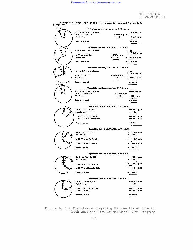
MIL-HDBK-41615 NOVEMBER 1977
Figure 6. 1.2 Examplesboth West
of Computing Hour Angles of Polaris,and East of Meridian, with Diagrams
6-3
Downloaded from http://www.everyspec.com

MIL-HDBK-41615 NOVEMBER 1977
for these observations, since no artificial lighting is required for
illumination of the theodolite cross hairs, and marks at the site can
be easily seen. Very precise azimuth determinations are possible by
this method; even at the most unfavorable time, when Polaris is near
culmination, an error of as much as 1 minute in timing causes a bear-
ing angle error of only O. 3 minute of arc at latitude 40° [96].
6. 1.1.6 Azimuths can be determined by observation of Polaris from
about latitude 10° N to 65° N; for other northern latitudes, and for
locations in the Southern Hemisphere, azimuths may be determined by
reference to other stars or the sun. Star charts and tables for the
reduction of observational data are contained in most ephemerides
[90, 91] and the techniques are discussed in surveying manuals, such
as those referenced in the preceding paragraph.
6. 1.2 Observational procedure
a.
b.
c.
d.
e.
Set watch to exact standard time by monitoring a time
broadcast station.
Set up the theodolite or transit, and carefully level the
instrument.
Set up a mark at a distance of 100 to 200 meters from
the observation station. If observations are planned
for hours of total darkness, provision must be made
for lighting the mark. Center the
mark (0° azimuth).
Focus telescope on a distant light
instrument on the
or star.
Locate Polaris (see figure 6. l-l). Bisect the star, and
note the exact time (if working alone, a s top watch
may be useful). Record the horizontal angle from
the mark to Polaris.
6-4
Downloaded from http://www.everyspec.com

MIL-HDBK-4 1615 NOVEMBER 1977
f.
g.
h.
i.
j.
k.
Reverse the telescope, bisect the star, and record
time and horizontal angle.
With the telescope in the reversed position, again
bisect the star and record time and angle.
Return the telescope to the direct position and make. a
fourth observation.
Use the average watch time of the four observations to
determine the correct local time of the Polaris
observation.
Determine the mean horizontal angle from the mark to
Polaris, and to this apply the azimuth of Polaris at
the mean time of observation to obtain the true bearing
of the reference mark.
Lay off a reference baseline on the site.
6. 1.3 Determination of local mean time
6. 1.3.1 The distinctions between the various time designations are
important. Apparent time is based upon the real sun, with a day
counted from the sun’s meridian passage on one day to the meridian
passage on the next. This rate is irregular. Mean solar time is based
upon an imaginary sun whose day is uniform. This is the time general-
ly used for civil purposes, while sidereal time is used by astronomers.
A sidereal day is equivalent to 23 hours 56 minutes 4.091 seconds in
mean solar time.
6. 1.3.2 Local mean time is identical with mean solar time on the
meridian where that time is employed, and standard time is the same
as mean solar time on the central meridians of each time zone in the
U.S. (e. g. , Eastern ‘Standard Time is based on the 75th meridian
time). Standard time is reckoned from the meridian passing through
the observatory at Greenwich, England (longitude 0°); in this time zone
6-5
Downloaded from http://www.everyspec.com

MIL-HDBK-41615 NOVEMBER 1977
standard time is called Greenwich Civil Time (G CT), Greenwich
Mean Time (GMT), or Universal Time (U. T. ). If we consider the
apparent movement of the sun from east to west in the celestial sphere
(the dome of the sky as viewed from a point on earth) we find that when
the sun crosses the meridian at Greenwich it is noon or 1200 hours
G CT, but it is not yet noon on meridians west of Greenwich, and noon
has already passed at meridians east of Greenwich. Standard or meano
solar time varies by one hour for each 15 of longitude, thus there is
a difference of 5 hours between Greenwich and the 75th meridian in
the U.S. Time zone boundaries are arbitrarily set, frequently to con-
form to political or geographical boundaries, and in some parts of
the world the “official” time does not conform to a standard number of
hours from Greenwich. For example, many countries in Europe which
are in the Greenwich time zone have chosen to use Central European
Time (based on the 15° E meridian) as their official time. Great
caution must therefore be used in converting from the local official
time to local mean time or Greenwich Civil Time.
6. 1.3.3 Tabular data in the ephemeris are listed for mean time
at Greenwich, and calculations related to Polaris observations require
the local mean time at the point of observation. It is usually conven-
ient to use a watch set to standard time and correct the mean time
of observation for the distance east or west of the standard meridian.
Corrections are based upon the following relationships:
6-6
Downloaded from http://www.everyspec.com

MIL-HDBK-41615 NOVEMBER 1977
Longitude (arc) Time
360° 24 hrs
15° 1 hr
1° 4 minutes
15’ 1 minute
1’ 4 seconds
15" 1 second
1" 0.067 second.
Note the distinction between minutes and seconds of arc (longitude)
and minutes and seconds of time. A station east of a standard meridian
will have a later LMT than a station on that meridian, and a station
west of the meridian will have an earlier LMT.
6. 1.3.4 To illustrate the method of converting from standard time
to LMT, consider the following example:
Latitude 40° 30’ 00” N, Longitude 92° 30’ 10” W.
Date: April 20, 1972
Mean watch time of observation: 18 hrs 27 min 55 sec CST.
Since the observation point is 2° 30' 10" west of the time zone meridian
(90° W), the “sun” time or local mean time is somewhat earlier than it
would be if the site were exactly on the 90th meridian. The correction
is as follows:
2° = 8 minutes
30' = 2 minutes10" = .67 seconds (or .01 min. )
Total correction = 10 min 0.67 see, or 10.01 min.
6-7
Downloaded from http://www.everyspec.com

MIL-HDBK-41615 NOVEMBER 1977
Applying this correction, we obtain
18 hr 27 min 55 sec
-10 min 0.67 sec
18 hr 17 min 54 see, or 18 hr 17.91 min Local Mean Time
If our site had been east of the meridian by the same amount (longitude
87° 29’ 50” W) the correction would have been the same, but it would
have been added to the time of observation (CST) to obtain LMT. Also,
if the watch used is known to be fast or slow at the time of observation
this must be taken into account.
6. 1.4 Hour angle determination
6. 1.4.1 After obtaining the LMT of the observation, we can proceed
to the calculation of the hour angle. For the example mentioned above,
we would refer to the table on page 3 of the Bureau of Land Manage-
ment ephemeris [90], and find that on April 20, 1972 the upper culmin-
ation (U.C.) occurs at 12:09.0 p.m. and the declination is 89°08' 20.48".
This time for U. C. is the mean time on the Greenwich Meridian, and
mean time of U.C. on other meridians will be slightly different because
of the difference between solar and sidereal time. Referring to the
table on page 27, for 90° 30’ W longitude the correction is -1 min
01 see; therefore the local mean time of culmination at our observation
point is 12:09.0 - 1.0 = 12:08.0 LMT. Now we draw an hour-angle
diagram:
6-8
Downloaded from http://www.everyspec.com

MIL-HDBK-41615 NOVEMBER 1977
A number
figure 6.1
6.1.5
6.1.5.1
table with
Figure 6.1-3 Example Hour-angle Diagram
of examples of hour-angle computations are given in
-2.
Azimuth of polaris
Referring now to page 19 of the ephemeris, we enter the
the hour angle and the station latitude, and find the azimuth
by interpolation:
Hour Angle 40°
6:09.0 67.1
6:09.9 67.082
6:19.0 66.9
Latitude
40°30'
67.6
To this value we make a correction for declination, obtained from the
right-hand columns of page 19: +0. 2.
The corrected azimuth is 67.8', or 1°07.8'.
If we assume that the mean horizontal angle (mark to star) was
22° 30.1’,
22° 30.1'+1° 07.8'
23° 37.9'
6-9
4 2O
69.2
69.182
69.0
Downloaded from http://www.everyspec.com
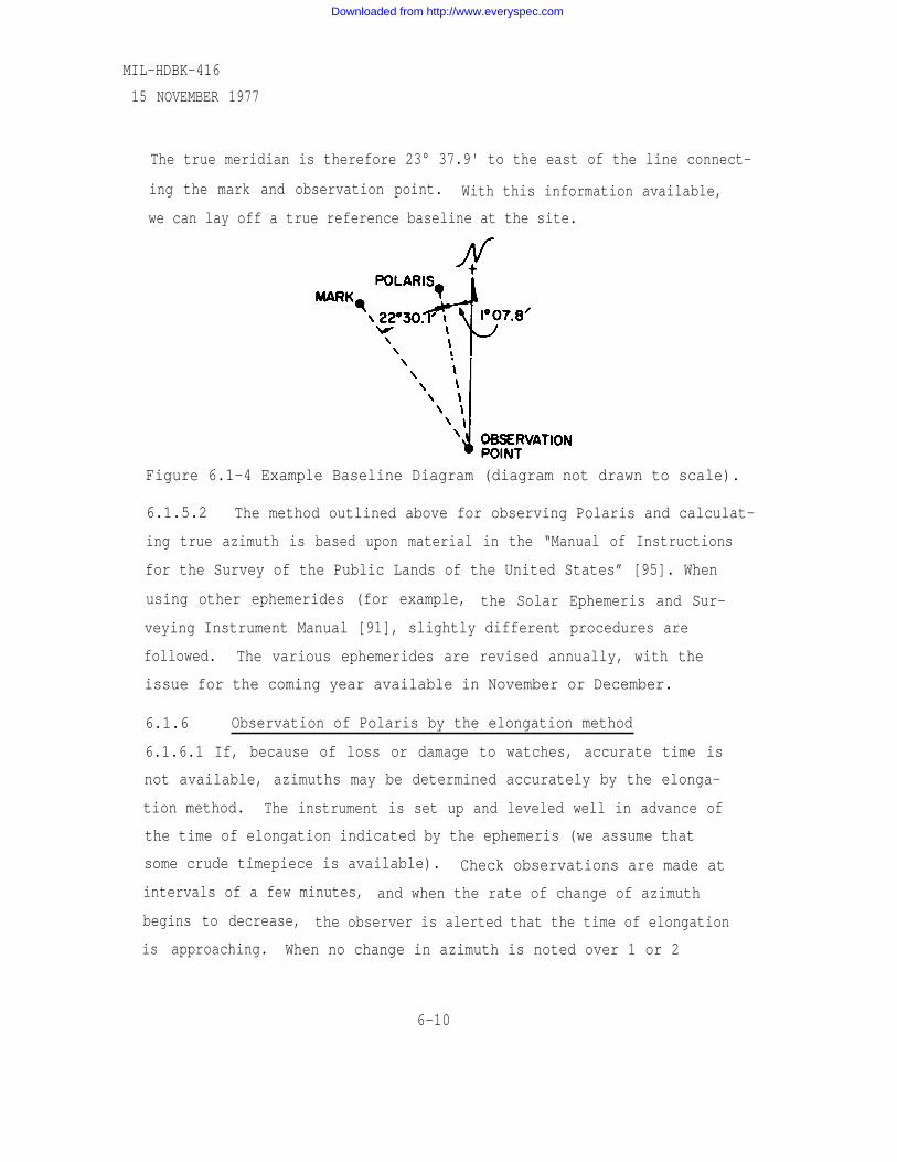
MIL-HDBK-416
15 NOVEMBER 1977
The true meridian is therefore 23° 37.9' to the east of the line connect-
ing the mark and observation point. With this information available,
we can lay off a true reference baseline at the site.
Figure 6.1-4 Example Baseline Diagram (diagram not drawn to scale).
6.1.5.2 The method outlined above for observing Polaris and calculat-
ing true azimuth is based upon material in the “Manual of Instructions
for the Survey of the Public Lands of the United States” [95]. When
using other ephemerides (for example, the Solar Ephemeris and Sur-
veying Instrument Manual [91], slightly different procedures are
followed. The various ephemerides are revised annually, with the
issue for the coming year available in November or December.
6.1.6 Observation of Polaris by the elongation method
6.1.6.1 If, because of loss or damage to watches, accurate time is
not available, azimuths may be determined accurately by the elonga-
tion method. The instrument is set up and leveled well in advance of
the time of elongation indicated by the ephemeris (we assume that
some crude timepiece is available). Check observations are made at
intervals of a few minutes, and when the rate of change of azimuth
begins to decrease, the observer is alerted that the time of elongation
is approaching. When no change in azimuth is noted over 1 or 2
6-10
Downloaded from http://www.everyspec.com

MIL-HDBK-41615 NOVEMBER 1977
minutes (Polaris appears to move along the vertical cross hair) obser-
vations of the indicated azimuth should be started, and continued until
horizontal movement of the star is again evident. observations should
be alternated between direct and reversed position of the telescope;
select a set of four readings that embrace the extreme position of the
star and use the mean of these readings as the azimuth at elongation.
Then enter the table on page 22 of the ephemeris [90] with the station
latitude and determine the star to pole azimuth at the time of elongation.
Then calculate the true bearing (mark to pole) as in the hour-angle
method.
6.1.6.2 There is a period of about 15 minutes on either side of the
point of elongation when the azimuthal change is only about 1' of arc,
so nearly continuous observation during this period is recommended.
6.1.7 Checking of azimuth
6.1.7.1 It is recommended that the calculations for azimuth from the
observational data be made independently by two members of the sur-
vey party.
6-11
Downloaded from http://www.everyspec.com

MIL-HDBK-41615 NOVEMBER 1977
Section 6.2 DETERMINATION OF ELEVATION BY ALTIMETER SURVEYS.
6.2.1 Altimeters are essentially aneroid barometers calibrated to
indicate altitude instead of pressure. The pressure-height relation-
ship is based upon an assumed “standard” atmosphere; these so-called
standard conditions will seldom, if ever, be found in the real atmos-
phere, so that some error is nearly always present. A commonly
used relationship for scale calibration of surveying altimeters is
based upon the assumption of a completely dry, isothermal atmos-
phere with a uniform temperature of 10° C (50° F) and a sea-level
pressure of 29.90 inches of mercury [92]. Since the sea-level pres-
sure sometimes exceeds this value, an altimeter calibrated on this
assumption will sometimes show negative values of altitude; this is
avoided on other instruments by placing the scale zero at -1000 ft
(pressure 31.026 inches) so that readings will always be positive.
With the latter scale calibration, however, the indicated altitude is
usually about 1000 ft higher than the true altitude.
6.2.2 Pressure always decreases with altitude, roughly at the
rate of about one inch per 1000 ft; thus at 5000 ft above sea level the
actual atmospheric pressure will be around 25 inches
Barometers (and altimeters) indicate the total weight
point of observation; this varies with the temperature
of mercury.
of air above the
and humidity of
the air masses and is greatly influenced by moving weather systems.
Altimeter surveys should be conducted only during stable weather con-
ditions, when winds are light and the pressure and temperature are
reasonably steady over the survey area; operations should be suspended
in stormy weather or when winds are high or gusty.
6.2.3 In spite of the limitations outlined above, the surveying
altimeter is very useful for determining differences in elevation
6-12
Downloaded from http://www.everyspec.com

MIL-HDBK-41615 NOVEMBER 1977
between two points, one of which is a benchmark or other location of
known elevation. By making corrections for temperature and humidity
differences (which affect the density of the air), horizontal and temporal
changes in pressure, and scale calibration temperature, very rapid
and accurate surveys can be obtained. It should be noted that the
“scale calibration” correction is completely separate from the air
temperature correction; the scale is engraved under laboratory condi-
tions with a temperature of about 24° C (75° F), and when used in the
field under different temperature conditions a slight scale change
occurs.
6.2.4 The following general precautions are applicable to most
surveying altimeters:
a. Handle the instrument as you would a good watch -- do
not drop or jolt it, and pack in a padded case when
shipping or moving in a vehicle.
b. Never expose the altimeter to the direct rays of the
sun -- use in the shade, or shield with the body during
observations. Avoid placing the instrument on hot
pavement, rocks, metal roofs, etc.
c. Always read the instrument in the same position
(normally horizontal) and be careful to avoid parallax
errors -- if the dial has a reflector ring, make the
reading when the pointer and its image appear coinci-
dent.
d. If there is a large change in temperature between two
observation points, allow a period of time before the
second reading to permit the instrument to reach
thermal equilibrium.
6-13
Downloaded from http://www.everyspec.com

MIL-HDBK-41615 NOVEMBER 1977
e. Tap the case of the altimeter lightly with a finger or
pencil eraser before reading; this helps reduce errors
caused by mechanical lag or friction in the mechanism.
f. When several altimeters are used by a field party, it
is a good practice to make comparative readings at
least once each day and record the values in the field
notebook. Any large change in the differences between
instruments is reason to suspect possible instrument
damage.
g. Avoid frequent resetting of the dial pointers in the
field. It is better to make corrections to field readings
based upon the most recent benchmark-to-altimeter
comparison.
h. After checking an altimeter at a benchmark, observa-
tions at the various points in the field should be made
as quickly as possible. Even when the general pres-
sure systems are static there are regular diurnal
variations that must be allowed for -- a sort of atmos-
pheric tide. These diurnal variations have a 12-hour
period and cause maxima at 1000 and 2200 local time,
and minima at 0400 and 1600 [94]. In the tropics these
are the most important pressure fluctuations and are
very regular from day to day; in temperate and higher
latitudes the diurnal effect is frequent masked by the
larger pressure changes caused by moving pressure
systems, but the “tidal” effect is still present.
6.2.5 There are a number of ways in which altimeter surveys can
be conducted; the choice depends largely upon the personnel and num-
ber of instruments available, as well as the accuracy required from
6-14
Downloaded from http://www.everyspec.com
MIL-HDBK-41615 NOVEMBER 1977
the particular survey. Two procedures will be described, the single-
base method and the two-base method [93, 96].
6.2.6 In the single-base survey, two altimeters are required. One
remains at a benchmark or other point of known elevation, with read-
ings of the altimeter made at regular intervals -- say every 5 or 10
minutes. The other instrument, referred to as the roving altimeter,
is read at the various points along the path where elevations are desired.
At both stations, temperature and humidity measurements are obtained
with small battery-powered psychrometers, or with the sling-type
psychrometers packed in the case of many surveying altimeters. The
indicated differences in elevation are corrected by a factor determined
by the mean temperature and humidity over the path from benchmark to
field point at the time of the field observation; tables or nomograms for
the corrections are included with the altimeters. The corrected dif-
ference in elevation is then combined with the known elevation of the
base station or benchmark to obtain the desired elevation field point.
(Corrections may also be required for the scale temperature).
6.2.7 The two-base method. eliminates the need for temperature
and humidity corrections, although the temperature must still be
checked to determine if scale temperature corrections are necessary.
One station is established at a low point in the area, and a second
station at a high point; the points of unknown elevation are between
these two stations. The elevations of the base stations must be known;
if possible they should be located at benchmarks. A third altimeter is
carried to the field sites where elevations are desired. All three
altimeters are read simultaneously, either by prearranged schedule
or by radio coordination. It is assumed that the atmospheric proper-
ties change linearly between the base stations at a given time, and
that the ratio between the known base-station elevation difference and
6-15
Downloaded from http://www.everyspec.com

MIL-HDBK-41615 NOVEMBER 1977
the altimeter-indicated difference is equal to the ratio between the un-
known elevation difference from base station to field point and the dif-
ference indicated by simultaneous altimeter readings. For example,
Upper base - Lower base (Elevation) = Field Pt. - Lower base (Elevation)Upper base - Lower base (Altimeter) Field Pt. - Lower base (Altimeter)
Use of a computation sheet, such as that shown in figure 6.2-1, is
recommended. The average error of elevations obtained with the two-
base method is said to be 3 ft with the two base stations separated by
10 miles horizontally and 1000 ft vertically.
6.2.8 There will be occasions when limitations of personnel or
equipment may require a single-altimeter survey. In this case, take a
reading at a benchmark. If the two benchmark altimeter readings vary
by more than a few feet, repeat the sequence; in any case, it is prefer-
able to take a series of readings and use the average elevation difference
in determining the elevation of the field point.
6.2.9 There are recording altimeters available which reduce the
manpower demands of the single-or two-base surveys. A recording
micro barograph is also very useful on a field survey to obtain a con-
tinuous record of the pressure variations related to diurnal effects or
moving pressure systems; with the aid of this record one can elimin -
ate or recheck observations made during periods of rapidly changing
pressure, or even correct field observations for the dynamic pressure
component.
6-16
Downloaded from http://www.everyspec.com

MIL-HDBK-41615 NOVEMBER 1977
Observer J. Porter
Date 10 Sept. 71
(1) Upper Base Station Elevation 1000 (Location) B. M. 2-Longhill
(2) Lower Base Station Elevation 400 (Location) Airport Runway 6
(3) Difference (1 - 2) 600
(4)
(5)
(6)
Altimeter Reading, Upper
Altimeter Reading, Lower
Difference (4 - 5)
Base
Base
1200
500
700
(7) Altimeter Reading; Field Site
(8) Altimeter Reading; Lower Base
(9) Difference (7 - 8)
(10)
(11)
(12)
(13)
Divide (3/6)
Multiply (10 x 9)
Elevation; Lower Base (2)
Elevation; Field Site (11+12)
Site # A
800 570
0.857 0.857 0.857
257.10 59.99
400 400 400
657 460
Figure 6.2-1 Two-base Altimeter Survey Computations
6-17
Site # B Site # C
500 500
300 70
500
Downloaded from http://www.everyspec.com
MIL-HDBK-41615 NOVEMBER 1977
6.2.10 The effect of these dynamic pressure changes on survey
accuracy can be significant, as shown by the following example:
Between 1000 and 1200 local time, while an altimeter survey was in
progress, the barograph shows a pressure fall of 0.10 inches.
(Changes of this magnitude occur frequently in many parts of the
world.) Using the rule-of-thumb relationship that a change in eleva-
tion of 1000 ft results in a pressure change of about one inch of mer-
cury, a change of 0.10 inch is equivalent to an elevation difference of
about 100 ft. Therefore during the 2-hour period while the survey was
in progress, the dynamic pressure component was causing the equiva-
lent of a 25-ft elevation difference (at a point) each 30 min.
6.2.11 Another source of altimetry error is related to the horizontal
gradient of pressure, which is indicated by the spacing of isobars on
weather maps. A survey proceeding on a line perpendicular to the
isobars in the vicinity of a moderately intense storm system might
incur errors on the order of 1 to 3 ft per mile, related to this hori-
zontal difference in the pressure field. Under such circumstances,
however, the surface winds could be expected to be 15 mph or more,
and if the rule mentioned previously of taking surveys only during
very light wind conditions is followed, the horizontal pressure gradient
error should be relatively minor.
6-18
Downloaded from http://www.everyspec.com

MIL-HDBK-41615 NOVEMBER 1977
Section 6.3 OPTICAL METHODS OF CHECKING RADION-PATH OBSTRUCTIONS.
6.3.1 Introduction
6.3.1.1 Obstruction clearance, location, and elevation can be calcu-
lated from observations of lights on a tower at one end of a line-of-
sight path from the other end. Binoculars are often useful for making
these observations. The lights used may be sun reflection flashes,
xenon tube flashes, a laser beam, or an ordinary high-intensity electric
lamp. All of these sources have advantages, but the xenon flash tube
seems to be the most convenient source with a long range. The flashes
have the additional advantage of being easily identifiable. Xenon
flashes with an effective radiated peak power of a million or more watts,
can be obtained from portable equipment.
Light-ray bending through the atmosphere is about the same
as for radio waves in a well-mixed atmosphere, and errors in deter-
mining radio clearance from optical measurements should not be
appreciable on the normal line-of-sight paths under such conditions.
On the tower at F in figure 6.3-1, a light is located at a
potential upper antenna position, D, with another light below it at B.
The location of B is not critical but it must be compatible with the
height of the tower at E. Also for a path with two predominate obsta-
cles care must be taken in choosing the heights of B and C. The height
of D and B above ground must be measured. The ground elevations
above mean sea level, m.s.1., of sites E and F should be known as
well as the distance, d, between E and F. At site E the height above
ground where light D is half obstructed from view (C) is measured,
also the height A where B is half obstructed.
Using the standard slope-intercept formula for a straight
line, y = mx + b, the intersection of lines AB and CD at the obstacle
6-19
Downloaded from http://www.everyspec.com

Figure 6.3-1
MIL-HDBK-41615 NOVEMBER 1977
6-20
Downloaded from http://www.everyspec.com

MIL-HDBK-41615 NOVEMBER 1977
(xO, yO) can be readily calculated. The difference between the value
of y on the line at xO and the value of yO is the clearance over the
obstacle for the meteorological conditions prevailing at the time when
the observation of the light at D and B was made. The value, d1 = xO,
should be verified using the map profile if one is available.
Using the configuration in figure 6.3-1 as an example, the
distance to the obstacle, d1; the clearance, and the height of the
obstacle above m.s.1., hO, is calculated as
From the tower coordinates at E and F, the
20 km. The elevation above m.s.1. at E is
D was determined to be 35 m above F and B
observed to be 41 m above E and C was 3 m
follows :
distance, d is found to be
1100 m and at F it is 21 m.
was 7 m above F. A was
above E.
The coordinates of A, B, C, and D are as follows:
or
(xA, yA)
(xB, yB)
(xC, yC)
(xD, yD)
For y = -0.05565 x + 1141
For y = -0.05235 x + 1103
For y = -0.05425 x + 1141
(0, 1141)
(20000, 28)
(0, 1103)
(20000, 56).
(6.3-1)
(6.3-2
(6.3-3)
(6.3-1)
(6.3-2)
(6.3-3)
6-21
=
=
=
=
Downloaded from http://www.everyspec.com

MIL-HDBK-41615 NOVEMBER 1977
Subtracting eq. 6.3-2 from eq. 6.3-1,
0.0033 xO = 38
d1 = xO = 11,515.1 m
yO = 500.2 m
For
y = -624.69 + 1141
y = 516.31 m.
Then = 516.31 - 500.2 = 16.1 m.For m.s.1. at xO assuming k=4/3, from figure 6.3-1 and paragraph 4.2.15.2
Substituting for the example,
Then ho = 500.2 -5.6 =494.6 m. Note that six place accuracy should
be used in some of these calculations.
Methods for determining clearance by measuring elevation
angles from the obstruction itself are available but these methods have
the disadvantage that it is often difficult to orient yourself in the area
where the obstacle is located and many times the obstacle is relatively
inaccessible.
6-22
at xO,
Downloaded from http://www.everyspec.com

MIL-HDBK-41615 NOVEMBER 1977
Section 6.4 EQUIPMENT, TOWERS, CALIBRATIONS, AND TEST PROCEDURES FORPATH LOSS MEASUREMENTS .
6.4.1 Introduction
6.4.1.1 Path-testing of a radio route is a large and expensive opera-
tion, which must be carefully organized and well run to get the best
results. Temporary test-towers must be set up at each proposed
repeater site, with the radio transmitter at one end of a path and the
receiver at the other. Height-loss curves are obtained for each path
and analyzed before moving to the next path. The transmitter T and
receiver R leap-frog along the route, and while one path is being tested,
the construction crew erects the next test tower. The requirements
for equipment, towers, crew, etc., are discussed
below.
6.4.2 Characteristics of the radio equipment
6.4.2.1 The main requirements of a test system
testing are accuracy, reliability, portability, weatherproof operation,
and ease and convenience of operation. It must also be packaged for
in more detail
to be used for path-
mounting on an antenna carriage) and so must be lightweight. For
extra convenience and ease of operation, the power and control units of
the microwave equipment are often mounted in trucks with specially
built bodies. They can then be removed easily for testing from roof
tops or inaccessible locations.
6.4.3 Typical test link
6.4.3.1 There are several different types of equipment available,
operating in the 4 and 8 GHz bands. The transmitter and receiver are
packaged in weather proof units mounted on the rear of parabolic dish
antennas. These antennas ride up and down the tower on antenna
carriages, which run on tracks attached to the tower, or on the tower
6-23
Downloaded from http://www.everyspec.com

MIL-HDBK-41615 NOVEMBER 1977
members themselves. Provision is made for tuning the test equipment
over the desired frequency range, and to monitor frequency and output
power. The test equipment may be powered by either battery or a.c.,
and all power and control voltages are carried up a control cable, to
the radio-frequency units, from a control cabinet at the base of the
tower. When used for path-testing, the receiver is calibrated in deci-
bels from free-space loss, or power measured at the receiver input
terminals, sometimes by means of operating from the receiver auto-
matic gain control or an IF log-linear amplifier. The signal level is
then obtained directly from the meter reading, using a calibration
curve.
6.4.4 Test-towers
6.4.4.1 Before deciding on the
sary to determine what height of
type of test-tower
tower is required.
bearing not only on the cost of the path-testing, but
to use, it is neces-
This has a direct
on the results
obtainable. On 4 and 6 GHz routes, where the average path length is
roughly 40 km, permanent towers up to 100 m are common, and longer
paths or higher towers occur frequently. Figure 6.4-1 shows a typical
48.3 km path, with the profile plotted for k = 4/3. The two obstructions
are also plotted for k = 2/3, plus the usual clearance for the
first Fresnel-zone radius.
6.4.4.2 The heights of the tower required to give this clearance at
k = 2/3 are roughly 60 m at each end, as shown. However, the area
between 18 and 37 km contains potential reflecting surfaces. It is
therefore desirable to search for reflections with path clearances
equivalent to those occurring when k approaches infinity. The earth
bulge at midpath is roughly 34 m at k = 4/3 versus zero at k =
Hence, a test-tower 100 m high at both ends of the path is required.
6-24
Downloaded from http://www.everyspec.com

MIL-HDBK-41615 NOVEMBER 1977
Figure 6.4-1 Required Height of Test-tower.
Experience shows that it very seldom pays to use less than 60 m. A
good rule is to estimate the tower height required to measure two even
zones from possible reflecting surfaces in the path. This usually
means towers 100 m high.
6.4.4.3 One type of tower often used is erected from the bottom up,
by inserting the next section. The sections come in either square or
triangular cross -section as shown in figure 6.4-2. The sections are
made of tubular metal, usually aluminum, and the corners form tracks
up which the antenna carriage runs. Erection of the tower requires a
crew of about 12 men and 4 to 8 hours of working time.
6.4.4.4 Another type of tower often used is a scaffolding type, avail-
able in heights up to 100 m or more. It is a guyed tower, built in sec-
tions which fold up for shipping. To erect the tower, the sections are
stacked one on top of the other, being hoisted to the top with a ginpole
arrangement before being bolted in place. Each 2 m section includes
a platform, and stairs which zigzag up inside the tower. This makes
it easy to do optical tests and to adjust the equipment. Special tracks
which hook to all four sides of the tower permit the use of deep wheel
flanges, thereby eliminating danger of the carriage coming off the
tracks, see figure 6.4-2c.
6-25
Downloaded from http://www.everyspec.com
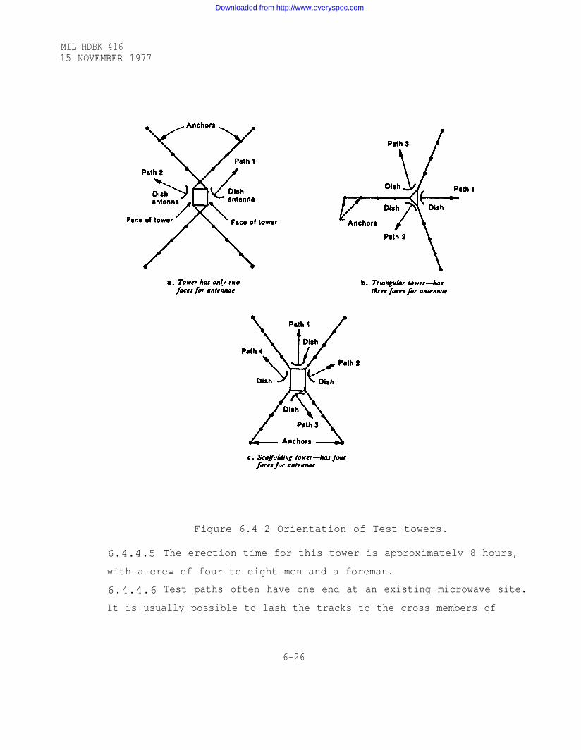
MIL-HDBK-41615 NOVEMBER 1977
Figure 6.4-2 Orientation of Test-towers.
6.4.4.5 The erection time for this tower is approximately 8 hours,
with a crew of four to eight men and a foreman.
6.4.4.6 Test paths often have one end at an existing microwave site.
It is usually possible to lash the tracks to the cross members of
6-26
Downloaded from http://www.everyspec.com

MIL-HDBK-41615 NOVEMBER 1977
the permanent tower. The special tracks of the scaffolding type tower
can be used in the same way (they may require extra cross pieces
mounted temporarily on the existing tower).
6.4.4.7 The tower shown in figure 6.4.2a gives a coverage us-
ing two antenna carriages on opposite faces of the tower. However,
because the path bearings are seldom 180° apart, it is often difficult to
orient the tower correctly. Local conditions may limit the choice of
suitable anchor locations and correct orientation of the tower must be
decided on the spot. This is not a problem with the triangular tower
(three faces) or the scaffolding tower (four faces). Path bearings
should be marked with stakes. Anchor locations should also be staked.
6.4.4.8 The test-tower must be erected on the same spot as the
permanent tower, so the proper spot must be agreed on before testing
begins. The test site should be marked by iron stakes, and a plot plan
should show measurements to prominent features of the terrain. The
exact location will then not be lost if the stakes are disturbed. If
these precautions are not taken, the permanent tower may easily be
located to one side of the test path, resulting in extra obstruction
height and a poor or unworkable path. The time and money spent on
path-testing can be completely wasted if these precautions are not
taken.
6.4.4.9 A second precaution must be taken, i.e., allowance must be
made for changes in elevation of the site during construction. Grading
or filling of the site often changes the grade level by many meters.
6.4.4.10 These changes must be allowed for when specifying antenna
heights. Antenna elevations should be given, not tower heights. They
can be quoted relative to an arbitrary datum set up on the site, to
make sure the tower provides the correct antenna heights.
6-27
Downloaded from http://www.everyspec.com

MIL-HDBK-41615 NOVEMBER 1977
6.4.5 Associated test equipment
6.4.5.1 The test equipment
quired, depending on the type
a.
b.
c.
d.
e.
f.
g.
h.
i.
j.
k.
power meterfrequencies;
listed below is typical of what may be re-
of radio equipment used for testing:
- to measure power levels at radio
signal generators - to generate radio-frequency signals;
waveguide and coaxial attenuators - to adjust radio-frequency power levels;
waveguide to coaxial transitions;
log-linear amplifiers;
microwave receiver (solid state);
preselector filter;
microwave antennas;
directional couplers;
signal-level recorders;
a VHF radio-link is used for talking between trans-mitter and receiver sites. Antennas for this systemare usually ground-plane types, mounted on top of thetest tower. Yagi or corner-reflection types are alsoused if extra gain is needed, or interference is aproblem.
6.4.6 Antenna carriage
6.4.6.1 The antenna carriage is a light metal framework,
ride up and down the tower carrying the test antenna and the
designed to
transmitter
or receiver. It should have motors to adjust azimuth
the antenna by remote-control from the ground. This
the need for manpower at the test site, and increases
racy in making tests.
6.4.6.2 The antenna carriage is raised and lowered
and elevation of
greatly reduces
speed and accu-
by means of a
winch. The winch fits on the tower and can be hand-powered or motor-
driven. Any motor-driven winch used should be arranged to stall well
6-28
Downloaded from http://www.everyspec.com

MIL-HDBK-41615 NOVEMBER 1977
before the breaking point of the cable is reached. A safety cut-off
switch should be mounted on the carriage, with a suitable stop installed
at the tower top. A counter weight may be helpful for hand operated
height variable equipment.
6.4.7 Power requirements
6.4.7.1 The radio test equipment may be powered either by a.c. or
battery, but there is sometimes a need for a.c. to charge batteries,
and to operate winches, azimuth and elevation motors, radio communi-
cation equipment, tower lights, test equipment, etc. In choosing a
power source, it should be noted that:
a. at high altitudes, engines often become less efficient,output drops and voltage regulation suffers, so a largecapacity is needed;
b. good frequency and voltage regulation are essential.Generators must be located far enough away thatnoise is not a problem; the long power feeds thencause a large voltage drop;
c. accurate test results depend on well-regulated linevoltage at both transmitter and receiver;
d. continuous-duty rating is required. The radio equip-ment should normally be left on to reduce surges andwarm-up time, and prevent condensation of moisturein the equipment.
6.4.8 Licensing of radio equipment
6.4.8.1 A radio-station license is usually needed for the radio test
link and the VHF radio communication link.
6.4.8.2 Approval of government agencies is necessary for each test
tower erected. Data must be provided on dates of erection and dis-
mantling of each tower, ground elevation, tower height, and latitude
and longitude. Alternative sites should be approved in advance, to
avoid delay in case test paths prove unsatisfactory. Licensing
6-29
Downloaded from http://www.everyspec.com

MIL-HDBK-41615 NOVEMBER 1977
agencies often require painting and lighting of all towers, or those
exceeding a certain elevation.
6.4.8.3 Details on local requirements should be checked with the
national or other government agencies concerned.
6.4.9 Manpower requirements
6.4.9.1 Nominal requirements are one engineer, one technician and
two others.
6.4.10 Calibrations:
6.4.10.1 The test receiver should be calibrated before starting tests
each day and checked at intervals, as required. The transmitter out-
put should be measured and checked periodically. Some of the small
solid-state microwave oscillators are very stable in power output.
6.4.11 Radio-frequency levels in a radio path
6.4.11.1 Figure 6.4-3 illustrates the variation in level of the radio-
frequency signal over a typical microwave path. The free-space path
loss is actually the loss between antennas, but the calibration technique
must simulate the
technique of doing
ing at a frequency
signal arriving at the receiver converter. The
this is described below, for a typical test link operat-
of 4 GHz.
Figure 6.4-3 Levels of the Radio-frequency in a Radio
6-30
Path.
Downloaded from http://www.everyspec.com

MIL-HDBK-41615 NOVEMBER 1977
6.4.12 Typical calibration procedure
6.4.12.1 The equipment should be allowed to warm up for stable opera-
tion (a minimum of 30 min). The transmitter is then tuned to the de-
sired test frequency, the output is measured and recorded in the log
book.
6.4.12.2 The receiver should be carefully aligned and tuned to the test
frequency. The free-space path loss is then calculated for that fre-
quency, for the particular path length. The theoretical free-space input
signal at the receiver can then be calculated by subtracting the sum of
antenna gains and transmitter output from the free-space loss. This is
the level at the point X in figure 6.4-3, and is the level that must be
simulated by the calibration procedure.
6.4.12.3 Figure 6.4-4 is a block diagram illustrating how the auto-
matic gain-control meter of the receiver is calibrated to read the radio-
frequency signal strength. Either a log-linear IF amplifier or automatic
gain control voltage may be used to drive the recorders. The signal-
strength recorder should be connected and calibrated at the same time
as the signal-level meter.
Figure 6.4-4 Block Diagram of the Method of Calibrating theAutomatic-gain-control Meter.
6-31
Downloaded from http://www.everyspec.com
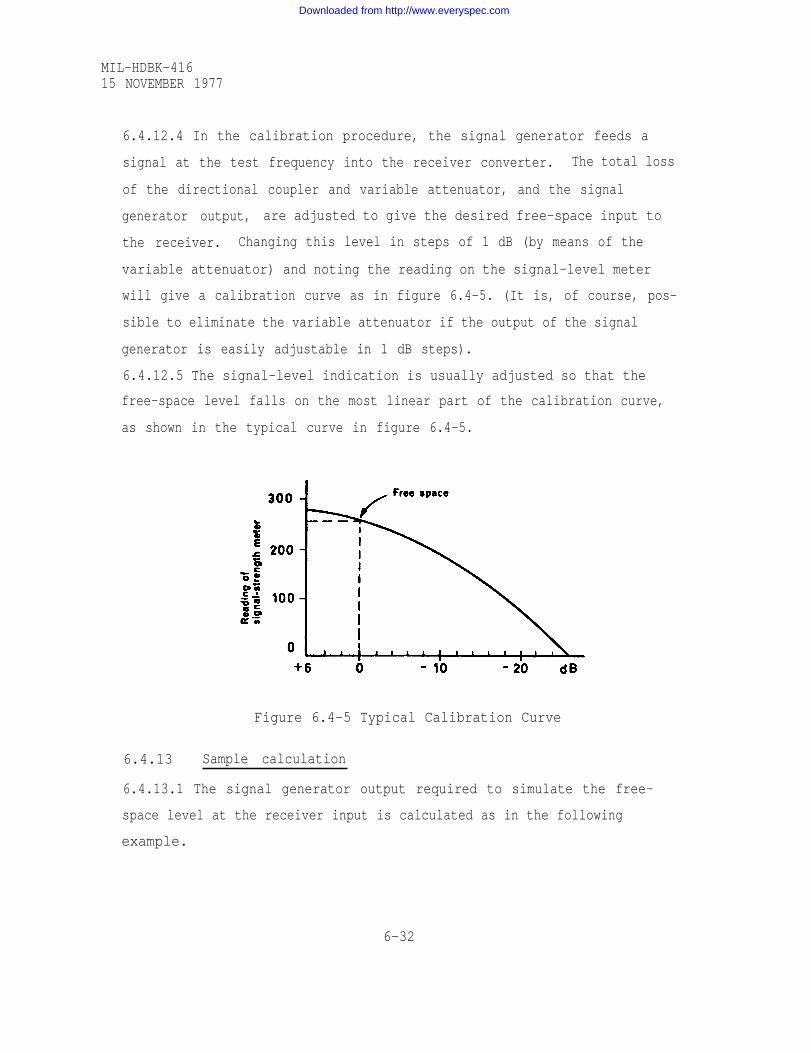
MIL-HDBK-41615 NOVEMBER 1977
6.4.12.4 In the calibration procedure, the signal generator feeds a
signal at the test frequency into the receiver converter. The total loss
of the directional coupler and variable attenuator, and the signal
generator output, are adjusted to give the desired free-space input to
the receiver. Changing this level in steps of 1 dB (by means of the
variable attenuator) and noting the reading on the signal-level meter
will give a calibration curve as in figure 6.4-5. (It is, of course, pos-
sible to eliminate the variable attenuator if the output of the signal
generator is easily adjustable in 1 dB steps).
6.4.12.5 The signal-level indication is usually adjusted so that the
free-space level falls on the most linear part of the calibration curve,
as shown in the typical curve in figure 6.4-5.
Figure 6.4-5 Typical Calibration Curve
6.4.13 Sample calculation
6.4.13.1 The signal generator output required to simulate the free-
space level at the receiver input is calculated as in the following
example.
6-32
Downloaded from http://www.everyspec.com
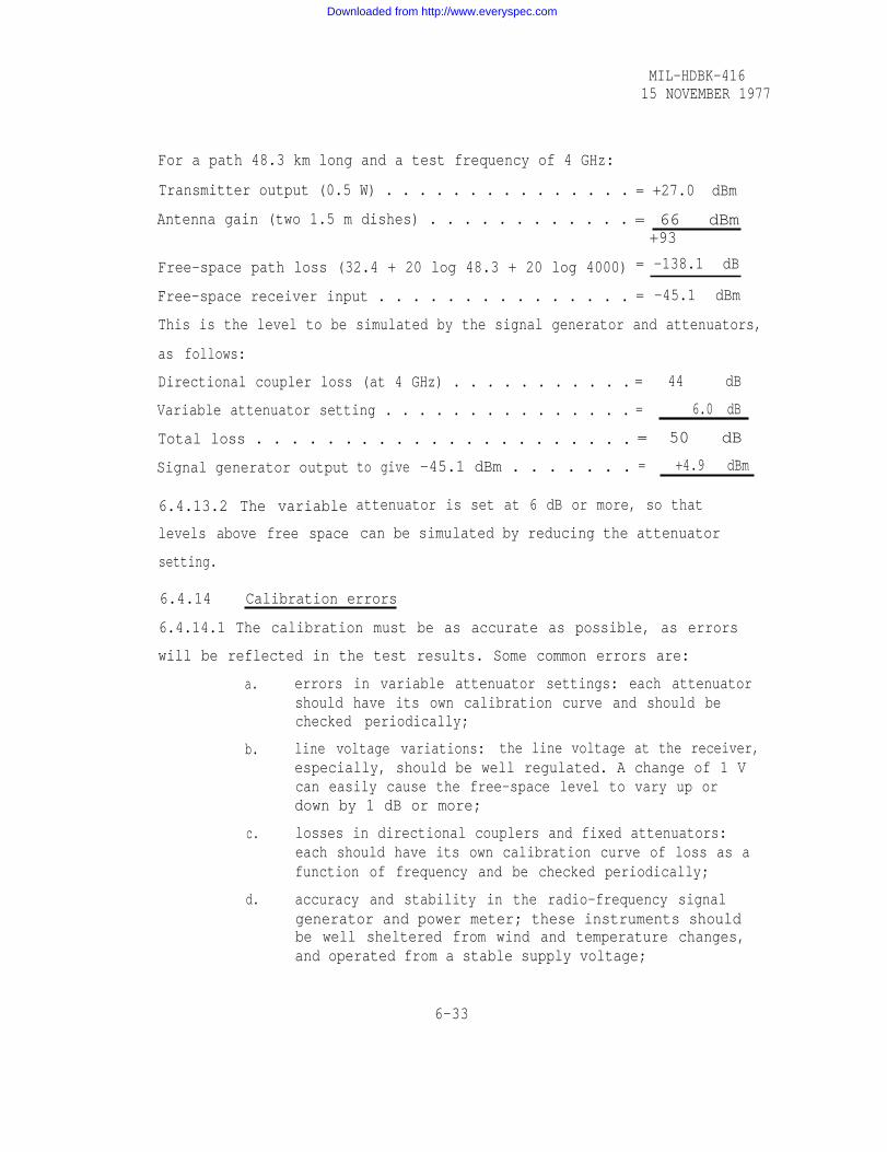
MIL-HDBK-41615 NOVEMBER 1977
For a path 48.3 km long and a test frequency of 4 GHz:
Transmitter output (0.5 W) . . . . . . . . . . . . . . .
Antenna gain (two 1.5 m dishes) . . . . . . . . . . . . = 66 dBm+93
Free-space path loss (32.4 + 20 log 48.3 + 20 log 4000)
Free-space receiver input . . . . . . . . . . . . . . . = -45.1 dBm
This is the level to be simulated by the signal generator and attenuators,
as follows:
Directional coupler loss (at 4 GHz) . . . . . . . . . . .
Variable attenuator setting . . . . . . . . . . . . . . . = 6.0 dB
Total loss . . . . . .
Signal generator output
6.4.13.2 The variable
levels above free space
. . . . . . . . . . . . . . . . = 50 dB
to give -45.1 dBm . . . . . . . = +4.9 dBm
attenuator is set at 6 dB or more, so that
can be simulated by reducing the attenuator
setting.
6.4.14 Calibration errors
6.4.14.1 The calibration must be as accurate as possible, as errors
will be reflected in the test results. Some common errors are:
a.
b.
c.
d.
errors in variable attenuator settings: each attenuatorshould have its own calibration curve and should bechecked periodically;
line voltage variations: the line voltage at the receiver,especially, should be well regulated. A change of 1 Vcan easily cause the free-space level to vary up ordown by 1 dB or more;
losses in directional couplers and fixed attenuators:each should have its own calibration curve of loss as afunction of frequency and be checked periodically;
accuracy and stability in the radio-frequency signalgenerator and power meter; these instruments shouldbe well sheltered from wind and temperature changes,and operated from a stable supply voltage;
6-33
= +27.0 dBm
= -138.1 dB
= 44 dB
Downloaded from http://www.everyspec.com

MIL-HDBK-41615 NOVEMBER 1977
6.4.15
6.4.15.1
6.4.15.2
e.
f.
equipment troubles: the microwave equipment must bein good condition and operated by trained personnel;
antenna pointing: the full gain of the antennas (thevalue used in calculations) must be realized.
Suggested test procedure:
Height-loss tests:
a. Transmitter antenna fixed at one height and the receiverraised or lowered in steps.
b. Receiver antenna fixed and transmitter antenna variedin steps.
All runs should be numbered in sequence; this helps to
identify changes in k, or in calibration of the equipment.
6.4.15.3 The transmitter antenna is oriented on instructions from the
receiver operator, using the VHF radio for communication. The anten-
na heights and signal levels are recorded and immediately plotted. The
antennas are usually raised in steps of 0.5 m and oriented for maximum
signal at each step; the highest reading obtained at each setting is the
one recorded. It is very important to locate all points at which the
height-loss curve reaches the free-space level,
6.4.16 Suggested sequence of tests
6.4.16.1 Upon completion of the first run, the
be examined, in conjunction with the profile, to
maxima, and minima.
height-loss curve should
determine what the
next run should be. Each test should be done twice to insure repeata-
bility. The test sequence should minimize unnecessary movement, and
the tests should be designed to obtain as much information with as few
tests as possible. The tests should be performed by, or supervised
by, an experienced man, to ensure best results. The test sequence
below is intended only as a guide; the results of one test will suggest
subsequent tests designed to get the desired information. One test can
6-34
Downloaded from http://www.everyspec.com

MIL-HDBK-41615 NOVEMBER 1977
often be set up to give data on both obstructions and reflections, there-
by reducing the number of tests needed. Make sure of having one a and
one b run with fixed antenna heights at, or close to, the proposed final
heights. Repeat certain runs during the day, as a check on k and on
calibration. If tests run two days, repeat at least one run from day to
day. Repeat those tests which best define an obstruction or reflecting
surface near the middle of the path, where changes in k will show up
the most.
6.4.17 Worst combinations of antenna heights
6.4.17.1 Once a reflection has been located, the effect of different
combinations of antenna height should be investigated. This is done by
lowering one antenna and raising the other, to maintain the same path
clearance. There are two reasons for doing this:
a. it may be possible to find a range of antenna heightsfor which the reflections are less severe;
b. it is usually possible to locate one combination forwhich the reflection is much more severe. This alsogives a better indication of the true reflection coeffi-cient, and indicates the worst condition to be expectedwhen the path becomes part of a working system.
6.4.18 Test frequency
6.4.18.1 It is usually better to use a test frequency in the same band
as the proposed communications link. It is also possible to test a path
at, say, 6 GHz, when it is intended to operate the link at 4 GHz. Proper
allowance must be made for antenna patterns when analyzing test results,
and to allow the proper clearance at the working frequency.
6.4.19 Signal-level recording
6.4.19.1 It may be desirable to obtain recordings of signal-level
variations on the test paths. These are far from conclusive but do
6-35
Downloaded from http://www.everyspec.com

MIL-HDBK-41615 NOVEMBER 1977
give some indication of propagation conditions over the paths. On
difficult paths, it may also be desirable to obtain long-term records
of fading.
6-36
Downloaded from http://www.everyspec.com
MIL-HDBK-41615 NOVEMBER 1977
section 6.5 PATH LOSS CALCULATIONS FOR SINGLE KNIFE EDGE DIFFRACTION LINES.
6.5.1 Introduction.
6.5.1.1 Although the primary objective of this handbook is to
provide engineering guidelines for the design of microwave line-
of-sight communication links, information relating to performance
estimates for obstructed links is occasionally required when
terrain obstacles blocking the line of sight cannot be avoided by
relocating terminal or relay sites. In most cases of interest to
the microwave system designer the obstruction can be represented
by a single knife edge (ideally, an infinite half-plane). The
methods and procedures in Section 6.5 for long-term median
transmission loss calculations are generally
operating at frequencies above approximately
100 km long. Problems involving diffraction
applicable to links
5 GHz and up to
over smooth earth
or over irregular terrain not representable by a knife edge are
treated in MIL-HDBK-417 on transhorizon microwave system design.
MIL-HDBK-417 should also be consulted for knife-edge diffraction
calculations at frequencies below 5 GHz, and for long-term
transmission loss variability estimates for paths longer than 50 km.
6.5.1.2 MIL-HDBK-417 includes detailed discussion of
diffraction mechanisms, derivation of the equations used, and
extensive references. For the purposes of the line-of-sight
system designer who encounters an obstructed link only
occasionally, it will suffice to provide the required formulas
and graphs in terms of step-by-step procedures. The user is
referred to MIL-HDBK-417 for detailed explanations, references,
6-37
Downloaded from http://www.everyspec.com

MIL-HDBK-41615 NOVEMBER 1977
and other background material. References to appropriate
sections or paragraphs in MIL-HDBK-417 will be provided in
addition to cross references to material in the earlier chapters
of this handbook.
6.5.1.3 Section 6.5 includes determination of applicable
atmospheric and terrain parameters (sections 6.5.2 and 6.5.3) ,
diffraction attenuation calculations for an ideal isolated knife
edge without ground reflections (section 6.5.4), effects of
qround reflections (section 6.5.5) , and effects of rounding of
the knife edge on the attenuation (section 6.5.6).
A brief discussion of fading and long-term variability will
be included as section 6.5.7.
6.5.1.4 Effects of power fading due to diffraction over the
earth's surface when insufficient path clearance exists because
of subrefractive atmospheric conditions were discussed in section
4.4.12 of this handbook. The material in Section 6.5 is also
applicable to cases where a single knife edge-like obstruction
may protrude into the radio path when the refractivity gradient
becomes highly positive, i.e., under subrefractive atmospheric
conditions.
6.5.2 Required Atmospheric Parameters (See corresponding section
in MIL-HDBK-417.)
6.5.2.1 Path geometry for a single knife-edge diffraction link
is usually based on an effective earth radius, a, corresponding
to average atmospheric conditions characterized by a mean surface
refractivity In cases where the obstructing obstacle appears
only for extreme subrefractive conditions (characterized by
positive refractivity gradients and effective earth radius factor
6-38
Downloaded from http://www.everyspec.com

MIL-HDBK-41615 NOVEMBER 1977
values k that are less than 4/3) , appropriate values for the
effective earth radius, a, may be determined as a function of the
refractivity gradient This may be associated with the
long-term distributions of refractivity gradients such as
estimated for a particular location from [39] or [100].
6.5.2.2 Figure 6.5-1 is a map for determining the average sea-
level surface refractivity The next step is determining the
surface refractivity as a function of path elevation:
(6.5-1)
where hs is the elevation of the diffracting obstacle above mean
sea level in km unless either or both antenna site elevations are
0.15 km (150 m) or more below hs. If one of the antenna site
elevations es1 or es2 meets this criterion it is substituted for
hs and two values of are calculated using (6.5-1) ; the desired
value of average surface refractivity is the arithmetic mean of
the two values determined in this manner. If both antenna site
elevations are 150 m or more below the diffracting obstacle, es1
and es2 are both used and the obstacle height is ignored. The
antenna site elevations es1 and es2 must also be in km. hs, es1,
and es2 will also be defined in section 6.5.3.
6.5.2.3 The average effective earth radius factor, k, is related
to by the relation
(6.5-2)
where aO = 6370 km. This relation holds for 250 < < 400, and
is shown graphically in figure 6.5-2.
6.5.2.4 The relation between the effective earth radius factor k
and the refractivity gradient in N-units per kilometer is
6-39
Downloaded from http://www.everyspec.com

Figure 6.5-1
MIL-HDBK-41615 NOVEMBER 1977
6-40
Downloaded from http://www.everyspec.com

MIL-HDBK-41615 NOVEMBER 1977
Figure 6.5-2 Effective Earth's Radius, a, versus SurfaceRefractivity, Ns.
6-41
Downloaded from http://www.everyspec.com

MIL-HDBK-41615 NOVEMBER 1977
qiven in figure 4.4-4 of this handbook. The effective earth
radius, a, is then determined by:
a = KaO km (6.5-3)
where aO = 6370 km as before.
6.5.2.5 The procedure in paragraph 6.5.2.2 above should be used
when a knife-edge diffraction path exists under average
atmospheric conditions, and long-term median values of
transmission loss are desired. The methods in paragraph 6.5.2.4
for determining the effective earth radius as a function of the
refractivity gradient will be useful when the obstruction appears
only for a small percentage of time; if the time distribution of
can be estimated from [39] or [100], calculated
transmission loss values can then be directly associated with
percent-of-time values. This will be discussed further in
paragraphs 6.5.7.3 and 6.5.7.4.
6.5.3 Required Terrain Parameters (See corresponding section in
MIL-HDBK-417.)
6.5.3.1 Terrain parameters required for knife-edge diffraction
calculations are as follows:
a. The path distance, d, in kilometers which is determined
from the great-circle calculations described in section
4.2.16 of this handbook.
b. The antenna heights (center of antenna feed) above
ground hg1 and hg2, in kilometers, from system
specifications or engineering assumptions.
c. The elevation of the antenna sites in kilometers above
mean sea level, es1 and es2, from maps or surveys.
6-42
Downloaded from http://www.everyspec.com

MIL-HDBK-41615 NOVEMBER 1977
d. The heights of the antennas (center of antenna feed)
above mean sea level, hs1 and hs2 in kilometers, are:
h s1 = es1 + hg1 km
h s2 = es1 + hg2 km
(6.5-4a)
(6.5-4b)
hsl and hs2 should not be confused with the parameters hs used in
(6.5-1), which refers to the elevation of the diffracting
obstacle.
e.
f.
g.
h.
i.
j.
The distances dL1 and dL2 from the antenna sites to the
diffracting obstacle (in kilometers) are obtained from
the path profiles.
The elevation of the diffracting obstacle above mean sea
level, hs, in kilometers.
The horizon take-off angles, in radians,
given by:
radians (6.5-4a)
radians (6.6-4b)
The angles in radians, given by:
radians
radians
(6.5-5a)
(6.5-5b)
The angular distance, in radians, which is simply the
sum of
The width of the diffracting obstacle, Ds, used as a
parameter to estimate the additional attenuation due to
6-43
Downloaded from http://www.everyspec.com
MIL-HDBK-41615 NOVEMBER 1977
the departure of the obstacle from an ideal knife-edge.
It is usually negligible compared to the horizon
distances dL1 and dL2 so that the total path distance,
d, can be approximated by the sum of dL1 and dL2 even if
there is significant rounding of the diffracting
obstacle.
k. The effective antenna heights, he1 and he2, in
kilometers. These are estimated from the terrain
profiles relative to a potential reflecting surface
between the antenna site and its radio horizon. For
smooth ground or water surfaces they are simply the
antenna heights above the surface including the height
of buildings, cliffs, or isolated peaks where the
antenna might be located. For irregular terrain, the
designer should estimate the position of an average
reflecting surface through the terrain, and determine
the antenna heights relative to that surface. Note that
exact values for effective antenna heights are not
required; therefore, rough estimates are usually
sufficient. The effective antenna heights he1 and he2
are required in the calculation of single-obstacle
diffraction attenuation (sec. 6.5.5) in cases where the
ray paths are not isolated from the terrain.
6.5.4 Attenuation Over Isolated Diffracting Ideal Knife Edqe
(See section on "Attenuation over single-horizon diffraction
links" in MIL-HDBK-417.)
6.5.4.1 The attenuation relative to free space basic
transmission loss (see section 4.2.21) for links which have a
6-44
Downloaded from http://www.everyspec.com

MIL-HDBK-41615 NOVEMBER 1977
single obstacle as a common (or nearly common) horizon will be
denoted by Ak. It is calculated as a function of the carrier
frequency and several terrain parameters. The obstacle may be
considered to be an ideal knife-edge if its width at the top is a
few tens of inters, or less, such as a sharp mountain ridge. For
rounded, or flat-topped ridges, an allowance can be made for the
additional attenuation introduced by rounding as a function of
Ds, the distance between the two radio horizons (see section
6.5.6).
6.5.4.2 The attenuation Ak over a diffracting obstacle is given
most generally by:
(6.5-6)
The height gain fucntions are estimates of the effects of
ground reflections from the terrain between an antenna and its
radio horizon. They should be used when more than half of the
terrain between an antenna and its radio horizon is intersected
by a first Fresnel zone ellipse in the great circle plane
containing the propagation path which has the antenna and its
horizon as the foci, and methods for their estimation will be
given in section 6.5.5.
For the ideal knife-edge, the parameter in (6.5-6) is
assumed to be zero. Then, the attenuation is only a
function of the parameter v given by:
(6. 5-7)
where is in radians, the frequency f is in MHz, and all
distances are in kilometers (see section 6.5.3). This expression
holds strictly only for but this value will rarely be
6-45
Downloaded from http://www.everyspec.com

MIL-HDBK-41615 NOVEMBER 1977
exceeded in practical applications. When the obstacle does not
intrude into the ray path, v is negative, but can still have an
effect on path attenuation.
6.5.4.3 The attenuation relative to free-space basic
transmission loss for an ideal knife-edge, A(v, 0), is plotted
versus v in figure 6.5-3.A useful asymptotic expression for v > 3
is:
A(v, 0) = 12.953 + 20 log v dB. (6.5-8)
6.5.5 Effects of Ground Reflections
paragraphs of section on "Attenuation
diffraction links” in MIL-HDBK-417.)
6.5.5.1 As noted in paragraph 6.5.4.1,
(See corresponding
over single-horizon
the
in (6.5-6) should be used when more
terrain between the antenna and its horizon
height gain functions
than half of the
is intersected by the
first Fresnel Zone ellipse. The maximum half-width of this
ellipse occurs midway between the antenna and its horizon, and is
given by Here, is the wavelength in kilometers.
It may be determined from the frequency, f, in MHz, and the free-
space velocity of light, 299,790 km/sec; i.e.,
(299,790x10 -6)/f = 0.29979/fMHz km. (6.5-9)
The resulting half-width is of course also in the same units;
i.e., km.
For the purpose of applying this criterion, it is sufficient
to sketch the ellipse on the path profile such
4.4-1, except that the diffracting obstacle is
the path terminals.
as in worksheet
now used as one of
6.5.5.2 If not all details of the terrain profile are known, a
decision regarding the use of the functions may be made
6-46
Downloaded from http://www.everyspec.com

Figure 6.5-3 Knife-Edge Diffraction Loss A(v, 0)Function of the Parameter v.
6-47
MIL-HDBK-41615 NOVEMBER 1977
Downloaded from http://www.everyspec.com

MIL-HDBK-41615 NOVEMBER 1977
on the basis of the differences in the heights between the
terminal antennas and the height of the diffracting obstacle. The
applicable criteria may be formulated in the following manner:
= 0 if,
(a) both the terminal antenna height above ground hg1 and an
estimate of the obstacle height above the terrain along the
profile between terminal 1 and the obstacle are greater than
(a) both the terminal antenna height above ground hg2 and an
estimate of the obstacle height above the terrain along the
profile between terminal 2 and the obstacle are greater than
Otherwise,
procedures shown in
or both must be calculated using the
the next paragraph. The parameters
dL2, hg, h s 1, hs 2, hg 1, and hg2 in the criteria above have been
defined earlier and must all be in kilometers.
6.5.5.3 A graph of is shown in figure 6.5-4 as a
function of the normalized parameter and of two other
parameters, K and b, which depend on conductivity and dielectric
constant associated with the terrain, on the polarization, and on
the carrier frequency. In order to calculate one must
first determine effective radii, a1, and a2, as a function of the
horizon distances, dL1 and dL2 and the effective antenna heights
which were defined in section 6.5.3:
6-48
Downloaded from http://www.everyspec.com

Figure 6.5-4
MIL-HDBK-41615 NOVEMBER 1977
6-49
Downloaded from http://www.everyspec.com
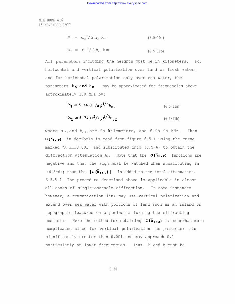
MIL-HDBK-41615 NOVEMBER 1977
a1 = dL1
2/2he1 km (6.5-10a)
a2 = dL 2
2/2he2 k m (6.5-10b)
All parameters including the heights must be in kilometers. For
horizontal and vertical polarization over land or fresh water,
and for horizontal polarization only over sea water, the
parameters may be approximated for frequencies above
approximately 100 MHz by:
(6.5-11a)
(6.5-11b)
where a1,2 and he1,2 are in kilometers, and f is in MHz. Then
in decibels is read from figure 6.5-4 using the curve
marked "K < 0.001" and substituted into (6.5-6) to obtain the
diffraction attenuation Ak. Note that the functions are
negative and that the sign must be watched when substituting in
(6.5-6); thus the is added to the total attenuation.
6.5.5.4 The procedure described above is applicable in almost
all cases of single-obstacle diffraction. In some instances,
however, a communication link may use vertical polarization and
extend over sea water with portions of land such as an island or
topographic features on a peninsula forming the diffracting
obstacle. Here the method for obtaining is somewhat more
complicated since for vertical polarization the parameter K is
significantly greater than 0.001 and may approach 0.1
particularly at lower frequencies. Thus, K and b must be
6-50
Downloaded from http://www.everyspec.com
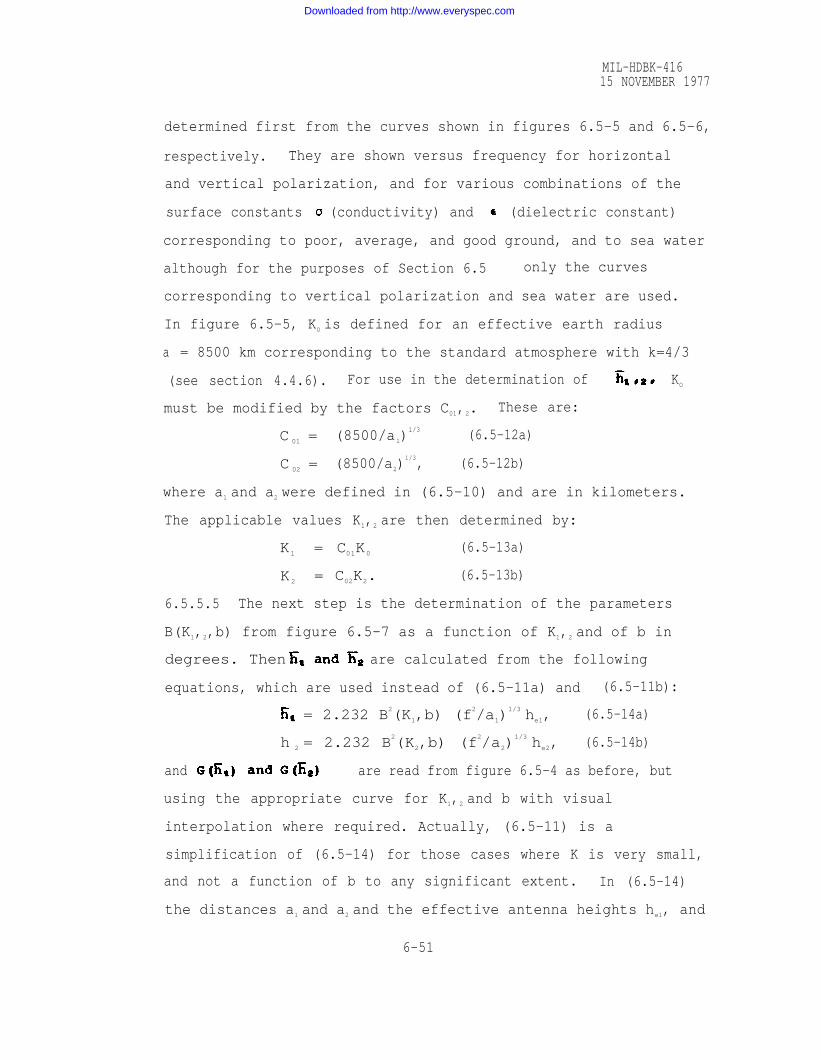
MIL-HDBK-41615 NOVEMBER 1977
determined first from the curves shown in figures 6.5-5 and 6.5-6,
respectively. They are shown versus frequency for horizontal
and vertical polarization, and for various combinations of the
surface constants (conductivity) and (dielectric constant)
corresponding to poor, average, and good ground, and to sea water
although for the purposes of Section 6.5 only the curves
corresponding to vertical polarization and sea water are used.
In figure 6.5-5, KO is defined for an effective earth radius
a = 8500 km corresponding to the standard atmosphere with k=4/3
(see section 4.4.6). For use in the determination of KO
must be modified by the factors C01,2. These are:
C 01 = (8500/a1)1/3 (6.5-12a)
C 02 = (8500/a2)1/3, (6.5-12b)
where a1 and a2 were defined in (6.5-10) and are in kilometers.
The applicable values K1,2 are then determined by:
K1 = C01K0(6.5-13a)
K 2 = C02K2. (6.5-13b)
6.5.5.5 The next step is the determination of the parameters
B(K1,2,b) from figure 6.5-7 as a function of K1,2 and of b in
degrees. Then are calculated from the following
equations, which are used instead of (6.5-11a) and (6.5-11b):
= 2.232 B2(K1,b) (f2/a1)
1/3 he1, (6.5-14a)
h 2 = 2.232 B2(K2,b) (f
2/a2)1/3 he2, (6.5-14b)
and are read from figure 6.5-4 as before, but
using the appropriate curve for K1,2 and b with visual
interpolation where required. Actually, (6.5-11) is a
simplification of (6.5-14) for those cases where K is very small,
and not a function of b to any significant extent. In (6.5-14)
the distances a1 and a2 and the effective antenna heights he1, and
6-51
Downloaded from http://www.everyspec.com

Figure 6.5-5
MIL-HDBK-41615 NOVEMBER 1977
6-52
Downloaded from http://www.everyspec.com

Figure 6.5-6
MIL-HDBK-41615 NOVEMBER 1977
6-53
Downloaded from http://www.everyspec.com

Figure 6.5-7
MIL-HDBK-41615 NOVEMBER 1977
6-54
Downloaded from http://www.everyspec.com

he2 must be in kilometers and the frequency f in
any parameter values outside the given range are
user should consult the original curves in [101]
MIL-HDBK-41615 NOVEMBER 1977
megahertz. If
encountered, the
or [102]. The
values in decibels are then substituted in (6.5-6) as
before to determine the attenuation Ak over the diffracting
obstacle.
6.5.5.6 In cases where terrain details over the entire path are
well known, and it is possible to identify pronounced reflecting
surfaces, four-ray geometric optics methods may be applicable
which must be modified to allow for attenuation and phase shift
of each ray by the diffracting obstacle. Applicable methods and
procedures for such cases are given in an appendix to MIL-HDBK-
417.
6.5.6 Attenuation Over A Rounded Knife Edge (See corresponding
paragraphs of section on "Attenuation over single-horizon
diffraction links" in MIL-HDBK-417.)
6.5.6.1 If the diffracting obstacle cannot be approximated by an
ideal knife edge; i.e., if its width at the top is more than
about 30 m, attenuation calculations must take into account the
rounding characterized by the parameter in (6.5-6). The
attenuation relative to free space can be estimated using the
dashed curve on figure 6.5-8 which represents an empirical
expression for mountain obstacle diffraction links, derived from
available data by Nishikori, et al. [103]. It may be used to
estimate without having to determine the curvature or
rounding of the diffracting knife edge. Note that the
curve in figure 6.5-8 departs from the solid curve for the ideal
knife edge indicated by A(v,0) only for values of v greater than
6-55
Downloaded from http://www.everyspec.com

MIL-HDBK-41615 NOVEMBER 1977
Figure 6.5-8 Empirical Obstacle Diffraction Loss.
6-56
Downloaded from http://www.everyspec.com

MIL-HDBK-41615 NOVEMBER 1977
approximately 7. The solid curve is the same as shown in figure
6.5-3 for v > 1 and given by (6.5-8) for v > 3. It is repeated
here for convenience and to illustrate the effects of rounding.
Note also that these effects have only been defined for v > 0;
i.e., where the obstacle protrudes into the path.
6.5.6.2 In some cases it is possible to estimate the rounding of
an isolated diffracting obstacle from detailed terrain profile
drawings or from map studies. The attenuation may then be
calculated more precisely. First, the radius of curvature r of
the obstacle is approximated by:
(6.5-15)
where Ds is the distance between radio horizon (from detailed
terrain profiles) in kilometers, and is in radians. Next, a
test is made to determine whether the obstacle is isolated from
the surrounding terrain using the relation:
kh[2/(kr)] 1/3 >> 1. (6.5-16)
Here, r is the radius of curvature of the rounded
obstacle from (6.5-15), and h is the smaller of the two values
and
with all distances and the wavelength in km. If the relation
in (6.5-16) does not hold for a specific path, the methods in
MIL-HDBK-417 (section on diffraction over irregular terrain)
should be used. Note that the term "isolated" is used here in a
different manner than in the determination of Fresnel zone
6-57
Downloaded from http://www.everyspec.com

MIL-HDBK-41615 NOVEMBER 1977
clearance for applicability of the height gain functions shown in
paragraph 6.5.5.2.
6.5.6.3 If the relation (6.5-16) holds, the rounding parameter,
is found by calculating the product using (6.5-17) below
and dividing by v which has been determined earlier (see
equation 6.5-7). The product will also be required in a
subsequent step.
(6.5-17)
Here the radio frequency f is in MHz, the radius of curvature r
from (6.5-15) is in km, and the angular distance is in radians.
6.5.6.4 The diffraction loss in decibels is plotted as a
function of v for various values of in figure 6.5-9. It may
also be determined from:
(6.5-18)
where the function A(v,0) is the attenuation for an ideal knife-
edge plotted in figures 6.5-3, 6.5-8 and 6.5-9, and the
functions are plotted in figure 6.5-10.
Equation (6.5-18) is applicable under many conditions of
propagation over irregular terrain between good antenna sites
using either horizontal or vertical propagation. Criteria for
its validity are (a) the distances d, d1, d2, and r must be much
larger than the wavelength, (b) the obstacle dimension at
right angles to the propagation path must be at least the width
of the first Fresnel zone, (c) the components (see
equation 6.5-5) of the diffraction angle must each be less than
0.175 radians, and (d) the radius of curvature, r, must be large
enough so that
6-58
Downloaded from http://www.everyspec.com

Figure 6.5-9
MIL-HDBK-41615 NOVEMBER 1977
6-59
Downloaded from http://www.everyspec.com

MIL-HDBK-41615 NOVEMBER 1977
Figure 6.5-10 The Functions A (O.P) and U(vp) in Odstacle Diffraction.
6-60
Downloaded from http://www.everyspec.com

MIL-HDBK-41615 NOVEMBER 1977
6.5.6.5 In summary, the single-obstacle diffraction
attenuation Ak may be obtained by calculating first the parameter
v, and using figure 6.5-8 or by calculating the parameter p in
addition to v and using (6.5-18): furthermore, the residual
height gain functions G(h1,2) calculated as shown in section
6.5.5 must be included where required. Values of basic
transmission loss are obtained by adding Ak and the median
atmospheric attenuation Aa, to the free-space loss, Lbf.
6.5.7 Fading and Long-term Variability
6.5.7.1 Fading on relatively short knife-edge diffraction links
(less than about 50 km) at frequencies above 5 GHz may be assumed
to be very similar in character to that discussed for line-of-
sight links in sections 4.2 and 4.4 of this handbook. It is quite
likely that multipath fading effects will predominate
particularly when reflections from the terrain on one or both
sides of the diffracting obstacle occur. Power fading due to
precipitation effects can also be treated as shown in sections
4.2.23 and 4.2.24. Diffraction fading as a result of
subrefractive conditions can be evaluated as shown in paragraph
6.5.7.3 below.
6.5.7.2 Long-term variability in the sense discussed in MIL-HDBK-
417 is usually not of primary importance for links that are less
than 50 km in length and operate at frequencies above about 5
GHz. The
amount to
long-term
estimates
variability of hourly medians in such cases should not
more than the 3 dB corresponding to the "degraded"
median value used as a basis for system performance
in the line-of-sight case (see section 4.5.18). For
longer paths, and for those at lower frequencies,
6-61
the methods
Downloaded from http://www.everyspec.com

MIL-HDBK-41615 NOVEMBER 1977
given in the sections on long-term variability and on service
probability in MIL-HDBK-417 should be used.
6.5.7.3 As already noted in paragraph 6.5.2.4, the expected
transmission loss variability over a knife-edge diffraction link
can also be associated with the variability of the effective
earth radius a as a function of changes in the average
refractivity gradient over the path. This is particularly
applicable when evaluating the effects of subrefractive
conditions where, with increasingly positive refractivity
gradients, a diffracting, obstacle intrudes more and more into the
free-space propagation path. Applicable cumulative time
distributions of initial refractivity gradients above the earth's
surface are given in [39] and [100] in terms of AN//lb as well as
of the effective earth radius factor k. Samples of such
distributions from [100] are shown in figure 6.5-11 together with
pertinent climate data. Note that these curves must be
extrapolated for extreme percentage values although there rarely
are sufficiently complete data to provide a good basis for
extrapolation.
6.5.7.4 In order to apply gradient distributions such as shown
in figure 6.5-11 to a design problem, diffraction transmission
loss calculations are performed using an appropriate range of
effective earth radius factor values, and then associating each
transmission loss value with the percentage of time corresponding
to the effective earth radius factor used. This method should be
used with caution since the data in the references cited above
represent observations at discrete locations and for very short
times only (i.e., once or twice daily). They are not necessarily
6-62
Downloaded from http://www.everyspec.com

MIL-HDBK-41615 NOVEMBER 1977
Gibraltar (British Colony)
36-09 N, 05-21 W. 3 meters MSLData: Radiosonde. 0000 and 12002 (0000 and 1200 LST)
1/68 - 12/70
Note : Calculated refractivity gradient between surface and nexthigher level. See text.
Analyzed by: Davis and Wagner, Environmental Technical ApplicationsCenter, U.S. Air Force, Washington, D.C.
Temperature (°F): January 60/50; July 83/68Mean Dewpoint (°F): January 48; July 63Precipitation (inches): Annual 32.1; January 6.06; July 0.04
Located on a 2.25 sq. mile peninsula on the southern tip of Spain. Mari-time climate with hot and nearly rainless summers and warm, rainy winters.
Figure 6.5-11 Examples of Refractivity Gradient Distributions.
6-63
Downloaded from http://www.everyspec.com

MIL-HDBK-41615 NOVEMBER 1977
representative of conditions occuring over a path of given
length, and all hours of the day. Boithias and Battesti [104]
give applicable estimates of the minimum effective value of the
effective earth radius factor k as a function of path length in a
continental temperate climate.
6.5.8 Worksheets for Diffraction Calculations And An Example.
6.5.8.1 Worksheets 6.5-1, 6.5-2, and 6.5-3 (on two pages) with
step-by-step procedures for knife-edge diffraction calculations
are included in this section. The various steps in the
calculations are referred to appropriate formulas, graphs, and
paragraphs in the text of section 6.5, or to earlier sections
or paragraphs in this handbook where appropriate.
6.5.8.2 As an illustrative example, filled-in worksheets are
also provided for an assumed 55 km link operating on 6 GHz using
vertical polarization. Figure 6.5-12 shows the assumed path
profile with the direct-ray path indicated for an effective earth
radius a = 8820 km corresponding to an average value of surface
refractivity Ns = 320 N-units. The path is assumed to go from
terminal 1 on an island off-shore via an on-shore obstacle to
terminal 2 on a hilltop farther inland so that one portion of the
path is over sea water. Inspection of the path profile also
suggests that sufficient clearance between the ray path and the
terrain is available for the overland portion of the path, but
not for the sea portion. Thus, the G(h1) function must be
calculated while the G(h2) function can be neglected. This is
also confirmed by use of the criteria given in paragraph 6.5.5.2.
It is also assumed that the obstacle is about 50 m (0.05 km) wide
6-64
Downloaded from http://www.everyspec.com

MIL-HDBK-41615 NOVEMBER 1977
at the top. In an actual case, this could be determined from
detailed maps or from a path survey.
6-65
Downloaded from http://www.everyspec.com

MIL-HDBK-41615 NOVEMBER 1977
Figure 6.5-12 Flat-Earth Profile for Knife-Edge Diffraction Example Path.
6-66
Downloaded from http://www.everyspec.com

fig. 6.5-1
6-67
Worksheet 6.5-1. Atmospheric and Terrain Perameters for Knife-edge Diffraction Calculations
Downloaded from http://www.everyspec.com
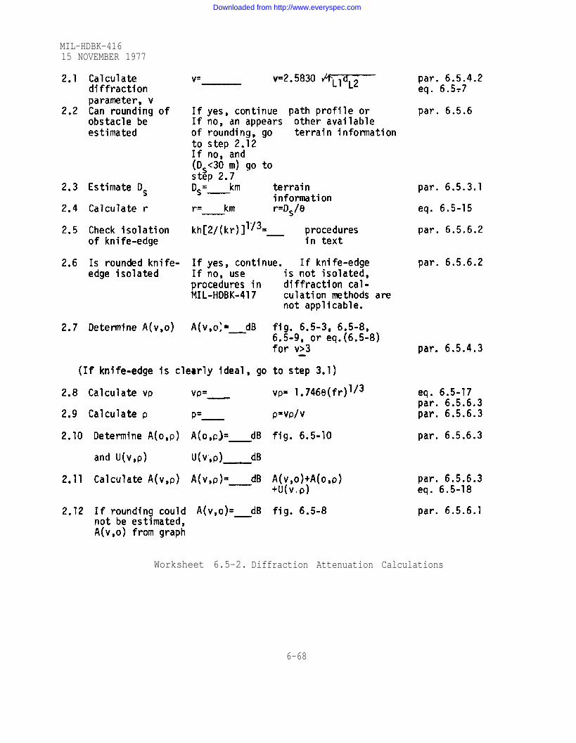
MIL-HDBK-41615 NOVEMBER 1977
Worksheet 6.5-2. Diffraction Attenuation Calculations
6-68
Downloaded from http://www.everyspec.com

MIL-HDBK-41615 NOVEMBER 1977
Worksheet 6.5-3. Effects of Ground Reflections and Diffraction Loss
6-69
Downloaded from http://www.everyspec.com

NOTE: The calculations in these worksheets may be performed for various valuesof the effective earth radius a in order to obtain a time distributionof Lbas discussed in paragraph 6.5.7.3.
Worksheet 6.5-3 (continued)
6-70
MIL-HDBK-41615 NOVEMBER 1977
Downloaded from http://www.everyspec.com

MIL-HDBK-41615 NOVEMBER 1977
Worksheet 6.5-1. Atmospheric and Terrain Parameters for Knife-edge Diffraction Calculations
6-71
Downloaded from http://www.everyspec.com

MIL-HDBK-41615 NOVEMBER 1977
Worksheet 6.5-2. Diffraction Attenuation Calculations
6-72
Downloaded from http://www.everyspec.com

MIL-HDBK-41615 NOVEMBER 1977
Worksheet 6.5-3. Effects of Ground Reflections and Diffraction Loss6-73
Downloaded from http://www.everyspec.com

MIL-HDBK-41615 NOVEMBER 1977
NOTE: The calculations in these worksheets may be performed for various valuesof the effective earth radius a in order to obtain a time distributionof Lb as discussed in paragraph 6.5.7.3.
Worksheet 6.5-3 (continued)
6-74
Downloaded from http://www.everyspec.com

15 NOVEMBER 1977
Section 6.6 ADDITIONAL BLANK WORKSHEETS
6.6.1 This section includes an additional set of blank worksheets forconvenience. They correspond to those in the text as follows:
Worksheet Page Number for
4.1-1
4.3-1
4.3-2
4.4-1
4.4.2
4.4-3
4.4-4
4.4-5
4.5-la
4.5-lb
4.5-2
4.5-3
4.5-4
4.5-5
4.5-6
4.5-7
4.5-8
4.5-9
4.5-10
4.5-11
6.5-1
6.5-2
6.5-3
Blank
4-5
4-80 and 4-81
4-120
4-121
4-234
4-235
4-236
4-266
4-267
4-268
4-269
4-270 and 4-271
4-272
4-273
4-274
6-67
6-68
6-69 and 6-70
6-75
Partially or CompletelyFilled-in (for Example)
4-85
4-117
4-118
4-119
4-312
4-313
4-260
4-314
4-315
4-316
4-317
4-318 and 4-319
4-320
4-321
6-71
6-72
6-73 and 6-74
MIL-HDBK-416
Downloaded from http://www.everyspec.com

MIL-HDBK-41615 NOVEMBER 1977
Current and future channel requirements for traffic
from site to site
Type ofChannel
Voice(Telephone)Voice(Facsimile)Voice(LOW Speed Data)Voice(Medium Speed Data)Digital Data(High Speed)
Video
Numberof
Channels
Basebandper
Channel Quality
Equivalent
voice chan-nels per infor-mation channel
Number ofequivalent
Totals
Link channel requirements
rounded to the next higher
nominal valuel
Transmitter RF bandwidth2
(Future Expansion)Voice(Telephone)Voice(Facsimile)Voice(low Speed Data)Voice(Medium Speed Data)Digital Data{High Speed)
Video
1 Nominal values are 24, 60, 120, 300, 600, 960, and 1800.
2 Estimate
Worksheet
using figure 4.1-1.
4. 1-1 Format for Recording Channel Requirements for FDM-FM Systems.
6-76
v o i c echannels
BasebandSpectrum
Downloaded from http://www.everyspec.com

MIL-HDBK-41615 NOVEMBER 1977
Site Name and Number
Latitude Longitude (Degrees, Min, See)
Map reference (most detailed topographic)
Nearest town (postoffice)
Access route: (all Year?)
Property owner; local contact:
Site sketch Site photograph General description
Reference baseline By Polaris Other
Antenna No. True bearing
Ground elev. MSL Takeoff angle (beam centerline
Takeoff angles to 45° right and left of centerline(Significant changes in horizon)
Critical Points: (include horizon)
Distance Map elev. Survey elev.
Tree height Required clearance
Description:
Horizon sketch Horizon photograph
Power availability:
a. Nearest transmission line b. Voltage
c. Frequency d. Phase e. Operating utility
Drinking water source Estimated depth to groundwater
Sewage disposal Type and depth of soil on and near site
Nearest airport railroad highway
navigable river
Worksheet 4. 3-1 Checklist for Site Survey (page 1 of 2)
6-77
Downloaded from http://www.everyspec.com

MIL-HDBK-41615 NOVEMBER 1977
Local communications facilities: telephone telegraph radio
Nearby radio transmitters relay stations
Other interference sources
Local transportation facilities: airlines railroads
truck bus
Warehouse and storage facilities
Local suppliers (hardware, lumbers concrete, etc.)
Local contractors
Fuel sources (oil, gas, propane)
Local housing accommodations: temporary permanent
Local military or civil contact
Meteorological data from local sources: (averages for each month)
Maximum/ minimum temperature (daily)
Precipitation (Also extreme 1- and 24-hour)
Snow depth (Also maximum for period of record)
Prevailing wind direction and speed— .
Extreme wind gust and direction
Dewpoint or relative humidity (mean diurnal change)
Worksheet 4. 3-1 Checklist for Site Survey (page 2 of 2)
6-78
.
Downloaded from http://www.everyspec.com

MIL-HDBK-41615 NOVEMBER 1977
DATE: OBSERVER:
SITE NAME and NUMBER:
LOCATION: Section Town Range
County State Country
REFERENCE MAPS:
DESCRIPTION:
ACCESS ROUTE:
SITE LOCATION SKETCH (not necessarily to scale)
Worksheet 4.3-2 Site Information Worksheet Blank6-79
Downloaded from http://www.everyspec.com

MIL-HDBK-41615 NOVEMBER 1977
Worksheet 4.4-1 Link Design Profile
6-80
Downloaded from http://www.everyspec.com

MIL-HDBK-41615 NOVEMBER 1977
Calculate h, the displacement of the curved earth radio path from the
flat earth path (section 4.2. 15).
d dh =1 2 where h is in m and dl and d2 in km. Calculate the dis-
12.75k
tance from the center line of the radio beam which will provide O. 6 of
first Fresnel zone clearance, 0.6 Rl (section 4.2.17).
For k = and f = GHz,
d1
d2 h 0.6R1
(km) (km) d 1d 2 (m) (m)
Worksheet 4.4-2 Link Design Clearance Calculations
6-81
Downloaded from http://www.everyspec.com

MIL-HDBK-41615 NOVEMBER 1977
A. Distance on Profile km.
Ground Elevation m above m.s.l.
Tree or Obstacle Height m above ground.
Total Obstruction Height m above m.s.l.
For an assumed upper antenna height of m, clearance of
m is realized for “k” = This provides(worst case)”
of Fresnel Zone clearance for this “k” value.(fraction) (order)
B. Distance on Profile km.
Ground Elevation m above m.s.l.
Tree or Obstacle Height m above ground.
Total Obstruction Height m above m.s.l.
For an assumed upper antenna height of m, clearance of
m is realized for “k” = This provides(worst case)”
of Fresnel Zone clearance for this “k” value.(fraction) (order)
C. Distance on Profile km.
Ground Elevation 1m above m.s..
Tree or Obstacle Height m above ground.
Total Obstruction Height 1m above m.s..
For an assumed upper antenna height of m, clearance of
m is realized for “k” = This provides
(worst case)”
of Fresnel Zone clearance for this “k” value.(fraction) (order)
Worksheet 4.4-3 Link Design Clearance Check
6-82
Downloaded from http://www.everyspec.com

MIL-HDBK-41615 NOVEMBER 1977
Worksheet 4.4-4. Link Design Summary, Part 1
6-83
Downloaded from http://www.everyspec.com

MIL-HDBK-41615 NOVEMBER 1977
Worksheet 4.4-5. Link Design Summary, Part 2
6-84
Downloaded from http://www.everyspec.com

Worksheet 4.5-1a 6-85
MIL-HDBK-41615 NOVEMBER 1977
Downloaded from http://www.everyspec.com

MIL-HDBK-416IS NOVEMBER 1977
6-86
Downloaded from http://www.everyspec.com

Worksheet 4.5-2 6-87
MIL-HDBK-41615 NOVEMBER 1977
Downloaded from http://www.everyspec.com
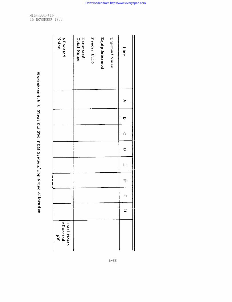
Worksheet 4.5-3
MIL-HDBK-41615 NOVEMBER 1977
6-88
Downloaded from http://www.everyspec.com

MIL-HDBK-41615 NOVEMBER 1977
Worksheet 4.5-4. Basic Parameters for Median Noise Calculations
6-89
Downloaded from http://www.everyspec.com

Worksheet 4.5-5. Transmitter Feeder Echo Noise Calculation
6-90
MIL-HDBK-41615 NOVEMBER 1977
Downloaded from http://www.everyspec.com
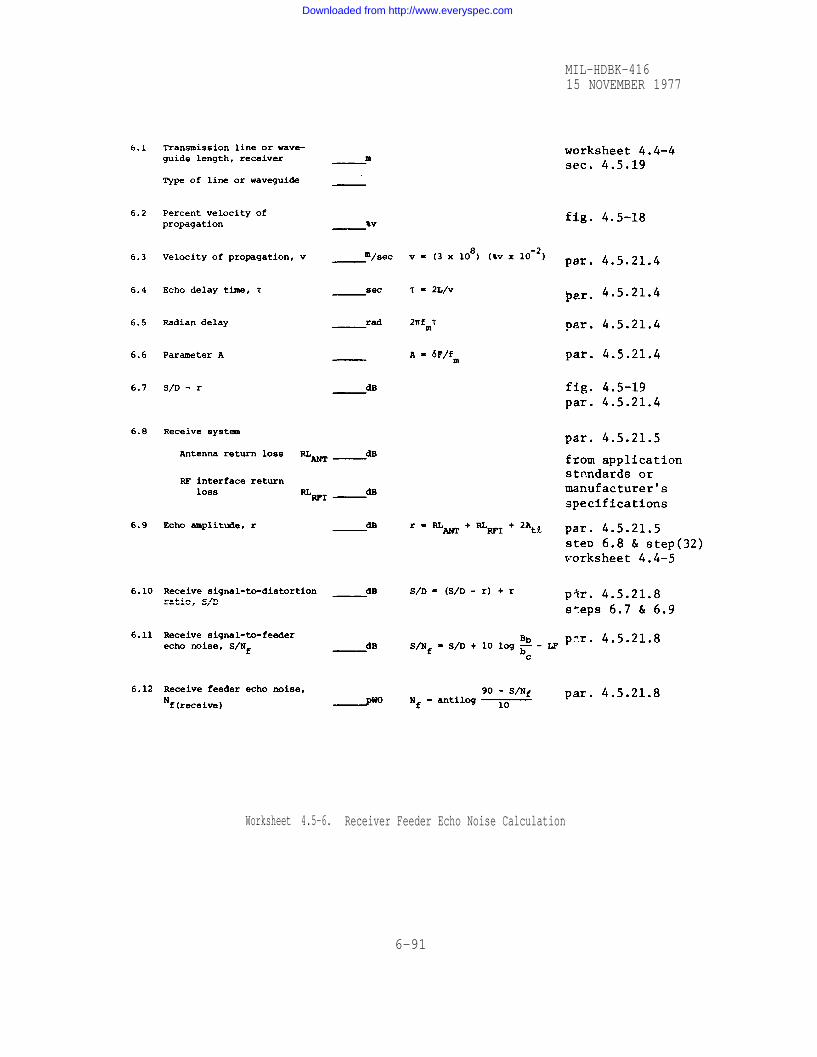
MIL-HDBK-41615 NOVEMBER 1977
Worksheet 4.5-6. Receiver Feeder Echo Noise Calculation
6-91
Downloaded from http://www.everyspec.com

MIL-HDBK-41615 NOVEMBER 1977
Note: Median values are denoted by (0.5).
Worksheet 4.5-7. Calculate Median Total Noise Performance
6-92
Downloaded from http://www.everyspec.com
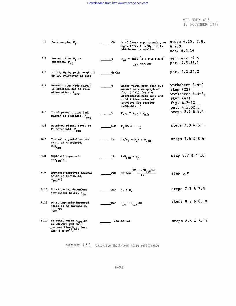
MIL-HDBK-41615 NOVEMBER 1977
Worksheet 4.5-8. Calculate Short-Term Noise Performance
6-93
Downloaded from http://www.everyspec.com
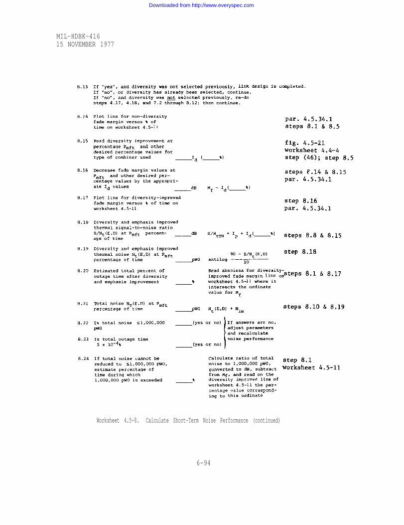
MIL-HDBK-41615 NOVEMBER 1977
Worksheet 4.5-8. Calculate Short-Term Noise Performance (continued)
6-94
Downloaded from http://www.everyspec.com
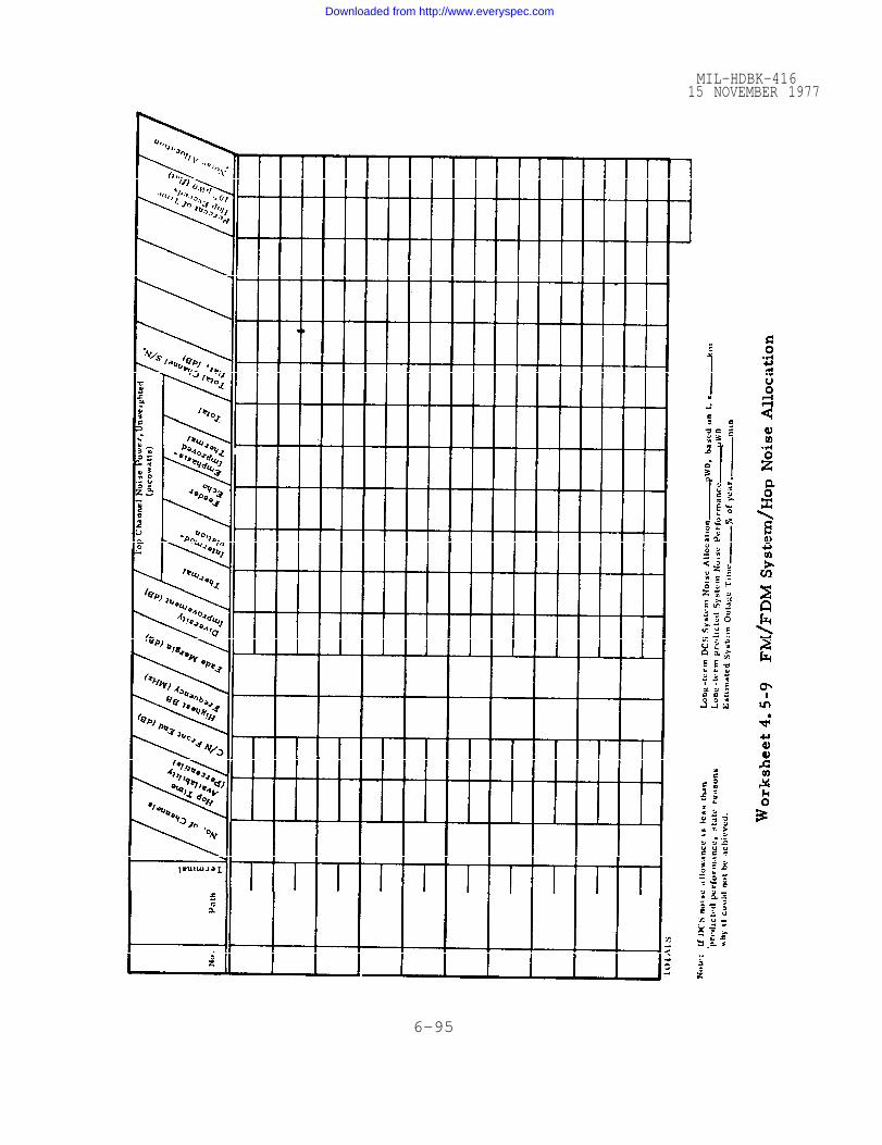
Worksheet 4.5-9
MIL-HDBK-41615 NOVEMBER 1977
6-95
Downloaded from http://www.everyspec.com

Worksheet 4.5-10. 6-96
MIL-HDBK-41615 NOVEMBER 1977
Downloaded from http://www.everyspec.com

Worksheet 4.5-11.
MIL-HDBK-41615 NOVEMBER 1977
6-97
Downloaded from http://www.everyspec.com

MIL-HDBK-41615 NOVEMBER 1977
Worksheet 6.5-1. Atmospheric and Terrain Parameters for Knife-edge Diffraction Calculations
6-98
Downloaded from http://www.everyspec.com

MIL-HDBK-41615 NOVEMBER 1977
6.5-2. Diffraction Attenuation CalculationsWorksheet
Downloaded from http://www.everyspec.com

MIL-HDBK-41615 NOVEMBER 1977
Worksheet 6.5-3. Effects of Ground Reflectiom and Diffraction Loss
6-100
Downloaded from http://www.everyspec.com
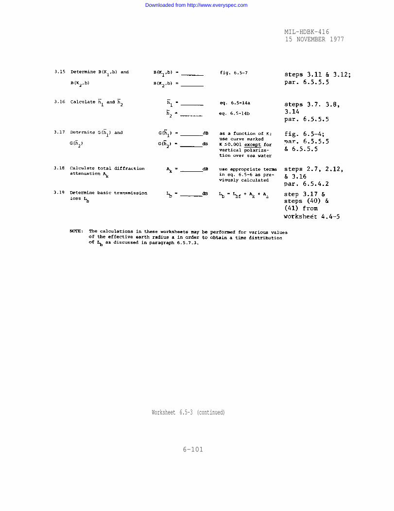
MIL-HDBK-41615 NOVEMBER 1977
Worksheet 6.5-3 (continued)
6-101
Downloaded from http://www.everyspec.com

THIS PAGE BLANK
6-102
Downloaded from http://www.everyspec.com

MIL-HDBK-41615 NOVEMBER 1977
CHAPTER 7
INDEX OF KEY TERMS
TERM
ABSORPTIONAtmospheric
ACTIVE REPEATERS
ADJACENT CHANNEL INFERENCE
AERIAL PHOTOGRAPHY
AERIAL RADAR SURVEYS
AIR CONDITIONING
ALARMS, FAULT
ALTIMETERS
ALTIMETER SURVEYS
AMPLIFIERSMicrowavePreamplifiersTraveling WaveRF
ANTENNABandwidthBeamwidthCarriageDimensionsDirectivityGainVSWRMountPatternPeriscopePlacement
ATMOSPHERIC ABSORPTION
PARAGRAPH NO.
4.2.22
4.4.46
4.5.11
4.3.16
4.3.15
5.5
5.7
6.2
4.3.13,6.2
4.4.444.4.454.4.444.4.44,4.4.45
4.4.294.4.294.4.296.44.4.294.4.294.4.294.4.294.4.304.4.294.4.385.1.2.3,5.8
4.2.22
ATMOSPHERIC LAYER PENETRATION 4.2.11
7-1
Downloaded from http://www.everyspec.com

MIL-HDBK-41615 NOVEMBER 1977
PARAGRAPH NO.TERM
ATTENUATIONAtmosphericFree SpacePrecipitationRainTransmission LineWaveguide
4.2.224.2.214.2.23,4.2.24,4.5.324.2.23,4.2.24,4.5.324.4.404.4.40
6.1AZIMUTH FROM POLARIS
4.1.3BANDWIDTH
6.2BAROMETERS
3.1,4.1.3BASEBAND
4.2.21
4.5.3
BASIC TRANSMISSION LOSS
BLOCK DIAGRAMS
5.1.5,5.2BUILDINGS
5.2.2.4 to 5.2.2.6CABLE
6.4.10CALIBRATION
CLEARANCEPathTerrain
4.2.174.3.12
4.2.31,4.3.3.3,4.3.22.3CLIMATOLOGICAL DATA
4.4.41COAXIAL CABLES
4.5.9CO-CHANNEL INTERFERENCE
4.4.25COMBINERS
4.5.4COMPATIBILITY, FREQUENCY
4.1.7CONSTRUCTION LIMITATION
4.4.26.6COSMIC AND SOLAR NOISE
4.5.8COUPLINGS, UNWANTED
6.1.1.2CULMINATION
7-2
Downloaded from http://www.everyspec.com

MIL-HDBK-41615 NOVEMBER 1977
TERM
DECLINATION
DECOUPLING,ANTENNA
DIFFRACTION,FADING
DIFFRACTION PATH
DIFFRACTORS
DIRECTIVITY
DISCRIMINATORS
DIVERSITY
DIVERSITY IMPROVEMENT
DIVERSITY RECEPTION
DUCTS, ATMOSPHERIC
DUCTS AND LAYERS
EARTH BULGE
EARTH’S RADIUS
EARTH RADIUS FACTOR
ECONOMIC RESTRAINT
EFFECTIVE RADIATED POWER
EIP - ENGINEERING IMPLEMENTATION PLAN
ELECTROMAGNETIC COMPATIBILITY (EMC)ECAC (EMC Analysis Center)HazardsNoiseSurvey
EQUIPMENTCommunication SystemMicrowave Separating and Combining ElementsAntennasLayout
PARAGRAPH NO.
6.1.1.4
4.4.13
4.4.12
4.4.39
4.4.39
4.4.29.8
4.4.45.8
4.4.22,4.5.34
4.5.34.1
4.4.22,4.4.23,4.4.244.5.34
4.4.14,4.4.18
4.4.14,4.4.9
6.4.2
4.2.15,4.4.6.2
4.4.6.2
4.1.5
4.4.29.17
4.1.12
5.84.2.33,5.8.35.1.2.4,5.84.4.26,5.84.2.33,4.3.3.3k
4.4.28,4.5.34.4.284.4.254.4.295.1,5.2
7-3
Downloaded from http://www.everyspec.com

MIL-HDBK-41615 NOVEMBER 1977
PARAGRAPH NO.TERM
4.4.314.4.404.4.444.4.454.4.464.36.4
Passive RepeatersTransmission LinesTransmittersReceiversActive RepeatersField SurveyPath Loss Testing
4.5.17,4.5.19EQUIPMENT PARAMETERS
4.5.18.3FADE MARGIN
FADING, K-TYPE 4.4.17
4.4.8 to 4.4.18FADING, L.O.S.
4.4.8 to 4.4.18FADING MECHANISMS
FADING, MULTIPATH 4.4.9,4.4.10,4.4.14
4.4.11 to 404.14FADING, POWER
4.2.23,4.4.15,4.5.32FADING, PRECIPITATION
4.2.27,4.4.21FADING RANGE ESTIMATES
4.4.18FADING, SURFACE DUCT
4.1.14FEASIBILITY
4.5.16,4.5.21FEEDER ECHO
4.3.4FIELD SUPPLIES
4.3FIELD SURVEY
4.3.44.3.24.3.3
EquipmentPlanningObjectives
4.4.43FILTERS
4.4.32 to 4.4.36FLAT REFLECTORS
4.2.26.6,4.2.31.8FOG
7-4
Downloaded from http://www.everyspec.com

MIL-HDBK-41615 NOVEMBER 1977
PARAGRAPH NO.T E R M
F R E Q U E N C YSelectionCompatibilityAllocationAssignmentRegulations
4.3.7,4.5.5, 4.5.74.5.44.1.10,4.5.54.1.10,4.5.54.5.6
FREQUENCY, CHOICE OF 4.5.7
FREQUENCY DIVERSITY 4.4.23
4.1.3,4.1.10,4.3.7FREQUENCY REQUIREMENTS
FRESNEL ZONES 4.2.18
4.2.18FRESNEL ZONE RADIUS
FRONT-TO-BACK RATIO 4.4.29.16
FUNCTIONAL REQUIREMENTS 4.1.2
FUTURE SYSTEM EXPANSION 4.1.2.3
4.4.29.4GAIN, ANTENNA
GEOLOGICAL DATA 4.3.3.3
GRADIENTS, REFRACTIVE INDEX 4.2.25,4.4.6
GREAT CIRCLE 4.2.16
GROUNDINGElectrical/ElectronicLightning
5.1.5.13,5.2.2.85.4.3
4.5.14,4.5.16HOP
HORN ANTENNA 4.4.29.1
HOUR ANGLE 6.1.1.1
IF REPEATER 4.4.46
IMPEDANCE 4.4.29.11
INSTALLATION PLANS 5.1,5.2
7-5
Downloaded from http://www.everyspec.com

MIL-HDBK-41615 NOVEMBER 1977
PARAGRAPH NO.TERM
INTERFERENCE 4 .2.33,4.4.26,4.4.274.5.9,4.5.13
4.5.94.5.104.5.114.5.12
Types ofCo-channelAdjacent ChannelDirect Adjacent Channel
INTERMODULATION NOISE CALCULATION 4.5.20,4.5.21
IONIZATION HAZARD 5.1.2.4,5.8
4.4.29.3ISOTROPIC ANTENNA
KNIFE-EDGE DIFFRACTION 4.4.39
K-TYPE FADING 4.4.17
LAYOUT, EQUIPMENT 4.5.2,4.5.3
4.4LINK DESIGN
LOCAL MEAN TIME 6.1.3
4.2.29LONG LINE-OF-SIGHT PATHS
4.4.5LOS PROPAGATION
4.2.4, 4.3.2.1, 4.4.3MAPS
MAP SCALE 4.2.14
4.3.11.1MARKERS, PERMANENT
MEASUREMENTS, PATH LOSS 4.3.11.17, 4.3.20
4.4.8MECHANISMS, FADING
METEOROLOGICAL DATA 4.2.31, 4.3.3.3
MIXER 4.4.45.4
MODULATION 4.4.44.3
4.2.26,4.2.27,4.4.84.4.9, 4.4.10
MULTIPATH
7-6
Downloaded from http://www.everyspec.com

MIL-HDBK-41615 NOVEMBER 1977
TERM
NOISEAdditiveAtmosphericGalacticTime InvariantLong-term Median ThermalMan-madeSolarThermalEquipment Intermodulation
PARAGRAPH NO.
4.4.264.4.26.54.4.26.64.5.224.5.234.4.26.84.4.26.64.5.23,4.5.164.5.20,4.5.21
NOISE ALLOWANCE 4.5.16,4.5.29
NOISE FIGURE 4.4.45.12
NOISE PERFORMANCE ESTIMATES 4.5.14
NOISE PERFORMANCE, LONG-TERM MEDIAN TOTAL 4.5.28
NOISE REQUIREMENTS 4.5.15
NOISE SOURCES 4.4.26.3
OBSTRUCTION LOSS 4.4.12
OPTICAL SURVEYS 4.3.14,6.3
OSCILLATORS, MICROWAVE 4.4.44.5
PARABOLIC-REFLECTOR ANTENNAS 4.4.29.21
PASSIVE REPEATERS 4.2.9,4.4.31
PATH CALCULATIONS 4.2.20,4.5.18
PATH CLEARANCE 4.2.17
PATH DESCRIPTION 4.3.3.3
PATH LOSS DISTRIBUTION 4.5.18
PATH LOSS MEASUREMENTS 4.2.36,4.3.20,6.4
PATH LOSS PREDICTIONS 4.2.20
PATH PERFORMANCE 4.3.20
PATH PROFILE 4.2.13,4.2.15,4.4.3
7-7
Downloaded from http://www.everyspec.com

MIL-HDBK-41615 NOVEMBER 1977
TERM
PERISCOPE ANTENNAS
PARAGRAPH NO.
4.4.38
4.3.2.3
6.1
4.4.29.28
PERSONNEL,SURVEY
POLARIS
POLARIZATION
POWERDesign,SystemDistribution Drawing
5.35.2.2.7
POWER AVAILABILITY 4.3.3.3
4.4.114.4.124.4.134.4.144.4.15
POWER FADINGDue to DiffractionDue to Antenna “Decoupling”Due to Ducts and LayersDue to Precipitation
POWER GAIN 4.4.29.4
4.2.23,4.4.15,4.5.32PRECIPITATION FADING
4.5.26PRE-EMPHASIS
PRIME MERIDIANS 4.2.4
PROFILE GRAPH PAPER 4.2.15
PROFILES, TERRAIN 4.2.13,4.2.15,4.4.3
4.4.5PROPAGATION
QUALITY 4.1.3
RADIATION HAZARD 5.1.2.4,5.8
RADIATION PATTERN 4.4.32
RADIO FREQUENCY (RF) 4.1.9,4.3.7,4.5.7
RADIO REGULATIONS 4.5.6
RAIN ATTENUATION 4.2.23,4.2.24,4.4.15,4.5.32
RAINFALL RATE 4.2.23,4.2.24
7-8
Downloaded from http://www.everyspec.com

MIL-HDBK-41615 NOVEMBER 1977
TERM
RAYLEIGH FADING
REAL ESTATE
RECEIVER
RECIPROCITY
REFLECTING SURFACE
REFLECTIONS, TERRAIN
REFLECTORSParabolicPlane
REFRACTION, ATMOSPHERIC
REFRACTION, INDEX OF
REFRACTIVITY GRADIENTS
REGULATIONS, RADIO
RELAY LINKS, POTENTIAL
RELAY SITES
REPEATERSActiveBasebandHeterodynePassiveThrough
RESOURCE LIMITATIONS
RF AMPLIFIERS
ROADS, ACCESS
ROUTEConsiderationsSelection
PARAGRAPH NO.
4.4.20
4.1.6
4.4.45
4.4.29.20
4.3.17.2,4.3.22.4,4.3.20.2,4.4.9,4.4.32
4.2.19,4.2.26,4.3.20.2,4.4.9,4.4.10
4.2.9.14.4.29.224.4.32 to 4.4.36
4.2.25,4.4.6
4.4.6
4.4.6,4.4.7
4.5.6
4.2.7
4.2.5
4.4.464.4.464.4.464.2.94.4.46
4.1.4
4.4.44,4.4.46
5.1.3
4.2.304.2.6
7-9
Downloaded from http://www.everyspec.com

MIL-HDBK-41615 NOVEMBER 1977
TERM
ROUTE ALTERNATIVES
ROUTES, DIRECT
ROUTE DIVERSITY
ROUTES, POTENTIAL
ROUTES, PRELIMINARY
SECURITY, SITE
SEISMIC DATA
SELECTIVE INTERFERENCE
SIGNAL INPUT, SHORT-TERM
SITE DESCRIPTION
SITE PLAN
SITE SELECTION
SITE VISITS
SITE VISITS, PERMISSION FOR
SITES
SITINGAccess
Contour MapField Trips
SOUTHERN HEMISPHERE
SPACE DIVERSITY
SPECTRUM, FREQUENCY
STANDARD ATMOSPHERE
SURVEY EQUIPMENT
PARAGRAPH NO.
4.2.35
4.2.8
4.2.6.2
4.2.6
4.2.12
4.2.34
4.3.3.3
4.4.27
4.5.31
4.3.3.3,4.3.11
5.1.2
4.2.2,4.3.23
4.3.11
4.3.10
4.2.2,4.2.5,4.2.10,5.1
4.2.5,4.3.3.3,4.3.104.3.11
4.2.44.3.3.3,4.3.11
6.1.1.6
4.4.22,4.4.23,4.5.34
4.1.9
4.2.15.1
4.3.4
7-10
Downloaded from http://www.everyspec.com
MIL-HDBK-41615 NOVEMBER 1977
TERM PARAGRAPH NO.
SURVEYFieldPlanningEquipment
4.34.3.24.3.2.2,4.3.4
SYSTEM LAYOUT 4.5.2
TEMPERATURE INVERSION 4.4.6.7
TERRAIN CLEARANCES 4.3.12
TERRAIN PROFILES 4.2.13,4.2.15,4.4.3
TERRAIN REFLECTIONS 4.2.19,4.2.19.5,4.4.9,4.4.10
TESTING, PATH LOSS 6.4
THRESHOLD LEVEL (FM) 4.5.18.3
THERMAL RECEIVER NOISE 4.4.45,4.5.23 to 4.5.27
TIMEApparentLocal MeanMean SolarSiderealStandardZone BoundariesGreewich Civil
6.1.36.1.36.1.36.1.36.1.36.1.36.1.3
TIME AVAILABILITY 4.5.36 to 4.5.38
TIME REQUIREMENTS, SURVEY 4.3.8
TOWERS 4.1.7,4.2.32,4.3.17.3,4.4.4,5.4
TOWERS FOR PATH LOSS TESTING 4.3.17.3
TRANSMISSION LINES, RFLayoutTypes
4.4.405.2.2.105.6
TRANSMISSION LOSS 4.2.21
TRANSMITTERS 4.4.44
TRANSPORTATION 4.3.5
7-11
Downloaded from http://www.everyspec.com

MIL-HDBK-41615 NOVEMBER 1977
TERM PARAGRAPH NO.
TRAVELING WAVE TUBE AMPLIFIERS 4.4.44.7
4.2.14.2UTM GRID
VSWR = VOLTAGE STANDING WAVE RATIO 4.4.29.13,4.5.21.5
4.5.21.4, 4.5.21.5WAVE VELOCITY
3.1, 4.2.18WAVELENGTH
WAVEGUIDEDehydratorLayoutTypes
4.4.42, 4.5.195.6.3.25.2.2.105.6
ZONESFresnelRain RateTime
4.2.184.2.246.1
4.1.6, 4.1.7ZONING RESTRICTIONS
Custodians:Army - SCNavy - ECAir Force - 17
Preparing ActivityAir Force - 17
(Project SLHC-0023)Review Activities:Army - SC, ELNavy - AS, SHAir Force - 1,11,13,71
Other InterestJCS - J6
User Activities:Army -Navy -Air Force -
7-12
*U.S. GOVERNMENT PRINTING PFFICE:1988 505-033/91286
Downloaded from http://www.everyspec.com

Downloaded from http://www.everyspec.com
Downloaded from http://www.everyspec.com