
Miguel Lourenço Rodrigues Master’s thesis in Biomedical Engineering December 2011 1.
43
A Bayesion perfusion estimation using spatio-temporal priors in ASL-MRI Miguel Lourenço Rodrigues Master’s thesis in Biomedical Engineering December 2011 1
-
Upload
lorena-leeming -
Category
Documents
-
view
214 -
download
0
Transcript of Miguel Lourenço Rodrigues Master’s thesis in Biomedical Engineering December 2011 1.

1
A Bayesion perfusion estimation using spatio-temporal priors in
ASL-MRIMiguel Lourenço Rodrigues
Master’s thesis in Biomedical EngineeringDecember 2011

2
Outline
1. Introduction and Objectives
2. Methods: Problem Formulation, Simulations and Real Data
3. Results and Discussion
4. Conclusions

Outline
1. Introduction
2. Literature Review
3. Problem Formulation
4. Experimental Results and Discussion
5. Conclusions
3

4
Introduction
-Cerebral Blood Flow (CBF):
Volume of blood flowing per unit time[2]
-Perfusion:
CBF per unit volume of tissues
Arterial Spin Labeling (ASL):
-Non invasive technique for generating perfusion images of the brain [1]
Se [1] e [2] são refs, deviam aparecer antes com nome e ano
5
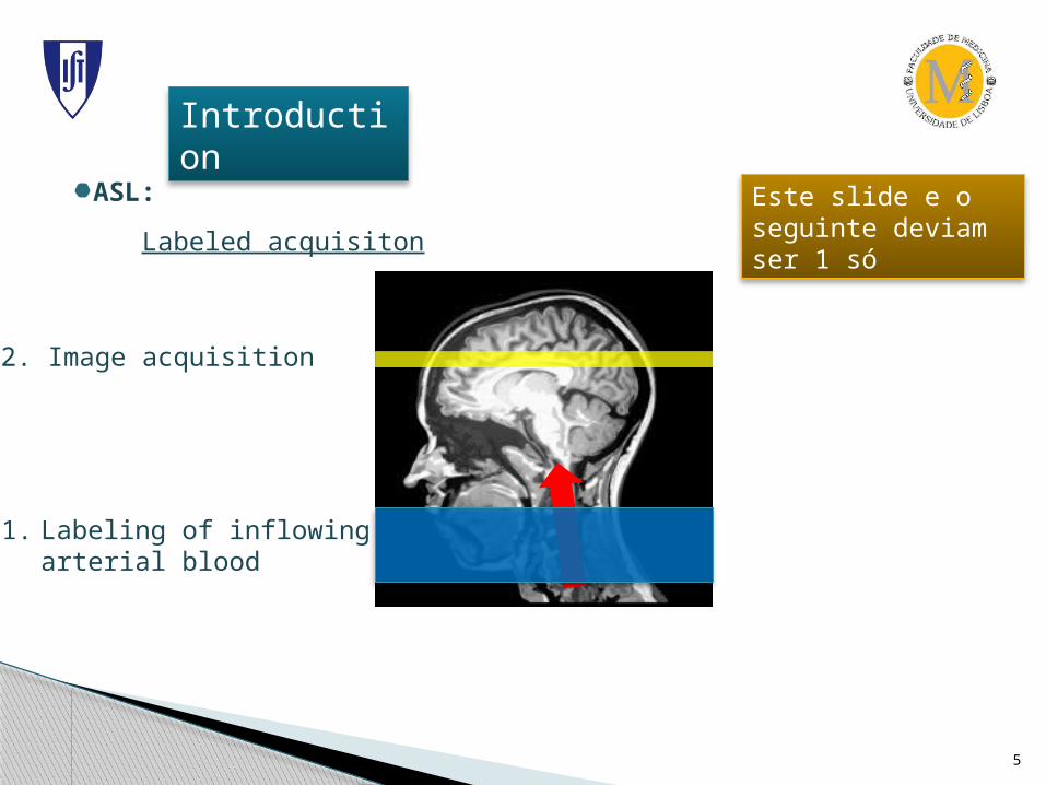
Introduction
Labeled acquisiton
1. Labeling of inflowingarterial blood
2. Image acquisition
ASL: Este slide e o seguinte deviam ser 1 só

6
Introduction
ASL
Control acquisiton
3. No labeling
4. Image acquisition
7
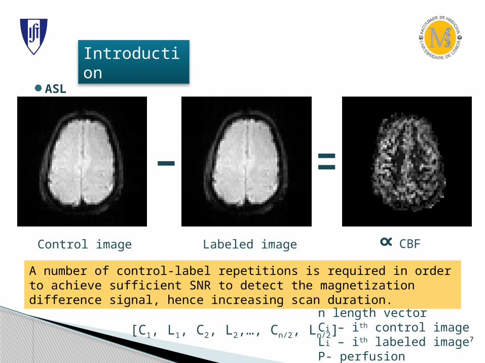
Introduction
ASL
Control image Labeled image CBF
A number of control-label repetitions is required in order to achieve sufficient SNR to detect the magnetization difference signal, hence increasing scan duration.
[C1, L1, C2, L2,…, Cn/2, Ln/2] n length vectorCi – ith control imageLi – ith labeled imageP- perfusion

8
Introduction
ASL signal processing methods
Pair-wise subtraction:
[P1, P2,…, Pn/2]=[C1- L1, C2- L2,…, Cn/2-Ln/2]
Surround subtraction:
[P1, P2,…, Pn/2]=[C1- L1, C2- (L1+L2),…, Cn/2-(L(n/2)-1-Ln/2)] 2 2
Sinc-interpolated subtraction:
[P1, P2,…, Pn/2]=[C1- L1/2, C2- L3/2,…, Cn/2-Ln/2-1/2]

9
Objectives
Objectives
-Increase image Signal to Noise Ratio (SNR)
-Reduce acquisition time
Approach
- New signal processing model
- Bayesian approach
- spatio-temporal priors
No drastic signal variatons
(except in organ boundaries)

10
Outline
1. Introduction
2. Literature Review
3. Problem Formulation
4. Experimental Results and Discussion
5. Conclusions

11
Problem Formulation
Mathematical model
Y(t)=F+D(t)+v(t)ΔM+Γ(t)
Y (NxMxL) – Sequence of L PASL images
F (NxM) – Static magnetization of the tissues
D(NxM x L) – Slow variant image (baseline fluctuations of the signal – Drift)
v(L x 1) - Binary signal indicating labeling sequences ΔM(NxM ) - Magnetization difference caused by the inversion
Γ(NxM xL) – Additive White Gaussian Noise ~N (0,σy2)
(1)

12
Problem Formulation
Mathematical model
Y(t)=F+D(t)+v(t)ΔM+Γ(t) (1)

13
Problem Formulation
Algorithm implementation
Y(t)=F+D(t)+v(t)ΔM+Γ(t) (1)
Vectorization
Y=fuT+D+ΔmvT+Γ
Y(NM x L)
f(NM x1)
u(L x 1)
D(NM x L)
v(L x 1)
Δm(NM x 1)
Γ(NM x 1)
(2)

14
Problem Formulation
Algorithm implementation
Since noise is AWGN,
p(Y)~N (μ, σy2), where μ=fuT+D+ΔmvT
Maximum likelihood (ML) estimation of unknown images, θ={f,D, Δm}
θ=arg min Ey(Y,v,θ)θ
Ill-posed problem
(3)

15
Problem Formulation
Algorithm implementation
Using the Maximum a posteriori (MAP) criterion, regularization isintroduced by the prior distribution of the parameters
θ=arg min Ey(Y,v,θ)θ
(3)
θ=arg min E (Y,v,θ)θ
(4)
E (Y,v,θ)=Ey (Y,v, θ) + Eθ(θ) (5)
Data – fidelity term Prior term

16
Problem Formulation
Algorithm implementation
Figure from [11]

17
Problem Formulation
Algorithm implementation
E (Y,v,θ)=Ey (Y,v, θ) + Eθ(θ) (5)
½ Trace [(Y-fuT-D-ΔmvT) T (Y-fuT-D-ΔmvT)] E (Y,v,θ)=
+αTrace[(φhD)T(φhD)+(φvD)T(φvD)+(φtD)T(φtD)]
+β(φhf)T(φhf)+(φvf)T(φvf)
+γ(φhΔm)T(φhΔm)+(φvΔm)T(φvΔm)
(6)

18
Problem Formulation
Algorithm implementation
-In equation (6), the matrices φh,v,t are used to compute the horizontal, Vertical and temporal first order differences, respectively
1 0 0 . -1
-1 1 0 . 0
0 -1 1 0
. . . . .
. . . . .
. . . . 0
0 0 . -1 1
Φ=
-α, β and γ are the priors.

19
Problem Formulation
Algorithm implementation
-MAP solution as a global mininum
-Stationary points of the Energy Function – equation (6)
- Equations implemented in Matlab and calculated iteratively
20
Outline
1. Introduction
2. Literature Review
3. Problem Formulation
4. Experimental Results and Discussion
5. Conclusions

21
Experimental Results and Discussion
Synthetic data
-Brain mask (64x64)
-Axial slice
-White matter (WM) and Gray matter (GM)
ISNR=SNRf-SNRi
∑100
NxM
N,M
i=1,j=1
|xi,j-xi,j|
xi,j
^
Mean error(%)=
SNR=Asignal
Anoise
2
- ;
-
22
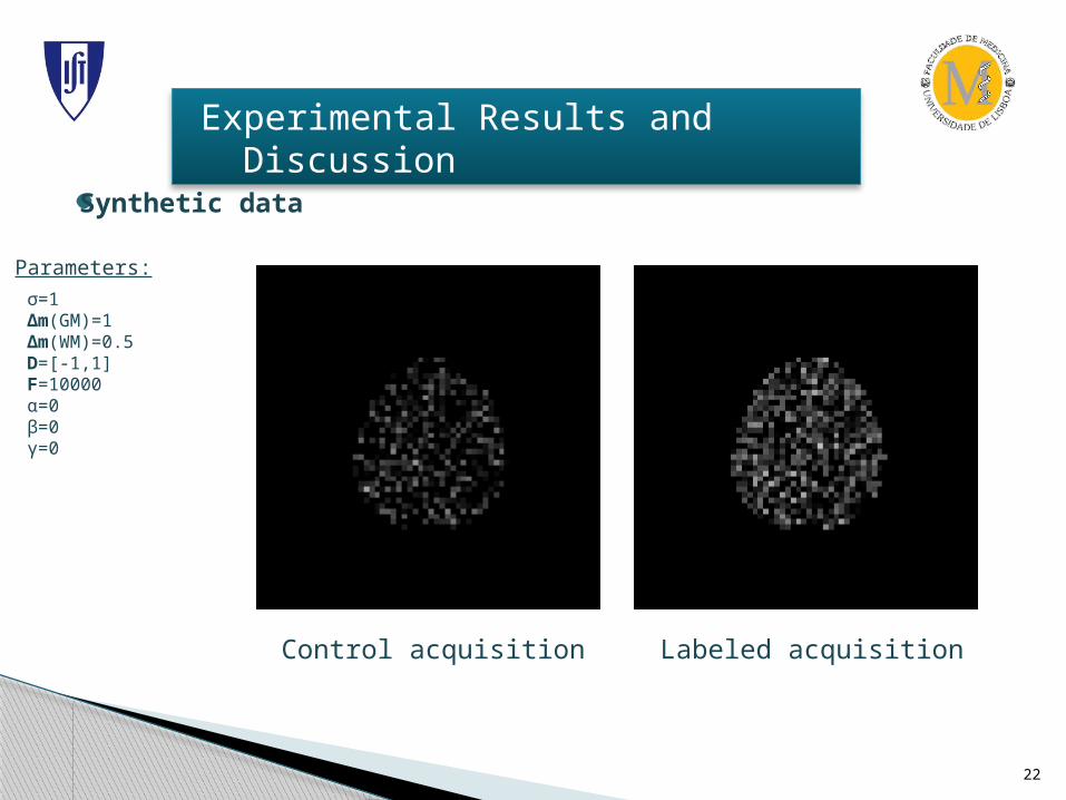
Experimental Results and Discussion
Synthetic data
Control acquisition Labeled acquisition
Parameters:
σ=1Δm(GM)=1Δm(WM)=0.5D=[-1,1]F=10000α=0β=0γ=0
23
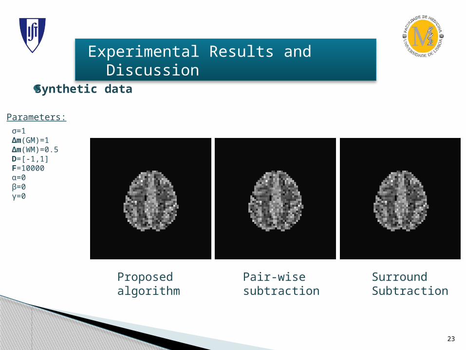
Experimental Results and Discussion
Synthetic data
Proposed algorithm
Pair-wisesubtraction
SurroundSubtraction
Parameters:
σ=1Δm(GM)=1Δm(WM)=0.5D=[-1,1]F=10000α=0β=0γ=0

24
Experimental Results and Discussion
Synthetic data
Method ISNR(dB)
Mean Error (%)
Proposed algorithm 13.906 24.658
Pair-wise subtraction 13.906 24.658
Surround Subtraction 13.999 24.393
25
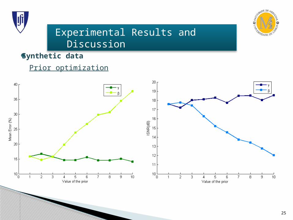
Experimental Results and Discussion
Synthetic data
Prior optimization

26
Experimental Results and Discussion
Synthetic data
Prior optimization
Incresasing prior value

27
Experimental Results and Discussion
Synthetic data
Prior optimization

28
Experimental Results and Discussion
Synthetic data
Prior optimization
β=1γ=5

29
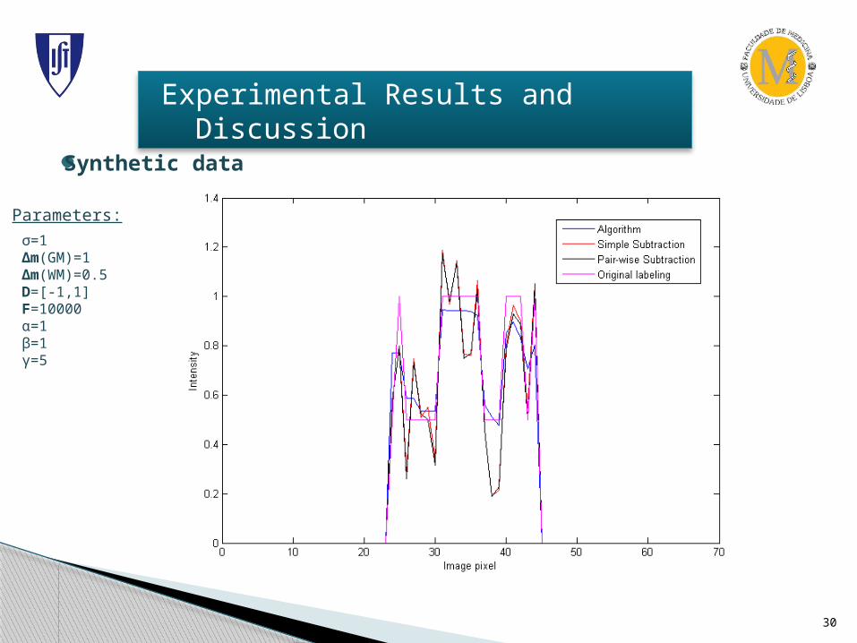
Experimental Results and Discussion
Synthetic data
Parameters:
σ=1Δm(GM)=1Δm(WM)=0.5D=[-1,1]F=10000α=1β=1γ=5
Proposed algorithm
Pair-wisesubtraction
SurroundSubtraction
30
Experimental Results and Discussion
Synthetic data
Parameters:
σ=1Δm(GM)=1Δm(WM)=0.5D=[-1,1]F=10000α=1β=1γ=5

31
Experimental Results and Discussion
Synthetic data
Method ISNR(dB)
Mean Error (%)
Proposed algorithm 16.990 17.807
Pair-wise subtraction 14.026 24.492
Surround Subtraction 14.103 24.269

32
Experimental Results and Discussion
Synthetic data
Method ISNR(dB)
Mean Error (%)
Proposed algorithm 16.990 17.807
Pair-wise subtraction 14.026 24.492
Surround Subtraction 14.103 24.269
3dB
7%
23%
-30%

33
Experimental Results and Discussion
Synthetic data
Monte Carlo Simulation for different noise levels

34
Experimental Results and Discussion
Real data
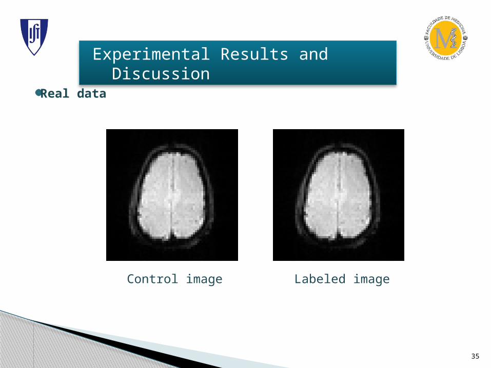
-One healthy subject
-3T Siemens MRI system (Hospital da Luz, Lisboa)
-PICORE-Q2TIPS PASL sequence
-TI1/TI1s/TI2=750ms/900ms/1700ms
-GE-EPI
-TR/TE=2500ms/19ms
-201 repetitions
-spatial resolution: 3.5x3.5x7.0 mm3
-Matrix size: 64x64x9
35
Control image Labeled image
Experimental Results and Discussion
Real data

36
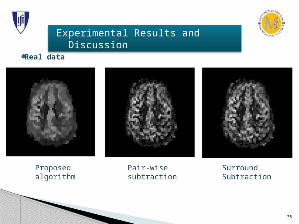
Experimental Results and Discussion
Real data
Proposed algorithm
Pair-wisesubtraction
SurroundSubtraction

37
Experimental Results and Discussion
Real data
-Influence of thenumber of iterations
38
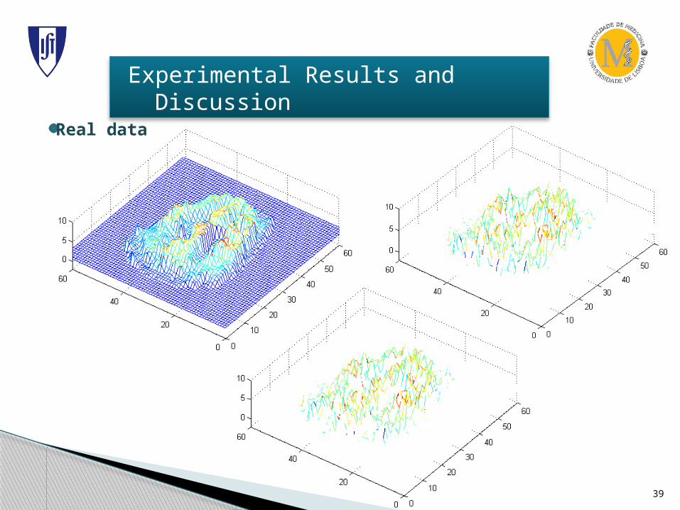
Proposed algorithm
Pair-wisesubtraction
SurroundSubtraction
Experimental Results and Discussion
Real data
39
Experimental Results and Discussion
Real data

40
Outline
1. Introduction
2. Literature Review
3. Problem Formulation
4. Experimental Results and Discussion
5. Conclusions

41
Conclusion
-The proposed bayesian algorithm showed improvement of SNR and ME
-SNR increased by 3db (23%)
-ME decreased by 7% (30%)
-Applied to real data
Future work:
-Automatic prior calculation
-Reducing the number of control acquisitions
-Validation tests on empirical data

42
[1] T.T. Liu and G.G. Brown. Measurement of cerebral perfusion with arterial spin labeling: Part 1. Methods. Journal of the International neuropsychological Society, 13(03):517-525, 2007.
[2]A.C. Guyton and J.E. Hall. Textbook of medical physiology. WB Saunders (Philadelphia),1995.
[4]ET Petersen, I. Zimine, Y.C.L. Ho, and X. Golay. Non-invasive measurement of perfusion: a critical review of arterial spin labeling techniques. British journal of radiology, 79(944):688, 2006.
[3]D.S. Williams, J.A. Detre, J.S. Leigh, and A.P. Koretsky. Magnetic resonance imaging of perfusion using spin inversion of arterial water. Proceedings of the National Academy of Sciences, 89(1):212, 1992.
[5]R.R. Edelman, D.G. Darby, and S. Warach. Qualitative mapping of cerebral blood flow and functional localization with echo-planar mr imaging and signal targeting with alternating radio frequency. Radiology, 192:513-520, 1994.
Bibliography
[6]DM Garcia, C. De Bazelaire, and D. Alsop. Pseudo-continuous ow driven adiabatic inversion for arterial spin labeling. In Proc Int Soc Magn Reson Med, volume 13, page 37, 2005.
[7]E.C. Wong, M. Cronin, W.C. Wu, B. Inglis, L.R. Frank, and T.T. Liu. Velocity-selective arterial spin labeling. Magnetic Resonance in Medicine, 55:1334{1341, 2006.
[8]W.C. Wu and E.C. Wong. Feasibility of velocity selective arterial spin labeling in functional mri. Journal of Cerebral Blood Flow & Metabolism, 27(4):831{838, 2006
[9]GK Aguirre, JA Detre, E. Zarahn, and DC Alsop. Experimental Design and the Relative Sensitivity of BOLD and Perfusion fMRI. NeuroImage, 15:488{500, 2002.
[10]E.C. Wong, R.B. Buxton, and L.R. Frank. Implementation of Quantitative Perfusion Imaging Techniques for Functional Brain Mapping using Pulsed Arterial Spin Labeling. NMR in Biomedicine, 10:237{249, 1997.
[11] J.M. Sanches, J.C. Nascimento, and J.S. Marques. Medical image noise reduction using the Sylvester-Lyapunov equation. IEEE transactions on image processing, 17(9), 2008.

43
Questions