MIGRATION OF CONTROL IN DECISION MAKING ORGANIZATIONS 1

JUNE 1989 LIDS-P-1881

MIGRATION OF CONTROLIN DECISION MAKING ORGANIZATIONS 1

Alexander H. Levis 2

Sabina L. Skulsky

Laboratory for Information and Decision Systems

Massachusetts Institute of Technology

Cambridge, MA 02139 USA

ABSTRACT

In a distributed decision making organization supported by information processing and decisionaiding systems, it is not always apparent whose decision affects the outcome the most. Often,control migrates away from the designated organization member in unexpected ways dependingon the decisions of individual decision makers, on the structure of the organization, and on itsoperating procedures. A mathematical formulation of the concept of migration of control and ofregions of dominance is given; the model and the computational procedure are illustrated by twosimple examples. The point is made that the introduction of technologies that allow distributeddecision making bring into focus dynamic phenomena that need novel approaches and newconcepts to describe them.

This work was supported in part by the Office of Naval Research under Contract No.N00014-84-K-0519.

2 Corresponding Author:Dr. Alexander H. Levis, MIT, 35-410/LIDS, Cambridge, MA 02139, USA

Levis and Skulsky: Migration of Control ... IDT - 890522

INTRODUCTION

M. Van Creveld in his book Command in War [13] makes the case that while the problem of

command or management of an organization is not new, "its dimensions have grown exponentially

in modem times, especially since 1939." Indeed, the increase in the demands made on the

information and decision systems supporting modem organizations can be attributed in part to the

wide geographical distribution of the resources or assets managed by the organization, the

complexity of the environment in which the organization functions, and the rate at which this

environment changes, the so-called tempo of operations [7]. Another part of the problem has been

caused by the technologies themselves, data processing and communications, that were introduced

as a means for coping with the distributed nature of the organizations.

The interaction of organizations that try to carry out distributed decision making with the

information and decision technologies introduced to aid them is either generating new classes of

phenomena not previously observable, or is bringing to the fore organizational problems that were

previously of secondary importance. Examples of the results of such interaction are the large

amounts of data collected and processed, the proliferation of displays for presenting information in

a form suitable for supporting decision making at different echelons of an organizational hierarchy

or different levels of a functional hierachy, or the massive exchange of data and information

among the nodes of a distributed organization.

The development of effective systems that process data and convert it to information and then

frame it to support decision making depends not only on the available technology - the sensors, the

computers, the communications systems, and the displays and human-computer interfaces - but

also on the structure of the decision making organizations themselves and the cognitive processes

embedded in the organization members, the concept of operations that governs their interactions,

and the intelligent machines that support them. The relationship between data and information, and

information and the knowledge needed to make a decision are shown in Figure 1.[9]

DATA1I <= Technological

INFORMATIONXI <= Cognitive

KNOWLEDGE

Figure 1. Data, Information, and Knowledge

2

Levis and Skulsky: Migration of Control ... IDT- 890522

Data are transformed to information primarily by technological processing: time series residing

in a data base are presented in the form of a graph on the monitor of a workstation. Humans can

also be part of the processing by executing comparable tasks. However, the transformation of

information into knowledge is a cognitive process done primarily by humans. The introduction of

intelligent decision support systems will shift these boundaries and will blur the demarkation lines

between technological and cognitive processing.

In this context, the human decision maker continues to occupy a central role in distributed

decision making organizations. The structure of the organization affects the human decision

maker's ability to work effectively under time pressure in a stressful environment ,such as the one

experienced by air traffic controllers, bond or foreign exchange traders, military commanders in

battle, or the operators of the control center of a power plant during an emergency. Furthermore,

the organization may exhibit dynamic phenomena not anticipated by analyzing the formal

organizational structure or the properties of the decision support system that is in place. One such

phenomenon is the migration of control.

Control refers to the result of processing the externally produced statements of system

requirements and analyzing system behavior in the presence of uncertainty. The migration of

control in an organization refers to the movement of the control function through the information

structure of a system. There is much anecdotal experience from large scale organizations that at

times control may migrate in an unpredictable manner away from decision makers who have been

assigned specific authority and responsibility to other organization members, usually at a lower

echelon. Changes in the organization's structure, such as access to decision support systems, can

change the sensitivity of the performance measures to the actions of different decision makers.

Furthermore, the choice of strategies on the part of these decision makers affects which one has

most impact on performance.

This migration of control can be viewed from both positive and negative perspectives. In the

former sense, it is desirable for control to migrate in the event of a failure of a decision making

node. Kahne [6] has highlighted this positive connotation while discussing control migration in a

command, control, and communication system. To maintain system performance, the control

function must be able to move (migrate) through a large scale system so that, if there are structural

changes in the system, deterioration of function will be minimized.

However, from a negative perspective, control may migrate in an unforeseen or undesirable

manner. For example, migration might occur away from executives, who should hold the positions

of responsibility in favor of subordinates. The performance of an organization will deteriorate if

what are seen to be efficient and effective means of processing information are altered upon

migration of control. Even if the structure is designed so that the overall task is performed without

3


overloading organization- members, that same structure can result in a wide range of performance

depending on the strategies chosen by the decision makers. It is important to insure that strategies

which are mutually acceptable will most likely be selected.

The main objective of this paper is to develop a model that shows the existence of migration of

control in organizations and to examine the circumstances under which it can occur. It is also

important from the analysis and design points of view to be able to determine how the migration

occurs and which decision maker becomes dominant. Thus, the first goal is to determine for some

candidate structures the sets of conditions for which a single decision maker becomes critical. The

second goal is to identify the causes for migration of control in the organization so that rules can

be developed for redesigning the protocols of the organization, or restructuring it, to avoid

undesired migrations. One method for doing so is restructuring the organization so as to avoid

undesirable control situations.

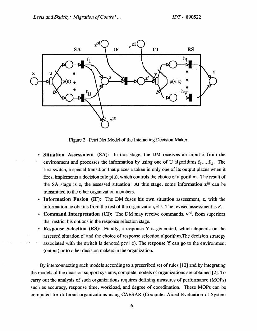
The technical approach that has been used in this paper consists of three steps. In the first

step, the model of the organization is developed and expressed in the form of a Petri Net. Included

in the specification of the problem is the set of tasks to be performed and the set of outputs that can

be produced by the organization. Furthermore, the space of behavioral strategies and a

performance index that assigns a value to each possible input-output pair are defined.The model of

the organization is used to relate inputs and outputs in terms of the particular behavioral strategy

chosen. In the second step, this relationship is made explicit by obtaining the mapping of the

strategy space into the performance space. Thus, for each point in the strategy space, a

corresponding value of the performance index is obtained. The key operation now is the

determination of a set of sensitivity coefficients: the sensitivity of the performance to changes in the

decisions of each decision maker. Thus, for each decision maker a value of his sensitivity

coefficient is obtained for each point of the performance space. By comparing the values of the

sensitivity coefficients of the different DMs at a point in the performance space, it is possible to

determine who is dominant at that point: he who has more of an impact on the value of the

performance, i.e., the one with the highest absolute value of the sensitivity coefficient. In this third

and last step, the information on who is the dominant DM at each point on the performance space is

mapped back to the strategy space to define the regions of dominance, if any, where certain

decision makers are in control. Then the designer can assess whether this migration of control from

one DM to another, as described by the regions of dominance, is desirable or not. He can then

trace throught the mappings and the models the reasons that dominance shifted from one to another

and, if necesary, make design modifications.

The results of this work are directed toward practical methods for increasing the efficiency of

information flow in large scale organizations.

4


PETRI NET MODELS AND ORGANIZATIONS

The mathematical framework that is used to model the structure of the organization and the

interactions between the decision makers is that of Petri Nets. A very brief introduction to.the.

formalism of Petri Nets follows.

A Petri Net - denoted by PN - is a bipartite directed graph represented by the quadruple

PN = (P, T, I, O), where P is a finite set of places, denoted by circle nodes, T is a finite set of

transitions, denoted by bar nodes, and where I and O are mappings that correspond to the set of

directed arcs from places to transitions (inputs) and from transitions to places (outputs). When I

and O take values in {0, 1}, where 0 denotes the absence of an arc and 1 the presence with

capacity 1, the resulting nets, called ordinary Petri Nets, are graphical tools used to model

concurrent and asynchronous processes. They represent the decision makers working in parallel

with one another and coordinating their activities. They can be used to model manufacturing

processes, represent flow charts of computer software, and in numerous other applications. They

are especially useful for modeling decision making organizations, since they show explicitly the

interactions among decision makers. An introduction to Petri Nets can be found in Reisig[1 1].

Petri Nets can be used to study the dynamics of decision making organizations by introducing

tokens in the places of the net and then analyzing the movement of these tokens as a result of the

structure of the net and the protocols that it has embedded in its description. In the Petri Net model

of the flow of information in an organization, the tokens represent information carriers, which wait

to be processed in the places. These places are conditions which must be met before the

information held in them can be processed. In turn, the transitions are events which process and

transform the information. This transformation could include analysis, synthesis, transfer from

one point to another, or computation.

The decision making organizations are those described by the mathematical framework

proposed by Levis [8]. In these organizations, groups of well-trained decision makers execute

well-defined tasks, each one constrained by his bounded rationality [10]. This constraint is a limit

on the amount of information a human being can process in a given amount of time. In performing

a task, a decision maker may be faced with several alternatives,, which may take the form of

different algorithms to process the information, or different decision aids, such as intelligent

terminals and mainframes. The strategies used to select among the alternatives have varying effects

on the performance of the organization.

The basic component for constructing organizations is the model of the interacting decision

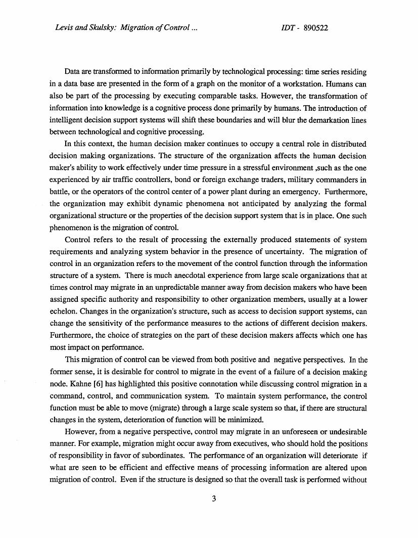
maker (DM) with bounded rationality [3]. There are four basic stages in the model, as illustrated in

the Petri Net of Figure 2.

5


voiSA C)IF CI RS

fl hl

x u v Y

Figure 2 Petri Net Model of the Interacting Decision Maker

Figure 2 Petri Net Model of the Interacting Decision Maker

• Situation Assessment (SA): In this stage, the DM receives an input x from the

environment and processes the information by using one of U algorithms fl,...,fu. Thefirst switch, a special transition that places a token in only one of its output places when it

fires, implements a decision rule p(u), which controls the choice of algorithm. The result of

the SA stage is z, the assessed situation At this stage, some information zio can betransmitted to the other organization members.

* Information Fusion (IF): The DM fuses his own situation assessment, z, with the

information he obtains from the rest of the organization, zoi. The revised assessment is z'.* Command Interpretation (CI): The DM may receive commands, vo i, from superiors

that restrict his options in the response selection stage.

* Response Selection (RS): Finally, a response Y is generated, which depends on the

assessed situation z'- and the choice of response selection algorithm.The decision strategy

associated with the switch is denoted p(v I z). The response Y can go to the environment

(output) or to other decision makers in the organization.

By interconnecting such models according to a prescribed set of rules [12] and by integrating

the models of the decision support systems, complete models of organizations are obtained [2]. To

carry out the analysis of such organizations requires defining measures of performance (MOPs)

such as accuracy, response time, workload, and degree of coordination. These MOPs can be

computed for different organizations using CAESAR (Computer Aided Evaluation of System

6


ARchitectures) a suite of algorithms and graphics tools designed and operated at the MIT

Laboratory for Information and Decision Systems (LIDS).

Organizations can be seen as systems performing specific missions. These missions involve

tasks with inputs xi which have discrete probability distribution Pr(xi ) and cost function C(y, Ydi).

Pr(xi) is the probability that the decision making organization (DMO) receives the input xi , and has

to perform the corresponding task, while C(y, Ydi) assigns a cost to each response to this task.

This is done by mapping x i into an ideal or desired response Ydi. Then, C(y,ydi) associates a

value to the discrepancy between the actual response y and the desired response. Within this

framework, an MOP which evaluates the organization's performance on a task can be introduced:

Measure of Performance, J, measures how well the response of the organization

corresponds to the desired response [1]. For each organizational strategy and each input,

the cost C is computed. Unless the algorithms used are deterministic, there is more than one

possible response for a given input xi . The value of J for a strategy S is:

J(6) = li p(xi) 1h C(y h,Ydi) P(Yh Ixi ) (1)

Strategies can be categorized as pure and mixed [4]. Pure internal strategies of the rth DM are

those for which both the situation assessment strategy p(u) and the response selection strategy

p(v I z) are pure. Pure means that one of the algorithms fi is selected with probability 1 and one of

the algorithms hj is selected with probability 1, when the situation assessment is z. Thus:

Dkr = {p(u = i) = 1; p(v =j I z = zm) = 1} (2)

for some i, j, and zm in the set Z. There are U algorithms f for situation assessment, and V

algorithms h for response selection. M is the dimension of the set Z. Therefore, for the rth

decision maker, there are nr possible pure strategies

nr = U (VM) (3)

The remaining internal strategies are the mixed strategies, which are convex combinations of pure

strategies:nr

Dr(Pk) = IPkDk (4)k=l

where

7


nr

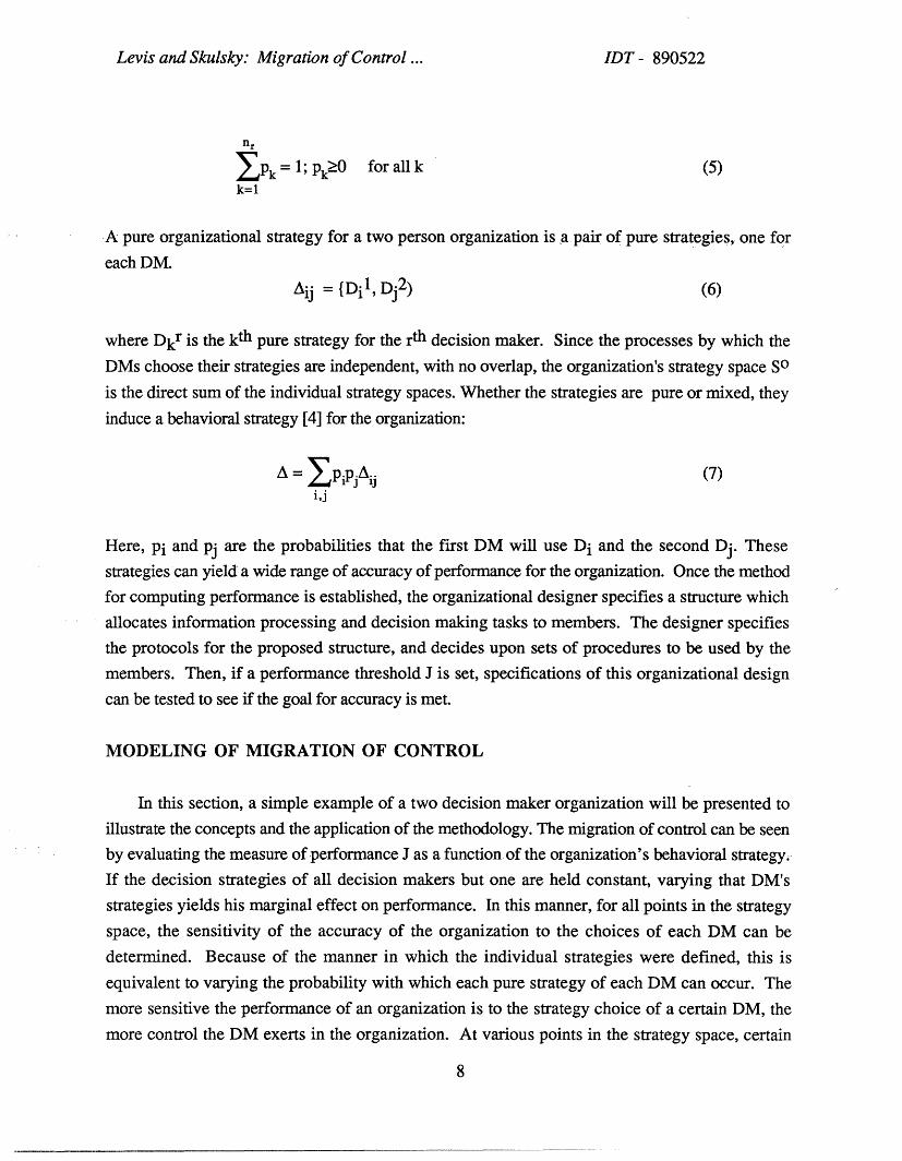
1Pk = 1; PkO0 for all k(5)k=l

A pure organizational strategy for a two person organization is a pair of pure strategies, one for

each DM.

Aij = {Dil, Dj 2 ) (6)

where Dkr is the kth pure strategy for the rth decision maker. Since the processes by which the

DMs choose their strategies are independent, with no overlap, the organization's strategy space SO

is the direct sum of the individual strategy spaces. Whether the strategies are pure or mixed, they

induce a behavioral strategy [4] for the organization:

A = jPiPjAij (7)1,j

Here, Pi and pj are the probabilities that the first DM will use D i and the second Dj. These

strategies can yield a wide range of accuracy of performance for the organization. Once the method

for computing performance is established, the organizational designer specifies a structure which

allocates information processing and decision making tasks to members. The designer specifies

the protocols for the proposed structure, and decides upon sets of procedures to be used by the

members. Then, if a performance threshold J is set, specifications of this organizational design

can be tested to see if the goal for accuracy is met.

MODELING OF MIGRATION OF CONTROL

In this section, a simple example of a two decision maker organization will be presented to

illustrate the concepts and the application of the methodology. The migration of control can be seen

by evaluating the measure of performance J as a function of the organization's behavioral strategy.

If the decision strategies of all decision makers but one are held constant, varying that DM's

strategies yields his marginal effect on performance. In this manner, for all points in the strategy

space, the sensitivity of the accuracy of the organization to the choices of each DM can be

determined. Because of the manner in which the individual strategies were defined, this is

equivalent to varying the probability with which each pure strategy of each DM can occur. The

more sensitive the performance of an organization is to the strategy choice of a certain DM, the

more control the DM exerts in the organization. At various points in the strategy space, certain

8


DMs may assume control and then yield control to others at other points, when the accuracy grows

less sensitive to their decisions. This is the phenomenon of migration of control.

Consider now the migration of control behavior in an organization consisting of two decision

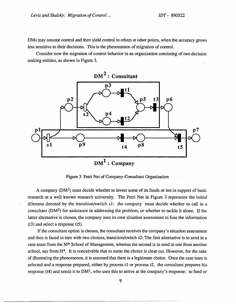
making entities, as shown in Figure 3.

DM 2 : Consultant

sl p9

SI p9 t4 p8 t5

DM 1 : Company

Figure 3 Petri Net of Company-Consultant Organization

A company (DM1) must decide whether to invest some of its funds or not in support of basic

research at a well known research university. The Petri Net in Figure 3 represents the initial

dilemma denoted by the transition/switch sl: the company must decide whether to call in a

consultant (DM2) for assistance in addressing the problem, or whether to tackle it alone. If the

latter alternative is chosen, the company uses its own situation assessment to fuse the information

(t3) and select a response (t5).

If the consultant option is chosen, the consultant receives the company's situation assessment

and then is faced in turn with two choices, transition/switch s2: The first alternative is to send in a

case team from the M* School of Management, whereas the second is to send in one from another

school, say from H*. It is conceivable that to some the choice is clear cut. However, for the sake

of illustrating the phenomenon, it is assumed that there is a legitimate choice. Once the case team is

selected and a response prepared, either by process tl or process t2, the consultant prepares his

response (t4) and sends it to DM 1, who uses this to arrive at the company's response: to fund or

9


not to fund university research.

To evaluate the measure of performance for this organization, one must know the values that

will result from the pure strategies outlined above. If the DM1 chooses to analyze the case alone,

the value of J will be 6 on a scale of 1 to 10, where the better the outcome the higher the value. If

the consultant is called in, the value of J will be 8 -if the case is handled by the capable M* team,

and 5 if by the H* team. Thus, the performance measure takes the form:

J = 6p + (1-p)[8q + 5(1-q)] = 5 + p +3q -3pq (8)

where p is the probability DM 1 will tackle the case alone and q is the probability that the M* team

will be used. This J value is based on the organizational strategy, and is a measure of the

closeness of the response yielded by this strategy to the ideal organizational response. A

three-dimensional graph of J versus p and q (Figure 4) shows where in the strategy space

performance is highest. One can see that in Figure 4, at (p, q) = (0, 0) where the consultant has

been called in and he selects the H* team with probability 1, the accuracy will be 5. As the

probability that the superior S* team will be put on the case is increased, as q is increased from 0

to 1, holding p fixed at 0, performance rises rapidly from 5 to 8. As the probability that the

company will handle the case alone increases, i.e., as p is increased to 1, holding q fixed at 0, J

rises to 6. Note that if p is set to unity, i.e., the company will handle the decision alone, the

decision by the consultant as to whether to use the M* or the H* team is irrelevant. This is shown

in Figure 4 by the constant value of J, at 6, for all values of q. One can also see graphically the

effect on performance of incremental changes in the DMs' strategies.

However, the ideal response changes with the inputs to the organization. Under different

conditions, different responses will be optimal. In this case, the inputs into the organization that

provide both DMs with the information they must consider in arriving at a decision are the students

and faculty at the research university. If the current staff is up to par, certainly the ideal response

would be to invest in university research. The sensitivity coefficient S 1 for the company is the

percentage change that will occur in J in response to a one percent change in the probability p that

characterizes the company's strategy. The sensitivity coefficient is defined as:

S J(Po (9)= J(Po, qo ) Op po , q0o

and is evaluated at the point (Po, qo) of the strategy space. Similarly, for the consultant's

10


sensitivity coefficient:

2,qO (10)

J(Po, qo) *q po, qO

6.00

Figure 4 Performance versus strategies for DM1 and DM2

A subscripted numeral represents the strategy number and a superscripted numeral represents

the DM number. To find J and the sensitivity coefficient S 1, q is set at zero, and p is varied from 0to 1; then q is incremented and again p is varied from 0 to 1. For S 2 , p is set at zero, and q is

varied from 0 to 1, then p is incremented and q is varied form 0 to 1. Sensitivity depends upon the

direction in which the derivative is taken as well as the point in the strategy space (Po, qO) for

which it is determined. Thus, at each point (po, qo), there are two sensitivity coefficients as

defined in equations (9) and (10). For this very simple case, the actual expressions for the

sensitivity coefficients can be derived:

S 1 = (1-3q) p / J

S 2 = 3(1-p)q/J (11)


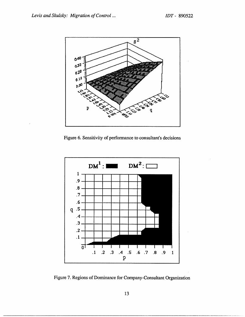
The two sensitivity coefficients have been plotted as functions of the two strategies, p and q, as

shown in Figures 5 and 6. By comparing these two plots, the regions in the strategy space where

a decision maker has more control over the decision making process of the organization relative to

the other DM are determined. The comparison is done on the basis of the absolute values of the

sensitivity coefficients:

If /S 1 / > /S2/, then DM1 is dominant; if/S2 / > IS1/, then DM2 is dominant.

A420

Figure 5. Sensitivity of performance to company's decisions

It is evident from the diagrams that DM1, the company, has most control on the situation when

(p, q) = (1, 0); that is, obviously, when the company handles the case alone. As p decreases,

control is passed to the consultant, because the latter's decision as to whether to select the M* or

the H* team has more impact on performance. Note, however, that if the consultant favors with

very high probability the H* team, the company may remain dominant. This occurs because the

difference in performance between the company arriving at a decision alone and using a consultant

with the H* team is smaller (from 5 to 6) than if the M* team is to be used (6 to 8). These results

are summarized in the strategy space where the regions of dominance are shown (Figure 7). The

shaded area shows for which points in the strategy space the company is dominant, while the

unshaded area shows the region where the consultant is dominant.

12


0.0

: q

Figure 6. Sensitivity of performance to consultant's decisions

DM 1 : DM2 E11

.9-

.7-

.6…-

.4- - -

.3

.1 .2 .3 .4 .5 .6 .7 .8 .9 1P

Figure 7. Regions of Dominance for Company-Consultant Organization

13


In this very simple case, each region of dominance is connected. The problem for the designeris to examine the boundary between the two regions and then to make modifications in theorganizational structure and its rules of operation so that the boundary will be shifted as needed.I nthe general case, however, the region of dominance of a decision maker can consist of a number ofdisjoint subregions. When the regions are disjoint, the problem is more complex both in terms of

understanding the dynamics of the organization (the mental models of its operation by the decision

makers themselves may be too simplistic or incorrect) and in terms of organization redesign. Such

a case is discussed in the following section.

MIGRATION OF CONTROL IN N-OPTION DECISION MAKINGORGANIZATIONS

This example of a two decision maker organization with a mission to detect enemy submarines

was studied from the standpoint of coordinating the decision makers' activities by Grevet [5]. Thetwo entities are a submarine (DM 1) and a surface ship (DM2). The Petri Net model for this

organization is depicted in Figure 8.

29 CI RS

(,4

DM2

Figure 8. Two Decision Maker Organization Aided by Decision Support System

14


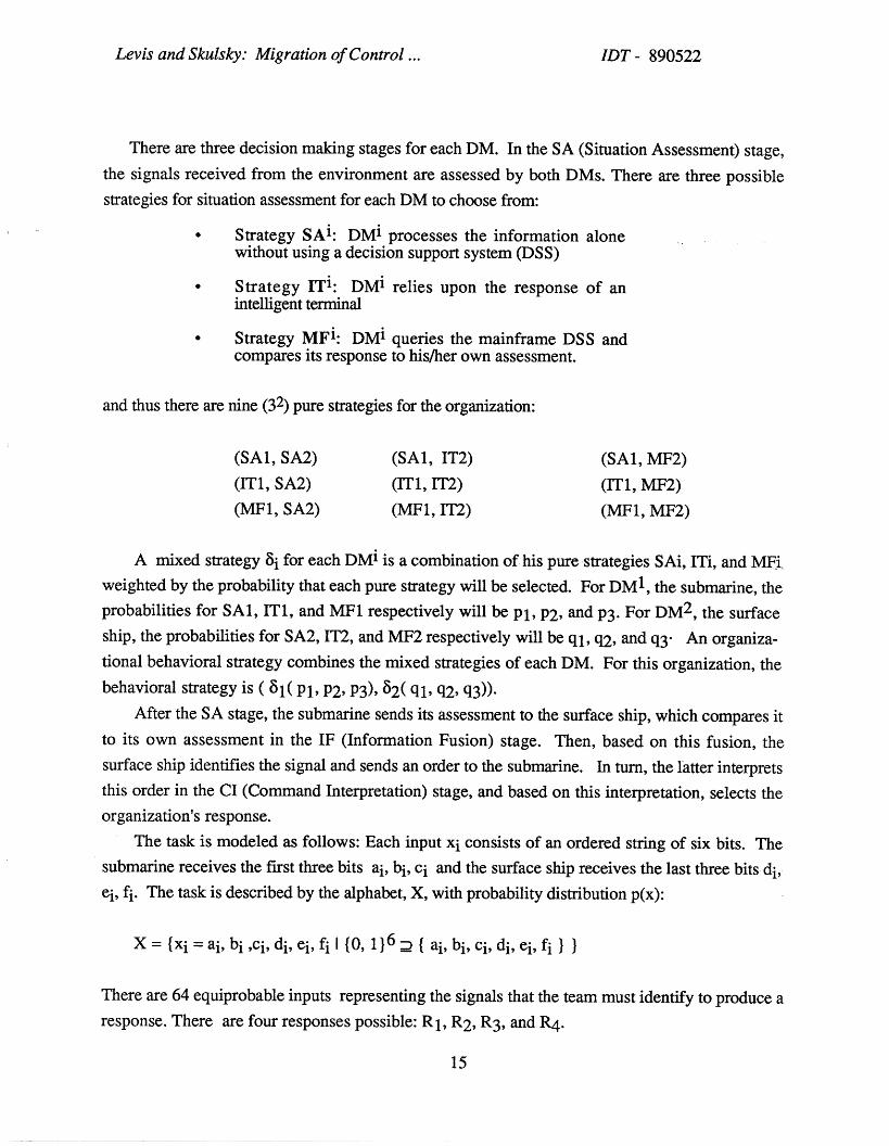
There are three decision making stages for each DM. In the SA (Situation Assessment) stage,the signals received from the environment are assessed by both DMs. There are three possiblestrategies for situation assessment for each DM to choose from:

* Strategy SAi: DMi processes the information alonewithout using a decision support system (DSS)

* Strategy ITi: DMi relies upon the response of anintelligent terminal

* Strategy MFi: DMi queries the mainframe DSS andcompares its response to his/her own assessment.

and thus there are nine (32) pure strategies for the organization:

(SA1, SA2) (SA1, IT2) (SA1, MF2)(IT1, SA2) (IT1, IT2) (IT1, MF2)(MF1, SA2) (MF1, IT2) (MF1, MF2)

A mixed strategy §i for each DMi is a combination of his pure -strategies SAi, ITi, and MFiRweighted by the probability that each pure strategy will be selected. For DM 1, the submarine, theprobabilities for SA1, IT1, and MF1 respectively will be Pl, P2, and p3. For DM2 , the surfaceship, the probabilities for SA2, IT2, and MF2 respectively will be ql, q2, and q3- An organiza-tional behavioral strategy combines the mixed strategies of each DM. For this organization, the

behavioral strategy is ( 61( Pl, P2, P3), 82( ql, q2, q3)).After the SA stage, the submarine sends its assessment to the surface ship, which compares it

to its own assessment in the IF (Information Fusion) stage. Then, based on this fusion, thesurface ship identifies the signal and sends an order to the submarine. In turn, the latter interpretsthis order in the CI (Command Interpretation) stage, and based on this interpretation, selects theorganization's response.

The task is modeled as follows: Each input x i consists of an ordered string of six bits. Thesubmarine receives the first three bits ai, bi, ci and the surface ship receives the last three bits di,ei, fi. The task is described by the alphabet, X, with probability distribution p(x):

X = {xi = ai , b i ,ci, di, ei, fi I {0, 1}6 { ( ai , bi, ci, di, ei, fi } }

There are 64 equiprobable inputs representing the signals that the team must identify to produce aresponse. There are four responses possible: R1 , R 2, R 3 , and R 4 .

15


* CASE 1: If bits ai and di both equal 0, the signal is not from anenemy sub, and the submarine should not counteract. This responseis R 1, and the probability of the corresponding input is 1/4.

* CASE 2: If case 1 does not hold and bits bi and ei both equal 0,(input probability 3/16) the signal comes from an enemy sub testingsubmarine DM 1. Here, DM 1 should confuse the enemy sub byunder reacting (response of R2 .)

* CASE 3: If cases 1 and 2 do not hold and bits ci and fi equal 0, amoderately threatening enemy submarine is present. DM 1 should over-react, to deter the enemy. This response is R 3, and the probability ofthe corresponding input is 9/64.

* CASE 4: If none of the above cases hold, then the signal comesfrom an enemy submarine which is threatening DM 1. Now, thesubmarine DM1 should over-react more forcefully than in case 3. Thisinput probability is 27/64. The response is R4.

The cost matrix giving the costs associated with the discrepancies between the actual and idealresponses is shown in Table 1.

TABLE 1: Cost Matrix

actual

ideal R1 R2 R3 R4

R1 0 2 3 4

R2 4 0 1 2

R3 6 4 0 2

R4 8 4 3 0

The different strategies vary in effectiveness of processing information. When the DMs

assess the input without the DSS, they identify correctly the first two of their three bits.Therefore, for an input xi = (ai, bi, ci, di, ei, fi), the result of the situation assessment when DM1

16


uses the SA strategy is (a i, b i, ui) where ui is what DM 1 produces as the value for the third bit.

This value has a probability of 0.5 of being equal to c i (the actual value). Similarly, for DM2, the

result is (di, ei, vi) where v i is equal to fi with probability 0.5. When the IT strategy is used, the

first bit of each DM's three bits is identified correctly all the time, while the other two are identified

correctly with probability 0.5. And for the MF strategy, all bits are identified correctly all the time.

Thus, the organization is guaranteed to perform correctly at all times only if the organizational

strategy is (MF1, MF2). The performance measure J for this organization is the expected value of

the cost for not identifying the string xi correctly, i.e., inaccuracy, and is obtained by multiplying

the cost of each pure strategy by the probability of its occurrence:

rqllJ [P1 P2 P3] J I q2 1

L q3where

Jll J2 J 13 1 .53.98 .351J= 21 J22 J23 1= .98 1.2 .831 (12)

LJ3 1 J32 J33 L .35 .83 0

Note that up to the situation assessment phase, the two DM's actions and options are identical:

they operate in parallel. Thus, the J matrix is symmetric. Furthermore, since in the (MF1,MF2)

case the costs are zero, the corresponding term in the J matrix is also zero.

When analyzing migration of control in the consultant-client case, only one parameter was

needed to characterize the strategy of each DM, since their choices were binary. Here, however,

each switch has three branches indicating three options. However, since the parameters

characterizing the points in the strategy space are probabilities, the 3-option case can be expressed

in terms of 2 parameters, as shown in equation (13).

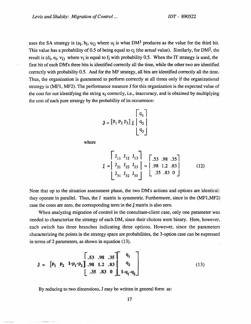
r.53 .98 .35 q1J = [Pi P2 1-Pl-P21 .98 1.2 .83 2 (13)

L .35 .83 0 IL-q 1-q 2J

By reducing to two dimensions, J may be written in general form as:

17


= [P1 P2] [ 7 -.2 46 q2 1+ [.35 .831 PI+ [.35 .8311 +const. (14)-2 .462 [2 LP21 Lq2 j

In this case, the constant is zero because of the zero value of J33 . The sensitivity coefficients for

each DM are defined as follows:

S1= [Pl/J P2/J] 1 S2 = 1[ql/J QJ] j1 (15)

[4P2s [lq2

Again, in this case, a closed form expression can be obtained for the two sensitivities:

S-l [PlIJ /J] - 0.17q - 0.2q + 0.350.2q1 - 0.46q2 + 0.83

2 [q /j q2/J] [0.17p, - 0.2p 2 + 0.351o - (16)S ii 0.2p1 - 0.4 6 P2 + 0.83]

where J is as defined in equation (14). At this point, the calculations can be done efficiently using

a spreadsheet; the values for the sensitivity coefficient for each DM at all points in the strategy

space can be determined and plotted as a function of the strategies (Pl, P2) and (ql, q2).

The computations for the antisubmarine warfare case, with three options, can be easily

extended analytically to the n-option case with a reduction; however, the graphical representation of

the regions of dominance becomes much more complex.

Given the versatility of spreadsheet software for the MacintoshT M , there are many formats in

which to analyze the migration of control. Each reveals a different perspective of how the structure

of an organization impact on the relative control of its members. The various plots that can be

made include:

18


· The sensitivity coefficient for each DM is obtained as a function of the organization's

behavioral strategies. That requires to plot a surface in the five-dimensional space: S vs

(Pi, P2, q 1, q2). One way to accomplish that is discretize the two- dimensional strategyspace of each DM in terms of a rectangular grid and t hen order -the pairs. Then a three-.

dimensional plot, a surface, can be obtained of S vs. ( P, P2) and (ql, q2 ).

* The regions of dominance for each DM in the four dimensional behavioral strategy space.Again, in this case, if the discretization of the strategy space is carried out, including theordering of the pairs, a two dimensional strategy space is obtained in which the regions of

dominance can be depicted. Note, however, that the manner in which the pairs ( Pi, P2)and (ql, q2 ) are ordered will affect the appearance of the regions.

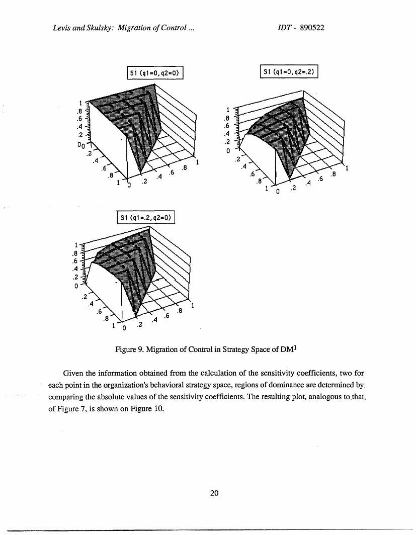
Of course, it is always possible to parametrize the strategy space and plot the sensitivity due toone DMs changes in strategies for a fixed strategy of the other DM. For example, observing howS1 varies in the strategy space of DM 1 for incremental changes in the DM2 's strategies provides

some interesting insights on the effect on control of using a less efficient strategy.

As illustrated in Figure 9, where both ql and q2 equal zero, the strategy choice of DM2 being

querying the mainframe, results in perfect accuracy on his part. Therefore, the performance

measure is most sensitive to the decisions of DM1 throughout his entire strategy space (exceptwhen P1 and P2 are also both zero). DM 1 gains control, shown by a larger sensitivity coefficient

S1 , as P1 and P2 increase, and loses control as ql and q2 increase. This can be observed in theshaded areas of the plots, in which Pi + P2 < 1. Strategy 1, assessing the situation without aid,SA1, and 2, using the intelligent terminal, IT1, yield larger values of J (and thus worse accuracy)

than strategy 3, querying the mainframe, MF1. Therefore, increased likelihood of a DM usingeither of the two less effective strategies has more effect on accuracy than increased likelihood ofthe DM using strategy 3. This is intuitively appealing: when performance is very poor, smallchanges can yield substantial performance improvements. Thus, the actions of DM1 when P1 and

P2 are large have greater impact than when p3 is large. The fact that strategy 2 is the least effectiveexplains why. In the plots where either ql or q2 is nonzero, the S1 surface slopes gently upwardas pi is increased, and rises more dramatically-when P2 is increased. Comparison of the three plotsin Figure 9 shows that, when ql and q2 are large, DM2 gains control just as DM1 does when Piand P2 are large. And since there are only two DMs, when one DM dominates, the other recedes.

19


si (ql=O,q2=0) S1 (ql=O,q2=.2)

.8 1!BI5P ~

.6 .8

.4 .6.2 .4

O0

.4 =.2,

.8

.4.6 .

0

Figure 9. Migration of Control in Strategy Space of DM

Figure 9. Migration o f Control in Strategy Space of DM 1

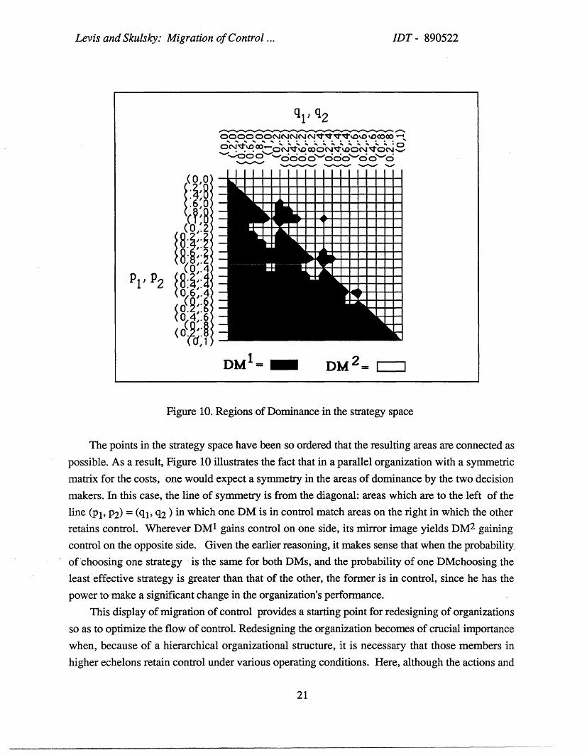
Given the information obtained from the calculation of the sensitivity coefficients, two for

each point in the organization's behavioral strategy space, regions of dominance are determined by_

comparing the absolute values of the sensitivity coefficients. The resulting plot, analogous to that..

of Figure 7, is shown on Figure 10.

20


ql' q20000 ooNNNsNN t 'd O >Dazoo

oo n 0 "zoooqtl otl00 00

(O,.6,0

<7 2DM DM = -

Figure 10. Regions of Dominance in the strategy space

The points in the strategy space have been so ordered that the resulting areas are connected as

possible. As a result, Figure 10 illustrates the fact that in a parallel organization with a symmetric

matrix for the costs, one would expect a symmetry in the areas of dominance by the two decision

makers. In this case, the line of symmetry is from the diagonal: areas which are to the left of the

line (PI, P2) = (q1, q2 ) in which one DM is in control match areas on the right in which the other

retains control. Wherever DM 1 gains control on one side, its mirror image yields DM 2 gaining

control on the opposite side. Given the earlier reasoning, it makes sense that when the probability

of choosing one strategy is the same for both DMs, and the probability of one DMchoosing the

least effective strategy is greater than that of the other, the former is in control, since he has the

power to make a significant change in the organization's performance.

This display of migration of control provides a starting point for redesigning of organizations

so as to optimize the flow of control. Redesigning the organization becomes of crucial importance

when, because of a hierarchical organizational structure, it is necessary that those members in

higher echelons retain control under various operating conditions. Here, although the actions and

21


options of the DMs are identical up to their situation assessment stage, the organization is

hierarchical. The submarine DM 1, the subordinate, will send the result of its assessment to the

commander, DM2, who will fuse this with its own assessment, identify the signal, and produce a

directive which is sent to the subordinate. In turn, the subordinate interprets this order, and

produces the organizational response. However, the situation as analyzed. reveals no such

hierarchy. Therefore, it is desirable to redesign the concept of operations so that DM2 retains

control in most cases.

It is possible to develop rules for redesigning the organization for specific operating

conditions. For example, suppose that DM2 , the commander, finds that although not as accurate

as the other assessment alternatives, the intelligent terminal (IT) provides better performance with

respect to speed and ease of use, and so he decides to choose this alternative, strategy IT2, at all

times. Then, q2 = 1. This structure preserves the commander's control: for every mixed strategy

of the submarine, DM1, the commander DM2 retains control.

CONCLUSION

A methodology, and the associated models, have been described that allow designers of

information processing and decision systems to investigate the effect their designs have on the

properties of decision making organizations. Specifically, a quantitative model of a property that

becomes very important when distributed decision making is considered, the migration of control,

has been described and illustrated with application to two simple examples. The concepts used and

the computational procedures presented are not limited to simple examples; they apply to arbitrary

size organizations. The depiction of the complete results in simple graphs depends, however, on

the dimensionality of the problem; use of the specific features of individual problems may help

reduce the dimensionality of the strategy space, as was illustrated with the second example. This

work is continuing, as part of an effort to understand the dynamics of organizations that function

through the use of decision support systems.

REFERENCES

[1] S. K. Andreadakis and A. H. Levis, Accuracy and timeliness in decision makingorganizations. Proc. 10th IFAC World Congress (Pergamon Press, Oxford, 1987).

[2] S. K. Andreadakis and A. H. Levis, Synthesis of distributed command and control forthe outer air battle. Proc. 1988 Symposium on C2 Research (SAIC, McLean, VA,1988)

22


[3] K. L. Boettcher and A. H. Levis, Modeling the interacting decision maker withbounded rationality. IEEE Transactions on Systems, Man, and Cybernetics, SMC-120(3) (1982) 334-344.

[4] K. L. Boettcher and A. H. Levis, Modeling and Analysis of Teams of InteractingDecisionmakers with Bounded Rationality," Automatica, Vol. 19, No. 6, pp. 703-709,1983.

[5] J. L. Grevet, Decision Aiding and Coordination in Decision-Making Organizations,MS Thesis, Laboratory for Information and Decision Systems, MIT, ReportLIDS-TH-1737, (1988).

[6] S. Kahne, Control Migration: A Characteristic of C3 Systems, IEEE Control SystemsMagazine, 3 (1) (1983) 15-19.

[7] J. S. Lawson, Jr., Command control as a process. Control Systems Magazine 1 (1)(1981) 5-11.

[8] A. H. Levis, Information Processing and Decision-Making Organizations: aMathematical Description, Large Scale Systems, 7, (1984) 151-163.

[9] A. H. Levis and M. Athans, The quest for C3 theory: dreams and realities, in S. E.Johnson and A. H. Levis (Eds.), The Science of Command and Control: Coping withUncertainty (AFCEA, Fairfax, VA, 1988).

[10] A. A. Louvet, J. T. Casey and A. H. Levis,Experimental investigation of the boundedrationality constraint, in S. E. Johnson and A. H. Levis (Eds.), The Science ofCommand and Control: Coping with Uncertainty (AFCEA, Fairfax, VA, 1988).

[11] W. Reisig, Petri Nets: An Introduction (Springer-Verlag, Berlin, 1985).

[12] P. A. Remy and A. H. Levis, On the generation of organizational architectures usingPetri Nets, in: G. Rozenberg (Ed.), Advances in Petri Nets 1988 (Springer-Verlag,Berlin, 1988).

[13] M. Van Creveld, Command in War (Harvard University Press, Cambridge, MA,1985).

23

MIGRATION OF CONTROL IN DECISION MAKING ORGANIZATIONS 1

Documents

Transcript of MIGRATION OF CONTROL IN DECISION MAKING ORGANIZATIONS 1