Migration and inversion of seismic datamosrp.uh.edu/content/07-news/papers-videos-where... ·...
15
GEOPHYSICS, VOL. 50, NO. 12 (DECEMBER 1985); P. 2458-2472, 1 TABLE. Migration and inversion of seismic data R. H. Stolt* and A. B. Wegleint ABSTRACT Seismic migration and inversion describe a class of closely related processes sharing common objectives and underlying physical principles. These processes range in complexity from the simple NMO-stack to the complex, iterative, multidimensional, prestack, nonlin- ear inversion used in the elastic seismic case. By making use of amplitudes versus offset, it is, in principle, possible to determine the three elastic param- eters from compressional data. NMO-stack can be modified to solve for these parameters, as can pres tack migrl).t ion. Linearized, wave-equation inversion does not inordi- nately increase the complexity of data processing. The principal part of a migration-inversion algorithm is the migration. Practical difficulties are considerable, including both correctable and intrinsic limitations in data quality, limitations in current algorithms (which we hope are correctable), and correctable (or perhaps intrinsic) limi- tations in computer power. INTRODUCTION The words "migration" and "inversion" are, in fact, used to describe a number of related processes. To some people, seis- mic migration is strictly an imaging process. To others, seismic data already form an image which needs only to be massaged, or "migrated," into its proper location. To still others, migra- tion is an inversion process which derives two-dimensional (or three-dimensional) maps of local reflectivity from seismic data. Notions of seismic inversion are even more diverse, mainly because several inverse problems (and several approaches to solve them) can be formulated for seismic data. Traveltime information can be inverted for seismic velocities using "veloc- ity analysis" or, for near-surface variations using "statics." A single stacked common-midpoint (CMP) trace forms an esti- mate of local reflectivity which, when combined with low- frequency velocity information (from well logs or velocity analysis), can be time-integrated to form an impedance esti- Manuscript reviewed by Norman Bleistein. mate. This process is sometimes referred to as inversion (Lind- seth, 1979). More rigorous (and we hope, more realistic inver- sion) methods based on wave-equation analysis can also ex- tract information from traveltimes and reflectivities. The exact one-dimensional (I-D) acoustic inverse problem for plane waves at normal incidence has been vigorously at- tacked, solving, at least on paper, for absolute values of acous- tic impedance (e.g., Goupillaud, 1961; Ware and Aki, 1969; Berryman and Greene, 1980; Howard, 1983). Plane waves at nonnormal incidence have also been addressed with individual solutions for velocity and density (e.g., Stolt and Jacobs, 1980; Coen, 1981 and 1982; Hooshyar and Razavy, 1983). The in- verse acoustic linearized problem has been solved for point sources and receivers (Raz, 1981a, b). The inverse problem for elastic waves has also been approached, both by linearized approximation (Clayton, 1981) and through iterative modeling (McAulay, 1985). Some of the point-source methods (e.g., McAulay, 1985) use traveltime as well as reflectivity infor- mation. Others (e.g., Clayton, 1981) assume travel times are known a priori and analyze only reflectivity information. One- dimensional processing (based on the wave equation) of CMP gathers can, on the one hand, be viewed as a restriction of the general migration or inversion problem and, on the other hand, as an extension of conventional processing and single- trace inversion methods. The relevance of all these solutions to the real seismic problem has not always been clear. The real Earth is certainly not acoustic, nor exactly elastic, and it cer- tainly is not exactly one-dimensional. Considerable research has been concentrated on multidi- mensional wave-equation inversion, beginning with Cohen and Bleistein (1977). Mostly, the treatment has been in the linear approximation, ignoring transmission losses and multi- ple reflections, though approaches to full iterative solutions have appeared in the literature (Tarantola, 19"84). Approaches to both many-offset (Clayton and Stolt, 1981; Raz, 1981a, b) and zero-offset (Bleistein and Cohen, 1979 and 1982) data have been considered. Zero-offset inversion relates easily to poststack migration. Multidimensional migration and wave-equation inversion differ more in emphasis than in substance (migration is pre- occupied with propagation, inversion with reflection or scat- tering), and approach essentially the same problem from Manuscript received by the Editor March 5, 1985; revised manuscript received April 30, 1985. *Conoco Inc. Exploration Research Division, P. O. Box 1267, Ponca City, OK 74603. :j:Sohio Petroleum Co., Technology Center, Geophysical R&D, One Lincoln Center, Dallas, IX 75240. CD 1985 Society of Exploration Geophysicists. All rights reserved. 2458 Downloaded 04/16/13 to 129.7.16.11. Redistribution subject to SEG license or copyright; see Terms of Use at http://library.seg.org/
-
Upload
truongdung -
Category
Documents
-
view
227 -
download
1
Transcript of Migration and inversion of seismic datamosrp.uh.edu/content/07-news/papers-videos-where... ·...
GEOPHYSICS, VOL. 50, NO. 12 (DECEMBER 1985); P. 2458-2472, 1 TABLE.
Migration and inversion of seismic data
R. H. Stolt* and A. B. Wegleint
ABSTRACT
Seismic migration and inversion describe a class of closely related processes sharing common objectives and underlying physical principles. These processes range in complexity from the simple NMO-stack to the complex, iterative, multidimensional, prestack, nonlinear inversion used in the elastic seismic case.
By making use of amplitudes versus offset, it is, in principle, possible to determine the three elastic parameters from compressional data. NMO-stack can be modified to solve for these parameters, as can pres tack migrl).tion.
Linearized, wave-equation inversion does not inordinately increase the complexity of data processing. The principal part of a migration-inversion algorithm is the migration.
Practical difficulties are considerable, including both correctable and intrinsic limitations in data quality, limitations in current algorithms (which we hope are correctable), and correctable (or perhaps intrinsic) limitations in computer power.
INTRODUCTION
The words "migration" and "inversion" are, in fact, used to describe a number of related processes. To some people, seismic migration is strictly an imaging process. To others, seismic data already form an image which needs only to be massaged, or "migrated," into its proper location. To still others, migration is an inversion process which derives two-dimensional (or three-dimensional) maps of local reflectivity from seismic data.
Notions of seismic inversion are even more diverse, mainly because several inverse problems (and several approaches to solve them) can be formulated for seismic data. Traveltime information can be inverted for seismic velocities using "velocity analysis" or, for near-surface variations using "statics." A single stacked common-midpoint (CMP) trace forms an estimate of local reflectivity which, when combined with lowfrequency velocity information (from well logs or velocity analysis), can be time-integrated to form an impedance esti-
Manuscript reviewed by Norman Bleistein.
mate. This process is sometimes referred to as inversion (Lindseth, 1979). More rigorous (and we hope, more realistic inversion) methods based on wave-equation analysis can also extract information from traveltimes and reflectivities.
The exact one-dimensional (I-D) acoustic inverse problem for plane waves at normal incidence has been vigorously attacked, solving, at least on paper, for absolute values of acoustic impedance (e.g., Goupillaud, 1961; Ware and Aki, 1969; Berryman and Greene, 1980; Howard, 1983). Plane waves at nonnormal incidence have also been addressed with individual solutions for velocity and density (e.g., Stolt and Jacobs, 1980; Coen, 1981 and 1982; Hooshyar and Razavy, 1983). The inverse acoustic linearized problem has been solved for point sources and receivers (Raz, 1981a, b). The inverse problem for elastic waves has also been approached, both by linearized approximation (Clayton, 1981) and through iterative modeling (McAulay, 1985). Some of the point-source methods (e.g., McAulay, 1985) use traveltime as well as reflectivity information. Others (e.g., Clayton, 1981) assume travel times are known a priori and analyze only reflectivity information. Onedimensional processing (based on the wave equation) of CMP gathers can, on the one hand, be viewed as a restriction of the general migration or inversion problem and, on the other hand, as an extension of conventional processing and singletrace inversion methods. The relevance of all these solutions to the real seismic problem has not always been clear. The real Earth is certainly not acoustic, nor exactly elastic, and it certainly is not exactly one-dimensional.
Considerable research has been concentrated on multidimensional wave-equation inversion, beginning with Cohen and Bleistein (1977). Mostly, the treatment has been in the linear approximation, ignoring transmission losses and multiple reflections, though approaches to full iterative solutions have appeared in the literature (Tarantola, 19"84). Approaches to both many-offset (Clayton and Stolt, 1981; Raz, 1981a, b) and zero-offset (Bleistein and Cohen, 1979 and 1982) data have been considered.
Zero-offset inversion relates easily to poststack migration. Multidimensional migration and wave-equation inversion differ more in emphasis than in substance (migration is preoccupied with propagation, inversion with reflection or scattering), and approach essentially the same problem from
Manuscript received by the Editor March 5, 1985; revised manuscript received April 30, 1985. *Conoco Inc. Exploration Research Division, P. O. Box 1267, Ponca City, OK 74603. :j:Sohio Petroleum Co., Technology Center, Geophysical R&D, One Lincoln Center, Dallas, IX 75240. CD 1985 Society of Exploration Geophysicists. All rights reserved.
2458
Dow
nloa
ded
04/1
6/13
to 1
29.7
.16.
11. R
edis
trib
utio
n su
bjec
t to
SEG
lice
nse
or c
opyr
ight
; see
Ter
ms
of U
se a
t http
://lib
rary
.seg
.org
/
Migration and Inversion 2459
slightly different points of view. Papers describing the waveequation migration/wave-equation inversion relationship include Phinney and Frazer (1978), Bleistein and Cohen (1982), Clayton and Stolt (1981), Weglein (1982a, b), Berkhout (1984), and Cheng and Coen (1984).
Many-offset inversion relates to pres tack migration and combines elements of I-D prestack inversion and poststack migration or inversion (Weglein and Wolf, 1985; Stolt and Benson, 1985). Indeed, wave-equation prestack migration can be considered a form of prestack inversion which solves for only one of the three elastic parameters.
A comprehensive treatment of the many forms of migration and inversion is far beyond the scope of this paper. We only suggest that wave-equation inversion provides a unifying conceptual framework in which other approaches may be understood and also provides the potential of moving substantially beyond present-day capabilities of seismic processing and analysis. Table 1 lists methods of seismic processing and analysis and the wave-equation inversion procedure to which each corresponds or from which it can be derived.
Here we first describe a wave-equation linearized inverse for the three elastic parameters in a vertically changing earth. We then discuss realistic objectives for the inversion process, address migration and multidimensional linearized inversion, and briefly discuss nonlinear methods.
THE ONE-DIMENSIONAL INVERSE PROBLEM
There is a close relationship between CMP NMO-stack processing and I-D migration and inversion. CMP acquisition and processing rely on a ray-theoretical model, whereas migration and inversion tend to appeal directly to the wave equation. However, for frequencies and distances germane to seismic wave propagation, the geometrical (ray-theoretical) limit normally applies. This ensures at least a broad consistency between NMO-stack and conceptually deeper waveequation inversion processes.
We can easily note the essential similarity between NMOstack and a prestack Kirchhoff migration for a horizontally layered earth. It is also well-known that NMO-stack can be duplicated by an f-k dipless prestack migration (which is just NMO-stack inf-k space). Thus NMO-stack is, in its sphere, a legitimate process and is remarkably robust. In dealing with stacked data, even gross oversimplification often leads to useful results. For some applications, we can treat a stacked seismic trace as the result of a plane-wave experiment. This use (or abuse) of an obviously incorrect physical model is closely related to use of migration's exploding reflector model. It works well for primary reflections, provided locations are of more interest than amplitudes. Even amplitude problems can, to some extent, be patched up through minor modifications to the data. The final breakdown of the plane-wave model occurs when we try to incorporate multiple reflections. For that, the stacked seismic trace simply cannot be considered a plane wave.
Here, we layout a simple physical model for primary reflections of compressional waves in an elastic, layered earth. We begin with the wave-theoretical model of seismic inversion and relate it to the conventional ray-theoretical model. The result is an inversion algorithm which amounts to a move out correction and a weighted CMP stack. In principle, we can solve for each of the three elastic parameters (density, P veloc-
ity, and S velocity) by varying the weighting coefficients in the stack. Since this model ignores such niceties as multiple reflections and converted waves, it can only be viewed as incomplete. The relevance to exploration geophysics of an inverse to the 1-D elastic problem may be debatable, but it is not likely that the real Earth problem will be solved before this one.
The plane-wave reflection response
We begin with a simple stratified earth model characterized by the three elastic parameters:
a = compressional velocity,
~ = shear velocity, and
p = density.
We pass a plane compressional wave down through this model earth (assuming perfect transmission), collect the total up going compressional primary reflection response, and return it to the surface. Although our ultimate interest is in localized sources and receivers, we begin with plane waves, confident (e.g., Treitel et aI., 1982) that once we have one solution, we can find the other. It may seem a little odd (not to mention unnecessary) to include shear velocity in this model when our stated interest is in the compressional waves. In fact, the three elastic parameters constitute the minimum amount of realism necessary to describe the angular dependence of the reflection coefficients. The shear velocity is unnecessary to describe the transmission process, because we neglect compressional-to-shear conversion in the transmitted wave.
The appropriate downgoing wave is described by the WKBJ approximation (Morse and Feshbach, 1953). Consider a plane wave P of frequency (0 and ray parameter
p = sin e(z)/a(z), (1)
where e(z) is the angle the wave makes with the vertical at depth z. In the WKBJ approximation, this wave has the form
Jp(Z)U(Z) cos e(O) P(p, z, (0) = P(p, 0, (0) p(O)a(O) cos e(z)
x exp [i(o rz dz' cos e(l)]. Jo u(z')
(2)
The WKBJ approximation is the solution to the acoustic wave equation
(p ~ ~ ~ + (02 cos2 e) P = 0
dz p dz a 2
in the limit of high frequencies. At lower frequencies, it neglects reflected energy, converted energy, and transmission losses. The z dependence of P is contained in both the rapidly varying phase term and the relatively slowly varying amplitude term. The more important phase term depends upon velocity a, but not density p. The amplitude term depends upon both. It does not compensate for transmission losses but, rather, conserves energy as acoustic properties change.
If we were to change variables from depth to traveltime via
iz dz'
't = - cos e(z'), o a(z')
and from P to <1>, where
(3)
Dow
nloa
ded
04/1
6/13
to 1
29.7
.16.
11. R
edis
trib
utio
n su
bjec
t to
SEG
lice
nse
or c
opyr
ight
; see
Ter
ms
of U
se a
t http
://lib
rary
.seg
.org
/

2460
with
<j> = TIP,
TI=Jcose, pa
Stolt and Weglein
(4)
where (5)
[:t22 + ro2 - V(t)] <j>(p, t, ro) = 0, (7)
(8)
then in the new coordinate system the WKBJ approximation would become the simple plane wave
In this coordinate system the WKBJ approximation amounts to neglect of the potential term V(t). It is thus a first approximation in a Born-series expansion of the exact solution to the 1-D problem.
<j>(p, t, ro) = <j>(p, 0, ro)e i"". (6)
The wave equation in this coordinate system is (Jacobs and Stolt, 1980; Coen, 1981)
Having accepted the WKBJ approximation as an adequate description of transmission, we now need a reflection model.
Thble 1. Aspects of the inverse seismic problem.
Seismic processing and analysis methods
Wave equation inversion
One-dimensional Traveltime velocity One-dimensional inversion with offset in the geometric acoustics limit (WKBJ)
Two- and threedimensional
analysis
CMP stacked trace + Trace integration
Goupillaud equal traveltime inversion
Picking + Reflectivity estimates + Amplitude/offset
Picking + Reflectivity estimates + Amplitude/offset
Post- and prestack migration
Depth migration
Elastic migration Three-component
migration
Plane-wave, normalincident, singleparameter linearized inversion
Plane-wave, normalincident, singleparameter exact inversion
One-dimensional multiparameter (acoustic or elastic) linearized inversion with offset data)
Exact one-dimensional multiparameter inversion with offset data
Post- and prestack linear single-parameter inversion
Variable-background linearized inversion
Elastic linear inversion to find reflectivity
Depth migration with Nonlinear (exact) in-built velocity constant-density analysis and multiple acoustic inversion removal
Iterative, nonlinear, variable-density acoustic and elastic inversion
Dow
nloa
ded
04/1
6/13
to 1
29.7
.16.
11. R
edis
trib
utio
n su
bjec
t to
SEG
lice
nse
or c
opyr
ight
; see
Ter
ms
of U
se a
t http
://lib
rary
.seg
.org
/
Seismic Data Processing 2461
We divide the model earth into a large number of layers, each thin enough that the elastic parameters can be considered constant within each layer and that they will exhibit only small changes from one layer to the next. (This may require a much finer discretization than the data we eventually want to describe. The layers are not meant to be thought of as a discretization interval for processing, but as a conceptual tool.)
Depth to the bottom of the t'th layer is Zt, and thickness of the layer will be Ilz t = Zt - Zt _ 1. Elastic properties in this layer are U(, ~(' and Pt. At the bottom of the t'th layer, the incident wave is
JPtUt cos ao Pj(p, Zt, 0) = Pj(p, 0, 0) a
Po Uo cos t
x exp [iO) I Ilz(, cos at, jUt']· (9) t/~t
The compressional wave reflected from the layer bottom is, at z(, just the incident wave in equation (9) multiplied by a reflection coefficient:
Prt (p, Zt, 0) = P j (p, z(, O)R( (a t )llz(. (10)
The reflection coefficient per layer Rt depends upon the angle of incidence a( of the plane wave in the t'th layer. This angle obeys
(11)
For the reflection coefficient R(, we invoke Chapter 5 of Aki and Richards (1979). The exact Zoeppritz reflection coefficient is rather involved and unnecessarily complicated for small changes between adjacent layers. Consequently, we borrow an approximate expression [Aki and Richards, equation (5.44)]
1 ( ~;. 2 ) dp( 1 2 dUt Rt(at ) ~ - 1 - 4""2 sm at -- + - sec at --2 Ut Pt Ilzt 2 Ut Ilzt
~ . 2a Il~ ) -4""2sm t~. (12 Ut PtLlZt
The main benefit of choosing the expression (12) over an exact reflection coefficient is that expression (12) is linear in fractional changes of the elastic parameters. This simplifies the expression not only conceptually [just looking at expression (12), we easily see the effect of individual parameter changes], but computationally (the result is not sensitive to errors in absolute amplitude). Validity of expression (12) requires not only that changes at the layer boundary be small, but also that at not approach critical angle.
Given an expression for Rt , it remains to sum contributions from all layers and propagate them to the surface. The result is
P.(p, 0, 0) = Pj (p, 0, 0) I Ilzt Rt (at) t
x exp [2iO) I Ilzt, cos at, jUt']· (13) t''''t
When the largest layer thickness dZt is forced to zero, equation (13) becomes an integral
Pr(p, 0, 0) = Pj(p, 0, 0) f'dZ R(z, a)
x exp [2iO) I'dZ! cos a(z!)!u(Z!)]. (14)
In equation (14), a, z, and p obey the relation sin a = pu(z), and
R(z, a) = - -- + sec2 a --1 [d In P din U
2 dz dz
4 ~2 . 2 a d In (p~2)J - -sm u2 dz
is the reflection coefficient per unit depth.
(15)
Note that the linearized reflection coefficient in this expression has become, in a sense, "exact." That is, for a continuously varying elastic earth, equation (15) is as close to correct as any expression which neglects transmission losses, conversions, multiple reflections, and so on. Though "exact," equation (15) is not unique. In an inhomogeneous earth, the notion of a primary reflection gets a little fuzzy, and so does equation (15).
Equation (14) models the primary reflection response to an incoming plane wave of frequency 0) and direction a = sin - 1
[pU(Z)] , The response is a sum over depth of phase-shifted, angle-dependent reflection coefficients. The basic form should neither surprise nor dissatisfy. Indeed, if we look at the special case of normal incidence (p = a = 0), then equation (14) reduces to
ioo din (pu)
Pr(O, 0, 0) = Pj(O, 0, 0) dz ---"---'-o 2 dz
(16)
That is, the reflected wave is a sum over all depths of the logarithmic derivative of the acoustic impedance, retarded by two-way traveltimes. Equation (14) and its restriction equation (16) to normal incidence are reasonable forms for describing primary reflections, and especially the inverse problem. Although the dc values of the elastic parameters are filtered out by the z-derivative, the band-limited far-field nature of seismic data prevents their direct recovery from reflectivity information anyway. The low-frequency information regarding trends requires data from sources other than reflectivity. The forms of equations (14) and (16) are naturally suited for recovery of the high-frequency information carried by the data.
Relating plane waves to a point source
An impulsive point source generates a waveform which is expressed as a superposition of plane waves. The exact form depends on many experimental parameters and surface boundary conditions. For illustration, we stick with the simplest possible case. Instead of a reflecting surface at z = 0, we extend near-surface earth properties to infinite height. For an impulsive point source of stength A located at z = 0, the component of the ensuing waveform with frequency ()) and ray parameter p will then be
iAuo Pj(p, 0, 0) = 2 a '
0) cos 0 (17)
Dow
nloa
ded
04/1
6/13
to 1
29.7
.16.
11. R
edis
trib
utio
n su
bjec
t to
SEG
lice
nse
or c
opyr
ight
; see
Ter
ms
of U
se a
t http
://lib
rary
.seg
.org
/
2462 Stolt and Weglein
where 90 is 9 at z = O. Thus the reflected wave at z = 0 will be [combining equation (17) with equation (14)]
iAao 100
Pr(p, 0, (0) = 9 dz R(z, 9) 200 cos 0 0
x exp [2iOO f dz' cos 9(z')fa(z')]. (18)
The reflected impulse response in p-t coordinates
Evaluation of integral equation (18) would be slow (an N 2
operation) and inversion for R in terms of P very timeconsuming. The simple solution is a change of variables from z to traveltime t. With t as defined in equation (3) (dt = dz cos 9/a), equation (18) becomes
Pr(p, 0, (0) = iAao foodt R(t, p)ezirot, (19) 200J 1 - P2a6 0
where R, expressed as a function of T and p, is
1 [d In p 1 d In a R(t, p) ="2 ~ + 1 _ p2a2 ~
- 4 - p2a2 •
~2 d In p~2J a2 dT
(20)
R(t, p) (reflection coefficient per unit time) is actually R(z, 9) times dz/dt. Because no reflections occur when t < 0, the integral in equation (19) is extended to - 00. It is then recognizable as a Fourier transform from t to 00 of R(t, p):
iAao Pr(p, 0, (0) = R(oo, pl. 200JI - P2a6
(21)
Equation (21) is the second term (the incident wave Pi being the first) in an expansion of the exact solution to the pointsource reflection problem. For our purposes we use equation (21).
To solve equation (21) for R(T, p) we only have to take the inverse Fourier transform. Then
2 cos 90 a R(T, p) = - Pr(p, 0, t).
aoA at (22)
The relationship
t(z) = fdZ'[1 - p2a2(z')]1/2/a(z') (23)
between t and z is different for each p. Consequently, an expression for R(z, 9) would be more useful than equation (22). We write
9 _ 2 cos 9(z) cos 9(0) i ) R(z, ) - a(z)a(O)A aT Pr(p, 0, t . (24)
Equation (24) is a simple relation between the angularly dependent reflection coefficient R(z, 9) and the reflection response to a point source in the p-t domain. This relation can be used to work the forward problem (given R, calculate the data) or the inverse problem (given the data, calculate R).
To work the inverse problem requires three steps.
1. Put the data in the p-t domain and differentiate
with respect to t. For a full 3-D surface experiment, we could use the 3-D Fourier transform (x, y, t)-> (kx' ky, (0). For a I-D earth, the lateral s atial frequency dependence must be only on k = k; + k;. Changing variables from k to p = k/oo, we multiply by - ioo and inverse Fourier transform from 00 to t. Alternatively, a 2-D slant stack puts the data directly in the p-t domain.
2. Use equation (3) or (23) to change variables from t to z and multiply by 2 cos 9(z) cos 9(0) to form R(z, 9). The variable change is a form of moveout correction for each constant-p trace.
3. Fit R(z, 9) to equation (15) and determine the elastic parameters d In p/dz, d In a/dz, and d In (p~2)fdz. This step is easy to set up, but difficult to accomplish, as we discuss shortly.
Data collection in two dimensions
The plane-wave reflection problem from which the p-oo and p-t results [equations (18) and (24)] were derived assumed a 3-D, (x, y, t), surface reflection experiment. For a I-D earth, this is not required and leads to unnecessary complications. We replace equations (18) and (24) with equivalent 2-D expressions appropriate for point sources and receivers. The new expressions are called 2t-D expressions to distinguish from a pure 2-D result which pertains to line sources and receivers. The way to accomplish this is to inverse-transform equation (18) back to the y domain and set y = O. Data used are
D(kx, ky, (0) = Pr(Jk; + k;/oo, 0, (0). (25)
We inverse Fourier transform over ky and set y = 0:
iAao f f 2· D(kx , 0, (0) = 200 d ky dz e u,>tR(z, 9) sec 90 • (26)
The ky integral can be performed by the method of stationary phase (Bleistein and Handelsman, 1975). The major contribution to this integral comes near the vicinity of the stationary point (ky = 0) of the phase term exp (2ioot). The stationary phase approximation
f ( ) if(~o) d if (~) () 9 ~o e ~ e g~ =
Jif"(~o) (27)
simplifies equation (26) to
Aao f R(z, 9)e2irot
D(kx , 0, (0) = ;-;;-;:: dz [1Z J1/2' (28) v' - 2100 cos 90 dz' a sec 9
o
where all functions of 9 are understood to be evaluated at the point ky = 0, i.e., at
sin 9 kx p=--=-. (29)
a 00
Note that the stationary phase approximation relates the spatial point y = 0 to a wavenumber point ky = 0, in apparent defiance of the uncertainty principle. In general, the stationary phase approximation replaces a wave-theoretic expression with its ray-theoretic counterpart.
The difference between equation (18) and equation (28), other than the restriction ky = 0, is a 45 degree phase factor J - ioo and a divergence-correcting amplitude factor
Dow
nloa
ded
04/1
6/13
to 1
29.7
.16.
11. R
edis
trib
utio
n su
bjec
t to
SEG
lice
nse
or c
opyr
ight
; see
Ter
ms
of U
se a
t http
://lib
rary
.seg
.org
/
Migration and Inversion 2463
[ rZ J1
12
Jo dz' u(z') sec 8(z')
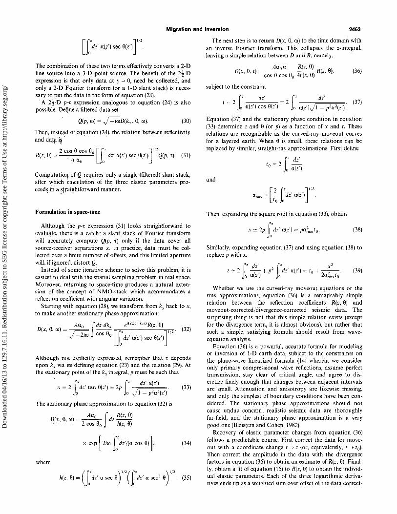
The combination of these two terms effectively converts a 2-D line source into a 3-D point source. The benefit of the 2i-D expression is that only data at y = 0, need be collected, and only a 2-D Fourier transform (or a I-D slant stack) is necessary to put the data in the form of equation (28).
A 2i-D p-'t expression analogous to equfltion (24) is also possible. De~ne a filtered data set
Q(p, (0) = J -iooD(kx , 0, (0). (30)
Then, instefld of equation (24), the relation between reflectivity and da~~t~ . .
R(z, 8) = . 0 dz' u(z') sec 8(z') Q(p, 't). (31) 2 cos 8 cos 8 [i' J1 12 u Uo 0
Computatio'l of Q requires only a single (filtered) slant stack, after which calculation of the three elastic parameters proceeds in a sffaightforward manner.
Formulation in space-time
Although the p-'t expression (31) looks straightforward to evaluate, there is a catch: a slant stack of Fourier transform will accurately compute Q(p, 't) only if the data cover all source-receiver separations x. In practice, data must be collected over a finite number of offsets, and this limited aperture will, if ignored, distort Q.
Instead of some iterative scheme to solve this problem, it is easiest to deal with the spatial sampling problem in real space. Moreover, returning to space-time produces a natural extension of the concept of NMO-stack which accommodates a reflection coefficient with angular variation.
Starting with equation (28), we transform from kx back to x, to make another stationary phase approximation:
_ Auo f dz dkx ei(20lT+kx x)R(z,8)
D(x, 0, (0) - ~ cos 8 [iZ J1 12' (32) v' - 210) 0 dz' u(z') sec 8(z')
o
Although not explicitly expressed, remember that 't depends upon kx via its defining equation (23) and the relation (29). At the stationary point of the kx integral, p must be such that
1z l' dz' u(z') x = 2 dz' tan 8(z') = 2p --r='=~c== o 0 Jl - p2U2(Z')
The stationary phase approximation to equation (32) is
Auo f R(z,8) P(x, 0, (0) = 2 cos 8
0 dz h(z, 8)
where
(33)
(34)
The next step is to return D(x, 0, (0) to the time domain with an inverse Fourier transform. This collapses the z-integral, leaving a simple relation between D and R, namely,
Auo u R(z, 0) ( 8) D(x, 0, t) = 8 8 4h( 0) R z" (36) cos cos 0 z,
subject to the constraint
t = 2 = 2 . (37) 1
z dz' 1Z dz'
o a(z') cos 8(z') 0 a(z')Jl - p2U2(Z')
Equation (37) and the stationary phase condition in equation (33) determine z and 8 (or p) as a function of x and t. These relations are recognizable as the curved-ray moveout curves for a layered earth. When 8 is small, these relations can be replaced by simpler, straight-ray approximations. First define
and
1z dz' t -2 -0- 0 u(z')
[2 rz J1 12
CXrms = ~ Jo dz' a(z')
Then, expanding the square root in equation (33), obtain
x ~ 2p r dz' u(z') = PU;ms to· (38)
Similarly, expanding equation (37) and using equation (38) to replace p with x,
t ~ 2 -, + pl dz' a(z') = to + -2--' 1z dz' 1Z x 2
o u(z) 0 2urms to (39)
Whether we use the curved-ray moveout equations or the rms approximations, equation (36) is a remarkflbly simple relation between the reflection coefficients R(z, El) and moveout-corrected/divergence-corrected seismic data. The surprising thing is not that this simple relation exists (except for the divergence term, it is almost obvious), but rather that such a simple, satisfying formula should result from waveequation analysis.
Equation (36) is a powerful, accurate formula for modeling or inversion of I-D earth data, subject to the constraints on the plane-wave linearized formula (14) wherein we consider only primary compressional wave reflections, assume perfect transmission, stay clear of critical angle, and agree to discretize finely enough that changes between adjacent intervals are small. Attenuation and anisotropy are likewise missing, and only the simplest of boundary conditions have been considered. The stationary phase approximations should not cause undue concern; realistic seismic data are thoroughly far-field, and the stationary phase approximation is a very good one (Bleistein and Cohen, 1982).
Recovery of elastic parameter changes from equation (36) follows il, predictable course. First correct the data for moveout with a coordinate change t-> z (or, equivalently, t-> to). Then correct the amplitude in the data with the divergence factors in equation (36) to obtain an estimate of R(z, 8). Finally, obtain a fit of equation (15) to R(z, 8) to obtain the individual elastic parameters. Each of the three logarithmic derivatives ends up as a weighted sum over offset of the data correct-
Dow
nloa
ded
04/1
6/13
to 1
29.7
.16.
11. R
edis
trib
utio
n su
bjec
t to
SEG
lice
nse
or c
opyr
ight
; see
Ter
ms
of U
se a
t http
://lib
rary
.seg
.org
/
2464 Stolt and Weglein
ed for moveout. The weight factors, which are different for each parameter so as to satisfy equation (15), represent the only substantial change from conventional moveout correction and stack.
REALISTIC LINEAR INVERSION GOALS
Because there normally are more than three offsets in the data, the relation in equation (15) provides more equations than unknowns. The inverse problem is therefore overdetermined; nevertheless, a good estimate of all three parameters is very difficult to obtain. A large range of angles is necessary to distinguish betweell the three parameters. This need is made clear if we express equation (15) in powers of pa = sin e:
1 [d In pa 2 2 (d In a ~2 d In p~2) R(z, e) ="2 -d-z - + P a -d-z - - 4 a 2 -d--:-'z'-'--
(40)
At normal incidence, only the first term (acoustic impedance) contributes. At 30 degrees, the coefficient of the last term is only 8 percent of that of the first term. The last term does not become as large as the first term until e = 52 degrees. This angle is not often achieved at depths of exploration interest, even if we could retain confidence in the linearized form at that angle.
The inverse to equation (40) will be, in most practical situations, ill-conditioned. The ability to extract reliably all three parameters from contemporary seismic data is likely to be more the exception than the rule. Even before noting that several factors external to a reflector can alter amplitudes as sin4 e, we realize we are in trouble. The three-parameter linearized inverse seems to be in a squeeze; to differentiate between the parameters, a large range of offset angles is required. On the other hand, if we look at angles which are too large, the linearized model may break down. In a practical situation, it may be possible to separate the three parameters only at moderate depths where the angular aperture is large.
A way to increase the reliability of an inverse to equation (40) is through use of a priori information to constrain the result. If we could reduce the effective number of parameters from three to two, we would be much better off. There are many ways to accomplish this reduction (each involving the risk of imposing a solution which may not be true), but all are beyond the scope of this paper. We do point out that neglecting changes in shear modulus is not the answer. Note from equation (40) that shear modulus plays an important role in the angular dependence of the compressional reflection coefficient and, indeed, may often dominate it. Only when confining attention to near-normal incidence can shear modulus be safely neglected.
Another pitfall comes from the limitations of the linearized approximation. Although this approximation may be "exact" in a continuous, smoothly variable medium, changes which are large over the sampling interval~and presumably rapid compared to the frequencies in the data~violate the validity conditions. Validity conditions are essentially that the fractional change in each elastic property must remain small even when multiplied by tan e. Weglein et al. (1985) pointed out that for a discrete change in one physical parameter, a Iin-
earized inversion formula always predicts changes in the other parameters also. These false predictions, or artifacts, also noted in Hanson (1984), can be significant.
These artifacts can, to some extent, be dealt with at a cost of slightly greater algorithmic complexity. The confidence in an inversion can be improved by using angles only within the confidence interval of the data. For example, assume that several incidence angles need to be specified to invert for elastic properties. The range of reasonable angles should be chosen consistent with the minimum and maximum offset of the experiment and the depth of the particular reflector. Postcritical data must also be avoided. Additionally, Weglein et al. (1985) presented a method for distinguishing artifacts from true parameter changes based on f-k filtering. In space-time, the simplest measure is to confine attention to incidence angles of less than about 45 degrees (Hanson, 1984). If all else fails, we can try to invert the full Zoeppritz reflection coefficient; however, not just relative but absolute sizes of parameters then come into play.
When talking of discretization problems, we acknowledge that not just the linearization approximation, but the whole physical model, can be placed in jeopardy. Changes which are too fast for the frequencies in the data to "see" directly can affect perceived physical properties in many ways, introducing time delays, attenuation, and anisotropy. In extreme cases, such effects can perturb or even invalidate inversion results.
If data quality does not justify multiparameter inversion, it still may be possible to solve for a single parameter. By confining attention to near-normal incidence, acoustic impedance becomes a legitimate target. Most useful would be the absolute value of this property, though that is an elusive target. Even with low-frequency information supplied (or inferred), integration of the logarithmic derivative is treacherous. Data noise and transmission effects accumulate and multiples in the data bias the result (a spurious spike in the reflectivity series, when integrated, alters the background level of the parameters). Data normalization remains a problem. We expect better results over short intervals. Under good conditions, it is possible to map the relative sizes of impedance changes accurately. Even for poor data, we expect to document the existence and possibly the sign of an impedance change (Weglein and Gray, 1983).
To summarize, multiparameter inversion methods are used to determine the configuration of physical properties. Depending upon the data, there are various levels at which data can be inverted. The first, least ambitious level is to determine, at a given subsurface location (in depth or time), whether some property (maybe acoustic impedance) has changed. At the next level, we also determine the sign or phase of this change. At a higher level, we acquire amplitude information. Slightly higher, we recognize the "signature" (e.g., an unmistakable increase in amplitude with offset, see Ostrander, 1984) of some target geologic entity. At a still higher level, we distinguish more than one physical property and determine the sign of each change. At the highest level, absolutely true values of all relevant physical properties are determined. Of course, the highest level is desired when we can get it. However, even if the highest level is unobtainable, useful information may still be available with the sign of a parameter change being easier to predict than its amplitude.
In practice, the power to resolve individual parameters must diminish with depth. At deeper levels, raypaths approach
Dow
nloa
ded
04/1
6/13
to 1
29.7
.16.
11. R
edis
trib
utio
n su
bjec
t to
SEG
lice
nse
or c
opyr
ight
; see
Ter
ms
of U
se a
t http
://lib
rary
.seg
.org
/
Migration and Inversion 2465
normal incidence, and only the ability to see acoustic impedance is left.
THE MULTIDIMENSIONAL INVERSE PROBLEM
The last decade has seen an explosion in migration and inversion technology. Since the early work of Claerbout demonstrated that wave-equation techniques were really applicable to seismic processing, a host of different processes have been presented. For a while, it seemed that competing technologies were developing-differential versus integral versus transform methods, then time migration verSus depth migration versus reverse time migration, and finally, migration versus inversion. The contemporary view is that all these approaches share a common theoretical base. The Earth being complex and variable, it is necessary and desirable to keep an arsenal of specialized tools which are similar, but each one is customized to a particular application.
The major difference between single-parameter waveequation inversion and wave-equation migration has turned out to be semantic; with its origins in scattering theory and applied mathematics, seismic inversion encourages a slightly different vocabulary than the more operationally based migration.
This is not to say that inversion concepts have not added to migration theory. Seismic inversion has provided a means to advance past recovery of reflectivity information to recovery of the physical changes which produce reflections. This, in turn, tied migration more firmly to I-D data processing concepts from which the relationship between reflectivity and Underlying physical changes has been better understood. inversion concepts also have provided a framework for dealing with experimental limitations in real data sets. For example, migration usually deals with the problem of a source wavelet by ignoring it. Set up as an inverse scattering problem, the effect of the source wavelet can be incorporated, and the changes to the wavelet through the various processing steps can be observed and calculated. Likewise, effects of finite source-receiver aperture can be built into the problem.
Evolution of migration and inversion
Seismic migration has been around a long time. Deterministic migration methods are probably as old as the earliest seismic data. The advent of digital computers encouraged the growth of statistical migration methods-in particular, the "arc swinging" algorithms, whose modern counterpart is Kirchhoff migration. The Claerbout concept of a moving coordinate system reduced the cost and increased the fidelity of seismic migration to the point where it could be considered part of a standard processing sequence. SooIi differential, integral, andf-k migration schemes abounded.
Cohen and Bleistein (1977) formulated the inverse seismic problem in terms of perturbation theory, presenting an apparent alternative to seismic migration. In this method, deviations from background values are solved by linearizing the inverse problem. The linearized inverse method developed by Bleistein and Cohen has concentrated on inversion of zero-offset seismic data by means of the scalar wave equation. This oneparameter inversion is now known to be closely related to poststack migration, both in theory and in practice. A oneparameter inversion is exactly right for zero-offset data. For
this case, there is enough iniormation to recover only one earth parameter. [Only one parameter contributes; equation (40) shows that only acoustic impedance contributes to normal incidence seismic data.]
For prestack inversion, the scalar wave equation does not suffice. Though the original work of Cohen and Bleistein discussed both scalar and elastic fields, seismic inversion methods were essentially scalar until Raz (1981a, b) introduced an inversion scheme for acoustic (variable velocity and density) data. A nice feature of Raz's I-D result (Raz, 1981a) was a space-time formula used to solve for density and velocity given data at two offsets. A second Raz result (Raz, 1981b) was a multidimensional linear solution for density and velocity perturbations. Clayton and Stolt (1981) also worked with the acoustic model, producing an f-k space result valid for variable background velocity and density. Raz (1982) published variable-velocity acoustic formulas which, with some restrictions, solve for absolute values of earth parameters. The importance of work with the acoustic wave equation should not be understated, particularly regarding advances in understanding of the multiparameter inverse problem. However, the acoustic wave equation does not quantitatively model reflections of compressional waves in the real Earth. As seen in equation (40), shear modulus changes make a major, perhaps dominant, contribution to the reflectivity away from normal incidence.
The elastic problem is more difficult to work with than the acoustic problem, mainly because it tends to lead toward lengthy equations. However, several researchers have described procedures, including Marfurt (1978), Clayton (1981), and recently Chen and Xie (1985) and Tarantola (1984).
The linear perturbation model
The first step in wrestling with the inverse seismic problem is to develop an adquate model of the reflection experiment and the reflection process. For a I-D earth, this is made simpler by a change of coordinates from depth to traveltime [equation (3)]. This change may not be possible or helpful when velocities vary laterally (Hagin and Gray, 1984). This does not mean that the multidimensional problem is intractable. A great many tools are still available. The linearized perturbation method is a simple, effective approach to the multidimensional problem. In this method, we begin with a known or predetermined background model, close enough to true Earth properties that we can consider them to be small deviations or perturbations of the model. Typically, the background model is expected to describe wave propagation in the earth with reasonable accuracy, neglecting the generation of reflected waves. The perturbations from the model then generate the reflection data.
To illustrate the concepts, we use the acoustic wave equation. Although admittedly inadequate, the acoustic wave equation leads to results which are simple to describe and, better yet, simple to generalize. For a point source at x" the total response P at x, including reflections, obeys the acoustic wave equation
[ V. _1_ V + 0)22 jP(X1Xs ; 0)) = -S(O))b(x - xs)' (41) p{x) p(x)a (x)
Dow
nloa
ded
04/1
6/13
to 1
29.7
.16.
11. R
edis
trib
utio
n su
bjec
t to
SEG
lice
nse
or c
opyr
ight
; see
Ter
ms
of U
se a
t http
://lib
rary
.seg
.org
/

2466 Stolt and Wegleln
The source term S(oo) represents the Fourier transform of a source wavelet.
The approximate (unperturbed) background wave field Go, due to an impulsive point source satisfies
( V. ~ V + 002 2)Go(XIXs; (0) = -8(x - xs)'
Po Pouo (42)
If Go is to track the propagation of a wave accurately, Uo should be close to the true velocity u. On the other hand, if Po and Uo vary too rapidly, Go will contain reflection energy. This may be all right, especially if we are using a successive approximation scheme. Ordinarily, it is desirable for Go to be reflection-free, if for no other reason than we are unlikely to know u and P sufficiently well a priori to reproduce accurately the reflections. The ideal choice for Uo and Po would be local averages of the true values, too slowly varying to produce significant reflection energy for frequencies where S(oo) is nonzero. Although we may fall short of this ideal in practice, we proceed on the assumption that Uo and Po are indeed local averages close to the true Earth parameters.
We designate the difference between the two wave operators in equations (41) and (42) as a potential V:
where
and
(1 1) 2 ( 1 1) V(x, (0) = V· -:- - - V + 00 -2 - --2 P Po pu Pouo
. a2 V 2( a1 ) =V·--+oo --2' P Pouo
Po a2 (x) = - - 1, P
Pou~ a1(x) = --2 - 1.
pu
(43)
This potential then contains the unknowns for which we would like to solve.
The difference D between the exact and modeled response obeys a simple identity
D(Xg I Xs; (0) = P(Xg I Xs; (0) - S(oo)Go(Xg I Xs; (0)
= f dx Go(xglx; oo)V(x, oo)P(xlxs; (0), (44)
which can be verified by applying the unperturbed wave operator to both sides of the equation. Equation (44) is nOhlinear in the potential because P (which depends upon the potential) appears inside the integral along with the potential. We linearize it simply by approximating P by SGo in the right-hand side of equation (44):
D(xglxs; oo)~S(oo) f dx Go(xglx; oo)V(x, oo)Go(xlxs; (0). (45)
If Go is a good model of the transmitted wave minus reflections, then the interpretation of equation (45) is clear: The response P at Xg due to a source at Xs is the sum of a direct arrival SGo and an integral over all possible reflection points. The integrand is the product of a transmitted wave from Xs to the reflection point x, times a reflection term V(x, (0), times a transmitted wave from x to xg • Should Go include reflection energy, then the equation still holds, but the interpretation does not. We state that the difference between the actual data
and the modeled data should approximately obey the linearized integral equation (45).
The form of equation (45) is reminiscent of the I-D equation (14). However, there are two differences. The first is that the transmission term in equation (14) incorporates the correct velocity, whereas Go is guided by an approximation uo. The second is that V(x, 00), though clearly related to reflectivity, is not exactly a reflection coefficient. The first difference is both good and bad. The good part is that it allows Go to be constructed without an exact knowledge of density and velocity. (If we had that knowledge, the inverse problem ~ould be solved already.) The bad part is that, to the extent that Uo differs from u, reflection points will be mislocated upon inversion. [This is also true for the I-D case. The reflection coefficient R(1:, p) can be solved using equation (22) from the reflection data, even if velocity as a function of depth is unknown. Conversion from traveltime to correct depth, however, is possible. only with the correct velocity.] A discussion of the second difference, the relation between V and R, follows.
WKBJ approximation in three dimensions
Some of the complexity of equation (45) can be removed by invoking the WKBJ approximation. Suppose that Go closely approximates a delta function wavefront so that in the frequency domain,
Go (Xg I Xs; 00) ~ go (Xg I x.) exp [joo1:(Xg I xs)]. (46)
Here, go is the amplitude of the wavefront, which is assumed to be slowly varying and 1: is the traveltime from source to receiver, which varies rapidly. Indeed,
(47)
while the direction of V1: defines the local direction of the raypath from source to receiver. The amplitude go is determinable from the first transport equation (Morse and Feshbach, 1953) for the WKBJ expansion.
Using the WKBJ approximation for Go, equation (45) reduces to
D(xglxs; (0) = 002S(00) fdX go(Xglx)g~(XIX') v(x, 8) PoUo
x exp {ioo[1:(xg I x) + 't(x I xs)]}' (48)
where v(x, 8) is a simplified potential function denuded of frequency arid differential operator dependence:
V(X, 8) = (P;u~6 - 1) + cos (28) (ppo - 1). (49)
The angle 28 is the angle between incident and reflected rays at the reflection point x. Although not explicit in this formula, u depends upon source and receiver coordinates Xs and Xg
through the angle of incidence 8. The simplification in equation (49) of the potential function is made possible by the WKBJ approximation, which is essentially the geometrical acoustics approximation. The impulse response Go has a welldefined direction at every point, so the derivatives contained in V are easily evaluated. The potential v(x, 8) is seen to be the sum of two terms, one involvmg density ~p/p and the other bulk modulus ~(pU2)/pU2. As such, it is hardly identical to the I-D reflection coefficient equation (15). However, if Po ~ P and Uo ~ u, then
Dow
nloa
ded
04/1
6/13
to 1
29.7
.16.
11. R
edis
trib
utio
n su
bjec
t to
SEG
lice
nse
or c
opyr
ight
; see
Ter
ms
of U
se a
t http
://lib
rary
.seg
.org
/

Migration and Inversion 2467
poa~ Po v(x, 9) ~ In --2 + cos (29) In -,
pa p (50)
and better yet, 1
- - sec2 9 - v(x) ~ - -- + sec2 9 --1 0 1 [0 In p 0 In a] 4 OZ 2 OZ OZ
== R(x, 9). (51)
The right-hand side of equation (51) is recognizable as the first two terms of the reflection coefficient equation (15). We therefore identify R(x, 9) as a reflection coefficient2 and v(x, 9) as an integrated angle-filtered reflection coefficient. The last term in (15) does not appear in (51) because shear modulus changes are invisible to the acoustic wave equation. A way to view the shear modulus term is as a mysterious leakage of energy to and from an unseen other mode of propagation. As such, we are free to add it to equation (51). This step can be justified by recourse to the elastic wave equation (Clayton, 1981).
2!-D formulation
If v(x, 9) does not change significantly in the y direction, equation (48) for D can be further simplified. We confine data values to Yg = Ys = O.
The only significant Y dependence in the right-hand side of equation (48) is in the traveltimes t(xg I x) and t(x I xs). These are clearly minimized at Y = O. The go terms can be replaced by their values at Y = 0, leaving
D(xglxs; (0) = oo 2S(oo) f dx
f v(x, z, 9) x dz go (Xg I x, z)go (x, z I xs) 2
poao
x f dy exp [ioo('t(xg I x) + 't(x I xs)]. (52)
Writing traveltime in the vicinity of y = 0 as
(53)
the y integral in equation (52) can be evaluated by stationary phase, leaving
oo2
S(oo) f f D(xglxs; (0) = fo dx dz
'To proceed to equation (51) from equation (50), we assumed that ao and Po are slowly varying, i.e., have negligible derivatives and do not produce noticeable reflections. The term cos (29) which depends on the background velocity is likewise assumed to have negligible zderivative. For background velocities which do produce reflections, equation (51) becomes the difference between modeled and actual reflection coefficients. For a slowly varying background, we emphasize what may be obvious: Although the potential technically depends on the choice of background parameters, it is actually, extremely insensitive to them. The logarithmic approximation in equation (51) is really an improvement to the form of equation (49), as noted in the section on I-D. 2Strictly, the quantity R defined in equation (51) is a true reflection coefficient only when local velocity structure ao does not vary laterally. In general, the true reflection coefficient would be a derivative taken normal to local structure. Here we chose, somewhat arbitrarily, to work with the quantity R as defined in equation (51) and to call R, somewhat disingenuously, a reflection coefficient.
(54)
Equation (54) differs little from a true 2-D formula. We observe the 45 ~ree phase term fo and a divergence correction term yI'tyy , which together convert a 3-D experiment along the line y = 0 into an equivalent 2-D form. Provided tyy
can be estimated (which, in the worst case, can be accomplished by ray shooting), the 2!--D form presents little additional complication. Bleistein (1985) presented a formula for calculating 'tyy from in-plane raypath information. The result is 'tyy = 2/cr, where cr is a ray parameter related to arc length s on the ray by dcr/ds = a(x, z).
Multidimensional linearized inversion
A prescription for inversion of the multidimensional formula in equation (48) or (54) is given in Clayton and Stolt (1981). The prescription involves a form of migration. We first downward-continue to depth z the reflection data D, both source and receiver coordinates. This, in principle, is done by application of the divergence theorem to both source and receiver coordinates along the surface z = O. The amplitude of the downward continuation must be carefully computed and adjusted for divergence effects. The zero-time component of the downward-continued data is extracted by summing over frequencies, effecting a migration of the data. By retaining migrated data for Xg of. xs ' information regarding angles of incidence is also retained. 3 To decode the angle of incidence information, we Fourier-transform the migrated data over all spatial coordinates. The result is proportional to the Fourier transform of the reflection coefficient in equation (51).
For the special case of a depth-dependent background velocity, we write an explicit 2!--D formula (see the Appendix)
R(kg - ks' kz' 9)
= ~ sec2 9 f dz eik,z 4i
x f ~oo q(z) ((ZdZ' aoq)112 fo poao Jo qgqs
[q (O)q (0)J I
12
[ iZ J x 9 s exp - ioo dz' q/a D(kg I ks ; (0). qg (z)qs (z) 0
(55)
In this expression,
(56)
3For data at Xg i' x, to be nonzero as t---> 0 may appear to violate causality. In fact, it is true that the data must go to zero (within the limits of source-receiver size and bandwidth) as Xg moves away from x,. There is still the question, however, of how the data approach zero, and it turns out (because of the angular dependence of reflectivity) the limit is sensitive to the direction of approach to a reflection point. The migrated data are not a simple delta function of Xg - x" though they are sharply peaked. A Fourier transform over offset and depth reveals that the migrated data are not constant in offset wavenumber (which would correspond to a delta function in offset) but, rather, they form a slowly varying function of offset wavenumber divided by depth wavenumber, [see equation (59)] i.e., a slowly varying function of angle of incidence.
Dow
nloa
ded
04/1
6/13
to 1
29.7
.16.
11. R
edis
trib
utio
n su
bjec
t to
SEG
lice
nse
or c
opyr
ight
; see
Ter
ms
of U
se a
t http
://lib
rary
.seg
.org
/

2468 Stolt and Weglein
(57)
and
q(z) = qg (z) + q. (z). (58)
R(km' kz' 9) is the double Fourier transform of the reflection coefficient R(x, z, 9) at the angle of incidence 9. 9 is determined in this formula as the ratio of offset spatial frequency to depth spatial frequency:
tan 9 = (kg + k.)/kz • (59)
Equation (55) is an extension [provided we use equation (15) for R] of the I-D inversion formulas developed in the previous section. The prescription is to (1) Fourier transform the data from xg, x., and t to kg, k., and 00; (2) downward continue to depth z with a phase shift and the amplitude correction given inside the 00 integral of equation (55); (3) sum over 00 to effect a migration; (4) when the migration is complete for all z, Fourier transform from z to kz to obtain the perturbation; (5) multiply by kz sec2 9/4i to convert the perturbation to a reflection coefficient; and (6) inverse Fourier transform over k = k - k. and kz to yield a spatial map of the local reflectivit; as :
function of incidence angle. Although explicit, equation (55) does look unwieldy. Given
some further approximations (e.g., straight raypaths), some of the complexity can be removed. For example, if background velocity is assumed constant, then both the 00 and z integrals are trivially evaluated, leaving
,--~-------------R(k _ k k 9) = ~ J4ikz qg q.[1 + (kg + k.)2/k;
9 ., Z' Po 1+(kg -k.)2/k;
D(kg I k.; (0),
where R is a divergence-adjusted version of R:
R(x, z, 9) = R(x, z, 9)!Jz,
and 00 and kz are related as
00 J~J~ ~=-~+~= ~-~+ ~-~. Uo Uo Uo
(60)
(61)
(62)
We showed above that the extension of the NMO-stack concept to accommodate an angular dependent reflection coefficient allowed the inversion for the three elastic parameters in a vertically varying medium. The elastic inversion then requires three different weighted sums over offset of moveout and divergence-corrected data. The analogous multidimensional situation results in different specific weighted averages of D(kg, k., (0) (or its downward continued generalization) providing either a migration or the acoustic or elastic components of reflectivity. If the background is constant (and we assume line sources) the elastic generalization of the Clayton and Stolt (1981) result leads to (see, e.g., Clayton, 1981),
3
D(kg, k., (0) = I Aj(kg, k., oo)aj(kg - k., kz), (63) i=l
where
A3 = - ~ (- 2~~ [k q + k q ]2) 4q. qg 002 g. • 9 ,
and the aj are the Fourier transforms of
Pou~ a1 =---1
pu2 '
Po a2 = --1, P
a3
= Po ~~ - 1 p~2 .
The coefficients Al and A2 are identical to those in Clayton and Stolt (1981). They appear slightly different because q and q. are defined slightly differently there. The coefficien: A , describing leakage of compressional energy into a shear mod~, does not appear in Clayton and Stolt. From equation (63) the a j are reconstructed [see e.g. Clayton and Stolt (1981)] as weighted averages of D(kg, k., (0). Equation (63) can be rewritten as
D(kg, k., (0) = 4 Po (a1 + cos 29a2 - 2~~ sin2 29a3), qgq. Uo
where 9 is the half angle between the incident and reflected pressure wave
9 = i[sin- 1 (kguo/OO) + sin- 1 (k.uo/OO)].
The elastic generalization of equation (49) is
2~2 v(x, 9) = a1(x) + cos 29a2 (x) - u~o sin2 29a3 (x),
and using equation (15) the relationship between the elastic ~x, 9) and R(x, 9) is also given by equation (51). Equation (63) l~ almost ~he same as equation (60). They differ because equation (60) Incorporates the 21-D correction [equation (A-9) of Clayton and Stolt (1981)].
For the more general case, Cohen and Hagin (1985) promised to generalize the zero-offset, space-time inversion formula to pres tack data.
Whichever form we choose for a migration and inversion operator, a few conclusions can be made.
1. Inverting for the elastic parameters does not greatly complicate the migration process. We expect the expense of a migration and inversion algorithm to be dominated by the migration process.
2. The limitations in resolving all the elastic parameters noted for I-D inversion still exist. The fk formulas in equations (55) and (60) obscure the effects of finite source-receiver aperture but do not eliminate them. In fact, the resolving power of migration and inversion must diminish with depth, leaving ultimately only migration.
NONLINEAR METHODS
There are a small number of exact, nonlinear, multidimensional methods for solving acoustic and elastic inverse problems. For excellent reviews of I-D methods, see Newton (1966) or Burridge (1980). For the multidimensional problem, there are several approaches which have been taken. One is to
Dow
nloa
ded
04/1
6/13
to 1
29.7
.16.
11. R
edis
trib
utio
n su
bjec
t to
SEG
lice
nse
or c
opyr
ight
; see
Ter
ms
of U
se a
t http
://lib
rary
.seg
.org
/

Migration and Inversion
invert the Born series iteratively. This line of research was CONCLUSION
2469
originated by Jost and Kohn (1951), Kay and Moses (1955), Prosser (1969), and Razavy (1975), and was introduced to geophysics by Weglein et al. (1981) and Stolt and Jacobs (1980). The convergence properties of this series solution were studied by Prosser. Only "small" reflection data would allow the series to converge. Weglein (1982b) generalized some earlier Razavy (1975) work to invert a "distorted" Born series for an arbitrary background, thus allowing reflections and multiples in the background model. The goal was to allow accommodation of" larger" reflection data.
Another approach to solving the multidimensional inverse problem derives from the Gelfand-Levitan/Marchenko integral equation methods originally designed for the Schrodinger equation (Agronovich and Marchenko, 1963; Faddeev, 1963). In one dimension, a Liouville transformation exists to map elastic and acoustic problems to a Schrodinger equation and hence allows the machinery designed for the latter to be used. An interesting paper by Berryman and Greene (1980) showed that a discretized form of these integral equation methods leads to the original Goupillaud (1961) equal-traveltime inverse solution. However, even though multidimensional Schrodinger equations had been inverted (in theory) in two and three dimensions in Newton (1981) and Cheney (1984), no corresponding Liouville transformation was found to allow a multidimensional acoustic or elastic equation to be mapped into a multidimensional Schrodinger equation. Recently, Coen et al. (1984) presented a method for inverting a 2-D, variable-density acoustic equation by collecting point source data. Transforming the data over the dimension of which the medium is independent allows a 2-D Schrodinger equation to evolve. The Cheney 2-D Marchenko equation is used to solve the problem. Transmission as well as reflection data would be required.
Several authors have recently approached the multidimensional linear and nonlinear inverse problem from the generalized linear inverse point of view. Among these are Chen and Xie (1985), Berkhout (1984), Keys and Weglein (1983), and Tarantola (1984). The method basically consists of approaching the Fredholm I integral equations, which result from the linear Lippmann-Schwinger equation, by a generalized linear inverse method. These methods impose the constraints to determine a model which (1) is close to the reference model and (2) has the predicted data residuals close to the actual residuals. The residuals are the difference between the data and the background model-generated data. This method determines a "solution" whether or not the original integral equation possessed a single solution, many solutions, or no solutions. Confidence in these methods was discussed by several authors---e.g., Treitel and Lines (1985). The question of the convergence of the iterative solution (and the convergence to the "answer") of the generalized linear inverse approach to the nonlinear problem has yet to be addressed adequately.
Common to all the nonlinear approaches is a demand for massive amounts of computer power. Given the size of the seismic problem (a good-size 3-D survey should be looking at 108 to 109 subsurface points) and the fact that any nonlinear method must employ point-to-point correlations over substantial distances (roughly squaring the size of the problem), we begin to realize that today's "supercomputers" represent but a small step in the right direction toward the facilities necessary for a complete solution to the seismic problem.
Seismic processing has made significant advances during the last decade. Imaging techniques have matured and merged with seismic inversion to form potentially powerful tools for unraveling geologic structure and lithology under ideal conditions. A general principle for inversion is that the more ambitious the goal, the more hazardous and sensitive the procedure. However, the potential exists for predicting the three elastic parameters from compressional data. Practical difficulties are many. They include limitations in data quality (some removable with extra effort and some not) and in available computer resources.
ACKNOWLEDGMENTS
We thank the management of Co no co Inc. and Sohio Petroleum Company for permission to publish this paper. Roger Parsons helped develop some of the material and made several helpful comments besides. Doug Hanson and Bob Keys also provided good advice and commentary. Professor Norman Bleistein of the Colorado School of Mines reviewed the paper and made 15 suggestions; all of his comments were good and have been responded to. We are most grateful to him. Finally, we thank Donna Stolt and Christine Weglein for their support and patience while this paper was being written.
REFERENCES
Aki, K., and Richards, P., 1979, Quantitative seismology-theory and methods: W. H. Freeman and Company.
Agronovich, Z. S., and Marchenko, V. A., 1963, The inverse problem of scattering theory: Gordon and Breach.
Berkhout, A. J., 1984, Multidimensional linearized inversion and seismic migration: Geophysics, 49,1881-1895.
Berryman, 1. G., and Greene, R. R., 1980, Discrete inverse methods for elastic waves in layered media: Geophysics, 45, 213-233.
Bleistein, N., 1985, Two-and-one-half dimensional in-plane wave propagation: Geophys. Prosp., to appear.
Bleistein, N., and Cohen, J. K., 1979, Velocity inversion for acoustic waves: Geophysics, 44,1077-1087. ~- 1982, Velocity inversion-Present status, new directions: Geo
physics, 47, 1497-1511. Bleistein, N., and Handelsman, R., 1975, Asymptotic expansions of
integrals: Holt, Rinehart and Winston. Burridge, R., 1980, The Gelfand-Levitan, the M~rchenko and the
Gopinath-Sondhi integral equations of inverse scattering theory, regarded in the context of inverse impUlse-response problems: Wave Motion, 2, 305-323.
Chen, Y. M., and Xie, G. Q., 1986, Simultaneous determination of bulk modulus, shear modulus, and density variations from seismic data: Geophysics, 51.
Cheney, M., 1984, Inverse scattering in dimension II: 1. Math. Phys., 25,94.
Cheng, G., and Coen, S., 1984, The relationship between Born inversion and migration for common midpoint stacked data: Geophysics, 49, 2117-2131.
Clayton, R. W., 1981, Wavefield inversion methods for refraction and reflection data: Stanford Explor. Proiect Rep. No. 27 Stanford CA. J"
Clayton, R. W., and Stolt, R. H., 1981, A Born-WKBJ inversion method for acoustic reflection data: Geophysics, 46, 1559-1567.
Coen, S., 1981, Density and compressibility profiles of a layered acoustic medium from precritical incidence data: Geophysics 46 1244-1246. ' ,
-- 1982, Velocity and density profiles of a layered acoustic medium from common source-point data: Geophysics, 47, 898-905.
Coen, S., Cheney, M., and Weglein, A., 1984, Velocity and density of a two-dimensional acoustic medium from point source surface data: J. Math. Phys., 25,1857-1861.
Cohen, J. K., and Bleistein, N., 1977, An inverse method for determining small variations in propagation speed: Soc. Ind. Appl. Math., J.
Dow
nloa
ded
04/1
6/13
to 1
29.7
.16.
11. R
edis
trib
utio
n su
bjec
t to
SEG
lice
nse
or c
opyr
ight
; see
Ter
ms
of U
se a
t http
://lib
rary
.seg
.org
/

2470 Stolt and Wegleln
Appl. Math., 32,784-799. Faddeev, L. D., 1963, The inverse problem in the quantum theory of
scattering: J. Math. Phys., 4, 72-104. . Goupillaud, P. L., 1961, An approach to inverse filtering of near
surface layer effects from seismic records: Geophysics, 26, 754-760. Hagin, F. G., and Gray, S. H., 1984, Traveltime (like) variables and
the solution of velocity inverse problems: Geophysics, 49, 758-766. Hanson, D. W., 1984, Multiparameter seismic inversion using the
Born approximation: Ph.D. thesis, Univ. of Wyoming. Hooshyar, M. A., and Razavy, M., 1983, A method for constructing
wave velocity and density profiles from the angular dependence of the reflection coefficient: J. Acoust. Soc. Am., 73, 19-23.
Howard, M. S., 1983, Inverse scattering for a layered acoustic medium using the first-order equations of motion: Geophysics, 48, 163-170.
Jacobs, B., and Stolt, R. H., 1980, Seismic inversion in a layered medium-the Gelfand-Levitan algorithm: Stanford Explor. Project Rep. No. 24,109-134.
Jost, R., and Kohn, W., 1951, Construction of a potential from a phase shift: Phys. Rev., 102, 559-567.
Kay, I., and Moses, H. E., 1955, The determination of the scattering potential from the spectral measure function: Nuovo Cimento II, 917.
Keys, R. G., and Weglein, A. B., 1983, Generalized linear inversion and the first Born theory for acoustic media: J. Math. Phys., 24, 1444-1449.
Lindseth, R. 0., 1979, Synthetic sonic logs-a process for stratigraphic interpretation: Geophysics, 44, 3-26.
Marfurt, K. J., 1978, Elastic wave equation migration-inversion: Ph.D. thesis, Columbia Univ.
McAulay, A. D., 1985, Prestack inversion with plane-layer pointsource modeling: Geophysics, SO, 77-89.
Morse, P. M., and Feshbach, H., 1953, Methods of theoretical physics, Parts I and II: McGraw-Hili Book Co.
Newton, R. G., 1966, Scattering theory of waves and particles: McGraw-Hili Book Co.
--- 1981, Inversion of reflection data for layered media: A review of exact methods: Geophys. J. Roy. Astr. Soc., 65,191-215.
Ostrander, W. 1., 1984, Plane-wave reflection coefficients for gas sands at nonnormal angles of incidence: Geophysics, 49,1637-1648.
Phinney, R. A., and Frazer, L. N., 1978, On the theory of imaging by Fourier transform: Presented at the 48th Ann. Internat. Mtg. and Expos., Soc. Explor. Geophys., San Francisco.
Prosser, R. T., 1969, Formal solutions of inverse scattering problems: J. Math. Phys., 10, 1819-1822.
Raz, S., 1981a, Three-dimensional velocity profile inversion from finite offset scattering data: Geophysics, 46, 837-842. .
--- 1981b, Direct reconstruction of velocity and density profiles from scattered wave data: Geophysics, 46,832-836.
--- 1982, A procedure for multidimensional inversion of seismic data: Geophysics, 47, 1422-1430.
Razavy, M., 1975, Determination of the wave velocity in an inhomogeneous medium from the reflection coefficient: J. Acoust. Soc. Am., 58,956-963.
Stolt, R. H., and Benson, A. K., 1985, Seismic migration: Geophysical Press.
Stolt, R. H., and Jacobs, B., 1980, Inversion of seismic data in a laterally heterogeneous medium: Stanford Explor. Project Rep. No. 24, 135-152.
Tarantola, A., 1984, Inversion of seismic reflection data in the acoustic approximation: Geophysics, 49,1259-1266.
Treitel, S., Gutowski, P. R., and Wagner, D. E., 1982, Plane-wave decomposition of seismograms: Geophysics, 47,1375-1401.
TreiteI, S., and Lines, L., 1985, Inversion with a grain of salt: Geophysics, SO, 99-109.
Ware, J. A., and Aki, K., 1969, Continuous and discrete inversescattering problems in a stratified elastic medium, 1: Plane waves at normal incidence: J. Acoust. Soc. Am., 45, 911-921.
Weglein, A. B., 1982a, Multidimensional seismic analysis: Migration and inversion: Geoexplor., 20, 47-60.
--- 1982b, Near field inverse scattering formalism for the three dimensional wave equation: The inclusion of a priori velocity information: J. Acoust. Soc. Am., 71, 1179-1182.
Weglein, A. B., Boyse, W. E., and Anderson, 1. E., 1981, Obtaining three-dimensional velocity information directly from reflection seismic data: An inverse scattering formalism: Geophysics, 46, 1116-1120.
Weglein, A. B., and Gray, S. H., 1983, The sensitivity of Born inversion to the choice of reference velocity-a simple example: Geophysics, 48, 36-38.
Weglein, A. B., Violette, P. B., and Keho, T. H., 1986, Using a constant background multiparameter Born theory to obtain exact inversion goals: Geophysics, 51.
Weglein, A. B., and Wolf, M. A., 1986, Prestack migration and Born inversion: Presented at the 55th Ann. Internat. Mtg. and Expos., Soc. Explor. Geophys., Washington, D. C.
REFERENCES FOR GENERAL READING
Aminzadeh, F., and Mendel, 1. M., 1983, Normal incidence layered system state-space models which include absorption effects: Geophysics, 48, 259-271.
Bamberger, A., Chavent, G., Hernon, c., and Lailly, P., 1982, Inversion of normal incidence seismograms: Geophysics, 47, 757-770.
Baysal, E., Kosloff, P. D., and Sherwood, 1. W. C., 1984, A two-way nonreflecting wave equation: Geophysics, 49,132-141.
Berkhout, A. J., 1980, Seismic migration-imaging of acoustic energy by wave field extrapolation: Elsevier, North Holland Publishing Company.
--- 1983, High resolution techniques: new developments in seismic exploration: Preprint from the Eleventh World Petroleum Congress, Panel Discussion 4.
Berteussen, K. A., and Ursin, B., 1983, Approximate computation of the acoustic impedance from seismic data: Geophysics, 48, 1351-1358.
Bleistein, N., Cohen, J. K., and Hagin, F. G., 1985, Computational and asymptotic aspects of velocity inversion: Geophysics, 50.
Carrion, P. M., and Kuo, J. T., A method for computation of velocity profiles by inversion of large offset records: Geophysics, 49, 1249-1258.
Carrion, P. M., and Foster, D., 1985, Inversion of band-limited seismic data in the presence of multiples and low velocity zones: Geophysics, SO, 759-765.
Carter, J. A., and Frazer, L. N., 1985, Accommodating lateral velocity changes in Kirchhoff migration by means of Fermat's principle: Geophysics, 49, 46-53.
Case, K. M., and Chiu, S. c., 1973, The discrete version of the Marchenko equations in the inverse scattering problem: J. Math. Phys., 14, 1643-1647.
Case, K. M., and Kac, M., 1973, A discrete version of the inverse scattering problem: 1. Math. Phys., 14, 594-603.
Castle, R. J., 1978, Wave-equation migration in the presence of lateral velocity variations: Geophysics, 47, 1001-1011.
Chun, J. H., and Jacewitz, C. A., 1981, Fundamentals of frequency domain migration: Geophysics, 46,717-733.
Claerbout,1. F., 1968, Synthesis of a ILyered medium from its acoustic transmission response: Geophysics, 33, 264-269.
--- 1970, Coarse grid calculations of waves in inhomogeneous media with application to delineation of complicated seismic structure: Geophysics, 35, 407-418.
--- 1971, Toward a unified theory ofreflector mapping: Geophysics, 36, 467-481.
1976, Fundamentals of geophysical data processing: McGraw-Hili Book Co.
Claerbout, J. F., and Doherty, S. M., 1972, Downward continuation of moveout corrected seismograms: Geophysics, 37, 741-768.
Cohen, J. K., and Hagin, F. G., 1985. Velocity inversion using a stratified reference: Geophysics, SO, 1689-1700.
Cooke, D. A., and Schneider, W. A., 1983, Generalized linear inversion of reflection seismic data: Geophysics, 48, 665-676.
Cressman, K. S., 1968, How velocity layering and steep dip affect COP: Geophysics, 33,399.
Diebold, J. B., and Stoffa, P. L., 1981, The traveltime equation, tau-p mapping, and inversion of common-midpoint data: Geophysics, 46, 238-254.
Dix, C. H., 1955, Seismic velocities from surface measurements: Geophysics, 20, 68-86.
Dubrulle, 1983, Numerical methods for the migration of constant offset sections in homogeneous and horizontally layered media: Geophysics, 48, 1195-1203.
Esmersoy, G., Oristaglio, M., and Levy, B., 1985, Multidimensional Born velocity inversion: Single wide band point source: J. Acoust. Soc. Am., submitted November 1984.
Gazdag, J., 1978, Wave equation migration with the phase-shift method: Geophysics, 43,1342-1351.
Gazdag, J., and Sguazzero, P., 1984, Migration of seismic data by phase shift plus interpolation: Geophysics, 49,124-131.
Gjl2lystdal, H., and Ursin, B., 1981, Inversion of reflection times in three dimensions: Geophysics, 46, 972-983.
Gray, S. H., 1984, The relationship between "direct, discrete," and "iterative, continuous" one-dimensional inverse methods: Geophysics, 49, 54-59.
Hagin, F. G., and Cohen, J. K., 1984, Refinements to the linear velocity inversion theory: Geophysics, 49,112-118.
Hatton, L., Lamer, K. L., and Gibson, B. S., 1981, Migration of seismic data from inhomogeneous media: Geophysics, 46, 751-767.
Hron, M., and Razavy, M., 1977, Two discrete forms of the inverse scattering problem: Can. 1. Phys.,55, 1434-1441.
Hubral, P., 1983, Computing true amplitude reflections in a laterally inhomogeneous earth: Geophysics, 48,1051-1062.
Dow
nloa
ded
04/1
6/13
to 1
29.7
.16.
11. R
edis
trib
utio
n su
bjec
t to
SEG
lice
nse
or c
opyr
ight
; see
Ter
ms
of U
se a
t http
://lib
rary
.seg
.org
/

Migration and Inversion 2471
--- 1977, Time migration-some ray theoretical aspects: Geophys. Prosp., 25, 738-745.
Jacobs, A., 1982, The prestack migration of profiles: Stanford Explor. Project Rep. No. 34, Stanford, CA.
Jain, S., and Wren, A. E., 1980, Migration before stack-procedure and significance: Geophysics, 45, 204-212.
Jaulent, M., 1976, Inverse scattering problems in absorbing media: 1. Math. Phys., 17, 1351-1360.
Kjartansson,E., 1979, Attenuation of seismic waves in rocks: Stanford Explor. Project Rep. No. 23, Stanford, CA.
Kosloff, D. D., and Baysal, E., 1983, Migration with the full acoustic wave equation: Geophysics, 48, 677-687.
Krueger, R. 1., 1978, An inverse problem for an absorbing medium with multiple discontinuities: Quant. Appl. Math., 36, 235-253.
Kuo, J. T., and Dai, T. F., 1984, Kirchhoff elastic wave migration for the case of noncoincident source and receiver: Geophysics, 49, 1223-1238.
Lamer, K. L., Hatton, L., and Gibson, B. S., 1981, Migration of seismic data from inhomogeneous media: Geophysics, 46,751-767.
Lewis, S. A., 1984, Principle of reverse-time migration: Geophysics, 49,581-583.
Levinson, N., 1949, The Wiener RMS error criterion in filter design and prediction, Appendix B, in Extrapolation, interpolation, and smoothing of stationary time series with engineering applications: Wiener, N., Ed., John Wiley and Sons, Inc., 129-148.
Lindsey, J. P., 1984, Seismic determination of reservoir stratigraphy and parameters: Presented at seismic stratigraphy seminar in Oklahoma City, February, Geoquest International, Inc.
Lui, C Y., 1984, Born inversion applied to reflection seismology: Ph.D. thesis, Tulsa Univ.
May, B. T., and Covey, J. D., 1981, An inverse method for computing geologic structures from seismic reflections-Zero-offset case: Geophysics, 46, 268-287.
Mendel, 1. M., Kormylo, J., Aminzadeh, F., Lee, J. S., and HabibiAshrari, P., 1981, A novel approach to seismic signal processing and modeling: Geophysics, 46, 1398-1414. .
Neidell, N. S., and Poggiagliolmi, E., 1977, Stratigraphic modeling and interpretation-geophysical principles and techniques, in Payton, C E., Ed., Seismic stratigraphy-application to hydrocarbon exploration: Am. Assn. Petr. Geol. Memoir 26, 389-416.
O'Doherty, R. F., and Anstey, N. A., 1971, Reflections on amplitudes: Geophys. Prosp., 19, 430-458.
Oldenburg, D. W., Scheuer, t., and Levy, S., 1983, Recovery of the acoustic impedance from reflection seismograms: Geophysics, 48, 1318-1337.
Oldenburg, D. W., Levy, S., and Stinson, K., 1984, Root mean square velocities and recovery of the acoustic impedance: Geophysics, 49, 1653-1663.
Ramm, A. G., and Weglein, A. B., 1984, Inverse scattering for geophysical problems. II. Inversion of acoustical data: 1. Math. Phys., 25,3231-3234.
Raz, S., 1981, An explicit profile inversion: Beyond the Born model: Radio Science, 16, 347-355.
Schneider, W. A., 1978, Integral formulation for migration in two and three dimensions: Geophysics, 43, 49-76.
Schultz, P. S., and Sherwood, 1. W. C, 1980, Depth migration before stack: Geophysics, 45,376-393.
Sheriff, R. E., 1971, Limitations on resolution of seismic reflections and geolgoic detail derivable from them, in Payton, C E., Ed., Seismic stratigraphy-applications of exploration: Am. Assn. Petro Geol. Memoir 26, 3-14.
Snyder, A, 1979, Common shot gather modeling and inversion: Stanford Explor. Project Rep. No. 16, Stanford, CA, 59-81.
Stolt, R. H., 1978, Migration by Fourier transform: Geophysics, 43, 23-48.
Taylor, 1. R., 1972, Scattering theory: John Wiley and Sons, Inc. Temme, P., 1984, A comparison of common-midpoint, single-shot,
ahd plane-wave depth migration: Geophysics, 49,1896-1907. Thorson, 1., 1980, Synthetic examples of prestack migration: Stanford
Explor. Project Rep. No. 24, 5-32. Treitel, S., and Lines, L. R., 1982, Linear inverse theory and deconvo
lution: Geophysics, 47,1153-1159. Ursin, B., 1981, Error estimates for inverse modeling schemes using
seismic traveltimes: Geophysics, 46,1227-1234. Weglein, A. B., 1985, The inverse scattering concept and its seismic
application, in Fitch, A. A., Ed., Developments in geophysical methods, 6: Elsevier Science Publishers.
Weston, V. H., and Krueger, R. 1., 1973, On the inverse problem for a hyperbolic dispersive partial differential equation II: 1. Math. Phys., 14,406-408.
Wiggins, J. W., 1984, Kirchhoff integral extrapolation and migration of nonplanar data: Geophysics, 49, 1239-1248.
Yilmaz, 0., and Chambers, R. E., 1984, Migration velocity analysis by wave field extrapolation: Geophysics, 49,1664-1674.
APPENDIX
DERIVATION OF THE INVERSE FORMULA FOR A STRATIFIED BACKGROUND
There are a few steps between the general 2t-D modeling formula in equation (54) and the stratified inverse in equatiort (55). The first step is to write a formula for the stratified 2-D Green's function Go. From Clayton and Stolt (1981)
Go (x, zlx', z'; w)
= -=-!. f dk eik,(x-x') [po (z)Po (z')uo (z)uo (Z')J I/2
2iw 9 qg(z)qg(z')
(A-I)
with qg as defined in equation (56) of this paper. With this
formula, the 2t-D modeling equation (54) is expressed in kspace as
fof =-4- dz
v(kg - ks' z, 8)po (z) exp [ - iw r dz' q(z')/uo (z') J x [ rz J1/2'
qg (O)qs (O)qg (z)qs (z) Jo dz' Uo (z')q(z')/qg (z')qs (z')
(A-i)
In this expression, qg' qs' and q ate as defined in equations (56), (57), and (58). The incidence angle 8 is given by
(kg + k,)uo (z) tan 8 = .
wq(z) (A-3)
As such, it is an implicit function of kg, ks' z, and W.
The integral in the denominator of equation (A-2) compen
sates for 2t-D divergence. Together with the phase term Jim, it comprises the term ~ in equation (64).
The expression (A-2) is a forward modeling formula which translates the potential v into observable data. To derive v from D, we must effect a true amplitude migration M of the data. Wtite M as an integral over frequency of downward-
Dow
nloa
ded
04/1
6/13
to 1
29.7
.16.
11. R
edis
trib
utio
n su
bjec
t to
SEG
lice
nse
or c
opyr
ight
; see
Ter
ms
of U
se a
t http
://lib
rary
.seg
.org
/
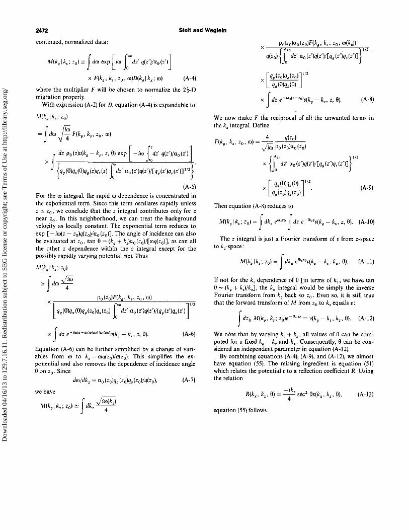
2472 Stolt and Weglein
continued, normalized data:
M(kg I ks; zo) == f dO) exp liO) 1'0 dz' q(z')/uo (Z')]
x F(kg, ks, to, O))D(kg I kx; 0)) (A-4)
where the multiplier F will be chosen to normalize the 2t-D migtation properly.
With expression (A-2) for D, equation (A-4) is expandable to
M(kg I ks; zo)
= f dw Ji: F(kg , k., zo, 0))
x f d, .,(,I,(k, - k" " 9) oxp [ - '00 1:"" q(,')fa, ("JJ {qg (O)qs (O)qg (z)qs (z) fdz' Uo (z')q(z')/[qg (z')qs (z')] 1/2 } •
(A-5)
For the 0) integral, the rapid 0) dependence is concentrated in the exponential te~m. Since this term oscillates rapidly unless z ~ Zo, we conclude that the z integral contributes only for z near Zo. In this neighborhood, we can treat the background velocity as locally constant. The exponential term reduces to exp [ - iO)(z - zo)q(zo)/uo (zo)]. The angle of incidence can also be evaluated at Zo, tan 8 = (kg + k.)uo (zo)/[O)q(zo)], as can all the othet z dependence within the z integral except for the possihly rapidly varying potential v(z). Thus
M(kg I ks; zo)
~ f dO) ~
xl r<o . J1 /2 qg (O)qx (O)qg (zo)qs (Zo) Jo dz' Uo (Z')q(Z')/(qg (z')qs (z')
x f dz e - iro(z - zo)q(zo)/oo(zo)v(k - k z 8) g s'" (A-6)
Equation (A-6) can be further simplified by a change of variables from 0) to kz = O)q(zo)/u(zo). This simplifies the expotlentiai and also removes the dependence of incidence angle 8 on Zo . Since
dO)/dkz = Uo (zo)qg (zo)qs (zo)/q(zo), (A-7)
x [qg (zo)qs (zo)] 1/2
qg (O)qs (0)
x f dz e-ik,(z-zOlv(k - k z 8) g s'" (A-8)
We now make F the reciprocal of all the unwanted terms in the kz integral. Define
q(zo) 4 F(kg,ks,zo,O))= r=
y iO) Po(zo)uo(zo)
{fZO }1/2 x 0 dz' uo (z')q(z')/[qg (z')qs (Zl)]
X [
qg. (O)qs(O) J1 /2 qg (zo)qs (zo) .
(A-9)
Then equation (A-8) reduces to
M(kg I ks; zo) = f dkz eik,zo f dz e - ik'Zv(kg - ks, z, 8). (A-lO)
The z integral is just a Fourier transform of v from z-space to kz-space:
M(kg I ks; zo) = f dkz eik'ZOv(kg - ks, kz , 8). (A-ll)
If not for the kz dependence of 8 [in terms of kz , we have tan 8 = (kg + ks)/kz], the kz integral would be simply the inverse Fourier transform from kz back to Zo. Even so, it is still true that the forward transform of M from Zo to kz equals v:
f dzo M(kg, ks; zo)e-ik,zo = v(kg - k., k .. 8). (A-12)
We note that by varying kg + k., all values of 8 can be computed for a fixed kg - ks and kz . Consequently, 8 can be considered an independent parameter in equation (A-12).
By combining equations (A-4), (A-9), and (A-12), we almost have equation (55). The missing ingredient is equation (51) which relates the potential iJ to a reflection coefficient R. Using the relation
(A-13)
equation (55) follows.
Dow
nloa
ded
04/1
6/13
to 1
29.7
.16.
11. R
edis
trib
utio
n su
bjec
t to
SEG
lice
nse
or c
opyr
ight
; see
Ter
ms
of U
se a
t http
://lib
rary
.seg
.org
/