Epithelial tissues Connective Tissues Nervous Tissues Muscle tissues.

Malardalen University Licentiate ThesisNo. 73
MICROWAVE IMAGING OF BIOLOGICAL TISSUES:
applied toward breast tumor detection
Tommy Gunnarsson
April 2007
Department of Computer Science and ElectronicsMalardalen University
Vasteras, Sweden

Copyright c©Tommy Gunnarsson, 2007ISSN:1651–9256ISBN:978–91–85485–43–7Printed by Arkitektkopia, Vasteras, SwedenDistribution: Malardalen University Press

Abstract
Microwave imaging is an efficient diagnostic modality for non-invasively visualizingdielectric properties of non-metallic bodies. An increasing interest of this field hasbeen observed during the last decades. Many application areas in biomedicine havebeen issued, recently the breast tumor detection application using microwave imag-ing. Many groups are working in the field at the moment for several reasons. Breastcancer is a major health problem globally for women, while it is the second mostcommon cancer form for women causing 0.3 % of the yearly female death in Sweden.Medical imaging is considered as the most effective way of diagnostic breast tumors,where X-ray mammography is the dominating technique. However, this imagingmodality still suffers from some limitations. Many women, mostly young ones, haveradiographically dense breasts, which means that the breast tissues containing highrates of fibroglandular tissues. When the density is very similar to the breast tumorand the diagnosis is very difficult. In this case alternative modalities like MagneticResonance Imaging (MRI) with contrast enhancement and Ultrasound imaging areused, however those are not suitable for large scale screening program. Anotherlimitation is the false-negative and false-positive rate using mammography, in gen-eral 5–15 % of the tumors are not detected and many cases have to go though abreast biopsy to verify a tumor diagnosis. At last the mammography using breastcompression, sometimes painful, and utilizing ionizing X-rays. The big potentialin microwave imaging is the reported high contrast of dielectric properties betweenfibroglandular tissues and tumor tissues in breasts and that it is a non-ionizingmethod which probably will be rather inexpensive.
The goal with this work is to develop a microwave imaging system able to re-construct quantitative images of a female breast. In the frame of this goal thisLicentiate thesis contains a brief review of the ongoing research in the field of mi-crowave imaging of biological tissues, with the major focus on the breast tumordetection application. Both imaging algorithms and experimental setups are in-cluded. A feasibility study is performed to analyze what response levels could beexpected, in signal properties, in a breast tumor detection application. Also, theusability of a three-dimensional (3D) electromagnetic-wave simulator, (QW3D), inthe setup development is investigated. This is done by using a simple antennasetup and a breast phantom with different tumor positions. From those results itis clear that strong responses are obtained by a tumor presence and the diffractedresponses gives strong information about inhomogeneities inside the breast.
The second part of this Licentiate thesis is done in collaboration between Malar-dalen University and Supelec. Using the existing planar 2.45 GHz microwave cam-era and the iterative non-linear Newton-Kantorovich code, developed at Departementde Recherches en Electromagnetisme (DRE) at Supelec, as a starting point, a newplatform for both real-time qualitative imaging and quantitative images of inho-mogeneous objects are investigated. The focus aimed to breast tumor detection.For the moment the tomographic performance of the planar camera is verified in

simulations through a comparison with other setups. Good calibration is observed,but still experimental work concerning phantom development etc. is needed beforeexperimental results on breast tumor detection may be obtained.

Swedish Summery – Sammanfattning
Mikrovagsavbildning ar en effektiv metod att avbilda en ickemetallisk kropps dielek-triska egenskaper. Detta forskningsomrade har fatt ett okat intresse under desenaste decennierna, manga tankbara medicinska tillampningar har studerats ochnu senast brostcancerdetektion med hjalp av mikrovagsavbildning. Det ar avflera anledningar som denna applikation ar intressant. Brostcancer ar ett storthalsoproblem for kvinnor globalt, dar 0,3 % av de arliga dodsfallen for kvinnori Sverige ar i korrelation till brostcancer. Medicinsk avbildning ar den effekti-vaste metoden att diagnostisera brostcancer, dar mammografin ar den dominantatekniken. Trots det sa har tekniken vissa brister. Manga kvinnor, speciellt yngre,har hoga halter av fiber och kortel vavnad, dessa vavnader har liknande densitetsom tumorer sa diagnostiken blir valdigt svar. Alternativa tekniker i detta fall arMagnetresonanstomografi (MRI) med tillfort kontrastmedel och Ultraljud. Dessatekniker ar dock inte ansedda som lampliga i storskalig brastcancerscreenings pro-gram. En annan svaghet ar felfrekvensen i diagnostiken, bade negativ och positiv,uppskattningsvis sa blir 5–15 % av cancerfallen inte upptackta och manga gangermaste brostbiopsi anvandas for att diagnostisera en brostcancer. Till sist, mammo-grafin anvander sig av laga halter av joniserande stralning och kraver brostkompres-sion, vilket ar smartsamt i vissa fall. Den stora potentiella mojligheten for mikrovag-savbildning ar den hoga kontrasten for dielektriska egenskaperna mellan brostetsfiber och kortel vavnader jamfort med tumoren och att ingen joniserande stralninganvands. Troligen skulle denna teknik aven vara ett relativt billigt alternativ.
Malet med detta arbete ar att utveckla ett avbildningssystem for mikrovagordar ett kvinnobrost kan avbildas kvantitativt. Denna avhandling tacker vissa delarav detta mal med borjan i en oversikt over pagaende forskning inom omradet,med fokus pa brosttumorsdetektion. Bade algoritmer och fullstandiga experi-mentella system behandlas. En inledande studie behandlas med fokus pa vilkensignal respons man kan vanta sig av vid brostcancerdetektion med mikrovagor.Anvandbarheten av en elektromagnetisk vagsutbredningssimulator (QW3D) vidutveckling och analys av experimentella uppstallningar undersoks. Till detta anvandesen enklare antennuppstallning tillsammans med en brastfantom dar tumoren kanplaceras i olika positioner. Resultatet visar att en tumor ger stark signal responsoch att diffraktionen ger information om inhomogeniteter inuti brostet.
Andra delen av avhandlingen ar gjord i ett samarbete mellan Malardalenshogskola och Supelec, Paris. Genom att anvanda den existerande 2,45 GHz planvag-skameran tillsammans med den iterativa och olinjara Newton-Kantorovich koden,utvecklade vid Departement de Recherches en Electromagnetisme (DRE) Supelecsom en start punkt, kan en ny plattform for undersokning av inhomogena objekttas fram. Dar bade kvalitativavbildning i realtid och kvantitativavbildning kananvandas med en fokus mot detektion av brostcancer. Planvagskameran pavisargod tomografisk formaga i simuleringar, i en jamforelse med andra uppstallningar.Bra kalibrering har astadkommits mellan algoritmen och experimentella uppstalln-

ingen, men fortfarande kravs en del arbete runt den experimentella uppstallningenoch brostfantomen for att experimentella resultat av brostcancerdetektion ska kunnauppnas.

Acknowledgments
The moment of this Licentiate thesis feels like a short break of an ongoing journeyand gives a possibility to reflect about my first part of the journey. Indeed it hasbeen hard moments with a lot of hard work, but also delighted moments solvingchallenging questions into challenging situations. In general I see this period of mylife as a huge progress, not only on a professional plane but also personally. In myreflection many supporting personalities appears in form of colleagues, my familyand friends. I would like to thank those persons who made this journey possible,who courage me to continue and supporting me through the hard moments of thisjourney.
Hans Berggren (former head of the department) and Prof. Ylva Backlund (mainsupervisor) thank you for offering me the possibilities to do my Ph. D. studies inthis field. I’m also grateful for my supervisor Denny Aberg who supported methrough many discussions and in my decision to focus in the algorithmic part andalso for my visit to Supelec, I wish you good luck at your new position in theindustry. I also want to thank my external supervisor Hans Skold mainly for yoursupport at the beginning of my journey and to open up the possibilities to doexperiments at Saab Metech. I am thankful to: Mats Karlsson and Ulf Eriksson atSaab Metech who gave us free support and usage of the experimental equipments.P. O. Risman for your interesting discussions about microwaves and your supportin the beginning of my journey. Nils-Fredrik Kaiser for your motivation and spiritand putting me in contact with prof. Jean Charles Bolomey. Danel Noreland foryour lectures and discussions around the the inverse problem in microwave imaging,without your help my journey would be hard to finish.
I’m more than grateful to: Prof. Jean Charles Bolomey who offered me to stayat Supelec during 6 months in 2006 for collaboration, also for being my Frenchmain supervisor in my continuing journey as a divided Ph. D. student betweenMalardalen University and University Paris SYD VI, Supelec. Alain Joisel andNadine Joiachimowicz who gave me great support during my stay with many in-teresting discussions and taking the role as assistant supervisors. This period wasprobably the most fruitful during my preparations of this thesis, without your helpmy thesis would not have the format it has today. I’m looking forward to continuethis work in the near future. I also want to thank the other colleges at Supelecwho helped me to get along in Paris, in everything from running exercise to morespecific professional discussions around microwave imaging.
I am thankful to the Swedish Knowledge Foundation for founding this part ofmy journey also to the Royal Swedish Academy of Science for providing me a grantfor my stay at Supelec in 2006. I will also take the opportunity to thank the SwedishInstitute for selecting me for the French government grant through CNOUS, as aresult they will provide me a grant for my continuing studies at Supelec in 2007.

Ann Huguet I am grateful for your help completing the applications with yourexperienced advises.
Also thanks to my former and new colleagues at the department, especiallyPeder Norin who was my companion since the first week at the university. We wenttrough the four years studies to a Master of Science and then trough our first jobas engineer to follow up starting our Ph. D. studies together. It was always nice tohave a friend nearby, I wish you all luck in the future! I also want to thank Ali Fardand Tord Johnson who was supervising me through my Master thesis and later wasa great support trough the beginning of the journey, with many discussion aboutthe life as a Ph. D. student.
I want to thank my friends outside the office especially Andreas Ahlin who wasmy ”base camp” in Vasteras during periods when I moved back and fourth to Paris.Also, to my other friends who still are available when a far distance separating us.I want to give my largest gratitude to my parents, you have always supporting mein what I am doing and believing in my capability, without your support I wouldnever have the courage to go for what I am believing in. Also my sister who sup-porting me when I need and put my two wonderful nephews Emma and Erik intolife, those helps me to get back to life when it is too much microwaves in my mind.
Late night in Paris, April 2007.
/Tommy

Contents
1 Motivation 11.1 Scope of this work . . . . . . . . . . . . . . . . . . . . . . . . . . . . 31.2 Publications Included in the Thesis . . . . . . . . . . . . . . . . . . . 31.3 Other Related Work . . . . . . . . . . . . . . . . . . . . . . . . . . . 41.4 Summary of Appended Papers . . . . . . . . . . . . . . . . . . . . . 41.5 Author’s Contribution in the Included Publications . . . . . . . . . . 51.6 Thesis Organization . . . . . . . . . . . . . . . . . . . . . . . . . . . 5
2 Introduction 72.1 A Brief Overview . . . . . . . . . . . . . . . . . . . . . . . . . . . . . 8
2.1.1 Breast Tumor Detection Using Microwave Imaging . . . . . . 102.2 Dielectric Properties of Human Tissues . . . . . . . . . . . . . . . . . 10
3 Image Reconstruction Algorithm 153.1 Physical Description . . . . . . . . . . . . . . . . . . . . . . . . . . . 16
3.1.1 Wave Equation . . . . . . . . . . . . . . . . . . . . . . . . . . 163.2 Direct Problem . . . . . . . . . . . . . . . . . . . . . . . . . . . . . . 163.3 Non-Linear Inverse Problem . . . . . . . . . . . . . . . . . . . . . . . 19
3.3.1 Newton-Kantorovich . . . . . . . . . . . . . . . . . . . . . . . 193.4 Open Configuration Newton-Kantorovich Algorithm . . . . . . . . . 22
4 Detection of Breast Tumors 234.1 Experimental and Simulation Setup . . . . . . . . . . . . . . . . . . 254.2 Responses due to a Tumor Presence . . . . . . . . . . . . . . . . . . 26
5 Quantitative Imaging with a Planar Camera 315.1 Experimental setup . . . . . . . . . . . . . . . . . . . . . . . . . . . . 325.2 Quantitative Images of Inhomogeneous Objects . . . . . . . . . . . . 355.3 Calibration . . . . . . . . . . . . . . . . . . . . . . . . . . . . . . . . 37
6 Concluding Remarks 416.1 Future Research . . . . . . . . . . . . . . . . . . . . . . . . . . . . . 42
i

ii CONTENTS

Chapter 1
Motivation
Today, cancer is a major health problem in the society. Swedish statics reporttumors as the second most common cause of death [1], after diseases in circulationorgans. 25% of the yearly deaths are caused by tumors, where breast cancer is themost common tumor among women with around 30 caused deaths in a population of100,000. Similar numbers has been reported in North America, Europe, Australia,Polynesia and Western Africa [2], In a worldwide basis breast tumor is by far themost frequent tumor among women with 23% of all cancers. In 2002, 1.15 millionnew cases where reported, giving the rank second overall after lung cancer whenboth sexes are considered.
Worth noting, the survival rate of breast cancer is 65% in a global average [2],for a period of five years after the first detection. So breast cancer has a rather goodsurvival rate compared to other tumor forms. One reason is probably the majorscreening programs carried out in high developed countries, established to findearly invasive tumors. However, still breast tumors are the leading cause of tumormortality for women, 411,000 annual deaths was reported in 2002 [2]. Incidencerates of breast cancer are increasing in most countries, and the grown are usuallygreatest where rates were previously low. With an estimated growth about 3 %growth in East Asia and 0.5 % in the rest of the word, the world total in 2010would be 1.5 million [2]. By only looking at those numbers all research in this areaare strongly motivated.
The motivation for major screening programs is the strong correlation betweenthe outcome of a breast tumor and its size at the time of detection. Michaelsonet. al. are able to calculate the chance of survival from the size of the tumor,independent of detection method [3]. In the most high developed areas of the worldall women goes through this program with frequent radiology visits.
Today, imaging techniques takes an important role in the detection of malig-nant breast tumors, where X-ray mammography is the dominant technique. X-raymammography fulfill almost all requirements to be an efficient imaging tool. An
1

2 CHAPTER 1. MOTIVATION
imaging tool must have high specificity and sensitivity to malign breast tumors,resource effective in manpower, money and time and should also be non-invasiveand harmless [4]. Today, X-ray mammography is widely used and in general anaccepted method. However, mammography suffers from several limitations. Thesensitivity in false rate has been reported by Elmore et. al. [5] and by Huynh et.al. [6]. X-ray mammography has a false-positive rate between 2.8% to 15.9% anda false-negative rate between 4% to 34%. The false rate is mainly dependent of theexperience of radiologist. Also the specificity has a reported limitation, during theextensive mammography screening programs often, (10-50%) [7], patients needs abreast biopsy to verify the findings on the mammogram. The general number ofundetected breast tumors is estimated to be between 5% to 15% [5, 6]. One majorreason of the this high rate is the difficulty to image breasts with highly content offibrous and glandular tissues, radiographically dense breasts [7]. In this case a verylow contrast is achieved between the malign breast tissue and the fibroglandulartissues using X-ray mammography [6, 8], and alternative imaging techniques mustbe used [7].
Beside of those detection limitations, mammography uses ionizing X-rays andneeds in some cases a painful breast compression. The radiation is kept on lowlevels in today’s mammography equipments, but there is still a small risk thatthe exposure of ionizing rays producing breast cancer. Women passing an X-raymammography screening during 10 years has an estimated rate of mortality of eightout of 100,000 women [9]. However, this is still a quite high number compared tothe total risk of mortality due to breast tumor.
Complementary non-ionizing imaging methods exists today, the most importantones are Ultrasound imaging and Magnetic Resonance Imaging (MRI) with contrastenhancement. However, no one of those techniques are suitable for large scalescreening programs. They have taken an important role in the later diagnosticsto verify the malignity of the breast tissue and in situations of dense breasts [7].Other imaging techniques has a very small role in breast tumor detection today.
At the moment the highest breast tumor detection rates are reported in thehigh developed areas around the world, where the screening programmes has beenestablished [2]. However, in many areas in lower developed countries, in e.g. Africa,reporting similar rates of mortality from breast tumor while the detection is fairlylow compared to high developed contrives. Therefore, a cheap and high specificityand sensitivity solution must be found to solve the global mortality from breasttumors.
From this discussion its clear that there is a high need of complementary and/or alternatively imaging modalities in order to decrease the the global mortalityrelated to breast tumors. Microwave imaging may be one of the needed imagingmodalities in the future, at least for two reasons. First, high dielectric contrast isobserved between malignant breast tumor tissues and fibrous and glandular breasttissues in the microwave spectrum, microwave imaging has a strong potential todetecting tumors [10, 11, 12, 13, 14, 15, 16]. Second, after major research efforts of

1.1. SCOPE OF THIS WORK 3
different groups microwave imaging is generally an efficient imaging modality fornon-invasively visualizing complex dielectric properties[17, 19, 20, 21]. Those rea-sons settle a very interesting knowledge platform to establish new imaging modali-ties using microwaves applied toward breast tumor detection. A microwave imagingsystem will probably be a very inexpensive solution compared to MRI and X-rayComputed Tomography (CT) enabling a wide usability.
1.1 Scope of this work
The work included in this Licentiate thesis was initiated during the establishmentof the microwave imaging research at the Department of Computer Science andElectronics at Malardalen University. The work can be divided into two parts.One initiative part, where a feasibility study covering the responses obtained by atumor inside a breast phantom and the second part covering quantitative microwaveimaging in breast tumor detection, using the planar 2.45 GHz camera and theiterative Newton-Kantorovitch algorithm.
From the initial feasibility study the responses due to the tumor presenceare observed in amplitude and phase responses without imaging algorithms in-cluded. Also, the usability of a commercial Finite Difference Time Domain (FDTD)electromagnetic-wave simulator (QW3D) in the development stage of an imagingsetup was investigated. Trough contact with Prof. Jean Charles Bolomey collabo-rated studies was investigated. At first an investigation about microwave imagingalgorithms has been experienced, in this context a review of the existing imagingsystems and algorithms is contributed. As an result of the review the planar 2.45GHz camera seems to be an interesting and quick choice for quantitative imagingstudies in breast tumor detection. The usage of an extended version of the Newton-Kantorovich code, developed by Joachimowicz et. al., the later part of this thesishas been carried out to obtain quantitative image reconstruction of inhomogeneousobjects using the planar microwave camera with focus on the breast tumor detec-tion application. This was done in a collaboration between Malardalen Universityand Supelec.
1.2 Publications Included in the Thesis
Paper A - T. Gunnarsson, Microwave Imaging of Biological Tissues: the currentstatus of the research area,” Technical report, Malardalen University, Departmentof Computer Science and Electronics, Dec. 2006
Paper B - D. Aberg, T. Gunnarsson, P. Norin, “Steps to Microwave Probingof Complex Dielectric Bodies,” IEEE 48th International Midwest Symposium onCircuits and Systems (MWSCAS), Cincinnati, OHIO, USA, Aug. 2005.

4 CHAPTER 1. MOTIVATION
Paper C - T. Gunnarsson, N. Joachimowicz, A. Diet, C. Conessa, D. Abergand J. Ch. Bolomey, “Quantitative Imaging Using a 2.45 GHz Planar Camera,” Accepted for proceeding, 5th World Congress on Industrial Process Tomography,Bergen, Norway, 3rd-6th Sep. 2007.
1.3 Other Related Work
Paper D - P. Norin, T. Gunnarsson, D. Aberg, P. O. Risman, “MICROWAVEPROBING OF COMPLEX DIELECTRIC BODIES,” 13th Nordic Baltic Confer-ence Biomedical Engineering and Medical Physics, pp. 203–204, 13th–17th June,2005.
Paper E - T. Gunnarsson, N. Joachimowicz, A. Joisel, J. Ch. Bolomey, “Com-parison Between a 2.45 GHz Planar and Circular Scanners for Biomedical Appli-cations,” Extended abstract accepted for proceeding, International Conference onElectromagnetic Near-Field Characterization and Imaging (ICONIC), St. Louis,Missouri, USA, 27th–29th June, 2007.
1.4 Summary of Appended Papers
Paper A - This review report covers the current research in the field of microwaveimaging of biological tissues, both the complete experimental imaging systems andthe algorithm development are covered. The purpose of this study is to investigatethe usability of the planar 2.45 GHz camera and the Newton-Kantorovich algo-rithm, developed at Departement de Recherches en Electromagnetisme (DRE) atSupelec, for quantitative imaging for breast tumor detection.
Paper B - This paper presents a feasibility study in breast tumor detection usingmicrowaves. Using a water-filled metallic container with three attached waveguideantennas, 90◦ in between them, the response from a 10 mm diameter tumor insidea breast phantom is measured and investigated using a network analyzer. Themeasured results are also compared with simulated result generated by a FDTDwave simulation tool, QW3D. The result is comparable after some calibration andthe conclusion is that the FDTD simulator is a very useful tool to investigate theimaging setup in the development phase. Also, the tumor was detectable from the11 dynamic responses of the measured signals, but an imaging algorithm must beapplied to get the information about position and size information and a quantita-tive imaging algorithm must be used to verify the properties of the tumor.
Paper C - In this paper a simulation comparison between three different mi-crowave imaging setups for breast tumor detection is presented. The ability to per-form quantitative images using an open configuration based Newton-Kantorovich

1.5. AUTHOR’S CONTRIBUTION IN THE INCLUDED PUBLICATIONS 5
algorithm is verified. The same algorithm is used with different input parametersdescribing the configuration of the different setups. In the comparison differentsignal to noise ratios (SNR) are considered, by applying a Gaussian noise distribu-tion, to analyze the stability of the algorithm for the different setups in a realisticsituation. The setups used are one planar setup and two circular setups corre-sponding to exisitng experimental setups [10, 39, 63]. This paper also includes theexperimental result performed with the planar 2.45 GHz camera at Departementde Recherches en Electromagnetisme (DRE) at Supelec. The goal is to performquantitative images for breast tumor detection using experimental data. This isthe first attempt to perform quantitative images of inhomogeneous objects withthe planar camera. This paper includes a discussion about the difficulties to obtainhigh precision calibration for quantitative results.
1.5 Author’s Contribution in the Included Publi-cations
Paper A - The only author of the state of the art review report.
Paper B: A major part of the simulation study concerning the dynamical responsedue to the tumor presence. Some parts of the measurements and the calibrationbetween measurements and simulations. Also, some parts of the manuscript writingand performed the presentation on the conference.
Paper C - A major part of the general idea in the paper and the first authorof the manuscript. Extending the existing Newton-Kantorovich algorithm to a thegeneral open setup configuration version and performed the simulations. Part ofthe experimental work with calibration using reference objects.
1.6 Thesis Organization
The organization of this thesis is as follows. A brief introduction to microwave imag-ing is presented In Chapter 2. From the general idea to a review of other groupscontributions, until recent. Both complete imaging systems and algorithms is cov-ered with focus on the breast tumor detection application, based on paper A. Also,the dielectric properties of the human body will be briefly reviewed. In Chapter 3the imaging algorithm used herein is described, based on the Newton-Kantorovitchcode developed by Joachimowicz et. al. The method will briefly described togetherwith the extension to support an open configuration solution, used in paper C.Chapter 4 covering the feasibility study of breast tumor detection in paper B,with aim on the responses due to a tumor presence inside a breast a discussionabout what parameters effecting the response levels and the delectability without

6 CHAPTER 1. MOTIVATION
an imaging algorithm included. In Chapter 5 the planar 2.45 GHz microwave cam-era is used for quantitative imaging of inhomogeneous objects concerning the breasttumor detection application. The tomographic ability of the geometry is verifiedin a simulation comparison with two other circular setups, presented in paper C.Also, the calibration used for quantitative image reconstruction is described therein.The conclusion and the expected future work is presented in Chapter 6. Finally,the appended papers are collected in the last part of this thesis.
Chapter 2
Introduction
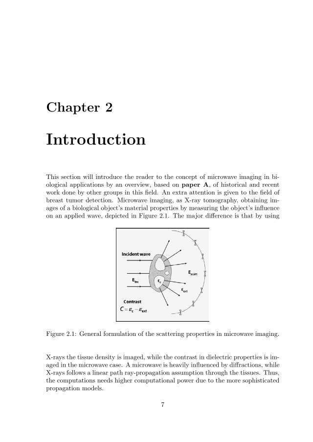
This section will introduce the reader to the concept of microwave imaging in bi-ological applications by an overview, based on paper A, of historical and recentwork done by other groups in this field. An extra attention is given to the field ofbreast tumor detection. Microwave imaging, as X-ray tomography, obtaining im-ages of a biological object’s material properties by measuring the object’s influenceon an applied wave, depicted in Figure 2.1. The major difference is that by using
Figure 2.1: General formulation of the scattering properties in microwave imaging.
X-rays the tissue density is imaged, while the contrast in dielectric properties is im-aged in the microwave case. A microwave is heavily influenced by diffractions, whileX-rays follows a linear path ray-propagation assumption through the tissues. Thus,the computations needs higher computational power due to the more sophisticatedpropagation models.
7

8 CHAPTER 2. INTRODUCTION
2.1 A Brief Overview
The opening of microwave imaging in biomedical applications were performed byLarsen and Jacobi et.al. in the late 70s, developing a water-immersed antenna forbiomedical applications [22]. This was the first time someone was able to penetratean biological object with microwaves, (due to the wave impedance matching be-tween the water and the human body), to create images of the internal structures.Images was obtained of the internal structure of a Canine kidney from the trans-mission coefficients between two rotated antennas [23]. From those results a majorinterest have been focused on microwave imaging in biomedical applications [24],the initial focus was on remote measurements of internal temperature. The dielec-tric properties of biological tissues are highly temperature dependent, which makesmicrowave imaging a promising method to control the effect during microwave hy-perthermia treatment [25, 26, 27, 28]. Semenov et. al. has been focusing on isfinding heart disease like ischemia and infarction [29, 30]. The most recent appli-cation is breast tumor detection using microwave imaging, the initial and majorcontribution has been done by Meaney et. al. [10, 17, 18, 31]. Recently many othergroups are working in this application area [11, 12, 13, 15, 32, 33].
The two major approaches of microwave imaging today are tomographic meth-ods where cross-sectional slices of the dielectric properties is generated and radarapproaches where strong scatterers is found inside an object using radar techniques.The radar approach is not issued in this thesis, but a recent review of the techniqueis published by Hagness et. al. [34]. The tomographic methods are based on the in-verse scattering problem and will be divided into two different groups in this thesis.First, the diffraction tomography, a linear approach, which uses Born or Rytov ap-proximations. This method is a very computation efficient method obtaining quasireal-time imaging [27, 35, 36, 37]. In situations of small objects with a low contrastwith respect to the background medium this is a very efficient method. In a situa-tion of larger objects with large contrast to the background medium this method isnot useful [38]. This is the case in the most situations of biomedical applications,where an non-linear method is needed. However, still the diffraction tomographyformalization may be used in spectral domain to obtain real-time images of theequivalent currents inside the object [39].
The second group, a non-linear deterministic approach was first introduced byJoachimowicz et. al. and Chew et. al. in the beginning of the 90s [19, 40].Also, Caorsi et. al. made early contributions in this domain [41]. The methodis based on iterative optimization of an object function using a Newton based orConjugate Gradient based scheme. Non-linear inverse problem in microwave imag-ing has interested many groups [12, 13, 33, 42, 43, 44, 45, 71]. The algorithmhighly computational heavy, therefore mainly two-dimensional (2D) imaging hasbeen used, however, some efforts have been initiated in the three-dimensional (3D)case [19, 46, 47, 48, 49]. Another computation saving approximation used is theinfinity approximation of the coupling medium, which means that the interaction

2.1. A BRIEF OVERVIEW 9
between the antennas, surrounding covering and the object are ignored. This ap-proximation is very useful as long the background medium is lossy, like water. How-ever the antenna interaction has been implemented in some cases [50, 51, 52, 53].
Recently alternative optimizing schemes have been reported, the MultiplicativeRegularization Contrast Source inversion by Abubakar et. al. [49, 54, 55], globaloptimization methods using neural networks, genetic algorithms and nondestructiveevaluation by Caorsi et. al. [56, 57, 58, 59]. These methods avoid local minima,however at the cost of a slower convergence and higher computation load. Until nowsingle frequency solutions are most widely used, but different groups are workingon multi-frequency solutions [12, 33, 60]. It is known that the low frequencies lowerthe effect of phase non-linearities and stabilize the algorithm, while the higherfrequencies increase the resolution, and the idea is that a combination will improvethe reconstruction. However, the frequency dependence of biological tissues is adifficulty in this approach and probably many future research efforts could focus inthis area.
Many experimental setups have been developed since the beginning of the 80s.One of the first and still running, the planar 2.45 GHz microwave camera devel-oped by Bolomey et. al. [25, 35] This camera using a quasi-plane wave as incidentfield and measure the field on a vertical plane of 1024 sensors behind the object.This system makes real-time acquisition using the Modulated Scattering Technique(MST) [39, 61]. Franchois et. al. was able to create quantitative images of homoge-nous objects with this equipment in the 90s [62]. The next break though was the64 antenna circular 2.33 GHz camera developed by Jofre et. al. in the beginningof the 90s [27, 63]. Using this system a 2D cross-section of a human arm was re-constructed [20], and the circular experimental geometry was proven to be a betterchoice for 2D imaging [27, 64]. Since then other groups have followed this trend[12, 28, 29, 65, 66]. The first wide-band system was developed by Meaney et. al. inthe middle of the 90s, a circular monopole antenna system with a frequency rangebetween 0.3-1.2 GHz [65].
More recently Persson et. al. has developed a similar system utilizing a fre-quency band between 2 − 7 GHz [12], for data acquisition used in a time-domainmulti-frequency imaging algorithm. Semenov et. al. has developed experimentalsetups able to perform fully 3D acquisition [67, 68, 69, 70], probably the majorfuture efforts will be focused in this domain, while slicing a strongly 3D dependentobject using 2D models gives many artifacts [29, 71]. The planar 2.45 GHz cameradeveloped by Bolomey et. al. is able to measure the vertical-polarized field at1024 points on a vertical plane behind the object, in real-time [39]. Therefore, thiscamera is highly interesting as an efficient acquisition tool measuring 3D data fora quasi-3D algorithm [47] or fully 3D using an updated version of the camera, ableto measure the two-component vectorial field. Note, the Newton-Kantorovich algo-rithm generalized to the 3D, developed by Joachimowicz et. al., may be potentialstarting point for 3D quantitative imaging [19, 72].
In a Malardalen University and Supelec cooperation a solid experimental plat-
10 CHAPTER 2. INTRODUCTION
form for 3D analysis of inhomogeneous objects may be developed based on extendedversions of the Newton-Kantorovich algorithm and the planar camera. Franchois et.al. has shown promising results for quantitative imaging of 2D homogenous objectsusing the planar camera [62]. The next step is to perform quantitative inhomoge-neous 2D objects before starting a quasi-3D imaging. Another big advantage withthe planar camera is the already implemented real-time algorithm in spectral do-main, this algorithm reconstructing the equivalent currents in vertical planes usingthe filtered-backpropagation process. Using this algorithm field behaviors insidethe object may be observed in real-time.
2.1.1 Breast Tumor Detection Using Microwave Imaging
Today, a major focus is applied on the breast tumor detection application usingmicrowave imaging. The major reason for this is the potentially high dielectriccontrast between cancerous tissues and normal breast tissues [11, 12, 75]. A majorcontribution comes from the two groups Meaney et. al. and Hagness et. al.,reviewed in [14, 16]. They are using two different approaches Meaney et. al. using aHybrid Element (HE) method in a non-linear inverse scattering formulation [42, 43],while Hagness et. al. using a radar approach [11, 34].
The first imaging system to perform quantitative images of breast phantoms[17, 44] was developed by Meany et. al. [10]. Even real breasts were imaged usinga clinical prototype developed in the 2000s [10]. Hagness et. al. has verified theirradar approach in an experimental setup using a ultra-wideband antenna [11, 73],with impressive results. However, in a realistic situation it will be very hard todiagnostic a tumor while the method just obtains qualitative images. The solutionmay be to use statistical methods to verify the result [74]. Otherwise, a quantitativemethod must be used, like Meaney et. al. Note, the difference between a qualitativeand a quantitative image is that the quantitative image gives information directlycorrelated to the dielectric properties.
More recently, other groups has joined this field [12, 13, 32, 33] etc. Miyakawaet. al. has investigated the usability if their developed linear chirp pulse microwavecomputed tomography algorithm (CP-MCT), [76, 77, 78], to the breast tumor de-tection application [32]. Fhager et. al. developing a time-domain nonlinear inversescattering algorithm for multi-frequency focused on imaging systems for breast tu-mor detection [12, 12]. Also, a linear chirp pulse algorithm has been implementedby this group [12, 79].
2.2 Dielectric Properties of Human Tissues
In this section the dielectric properties of human tissues will be introduced, whichmust be known to understand the properties of quantitative microwave imaging.This section gives a brief description of the definition and the widely used models

2.2. DIELECTRIC PROPERTIES OF HUMAN TISSUES 11
for the dispersion, (frequency dependance), of the tissues. At last typical numbersof the dielectric properties will be given, together with tissues concerning the breasttumor detection application.
In quantitative microwave imaging the dielectric properties is reconstructed re-garding the differences in the complex permittivity, while non-metallic materialsare considered in biomedical applications, defined by Equation (2.1).
ε∗ = ε′ − jε′′, (2.1)
where ε′ is the relative permittivity describing the polarization effects of chargedparticles in the tissue and ε′′ describing the out-of-phase losses due to the dis-placement currents generated by the applied electromagnetic field. Considering thebiological tissues as dielectrics the losses often are described by the conduction σ,which is approximated to the displacement current effect only, as Equation (2.1),[80].
σ = 2πfε0ε′′, (2.2)
where the permittivity of free space is defined ε0 = 136π 10−9 and f is the frequency.
The electrical properties of the human body has interested researchers since thebeginning of the 20s century, where Schwan et. al. dominated the field of physicalinteraction between electromagnetic field and dielectric properties of tissues. Fosterand Schwan published a critical review concerning the physical mechanisms behindbiological tissues dispersion in dielectric properties [80]. The dielectric properties ishighly dispersive due to the cellular and molecular relaxation, generated by differentparts of the tissues at different frequencies. In the microwave region the dominantrelaxation is the dipolar relaxation of free water molecules. Therefore, the dielectricproperties of the tissues in microwave region are highly correlated to the watercontent.
More recently, Gabriel et. al. made a major review of measured dielectricproperties together with own measurements on healthy human tissues, with thefinal goal of physical modeling of human tissues for frequencies between 10 Hz–100 GHz [81, 82, 83]. The basic and well known model is the Debye expression inEquation (2.3), [83].
ε∗(f) = ε∞ +εs − ε∞
1 + j2πfτ, (2.3)
where ε∞ is the permittivity at frequencies 2πfτ � 1, εs the permittivity at 2πfτ� 1 and τ is the time constant of the relaxation mechanism in the tissue. Toenable a more wide-band model of the properties the time constant can be dividedin several regions to match different type of relaxation as
ε∗(f) = ε∞ +εs − ε2
1 + j2πfτ1+
ε2 − ε∞1 + j2πfτ2
[84]. (2.4)
Note, the permittivity properties ε∞ and εs must also be divided in the same regionsby adding intermediate values. However, due to the complexity of the structure

12 CHAPTER 2. INTRODUCTION
and composition of biological tissues Gabriel et. al. used an extended Cole–Coleexpression, defined in Equation (2.5), [83].
ε∗(f) = ε∞ +∑
n
∆εn
1 + (j2πfτn)1−αn+
σi
j2πfε0, (2.5)
where σi is the static ionic conductivity by a constant field influencing very lowfrequencies. Equation (2.5) was successfully used in a wide frequency band between10 Hz–100 GHz by individually choosing the parameters for different tissues [83].The result for different human tissues at 2.5 GHz are presented in Table 2.1.
Tissue ε′ σ(S/m)Blood 56 - 60 2.5Bone 12 0.4
Brain (Grey matter) 45 2Fat (Not infiltrated) 4 - 5 0.07 - 0.1
Heart 55 2.3Kidney (Cortex) 55 2.5
Liver 42 1.8Lung (Inflated) 20 0.7 - 0.8
Muscle 50 - 55 1.8 - 2.2Skin (Dry) 38 1.5Skin (Wet) 43 1.8
Spleen 52 2.2Tendon 42 1.8
Table 2.1: Approximate properties of human tissues determined by Equation (2.5)for frequency of 2.5 GHz, verified with measurements [81, 82, 83].
Also, the female breast tissues have been studied, with focus on the breasttumor detection. Ex vivo measurement of fresh human malignant and normalbreast tissues has been performed by several groups. Chaudhary et. al. between3 MHz–3 GHz [85], Surowiec et. al. between 20 kHz–100 MHz [86], Campbellet. al. at 3.2 GHz [87] and Joines et. al. between 50 MHz–900 MHz [88]. Theconclusion from those measurements is a significant contrast between malignanttissues and normal breast tissues, approximately 4:1 in permittivity and between4–8:1 in conductivity along the frequency band of microwaves. The measured valuesdiffers significantly between different patients due to both measurement difficultiesand the rate of fibroglandular tissues, as shown in Table 2.2. Moreover, this contrastseems to be slightly overestimated while the dielectric properties of the tissues arechanged when they are removed, due to changes in blood flow, water content and themetabolism is interrupted [80]. During in vivo measurements this contrast seems tobe closer to 2:1 in permittivity and 3:1 in conductivity, according to tomographic

2.2. DIELECTRIC PROPERTIES OF HUMAN TISSUES 13
Tissue ε′ σ(S/m)Normal Tissue 10 - 25 0.35 - 1.05
Fat 4 - 4.5 0.11 - 0.14Tumor (Malignant) 45 - 60 3.0 - 4.0
Tumor (Benign) 10 - 50 1.0 - 4.0
Table 2.2: Measured dielectric properties of ex vivo female breast (2 – 3.2 GHz),[85, 87].
breast images using a clinical prototype, by Meaney et. al. [10]. From thoseresults ε′=30–36 and σ=0.6–0.7 S/m seems to be a more appropriate estimationof normal female breast tissues at 900 MHz. Recently, Hagness et. al. issuing theneed of extended measurements of the dielectric properties of female breasts andcollaborative efforts initiated between the University of WisconsinMadison and theUniversity of Calgary to obtain measured data of female breast tissues. However,they proposing an expected dielectric contrast between 2–5:1 between malignantand normal breast tissues.

14 CHAPTER 2. INTRODUCTION
Chapter 3
Image ReconstructionAlgorithm
As presented in paper A, there are in general two different approaches to createan image with microwaves, by using radar techniques or using a tomographic for-mulation. In this thesis the tomographic methods is used, for information aboutthe radar approach the reader may look into the work done by Hagness et. al.[11, 15, 73]. The tomographic method is divided in two different groups in thischapter, diffraction tomography and non-linear inverse scattering.
The diffraction tomography was the first attempt to create quantitative imagesusing microwaves [27, 35, 36, 37]. The method tries to reconstruct the equiva-lent currents inside the object, which generating the received scattered field. Theequivalent currents are dependent by both the field inside the object and the com-plex permittivity of the object. In the reconstruction process both those termsare unknown, while measuring only the scattered field outside the object. By ap-proximating the field inside the object to the incident field without concerning theinfluence of the object, (the influence of the object is much lower compared to theincident field), the complex permittivity can be found. This approximation is calledthe Born approximation [38] and may easily be implemented for quasi real-time ap-plications. However, when the object are larger or have a high contrast the Bornapproximation is not valid and only a qualitative result is obtained [27, 38].
To obtain quantitative images of larger high contrast objects a non-linear inversescattering method has to be used. In this case the total field inside the object isconsidered, with the object’s interaction included.This is a non-linear phenomenonsolved by iteratively solving a linear direct problem. Different approaches have beenused but most of them are based around a non-linear least square optimization.
The inverse scattering code developed by Joachimowicz et. al. in the beginningof the 90s was used as a startup point in this Licentiate thesis. This code based on
15

16 CHAPTER 3. IMAGE RECONSTRUCTION ALGORITHM
Newton-Kantorovich process gives a 2D single frequency solution [19, 20]. (This isvery similar to the Levenberg-Marquardt method more common in the literature[62, 64]). The formulation may be divided in three parts, the physical description,the numerical direct problem and the iterative non-linear optimization.
3.1 Physical Description
Maxwell’s equations are the fundamental basis physically describing any electro-magnetic (EM) wave propagation problem [89, 90], thus the starting point for theinverse scattering formulation. The Maxwell’s equations describe the field proper-ties along all three dimension axes, which results in a calculation heavy vectorialproblem. By knowing the scenario several simplification may be done to the finalwave equation, describing the propagation, e.g. considering vertical polarizationand non-magnetic material.
3.1.1 Wave Equation
A common wave equation is the scalar Helmholtz’s equation describing the time-harmonic electric field in a situation, where the incidence field is a vertically polar-ized and the object properties is homogenous along the vertical z-axis. The problemis then transformed into a 2D problem, defined by Equation (3.1), [40, 41, 43].
(∇2 + k2(r))e(r) = 0, (3.1)
where k is the wavenumber of the electromagnetic (EM) wave containing the di-electric properties of the medium of propagation. The e(r)-term is the total electricfield, i.e. including interactions of an object.
3.2 Direct Problem
Solving the direct problem gives the computed field at the receiving points, whichis the result of the interaction between a known object and incident field fromthe transmitting point. Figure 3.1 shows the geometry for a 2D case, where thetransmitter can be modeled by an incident plane wave or a source of cylindricalwaves with vertical polarized E-field along the z-axis. The object has an estimatedcomplex permittivity ε∗ and the receiving points may be arranged along a linebehind or along a circle around the object.
Several different methods can be used to implement the wave equation into thedirect problem. From the review in paper A, often used methods are the integralformulation using Method of Moments (MoM) [19, 40, 41, 62, 64, 91], Finite ElementMethod (FEM) in hybrid with the Boundary Element (BE) formulation [10, 42, 43]or in some cases Finite Difference Method (FDM) [33, 47].

3.2. DIRECT PROBLEM 17
Figure 3.1: Two-dimensional TM-model in the forward problem, (a) planar setup,(b) circular setup.
The formulation used in this thesis is based on the integral formulation of thescalar Helmholtz’s equation using MoM. The total field ev(r) in Equation (3.1) isassumed to be the sum of the incident field ei
v (without an object) and the scatteredfield es
v(caused by the object), according to Equation (3.2).
ev(r) = eiv(r) + es
v(r), (3.2)
where the notation v indexing the view in a multi-view process by rotating thereceivers. The incident field ei
v is assumed as the homogeneous solution of theHelmholtz’s equation without object and the scattered field is the solution of theinhomogeneous Helmholtz’s equation defined in Equation (3.3). In this case theobject is described as a number of small source points generating the scattered fielddefined by the Dirac delta function in the right side of Equation (3.3).
(∇2 + k1)G(r, r′) = −δ(r − r′), [38]. (3.3)
Note, that the index r represent the observation points, (the receiving antennas),while r′ represents the source point inside the object region. The term G(r, r′) repre-sent the two-dimensional Green’s function, defined as G(r, r′) = −j/H
(1)0 (k1|r−r′|)
with the the zero order Hankel function of the first kind. The k1-term is thewavenumber of the background medium. The Dirac delta function can be definedas the equivalent currents Jv inside the object generated by the contrast of thecomplex permittivity C(r′) between the object and the total field ev(r′) inside theobject region as defined in Equation (3.4).
Jv = C(r′)ev(r′), [41]. (3.4)

18 CHAPTER 3. IMAGE RECONSTRUCTION ALGORITHM
Where,C(r′) = k2
obj(r′)− k2
1, (3.5)
andk2
obj(r′) = ω2µ0ε
∗(r′) (3.6)
k21 = ω2µ0ε
∗1 (3.7)
Note, the difference of the two wavenumbers is the complex permittivity ε∗ ofthe object and the surrounding medium [36]. By inserting Equation (3.4) into (3.3)gives the solution of the scattered field es
v(r) in form of a convolution in the integralformulation as Equation (3.8).
esv(r) =
∫∫S
G(r, r′)C(r′)ev(r′)dr′ (3.8)
By inserting Equation (3.8) in (3.2) gives the following linear system for the totalfield
eiv(r) = ev(r)−
∫∫S
G(r, r′)C(r′)ev(r′)dr′ (3.9)
The integral formulation ,in (3.8), is transformed into a discrete version using MoM[19, 40, 41, 64, 89], Equation (3.10).
esv(rm) =
N∑j=1
G(rm, rj)C(rj)ev(rj), m = 1, 2, · · ·,M, (3.10)
where m is the index of the observation point around the object, depicted in Figure3.1, and j is the index of the source point in square cells of the object. The v-termindicates the projection of the transmitting antenna [19]. Before calculating thescattered field the total field inside the N cells of the object must be calculated bysolving linear system
eiv(rn) =
N∑j=1
[δnj −G(rn, rj)C(rj)]ev(rj). n = 1, 2, · · ·, N, (3.11)
where n is the index of the observation point inside the object and j is the indexof the source point inside the object. From Equation (3.11) the object’s influenceof the field inside itself is included. These two equations may be written in matrixform as equation (3.12) and (3.13).
[Esv ] = [KR,O][C][Ev], (3.12)
[Eiv] = [I −KO,OC][Ev], (3.13)
where [Esv ] is a vector with length M while [Ev] and [Ei
v] are vectors with length N .The [D] matrix is an N x N diagonal matrix containing the permittivity contrast

3.3. NON-LINEAR INVERSE PROBLEM 19
of the N cells. The [KR,O] and [KO,O] matrix contains the Green’s operator andhave the sizes of M x N and N x N respectively.
Including a multi-view process with receiver rotation the matrix formulation gotincreasing sizes of the matrixes in Equation (3.12) and (3.13) obtaining Equation(3.12) and (3.13).
[E] = [I −KO,OC]−1[Ei] (3.14)
[Es] = [KR,O][C][E], (3.15)
where [E] is the total field and [Ei] is the incidence field inside the object region,[Es] is the scattered field at the receiving points. The [E] and [Ei] vectors havethe size TN , where T is the number of transmitters and N is the number of cellsin the object region. the scattered field [Es] is vector of size TM , where M is thenumber of measurement points. This will be further discussed in Section 3.4.
3.3 Non-Linear Inverse Problem
The inverse problem is formalized by finding the unknown contrast distribution ofthe object from the measured scattered field at the receivers, for a known incidentfield. The non-linear inverse scattering problem may be solved by an iterative opti-mization process, where the difference between the measured field and the computedfield from the direct problem is minimized. When the error is sufficient small thereconstructed image of the object is the complex permittivity map used in the directproblem, depicted in Figure 3.2. This optimization process may be arranged in aLeast Square formulation called Newton-Kantorovich [19] or Levenberg-Marquardt[64].
3.3.1 Newton-Kantorovich
In Figure 3.2 the iterative flow-chart of Newton-Kantorovich is depicted. The algo-rithm is using the direct problem described in Section 3.2 to compute the scatteredfield in each iteration. The error between computed scattered field and the mea-surements are then optimized to find the global minima. Two other major steps inthis scheme is to find the Jacobian matrix J , (the derivate-matrix of the computedscattered field with respect to the complex contrast in the object), and update thecontrast distribution to avoid local minima. This process continues until the con-vergence criteria on the relative mean square error of the scattered field, describedmore deeply in the following.
Newton-Kantorovich is a Newton based Least Square method developed in the70s applied to electromagnetic inverse problems in the 80s [92]. By starting froma defined residual as the difference between the calculated scattered field, Es
R(C),and the measured scattered field, Es
meas, as Equation 3.16.
Ediff = EsR(C)− Es
meas (3.16)

20 CHAPTER 3. IMAGE RECONSTRUCTION ALGORITHM
Figure 3.2: Flow-chart of the Newton-Kantorovich algorithm.
The optimization will then be performed on the square norm F (C)
F (C) = ||EsR(C)− Es
meas||2 = min, (3.17)
where the C-term is the permittivity distribution matrix used in the direct problem,as depicted in Figure 3.2. The goal is then to find the global minimum of thisfunction. Using the Newton method, both the gradient and the Hessian matrix ofthe function needs to be defined [93]. The gradient be calculated as Equation (3.18)and the Hessian matrix as Equation (3.19).
∇CF (C) = J∗(C)Ediff (C) (3.18)
HF (C) = J∗(C)J(C) +R∑
i=1
Eidiff (C)Hi
Ediff(C), (3.19)
where J(C) is the Jacobian (derivate matrix) of the residual Ediff (C) with respectto the contrast C and R is the number of observation points. Note. the ∗ asteriskdenotes the conjugate transpose. The estimation of the step ∆C in the optimizationdone using the following linear system
HF (C)∆C = ∇CF (C). (3.20)
The Hessian matrix defined in Equation (3.19) is usually hard to compute in prac-tical problems. Therefore, equation (3.20) is often simplified by using a Gauss-Newton method as
J∗(C)J(C)∆C = J∗(C)Ediff (C). (3.21)
This solution is very limited while it has no control to find the global minimum,(of (3.17)), while the implementation does not support regularization to avoid localminima. Therefore the Newton-Kantorovich or Levenberg-Marquardt method [18,

3.3. NON-LINEAR INVERSE PROBLEM 21
64, 19] is used. In this technique the left side of Equation (3.21) is extended witha regularization-term, µ, as in Equation (3.22).(
J∗(C)J(C) + µI)∆C = J∗(C)Ediff (C), (3.22)
The regularization-term is used to improve the convergence of an ill-possed problem.This term is selected to lower the condition number of the J∗(C)J(C) matrix, whichstabilizes the convergence to avoid local minima. This term is updated in eachiteration using a priori information. E. g. a large regularization term is neededwhen the convergence is far from the expected solution and a small regularizationterm is needed when the error is small and the convergence is close to the globalminima. This will also have an affect in the final reconstructed image. A strongregularization will filter out and suppress solutions with high spatial variationsin the complex contrast. However, too strong regularization limiting the abilityto reconstruct sharp gradients of a small high-contrast inhomogeneity inside theobject. Therefore, the regularization of the optimization is a major issue duringthe non-linear inverse scattering in microwave imaging, to find a physically realisticcomplex contrast distribution of the object. Moreover, how to choose a properregularization term is described in [19, 64]. Another, very important factor is theinitial guess. Choosing a proper starting point for the convergence has a majorinfluence on the ability to find the global minimum, or a physically correct image[20].
Note, the right part of Equation (3.22) is the derivation of the residual withrespect to the contrast C, while the measured scattered field are independent ofthe contrast the computation of the contrast step may be implemented as
∆C =(J∗J + µI
)−1J∗Es
R, (3.23)
where EsR is the calculated scattered field in the direct problem, as depicted in
Figure 3.2. The computation of the Jacobian matrix, which is a derivate matrixcontaining the scattered field’s Es
R dependence of the contrast C inside the objectis a central part of the optimization process. This is done by compute Equation(3.24) from the direct problem, the details in how to compute the Jacobian matrixmay be found in [19, 64].
J = KR,O[I − CKO,O]−1E, (3.24)
where E is the total field inside the object region. With the known Jacobian matrixthe contrast step ∆C is computed from Equation (3.23) and the new contrast iscomputed in each iteration as
Cn+1 = Cn + ∆C, (3.25)
where n is the iteration number. Those steps are repeated according to Figure 3.2as long as the convergence criteria on the RMS error, defined in Equation (3.26),

22 CHAPTER 3. IMAGE RECONSTRUCTION ALGORITHM
of the scattered field not is reached.
errs =
√√√√∑Mi=1 |Es
R(i)− Esmeas(i))|2∑M
i=1 |Esmeas(i))|2
, (3.26)
3.4 Open Configuration Newton-Kantorovich Al-gorithm
In this thesis the code developed by Joachimowicz et. al. is extended into a openconfiguration solution used in paper C, where the algorithm is configured throughdifferent input files according to Figure 3.3. The receiver configuration file introducethe positions in space of the receivers and how many receivers is used in eachview, also how many receiver rotations is used. The transmitter configurationfile describes the transmitter positions. The geometry file specifying the objectregion, the number of cells, size and the complex permittivity of the backgroundmedium. In the initial permittivity file the initial guess of the objects complexpermittivity C0 is specified. The last input file is the measured scattered field,containing the expected scattered field for the optimization process. Finally, thereconstructed image Cn is stored in the reconstructed permittivity file. In detail
Figure 3.3: The in- and output interface of the open configuration Newton-Kantorovich algorithm.
this open configuration modification concerns Equation (3.15), (3.23) and (3.24),where the size of KR,O and thus will be affected. By specify the size to ROTMxNinstead of TMxN , where ROT is the number of receiver rotations, M the numberof receivers, T the number of transmitter positions and N the number of discretecells inside the object region. In this step the size of the KR,O will be dynamicallychanged for a situation with fixed receiving array during the multi-view process.Moreover, with this input interface the algorithm is open for any single-frequencysetup, planar, circular or something else, as long as the scalar Helmholtz’s equation(3.1) is a satisfying physical model.

Chapter 4
Detection of Breast Tumors
Using the iterative non-linear inverse scattering algorithms the resolution in thereconstruction is less dependent of the wavelength compared to diffraction tomog-raphy, much more important is the SNR and model errors [20]. (Also the generalquality of the data concerning antenna positions errors and other measurementserrors [94]). The SNR is defined by the logarithmic ratio between the square meanvalue of the measured E-field and the the variance of the measured data, accordingto Equation (4.1). Note, this ratio indicates the global dynamics of the measure-ment data and does not mean that the received data containing information froman internal inhomogeneity inside the object. I.e. the SNR level of a small responsefrom a inhomogeneity inside the object. Physically there is two major phenomenonconcerning the response level of the received microwave. First, if there is a highcontrast in complex permittivity between the background medium and the objectit self a major diffraction phenomenon will occur in the surface of the object. Sec-ondly, if high losses in the object In this case it is clear that the dynamical responsefrom an inhomogeneity inside the object will be very low, especially in relativelylarge objects.
SNR = 10 log(Emean(x, y)2
σ2) (4.1)
This can be described by an simplified example, where only the cross sectionalpath trough the center of the object may be considered, using a plane wave with aperpendicular incidence to the cylindrical surface of the object, according to Figure4.1. During transmission measurements a large contrast between the object andthe external medium will obtain large reflections in both interfaces between the theobject and the external medium, causing a limited part of the wave passing throughthe object. Also, in the case of a cylindrical object a major diffraction phenomenonwill occur in the first interface making the wave going around the object insteadof penetrating into it. If a an object with a lossy medium also is concerned theresponse will be attenuated through the path into the object. In this case its clear
23

24 CHAPTER 4. DETECTION OF BREAST TUMORS
that a small inhomogeneity inside the object will be hard to detect. From section2.2 we know that high losses is generally concerned in the human body, limitingthe penetration depth of microwaves. However, the fatty tissues in a human breasthave lower conductivity and increasing the penetration depth in a case of breasttumor detection. Naturally this will improve the result in any imaging algorithm,as long as the contrast to the background medium is kept at a reasonable level. Astudy of those properties is motivated by the fact that no algorithm can reconstructan image with high quality from data with no information of the internal structuresof the object.
Figure 4.1: A simplified model of the dynamical response from an inhomogeneityinside an object.
Jacobi et. al. was the first group solving this problem in the late 70s, [22].By immerse the the biological body and the antennas into water they was able toproduce qualitative images of the internal structures of canine kidneys, [23]. Sincethen some kind of water mixtures has been completely dominant as backgroundmedium, [17, 20, 39, 66, 68]. There is several reasons why water mixtures is a goodchoice. First, many organs in the human body has permittivity relatively closeto water, a reasonable wave impedance matching, (similar complex permittivity),to the human body is obtained. Secondly, many unwanted secondary effects likeinteraction between the equipment and the object. and at last the high permittivitywill shorten the wavelength improving the resolution of the reconstruction, whilethe physical diffraction resolution is λ/2. However, using an iterative non-linearinverse scattering algorithm this resolution limit can be overcome somewhat [20].
As one can see in section 2.2 the contrast is quite high between fatty breasttissues and water, an interesting point is to see what the obtained responses levelsare in a situation of breast tumor detection using water as immersing medium.The results form the feasibility presented paper B will be used as an exampleto illustrate the responses of an inhomogeneity in form of a tumor inside a breast

4.1. EXPERIMENTAL AND SIMULATION SETUP 25
tumor. This situation is both simulated in QW3D, a 3D FDTD simulation tool[95] and verified in experiments.
4.1 Experimental and Simulation Setup
In the feasibility study published in paper B the responses of a tumor at differentpositions inside a breast phantom is studied. The setup containing a octagonalmetallic cavity with a diameter of 160 mm (between the corners), depicted in Figure4.2. The breast phantom contains a cylinder of fat (εr=9, σ=0.4 S/m) with a radiusof 50 mm and a skin layer (εr=36, σ=4 S/m) of 2 mm [16]. A tumor (εr=50, σ=4S/m) modeled as a cylinder with a radius of 5 mm was moved in different positionsinside the breast phantom. The phantom is immersed in distilled water (εr=78,σ=1.4 S/m). Three waveguide antennas are used, referred as port 1, 2 and 3 inthe following. Port 1 is the transmitter and the other two measure the transmittedfield behind the object (port 2) and the diffracted field, (on the border betweentransmission and reflection regions [26]), 90◦ relative to the straight traveling paththrough the object (port 3), depicted in Figure 4.2. The distance between antennaone and two is 145 mm. The same cavity is realized using a octagonal metallic cavity
Figure 4.2: The three port simulation setup with the breast phantom in the middle.
with the same dimensions as in simulations. As antennas dielectric-filled waveguideantennas are used similar to the ones used by Semenov et. al., [29]. For the dataacquisition a Rohde & Schwarz 0.3-8 GHz ZVB8 4-port network analyzer is used,with signal strength of 0-10 dBm, depicted in Figure 4.3. The phantom is createdusing un salted butter with the perimeter is clad by a 2 mm thick skin of fresh pigskin. As a tumor a cylinder of calf-liver with radius 5mm is used [82]. Note, whileusing a cylindrical object with no variations in the vertical axis the 3D effects are

26 CHAPTER 4. DETECTION OF BREAST TUMORS
Figure 4.3: The measurement setup used in a feasibility study of breast tumordetection.
kept at a minimum level, while studying the influences in a 2D cross sectional planethrough the phantom. However, all simulations is performed in fully 3D to keep theaccuracy at highest level between measurements and simulations. The calibrationbetween measurements and simulations is performed in similar fashion as Meaneyet. al., [65], according to Equation (4.2).
log[Emcalibrated = log[Ec
homogenous] + log[Emphantom]− log[Em
homogenous], (4.2)
where Emcalibrated is the calibrated data, the index m stands for measured field and
c for calculated field. The idea is to measure on a homogenous liquid first andcompare with the computed result for the same setup, to create an calibrationvector. This vector can then be used to calibrate the measured data on the breastphantom.
4.2 Responses due to a Tumor Presence
In this part the obtained responses of a tumor presence inside the breast phan-tom will be discussed. The measurements scheme follow the scattering parameterscheme, where port 1 is the transmitter and the measured responses on port 2 isrefereed as S21 and port 3 as S31. However, from the simulations it is also possibleto overview the field disruption in the complete scenario, not only at the receiverlocations. By looking in Figure 4.4 one may see how the field propagates in quitespherical modes from the transmitting antenna, but the propagation radius in the

4.2. RESPONSES DUE TO A TUMOR PRESENCE 27
xy-plane (left) is approximately three times larger than the propagation radius inthe yz-plane (right) [29]. The waveguide antennas are constructed for TE10 mode,so the emitted field will mainly contain a vertical component of the electric field, (polarized along the z-axis). It is clear how a standing wave pattern is obtainedbetween the metallic cavity and the object, due to the contrast between the ob-ject and the background water. Also, a significant part of the wave tries to passaround the object. However, the water is clearly attenuating those unwanted sec-ondary effects. The tumor has much larger conductivity compared to the fatty
Figure 4.4: The simulated amplitude of the E-field in xy-plane (left), in yz-plane(right).
breast tissues, the affect will be large losses through the tumor. By investigate thedissipative power the effect of the losses can be observed. The dissipative power isthe amplitude attenuation of the pointing vector, depicted in Figure 4.5. Here, thelargest attenuation is observed in the water close to the transmitter but the smalltumor in the center is appearing clearly. Note, in Figure 4.4 also an impact duethe tumor cylinder may be observed in the center of the breast phantom.
Figure 4.5: The dissipative power of the wave in the xy-plane.
Figure 4.6 shows the simulated response received in S21 at 2.5 GHz. This isthe dynamical response with and without a tumor presence at different discrete

28 CHAPTER 4. DETECTION OF BREAST TUMORS
locations in the phantom, both amplitude variations (left) and phase variations(right) are presented. It is clear that a detection of an inhomogeneity is possiblewith a dynamic response between 2.5 dB – 5 dB close to the path trough the breast.Also the phase gives an clear indication with a response between -31◦–5◦ along thesimilar path. Note, the expected symmetry in both amplitude and phase along thex- and y-axis. From S21 responses only, a position indication is almost impossibleto achieve while the central parts almost gives the same responses.
Figure 4.6: Simulated received dynamical response S21 in dB at 2.5 GHz as afunction of tumor position, normalized to tumor-free phantom.
By looking at the dynamical response obtained at the diffraction mode antennaS31, the diffraction phenomenon around the tumor may be observed. In Figure 4.7similar result is shown for S31. Note the difference in the symmetry, in this casethe symmetry follows a line 45◦ between port 1 and 3. Regions with high responsesis observed in the fourth quadrant of the plane, between port 1 and 3. The largestamplitude response is observed on the symmetry axis, -18 dB, also the largest phaseresponse is noticeable close to this region. It is clear that the responses received inthe area beside the objet gives much information about the inhomogeneities insidethe object. The responses in S31 are in some regions much larger compared to S21.However, the transmission mode antenna gives a more global response inside theobject, while S31 have unnoticeable responses in many regions. A combination ofthose are probably most sufficient.
Those observation was studied in the experimental measurements as well inpaper B, by introducing the tumor into the breast phantom. The experimentalobservations was quite similar, but the responses was much higher with ampli-tude responses up to -19 dB observed in S21. Probably reasons for this may bewater penetrated the object lowering the contrast between the phantom and the
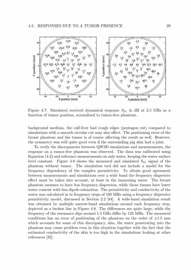
4.2. RESPONSES DUE TO A TUMOR PRESENCE 29
Figure 4.7: Simulated received dynamical response S31 in dB at 2.5 GHz as afunction of tumor position, normalized to tumor-free phantom.
background medium, the calf-liver had rough edges (pentagon cut) compared tosimulations with a smooth circular cut may also affect. The positioning error of thebreast phantom and the tumor is of course affecting the result as well. However,the symmetry was still quite good even if the surrounding pig skin had a joint.
To verify the discrepancies between QW3D simulations and measurements, theresponse on a tumor-free phantom was observed. The data was calibrated usingEquation (4.2) and reference measurements on only water, keeping the water surfacelevel constant. Figure 4.8 shows the measured and simulated S31 signal of thephantom without tumor. The simulation tool did not include a model for thefrequency dependency of the complex permittivity. To obtain good agreementbetween measurements and simulations over a wide band the frequency dispersiveeffect must be taken into account, at least in the immersing water. The breastphantom assumes to have less frequency dispersion, while those tissues have lowerwater content with less dipole-relaxation. The permittivity and conductivity of thewater was calculated in in frequency steps of 100 MHz using a frequency dispersivepermittivity model, discussed in Section 2.2 [84]. A wide-band simulation resultwas obtained by multiple narrow-band simulations around each frequency step,depicted as a broken line in Figure 4.8. The differences are quite large, while thefrequency of the resonance dips around 1.5 GHz differ by 125 MHz. The measuredconditions has an error of positioning of the phantom on the order of ±1.5 mmwhich accounts for some of this discrepancy, also, the water penetrating into thephantom may cause problem even in this situation together with the fact that theestimated conductivity of the skin is too high in the simulations looking at otherreferences [32].

30 CHAPTER 4. DETECTION OF BREAST TUMORS
1 1,5 2 2,5 3Frequency [GHz]
-100
-90
-80
-70
-60
-50
-40
Mag
nitu
de
[dB]
S31 MeasurementS31 simulation
Figure 4.8: Measured and simulated signal, S31, using a tumor-free phantom inwater.
Even if some phantom mismatches, antenna model mismatches and complexpermittivity mismatches etc. affecting the comparison between measurement resultsand simulation result, this example gives information about expected responsesduring measurements of a breast phantom. This information may be useful in thedecision of background medium and geometrical aspects of the tomograph system.If the data have very low responses from the internal object no iterative non-linearinverse solver would find the inhomogeneity [18, 40, 20]. Moreover, a noise freesituation was assumed in the simulations, while the dynamics in the data acquisitionhad a noise floor of -115 dB. Another comment worth noting is that only fatty breasttissues was assumed in the fantom, including fibroglandular tissues the contrastbetween the surrounding water and the breast tissues will be lower [10, 12].

Chapter 5
Quantitative Imaging with aPlanar Camera
The planar 2.45 GHz microwave camera, developed at Departement de Recherchesen Electromagnetisme (DRE) at Supelec, France, was one of the first developedmicrowave imaging system during the 80s [25, 39, 96, 61]. This system has mainlybeen used to create real-time qualitative images of the equivalent currents insideobjects using a linear spectral algorithm, [25, 26, 39], but Ann Franchois made greatefforts to generate quantitative reconstruction of homogeneous objects [62]. At thistime it was noted that the planar geometry obtains limited results compared to acylindrical setup and the circular setup was considered as an optimal geometry for2D quantitative imaging [63, 64].
There are several reasons why the planar setup has limited performance com-pared to cylindrical setups. One, is that some diffraction information is lost whilemeasuring only behind the object, according to chapter 4. Secondly, and probablythe largest influence, is the lower SNR at the edges of the measuring line due to theattenuation along the longer distance between the object and the receiver elementson the edges of the measuring line. However, beside of those limitations the planarcamera offers a great package of rapid acquisition on 1024 elements on a verticalplane behind an object. By using all those data a 2D reconstruction, where onlyone line is used, may be extended to a quasi-3D reconstruction, by using all thedata of the vertical plane. Even the vectorial 3D properties may be reconstructed ifthe camera is extended to measure both the vertical and horizontal polarized field.In this configuration the planar camera will offer a efficient platform with rapidmeasurements for both 2D and 3D reconstructions. This together with many otherimprovements of the camera motivates a new investigation of the capabilities toquantitatively reconstruct inhomogeneous objects such as a breast with a tumor.
31

32 CHAPTER 5. QUANTITATIVE IMAGING WITH A PLANAR CAMERA
5.1 Experimental setup
The planar microwave camera operates at a frequency of 2.45 GHz able to pro-vide data acquisition in real-time. It consists of two large horn-antennas, one fortransmitting and one for receiving, depicted in Figure 5.1 (left). The transmittinghorn-antenna is designed to produce a vertical polarized field consistent with anincident plane wave model, while using a centralized object. Between the two horn-antennas a large rectangular water tank is placed immersing the object under test.During normal operation pure water is used as immersing liquid.
The measured field is provided by a synthetic retina, which is placed in frontof the collector aperture as shown in Figure 5.1 (right). It consists of 1024 smalldipole antennas in a 32x32 array, with a step size of 7.2 mm (half the wavelengthin water) between each element. The retina is measuring at 1024 points alongthe vertical yz-plane, considering the plane wave propagates along the x-axis, thisenables image reconstruction of the object’s characteristics in horizontal as well asvertical cross sections. At first the retina may seem like a receiving part, but in
Figure 5.1: The retina (left) located in front of the receiving horn-antenna of thecamera (right).
fact this is a low frequency transmitter disturbing the plane wave transmitted bythe horn-antenna using the Modulated Scattering Technique (MST) [61, 96]. Onlyone retina element is active at once modulated at 200 kHz, the scanning is donerapidly line by line starting in the upper left corner of the retina, (looking fromthe transmitter). Each dipole-antenna is fed by a switching diode. The diode willopen and close producing a short circuit and open-ending during the modulation.Known from antenna theories this will produce an 180◦ phase-shift in the disturbedwave. A specific antenna element is selected by choose column and line by settingsufficient voltage levels on the Cy and Cz busses, depicted in Figure 5.2, (left).The active dipole antenna is modulated by a square-pulsed 200 kHz generating areceived response with a frequency modulation shown in complex plane in Figure5.2, (right). The large response is the response from the undisturbed plane wave.When modulating one retina element the response will move and oscillate between

5.1. EXPERIMENTAL SETUP 33
the two big dots in the complex plane. Note, that the low frequency results ofthe both big dots are similar but 180◦ phase-shifted, according to the open-endingand short circuit modulation of the antenna element, oriented from the plane wavecarrier response. Now, one may note that the response of one retina element is adisturbance of the plane-wave response. This disturbance will both change phaseand amplitude level dependent of the field at retina element position. Hence, theissue for the receiver hardware is to extract this disturbance response from theplane-wave response. Then by scanning trough all the 1024 points in the retina thesyntectic retina function is obtained.
Figure 5.2: General function of the retina (left) the matrix element functionality,(right) the complex response at the receiver.
The initial idea of the planar 2.45 GHz camera was to provide one-view imagesin real-time of a dynamic phenomena or at least with very fast acquisition. Benefit-ing from the spectacular rise of the microcomputer’s power and modifications of theacquisition and control system the camera is able to perform real-time reconstruc-tion of the equivalent currents in cross sections, by using a spectral method [39].In this real-time mode the rate of qualitative acquisitions/reconstructions reaches25 images/s. However, if quantitative results is wanted the Born approximationmay be used, (by approximating the internal field in the object as the same as theincident field). This approximation fails in the reconstruction while the object isrelatively large or having a high contrast in complex permittivity [38]. Hence, themost situations of biological applications an iterative non-linear inverse scatteringapproach is needed.
To obtain acquisition for quantitative reconstruction using a nonlinear inversescattering algorithm, multi-view acquisition has to be applied by using a electronicstep engine as rotator on top of the system, depicted in Figure 5.3. Many im-provements have been made on the system for the quantitative reconstruction ofinhomogeneous objects. The object is now fixed in the lower part of the water tankfor higher stability, increase the repeatability and avoid position error between the

34 CHAPTER 5. QUANTITATIVE IMAGING WITH A PLANAR CAMERA
rotation axis and the retina. A SNR of 50 dB is obtained by using averaging in theacquisition, also, minor hardware updates have improved the system’s dynamics.The water temperature is regulated at 37◦C (temperature of the human body).This induces a triple effect: 1) it reduces drastically the effects of the incident fielddrifts, 2) it improves the SNR by reducing the losses in water and 3) it decreases themodel errors due to variation on the complex permittivity. At last, minor changesof the transmitting horn-antenna has improved the homogeneity of the incidencefield. Note, that for 2D reconstruction purpose, only one line of the retina is used,while the field is measured in 1024 points in each view a efficient 3D accusationmay be obtained.
Figure 5.3: The experimental setup for quantitative imaging using the planar cam-era, the rotator on top and the temperature regulator (blue box) on the left.
One big advantage with the planar camera is the already implemented spectralalgorithm using filtered-backpropagation process. Using the real-time imaging thefield properties inside the experimental setup and object may be verified beforetime consuming multi-view acquisition is started. While, the equivalent currentsare imaged in real-time the response due to an inhomogeneity inside the object caneasily be verified in real-time, discussed in Chapter 4. Figure 5.4 shows an example,in the left the one view measured scattered field at the 32x32 retina is depicted ina situation using a cylindrical Plexiglas phantom with 100 mm diameter filled withsaline water (ε′ = 74, ε′′ = 14) and a small tube, 20 mm in diameter, filled witha saline/propandiol solution (ε′ = 68, ε′′ = 23). In this case it is impossible toobserve the effect of the inhomogeneity. By using the real-time capability andimage the differential difference of the field during rotation, the inhomogeneity’seffect is easily determined. In Figure 5.4 (right) the differential field at the retinais shown, in amplitude, between two views using the cylindrical phantom duringmulti-view operation. Here, one easily can see that qualitative real-time imagingis very useful to validate the experimental setup, to investigate if inhomogeneities

5.2. QUANTITATIVE IMAGES OF INHOMOGENEOUS OBJECTS 35
inside the object gives noticeable responses in the measured scattered field. If not,the quantitative algorithm will not have sufficient information in the measureddata. Note, in Figure 5.4 it is clear that the data from the planar camera contains
Figure 5.4: Qualitative images if the field on the retina using the real-time algorithm(left). A differential image of the field at the retina during the rotation of the object
information on the vertical plane behind the object, utilization of the completedata of the retina is a straight forward if a quasi-3D imaging algorithm is used.The retina offers a rapid measurement of the 3D space, with a modification of thesystem obtaining measurements of both the vertical and horizontal polarized fielda fully 3D imaging system is possible.
5.2 Quantitative Images of Inhomogeneous Objects
In paper C the ability of the planar 2.45 GHz camera to produce quantitativeimages for breast tumor detection is investigated. The imaging performance isstudied through simulations, verifying the tomographic ability to reconstruct theinhomogeneity inside the breast with a high contrast between the breast tissues andthe surrounding water, using the phantom in Figure 5.5. An elliptical breast modelis considered, whose dimensions are 100 x 76 mm containing a 15 mm diametertumor inside, depicted in Figure 5.5. The object is discretizised with a cell size of2λ/7 using 27 x 21 cells. The complex permittivity values used in the phantomare given in Table 5.1. Note that they come from a good compromise betweenmeasured values on existing phantoms materials and those found in the literaturepresented in Section 2.2.
The performance of planar geometry was compared with two circular systems[10, 63] using the open configuration Newton-Kantorovich code, presented in Section
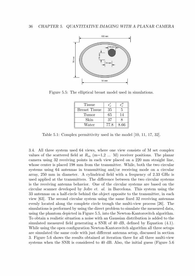
36 CHAPTER 5. QUANTITATIVE IMAGING WITH A PLANAR CAMERA
Figure 5.5: The elliptical breast model used in simulations.
Tissue ε′r ε′′rBreast Tissue 35 5
Tumor 65 14Skin 37 8
Water 77.8 8.66
Table 5.1: Complex permittivity used in the model [10, 11, 17, 32].
3.4. All three system used 64 views, where one view consists of M set complexvalues of the scattered field at Rm (m=1,2 ... M) receiver positions. The planarcamera using 32 receiving points in each view placed on a 220 mm straight line,whose center is placed 198 mm from the transmitter. While, both the two circularsystems using 64 antennas in transmitting and/or receiving mode on a circulararray, 250 mm in diameter. A cylindrical field with a frequency of 2.33 GHz isused applied at the transmitters. The difference between the two circular systemsis the receiving antenna behavior. One of the circular systems are based on thecircular scanner developed by Jofre et. al. in Barcelona. This system using the33 antennas on a half-circle behind the object opposite to the transmitter, in eachview [63]. The second circular system using the same fixed 32 receiving antennasevenly located along the complete circle trough the multi-view process [26]. Thesimulations is performed by using the direct problem to simulate the measured data,using the phantom depicted in Figure 5.5, into the Newton-Kantorovitch algorithm.To obtain a realistic situation a noise with an Gaussian distribution is added to thesimulated measured field generating a SNR of 40 dB, defined by Equation (4.1).While using the open configuration Newton-Kantorovitch algorithm all three setupsare simulated the same code with just different antenna setup, discussed in section3. Figure 5.6 shows the results obtained at iteration three for all three multi-viewsystems when the SNR is considered to 40 dB. Also, the initial guess (Figure 5.6

5.3. CALIBRATION 37
Figure 5.6: Complex permittivity distribution (up real part, down imaginary part),solution at iteration no3 with different multi-view systems for a SNR = 40 dB:(a) 2.45GHz planar camera (b) 2.33GHz Barcelona camera (c) 2.33 GHz completecircular system (d) initial guess (e) exact solution.
(d)) and the exact solution (Figure 5.6 (e)) are shown. From those results it appearsthat successful result may be obtained using the planar camera (Figure 5.6 (a)).The result are similar to the one obtained with the Barcelona system (Figure 5.6(b)) even if the Barcelona system using more input data, 2112 (64x33) instead of2048 (64x32) used in the other cases. The fixed complete circular system has a clearadvantage in the quality of reconstructed results, however this system has manypractical difficulties in a practical realization [26]. In paper C alternative usageof the camera in situations where antenna rotation is impossible for multi-viewacquisition. In this case a multi-incidence alternative, using fixed retina and objectwith an transmitter array, seems to be a potential alternative to obtain enoughindependent data for the reconstruction.
From those simulations it is clear that the planar 2.45 GHz camera definitelyis an interesting platform applied to the case of breast tumor detection. Using theplanar camera investigations about more specific 2D or 3D systems may be done.However, still, some work has to be focused on the experimental part to obtainquantitative images from experimental data.
5.3 Calibration
In quantitative microwave imaging using non-linear inverse scattering formalizationthe solution is determined by iteratively minimizing the error between the measuredfield and the computed field using a numerical model in the direct problem. Hence,it is of major importance that the numerical model in the direct problem and the

38 CHAPTER 5. QUANTITATIVE IMAGING WITH A PLANAR CAMERA
equipment are carefully calibrated. If not, the model error will make the recon-struction converge towards an nonphysical and wrong minimum, or if the modelerror is too large no convergence will be obtained at all. The calibration procedureof the planar 2.45 GHz camera may be divided into three principal parts.
• The transceiver calibration.
• Geometric and background medium properties of the equipment.
• The complex calibration vector of the equipment.
The first step, transceiver calibration is needed to suppress non-linearities anderrors introduced by the hardware. The received complex field are represented bythe I/Q–channels in the homodyne receiver, where the I–channel representing thereal part and the Q–channel representing the imaginary part with a 90o phase shiftin the complex plane. Therefore, it is important that both channels obtaining thesame gain and offset with a orthogonal behavior of the phase quadrature betweenthe channels. Franchois et. al. presented a method to calibrate those defects in[62, 98]. The idea is to perform calibration measurements by phase shift the inputsignal on the receiver between 0◦–360◦, in even steps, and then represent the I-and Q- channel results in the complex plane. A perfect system will in this caseobtain a circle with the center point in origo. However, the system defects willeventually produce results with an elliptical shape with the center on an offsetfrom origo. By estimating an elliptical model of the of the results and using a LeastMean Square (LMS) method for curve fitting of the data calibration coefficientscan be determined to produce a circular result. After several hardware updatesduring the preparation of this thesis an almost circular result was obtained withoutcalibration, making this calibration step unnecessary. However, still the calibrationbetween direct problem and equipment is necessary in the following steps.
The second step, concerns fitting of physical parameters in the experimentalsetup, such as the estimated complex permittivity of the surrounding water, thedistance rotation axis–retina R0 and the offset between the center-point of theretina with respect to the rotation axis Y0. Those parameters may of course bemeasured using different equipment like the Agilent Dielectric probe 85070E orusing the analytical water model developed by Stogryn et. al. [97]. Anothermethod, proposed in paper C, is to use the planar camera with an test-antennaas a source point. In this case the parameters are obtained by minimizing theerror between the field radiated by a source point and the one produced by aspherical wave model. The acquisition is done on a line of the retina when movinga short vertical monopole, which is supposed to radiate a spherical wave, along aline perpendicularly to the retina. The points using the same coordinates as therotation axis, therefore may the distance R0 be estimated.
The Final step, the complex coefficient to fit the measured field to the computedvalues in the direct problem. here two effective methods are developed by Meaney

5.3. CALIBRATION 39
et. al. and Jofre et. al. Meaney’s method is presented in Section 4.1, whicheffectively matching the measured field’s 3D properties to the 2D model. This isdone by taking the logarithmic difference between the the measured and computedfield without object, according to Equation (4.2). This calibration vector is thenused to correct the data from the acquisition with object. Jofre et. al. used a 40 mmmetallic reference cylinder and compared the measured values with the theoreticallyvalues. The correction vector for each emitter-receiver couple in the circular systemare found by dividing the theoretical measurement with the actual one. Using thecalibration vector on the measured data on the object gives a calibration of thewhole system [27, 63].
The method used herein may be seen as an combination of the other two group’s.When the first two steps are full filled the estimated parameters is used in the directproblem. The scattered field is computed in the direct problem using a referenceobject similar to Jofre et. al. A calibration vector is then computed from thedifferences of the computed and measured scattered field using the logarithmicamplitude and the phase like Meaney et. al. The correction vector’s amplitudeand phase is transformed to the complex plane. All data in multi-view experimentsare then multiplied with this vector. Both experimental and simulated data havebeen verified with analytical results, while good agreement is obtained betweenanalytical and simulated values simulations are used as reference. Note, only oneline is used during 2D image reconstruction.
As a reference object an 35 mm PVC cylinder is used, fixed at the rotationaxis. Also, the calibration vector may be defined by a global complex calibrationcoefficient defined from the center of the retina along line 15. Figure 5.7 showsan example of calibrated results using the global calibration coefficient. The phaseresults show a very good agreement, but the amplitude has larger errors especiallyon the outer skirt of the retina. However, as one can see a reasonable calibrationis obtained even with a perfect plane wave assumption in the simulations. Part ofthose defects may be solved by an calibration vector with individual calibration foreach specific retina element, but this could introduce large errors into the data whenthe differences are too large, e.g. along the outer skirt of the retina. However, themismatches in this area may be due to model mismatches between the plane wavemodel and the reality. This problem was observed by Franchois et. al. and theytried to include an experimental based model into the direct problem [98]. Thiswas not successful in experiments, but this could be a focus area at the moment,while the error in the incident field description has a major impact of the imagereconstruction [62].

40 CHAPTER 5. QUANTITATIVE IMAGING WITH A PLANAR CAMERA
Figure 5.7: Comparison between calculated and measured scattered field of a 35mm PVC cylinder with a complex correction of the measured field.

Chapter 6
Concluding Remarks
The work included in this Licentiate thesis was initiated during the establishmentof the microwave imaging research at the Department of Computer Science andElectronics at Malardalen University. Therefore, the work is initiated with feasi-bility studies together with a review of other group’s work. The later part of thiswork has been done in frame of a collaboration between Supeelec and MalardalenUniversity. Using the existing planar 2.45 GHz camera and the existing non-lineariterative Newton-Kantorovitch code, both developed at DRE of Supelec.
A state of the art review report has been created, covering the major contri-butions in both imaging systems and algorithms in the field of microwave imagingin biomedical applications, paper A. The focus has been on the area of breasttumor detection using microwave imaging. From the review it has been shown thatextended versions of the existing planar 2.45 GHz camera is an interesting platformfor investigating quantitative imaging of inhomogeneous objects as breast imaging.Earlier work showed that the planar 2.45 GHz camera is able to handle quantita-tive imaging of homogenous objects. One weak point with the planar setup is theshown limitation in reconstructed image quality for 2D imaging compared to a cir-cular configuration. The major advantage is, however, its high data acquisition rateon a vertical plane behind the object. The rapid 3D vertical polarization acquisitionis a big potential for quasi-3D imaging, or even fully vectorial 3D imaging with anextended version of the camera able to measure both the vertical- and horizontal-polarized field. Also, the single frequency 2D Newton-kantorovitch seems to be asolid starting point for future extension to the 3D problem of quantitative imagingfor breast tumor detection.
A feasibility study has been performed to indicate the expected response levelsdue to a tumor presence into a breast phantom, paper B. This knowledge is usefulat the moment of designing the tomographic acquisition system. Verifications maybe done in a early stage if the tumor inhomogeneity is detectable and in whichregions of the object are responses achieved. Also, the usefulness of an 3D FDTD
41

42 CHAPTER 6. CONCLUDING REMARKS
electromagnetic-wave simulator (QW3D) was verified.To verify the usefulness of the planar 2.45 GHz camera its tomographic per-
formance in a 2D reconstruction situation was compared with two other existingcircular systems paper C. This was possible though an extended open configura-tion Newton-kantorovitch code where the same algorithm effectively handle differentantenna configurations. It has been shown that the tomographic ability is similarcompared to the other two, breast image detecting a breast tumor has been obtainedin simulations with a SNR of 40 dB on the simulated measured scattered field. Fur-thermore, extensions leaving multi-view to multi-incidence system seems to be astrong alternative when a rotation is impossible in the acquisition. Good calibra-tion is achieved between experimental measurements and the algorithm. However,the amplitude is not fully satisfying and further efforts are needed before satisfyingexperimental quantitative results are obtained. A better estimation of the back-ground medium is needed in the calibration, also the differences between computedand measured field must be minimized. Those errors may be found in the modelerror due to the experimental incident field is not properly modeled with a perfectplane wave. In this case an incident field calibration has to be achieved to imple-ment an experimental based model of the incident field into the direct problem ofthe algorithm. At last, a realistic breast phantom modeling the breast tumor casehas to be designed.
6.1 Future Research
A major effort has been initiated in this work to establish a platform for quantitativeimaging of inhomogeneous using the planar 2.45 GHz camera at Supelec. Forthe moment the major focus is on obtaining 2D quantitative image reconstructionfrom experimental data of an inhomogeneous object using the Newton-Kantorovichalgorithm. Next step is to get result with a 2D breast phantom for the case of breasttumor detection. One necessary step may be to minimize the model error betweenthe algorithm and the experimental equipment. One way to minimize the modelerror is to implement an experimental based model of the incident field. Accordingto the conclusion of Franchois et. al. model error of the incident field error hasa major impact of the final result of the reconstruction. A possible method is touse the filtered-backpropagation process to compute the incident field in the objectregion of the Newton-Kantorovich code.
In the application of breast tumor detection there is in general two future di-rection. A multi-frequency approach similar to Meaney et. al. and Persson et.al. or 3D reconstruction. The big advantage of the planar camera is the rapidmeasurements on a plane behind the object, this setup could be used for inter-esting investigations of 3D imaging formalizations. However, the planar camera isa fixed frequency equipment optimized for 2.45 GHz, therefore, a multi-frequencyapproach needs a major hardware development. Therefore, the planar 2.45 GHz

6.1. FUTURE RESEARCH 43
camera is more suitable as a future platform for analyzing inhomogeneous objectsin 3D using both qualitative imaging in real-time and quantitative imaging withan iterative nonlinear algorithm. Using this system future breast tumor detectionspecific applications may be investigated.

44 CHAPTER 6. CONCLUDING REMARKS

Bibliography
[1] Sweden’s National Board of Health and Welfare: Causes of Death 2004,http://www.sos.se.
[2] D. M. Parkin, F. Bray, J. Ferlay and P. Pasaini, “Global Cancer Statics, 2002,”CA: Cancer Journal for Clinicians, vol. 55, pp. 74–108, Mar. 2005.
[3] J. S. Michaelson, M. Silverstein, J. Wyatt, G. Weber, R. Moore, E. Halbern,D. B. Kopans and K. Hughes, “Predicting the Survival of Patients with BreastCarcinoma using Tumor Size,” Cancer, vol. 95, pp. 713–723, Aug. 2002.
[4] C. H. Jones, “Methods of breast imaging, ” Phys . Med . Biol., vol. 27, 463-499,Apr. 1982.
[5] J. G. Elmore, D. L. Miglioretti, L. M. Reisch, M. B. Barton, W. Kreuter,C. L. Christiansen, S. W. Fletcher, “Screening Mammograms by CommunityRadiologists: Variability in False-Positive Rates,” J. Natl. Cancer Inst., vol. 94,pp. 1373–1380, Sep. 2002.
[6] P. T. Huynh, A. M. Jarolimek and S. Daye, “The False-Negative Mammogram,”Radiographics, vol. 18, pp. 1137–1154, 1998.
[7] M. Sabel and H. Aichinger, “Recent Developments in Breast Imaging,” Phys .Med . Biol., vol. 41, 315-368, Mar. 1996.
[8] V. P. Jackson, E. Hendrick, S. A. Feig, D. B. Kopans, “Imaging of the Radlo-graphically Dense Breast,” Radiology, vol. 188, pp. 287-301, 1993.
[9] M. Primic-Zakelj, “Screening Mammography for Early Detection of Breast Can-cer,” Ann. Oncol., vol. 10, pp. 121-127, 1999.
[10] P. M. Meaney, M. W. Fanning, D. Li, S. P. Poplack and K. D. Paulsen, “AClinical Prototype for Active Microwave Imaging of the Breast,” IEEE Trans.Microwave Theory Tech., vol. 48, pp. 1841–1853, Nov. 2000.
45

46 BIBLIOGRAPHY
[11] X. Li, S. K. Davis, S. C. Hagness, D. W. van der Weide and B. D. Van Veen,“Microwave Imaging via SpaceTime Beamforming: Experimental Investigationof Tumor Detection in Multilayer Breast Phantoms,” IEEE Trans. MicrowaveTheory Tech., vol. 52, pp. 1856–1865, Aug. 2004.
[12] A. Fhager, “ Microwave Tomography,” Ph.D. Thesis, Department of Signalsand Systems, Chalmers Univerity of Technology, 2006.
[13] G. Bindu, A. Lonappan, V. Thomas, C. K. Aanandan, and K. T. Mathew,Active Microwave Imaging for breast cancer detection,” Progress In Electro-magnetics Research PIER, vol. 58, pp. 149169, 2006.
[14] E. C. Fear, X. Li and S. C. Hagness, ”Confocal Microwave Imaging for BreastCancer Detection: Localization of Tumors in Three Dimensions,” IEEE Trans.Biomed. Eng., vol. 49, pp. 812–822, Aug. 2002.
[15] J. Bond, X. Li and S. C. Hagness, ”Microwave Imaging via Space-Time Beam-forming for Early Detection of Breast Cancer,” IEEE Trans. Antennas Propa-gat., vol. 51, pp. 1690–1705, Aug. 2003.
[16] E. C. Fear, P. M. Meaney and M. A. Stuchly, “Microwaves for Breast CancerDetection,” IEEE Potentials, pp. 12–18, Feb. 2003.
[17] D. Li, P. MMeaney and K. D. Paulsen, “Conformal Microwave Imaging forBreast Cancer Detection,” IEEE Trans. Microwave Theory Tech., vol. 51, pp.1179–1186, Apr. 2003.
[18] Q. Fang, P. M. Meaney, S. D. Geimer and A. V. Streltsov, “Microwave ImageReconstruction From 3-D Fields Coupled to 2-D Parameter Estimation,” IEEETrans. Medical Imag., vol. 23, pp. 475–484, Apr. 2004.
[19] N. Joachimowicz, C. Pichot and J. -P. Hugonin, “Inverse Scattering: An Iter-ative Numerical Method for Electromagnetic Imaging,” IEEE Trans. AntennasPropagat., vol. 39, pp. 1742–1752, Dec. 1991.
[20] N. Joachimowicz, J. J. Mallorqui, J. -C. Bolomey and A. Broquetas, “Conver-gence and Stability Assessment of Newton–Kantorovich Reconstruction Algo-rithms for Microwave Tomography,” IEEE Trans. Medical Imag., vol. 17, pp.562–570, Aug. 1998.
[21] W. C. Chew and Y. M. Wang,”Reconstruction of Two-Dimensional Permit-tivity Distribution Using the Distorted Born Iterative Method,” IEEE Trans.Medical Imag., vol. 9, pp. 218–225, Apr. 2004.
[22] J. H. Jacobi, L. E. Larsen and C. T. Hast, “Water-Immersed Microwave Anten-nas and Their Application to Microwave Interrogation of Biological Targets,”IEEE Trans. Microwave Theory Tech., vol. 27, pp. 70–78, Jan./ 1979.

BIBLIOGRAPHY 47
[23] L. E. Larsen and J. H. Jacobi, “Mcrowave Scattering Parameter Imaging odan Isolated Canine Kidney,” Medical Physics, vol. 6, pp. 394–403, 1979.
[24] A. Joisel, J. Mallorqui, A. Broquetas, J. M. Geffrin, N. Joachimowicz, M.V. Iossera, L. Jofre and J. -C. Bolomey, “Microwave Imaging Techniques forBiomedical Applications,” IEEE Instrumen. Measure. Tech. Conf., 1999.
[25] J. -C. Bolomey, L. Jofre and G. Peronnet “On the Possible Use of Microwave-Active Imaging for Remote Thermal Sensing,” IEEE Trans. Microwave TheoryTech., vol. 31, pp. 777–781, Sep. 1983.
[26] C. Rius, C. Pichot, L. Jofre, J. -C. Bolomey, N. Joachimowicz, A. Broque-tas and M. Ferrando, “Planar and Cylindrical Active Microwave TemperatureImaging: Numerical Simulations,” IEEE Trans. Medical Imag., vol. 11, pp.457–469, Dec. 1992.
[27] L. Jofre, M. S. Hawley, A. Broquetas, E. De Los Reyes, M. Ferrando and A. R.Elias-Fuste, “Medical Imaging with a Microwave Tomographic Scanner,” IEEETrans. Biomed. Eng., vol. 37, pp. 303–311, Mar. 1990.
[28] P. M. Meaney, K. D. Paulsen, A. Hartov and R. K. Crane, “An Actice Mi-crowave Imaging System for Reconstruction of 2-D Electrical Property Distri-butions,” IEEE Trans. Biomed. Eng., vol. 42, pp. 1017–1025, Oct. 1995.
[29] S. Y. Semenov, R. H. Svenson, A. E. Boulyshev, A. E. Souvorov, V. Y. Borisov,Y. Sizov, A. N. Starostin, K. R. Dezern, G. P. Tatsis and V. Y. Baranov,“Microwave Tomography: Two-Dimensional System for Biomedical Imaging,”IEEE Trans. Biomed. Eng., vol. 43, pp. 869–877, Sep. 1996.
[30] S. Y. Semenov, R. H. Svenson, A. E. Boulyshev, A. E. Souvorov, A. G.Nazarov, Y. E. Sizov, V. G. Posukh, A. Pavlovsky, P. N. Repin and G. P.Tatsis, “Spatial Resolution of Microwave Tomography for Detection of Myocar-dial Ischemia and InfarctionExperimental Study on Two-Dimensional Models,”IEEE Trans. Microwave Theory Tech., vol. 48, pp. 538–544, Apr. 2000.
[31] P. M. Meaney, Q. Fang, E. Demidenko and K. D. Paulsen, “Error Analysis inMicrowave Breast Imaging: Variance Stabilizing Transformations,” Procedingcof ICONIC 2005, UPC Barcelona, Spain, pp. 67–71, Jun. 2005.
[32] M. Miyakawa, T. Ishida and M. Watanabe,“Imaging Capability of an EarlyStage Breast Tumor by CP-MCT,” Procedingc of the 26th Annual InternationalConference of the IEEE EMBS San Francisco, CA, USA, Sep. 1-5, 2004.
[33] A. Fhager, P. Hashemzadeh, and M. Persson, “Reconstruction Quality andSpectral Content of an Electromagnetic Time-Domain Inversion Algorithm”,IEEE Trans. Biomed. Eng., vol. 53, pp. 1594–1604, Aug. 2006.

48 BIBLIOGRAPHY
[34] X. Li, E. J. Bond, B. D. van Veen and S. C. Hagness, “An Overview of Ultra-Wideband Microwave Imaging via Space-Time Beamforming for Early-StageBreast-Cancer Detection,” IEEE Antennas Propagat. Mag., vol. 47, pp. 19–34,Feb. 2005.
[35] J. -C. Bolomey, A. Izadnegahdar, L. Jofre, C. Pichot, G. Peronnet and M.Solaimani, “Microwave Diffraction Tomography for Biomedical Applications,”IEEE Trans. Microwave Theory Tech., vol. 30, pp. 1998–1982, Nov. 1982.
[36] C. Pichot, L. Jofre, G. Peronnet and J. -C. Bolomey, “Active Microwave Imag-ing of Inhomogeneous Bodies,” IEEE Trans. Antennas Propagat., vol. 33, pp.416–423, Apr. 1985.
[37] S. X. Pan and A. C. Kak, “A Computational Study of Reconstruction Algo-rithms for Diffraction Tomography: Interpolation Versus Filtered Backpropaga-tion,” IEEE Transactions on Acoustics, Speech and Signal Processing, vol. 31,pp. 1262–1275, Oct. 1983.
[38] M. Slaney, A. C. Kak, and L. E. Larsen, “Limitations of Imaging with First-Order Diffraction Tomography,” IEEE Trans. Microwave Theory Tech., vol. 32,pp. 860–874, Aug. 1984.
[39] A. Joisel and J. -C. Bolomey, “Rapid Microwave Imaging of Living Tissues,”SPIE Symp. Medical Imag. San Diego, CA, USA, Feb. 12-18, 2000.
[40] W. C. Chew and Y. M. Wang, “Reconstruction of two-dimensional permittivitydistribution using the distorted born iterative method,” IEEE Trans. MedicalImag., vol. 9, pp. 218–225, 1990.
[41] S. Caorosi, G. L. Gragnani and M. Pastorino, “Two-Dimensional MicrowaveImaging by a Numerical Inverse Scattering Solution,” IEEE Trans. MicrowaveTheory Tech., vol. 38, pp. 981–989, Aug. 1990.
[42] P. M. Meaney, K. D. Paulsen and T. P. Ryan, “Two-Dimensional HybridElement Image reconstruction for TM Illumination,” IEEE Trans. AntennasPropagat., vol. 43, pp. 239–247, 1995.
[43] K. D. Paulsen, P. M. Meaney, M. J. Moskowitz and J. M. Sullivan, “A DualMesh Scheme for Finite Element Based Reconstruction Algorithms,” IEEETrans. Medical Imag., vol. 14, pp. 504–514, Mar. 1995.
[44] P. M. Meaney, K. D. Paulsen, B. W. Pogue and M. I. Miga, “Microwave Im-age Reconstruction Utilizing Log-Magnitude and Unwrapped Phase to ImproveHigh-Contrast Object Recovery,” IEEE Trans. Medical Imag., vol. 20, pp. 104–116, Feb. 2001.

BIBLIOGRAPHY 49
[45] A. E. Souvorov, A. E. Bulyshev, S. Y. Semenov, R. H. Svenson, A. G. Nazarov,Y. E. Sizov, and G. P. Tatsis, “Microwave Tomography: A Two-DimensionalNewton Iterative Scheme,” IEEE Trans. Microwave Theory Tech., vol. 46, pp.1654–1659 , Nov. 1998.
[46] S. Caorsi, A. Massa, and M. Pastorino “A Numerical Solution to Full-Vector Electromagnetic Scattering by Three-Dimensional Nonlinear BoundedDielectrics,” IEEE Trans. Microwave Theory Tech., vol. 43, pp. 428–436 , Feb.2005.
[47] P. M. Meaney, Q. Fang, S. D. Geimer, A. V. Streltsov and K. D. Paulsen, “3DScalar Microwave Image Reconstruction Algorithm,” Microwave Symp. Digest,2002 IEEE MTT-S International, vol. 3, pp. 2269–2272, 2-7 June 2002.
[48] A. E. Bulyshev, A. E. Souvorov, S. Y. Semenov, V. G. Posukh and Y. E. Sizov,“Three-dimensional vector microwave tomography: theory and computationalexperiments,” Inverse Problems, vol. 20, pp. 1239-1259, 2004.
[49] A. Abubakar, P. M. van den Berg and S. Y. Semenov, “Two- and Three-Dimensional Algorithms for Microwave Imaging and Inverse Scattering,” Jour-nal of Electromag. Waves and Applicat., vol. 17, pp. 209–231, 2003.
[50] O. Franza, N. Joachimowicz and J. -C. Bolomey, “SICS: A Sencor Interac-tion Compensation Scheme for Microwave Imaging,” IEEE Trans. AntennasPropagat., vol. 50, pp. 211–216, Feb. 2002.
[51] K. D. Paulsen, P. M. Meaney, “Nonactive Antenna Compensation for Fixed-Array Microwave Imaging–Part I: Model Development”, IEEE Trans. MedicalImag., vol. 18, pp. 496–507, June 1999.
[52] P. M. Meaney, K. D. Paulsen, J. T. Chang, M. W. Fanning, and A. Hartov,“Nonactive Antenna Compensation for Fixed-Array Microwave Imaging PartII:–Imaging Results”, IEEE Trans. Medical Imag., vol. 18, pp. 508–518, June1999.
[53] A. Franchois and A. G. Tijhuis, “A Newton-Type Reconstruction Algorithm fora 434 Mhz Microwave Imaging Scanner,” Procedingc of the 22th URSI GeneralAsambly 2002, Maastricht, The Netherlands, 17-24 Aug. 2002.
[54] A. Abubakar, P. M. van den Berg and J. J. Mallorqui, “Imaging of BiomedicalData Using a Multiplicative Regularized Contrast Source Inversion Method,”IEEE Trans. Microwave Theory Tech., vol. 50, pp. 1761–1771, July 2002.
[55] S. Y. Semenov, A. E. Bulyshev, A. Abubakar, V. G. Posukh, Y. E. Sizov,A. E. Souvorov, P. M. van den Berg, and T. C. Williams, “Microwave-Tomographic Imaging of the High Dielectric-Contrast Objects Using Different

50 BIBLIOGRAPHY
Image-Reconstruction Approaches,” IEEE Trans. Microwave Theory and Tech.,vol. 53, pp. 2284–2294 , July 2005.
[56] S. Caorsi and P. Gamba, “Electromagnetic Detection of Dielectric Cylindersby a Neural Network Approach,” IEEE Trans. Geoscience Remote Sens., vol.37, pp. 820–827, Mar. 1999.
[57] M. Pastorino, A. Massa, and S. Caorsi, “A Microwave Inverse Scattering Tech-nique for Image Reconstruction Based on a Genetic Algorithm,” IEEE Trans.Instrumen. Measure., vol. 49, pp. 573–578, June 2000.
[58] M. Pastorino, S. Caorsi, A. Massa, and A. Randazzo, “Reconstruction Algo-rithms for Electromagnetic Imaging,” IEEE Trans. Instrumen. Measure., vol.53, pp. 692–699, June 2004.
[59] M. Pastorino, S. Caorsi, and A. Massa, “A Global Optimization Technique forMicrowave Nondestructive Evaluation,” IEEE Trans. Instrumen. Measure., vol.51, pp. 666–673, Aug. 2002.
[60] Q. Fang, P. M. Meaney, and K. D. Paulsen, “Microwave Image Reconstructionof Tissue Property Dispersion Characteristics Utilizing Multiple-Frequency In-formation,” IEEE Trans. Microwave Theory and Tech., vol. 52, pp. 1866–1875,Aug. 2004.
[61] Bolomey J. C. Gardiol Fred E. “Engineering Applications of the ModulatedScatterer Technique”, [Series: Artech House Antennar and Propagation Li-brary], ISBN: 1580531474.
[62] A. Franchois, A. Joisel, C. Pichot and J. -C. Bolomey, “Quantitative MicrowaveImaging with a 2.45-GHz Planar Microwave Camera,” IEEE Trans. MedicalImag., vol. 17, pp. 550–561, Aug. 1998.
[63] A. Broquetas, J. Romeu, J. M. Rius, A. R. Elias-Fuste, A. Cardama and L.Jofre, “Cylindrical Geometry: A Further Step in Active Microwave Tomogra-phy,” IEEE Trans. Microwave Theory Tech., vol. 39, pp. 836–844, May 1991.
[64] A. Franchois, C. Pichot”Microwave Imaging–Complex Permittivity Recon-struction with a Levenberg-Marquardt Method,” IEEE Trans. Antennas Prop-agat., vol. 45, pp. 203–215, Feb. 1997.
[65] P. M. Meaney, K. D. Paulsen and J. T. Chang, “Near-Field Microwave Imagingof Biologically-Based Materials Using a Monopole Trenceiver System,” IEEETrans. Microwave Theory Tech., vol. 46, pp. 31–43, Jan. 1998.
[66] J. M. Geffrin and A. Joisel, “Comparison of Measured and Simulated Inci-dent and Scattered Fields in a 434 Mhz Scanner,” Procedingc of the 22th URSIGeneral Asambly 2002, Maastricht, The Netherlands, 17-24 Aug. 2002.
BIBLIOGRAPHY 51
[67] S. Y. Semenov, R. H. Svenson, A. E. Boulyshev, A. E. Souvorov, A. G.Nazarov, Y. E. Sizov, A. Pavlovsky, V. Y. Borisov, B. A. Voinov, G. I. Si-monova, A. N. Starostin, V. G. Posukh, M. Taran, G. P. Tatsis, and V. Y.Baranov, “Three-Dimensional Microwave Tomography: Experimental Proto-type of the System and Vector Born Reconstruction Method,” IEEE Trans.Biomed. Eng., vol. 46, pp. 937–946, Aug. 1999.
[68] S. Y. Semenov, R. H. Svenson, A. E. Boulyshev, A. E. Souvorov, V. Y.Borisov, A. G. Nazarov, Y. E. Sizov, V. G. Posukh, A. Pavlovsky, P. N. Repin,A. N. Starostin, B. A. Voinov, M. Taran, G. P. Tatsis, and V. Y. Baranov,“Three-Dimensional Microwave Tomography: Initial Experimental Imaging ofAnimals,” IEEE Trans. Biomed. Eng., vol. 49, pp. 55–63, Jan. 2002.
[69] S. Y. Semenov, A. E. Boulyshev, A. E. Souvorov, A. G. Nazarov, Y. E. Sizov,R. H. Svenson, V. G. Posukh, A. Pavlovsky, P. N. Repin and G. P. Tatsis,“Three-Dimensional Microwave Tomography: Experimental Imaging of Phan-toms and Biologocal Objects,” IEEE Trans. Microwave Theory Tech., vol. 48,pp. 1071–1074, June 2000.
[70] M. Bertero, M. Miyakawa, P. Boccacci, F. Conte, K. Orikasa and M. Furutani,“Three-Dimensional Microwave Tomography: Initial Experimental Imaging ofAnimals,” IEEE Trans. Biomed. Eng., vol. 47, pp. 690–699, May 2000.
[71] P. M. Meaney, K. D. Paulsen, S. D. Geimer, S. A. Haider and M. W. Fanning,“Quantification of 3-D Field Effects During 2-D Microwave Imaging,” IEEETrans. Biomed. Eng., vol. 49, pp. 708–720, July 2002.
[72] N. Joachimowicz, “ Tomographie Microonde: Contribution a la Reconstruc-tion Quantitative Bidimensionnelle et tridimensionnelle,” PhD thesis, Univer-site Paris VII, Mars 1990.
[73] J. Bond, X. Li and S. C. Hagness, “Numerical and Experimental Investigationof an Ultrawideband Ridged Pyramidal Horn AntennaWith Curved LaunchingPlane for Pulse Radiation,” IEEE Antennas and Wireless Propagat. Letters,vol. 2, pp. 259–262, 2003.
[74] S. K. Davis, H. Tandradinata, S. C. Hagness, and B. D. Van Veen, “Ultraw-ideband Microwave Breast Cancer Detection: A Detection-Theoretic ApproachUsing the Generalized Likelihood Ratio Test,” IEEE Trans. Biomed. Eng., vol.52, pp. 1237–1250, July 2005.
[75] K. L. Carr, “Microwave radiometry: Its importance to the detection of cancer,”IEEE Trans. Microwave Tech., vol. 37, pp. 1862–1896, Dec. 1989.
[76] M. Miyakawa and T. Hayashi, “An Atemt of High-Speed Imaging of the ChirpRadar-Type Microwave Computed Tomography,” Microwave Symposium DigestIEEE MTT-S International, vol. 1, pp. 115–118, June 8-13, 1997.

52 BIBLIOGRAPHY
[77] M. Miyakawa, E. Harada and W. Jing, “Chirip Pulse Microwave ComputedTomography(CP-MCT) Equipped with a Fan Beam Scanner for High-speedImaging of a Biological Target,” Proceedings of the 25 Annual lntemationalConference of the IEEE EMBS, Caneun, Mexico, Sep. 17-21, 2003.
[78] M. Miyakawa, K. Orikasa, M. Bertero, P. Boccacci, F. Conte and M. Piana,“Experimental Validation of a Linear Model for Data Reduction in Chirp-PulseMicrowave CT,” IEEE Trans. Medical Imag., vol. 21, pp. 385–395, Apr. 2002.
[79] A. Fhager, M. Persson, “Comparisson of two image reconstruction algo-rithms for microwave tomography,” RADIO SCIENCE, vol. 40, RS3017,doi:10.1029/2004RS003105, 2005.
[80] K. R. Foster and H. P. Schwan, “Dielectric properties of tissues and biologicalmaterials: A critical review,” Crit. Rev. Biomed. Eng., vol. 17, pp. 25–104,1989.
[81] C. Gabriel, S. Gabriel, and E. Corthout, “The dielectric properties of biologicaltissues: I. Literature survey,” Phys. Med. Biol., vol. 41, pp. 2231–2249, 1996.
[82] S. Gabriel, R. W. Lau, and C. Gabriel, “The dielectric properties of biologicaltissues: II. Measurements on the frequency range 10 Hz to 20 GHz,” Phys. Med.Biol., vol. 41, pp. 2251–2269, 1996.
[83] S. Gabriel, R. W. Lau, and C. Gabriel, “The dielectric properties of biologicaltissues: III. Parametric models for the dielectric spectrum of tissues,” Phys.Med. Biol., vol. 41, pp. 2271–2293, 1996.
[84] R. Buchner, J. Barthel, and J. Stauber, “The dielectric relaxation of waterbetween 0◦ c and 35◦ c,” Chem. Phys. Lett., vol. 306, pp. 57–63, 1999.
[85] S. S. Chaudhary, R. K. Mishra, A. Swarup, and J. M. Thomas, “Dielectricproperties of normal and malignant human breast tissues at radiowave andmicrowave frequencies,” Indian J. Biochem. Biophys., vol. 21, pp. 76–79, 1984.
[86] A. J. Surowiec, S. S. Stuchly, J. R. Barr, and A. Swarup, “Dielectric propertiesof breast carcinoma and the surrounding tissues,” IEEE Trans. Biomed. Eng.,vol. 35, pp. 257–263, Apr. 1988.
[87] A. M. Campbell and D. V. Land, “Dielectric properties of female human breasttissue measured in vitro at 3.2 GHz,” Phys. Med. Biol., vol. 37, pp. 193–210,1992.
[88] W. T. Joines, Y.Z. Dhenxing, and R.L. Jirtle, “The measured electrical prop-erties of normal and malignant human tissues from 50 to 900 MHz,” Med. Phys.,vol. 21, pp. 547–550, 1994.

BIBLIOGRAPHY 53
[89] M. V. K. Chari, S. J. Salon, ”Numerical Methods in Electromagnetism, ”Academic Press, ISBN: 0-12-615760-X, 2000.
[90] R. F. Harrington, “Time-Harmonic Electromagnetic Fields, ” IEEE Press,ISBN: 0-471-20806-X.
[91] W. C. Chew G. P. Otto, W. H. Weedon, J. H. Lin, Y. M. Wang and M.Moghaddam, “Nonlinear Diffraction Tomography—The Use of Inverse Scatter-ing for Imaging,” Conference Record of The Twenty-Seventh Asilomar Conf.Signals, Systems and Computers, 1993., Vol. 1, pp. 120–129, 1-3 Nov. 1993.
[92] A. Roger, “Newton - Kantorovich algorithm applied to an electromagneticinverse problem,” IEEE Trans. Antennas Propagat., vol. 29, pp. 232-238, 1981.
[93] M. T. Heath, ”Scientific Computing, ” Second Edition, Mc Graw Hill, ISBN:0-07-112229-X, 2002.
[94] J. J. Mallorqui, N. Joachimowicz, A. Brouquetas, and J. C. Bolomey, “Quan-titative images of large biological bodies in microwave tomography by usingnumerical and real data,” IEE Electronics letters, vol. 32, pp. 2138–2140, 1996.
[95] M. Celuch-Marcysiak and W. K. Gwarek, “On the nature of solutions pro-duced by finite difference schemes in time domain,” Int. Journal of NumericalModelling, vol. 12, pp. 24–40, 1999.
[96] J. Ch. Bolomey, “Modulated probe arrays for rapid antenna testing; principleand applications,” Electronics/communications HF, vol. 2, pp. 35-46, 1997.
[97] A. Stogryn,“Equations for calculating the dielectric constant of saline water,”IEEE Trans. Microwave Theory Tech., vol. MTT–19, pp. 733-736, 1971.
[98] A.Franchois, “Contribution a la tomographie microonde: algorithmes de recon-struction quantitative et verifications experimentale,” PhD thesis, UniversiteParis-Sud Orsay, June 1993.

54 BIBLIOGRAPHY

Included Papers A-C
55