Microtremor measurements interpretations at the BVG station of the Italian accelerometric network 

 

Puglia R.1, Tokeshi K.2, Picozzi M.3, d’Alema E.4, Parolai S.3, Foti S.2 

1. Istituto Nazionale di Geofisica e Vulcanologia, Sezione di Milano‐Pavia, via Bassini 15, Milan, Italy  

2. Politecnico di Torino, corso Duca degli Abruzzi 24, Torino, Italy 

3. Helmholtz Centre Potsdam ‐ German Research Centre For Geosciences (GFZ), Helmholtzstraße 7, 14467 Potsdam, Germany 

4. Istituto Nazionale di Geofisica e Vulcanologia, Centro Nazionale Terremoti, strada Provinciale Cameranense snc, Passo Varano, Ancona, Italy 

 

Abstract 

In the last decades, researchers focused their attention on using inverse analysis of empirical surface‐waves dispersion curves from microtremor measurements since it allows to keep the cost of investigation relatively low and to avoid the use of active sources that might be prohibitive in urban areas.  

In this study we reports the results and interpretations of the passive measurements carried out at a test site in Bevagna (Italy) near the BVG station of the Italian Accelerometric Network (RAN) within the framework of the DPC‐INGV S4 Project (2007‐2009). Using two independent approaches, Rayleigh and Love wave dispersion characteristics were reproduced through two different inversion methods. At this site a cross‐hole test made nearby the seismic station offers the opportunity to compare the subsoil velocity profiles derived by seismic noise array data with independent geophysical information.  

The results obtained from the separated Love waves and Rayleigh wave inversions analyses showed that the two procedure provide consistent shear wave velocity profiles for the shallow part of the model in good agreement with the results of the nearby cross‐hole test.  

This case history shows the capabilities of surface wave analyses from passive source to adequately retrieve the S‐wave subsoil structure and suggests that more efforts should be devoted in exploiting the potential of coupled analysis of Rayleigh and Love waves from microtremor array measurements for site characterization. 

 

Introduction 

Surface wave analysis is often used for site investigation, specifically in order to get an estimate of the shear wave velocity profile. In particular the analysis of passive‐source data related to microtremors collected with 2D arrays have a good potential for characterization up to relevant depths avoiding the need for large and heavy sources. Most often the vertical components of microtremors are analysed referring to the propagation of Rayleigh waves. If a network of 3D geophones is used for the acquisition, also information on Love wave propagation can be used to get a shear wave velocity profile. Moreover a third information from surface wave propagation can be extracted from passive data. Indeed the H/V spectral ratio at each single station can provide very relevant information with respect to resonance frequencies of the soil deposit. This information can be used as a further constrain for surface wave dispersion inversion 

and also to check spatial variability of ground properties. The latter is a very relevant issue in surface wave analysis because the inversion is perfomed assuming a 1D soil model and checking this assumption is of paramount importance to evaluate the meaningfulness of the results. 

Microtremor measurements in array configuration were carried out by INGV‐Mi in September 2007 at a test site in Bevagna (Italy) nearby the BVG station (Figure 1) of the Italian accelerometric network (Rete Accelerometrica Nazionale, RAN). The BVG station was installed on a clayey formation (fluvial sediments in Figure 1b‐c) which may influence earthquake records in the frequency band of engineering interest.  

The purpose of this study is the one‐dimensional characterization of the clayey formation under the BVG station in terms of shear wave velocity (VS), i.e. the most representative parameter to estimate the subsoil seismic response, using two different approaches. In particular, observed Rayleigh and Love wave dispersion characteristics were reproduced through two different inversion methods. For brevity, hereafter these two approaches are simply recalled as Rayleigh and Love analyses. In both analyses Horizontal‐to‐Vertical Spectral Ratios of ambient vibrations (NHV) were used as a threshold for low frequencies, allowing to extend the depth of investigation.  

 

Figure 1 − Location of the Italian accelerometric network BVG station (a), geology settings of the study area (from the geological sheet of Italy n. 131 at scale 100.000, ISPRA) (b) and relative position between the BVG station and the array measurements (c). 

 

Experimental dataset 

Data were recorded for more than 3 hours using 15 Reftek 130 acquisition systems equipped with short‐period Lennartz LE‐3D/5s sensors and GPS timing. The sampling rate was fixed to 500 Hz, that is adequate for the frequency range and the inter‐station distance considered.  

The first common step of both the Rayleigh and Love measurements interpretations was the estimate of a single NHV spectral ratio representative for the whole array. The analysis of each station recordings in terms of NHV spectral ratio could be also useful to investigate the validity of the assumption of vertically 

(b) (c)

(a) 

heterogeneous 1D earth models, i.e. supposing significant lateral VS variations not affect the volume under the array measurement. In fact, both the Rayleigh and Love analyses here adopted, were employed under this assumption. 

In particular, smoothed NHV were calculated according to equation (1): 

  UP

WENSNHV22 +

=               (1) 

where, as usual, NS, WE and UP represent the Fourier spectra for each component of the recording. In this application, before the spectra computation, a baseline and an instrumental correction were applied to recordings and, then, a filter between 0.1 to 20 Hz. For each station, 50 signal windows of 200 seconds were expressed as Fourier spectra and smoothed and the relevant spectral ratio amplitudes – calculated by equation (1) – were considered log‐normally distributed to estimate the average curve. The smoothing operator here adopted is the Konno and Ohmachi (1998) with b=40. 

A predominant frequency of 1.0 Hz appear at all stations (Figure 2), except for BE01, BE09 and BE13, which, however, don’t present significant differences. Being these stations on the external boundary of the array, their different frequency response could be associated to lateral variations and/or close noise sources. Therefore, the assumption of vertically heterogeneous 1D VS model in the investigated volume of soil seems to be well satisfied.  

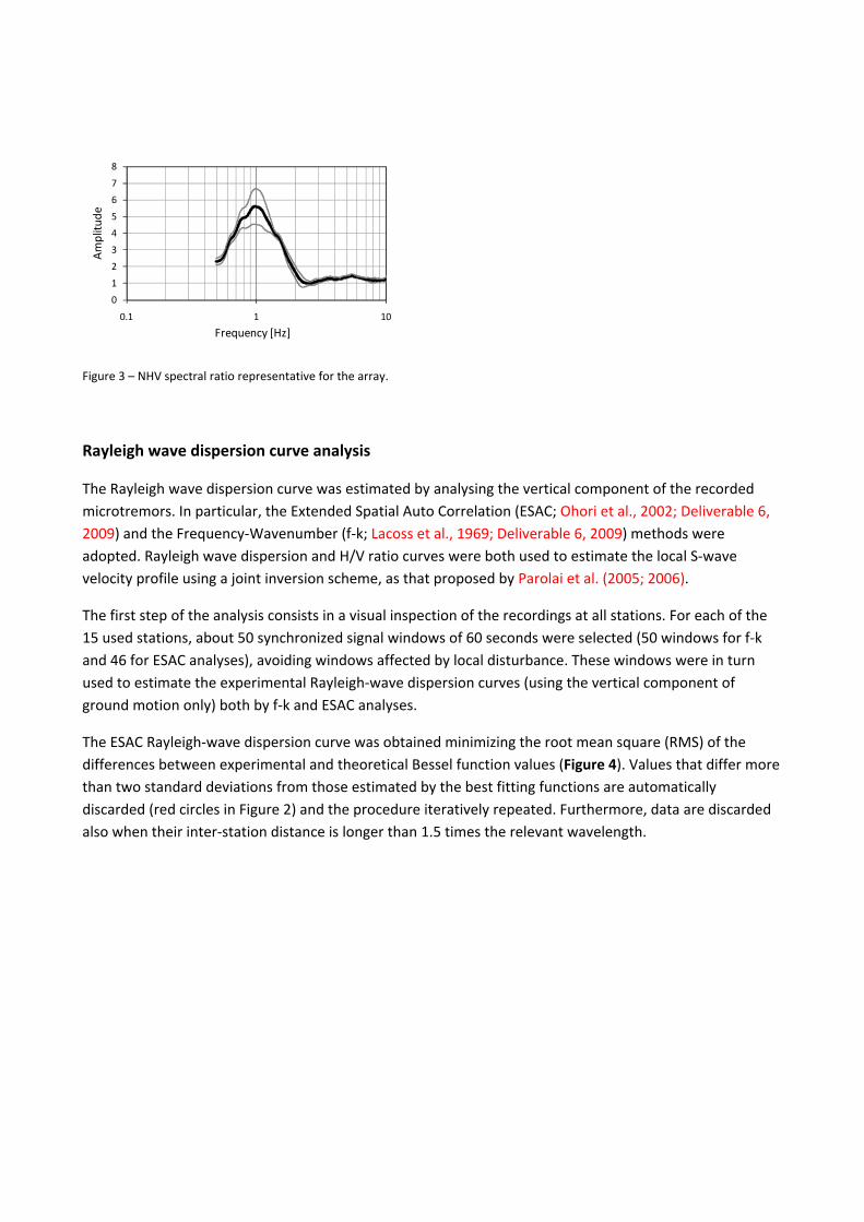
The average NHV curves for each station (Figure 2) were in turn averaged to obtain the input in the joint inversion procedures for the estimation of the S‐wave velocity profile (Figure 3). Microtremors recorded at BE01, BE09 and BE13 stations were not considered to construct the mean NHV. Although LE‐3D/5s sensors can reproduce frequencies in the range 0.2÷40 Hz, the minimum reliable frequency here considered is 0.5 Hz, since the trend of NHV ratios at lower frequencies clear shows problems due to installation (cf. recordings BE02, BE05, BE06, BE08, BE11, BE12 and BE15 in Figure 2).  

 

 

Figure 2 – NHV of the array microtremor measurements. 

 

0

1

2

3

4

5

6

7

8

0.1 1 10

Amplitu

de

Frequency [Hz] 

Figure 3 – NHV spectral ratio representative for the array. 

 

Rayleigh wave dispersion curve analysis 

The Rayleigh wave dispersion curve was estimated by analysing the vertical component of the recorded microtremors. In particular, the Extended Spatial Auto Correlation (ESAC; Ohori et al., 2002; Deliverable 6, 2009) and the Frequency‐Wavenumber (f‐k; Lacoss et al., 1969; Deliverable 6, 2009) methods were adopted. Rayleigh wave dispersion and H/V ratio curves were both used to estimate the local S‐wave velocity profile using a joint inversion scheme, as that proposed by Parolai et al. (2005; 2006).  

The first step of the analysis consists in a visual inspection of the recordings at all stations. For each of the 15 used stations, about 50 synchronized signal windows of 60 seconds were selected (50 windows for f‐k and 46 for ESAC analyses), avoiding windows affected by local disturbance. These windows were in turn used to estimate the experimental Rayleigh‐wave dispersion curves (using the vertical component of ground motion only) both by f‐k and ESAC analyses. 

The ESAC Rayleigh‐wave dispersion curve was obtained minimizing the root mean square (RMS) of the differences between experimental and theoretical Bessel function values (Figure 4). Values that differ more than two standard deviations from those estimated by the best fitting functions are automatically discarded (red circles in Figure 2) and the procedure iteratively repeated. Furthermore, data are discarded also when their inter‐station distance is longer than 1.5 times the relevant wavelength. 

 

 

Figure 4 – Experimental space‐correlation function values versus distance (circles) for different frequencies. The red circles indicate values discarded. The black lines depict the estimated space‐correlation function values for the phase velocity that furnishes the best fit to the data. The bottom panels show the relevant root‐mean square errors (RMS) versus phase velocity tested. 

 

Figure 5 shows the good agreement between the Rayleigh wave dispersion curves estimated both with ESAC and f‐k approaches (Maximum Likelihood Method). Only below 2.5 Hz the f‐k analysis provide larger phase velocities. The disagreement toward the lower frequencies confirms the results of previous studies (Parolai et al., 2007). Furthermore, problems arise with the ESAC method in estimating the phase velocity at around 3 Hz due to a strong persistent and directional source of noise. 

 

 

Figure 5 – Comparison of experimental phase velocity estimated by the ESAC and the f‐k (Maximum Likelihood Method) methods. The white squares represent the values used for the joint inversion. 

 

The f‐k analysis offers the opportunity to verify if the requirements on the noise source distribution for the application of the ESAC analysis were fulfilled and, overall, the reason of the previously observed poor coherency of the ESAC curve around 3 Hz. Figure 6 shows the output of the f‐k analysis at various frequencies.  

 

 

Figure 6 – f‐k power density function at different frequencies (a); map of the array measurement with the respective position of the “Statale dei Monti Martani” street and of an irrigation channel (b). 

North peak a)

b)

 

In Figure 6a contour plots at 2.5, 2.8 and 3.0 indicate the presence of noise propagating from two different directions. In particular, they evidenced that the highest energy is propagating from North (cf. map in Figure 6b) with a phase velocity of about 500 m/s. This phase velocity c0 is estimated for a certain frequency f0 applying equation (2): 

2yo

2xo

00

kk

f2πc+

⋅=                    (2) 

in correspondence of the f‐k power density functions peaks occurring at coordinates kxo and kyo (cf. contour maps in Figure 6 and the relevant values reported in Figure 7 with green circles and in Table 1). The high peaks with high velocity of propagation which appear on contour plots of f‐k power density function between 2.5 and 3 Hz may be probably due to human activities, but a clear location of the source was not yet possible. However, the activities existing in the nearby irrigation channel (evidenced by a blue colour in the map in Figure 6) could explain this source of noise. 

 

f0  kx0  ky0  c0 

0.0247  0.0166  527 2.5 

‐0.0439  0.0008  357 

0.0294  0.0193  501 2.8 

‐0.0499  0.0161  335 

0.0314  0.0193  511 3.0 

‐0.0541  0.0422  275 

0.0001  0.0954  211 ‐0.0656  0.0663  216 3.2 

‐0.1480  ‐0.0214  134 

‐0.0739  0.0777  205 ‐0.1605  ‐0.0422  132 0.0835  ‐0.1873  107 

3.5 

0.1200  ‐0.0798  153  

Figure 7 – Observed Rayleigh‐wave dispersion curves estimated by the f‐k method.  Green  circles  represent  the  phase  velocities  directly  obtained from f‐k power density functions peaks through Equation 2. 

Table 1 – Phase velocities directly obtained from f‐k power density functions peaks through Equation 2. 

 

Considering the observed reliability of the two methods (ESAC and f‐k) in estimating the phase velocity in different frequency bands for the data set at hand, we decided to combine the ESAC dispersion curve in the range 1.3÷2.5 Hz and 3.5÷5 Hz with the f‐k dispersion curve in the 2.5÷3.5 Hz range. The obtained dispersion curve is then used for the inversion (white squares in Figure 5). 

The non‐linear inversions were performed using a genetic algorithm (Yamanaka and Ishida, 1996) which does not rely upon an explicit starting model and allows the identification of a solution close to the global minimum. The forward modeling of Rayleigh wave phase velocities and H/V curves was performed using the modified Thomson‐Haskell method proposed by Wang (1999) and following the suggestions of Tokimatsu et al. (1992) and Arai and Tokimatsu (2004), under the assumption of vertically heterogeneous 1D earth models. The modeling of both the dispersion and NHV ratio curves during the inversions was not 

North peaks 

restricted to the fundamental mode only, but the possibility that higher modes can participate to define the observed dispersion and NHV curves is allowed.  

The inversion of dispersion and H/V curves to estimate the S‐wave velocity profile was carried out fixing to 5  the  number  of  layers  overlying  the  half‐space  in  the model  (Table  2).  Through  a  genetic  algorithm  a search over 80000 models was carried out. The inversion was repeated several times starting from different seed  numbers,  i.e.,  from  a  different  population  of  initial models.  In  this way  it was  possible  to  better explore the space of the solution.  

       

  Shear wave velocity, VS [m/s]  Thickness, h [m] 

Layer  MIN  MAX  MIN  MAX 

Density, ρ [ton/m3] 

#1  100  300  10  30  1.9 #2  200  600  20  80  1.9 #3  300  800  30  120  2.1 #4  400  900  30  120  2.2 #5  500  1200  50  400  2.2 Half‐space  600  2500  Infinite  2.3 

 

Table 2 – Parameters ranges used to joint inversion. 

 

During the inversion procedure the thickness and the shear wave velocity for each layer could be varied within the pre‐defined ranges. On the contrary, for each layer, density was assigned a priori, while compression wave velocity (VP) was calculated by equation (3), after defining the values of the shear wave velocity (VS). 

   1290 V1.1 [m/s] V SP +⋅=             (3) 

This empirical relationship was proposed and validated for deep soil deposits by Kitsunezaki et al. (1990). Poisson’s ratio was then obtained as a function of VS and VP.  

The models are selected on the basis of a cost function considering empirical and computed NHV and Rayleigh‐wave dispersion (c) curves (defined by equation (4), after Herrmann et al., 1999): 

( )[ ] ( ) ( )( )

( ) ( )( ) ⎪⎭

⎪⎬⎫

⎪⎩

⎪⎨⎧

⎥⎥⎦

⎤

⎢⎢⎣

⎡⎟⎟⎠

⎞⎜⎜⎝

⎛ −+

⎥⎥⎦

⎤

⎢⎢⎣

⎡⎟⎟⎠

⎞⎜⎜⎝

⎛ −−⋅+−= ∑∑

==

K

1j

2

O

ON

1j

2

O

O

fNHVfNHVfNHV

Kp

fcfcfc

Np1pKNp1cost  .   

(4) 

In the equation, the subscript “o” indicates observed data, whereas N and K are the number of data points in the dispersion and NHV curves, respectively. The relevant influence of both data sets is controlled by the parameter p. If p=0 the inversion is performed using only the apparent dispersion curve, while the inversion relies exclusively on the NHV for p=1. In this application, the weight p=0.04 was chosen after trial and error test.  

In Figure 8a tested models are depicted in different colours according to their relevant cost value: the more reliable model (minimum cost), the models lying inside the 10% range of the minimum cost, and the others tested models are shown in white, black and grey colours, respectively. The agreement between experimental and theoretical Rayleigh wave dispersion curves (gray and open circles in Figure 8c) is good and, considering the wavelengths related to the dispersion curve frequency range, the VS profile between 10 to about 150 metres is likely to be well constrained. Moreover, should be noticed that two families of profiles are predicted by the inversion procedure for the shallow part of the model (between 20 to 100m). However the differences are not so significant, in fact, both the families evidence the same trend: after the very well constrained share wave velocity contrast at a depth of 20m (from about 130 to 300‐340 m/s), the VS in the clay formation seems to have a gradually increasing until 450 m/s at 150m. 

 

Figure 8 – Shear wave velocity models at the BVG station (a): tested models (grey lines), the minimum cost model (white line), and models lying inside the minimum cost + 10% range (black lines). The generation values versus misfit (b). The fitting to the dispersion (c) and NHV ratio curves (d) in terms of experimental data (grey circles) and empirical values – relevant to the minimum cost model – (white circles). 

 

The deep part of the profile (over 150m of depth) and the impedance contrast between the clayey formation and the bedrock (between 500 and 600m of depth) are constrained using NHV only (Figure 8d). However, the profile from 150 down to 600m should be considered as a qualitative estimate, as also shown by the larger scattering of the profiles below 150m (Figure 8a).  

 

a)

d) 

c) 

b) 

Love wave dispersion curve analysis 

For estimating Rayleigh‐wave dispersion curve, 12 sets of 80 s vertical component records (BE2 – BE12) were considered simultaneously. The experimental Rayleigh‐wave dispersion curve (red squares in Figure 9) was estimated using the f‐k method (beam forming) through a software developed by the Natural Research Institute for Earth Science and Disaster Prevention of Japan. However, a narrow frequency band (1.5 – 2.1 Hz) was retrieved in the observed vertical Rayleigh‐wave dispersion curve. 

 

Figure 9 – Comparison of observed and theoretical Love‐wave / Rayleigh‐wave fundamental modes. 

 

Opposite to Rayleigh‐wave results, a clearer and larger frequency band (1.3 – 3.2 Hz) of experimental Love‐wave dispersion curve with lower standard deviation within the frequency band of 1.3 – 3.2 Hz was obtained from 12 sets of decomposed transversal f‐k spectra (red dots in Figure 9). The decomposed transversal horizontal components, which are supposed to contain predominantly Love‐waves, were obtained after rotating 20 deg the former horizontal components. The rotation of horizontal components was performed after observing similar predominant source directionalities in the f‐k spectra of vertical, transversal and radial components. The predominant directional angles of vertical dispersion curves, which horizontal dispersion curves showed a typical shape for dispersion curve, were detected coming predominantly from N20°E direction (in average). Figure 10 shows the predominant directional angle of the 3 components (vertical, transversal and radial components) obtained from one frame of 80 s, where predominant vertical directional angles of sources within 1.4 – 3.1 Hz are around 20 deg. Also, consistent predominant transversal directional angles of sources within 1.4 – 2.7 Hz were obtained around 20 deg, in average. Two examples of transversal f‐k spectra obtained for 2 and 2.7 Hz are shown in Fig. 11. 

The value of 1 Hz, which is the predominant NHV spectral ratio frequency in Fig. 3, was used as the threshold for extracting dispersion characteristics of Love waves.  

Bevagna

0

500

1000

0 1 2 3 4 5

Frequency (Hz)

Phase v

elo

city (m

/s)

7 best results

Obs. Rayleigh-wave dispersion

± 10% phase velocity

Obs. Love-wave dispersion

 740 

1.3 

 

Figure 10 – Predominant directional angle of sources versus frequency obtained from vertical, transversal and radial f‐k spectral analysis (80 s frame). 

 

 

Figure 11 – f‐k spectra obtained from transversal components of microtremor records. 

 

 

Estimation of soil profiles using random search 

For the inverse analysis, a ground model of a horizontally 4 layered soil overlying a half‐space was used (Table 3). A random search (Monte Carlo inversion) on three parameters (S‐wave velocity, thickness and Poisson’s ratio) for each layer was used. The two first parameters, the S‐wave velocity and the thickness, have strong influence on the Rayleigh‐ and Love‐wave phase velocities. The third significant parameter on dispersion curves is the density (Xia et al., 1999), which is calculated empirically with the P‐wave velocity (Gardner et al., 1974), and in turn, is correlated with the Poisson’s ratio and the S‐wave velocity (Tokeshi et al., 2008). 

-180

-90

0

90

180

1 2 3 4 5 6

Frequency ( Hz )

Azi

mut

h (

deg

)

Vertical

Transversal

Radial

  Average directional angle = 20 deg

Poisson’s ratio, ν  Shear wave velocity, VS [m/s]  Thickness, h [m] Layer 

MIN  MAX  MIN  MAX  MIN  MAX 

#1  400  30 

#2  700  100 

#3  1000  100 

#4 

0.25  0.49  100 

1500 

1 

100 

Half‐space  VP = 3800    VS = 2500  Infinite  

Table 3 – Ranges used in parameters for random inverse analysis. 

 

One million trials were performed during random search, and in order to improve the efficiency of the algorithm, the value of the SH‐wave resonance frequency of each ground model trial was calculated. Only the random models whose resonance frequencies were lower than the threshold frequency of 1 Hz proceeded to the next step. Then, the theoretical Love‐wave fundamental mode for each ground model was compared with the observed one, by checking how many points the phase velocity of Love‐wave fundamental mode is within the relative error of 10% observed phase velocity (black hyphen in Figure 9). After finishing the random search, the possible ground systems were lined up according to the number of points that satisfied the previous condition and the least‐square‐misfit criterion. 

Figure 9 shows the comparison between the observed and the theoretical Love fundamental dispersion curves of the 7 best solutions that satisfied the condition for 20 points (all frequencies). Also, the comparison between an observed Rayleigh dispersion curve obtained from one frame of 80 s and the theoretical Rayleigh fundamental modes associated to the 7 ground models is shown in Figure 9, with good agreement between both observed and theoretical Love / Rayleigh‐waves fundamental modes.  

 

Comparison of Rayleigh and Love waves analyses with other tests available in the study area 

The results obtained from the separated Rayleigh and Love waves inversions analyses showed that the two procedures provide consistent shear wave velocity profiles for the shallow part of the model (Figure 12). In particular, the seismic impedance contrast in the clay formation at about 20 m of depth and the shear wave velocity of about 150 m/s attributed to the first layer, which were estimated by both the inversion procedure here applied, is confirmed by the results of a nearby Cross‐Hole (CH) test carried out at BVG site in the framework of the DPC‐INGV S6 Project (Luzi and Sabetta, 2006). 

Below 20 m, the Rayleigh waves inversions analysis estimates a layer characterized by a VS of 340 m/s (300 m/s considering the less probable family). Although it underestimates the VS measured with the CH test at depth ranging from 20 to 30 m, the Rayleigh waves analysis is very well constrained by the dispersion curve below to about 50 m. In fact, the agreement between the experimental and estimated dispersion curves for frequencies higher than 2.5 Hz is excellent (Figure 8c). Probably the VS estimate by the Rayleigh waves analysis for this layer is an average of the subsoil shear wave velocities at depth between 20 to 50 m. Furthermore, although the Rayleigh waves analysis take into account higher modes, it was not able to reproduce the velocity inversion evidenced in the CH test at 30 m of depth, probably because of the layering ranges adopted in the inversion procedure (cf. Table 2). 

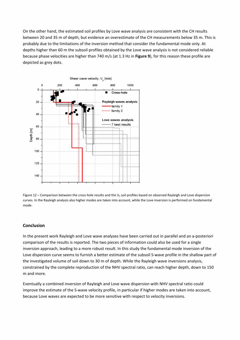
On the other hand, the estimated soil profiles by Love wave analysis are consistent with the CH results between 20 and 35 m of depth, but evidence an overestimate of the CH measurements below 35 m. This is probably due to the limitations of the inversion method that consider the fundamental mode only. At depths higher than 60 m the subsoil profiles obtained by the Love wave analysis is not considered reliable because phase velocities are higher than 740 m/s (at 1.3 Hz in Figure 9), for this reason these profile are depicted as grey dots. 

 

 

Figure 12 – Comparison between the cross‐hole results and the VS soil profiles based on observed Rayleigh and Love dispersion curves. In the Rayleigh analysis also higher modes are taken into account, while the Love inversion is performed on fundamental mode. 

 

Conclusion 

In the present work Rayleigh and Love wave analyses have been carried out in parallel and an a‐posteriori comparison of the results is reported. The two pieces of information could also be used for a single inversion approach, leading to a more robust result. In this study the fundamental mode inversion of the Love dispersion curve seems to furnish a better estimate of the subsoil S‐wave profile in the shallow part of the investigated volume of soil down to 30 m of depth. While the Rayleigh wave inversions analysis, constrained by the complete reproduction of the NHV spectral ratio, can reach higher depth, down to 150 m and more. 

Eventually a combined inversion of Rayleigh and Love wave dispersion with NHV spectral ratio could improve the estimate of the S‐wave velocity profile, in particular if higher modes are taken into account, because Love waves are expected to be more sensitive with respect to velocity inversions.  

 

Acknowledgments 

The work is part of the INGV‐DPC S4 Research Project “Italian Strong Motion Data Base”, promoted by the Istituto Nazionale di Geofisica e Vulcanologia (INGV) and funded by the Dipartimento della Protezione Civile (DPC) of the Italian Government (Agreement INGV‐DPC 2007‐2009). The authors wish to thank the DPC and the project team coordinators, Dr. Francesca Pacor and Prof. Roberto Paolucci, for their valuable scientific and administrative support. The INGV‐Mi team (composed of Dr. Dino Bindi, Ezio D’Alema, Sara Lovati and Dr. Marco Massa) which previously executed the in situ microtremor measurements is also warmly acknowledged. Likewise, thanks to the Regione Piemonte for financing Ken Tokeshi’s grant. 

 

References 

Arai H. and K. Tokimatsu, 2004. S‐wave velocity profiling by inversion of microtremor H/V spectrum, Bull. Seism. Soc. Am., 94, 53–63. 

Deliverable 6, 2009. Coordinators: Pacor F. and Paolucci R.; edited by: Foti S., Parolai S. and Albarello D.; contributors: Albarello D., Comina C., Foti S., Maraschini M., Parolai S., Picozzi M., Puglia R. and Tokeshi K.; Research Report of DPC‐INGV S4 Project 2007‐2009. http://esse4.mi.ingv.it 

Gardner G. H. F., Gardner L. W. and Gregory A. R., 1974. Formation velocity and density; the diagnostic basics for stratigraphic traps. Geophysics, 39, 770‐780. 

Herrmann R.B., Ammon C.J., Julia J. and Mokhtar T., 1999. Joint inversion of receiver functions and surface‐wave dispersion for crustal structure. Proc. 21st Seismic Research Symposium Technologies for monitoring the comprehensive Nuclear test Ban treaty, September 21‐24, 1999, Las Vegas, Nevada, USA, published by Los Alamos National Laboratory, LA‐UR‐99‐4700. 

Kitsunezaki C., Goto N., Kobayashi Y., Ikawa T., Horike M., Saito T., Kurota T., Yamane K. and Okozumi K., 1990. Estimation of P‐ and S‐wave velocities in deep soil deposits for evaluating ground vibrations in earthquake. J.JSNDS, 9, 1‐17. 

Konno K. and Ohmachi T., 1998. Ground‐Motion Characteristics Estimated from Spectral Ratio between Horizontal and Vertical Components of Microtremor, Bull. Seism. Soc. Am., 88, 228‐241. 

Lacoss R.T., Kelly E.J., Toksöz M.N., 1969. Estimation of seismic noise structure using arrays, Geophysics, 34, 21‐38. 

Luzi L. and Sabetta F., 2006. Data base dei dati accelerometrici italiani relativi al periodo 1972‐2004. DPC‐INGV S6 Project 2004‐2006. http://esse6.mi.ingv.it/ 

Ohori M., Nobata A., and Wakamatsu K., 2002. A comparison of ESAC and FK methods of estimating phase velocity using arbitrarily shaped microtremor analysis, Bull. Seism. Soc. Am., 92, 2323‐2332. 

Parolai S., Picozzi M., Richwalski S.M. and Milkereit C., 2005. Joint inversion of phase velocity dispersion and H/V ratio curves from seismic noise recordings using a genetic algorithm, considering higher modes, Geoph. Res. Lett., 32, doi: 10.1029/2004GL021115. 

Parolai S., Richwalski S.M., Milkereit C. and Faeh D., 2006. S‐wave velocity profile for earthquake engineering purposes for the Cologne area (Germany), Bull. Earthq. Eng., 65–94, doi:10.1007/s10518‐005‐5758‐2. 

Parolai S., Mucciarelli M., Gallipoli M.R., Richwalski S.M. and Strollo A., 2007. Comparison of Empirical and Numerical Site Responses at the Tito Test Site, Southern Italy, Bull. Seism. Soc. Am., 97, 1413‐1431. 

Tokeshi K., Karkee M. and Cuadra C., 2008. Estimation of Vs profile using its natural frequency and Rayleigh‐wave dispersion characteristics. Adv. Geosci., 14, 75‐77. www.adv‐geosci.net/14/75/2008/. 

Tokimatsu K., Tamura S. and Kojima H., 1992. Effects of multiple modes on Rayleigh wave dispersion characteristics. Journal of Geotechnical Engineering 118, 1529–1543. 

Wang R., 1999. A simple orthonormalization method for stable and efficient computation of Green’s functions. Bulletin of the Seismological Society of America 89, 733–741. 

Xia J., Miller R. D. and Park C. B., 1999. Estimation of near‐surface shear‐wave velocity by inversion of Rayleigh waves. Geophysics, 64, 691‐700. 

Yamanaka H. and Ishida H., 1996. Application of Generic algorithms to an inversion of surface‐wave dispersion data. Bull. Seism. Soc. Am. 86, 436‐444.