Microsimulation Framework to Explore Impact of Truck Platooning on Traffic Operation and Energy Consumption:

Development and Case Study

PATH Research Report for

FHWA Exploratory Advanced Research Program

Cooperative Agreement DTFH61-13-H00012

Tasks 1.4 and 2.7

Hani Ramezani, Steven E. Shladover, Xiao-Yun Lu, Fang-Chieh Chou

California PATH Program

Institute of Transportation Studies

University of California, Berkeley

February 2018

List of Tables ............................................................................................................................................... iii

List of Figures .............................................................................................................................................. iv

Abstract ......................................................................................................................................................... 1

Executive Summary ...................................................................................................................................... 2

Introduction ................................................................................................................................................... 4

Chapter 1 Effect of Truck Platooning on Traffic Operation ...................................................................... 6

1.1 Mechanism of Automatic Vehicle Following ............................................................................... 6

1.2 Car Following Models .................................................................................................................. 7

1.2.1 Manual mode car following models ...................................................................................... 8

1.2.2 Automated mode car following models ................................................................................ 8

1.2.3 Switch from an automated mode to manual mode ................................................................ 9

1.2.4 Desired speed computation ................................................................................................. 10

1.2.5 Lane changing models ........................................................................................................ 10

1.2.6 Lane change cooperation .................................................................................................... 10

1.3 Case Study: I-710 Northbound ................................................................................................... 11

1.3.1 Parameter selection ............................................................................................................. 12

1.3.2 Parameter calibration .......................................................................................................... 15

1.4 Results ......................................................................................................................................... 15

1.4.1 Corridor analyses ................................................................................................................ 16

1.4.2 Analyses at individual loop detector locations .................................................................... 16

1.4.3 Detailed analyses for selected loop detector stations .......................................................... 18

1.5 Conclusions ................................................................................................................................. 19

Chapter 2 Effect of Truck Platooning on Energy Consumption .............................................................. 22

2.1 MOVES Overview ...................................................................................................................... 22

2.1.1 Energy consumption for passenger cars .............................................................................. 22

2.1.2 Energy consumption for diesel trucks ................................................................................. 24

2.2 MOVES Modifications ............................................................................................................... 25

2.2.1 Quantization issue in MOVES ............................................................................................ 26

2.2.2 Energy consumption reduction factors for different operating modes ................................ 28

Step-by-step procedure to compute a reduction factor for a given operating mode ........................... 29

2.3 Case Study .................................................................................................................................. 30

2.3.1 Corridor level analysis ........................................................................................................ 31

2.3.2 Link level analysis .............................................................................................................. 33

i

2.4 Conclusions ................................................................................................................................. 35

Chapter 3 Development of Vehicle Following Models ........................................................................... 36

3.1 Experiment Description .............................................................................................................. 36

3.2 System Identification Modeling Method .................................................................................... 36

3.2.1 Cruise control driven truck ................................................................................................. 37

3.2.2 Adaptive cruise control driven truck ................................................................................... 41

3.2.3 Cooperative adaptive cruise control driven truck ............................................................... 44

3.3 Conclusions ................................................................................................................................. 46

References ................................................................................................................................................... 47

ii

List of Tables

Table 1-1: Maximum acceleration rates for trucks (25) ............................................................................. 13 Table 1-2: Calibrated values of car following parameters ......................................................................... 16 Table 2-1: Projecting experiment results for different gaps ....................................................................... 26 Table 2-2: Re-calibrated values for road load coefficient C ...................................................................... 28 Table 2-3: Platooning pattern in one simulation run .................................................................................. 33 Table 3-1: Summary of the parameter sets for CC model ......................................................................... 39 Table 3-2: CC model validation summary ................................................................................................. 40 Table 3-3: Summary of the parameters for ACC model ............................................................................ 42 Table 3-4: ACC model validation summary .............................................................................................. 42 Table 3-5: Summary of the parameter sets for CACC model .................................................................... 45 Table 3-6: CACC validation summary ...................................................................................................... 45

iii

List of Figures

Figure 1-1: Simulation logic to determine leaders and followers and their regulation modes ..................... 7 Figure 1-2: a) I-710 NB corridor and loop detector locations (red bars) b) Location of the most congested detector modeled in Aimsun ...................................................................................................................... 12 Figure 1-3: Comparison of simulation and field data at eleven detector stations for simulation using the calibrated parameter values ........................................................................................................................ 14 Figure 1-4: Effects of truck CACC at eleven detector stations for cars and trucks ................................... 17 Figure 1-5: Speed increase due to truck CACC versus base case speed plotted for eleven detector stations ................................................................................................................................................................... 18 Figure 1-6: Speed and flow rate variations over time for two loop detectors ............................................ 21 Figure 2-1: Determination of a) operating modes and b) energy consumption rates for passenger cars ... 23 Figure 2-2: Energy consumption rates for diesel trucks ............................................................................ 25 Figure 2-3: Energy (fuel) savings in a truck platooning experiment (retrieved from 11) .......................... 26 Figure 2-4: Energy consumption rates for diesel trucks interpolated and smoothed in speed Class 3 ...... 27 Figure 2-5: Projected energy savings for different operating modes ......................................................... 30 Figure 2-6: I-710 simulation results: estimated energy saving for different replications .......................... 32 Figure 2-7: Aerodynamic energy saving for links versus a) degree of AEP, and b) average truck speed . 33 Figure 2-8: Link analysis a) histogram of energy usage change b) energy usage change versus cumulative energy consumption ................................................................................................................................... 34 Figure 2-9: Effect of link speeds on energy consumption ......................................................................... 35 Figure 3-1:Block diagrams of automated vehicle following models ......................................................... 39 Figure 3-2: Field test data compared to estimates based on P-model and PI-model for CC mode. ........... 41 Figure 3-3: Field test data compared to model predictions for ACC mode ............................................... 43 Figure 3-4: Field test data compared to model predictions for CACC mode ............................................ 46

iv

Abstract Cooperative adaptive cruise control (CACC) systems have the potential to improve traffic flow and energy consumption efficiency, but these effects are challenging to estimate. This report presents the development of a micro-simulation model to represent these impacts for heavy trucks using CACC when they share a freeway with manually driven passenger cars. The simulation incorporates automated truck following models which have been derived from experimental data recorded on heavy trucks driven under CACC, adaptive cruise control (ACC), and conventional cruise control (CC). The simulation includes other behavioral models for lane changing, lane change cooperation and lane use restrictions for trucks to better capture real-world traffic dynamics. The developed simulation model was used to conduct a case study for a 15-mile urban freeway corridor with heavy truck traffic and significant congestion. Effects of truck CACC on traffic operation and energy consumption were studied. Simulation results show that truck CACC improved traffic operations for trucks in terms of Vehicle Miles Traveled (VMT), average speed and flow rate. In addition, truck CACC did not adversely affect passenger car operations and in some locations it even produced considerable improvements in the general traffic conditions.

A procedure was developed based on the Motor Vehicle Emission Simulator (MOVES) to estimate energy savings for in-platoon trucks. MOVES was re-calibrated using experimental data; and the calibrated MOVES was used to estimate energy saving rates for conditions that have not been covered in the experimental data, but that may occur in a simulation. The procedure was integrated with the microsimulation to study the same 15-mile urban freeway corridor. Results showed that energy consumption per VMT decreased for trucks. The energy consumption decrease originates only partially from aerodynamic drag reduction but primarily from congestion reduction due to platooning.

1

Executive Summary A very basic form of automated speed control is Cruise Control (CC) which has been widely available for many years. In CC, a vehicle travels with a constant speed that is determined by the driver. An improved version of the automated speed control is Adaptive Cruise Control (ACC) that regulates speed of a vehicle based on its gap and speed relative to the lead vehicle. Cooperative Adaptive Cruise Control (CACC) augments the automatic vehicle following capabilities of ACC with the addition of vehicle-to-vehicle (V2V) wireless communication of data about the movements of nearby vehicles; as a result, vehicles can more quickly and effectively adjust their speed and gap with respect to lead vehicles. CACC systems have the potential to improve traffic flow and energy consumption efficiency, but these effects are challenging to estimate. This report presents development of a microsimulation model and implements the model on a 15-mile congested urban freeway corridor to estimate these effects.

A micro simulation model was developed to study automated trucks and manually driven cars on an urban highway. One of the contributions of the study is to develop vehicle dynamic models for these truck automation modes: 1) CACC, 2) ACC, and 3) CC. The data representing these automation modes come from tests of a 3-truck platoon which was traveling mixed with manually driven vehicles on an urban highway. To the best of the authors’ knowledge, there were no such vehicle dynamics models for heavy trucks available in the literature.

In addition, the simulation model incorporates several models for driver usage of partially automated trucks to add more sophistication and reliability in analysis. Examples of these models are: 1) Mandatory and discretionary lane changing, 2) Lane change cooperation, 3) Lane use restrictions for trucks (i.e. avoid faster lanes) 4) Circumstances to switch among three automation modes, and 5) Conditions for driver to turn off automation and take over the truck to avoid collisions.

To estimate the effects of truck CACC on traffic operations, a case study was conducted for a 15-mile urban freeway corridor which experienced both congested and uncongested conditions during a one-hour simulation period. Results of five simulation replications showed that 100% truck usage of CACC improved traffic operations for trucks and cars at different locations. In particular, truck CACC could postpone the onset of congestion, and it could increase traffic speed at some uncongested locations. Corridor level analysis for trucks demonstrated that average speed increased from 33.3 mph to 39.7 mph, and Vehicle Miles Traveled (VMT) increased by 5.8%. The results also showed that truck CACC did not adversely affect traffic operations for cars, and at some locations it even brought a significant speed increase. Corridor level analysis for cars showed that their average speed increased from 49.3 mph to 52.4 mph, and VMT increased by 0.7%.

2

A procedure was developed based on the Motor Vehicle Emission Simulator (MOVES) to estimate energy consumption when trucks are driven in a platoon. MOVES is a computer program widely used within EPA to estimate energy consumption and emission rates for mobile sources. MOVES does not consider effect of truck platooning on aerodynamic drag reduction. To resolve this issue, the MOVES model was re-calibrated to replicate the energy savings measured in a CACC experiment. Then, energy saving rates were computed for conditions which have not been covered in an experiment, but that can happen in a simulation study. To estimate the effects of truck CACC on energy consumption, the developed procedure was integrated with the microsimulation model, and it was implemented on the same 15-mile corridor. Results showed that energy consumption per VMT was reduced for trucks by an average of 3.05%. This reduction comes from two sources:

1) Aerodynamic drag reduction, which is associated with 0.48% energy saving, and 2) Congestion reduction, which is associated with 2.57% energy saving.

Detailed analysis showed that the trucks were benefiting from aerodynamic drag savings as followers at reduced gaps for only 15.72% of their driving time. The rest of the truck driving time was not incorporated in the aerodynamic drag saving analysis because they were either not followers or they were braking such that they were not using engine power. This percentage could be increased in the future by the addition of active strategies to facilitate the clustering of CACC-equipped trucks to the ad-hoc random clustering that was simulated in the current study.

3

Introduction Cooperative adaptive cruise control (CACC) augments the automatic vehicle following capabilities of adaptive cruise control with the addition of vehicle-to-vehicle (V2V) wireless communication of data about the movements of nearby vehicles. Since it only controls the longitudinal motions of the vehicle, it is a form of SAE Level 1 automation (1). Vehicles with CACC have access to speed and acceleration information about preceding vehicles that have CACC or V2V communication capabilities; as a result, CACC vehicles can react faster to speed changes and they can travel safely with shorter than normal following distances. This could improve traffic operations and/or energy consumption. In particular, a shorter following distance could lead to a larger throughput, and consequently it could improve traffic operations (2-4). In addition, a shorter following distance could reduce aerodynamic drag for a truck, and it could thereby reduce energy consumption (5). Building-block studies, which will be reviewed in the following, have been conducted to estimate benefits of truck platooning in experimental conditions; however there are a variety of real-world conditions that have not been replicated in experimental conditions. Examples of such real-world conditions are traffic congestion, presence of a slow moving vehicle, or any other traffic phenomena that cause speed variations. In order to capture effects of these phenomena and to understand conditions in which large numbers of vehicles would be using CACC, micro simulation models should be developed to determine impacts of truck CACC on traffic flow and energy consumption in normal highway driving.

Past studies of truck CACC and platooning fall into two categories: 1) experimental studies and 2) micro simulation studies. Mainstream experimental studies focused on measuring fuel efficiency of truck platooning. Maximum fuel consumption reduction measured in these studies varied between 6.5% and 21%, with these variations mainly due to varying minimum gaps examined in these experiments. For instance, in the European project PROMOTE-CHAUFFEUR (6), a fuel saving of 21% was reported when a follower was traveling with a gap of 6 m. In another study, the Energy ITS program of Japan (7) achieved up to 18% fuel reduction at a gap of 5 m. In the SARTRE project (8), a follower could gain a 16% fuel reduction at a gap of 5 m. Next, Lammert et al. (9) reported up to 9.7% fuel reduction when a gap of 6.1 m ( = 20 ft ) was tested. C.R. England (10) reported an energy saving of 10% for a gap of 10.97 m ( = 36 ft ). In an experiment conducted by PATH and Transport Canada (11), a maximum fuel consumption saving of 7.4% was measured for the first follower traveling at a gap of 17.4 m. This value was 11.0% for the second follower. Maximum fuel saving in a KTH study (12) was reported to be 6.5% for a gap of 21 m.

In real traffic conditions, these fuel reductions may not be observed because truck speeds and gaps will vary due to interactions with other vehicles; as a result, characteristics such as platoon length, speed, and intra-platoon gaps may vary over the trip. This necessitates developing micro-simulation models to foresee benefits of truck platooning considering real world traffic dynamics and to design management strategies that enhance truck operations.

4

There are limited simulation studies on this area. Müller (13) simulated a 5-km hypothetical network with no ramps where a capacity increase of 5.5% was achieved due to truck CACC. Bibeka et al. (14) evaluated impacts of truck platooning on emission rate for a 26-mile freeway with no off-ramp and no on-ramp flows. Two time gap values of 0.2 sec and 0.6 sec were evaluated, and it was concluded that the shorter time gap resulted in a larger emission reduction. Praharaj et al. (15) evaluated a 5-mile freeway section including ramps and evaluated time gaps between 0.5 sec. and 1.25 sec. in increments of 0.25 sec. The study presented results for passenger cars and trucks together, and it concluded that maximum gains can be observed for the shortest gap and maximum penetration rates. Deng (16) developed a simulation framework for truck platooning and applied the framework on a 3.5-km roadway with no ramps. Aggregated simulation results showed that truck platooning increased flow rate by at least 100 veh/lane/hr at the expense of slight speed reductions.

The objective of this study is to develop and implement models to estimate effects of truck CACC and platooning on traffic operation and energy consumption. This report includes three chapters:

Chapter 1 focuses on truck CACC effects on traffic operations. It develops and implements a micro simulation model which incorporates several behavioral models for truck platooning. The behavioral models include, but are not limited to, vehicle following models for automation modes of CACC, ACC and CC; lane change cooperation model for in-platoon trucks; and how to switch between automated modes and manual modes. The micro simulation model is implemented to study a 15-mile urban freeway corridor. The case study investigates effects of truck CACC on different freeway locations with congested and uncongested conditions. This chapter represents the Deliverable for Task 1.4.

Chapter 2 focuses on truck CACC effects on energy consumption. A procedure is developed to estimate aerodynamic drag reduction due to platooning and to be integrated with the simulation model developed in Chapter 1. The procedure is developed based on MOVES. The MOVES model is re-calibrated to replicate energy saving rates measured in experimental studies; and then the re-calibrated MOVES model is used to compute energy saving rates for traffic conditions which have not been covered in the experiments. The procedure is implemented for the same case study corridor as in Chapter 1. The relationship of energy consumption to congestion reduction and aerodynamic drag reduction is quantified. Effects of the degree of platooning and traffic speed on energy consumption are investigated. This chapter represents the Deliverable for Task 2.7.

Chapter 3 presents development of vehicle dynamic models for automation modes of CACC, ACC, and CC. These models have already been included in the microsimulation model proposed in Chapter 1, but details of development are demonstrated in Chapter 3.

5

Chapter 1 Effect of Truck Platooning on Traffic Operation In this chapter a micro simulation model is developed and implemented on a 15-mile case study corridor. This chapter is organized as following: First, the mechanism of automatic vehicle following is explained. In particular, it is elaborated how to determine a leader and its followers as well as logic to determine an automated driving mode which could be either Cooperative Adaptive Cruise Control (CACC), ACC, or CC. Thereafter, it presents driver behavior models such as car following and lane changing. The simulation model is calibrated using field data collected from the 15-mile freeway corridor with heavy truck traffic in Southern California, and simulation results about impacts of truck CACC on traffic flow are presented. Finally, conclusions are drawn.

1.1 Mechanism of Automatic Vehicle Following The flowchart in Figure 1-1 demonstrates how to determine leaders and followers in a simulation based on two parameters of time gap and maximum length of CACC vehicle string. A vehicle is a follower if its time gap is shorter than 2.5 seconds, and it is traveling in a string of 𝑁𝑁𝑚𝑚𝑚𝑚𝑚𝑚 = 5 vehicles or fewer (including the leader); otherwise it is a leader.

Also, this flowchart assigns a “regulation mode” to each truck. The concept of regulation mode is then used to determine if a vehicle travels in CACC, ACC or CC. A vehicle may have either speed regulation mode or gap regulation mode. In speed regulation mode, a vehicle tries to reach a reference speed while its distance from the preceding vehicle is not a major factor to determine an acceleration rate. The reference speed could be the free flow speed or a lower speed based on the set speed chosen by the driver. In gap regulation mode, a vehicle tries to maintain a desired gap behind the preceding vehicle. The major factors to determine the acceleration rate are gap and speed of the subject vehicle and speed of its preceding vehicle.

A truck travels in CACC when it is in the gap regulation mode and V2V communication is possible. It travels in ACC when it is in the gap regulation mode, but V2V communication is not possible. Usually this happens when it follows a passenger car or a truck that lacks V2V communication capability. When there is no vehicle in the sensor detection zone, ACC defaults to CC and as a result the vehicle moves in speed regulation mode.

The next section discusses driving behavior models including car following models for CC, ACC, and CACC.

6

Figure 1-1: Simulation logic to determine leaders and followers and their regulation modes

1.2 Car Following Models This section summarizes the car following models that were used for trucks and passenger cars in the manual mode as well as for trucks in the automated modes of CACC, ACC and CC.

CACC Follower

Gap regulation Speed regulation

True

False

Is tgap > 2tdes𝐶𝐶𝐶𝐶𝐶𝐶𝐶𝐶 and dgap >10m?

True

Was in gap regulation mode?

Is tgap < 2.5 tdes𝐶𝐶𝐶𝐶𝐶𝐶𝐶𝐶?

True

False

False

Activate CACC system

True

False Is tgap(𝑡𝑡) < 2.5 sec?

Is Np > Nmax?

True

CACC Leader: Gap regulation

CACC Leader: Speed regulation

False

Glossary: tgap(𝑡𝑡): Time gap at time t dgap: Distance gap tdesCACC: Desired time gap in CACC Nmax: Maximum number of vehicles in a platoon Np: Position in platoon. It is equal to 1 for the leader, and it progressively increases for other positions.

7

1.2.1 Manual mode car following models Acceleration of a regular passenger car or a regular truck is determined as:

𝑎𝑎𝑡𝑡𝑚𝑚𝑡𝑡𝑡𝑡𝑡𝑡𝑡𝑡(𝑡𝑡) = 𝑀𝑀𝑎𝑎𝑀𝑀�𝑏𝑏𝑓𝑓 ,𝑀𝑀𝑀𝑀𝑀𝑀(𝑎𝑎𝐹𝐹(𝑡𝑡),𝑎𝑎𝑁𝑁(𝑡𝑡),𝑎𝑎𝐺𝐺(𝑡𝑡))� 1-1

where,

𝑏𝑏𝑓𝑓 : Maximum braking rate (𝑚𝑚/𝑠𝑠2) which is used as a lower bound (negative value), 𝑎𝑎𝐹𝐹(𝑡𝑡): Acceleration rate (𝑚𝑚/𝑠𝑠2) to reach free flow speed, which is used as an upper bound for acceleration, 𝑎𝑎𝑁𝑁(𝑡𝑡): Acceleration rate (𝑚𝑚/𝑠𝑠2) which is computed based on Newell (18), and 𝑎𝑎𝐺𝐺(𝑡𝑡): Gipps (19) deceleration component (𝑚𝑚/𝑠𝑠2).

More details on these car following models for the manual mode are reported in (20-21)

1.2.2 Automated mode car following models In the automated mode, target acceleration is computed as

𝑎𝑎𝑡𝑡𝑚𝑚𝑡𝑡𝑡𝑡𝑡𝑡𝑡𝑡(𝑡𝑡) = 𝑀𝑀𝑎𝑎𝑀𝑀�𝑏𝑏𝑓𝑓 ,𝑀𝑀𝑀𝑀𝑀𝑀(𝑎𝑎𝐹𝐹(𝑡𝑡),𝑎𝑎𝐶𝐶𝐴𝐴𝑡𝑡(𝑡𝑡),𝑎𝑎𝐺𝐺(𝑡𝑡))� 1-2

where, 𝑎𝑎𝐶𝐶𝐴𝐴𝑡𝑡(𝑡𝑡) is an acceleration rate for one of the automated modes of CC, ACC, or CACC. The car following models, which will be presented in this section, have been developed using data collected from a string of three trucks using automatic vehicle following on an uncongested urban highway with a high traffic volume. More details of the model developments can be found in chapter 3.

The definitions of the other terms in Equation 1-2 are the same as those for the manual mode. It should be noted that the term 𝑎𝑎𝐺𝐺(𝑡𝑡) may become the dominant term when the subject vehicle decelerates as a reaction to the deceleration of the lead vehicle. Under this condition, the reaction time for the automated truck driver is assumed to be shorter than the regular truck driver. This is because an automated truck is either capable of V2V communication or equipped with a collision avoidance warning system as a result its driver would be alerted to the deceleration of the lead vehicle; while in the regular trucks, a driver would become aware of the deceleration of the lead vehicle by seeing the braking lights illuminated, with no aid of technology. To reflect this faster reaction time, we assumed that reaction time of an automated truck driver is half of the reaction time of the regular truck driver.

Cruise Control (CC): In CC, a vehicle tries to reach or maintain a reference speed (𝑣𝑣𝑡𝑡𝑡𝑡𝑓𝑓(𝑡𝑡)) which is the driver’s desired speed. Then, acceleration (𝑎𝑎𝐶𝐶𝐴𝐴𝑡𝑡(𝑡𝑡)) is determined based on the difference between the current speed and the reference speed. The following proportional control model has been proposed for CC.

8

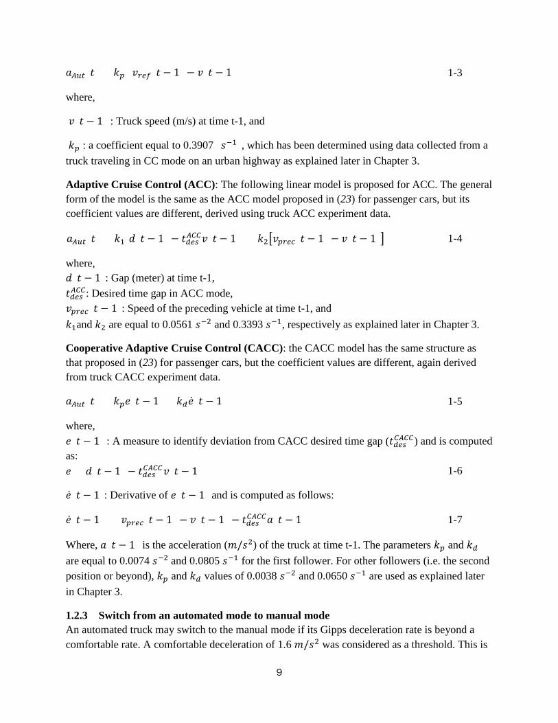
𝑎𝑎𝐶𝐶𝐴𝐴𝑡𝑡(𝑡𝑡) = 𝑘𝑘𝑝𝑝 (𝑣𝑣𝑡𝑡𝑡𝑡𝑓𝑓(𝑡𝑡 − 1) − 𝑣𝑣(𝑡𝑡 − 1)) 1-3

where,

𝑣𝑣(𝑡𝑡 − 1) : Truck speed (m/s) at time t-1, and

𝑘𝑘𝑝𝑝 : a coefficient equal to 0.3907 (𝑠𝑠−1), which has been determined using data collected from a truck traveling in CC mode on an urban highway as explained later in Chapter 3.

Adaptive Cruise Control (ACC): The following linear model is proposed for ACC. The general form of the model is the same as the ACC model proposed in (23) for passenger cars, but its coefficient values are different, derived using truck ACC experiment data.

𝑎𝑎𝐶𝐶𝐴𝐴𝑡𝑡(𝑡𝑡) = 𝑘𝑘1[𝑑𝑑(𝑡𝑡 − 1) − 𝑡𝑡𝑑𝑑𝑡𝑡𝑑𝑑𝐶𝐶𝐶𝐶𝐶𝐶𝑣𝑣(𝑡𝑡 − 1)] + 𝑘𝑘2�𝑣𝑣𝑝𝑝𝑡𝑡𝑡𝑡𝑝𝑝(𝑡𝑡 − 1) − 𝑣𝑣(𝑡𝑡 − 1)� 1-4

where, 𝑑𝑑(𝑡𝑡 − 1): Gap (meter) at time t-1, 𝑡𝑡𝑑𝑑𝑡𝑡𝑑𝑑𝐶𝐶𝐶𝐶𝐶𝐶: Desired time gap in ACC mode, 𝑣𝑣𝑝𝑝𝑡𝑡𝑡𝑡𝑝𝑝(𝑡𝑡 − 1): Speed of the preceding vehicle at time t-1, and 𝑘𝑘1and 𝑘𝑘2 are equal to 0.0561 𝑠𝑠−2 and 0.3393 𝑠𝑠−1, respectively as explained later in Chapter 3.

Cooperative Adaptive Cruise Control (CACC): the CACC model has the same structure as that proposed in (23) for passenger cars, but the coefficient values are different, again derived from truck CACC experiment data.

𝑎𝑎𝐶𝐶𝐴𝐴𝑡𝑡(𝑡𝑡) = 𝑘𝑘𝑝𝑝𝑒𝑒(𝑡𝑡 − 1) + 𝑘𝑘𝑑𝑑�̇�𝑒(𝑡𝑡 − 1) 1-5

where, 𝑒𝑒(𝑡𝑡 − 1) : A measure to identify deviation from CACC desired time gap (𝑡𝑡𝑑𝑑𝑡𝑡𝑑𝑑𝐶𝐶𝐶𝐶𝐶𝐶𝐶𝐶) and is computed as: 𝑒𝑒 = 𝑑𝑑(𝑡𝑡 − 1) − 𝑡𝑡𝑑𝑑𝑡𝑡𝑑𝑑𝐶𝐶𝐶𝐶𝐶𝐶𝐶𝐶𝑣𝑣(𝑡𝑡 − 1) 1-6

�̇�𝑒(𝑡𝑡 − 1): Derivative of 𝑒𝑒(𝑡𝑡 − 1) and is computed as follows:

�̇�𝑒(𝑡𝑡 − 1) = 𝑣𝑣𝑝𝑝𝑡𝑡𝑡𝑡𝑝𝑝(𝑡𝑡 − 1) − 𝑣𝑣(𝑡𝑡 − 1) − 𝑡𝑡𝑑𝑑𝑡𝑡𝑑𝑑𝐶𝐶𝐶𝐶𝐶𝐶𝐶𝐶𝑎𝑎(𝑡𝑡 − 1) 1-7

Where, 𝑎𝑎(𝑡𝑡 − 1) is the acceleration (𝑚𝑚/𝑠𝑠2) of the truck at time t-1. The parameters 𝑘𝑘𝑝𝑝 and 𝑘𝑘𝑑𝑑 are equal to 0.0074 𝑠𝑠−2 and 0.0805 𝑠𝑠−1 for the first follower. For other followers (i.e. the second position or beyond), 𝑘𝑘𝑝𝑝 and 𝑘𝑘𝑑𝑑 values of 0.0038 𝑠𝑠−2 and 0.0650 𝑠𝑠−1 are used as explained later in Chapter 3.

1.2.3 Switch from an automated mode to manual mode An automated truck may switch to the manual mode if its Gipps deceleration rate is beyond a comfortable rate. A comfortable deceleration of 1.6 𝑚𝑚/𝑠𝑠2 was considered as a threshold. This is

9

90% of 1.8 𝑚𝑚/𝑠𝑠2 which is the mean value for maximum deceleration. In addition, a truck will travel in manual mode if its speed is reduced to 3 𝑚𝑚/𝑠𝑠 (=10.8 km/h) or lower because the CACC system does not work at these lower speeds.

1.2.4 Desired speed computation Mean desired speed is assumed to be 𝑣𝑣𝑆𝑆𝐿𝐿 + 𝑣𝑣𝛿𝛿,𝑆𝑆𝐿𝐿 mph, where speed limits 𝑣𝑣𝑆𝑆𝐿𝐿 for cars and trucks are 65 mph and 55 mph, respectively and 𝑣𝑣𝛿𝛿,𝑆𝑆𝐿𝐿 is a calibration parameter. Desired speed may be adjusted due to the friction effect using the following equations.

𝑣𝑣𝑓𝑓𝑡𝑡𝑓𝑓𝑝𝑝𝑡𝑡𝑓𝑓𝑓𝑓𝑓𝑓(𝑡𝑡 − 1) = min{𝑣𝑣𝑙𝑙(𝑡𝑡 − 1), 𝑣𝑣𝑡𝑡(𝑡𝑡 − 1)} + 𝑣𝑣𝛿𝛿,𝑓𝑓𝑡𝑡𝑓𝑓𝑝𝑝𝑡𝑡𝑓𝑓𝑓𝑓𝑓𝑓 1-8

𝑣𝑣𝑑𝑑𝑡𝑡𝑑𝑑𝑓𝑓𝑡𝑡𝑡𝑡𝑑𝑑(𝑡𝑡) = �min�𝑣𝑣𝑓𝑓𝑡𝑡𝑓𝑓𝑝𝑝𝑡𝑡𝑓𝑓𝑓𝑓𝑓𝑓(𝑡𝑡 − 1),𝑉𝑉𝑆𝑆𝐿𝐿 + 𝑣𝑣𝛿𝛿,𝑆𝑆𝐿𝐿� 𝑀𝑀𝑖𝑖 𝑣𝑣(𝑡𝑡 − 1) > 𝑣𝑣𝑓𝑓𝑡𝑡𝑓𝑓𝑝𝑝𝑡𝑡𝑓𝑓𝑓𝑓𝑓𝑓

𝑉𝑉𝑆𝑆𝐿𝐿 + 𝑣𝑣𝛿𝛿,𝑆𝑆𝐿𝐿 𝑂𝑂𝑡𝑡ℎ𝑒𝑒𝑒𝑒𝑒𝑒𝑀𝑀𝑠𝑠𝑒𝑒 1-9

where,

𝑣𝑣𝑙𝑙(𝑡𝑡 − 1), 𝑣𝑣𝑡𝑡(𝑡𝑡 − 1) : the speeds of the left and right lanes, 𝑣𝑣𝛿𝛿,𝑓𝑓𝑡𝑡𝑓𝑓𝑝𝑝𝑡𝑡𝑓𝑓𝑓𝑓𝑓𝑓 : Speed difference between the subject lane and the adjacent lane and is a calibration parameter, 𝑣𝑣𝑓𝑓𝑡𝑡𝑓𝑓𝑝𝑝𝑡𝑡𝑓𝑓𝑓𝑓𝑓𝑓: Speed threshold below which friction effect is not implemented and is assumed to be 25 mph.

1.2.5 Lane changing models The lane changing model is similar to the models presented in (20-21). Additionally, this study considers a new type of mandatory lane change to make sure trucks are not traveling in the faster lanes. California restricts trucks to avoid using the left two lanes. In real traffic conditions, truck drivers may not restrict themselves to the lanes designated above. This may happen, for instance, when a truck passes a slower moving vehicle. In the current version of the simulation model, lane restriction criteria have been strictly applied so trucks never use the faster lanes, even to pass a slow moving vehicle.

1.2.6 Lane change cooperation Manual cars or trucks may reduce their speeds and create a longer gap to cooperate with vehicles merging from on-ramps. An automated truck may cooperate with merging vehicles if it is a CACC string leader, or it has previously disengaged the automated mode and is traveling in the manual mode. This implies that truck followers traveling in CACC mode do not deactivate the automated mode and do not disturb platoon stability to cooperate with merging vehicles.

Even with this setting, some passenger cars may cut-in between following trucks and interrupt a CACC string. A truck traveling behind a cut-in passenger car can travel in ACC mode, but if its

10

deceleration rate is beyond the comfortable deceleration rate of 1.6 𝑚𝑚/𝑠𝑠2, it will switch to the manual mode.

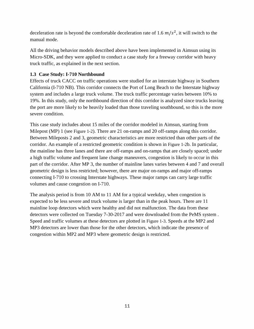
All the driving behavior models described above have been implemented in Aimsun using its Micro-SDK, and they were applied to conduct a case study for a freeway corridor with heavy truck traffic, as explained in the next section.

1.3 Case Study: I-710 Northbound Effects of truck CACC on traffic operations were studied for an interstate highway in Southern California (I-710 NB). This corridor connects the Port of Long Beach to the Interstate highway system and includes a large truck volume. The truck traffic percentage varies between 10% to 19%. In this study, only the northbound direction of this corridor is analyzed since trucks leaving the port are more likely to be heavily loaded than those traveling southbound, so this is the more severe condition.

This case study includes about 15 miles of the corridor modeled in Aimsun, starting from Milepost (MP) 1 (see Figure 1-2). There are 21 on-ramps and 20 off-ramps along this corridor. Between Mileposts 2 and 3, geometric characteristics are more restricted than other parts of the corridor. An example of a restricted geometric condition is shown in Figure 1-2b. In particular, the mainline has three lanes and there are off-ramps and on-ramps that are closely spaced; under a high traffic volume and frequent lane change maneuvers, congestion is likely to occur in this part of the corridor. After MP 3, the number of mainline lanes varies between 4 and 7 and overall geometric design is less restricted; however, there are major on-ramps and major off-ramps connecting I-710 to crossing Interstate highways. These major ramps can carry large traffic volumes and cause congestion on I-710.

The analysis period is from 10 AM to 11 AM for a typical weekday, when congestion is expected to be less severe and truck volume is larger than in the peak hours. There are 11 mainline loop detectors which were healthy and did not malfunction. The data from these detectors were collected on Tuesday 7-30-2017 and were downloaded from the PeMS system . Speed and traffic volumes at these detectors are plotted in Figure 1-3. Speeds at the MP2 and MP3 detectors are lower than those for the other detectors, which indicate the presence of congestion within MP2 and MP3 where geometric design is restricted.

11

Figure 1-2: a) I-710 NB corridor and loop detector locations (red bars) b) Location of the most congested detector modeled in Aimsun

Volume and speed information about this corridor is fairly limited. For the 15-mile corridor, there are only 11 healthy mainline detectors and these are not sufficient to accurately estimate ramp volumes. Thus, the initial O/D matrix was fine-tuned as part of the calibration process to replicate loop detector volumes. The parameter selection and calibration process will be explained in the next section.

1.3.1 Parameter selection Performance of trucks is governed by their limited acceleration/deceleration capabilities. The maximum acceleration rate depends on the weight-to-power ratio (w/p) and the speed of the truck. This study assumes w/p of 200 lb/hp to determine maximum acceleration rate. This w/p value was selected based on an NCHRP study (24) which reports 200 lb/hp as the 90th percentile value of w/p distribution for California interstate highways. Since trucks are mostly loaded in this corridor, the value of 200 lb/hp should be a good representative value. This study uses the corresponding acceleration values provided by the ITE handbook (25) as shown in Table 1-1.

12

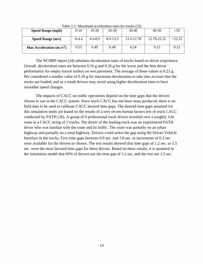
Table 1-1: Maximum acceleration rates for trucks (25) Speed Range (mph) 0-10 10-20 20-30 30-40 40-50 >50

Speed Range (m/s) 0-4.4 4.4-8.9 8.9-13.3 13.3-12.78 12.78-22.22 >22.22

Max Acceleration (𝐦𝐦/𝐬𝐬𝟐𝟐) 0.55 0.49 0.40 0.24 0.15 0.12

The NCHRP report (24) tabulates deceleration rates of trucks based on driver experience.

Overall, deceleration rates are between 0.16 g and 0.26 g for the worst and the best driver performance for empty tractor trailers on wet pavement. The average of these values is 0.21 g. We considered a smaller value of 0.18 g for maximum deceleration to take into account that the trucks are loaded; and as a result drivers may avoid using higher deceleration rates to have smoother speed changes.

The impacts of CACC on traffic operations depend on the time gaps that the drivers choose to use in the CACC system. Since truck CACC has not been mass produced, there is no field data to be used to calibrate CACC desired time gaps. The desired time gaps assumed for this simulation study are based on the results of a very recent human factors test of truck CACC conducted by PATH (26). A group of 9 professional truck drivers traveled over a roughly 3-hr route in a CACC string of 3 trucks. The driver of the leading truck was an experienced PATH driver who was familiar with the route and its traffic. The route was partially on an urban highway and partially on a rural highway. Drivers could select the gap using the Driver-Vehicle Interface in the trucks. Five time gaps between 0.9 sec. and 1.8 sec. in increments of 0.3 sec. were available for the drivers to choose. The test results showed that time gaps of 1.2 sec. or 1.5 sec. were the most favored time gaps for these drivers. Based on these results, it is assumed in the simulation model that 60% of drivers use the time gap of 1.2 sec, and the rest use 1.5 sec.

13

Figure 1-3: Comparison of simulation and field data at eleven detector stations for simulation using the calibrated parameter values

Another parameter is the desired time gap in ACC, which is expected to be longer than CACC time gaps since V2V communication is not available in ACC. An ACC desired gap of 1.8 sec has been implemented for trucks in Japan (7). This seems to be the lower end of available ACC gaps. We decided to assume a slightly larger desired gap of 2 sec for all trucks in ACC, which is in the middle range of commercially available ACC gap settings for heavy trucks.

010203040506070

Spee

d (m

ph)

Mile posts

Avg. Speed

Loop Simulation

4.3 0.9 1.2 5.0

1.7 2.6

0.1

3.8 3.6 1.3 0.8

0

1000

2000

3000

4000

5000

6000Vo

lum

e (v

eh/h

r)

Mile posts

Hourly Volume

Loop Simulation

14

1.3.2 Parameter calibration The Wisconsin DOT criteria, as presented in (27), were applied to calibrate the simulation model. A goodness of fit measure, proposed by Geoffrey E. Havers and called GEH, has been introduced to match traffic volume. GEH is defined in Equation 1-10 where 𝐿𝐿 and 𝑆𝑆 denote loop detector and simulated hourly volumes, respectively. In a good calibration, 85% of observations should have a GEH of 5 or less. The rest of the observations should not have a GEH of greater than 10.

𝐺𝐺𝐺𝐺𝐺𝐺 = �2(𝑆𝑆−𝐿𝐿)2

𝑆𝑆+𝐿𝐿 1-10

Figure 1-3 displays the loop detector volumes versus simulated traffic volumes with the corresponding GEH values on top of the bars. The simulated traffic volumes are computed based on 1 hr of simulation and 5 replications with different random number seeds. These simulated volumes have been derived after fine tuning O/D matrices and altering car following parameters such as reaction time. All the GEH values are either 5 or less, satisfying the GEH criteria.

For speed, Wisconsin DOT criteria suggest that speed be visually matched “to analysts’ satisfaction”. We decided to qualitatively match speed data because these data come from single loop detectors for which the G-factor computations involve approximations due to varying length of vehicles; as a result speed data are approximate values. Qualitative match would be sufficient for the purpose of this case study since its primary goal is comparing conditions with truck CACC versus manually driven trucks rather than designing specific alternatives for the study corridor.

Figure 1-3 also demonstrates simulated versus observed speeds which have been averaged over one hour. The average absolute error is equal to 4.36 mph, with a minimum of 0.63 mph and a maximum of 8.55 mph. In terms of traffic conditions, the simulated and the loop data are in close or acceptable agreement. MP2 and MP3 detectors demonstrate congested traffic conditions as both detectors show low speed. The rest of the detectors show higher speeds and free flow conditions.

The calibrated values of the car following parameters are shown in Table 1-2

1.4 Results The driver behavior models have been implemented in the Aimsun framework using their micro SDK, and simulations have been run for 5 replications with different random number seeds. Two scenarios are compared:

1) Base: All vehicles travel in manual mode, and 2) 100% Truck CACC: Passenger cars travel in manual mode, but all trucks have CACC

vehicle following capability

15

Table 1-2: Calibrated values of car following parameters Parameter Mathematical Symbol Calibrated value Reaction time 𝜏𝜏𝑡𝑡 1.3 sec Desired time gap for manual trucks 𝜏𝜏 2.4 sec Desired time gap for manual cars 𝜏𝜏 1.25 sec Theta 𝜃𝜃 0.2* 𝜏𝜏𝑡𝑡=0.26 Max Acceleration for cars 𝑎𝑎𝑀𝑀 2.5 𝑚𝑚/𝑠𝑠2 Max Deceleration for cars 𝑏𝑏𝑓𝑓 3 𝑚𝑚/𝑠𝑠2 Minimum speed difference to consider friction effect

𝑣𝑣𝑓𝑓𝑡𝑡𝑓𝑓𝑝𝑝𝑡𝑡𝑓𝑓𝑓𝑓𝑓𝑓 ,𝛿𝛿 10 m/s

Difference between speed limit and average desired speed

𝑣𝑣𝑆𝑆𝐿𝐿 ,𝛿𝛿 3 m/s

1.4.1 Corridor analyses Truck CACC increased Vehicle Mile Traveled (VMT) and average speed for both trucks and passenger cars. For trucks, average VMT increased from 10.7 × 103 to 11.4 × 103 representing a 5.8% increase; and average speed increased from 33.3 mph to 39.7 mph, a 19.3% increase. Average speed was computed as VMT divided by Vehicle Time Traveled (VTT). For cars, VMT and average speed increased by 0.7% and 6.2%, respectively.

The main reason for these improvements is that truck CACC reduced congestion near the beginning of the corridor, which improved mobility of passenger cars as well. In addition, truck CACC increased truck speeds in the uncongested conditions; thus passenger cars which get stuck behind trucks or follow them could travel faster than in the Base condition. These effects are discussed further in the next sections of this chapter.

1.4.2 Analyses at individual loop detector locations Figure 1-4 displays flow rate and speed of trucks with and without truck CACC for the loop detectors used in the model calibration. All the detector stations show speed increases ranging from 1.84 mph to 9.26 mph. In order to provide better understanding of the character of the speed changes, Figure 1-5 plots speed increase values versus speed values in the Base case for the eleven detector stations. The plot shows that speed increase values are noticeably larger for the two detectors that had average speeds below 30 mph and that had persistent flow breakdowns

16

Figure 1-4: Effects of truck CACC at eleven detector stations for cars and trucks

a) Hourly Average Speed - Trucks b) Hourly Volume – Trucks

0

10

20

30

40

50

60

Spee

d (m

ph)

Mile posts

Hourly Avg. Speed - Truck

0% CACC 100% Truck CACC

-2%

0%

2%

4%

6%

8%

10%

0

200

400

600

800

1000

1200

% C

hang

e

Volu

me

(veh

/hr)

Mile posts

Hourly Volume - Truck

0% CACC 100% Truck CACC % Change

0

20

40

60

80

Spee

d (m

ph)

Mile posts

Hourly Avg. Speed - Cars

0% CACC 100% Truck CACC

-2%

0%

2%

4%

6%

8%

10%

0

1000

2000

3000

4000

5000

6000

% C

hang

e

Volu

me

(veh

/hr)

Mile posts

Hourly Volume - Cars

0% CACC 100% Truck CACC % Change

c) Hourly Average Speed-Cars d) Hourly Volume - Cars

17

in the Base condition. The speed increase values are larger because truck CACC reduced congestion severity by postponing the onset of congestion, and this resulted in much larger speed increases.

Figure 1-4 illustrates that truck flow rates increased between 2.1% and 8.3%. This could be because of the speed increases discussed above as well as shorter following gaps in CACC.

Also, it could be interesting to see how truck CACC affects passenger car mobility. Figure 1-4 suggests that overall, there is no drawback and at some detector locations truck CACC considerably improved passenger car mobility. In particular, flow rate increased by 0.04% to 1.8%, and average speed increased between 0.11 mph and 3.85 mph. These statistics represent the effects of truck CACC on cars’ mobility averaged over five replications, with considerable variability across replications. For instance, the MP2 detector had the lowest average flow rate improvement. For two replications, the volume of passenger cars decreased by 8 and 17 cars, but for the other three replications, it increased by 4, 15, and 13 cars. This led to an overall increase of 0.04% in flow rate. Thus at an aggregate level, the study concluded that truck CACC did not diminish passenger cars’ mobility.

Figure 1-5: Speed increase due to truck CACC versus base case speed plotted for eleven detector stations

1.4.3 Detailed analyses for selected loop detector stations To provide more insight about the dynamics of truck flow and speed, temporal changes of traffic variables are presented for the detector stations at MP2 and MP12.

The MP2 detector was chosen because it had the lowest speed in the Base condition, indicating congestion. Two merge areas influence the traffic data collected by this loop detector. The first merge area is where the detector has been placed and the second is 270 m downstream of the detector location. The flow disturbance is mainly caused by vehicles that try to enter the

0

2

4

6

8

10

0 10 20 30 40 50 60

Spee

d In

crea

se D

ue to

T

ruck

CA

CC

(mph

)

Truck Speed at Base (mph)

18

rightmost lane from the on-ramps. The mainline has three lanes at these two locations, and trucks are restricted to use only the rightmost lane, but passenger cars may use this lane as well.

Figure 1-6 depicts how speed and flow rate change every 5 minutes. For a given 5-minute interval and a given replication, average speed and flow rate were computed. Then, these values were again averaged over 5 replications (with different random seeds) and depicted in Figure 1-6. . Speed data in Figure 1-6a show that speed varies between 12.48 mph and 21.6 mph for 0% CACC indicating presence of congestion at MP2. With 100% truck CACC, average speed varied between 17.77 mph and 55.22 mph indicating a significantly higher speed compared with 0% truck CACC.

Figure 1-6a also displays speed variations for two individual replications as well as the average values, and it shows similar traffic patterns were reproduced across replications. Thus, average values could be considered representative of expected congestion trends.

The MP10 detector station was chosen to represent a location with free flow conditions, as its average speed in the Base case was 52.58 mph. It is located on a 4-lane section of the highway between an upstream off-ramp and a downstream on-ramp, but ramp volumes were not high enough to create a disturbance at this location. The detector distance to the upstream off-ramp is about 600 m, and its distance to the downstream on-ramp is about 200 m.

Figure 1-6 shows that at MP10 truck speeds with CACC are greater than those in the Base condition by 3.65 mph to 9.94 mph, with an average of 6.24 mph. The flow rate is larger by 12 truck/hr to 112.8 truck/hr with an average of 47.8 truck/hr.

1.5 Conclusions This study has shown how traffic micro-simulation, based on well-calibrated models of human driver behavior and of automatic vehicle following dynamics, can be used to represent the traffic impacts of widespread use of CACC on heavy trucks. The simulation method includes several innovative features derived directly from truck CACC experiments. It incorporates truck following models which have been recently developed for the separate automated modes of CACC, ACC, and CC. The simulation logic includes switching from one automated mode to another and deactivation of automation to travel in manual mode. It also applies the results of a gap acceptance test recently conducted by PATH for truck drivers using CACC to select time gaps of 1.2 sec. and 1.5 sec. for use in the simulation. The simulation includes behavioral models such as models for lane change maneuvers, lane change cooperation, and lane use restriction for trucks; thus it can realistically represent traffic dynamics such as cut-in and cut-out vehicles as well as lane change cooperation by automated truck drivers.

A case study was conducted for a 15-mile urban corridor which experienced both congested and uncongested conditions during a one-hour simulation. Results of five simulation replications showed that 100% truck usage of CACC improved traffic operations for trucks and cars at different locations. In particular, truck CACC could postpone the onset of congestion, and it

19

could increase traffic speed at some uncongested locations. Corridor level analysis for trucks demonstrated that average speed increased from 33.3 mph to 39.7 mph, and VMT increased by 5.8%. The results also showed that truck CACC did not adversely affect traffic operations for cars, and at some locations it even brought a significant speed increase. Corridor level analysis for cars showed that their average speed increased from 49.3 mph to 52.4 mph, and VMT increased by 0.7%.

This simulation method can be used in future studies to further characterize impacts of truck CACC on traffic flow and energy consumption and to explore management strategies which enhance benefits of truck platooning. Thus at future steps, effects of market penetration rate and gap acceptance on traffic operations will be explored. The current simulation will also be extended to study impacts of truck CACC on energy consumption.

20

Figure 1-6: Speed and flow rate variations over time for two loop detectors

0

10

20

30

40

50

60

70

1 6 11

Truc

k sp

eed

(mph

)

5-min Interval Index 100% Truck CACC (Avg) 0% CACC (Avg)

c) MP 10 Detector - Speed d) MP 10 Detector – Flow Rate

a) MP 2 Detector - Speed b) MP 2 Detector – Flow Rate

Replication 1

Replication 2

0

10

20

30

40

50

60

70

1 6 11

Truc

k sp

eed

(mph

)

5-min Interval Index 100% Truck CACC 0% CACC

0100200300400500600700800

1 6 11

Truc

k flo

w ra

te (v

eh/h

r)

5-min Interval Index 100% Truck CACC 0% CACC

0100200300400500600700800

1 3 5 7 9 11

Truc

k flo

w (v

eh/h

r)

5-min Interval Index 100% Truck CACC 0% CACC

21

Chapter 2 Effect of Truck Platooning on Energy Consumption One of the potential benefits of truck platooning is energy saving. The underlying idea is that followers would experience less aerodynamic drag and as a result consume less energy. Energy saving due to platooning has been measured and reported in several experimental studies (5-12). During past experimental studies, truck speed and time gap were constant and platoon characteristics did not practically vary; however in the real world they do vary. For instance, a platoon speed may vary due to presence of a slow moving vehicle in front of the lead truck, or intra platoon gaps may not stay the same when a cut-in maneuver occurs. These traffic dynamics can influence energy consumption, and their effects need to be studied. In this chapter a method to estimate energy consumption is proposed and integrated with the micro simulation model developed in the previous chapter.

The proposed method is a modified version of the Motor Vehicle Emission Simulator (MOVES) model. MOVES is a computer program which is used within the Environmental Protection Agency (EPA) to estimate energy consumption and resulting emission impacts for different types of vehicles including cars and trucks. MOVES does not consider the effect of truck platooning on aerodynamic drag reduction and energy saving; thus modifications should be implemented to incorporate the effect of truck platooning. In this section, the MOVES approach to estimate energy consumption is illustrated, and then modifications are proposed to incorporate the effect of truck platooning.

This chapter is organized as following: first over view of MOVES is presented, and then its modifications are proposed. Case study results are discussed followed by conclusions.

2.1 MOVES Overview

EPA provided various documents explaining MOVES, including user manual, technical background, modifications in different versions and training courses; and these documents can be mainly found in the MOVES webpage (28). One may refer to these documents for detailed descriptions. In this section, an overview of the MOVES model is presented when second-by-second speed and acceleration data are available to estimate energy consumption.

2.1.1 Energy consumption for passenger cars

The key parameter to estimate energy consumption rate is Vehicle Specific Power (VSP), which is considered as the required tractive power to move a vehicle, normalized by mass. Vehicle Specific Power at time t (𝑉𝑉𝑆𝑆𝑃𝑃𝑡𝑡) is computed as:

𝑉𝑉𝑆𝑆𝑃𝑃𝑡𝑡 = 𝐶𝐶𝑣𝑣𝑡𝑡+𝐵𝐵𝑣𝑣𝑡𝑡2+𝐶𝐶𝑣𝑣𝑡𝑡3+𝑀𝑀𝑣𝑣𝑡𝑡(𝑚𝑚𝑡𝑡+𝑡𝑡 𝑑𝑑𝑓𝑓𝑓𝑓𝜃𝜃)𝑀𝑀

2-1

Where, 𝑣𝑣𝑡𝑡: Velocity (𝑚𝑚/𝑠𝑠) at time t,

22

𝑎𝑎𝑡𝑡: Acceleration (𝑚𝑚/𝑠𝑠2) at time t, 𝑔𝑔: Gravitational acceleration (𝑚𝑚/𝑠𝑠2) which is equal to 9.8 𝑚𝑚

𝑑𝑑2,

𝜃𝜃: Road grade, 𝑀𝑀: Mass of the vehicle (metric ton). MOVES suggests 1.4788 tones for the typical weight of a passenger car (29). 𝐴𝐴,𝐵𝐵, and 𝐶𝐶: Road load coefficients. According to (29) “𝐴𝐴 is associated with tire rolling resistance, 𝐵𝐵 with mechanical rotating friction as well as higher order rolling resistance losses, and 𝐶𝐶 with aerodynamic drag”. This statement should not be generalized for trucks because, as it will be elaborated later, 𝐶𝐶 also includes the second order rolling resistance for trucks. MOVES

suggests typical coefficient values of 0.156461 𝐾𝐾𝐾𝐾−𝑑𝑑𝑚𝑚

, 0.002002 𝐾𝐾𝐾𝐾−𝑑𝑑2

𝑚𝑚2 , and 0.000493 𝐾𝐾𝐾𝐾−𝑑𝑑3

𝑚𝑚3 for passenger cars, respectively.

Once 𝑉𝑉𝑆𝑆𝑃𝑃𝑡𝑡 is computed, one needs to determine the vehicle operating mode MOVES defined 23 operating modes. The operating mode 0 represents stopped vehicles (speed less than 1 mph) and the operating mode 1 represents braking conditions ( braking rate < -0.4 𝑚𝑚

𝑑𝑑2). If a vehicle does not

have an operating mode of 0 or 1, its operating mode is determined based on its speed and 𝑉𝑉𝑆𝑆𝑃𝑃𝑡𝑡 as demonstrated in the table of Figure 2-1a. In particular, each column of the table represents a speed class and each row represents a VSP class, and values inside the cells indicate the corresponding operating mode. For instance, the operating mode for VSP of 2 𝐾𝐾𝐾𝐾

𝑡𝑡𝑓𝑓𝑓𝑓𝑡𝑡 and speed of

30 mph will be 22 (unit-less). The energy consumption corresponding to this operating mode can be read from the vertical axis of Figure 2-1b.

Figure 2-1: Determination of a) operating modes and b) energy consumption rates for passenger cars

0

1

2

3

4

5

6

7

8

0 10 20 30 40

Ene

rgy

Rat

e (K

J/hr

) 10^

5

Operating Mode

23

2.1.2 Energy consumption for diesel trucks

Instead of VSP, a similar measure called Scaled Tractive Power (STP) is computed for trucks as:

𝑆𝑆𝑆𝑆𝑃𝑃𝑡𝑡 = 𝐶𝐶𝑣𝑣𝑡𝑡+𝐵𝐵𝑣𝑣𝑡𝑡2+𝐶𝐶𝑣𝑣𝑡𝑡3+(𝑀𝑀𝑣𝑣𝑡𝑡𝑚𝑚𝑡𝑡+𝑡𝑡 𝑑𝑑𝑓𝑓𝑓𝑓𝜃𝜃)𝑓𝑓𝑠𝑠𝑠𝑠𝑠𝑠𝑠𝑠𝑠𝑠

2-2

where, 𝑖𝑖𝑑𝑑𝑝𝑝𝑚𝑚𝑙𝑙𝑡𝑡 is equal to 17.1 tons. The road load coefficients can be calculated using equations 2-3 to 2-5 (30).

𝐴𝐴 = 𝐶𝐶𝑅𝑅0𝑀𝑀𝑔𝑔 2-3 𝐵𝐵 = 0 2-4

𝐶𝐶 = 𝐶𝐶𝐷𝐷𝐶𝐶𝑓𝑓𝜌𝜌𝑠𝑠𝑎𝑎𝑎𝑎2

+ 𝐶𝐶𝑅𝑅2𝑀𝑀𝑔𝑔 2-5 where, 𝐶𝐶𝑅𝑅0 and 𝐶𝐶𝑅𝑅2: The zero and the second order rolling resistance force terms, 𝐶𝐶𝐷𝐷: Drag coefficient, 𝐴𝐴𝑓𝑓: Frontal area of the tractor-trailer, and 𝜌𝜌𝑚𝑚𝑓𝑓𝑡𝑡: Air density,

Although MOVES reports typical values of the coefficients in (29), the current study computes coefficients based on the specifics of the trucks used in our experiment. This would provide more consistency as experimental results will be later used to re-calibrate coefficients for followers. The following values will be used based on our test truck specifics to compute road load coefficients. (11)

𝑀𝑀 = 29.5 × 103 𝑘𝑘𝑔𝑔 𝐶𝐶𝑅𝑅0 = 0.006 𝐶𝐶𝐷𝐷 = 0.57 𝐴𝐴𝑓𝑓 = 10.7 𝑚𝑚2

𝜌𝜌𝑚𝑚𝑓𝑓𝑡𝑡 = 1.2 𝑘𝑘𝑡𝑡𝑚𝑚3

2-6

The value of 𝐶𝐶𝑅𝑅2 is determined based on (30) and is equal to 0.43 × 10−5. Thus, the values of road load coefficients will be:

𝐴𝐴 = 1.74 𝐾𝐾𝐾𝐾−𝑑𝑑𝑚𝑚

, 𝐵𝐵 = 0 𝐾𝐾𝐾𝐾−𝑑𝑑2

𝑚𝑚2 , and 𝐶𝐶 = 0.0049 𝐾𝐾𝐾𝐾−𝑑𝑑3

𝑚𝑚3 2-7

Once STP is calculated, an operating mode is determined using the same approach described for passenger cars. For each operating mode, energy consumption rates will be read from Figure 2-2.

24

Figure 2-2: Energy consumption rates for diesel trucks

2.2 MOVES Modifications The underlying idea behind truck platooning is that followers in a platoon experience less aerodynamic drag. A decrease in aerodynamic drag can be reflected in STP computations by choosing a smaller value for coefficient C, which incorporates the drag coefficient (see Equation 2-2). In this study, the process of determining the value of C using experiment data is called MOVES re-calibration.

The re-calibration data were measured during an experiment conducted by PATH and Transport Canada (11). As a part of this project, the effects of time gap, position in platoon, and type of trailer were studied for a 3-truck platoon, and the corresponding energy savings have been plotted in Figure 2-3.

The current study focuses on trucks with a standard dry goods box trailer. Based on these data, the leader is not considerably influenced by platooning. Both middle and trailing trucks significantly save energy, but the benefit is larger for the trailing truck than the middle truck. Data for four different time gaps show that the energy saving for time gap of 0.6 sec is larger than for the other (longer) time gaps.

The experiment results are projected for the comparable conditions, which may happen in the simulation, as shown in Table 2-1. The results are extrapolated up to a gap of 2 seconds. Beyond this gap platooning may or may not result in measurable energy saving and this should be tested in experiments. Data in Table 2-1 are used to re-calibrate MOVES such that it returns the same energy savings for the experiment conditions.

0

1

2

3

4

5

6

7

8

0 10 20 30 40

Ene

rgy

Rat

e (K

J/hr

) 10^

6

Operating Mode

25

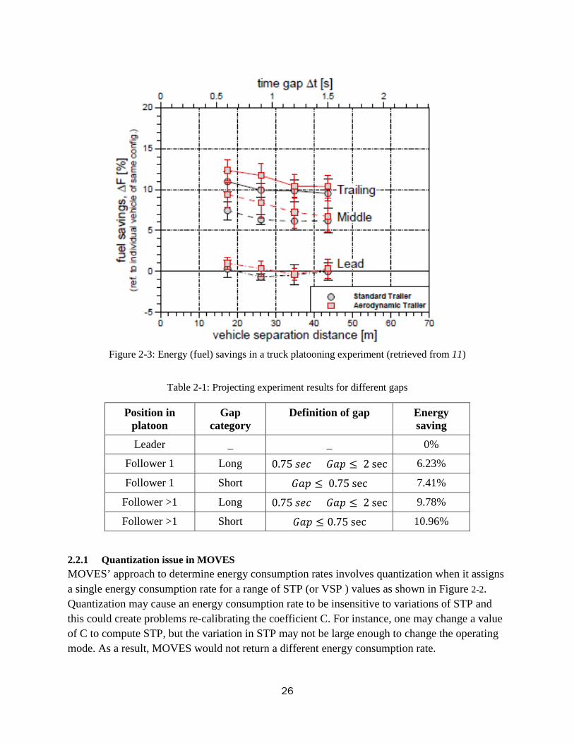
Figure 2-3: Energy (fuel) savings in a truck platooning experiment (retrieved from 11)

Table 2-1: Projecting experiment results for different gaps

Position in platoon

Gap category

Definition of gap Energy saving

Leader _ _ 0%

Follower 1 Long 0.75 𝑠𝑠𝑒𝑒𝑠𝑠 < 𝐺𝐺𝑎𝑎𝐺𝐺 ≤ 2 sec 6.23%

Follower 1 Short 𝐺𝐺𝑎𝑎𝐺𝐺 ≤ 0.75 sec 7.41%

Follower >1 Long 0.75 𝑠𝑠𝑒𝑒𝑠𝑠 < 𝐺𝐺𝑎𝑎𝐺𝐺 ≤ 2 sec 9.78%

Follower >1 Short 𝐺𝐺𝑎𝑎𝐺𝐺 ≤ 0.75 sec 10.96%

2.2.1 Quantization issue in MOVES MOVES’ approach to determine energy consumption rates involves quantization when it assigns a single energy consumption rate for a range of STP (or VSP ) values as shown in Figure 2-2. Quantization may cause an energy consumption rate to be insensitive to variations of STP and this could create problems re-calibrating the coefficient C. For instance, one may change a value of C to compute STP, but the variation in STP may not be large enough to change the operating mode. As a result, MOVES would not return a different energy consumption rate.

26

In order to manage this issue, the relationship between energy consumption rates and STPs has been smoothed. In particular, it is assumed that the energy consumption rates in Figure 2-2 represent mid-STP values. For the rest of the STP values, energy consumption rates are determined by interpolation or extrapolation. As a result, any variations in road load parameters and STP values would be reflected in the computed energy consumption rates.

To re-calibrate parameter C, energy consumption rates versus STPs have been interpolated continuously, as shown in Figure 2-4 , for speed class of 50 mph or faster because the trucks’ speed in the experiment was 65 mph and falls in this class. Based on the road load coefficient in Equation 2-2, a single truck in the experiment conditions would have a STP of 10.08 𝐾𝐾𝐾𝐾

𝑡𝑡𝑓𝑓𝑓𝑓 and a

corresponding energy consumption rate of 16.41 × 106𝑘𝑘𝑘𝑘/ℎ𝑒𝑒. If C value of 0.425 is selected, the corresponding STP and energy rate will be equal to 9.32 𝐾𝐾𝐾𝐾

𝑡𝑡𝑓𝑓𝑓𝑓 and 14.61× 106𝑘𝑘𝑘𝑘/ℎ𝑒𝑒,

respectively. These values correspond to 10.96% energy saving, which was reported for the trailing truck with a short time gap.

Similar numerical procedures were conducted to obtain C values for different positions in the platoon and different time gaps. Results are shown in Table 2-2.

Figure 2-4: Energy consumption rates for diesel trucks interpolated and smoothed in speed Class 3

0

10

20

30

40

50

60

0 5 10 15 20 25 30 35

Ene

rgy

Rat

e (K

J*10

^5/h

r)

Scaled Tractive Power

MOVES model continuumized Single truck

A follower with 11% energy saving

27

Table 2-2: Re-calibrated values for road load coefficient C

Position in platoon Gap category

Energy saving

Re-calibrated road load coefficient

Estimated drag coefficients

Leader _ 0% 0.0049 0.57

Follower 1 Long 6.23% 0.004375 0.488

Follower 1 Short 7.41% 0.004272 0.472

Follower >1 Long 9.78% 0.004073 0.441

Follower >1 Short 10.96% 0.00397 0.425

2.2.2 Energy consumption reduction factors for different operating modes In the experiment, trucks had a constant speed of 65 mph, but in the simulation they may accelerate or decelerate due to a variety of traffic conditions such as joining the queue, departing the queue or responding to a cut-in vehicle. Thus in simulation, trucks would not have the same speed as in the experiment; as a result, energy consumption reduction rates should be projected for other conditions which have not been covered in the experiment. Energy consumption reduction factors are projected using the re-calibrated C values assuming that drag coefficients do not considerably alter as a function of speed.

For operating modes 0 and 1, it is assumed that there is no energy saving due to aerodynamic drag reduction because operating mode 0 represents stopped condition and operating mode 1 represents braking conditions with a rate of 0.4 𝑚𝑚

𝑑𝑑𝑠𝑠 or more severe. Aerodynamic drag reduction is

not considered, as engine power would not be used in these operating modes.

For the other operating modes, the core idea is to compare energy consumption rates for a single truck versus those for a follower and compute energy reduction factors for the follower. In particular, an energy consumption rate for a single truck is computed when its combination of speed and acceleration returns the mid-STP value of a given operating mode. Then, another energy consumption rate for a follower is computed when its speed and acceleration are the same as those for the single truck, but its road load coefficient C is smaller and comes from Table 2-2.

The core idea needs to be further polished to address variability of reduction factors. There could be different combinations of speed and acceleration returning a mid STP value. These different combinations would return different reduction factors. For instance, a smaller reduction factor would be computed for a truck with a lower speed because a smaller portion of STP would be due to aerodynamic effect and a larger portion originates from acceleration. Thus reduction factors could vary based on speed even if STP is fixed. To address this variability issue, two

28

reduction factors are computed for the smallest and the largest speeds of a given operating mode, and the average of the two reduction factors will be used for that operating mode.

The following step-by-step procedure explains computations of reduction factors for a given operating mode. Road-load coefficients A and B are the same for a leader and followers; thus they stay the same throughout the computations and their values will be equal to the parameter values presented in 2-7. Hence the procedure is presented using simplified notations as if STP is a function of acceleration 𝑎𝑎, speed 𝑣𝑣 and coefficient C.

Step-by-step procedure to compute a reduction factor for a given operating mode Step 0: Define: 𝑣𝑣 and 𝑣𝑣 : smallest and largest speeds for the given operating mode. 𝐶𝐶𝑑𝑑 and 𝐶𝐶𝑓𝑓: Values of road load coefficient C for a single truck and a follower truck, respectively, and 𝑆𝑆𝑆𝑆𝑃𝑃𝑚𝑚𝑓𝑓𝑑𝑑: Mid STP value for the operating mode. Step 1: Use Equation 2-2 to compute acceleration rate 𝑎𝑎 for a single truck with speed of 𝑣𝑣 and 𝑆𝑆𝑆𝑆𝑃𝑃𝑚𝑚𝑓𝑓𝑑𝑑: 𝑎𝑎 = arg [ 𝑆𝑆𝑆𝑆𝑃𝑃�𝑎𝑎, 𝑣𝑣,𝐶𝐶 |𝑣𝑣 = 𝑣𝑣,𝐶𝐶 = 𝐶𝐶𝑑𝑑� = 𝑆𝑆𝑆𝑆𝑃𝑃𝑚𝑚𝑓𝑓𝑑𝑑] 2-8 Step 2: Compute 𝑆𝑆𝑆𝑆𝑃𝑃𝑓𝑓 which is the STP value for the follower with the same acceleration and speed and a smaller value for C. The value of C depends on the follower position in the platoon and its gap as tabulated in Table 2-2: 𝑆𝑆𝑆𝑆𝑃𝑃𝑓𝑓 = 𝑆𝑆𝑆𝑆𝑃𝑃(𝑎𝑎, 𝑣𝑣,𝐶𝐶|𝑎𝑎 = 𝑎𝑎, 𝑣𝑣 = 𝑣𝑣,𝐶𝐶 = 𝐶𝐶𝑓𝑓) 2-9 Step 3: Use smoothed relationship between STP and energy consumption rates to compute energy consumption rates corresponding to 𝑆𝑆𝑆𝑆𝑃𝑃𝑚𝑚𝑓𝑓𝑑𝑑 and 𝑆𝑆𝑆𝑆𝑃𝑃𝑓𝑓; and denote them as 𝐺𝐺(𝑆𝑆𝑆𝑆𝑃𝑃𝑚𝑚𝑓𝑓𝑑𝑑), and 𝐺𝐺�𝑆𝑆𝑆𝑆𝑃𝑃𝑓𝑓�, respectively. Step 4: Compute reduction factor 𝑅𝑅 corresponding to a follower traveling with speed of 𝑣𝑣

𝑅𝑅 = 𝐸𝐸(𝑆𝑆𝑆𝑆𝑃𝑃𝑚𝑚𝑎𝑎𝑚𝑚)−𝐸𝐸�𝑆𝑆𝑆𝑆𝑃𝑃𝑓𝑓�𝐸𝐸(𝑆𝑆𝑆𝑆𝑃𝑃𝑚𝑚𝑎𝑎𝑚𝑚) 2-10

Step 5: Repeat the Steps 1 to 4 to compute 𝑅𝑅 when 𝑣𝑣 =𝑣𝑣 Step 6: Compute average reduction factor:

𝑅𝑅 = (𝑅𝑅+𝑅𝑅)2

2-11

29

The same steps should be repeated for all operating modes and different values of 𝐶𝐶𝑓𝑓 presented in Table 2-2.

In the computations above, computed 𝑅𝑅 (or 𝑅𝑅) for operating modes 21 and 31 were capped by the measured values in Table 2-1. This is to avoid overestimation of reduction factors where there is no data to support larger reduction factors.

Figure 2-5 shows the reduction factors computed for the middle truck and the trailing truck with a long gap. Reduction factors for the trucks with a short gap are similar to those with a long gap and were not depicted in this chart. For a given speed class, there is a decreasing trend in reduction factors. As operating mode increases, STP increases, and this increase is mainly due to a larger acceleration rate. As a result the portion of aerodynamic effect in STP calculation becomes smaller and platooning would be effective at reducing a smaller portion of the STP.

Figure 2-5: Projected energy savings for different operating modes

2.3 Case Study The effect of truck platooning on energy consumption is studied for the I-710 NB corridor introduced in the previous chapter. Five simulation replications, with different random seeds, were run to compare these scenarios:

1- No truck CACC which is called the Base scenario, and 2- 100% truck CACC

0.0%

2.0%

4.0%

6.0%

8.0%

10.0%

12.0%

0 5 10 15 20 25 30 35 40 45

% e

nerg

y sa

ving

in p

lato

on

Operating mode

Middle truck w/ Long gap Trailing truck w/ Long gap

30

In the following sections, corridor level analysis is discussed; and then link level analysis, which provides more detailed description of results, is presented.

2.3.1 Corridor level analysis

Energy saving for different vehicle type: For each vehicle type, total consumed energy was normalized by the corresponding Vehicle-Mile-Traveled (VMT). Results showed that truck CACC reduced normalized energy consumption by 2.57% to 3.60% with the average of 3.05% over five replications. This corresponds to a fuel economy increase of 3.14% in miles per gallon. The average energy consumption for cars was slightly increased, by 0.26%, which can be considered as negligible energy consumption sensitivity.

The effect of truck CACC on energy consumption can be associated with two sources: 1) Aerodynamic effect 2) Speed change effect. In Figure 2-6, energy savings are partitioned to demonstrate the portions associated with these two sources. The speed change is associated with average energy consumption reduction of 2.57% and it varies between 2.09% and 3.11% over different runs. The aerodynamic effect is associated with average energy consumption reduction of 0.48% and this does not considerably vary over the different runs. For this specific corridor and traffic condition, the benefit from speed change is larger than the benefit from aerodynamic drag reduction by a factor of 5.35 (= 2.57%

0.48%).

The energy saving due to aerodynamic drag reduction depends on the platooning pattern, in the sense that what percent of truck-time-traveled was in a platoon and what time gaps have been selected in the platoon. The next section will closely explore platooning patterns in the corridor.

31

Figure 2-6: I-710 simulation results: estimated energy saving for different replications

Platooning pattern: Table 2-3 shows the percentage of truck-time-traveled for different platooning conditions for one simulation replication. Two categories do not experience energy consumption reduction due to platooning. They are 1) leaders and 2) followers braking or stopped, and these are corresponding to operating modes number 0 and 1 in Figure 2-1. For these two operating modes aerodynamic drag reduction was not considered since engine power is not used. These categories together represent 84.28% of truck-time-traveled. The rest (i.e. 15.72%) was used in computations to determine the effect of platooning on aerodynamic drag reduction. This fraction is called degree of Aerodynamically Efficient Platooning (AEP). Degree of AEP is introduced, instead of degree of platooning, to highlight that followers with operating modes of 0 or 1 are excluded from analysis. “It should be noted that 15.72% is the degree of AEP for the ad-hoc platooning strategy that was simulated, with no specific speed control or lane change strategies used to create new platoons or to keep platoons stable. In order to increase this degree specific algorithms should be developed to help CACC equipped trucks find each other and increase the degree of AEP.”

Based on Table 2-3, most of AEP belongs to followers with long gaps and this is expected as the desired gap was set to be 1.2 sec or 1.5 sec. Also, the percentage of AEP for follower1 is larger than that for follower >1 by a factor of larger than 2, which implies that most of AEP comes from 2-truck platoons (including the leader).

In the link level analysis, the effect of degree of AEP on energy saving is explored.

2.98% 3.11%

2.09% 2.52%

2.16% 2.571%

0.47% 0.49%

0.47%

0.46%

0.48%

0.48%

0%

1%

2%

3%

4%

Run1 Run2 Run3 Run4 Run5 Avg

% E

nerg

y Sa

ve p

er V

MT

Speed change effect Aerodynamic effect

32

Table 2-3: Platooning pattern in one simulation run Platooning category Short gap Long gap

Leader 76.24%

Followers braking or stopped 8.04%

Follower 1 0.07% 11.76%

Follower >1 0.02% 3.86%

2.3.2 Link level analysis In this section, we see how truck CACC influenced energy consumption for only mainline links because variations in degree of platooning and traffic speed are more noticeable on these links, and drivers on the mainline have different behavior than drivers on ramps.

Aerodynamic effect: Figure 2-7a shows the magnitude of normalized energy saving (i.e. divided by VMT) versus percentage of AEP when each point represents a link. AEPs are all below 30% and the data shows a strong linear correlation, with 𝑅𝑅2 of 0.85. It seems that for these simulation data, knowing the degree of AEP would be sufficient to predict energy consumption reduction due to the reduced aerodynamic drag effect.

Figure 2-7b shows energy saving versus link speeds to explore how energy saving varies based on traffic conditions. One may divide the data into two clusters. One cluster belongs to lower speeds (≤ 35 mph) demonstrating lower values of energy saving. The degree of EAP is smaller for these links because speed is low and gaps between trucks are mostly larger than 2 seconds. The next cluster demonstrates energy saving for higher speeds (>35 mph) with more scatter than for lower speeds. The scatter is mostly related to variations in degree of AEP as they have strong correlation with energy saving as depicted in Figure 2-7a. Thus, the majority of the energy saving comes from links with a speed above 35 mph.

Figure 2-7: Aerodynamic energy saving for links versus a) degree of AEP, and b) average truck speed

y = 832.05x R² = 0.8507

0

50

100

150

200

250

300

0.0% 10.0% 20.0% 30.0%

Ene

rgy

savi

ng (

KJ/

VM

T)

% AEP

0

50

100

150

200

250

300

0 10 20 30 40 50 60

Ene

rgy

savi

ng (

KJ/

VM

T)

Avg. truck speed (mph)

33

Speed change effect: Truck CACC increased average traffic speed from 33.3 mph to 39.7 mph and resulted in average energy saving of 2.57%. Although the net effect of truck CACC was a energy consumption reduction for the whole corridor, this trend may not be the case for some of the links. Figure 2-8a shows histograms for links that experienced energy consumption reduction and increase, separately. The frequency of links with energy reduction is larger than those with energy increase. The percentage of energy consumption change may reach close to 30%; however, the histograms are skewed to the right implying that drastic changes are not likely to happen frequently.

The histogram does not discriminate between links based on the amount of energy consumed. Figure 2-8b shows cumulative percentages of consumed energy (not normalized by VMT) in the Base versus corresponding energy changes for links. This chart shows that about 77% of total energy in the Base was consumed in links which benefited by speed increase. Speed increase resulted in energy consumption reduction for these links.

Figure 2-8: Link analysis a) histogram of energy usage change b) energy usage change versus cumulative

energy consumption

The histogram in Figure 2-9 is to explore the effect of traffic speed on energy consumption where the bin index indicates the upper bound of the speed range. In most of the speed bins, both energy usage increase and decrease are observed, but with a higher frequency for energy decrease. The exceptions are bins 25 and 20 where the average speeds in the Base are close to 25 mph, which is the upper threshold for speed Class 1 to determine operating mode. Truck CACC increased the average speeds, and for some of these links average speed is higher than 25 mph. As a result, these links moved from Class 1 in the Base to Class 2 in the 100% truck CACC case. Based on Figure 2-1a and Figure 2-2 one can deduce that energy consumption rates in Class 2 are much larger than those in Class 1; thus if a slight speed increase causes a speed class to be changed from 1 to 2, there could be some energy consumption increase in the computations.

0

5

10

15

20

25

5% 10% 15% 20% 25% 30%

No.

of L

inks

% Energy change fuel reduction fuel increase

0%10%20%30%40%50%60%70%80%90%

100%

-30% -20% -10% 0% 10% 20% 30%

Cum

ulat

ive

perc

enta

ge o

f en

ergy

con

sum

ptio

n

% Energy change Energy increase Energy reduction

34

Figure 2-9: Effect of link speeds on energy consumption

2.4 Conclusions In this chapter a procedure was developed to estimate the effect of truck platooning on energy consumption and it was integrated with the microsimulation model developed in Chapter 1 to conduct a case study.

A procedure was developed based on MOVES. Although MOVES is widely used to estimate energy consumption for mobile sources, it does not consider the effect of truck platooning on aerodynamic drag reduction. The road load coefficient C, which takes into account the effect of aerodynamic drag in MOVES, was re-calibrated based on the energy saving rates that we measured in an experiment. Then, a step-by-step procedure was applied to estimate energy saving rates for conditions which have not been covered in the experiments, but that happen in a micro simulation.

A microsimulation case study was conducted for I-710 NB to determine the effect of truck platooning on energy consumption. Corridor level analysis showed that energy consumption per VMT was reduced for trucks by 3.05%. This reduction comes from two sources: 1) aerodynamic drag reduction, which is associated with a 0.48% energy saving, 2) congestion reduction, which is associated with 2.57% energy saving. Detailed analysis showed that 15.72% of truck-time-traveled contributed to aerodynamic reduction. The rest of truck-time-traveled was not incorporated in the aerodynamic analysis because the trucks were not followers or they were braking such that they were not using engine power.

0

2

4

6

8

10

12

14

5 10 15 20 25 30 35 40 45 50 55 60 65

No.

of l

inks

Speed at base fuel increase fuel reductionEnergy reduction Energy increase

35

Chapter 3 Development of Vehicle Following Models

This chapter describes development of vehicle-following models for the heavy trucks based on experiment data for three automated modes which progressively become more sophisticated: 1) Cruise control (CC), 2) Adaptive Cruise Control (ACC), and 3) Cooperative Adaptive Cruise Control (CACC).

The field test data were collected when a string of three trucks was traveling on an urban highway where traffic volume was relatively high, but it did not cause congestion. Linear models are chosen for the different automation modes, with similar structures to those proposed for the passenger car C/ACC systems by Milanés and Shladover (23), and system identification techniques were used to determine model parameters based on the truck data (31).

In the following sections, the experiment is presented and then the general modeling method will be proposed. Thereafter, model fitting details for three automated modes of Cruise Control (CC), Adaptive CC (ACC), and Cooperative ACC (CACC) will be presented.

3.1 Experiment Description The experiments were carried out with Volvo VNL 670 Class-8 truck tractors with long-haul sleeper cabs and with 48 ~ 52 ft. trailers. For each truck, speed measurements were recorded from the J-1939 Bus; and the speed of the truck ahead and its distance were determined using the production ACC system’s radar. Every truck is also equipped with a DSRC radio to provide vehicle to vehicle communication for CACC. The design of the CACC system is reported in (32).

During an experiment a truck could be in one of the following driving modes: CACC, ACC, CC, and manual driving. An equipped truck could be in CACC mode if the truck ahead is also equipped with radio communication and the distance between the two trucks allows communication and the ACC radar sensor can detect the forward truck, but it could be in ACC mode if radio communication is not possible. This can happen when a vehicle ahead is not equipped or the distance between the two equipped trucks is long and does not allow for communication. An equipped truck would be under CC mode when the vehicle ahead is beyond the measurement range of the radar (about 120 meters). A truck would be switched from one of the automated modes to manual driving when the driver does not feel comfortable using the system and takes over the control. This may happen when there are disturbances due to lane changes or there is a very low speed or stop-and-go conditions.

3.2 System Identification Modeling Method Before illustrating the modeling approach, notation will be introduced. In this chapter, variables take a subscript and a superscript to represent time interval and vehicle index, respectively. The variables are defined as:

36

𝑒𝑒𝑘𝑘 : Target distance, which is the measured distance between the subject vehicle and the target vehicle, 𝑣𝑣𝑘𝑘𝑑𝑑 and 𝑣𝑣𝑘𝑘𝑡𝑡 : Speed (𝑚𝑚/𝑠𝑠) measured at the beginning of time interval k for the subject and the target vehicles respectively 𝑣𝑣�𝑘𝑘𝑑𝑑: Model estimated speed (𝑚𝑚/𝑠𝑠) at the beginning of time interval k for the subject vehicle 𝑎𝑎�𝑘𝑘𝑑𝑑 : Model estimated acceleration (𝑚𝑚/𝑠𝑠2) at the beginning of time interval k for the subject vehicle. 𝑡𝑡𝑡𝑡: Desired gap (sec.). Δt : Discrete time step, which is 0.1 sec here.

The modeling aims to replicate the response of the system. Since the need for a traffic simulation model is to produce a realistic speed trajectory for trucks, the error function is defined based on speed data. The data fitting problem, formulated below, minimizes Root Mean Square Error for speed data over unknown parameters:

min𝜃𝜃1𝑁𝑁∑ (𝑣𝑣𝑘𝑘𝑑𝑑 − 𝑣𝑣�𝑘𝑘𝑑𝑑)2𝑘𝑘

s. t. 𝑣𝑣�𝑘𝑘+1𝑑𝑑 = 𝑖𝑖( 𝑣𝑣�𝑘𝑘𝑑𝑑;𝑈𝑈𝑘𝑘,𝜃𝜃) ∀ 𝑘𝑘 𝑣𝑣�0𝑑𝑑 = 𝑣𝑣0𝑑𝑑

3-1

where, 𝜃𝜃 : Vector of unknown parameters, 𝑁𝑁 : Number of sampled data points, 𝑣𝑣�𝑘𝑘𝑑𝑑 : Predicted speed at the beginning of interval k for the subject vehicle, 𝑈𝑈𝑘𝑘 : Input vector to the system. Depending on the type of model, it could be the target vehicle speed or the target distance.

The prediction model is denoted by 𝑣𝑣�𝑘𝑘+1𝑑𝑑 = 𝑖𝑖( 𝑣𝑣�𝑘𝑘𝑑𝑑;𝑈𝑈𝑘𝑘,𝜃𝜃), which will be chosen according to system characteristics. For the initial condition, it is assumed that the measured speed and the predicted speed are the same (i.e. 𝑣𝑣�0𝑑𝑑 = 𝑣𝑣0𝑑𝑑).

For each automation mode, model selection and fitting are elaborated.

3.2.1 Cruise control driven truck Typically, cruise control (CC) is used to travel at a constant reference speed, which is set by the driver, in light traffic. In CC mode, when the current speed of a vehicle is lower than the reference speed, the vehicle gradually increases speed until it reaches the reference speed and it continues at the reference speed. This section develops a vehicle following model to represent the truck response under CC mode.

The cruise control vehicle following is modeled as a closed-loop system with speed feedback. The overall system block diagram is shown in Figure 3-1, representing a single input and single output system. The system has two parts: 1) the controller and 2) the vehicle dynamics. The

37

controller 𝐶𝐶 takes in speed (𝑣𝑣�k𝑑𝑑) feedback and outputs acceleration (𝑎𝑎�𝑘𝑘𝑑𝑑 ). The output of the controller is used as an input to the vehicle dynamics to compute speed as in equation ( 3-2). This study used field experiment data to find an appropriate controller model and its coefficients.

𝑣𝑣�k+1𝑑𝑑 = 𝑣𝑣�k𝑑𝑑 + 𝑎𝑎�𝑘𝑘𝑑𝑑 Δ𝑡𝑡 3-2

Two controller models are evaluated: a proportional (P) controller and a proportional-integral (PI) controller. For clarity, the P-controller is called P-model and the PI-controller is called PI-model. Equations 3-3 and 3-4 formulate the P-model. Equations 3-5 to 3-7 formulate the PI-model.

In the P-model, the acceleration command ( 3-3) is only proportional to speed error, 𝑒𝑒𝑣𝑣,𝑘𝑘. Equation 3-4 defines 𝑒𝑒𝑣𝑣,𝑘𝑘 to be the difference between output speed 𝑣𝑣𝑘𝑘𝑑𝑑, and the reference speed 𝑣𝑣𝑡𝑡𝑡𝑡𝑓𝑓,𝑘𝑘. The value of 𝑘𝑘𝑝𝑝 will be determined using field experiment data.

The PI-model is composed of the proportional term (𝑘𝑘𝑝𝑝 part) and the integral term (𝑘𝑘𝐼𝐼 part). The 𝑒𝑒𝑚𝑚,𝑘𝑘 is the discrete integration of the speed error 𝑒𝑒𝑣𝑣,𝑘𝑘 as formulated in equation 3-7 , and 𝑘𝑘𝑝𝑝 and 𝑘𝑘𝐼𝐼 are the parameters to be estimated using the field experiment data.

𝑎𝑎�𝑘𝑘𝑑𝑑 = 𝑘𝑘𝑝𝑝 𝑒𝑒𝑣𝑣,𝑘𝑘 3-3 𝑒𝑒𝑣𝑣,𝑘𝑘 = 𝑣𝑣𝑡𝑡𝑡𝑡𝑓𝑓,𝑘𝑘 − 𝑣𝑣�k𝑑𝑑 3-4

𝑎𝑎�𝑘𝑘𝑑𝑑 = 𝑘𝑘𝑝𝑝 𝑒𝑒𝑣𝑣,𝑘𝑘 + 𝑘𝑘𝐼𝐼𝑒𝑒𝑚𝑚,𝑘𝑘 3-5 𝑒𝑒𝑣𝑣,𝑘𝑘 = 𝑣𝑣𝑡𝑡𝑡𝑡𝑓𝑓,𝑘𝑘 − 𝑣𝑣�k𝑑𝑑 3-6 𝑒𝑒𝑚𝑚,𝑘𝑘 = 𝑒𝑒𝑚𝑚,𝑘𝑘−1 + 𝑒𝑒𝑣𝑣,𝑘𝑘−1Δ𝑡𝑡 3-7

Field experiments have been carried out with and without trailers and different models will be developed for each case. The dynamics of a truck with and without trailer vary significantly because of the large mass difference. A truck with heavier loading is harder to accelerate or decelerate because of larger rolling resistance and larger inertia; and the trailer with larger frontal area also increases the drag force. Therefore, tests with and without a trailer have been done so that different types of truck models can be simulated to better replicate the truck weight distribution in the real world.

The optimal parameters are summarized in Table 3-1 for four cases. Comparing the models for the truck with and without trailer, one can see that the 𝑘𝑘𝑝𝑝 is larger for the truck without trailer, which means the response is faster with respect to speed error, because the P gain is in general proportional to the dynamic response of the system. One can also interpret these results to mean that the truck without trailer is more agile than the truck with trailer.

38

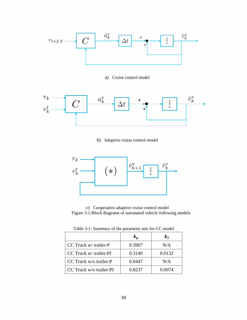
a) Cruise control model

b) Adaptive cruise control model

c) Cooperative adaptive cruise control model Figure 3-1:Block diagrams of automated vehicle following models

Table 3-1: Summary of the parameter sets for CC model

𝒌𝒌𝒑𝒑 𝒌𝒌𝑰𝑰

CC Truck w/ trailer-P 0.3907 N/A

CC Truck w/ trailer-PI 0.3140 0.0132

CC Truck w/o trailer-P 0.8447 N/A

CC Truck w/o trailer-PI 0.8237 0.0074

39

To validate the models, numerical simulations were carried out and results were compared with field test data. The performance summary of the model can be seen in Table 3-2. Mean speed error for these models varied between -0.0209 m/s and 0.0839 m/s, and RMSE ranged from 0.2938 m/s to 0.4231 m/s. In terms of Mean error and RMSE, both models simulated the real system very well and the maximum and the minimum error values were tolerable.

Comparing error values between two test scenarios, the error with trailer behind is higher than the error without trailer. This could be because the trailer introduces additional disturbances and nonlinearities, for example aero drag force and extra weight of the trailer, which cannot be represented completely by the linear model.

Table 3-2: CC model validation summary Duration

of Data [s]

Mean Error [m/s]

Max Error [m/s]

Min Error [m/s]

RMSE[m/s]

CC Truck w/ trailer-P 988.4 -0.0209 2.9130 -2.2995 0.4231

CC Truck w/ trailer-PI 988.4 0.0839 3.0098 -1.9770 0.4110

CC Truck w/o trailer-P 525.7 -0.0111 1.3744 -2.1290 0.2944

CC Truck w/o trailer-PI 525.7 0.0037 1.3726 -2.0707 0.2938

Figure 3-2 shows more details of the experiment data and outputs of the two models in the time domain. These figures display data for a portion of a much longer sample of test data. It should be noted that the CC data appear to be piecewise in these charts because the truck was traveling on a highway and due to slow traffic or lane changing maneuvers the truck driver had to deactivate CC. The CC data cover a range of speeds between 12.5 m/s to 24.4 m/s.

In general, the performance of both the P-model and PI-model are close to the field test data. However, in the case of truck with trailer, the PI-model tends to have overshoot. As a result, the P-model is better suited for modeling a truck with trailer to avoid overshoot, while the PI-model is suggested for modeling the truck without trailer, since it gives better RMSE than the other.

40

a) Truck with trailer

b) Truck without trailer Figure 3-2: Field test data compared to estimates based on P-model and PI-model for CC mode.

3.2.2 Adaptive cruise control driven truck ACC is a more sophisticated version of CC that adapts the vehicle speed based on the target vehicle speed and the target distance. In ACC, the subject vehicle follows the target vehicle at a fixed time gap which is selected by the driver.

The block diagram of the ACC car following is shown in Figure 3-1. There are two inputs, the target distance 𝑒𝑒𝑘𝑘, and the target vehicle speed 𝑣𝑣𝑘𝑘𝑡𝑡 ; and one output, which is an estimated subject vehicle speed 𝑣𝑣�𝑘𝑘𝑑𝑑. The cruise control model also consists of vehicle kinematics and

41

controller. The vehicle kinematics is the same as that in equation ( 3-2). The controller determines acceleration based on the target distance 𝑒𝑒𝑘𝑘 and the difference between the target vehicle speed 𝑣𝑣𝑘𝑘𝑡𝑡 and the subject vehicle speed 𝑣𝑣�𝑘𝑘𝑑𝑑. The controller equation is formulated in equation ( 3-8), which includes two terms. The first term is for tracking the driver’s desired time gap. The value in parenthesis is the gap error, which is the difference between real clearance gap 𝑒𝑒𝑘𝑘 and desired clearance gap 𝑡𝑡𝑡𝑡𝑣𝑣�𝑘𝑘𝑑𝑑. The desired time gap 𝑡𝑡𝑡𝑡 has been selected to be 1.5 seconds throughout the experiment. The second term is the speed error, which is the speed difference between the subject vehicle and the target vehicle.

𝑎𝑎�𝑘𝑘𝑑𝑑 = 𝑘𝑘1(𝑒𝑒𝑘𝑘 − 𝑡𝑡𝑡𝑡𝑣𝑣�𝑘𝑘𝑑𝑑) + 𝑘𝑘2 (𝑣𝑣𝑘𝑘𝑡𝑡 − 𝑣𝑣�𝑘𝑘𝑑𝑑) 3-8

The data fitting problem is formulated in equation ( 3-1) with prediction models which are formulated in ( 3-8) and ( 3-2). The input 𝑈𝑈𝑘𝑘 is [𝑒𝑒𝑘𝑘, 𝑣𝑣𝑘𝑘𝑡𝑡 ] and the unknown parameter θ is [k1, k2]. The optimal parameter values with and without a trailer are summarized in Table 3-3. Similar to the trend shown for the CC truck modelling, the gain for the ACC truck without trailer is larger than the gain with trailer, because the truck with trailer has a larger mass.

Validation results are summarized in Table 3-4. Mean error values are 0.0138 m/s and -0.0130 m/s for the truck with and without trailer, respectively. RMSE is 0.4676 m/s for the truck with trailer and 0.3041 m/s for the truck without trailer. The RMSE values are low and error values are bounded within tolerable range. This indicates the ACC model can properly predict field data.

Similar to the models developed for CC, the RMSE of the models of the truck with trailer is larger than that without trailer. This is also due to the additional disturbance and nonlinearity introduced by the trailer.

Table 3-3: Summary of the parameters for ACC model

k1 k2

ACC Truck w/ trailer 0.0561 0.3393

ACC Truck w/o trailer 0.1651 0.6371

Table 3-4: ACC model validation summary

Duration of Data [s]

Mean Error[m/s]

Max Error [m/s]

Min Error [m/s]

RMSE [m/s]

ACC Truck w/ trailer 726.3 0.0138 2.7681 -2.1681 0.4676

ACC Truck w/o trailer 1470.7 -0.0130 2.3546 -3.2687s 0.3041

42

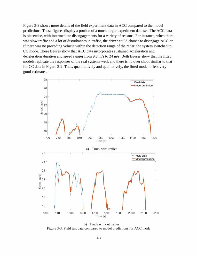
Figure 3-3 shows more details of the field experiment data in ACC compared to the model predictions. These figures display a portion of a much larger experiment data set. The ACC data is piecewise, with intermediate disengagements for a variety of reasons. For instance, when there was slow traffic and a lot of disturbances in traffic, the driver could choose to disengage ACC or if there was no preceding vehicle within the detection range of the radar, the system switched to CC mode. These figures show that ACC data incorporates sustained acceleration and deceleration duration and speed ranges from 9.8 m/s to 24 m/s. Both figures show that the fitted models replicate the responses of the real systems well, and there is no over shoot similar to that for CC data in Figure 3-2. Thus, quantitatively and qualitatively, the fitted model offers very good estimates.

a) Truck with trailer

b) Truck without trailer Figure 3-3: Field test data compared to model predictions for ACC mode

43

3.2.3 Cooperative adaptive cruise control driven truck Cooperative adaptive cruise control uses an on-board sensor to detect the immediately preceding vehicle plus wireless communication to receive additional information about multiple preceding vehicles. By using V2V communication, the response delay between the subject vehicle and the preceding vehicles can be reduced because the subject vehicle can start to brake and accelerate as soon as it receives messages about the actions of the preceding vehicles. The simplified model block diagram for use in traffic simulation is shown in Figure 3-1. This does not attempt to represent all the dynamic interactions among consecutive vehicles coupled together using CACC control, but only considers the approximate pairwise input-output relationships between consecutive CACC vehicles. It uses the target gap, the target vehicle speed, and the subject vehicle speed feedback as inputs to the controller. Detailed model equations are described below in equation ( 3-9).

𝑣𝑣�𝑘𝑘+1𝑑𝑑 = 𝑣𝑣�𝑘𝑘𝑑𝑑 + 𝑘𝑘𝑝𝑝𝑒𝑒𝑘𝑘 + 𝑘𝑘𝑑𝑑�̇�𝑒𝑘𝑘 3-9

where 𝑒𝑒𝑘𝑘 and �̇�𝑒𝑘𝑘 are defined as follows:

𝑒𝑒𝑘𝑘 = 𝑀𝑀𝑘𝑘𝑡𝑡 − 𝑀𝑀𝑘𝑘𝑑𝑑 − 𝑡𝑡𝑡𝑡𝑣𝑣𝑘𝑘𝑑𝑑 3-10 �̇�𝑒𝑘𝑘 = 𝑣𝑣𝑘𝑘𝑡𝑡 − 𝑣𝑣�𝑘𝑘𝑑𝑑 − 𝑡𝑡𝑡𝑡𝑎𝑎�𝑘𝑘𝑑𝑑 3-11

Since a vehicle is subject to kinematic relationships, the acceleration term 𝑎𝑎�𝑘𝑘𝑑𝑑 can be replaced by speed difference as the following equation shows.

𝑣𝑣�𝑘𝑘+1𝑑𝑑 = 𝑣𝑣�𝑘𝑘𝑑𝑑 + 𝑎𝑎�𝑘𝑘𝑑𝑑 Δ𝑡𝑡 ⇒ 𝑎𝑎�𝑘𝑘𝑑𝑑 = (𝑣𝑣�𝑘𝑘+1𝑑𝑑 − 𝑣𝑣�𝑘𝑘𝑑𝑑)/Δ𝑡𝑡 3-12

After discretizing equations ( 3-9 to 3-11) and substituting equation ( 3-12) into it, and manipulating the equation, the following equation can be obtained.

𝑣𝑣�𝑘𝑘+1𝑑𝑑 = 𝑣𝑣�𝑘𝑘𝑑𝑑 + 𝑘𝑘𝑝𝑝𝑒𝑒𝑘𝑘 + 𝑘𝑘𝑑𝑑(𝑣𝑣𝑘𝑘𝑡𝑡 − 𝑣𝑣�𝑘𝑘𝑑𝑑 − 𝑡𝑡ℎ𝑤𝑤(𝑣𝑣�𝑘𝑘+1𝑑𝑑 − 𝑣𝑣�𝑘𝑘𝑑𝑑)/Δ𝑡𝑡)

⇒ (1 + 𝑘𝑘𝑑𝑑𝑡𝑡ℎ𝑤𝑤/Δt )𝑣𝑣�𝑘𝑘+1𝑑𝑑 = (1 − 𝑘𝑘𝑑𝑑 + 𝑘𝑘𝑑𝑑𝑡𝑡ℎ𝑤𝑤/Δt) 𝑣𝑣�𝑘𝑘𝑑𝑑 + 𝑘𝑘𝑑𝑑𝑣𝑣𝑘𝑘𝑡𝑡 + 𝑘𝑘𝑝𝑝(𝑒𝑒𝑘𝑘 − 𝑡𝑡ℎ𝑤𝑤𝑣𝑣�𝑘𝑘𝑑𝑑) 3-13

The data fitting problem is formulated as equation ( 3-1) with the prediction model as formulated in equation ( 3-13). The input 𝑈𝑈𝑘𝑘 is [𝑒𝑒𝑘𝑘, 𝑣𝑣𝑘𝑘𝑡𝑡 ], and the unknown parameter θ is [𝑘𝑘𝑝𝑝,𝑘𝑘𝑑𝑑]. A typical numerical method to solve a convex problem starts with one initial value for each parameter 𝑘𝑘𝑝𝑝 and 𝑘𝑘𝑑𝑑 , and it iteratively improves the value of the parameters until it reaches the minimum mean square error. This approach may not work for this problem since the equation ( 3-13) is a nonlinear equality constraint, and the optimization formulation is not convex (33). As a result, the optimization solution may depend on the initial point from which the solution (or search) procedure starts. A typical approach to deal with this situation is to solve the problem for several different initial points and select the best solution. For this problem, we solved the problem 10

44

times and each time the initial point was randomly selected from the interval (0,1). The best optimum solution out of these ten solutions was then chosen.

In the CACC experiment, there were two CACC trucks following a leader in the CACC string. Models for truck 2 and truck 3 have been fitted separately because these trucks have different dynamic relationships to their predecessors. Truck 2 is only following truck 1, but truck 3 is responding to the motions of both trucks 1 and 2, so its response to truck 2 is inherently different from the response of truck 2 to the motions of truck 1.

Table 3-6 summarizes the statistics of the validation errors. Mean errors are equal to 0.0695 m/s and 0.0395 m/s for trucks 2 and 3, respectively. RMSE for truck 2 is equal to 0.2351 m/s and for truck 3 is equal to 0.4222 m/s. The mean error and the RMSE values are small, and the maximum and the minimum errors are within a tolerable range, which means the model can accurately simulate the CACC trucks.

Table 3-5: Summary of the parameter sets for CACC model

𝒌𝒌𝒑𝒑 𝒌𝒌𝒅𝒅

CACC Truck (Veh 2) 0.0074 0.0798

CACC Truck (Veh 3) 0.0034 0.0594

Table 3-6: CACC validation summary

Duration of Data

[s]

Mean Error[m/s]

Max Error[m/s]

Min Error [m/s]

RMSE(m/s)

CACC Truck (Veh 2) 1042.4 0.0695 2.5834 -0.9911 0.2351

CACC Truck (Veh 3) 857.3 0.0395 1.6250 -1.3560 0.4222

Figure 3-4 shows field data compared to model predictions for the trucks 2 and 3. The data cover speeds between 15 m/s and 28 m/s, and the trucks mostly follow the leader when their speed does not fluctuate drastically. The data show that when there was a significant speed reduction, the driver disengaged CACC. The plots show that model responses match the field test data very well, which means that the fitted model is reliable to use for microsimulation.

45

a) Truck 2

b) Truck 3 Figure 3-4: Field test data compared to model predictions for CACC mode

3.3 Conclusions Simple dynamic models have been defined to represent the performance of automatic car following systems, CC/ACC/CACC, for heavy trucks based on data from field experiments. The models for trucks with and without trailers are defined separately, since the dynamics of trucks with and without trailers vary significantly. The parameter identification for each given model structure is formulated as an optimization problem and solved numerically. After that, simulations were carried out to validate each model. Results show that the models match the real

46

system responses very well. Mean error values are small and errors are bounded within tolerable ranges for every model, so it should be possible to use these models with confidence to represent the performance of trucks with automatic car following capabilities in traffic microsimulations.

References 1) Nowakowski, C., Shladover, S. E., Lu, X. Y., Thompson, D., & Kailas, A. (2015). Cooperative adaptive cruise control (CACC) for truck platooning: Operational concept alternatives.

2) Arnaout, G. M., & Arnaout, J. P. (2014). Exploring the effects of cooperative adaptive cruise control on highway traffic flow using microscopic traffic simulation. Transportation Planning and Technology, 37(2), 186-199.

3) Kesting, A., Treiber, M., & Helbing, D. (2010). Enhanced intelligent driver model to access the impact of driving strategies on traffic capacity. Philosophical Transactions of the Royal Society of London A: Mathematical, Physical and Engineering Sciences, 368(1928), 4585-4605.

4) VanderWerf, J., Shladover, S., Miller, M., & Kourjanskaia, N. (2002). Effects of adaptive cruise control systems on highway traffic flow capacity. Transportation Research Record: Journal of the Transportation Research Board, (1800), 78-84.

5) Tsugawa, S., Jeschke, S., & Shladover, S. E. (2016). A review of truck platooning projects for energy savings. IEEE Transactions on Intelligent Vehicles, 1(1), 68-77.

6) Bonnet, Christophe, and Hans Fritz. Fuel consumption reduction in a platoon: Experimental results with two electronically coupled trucks at close spacing. No. 2000-01-3056. SAE Technical Paper, 2000.

7) Tsugawa S (2012) Energy ITS; What we learned and what we should learn. In: TRB road vehicle automation workshop, Irvine CA, 24–26 July 2012

8) Chan, Eric. "SARTRE automated platooning vehicles." Towards Innovative Freight and Logistics (2014): 137-150.

9) Lammert, M. P., Duran, A., Diez, J., Burton, K., & Nicholson, A. (2014). Effect of platooning on fuel consumption of class 8 vehicles over a range of speeds, following distances, and mass. SAE International Journal of Commercial Vehicles, 7(2014-01-2438), 626-639.

10) Roeth, M. "CR England Peloton Technology PlatooningTest ,Nov 2013." North American Council for Freight Efficiency (2013).

11) McAuliffe, Brian R.; Croken, Mark; Ahmadi-Baloutaki, Mojtaba; Raeesi, Arash, Fuel-Economy Testing of a Three-Vehicle Truck Platooning System, Report No.: LTR-AL-2017-0008

47

URL : http://nparc.cisti-icist.nrc-cnrc.gc.ca/eng/view/fulltext/?id=d21e1097-5d30-4a0f-b742-35ffad931c2f

12) Alam, A., Besselink, B., Turri, V., Martensson, J., & Johansson, K. H. (2015). Heavy-duty vehicle platooning for sustainable freight transportation: A cooperative method to enhance safety and efficiency. IEEE Control Systems, 35(6), 34-56.

13) Müller, S. (2012). The Impact of Electronic Coupled Heavy Trucks on Traffic Flow. ETC Proceedings.

14) Bibeka, A;, P. Songchitruksa, Y. Zhang, Assessing Environmental Impacts of Truck Platooning on Multilane Freeways, 96th Annual Meeting, . 2017, TRB Paper #17-03191,

15) Praharaj, A.; R. E. Turochy, D. M. Bevly, Modeling And Analysis Of Freeway Traffic Operations With Deployment Of Driver Assistive Truck Platooning Technology, 96th Annual Meeting, 2017, Paper 17-01643

16) Deng, Q. (2016). A general simulation framework for modeling and analysis of heavy-duty vehicle platooning. IEEE Transactions on Intelligent Transportation Systems, 17(11), 3252-3262.

17) Van Arem, B., Van Driel, C. J., & Visser, R. (2006). The impact of cooperative adaptive cruise control on traffic-flow characteristics. IEEE Transactions on Intelligent Transportation Systems, 7(4), 429-436.

18) Newell, G. F. (2002). A simplified car-following theory: a lower order model. Transportation Research Part B: Methodological, 36(3), 195-205.

19) Gipps, P. G. (1981). A behavioural car-following model for computer simulation. Transportation Research Part B: Methodological, 15(2), 105-111.

20) Lu, X. Y., Kan, X. D., Shladover, S. E., Wei, D., & Ferlis, R. A. (2017). An Enhanced Microscopic Traffic Simulation Model for Application to Connected Automated Vehicles, Presented at TRB 2017 (No. 17-05126).

21) Liu, H.; X. kan, S. E. Shladover, X. Lu, R. Ferlis, “Impact of Cooperative Adaptive Cruise Control (CACC) on 2 Multilane Freeway Merge Capacity”, Submitted to TRB 2018

22) Chou, F-C.; H. Ramezani, X. Lu, S. E. Shladover, “Modeling Vehicle-Following Dynamics of Heavy Trucks Under Automatic Speed Control Based on Experimental Data”, Submitted to TRB 2018 for presentation

23) Milanés, V., & Shladover, S. E. (2014). Modeling cooperative and autonomous adaptive cruise control dynamic responses using experimental data. Transportation Research Part C: Emerging Technologies, 48, 285-300.

48

24) Harwood, D. W. (2003). Review of truck characteristics as factors in roadway design (Vol. 505). Transportation Research Board.

25) Pline, J.L. (Ed.), 1999. Traffic Engineering Handbook -. 5th Edition. ITE, Institute of Transportation Engineers, Washington, DC.

26) Yang, S.; S. Shladover, X. Lu, H. Ramezani, K. Aravind, Investigating Drivers’ On-the-Road Experience of Using Cooperative Adaptive Cruise Control for Truck Platooning, submitted to TRB 2018.

27) Dowling, R., Skabardonis, A., & Alexiadis, V. (2004). Traffic analysis toolbox volume III: guidelines for applying traffic microsimulation modeling software (No. FHWA-HRT-04-040).

28) EPA webpage for MOVES, URL: https://www.epa.gov/moves

29) MOVES Technical Reports, Population and Activity of On-road Vehicles in MOVES2014, July 2015, EPA-420-D-15-001, URL: https://cfpub.epa.gov/si/si_public_file_download.cfm?p_download_id=527191

30) Giannelli, R. A., Nam, E. K., Helmer, K., Younglove, T., Scora, G., & Barth, M. (2005). Heavy-duty diesel vehicle fuel consumption modeling based on road load and power train parameters, No. 2005-01-3549. SAE Technical Paper.

31) L. Ljung, "System Identification," in Wiley Encyclopedia of Electrical and Electronics Engineering, ed: John Wiley & Sons, Inc., 2001.

32) Lu., X.-Y., and S.E. Shladover, “Integrated ACC and CACC Development for Heavy-Duty Truck Partial Automation”, American Control Conference, Seattle, WA, June 2017.

33) S. Boyd and L. Vandenberghe, Convex Optimization: Cambridge University Press, 2004.

49