Chapter 11

Microscopic Characterization of Nanofibers and Nanocrystals

Robert J. Moon*, Tiina Pöhler† and Tekla Tammelin†

*Forest ProductLaboratory, United States Forest Service, USA

†VTT, Espoo, Finland

Comprehensive characterization of cellulose nanomaterials (CNs) is needed to advance our understanding of these materials and enable material designers, models, and manu­facturers to make informed decisions in the development of new products and materials based on CNs. This chapter summarizes several characterization methods as they pertain to CNs, in particular to characterize CN morphology, structure, mechanical properties, and surface chemistry.

11.1. Introduction

There are variety of nanocellulose materials (CNs) that can be extracted by dif­ferent methods from a wide diversity of cellulose source materials (plant, tree, algae, bacteria, tunicate, etc.), both of which alter the resulting CN particle mor­phology, size distribution, degree of branching, percent crystallinity, crystal struc­ture, surface chemistry, etc. Characterization of CNs is not only needed to help differentiation between different CN types, but is needed to advance our under­standing of these materials and to give insight as to their role within suspensions or composite systems. With improved characterization of CN morphology, struc­ture, nanomechanical properties, and surface chemistry, it will provide the pos­sibility to understand processing-structureproperty relationships as it relates to CN particles themselves, CN-CN interactions, CN-liquid interactions, and CN­matrix interactions all of which are important for the design of improved rheological properties of suspensions, composite processing, composite design, and composite performance.

Several characterization techniques have been used to greatly expand our under­standing of the crystalline cellulose nanodomains within wood-based materials, pulps, and cellulose microfibrils. This provides valuable insight for CNs, as they are mostly made up of these nanodomains;however, one should be mindful that the CN extraction process produces particles that are different from these nanodomains, in

159

160 R. J. Moon, T. Pöhler and T . Tammelin

particular, their morphology, size, structure, and surface chemistry. This chapter summarizes several methods that have been shown to be particularly useful in nanoscale characterization of CN morphology, structure, mechanical properties, and surface chemistry.

11.2. Cellulose nanomaterials morphology characterization

A variety of measurement techniques have been used for characterizing CN mor­phology (length, width, aspect ratio) and their distributions. Each technique has certain advantages and disadvantages, some of which will be discussed.

11.2.1 Optical microscopy

The resolution of traditional optical microscopy does not extend to real nanoscale analysis. The theoretical resolution limit of optical microscopy is around 200 nm, and in practice, a common basic optical microscope has a resolution limit between 700 nm and 1 µm. Despite of this, optical microscopy can be used to illustrate the general CNs macroscale character, to show the tendency to form agglomerates and to determine the amount of macroscopic fraction.

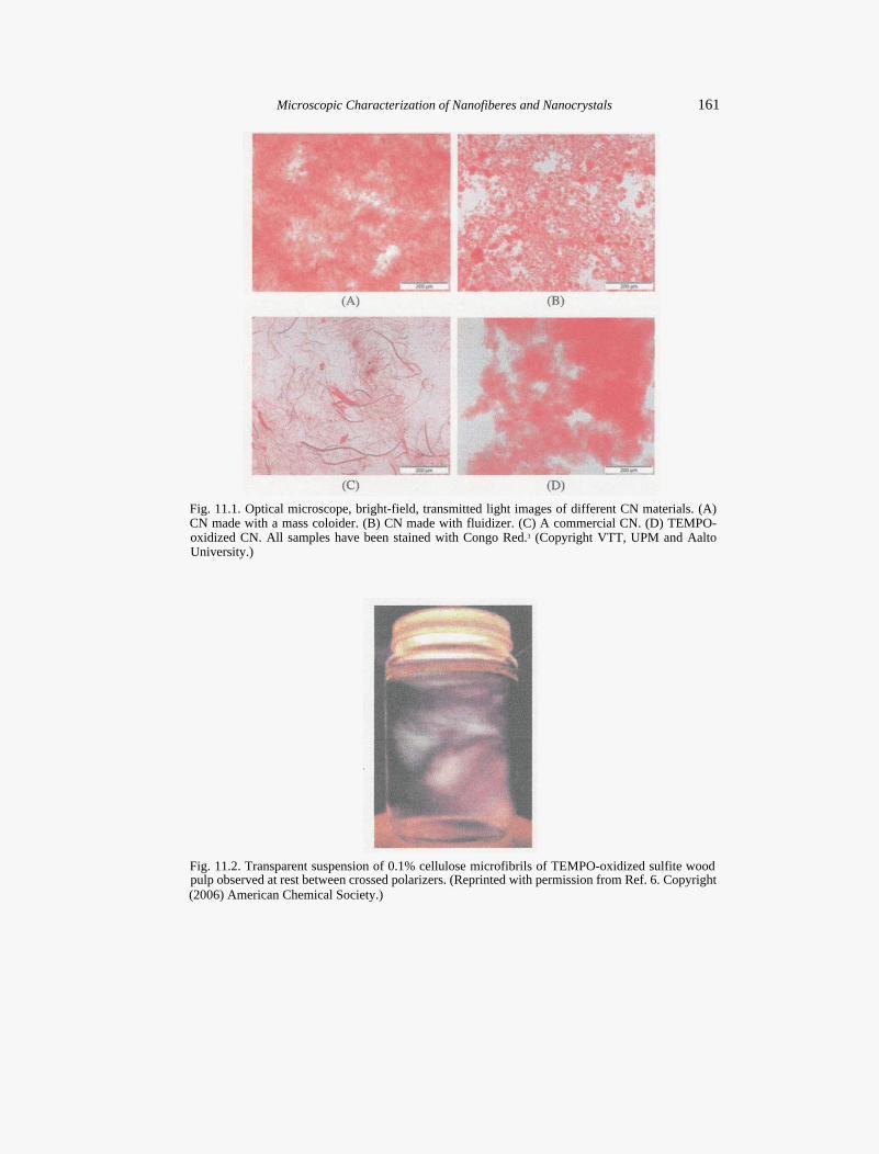
Bright-field microscopy is the simplest of all the optical microscopy illumination techniques. Sample is illuminated from below and observed from above. The contrast in the sample is caused by the absorbance of some of the light in the dense areas of the sample. Typically, bright-field microscopy has low contrast with most biological samples. Because of this, stains are often required for contrast enhancement. The most common stains for CNs are Congo Red and toluidine blue.1,2 Figure 11.1 shows bright-field optical microscope images of four different CNs. Clear differences in the amount of macroscopic, unfibrillated fiber fraction, and in the agglomeration of particles can be seen.

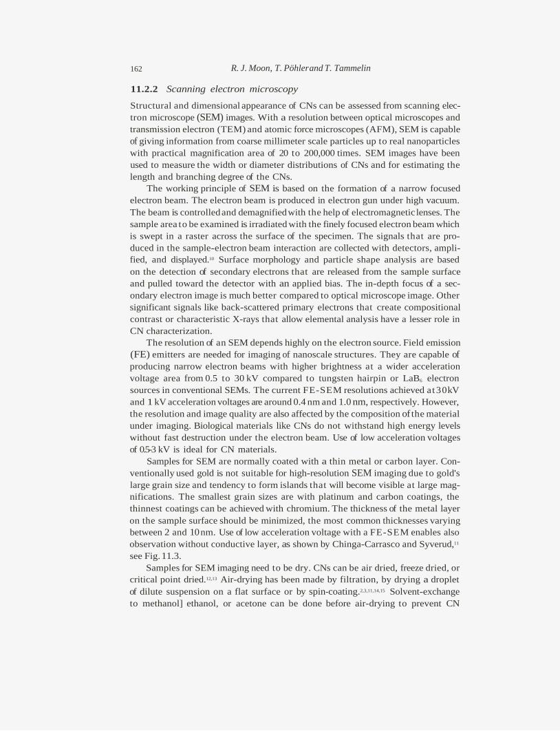
Another useful and commonly used contrast-enhancing technique is polarized light. It is used for observation and identification of birefringent materials. Polarized light responds to the molecular organization of biological samples, in particular crys­talline structures. This is true even though the organizing elements are far below the resolution of the light microscope.4 Cross-polarized light has been used to observe the macroscale progress of 2,2,6,6-tetramethylpiperidine-1-oxyl radical (TEMPO)­oxidation of cotton linter fibers as well as to indicate the success of nanoscale particle preparation in visually transparent solutions as shown in Fig. 11.2.5-7

Less frequently used optical technique is phase contrast microscopy that enhances the contrast of thin, transparent specimens without loss of resolution.8

Phase contrast is preferable to bright-field microscopy when high magnifications (up to 1000×) are needed and the specimen is colorless or the details so fine that color does not show up well. Phase contrast microscopy has been used to follow the swelling and fibrillation of TEMPO-oxidized cellulose fibers and in compar­ing the mechanical CN fibrillation methods and resulting CN branching degree in macroscale. 3,9

Microscopic Characterization of Nanofiberes and Nanocrystals 161

Fig. 11.1. Optical microscope, bright-field, transmitted light images of different CN materials. (A) CN made with a mass coloider. (B) CN made with fluidizer. (C) A commercial CN. (D) TEMPO-oxidized CN. All samples have been stained with Congo Red.3 (Copyright VTT, UPM and Aalto University.)

Fig. 11.2. Transparent suspension of 0.1% cellulose microfibrils of TEMPO-oxidized sulfite wood pulp observed at rest between crossed polarizers. (Reprinted with permission from Ref. 6. Copyright (2006) American Chemical Society.)

162 R. J. Moon, T. Pöhlerand T. Tammelin

11.2.2 Scanning electron microscopy

Structural and dimensional appearance of CNs can be assessed from scanning elec­tron microscope (SEM) images. With a resolution between optical microscopes and transmission electron (TEM) and atomic force microscopes (AFM), SEM is capable of giving information from coarse millimeter scale particles up to real nanoparticles with practical magnification area of 20 to 200,000 times. SEM images have been used to measure the width or diameter distributions of CNs and for estimating the length and branching degree of the CNs.

The working principle of SEM is based on the formation of a narrow focused electron beam. The electron beam is produced in electron gun under high vacuum. The beam is controlled and demagnified with the help of electromagnetic lenses. The sample area to be examined is irradiated with the finely focused electron beam which is swept in a raster across the surface of the specimen. The signals that are pro­duced in the sample-electron beam interaction are collected with detectors, ampli­fied, and displayed.10 Surface morphology and particle shape analysis are based on the detection of secondary electrons that are released from the sample surface and pulled toward the detector with an applied bias. The in-depth focus of a sec­ondary electron image is much better compared to optical microscope image. Other significant signals like back-scattered primary electrons that create compositional contrast or characteristic X-rays that allow elemental analysis have a lesser role in CN characterization.

The resolution of an SEM depends highly on the electron source. Field emission (FE) emitters are needed for imaging of nanoscale structures. They are capable of producing narrow electron beams with higher brightness at a wider acceleration voltage area from 0.5 to 30 kV compared to tungsten hairpin or LaB6 electron sources in conventional SEMs. The current FE-SEM resolutions achieved at 30kV and 1 kV acceleration voltages are around 0.4 nm and 1.0 nm, respectively. However, the resolution and image quality are also affected by the composition of the material under imaging. Biological materials like CNs do not withstand high energy levels without fast destruction under the electron beam. Use of low acceleration voltages of 0.5-3 kV is ideal for CN materials.

Samples for SEM are normally coated with a thin metal or carbon layer. Con­ventionally used gold is not suitable for high-resolution SEM imaging due to gold's large grain size and tendency to form islands that will become visible at large mag­nifications. The smallest grain sizes are with platinum and carbon coatings, the thinnest coatings can be achieved with chromium. The thickness of the metal layer on the sample surface should be minimized, the most common thicknesses varying between 2 and 10 nm. Use of low acceleration voltage with a FE-SEM enables also observation without conductive layer, as shown by Chinga-Carrasco and Syverud,11

see Fig. 11.3. Samples for SEM imaging need to be dry. CNs can be air dried, freeze dried, or

critical point dried.12,13 Air-drying has been made by filtration, by drying a droplet of dilute suspension on a flat surface or by spin-coating.2,3,11,14,15 Solvent-exchange to methanol] ethanol, or acetone can be done before air-drying to prevent CN

Microscopic Characterization of Nanofibers and Nanocrystals 163

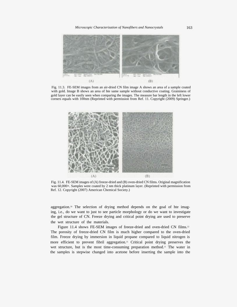
Fig. 11.3. FE-SEM images from an air-dried CN film image A shows an area of a sample coated with gold. Image B shows an area of hte same sample without conductive coating. Graininess of gold layer can be easily seen when comparing the images. The measure bar length in the left lower corners equals with 100nm (Reprinted with permission from Ref. 11. Copyright (2009) Springer.)

Fig. 11.4. FE-SEM images of (A) freeze-dried and (B) oven-dried CN films. Original magnification was 60,000×. Samples were coated by 2 nm thick platinum layer. (Reprinted with permission from Ref. 12. Copyright (2007) American Chemical Society.)

aggregation.16 The selection of drying method depends on the goal of hte imag­ing, i.e., do we want to just to see particle morphology or do we want to investigate the gel structure of CN. Freeze drying and critical point drying are used to preserve the wet structure of the materials.

Figure 11.4 shows FE-SEM images of freeze-dried and oven-dried CN films.12

The porosity of freeze-dried CN film is much higher compared to the oven-dried film. Freeze drying by immersion in liquid propane compared to liquid nitrogen is more efficient to prevent fibril aggregation.11 Critical point drying preserves the wet structure, but is the most time-consuming preparation method.11 The water in the samples is stepwise changed into acetone before inserting the sample into the

164 R. J. Moon, T. Pöhler and T. Tammelin

critical point dryer. The acetone is changed into liquid CO2 in the dryer and dried at supercritical point of CO2.

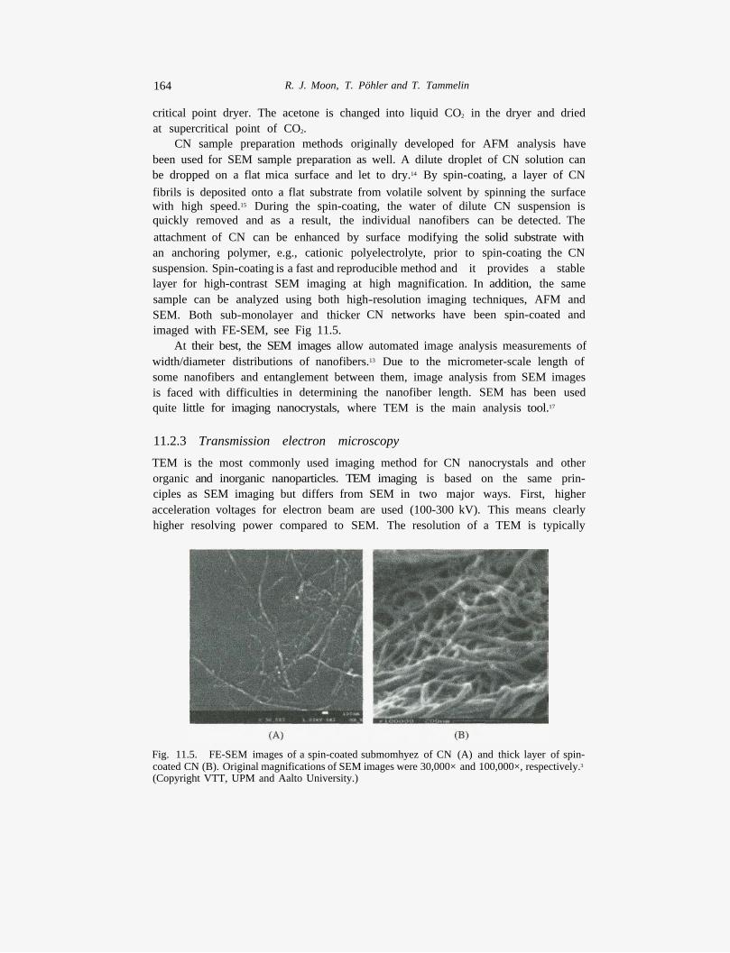
CN sample preparation methods originally developed for AFM analysis have been used for SEM sample preparation as well. A dilute droplet of CN solution can be dropped on a flat mica surface and let to dry.14 By spin-coating, a layer of CN fibrils is deposited onto a flat substrate from volatile solvent by spinning the surface with high speed.15 During the spin-coating, the water of dilute CN suspension is quickly removed and as a result, the individual nanofibers can be detected. The attachment of CN can be enhanced by surface modifying the solid substrate with an anchoring polymer, e.g., cationic polyelectrolyte, prior to spin-coating the CN suspension. Spin-coating is a fast and reproducible method and it provides a stable layer for high-contrast SEM imaging at high magnification. In addition, the same sample can be analyzed using both high-resolution imaging techniques, AFM and SEM. Both sub-monolayer and thicker CN networks have been spin-coated and imaged with FE-SEM, see Fig 11.5.

At their best, the SEM images allow automated image analysis measurements of width/diameter distributions of nanofibers.13 Due to the micrometer-scale length of some nanofibers and entanglement between them, image analysis from SEM images is faced with difficulties in determining the nanofiber length. SEM has been used quite little for imaging nanocrystals, where TEM is the main analysis tool.17

11.2.3 Transmission electron microscopy

TEM is the most commonly used imaging method for CN nanocrystals and other organic and inorganic nanoparticles. TEM imaging is based on the same prin­ciples as SEM imaging but differs from SEM in two major ways. First, higher acceleration voltages for electron beam are used (100-300 kV). This means clearly higher resolving power compared to SEM. The resolution of a TEM is typically

Fig. 11.5. FE-SEM images of a spin-coated submomhyez of CN (A) and thick layer of spin-coated CN (B). Original magnifications of SEM images were 30,000× and 100,000×, respectively.3

(Copyright VTT, UPM and Aalto University.)

Microscopic Characterization of nanofibers and Nanocrystals 165

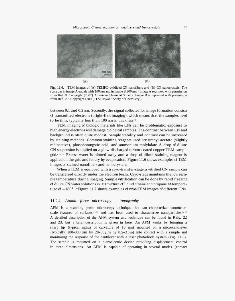
Fig. 11.6. TEM images of (A) TEMPO-oxidized CN nanofibers and (B) CN nanocrystals. The scale bar in image A equals with 100 nm and in image B 200 nm. (Image A reprinted with permission from Ref. 9. Copyright (2007) American Chemical Society. Image B is reprinted with permission from Ref. 20. Copyright (2008) The Royal Society of Chemistry.)

between 0.1 and 0.2 nm. Secondly, the signal collected for image formation consists of transmitted electrons (bright-fieldimaging), which means that the samples need to be thin, typically less than 100 nm in thickness.18

TEM imaging of biologic materials like CNs can be problematic: exposure to high energy electrons will damage biological samples. The contrast between CN and background is often quite modest. Sample stability and contrast can be increased by staining methods. Common staining reagents used are uranyl acetate (slightly radioactive), phosphotungstic acid, and ammonium molybdate. A drop of dilute CN suspension is applied on a glow-discharged carbon-coated copper TEM sample grid.9, 17, 19 Excess water is blotted away and a drop of dilute staining reagent is applied on the grid and let dry by evaporation. Figure 11.6 shows examples of TEM images of stained nanofibers and nanocrystals.

When a TEM is equipped with a cryo-transfer-stage, a vitrified CN sample can be transferred directly under the electron beam. Cryo-stage maintains the low sam­ple temperature during imaging. Sample vitrification can be done by rapid freezing of dilute CN water solutions in 1:1mixture of liquid ethane and propane at tempera­ture of -180°.2,14Figure 11.7 shows examples of cryo-TEM images of different CNs.

11.2-4 Atomic force microscopy – topography

AFM is a scanning probe microscopy technique that can characterize nanometer-scale features of surfaces,21-23 and has been used to characterize nanoparticles.24,25

A detailed description of the AFM system and technique can be found in Refs. 22 and 23, but a brief description is given in here. An AFM works by bringing a sharp tip (typical radius of curvature of 10 nm) mounted on a microcantilever (typically 200-300 µm by 20-35 µm by 0.5-3 µm) into contact with a sample and monitoring the response of the cantilever with a laser photodiode system (Fig. 11.8). The sample is mounted on a piezoelectric device providing displacement control in three dimensions. An AFM is capable of operating in several modes (contact

166 R. J. Moon, T. Pöhler and T. Tammelin

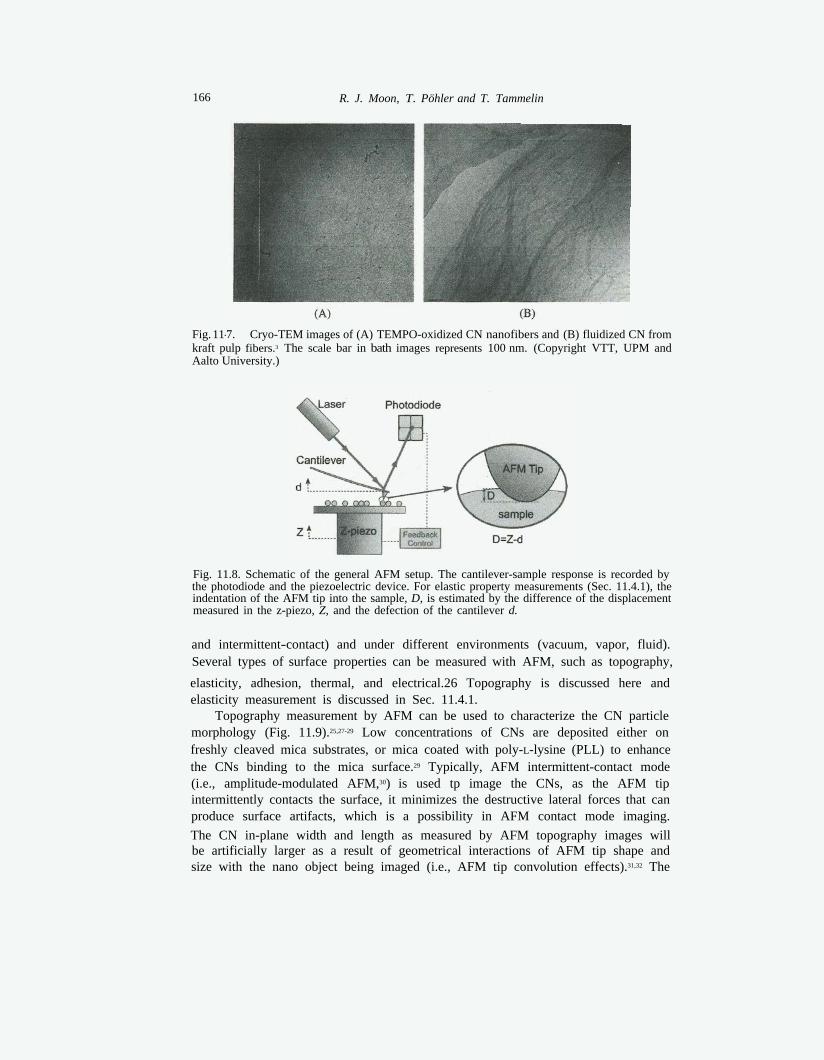
Fig. 11-7. Cryo-TEM images of (A) TEMPO-oxidized CN nanofibers and (B) fluidized CN from kraft pulp fibers.3 The scale bar in bath images represents 100 nm. (Copyright VTT, UPM and Aalto University.)

Fig. 11.8. Schematic of the general AFM setup. The cantilever-sample response is recorded by the photodiode and the piezoelectric device. For elastic property measurements (Sec. 11.4.1), the indentation of the AFM tip into the sample, D, is estimated by the difference of the displacement measured in the z-piezo, Z, and the defection of the cantilever d.

and intermittent-contact) and under different environments (vacuum, vapor, fluid). Several types of surface properties can be measured with AFM, such as topography,

elasticity, adhesion, thermal, and electrical.26 Topography is discussed here and elasticity measurement is discussed in Sec. 11.4.1.

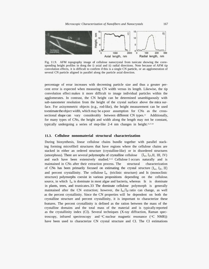
Topography measurement by AFM can be used to characterize the CN particle morphology (Fig. 11.9).25,27-29 Low concentrations of CNs are deposited either on freshly cleaved mica substrates, or mica coated with poly-L-lysine (PLL) to enhance the CNs binding to the mica surface.29 Typically, AFM intermittent-contact mode (i.e., amplitude-modulated AFM,30) is used tp image the CNs, as the AFM tip intermittently contacts the surface, it minimizes the destructive lateral forces that can produce surface artifacts, which is a possibility in AFM contact mode imaging. The CN in-plane width and length as measured by AFM topography images will be artificially larger as a result of geometrical interactions of AFM tip shape and size with the nano object being imaged (i.e., AFM tip convolution effects).31,32 The

Microscopic Characterization of Nanofibers and Nanocrystals 167

Fig. 11.9. AFM topography image of cellulose nanocrystal from tunicate showing the corre­sponding height profiles in dong the i) axial and ii) radial directions. Note because of AFM tip convolution effects, it is difficult to confirm if this is a single CN particle, or an agglomeration of several CN particle aligned in parallel along the particle axial direction.

percentage of errar increases with decreming particle size and thus a greater per­cent error is expected when measuring CN width versus its length. Likewise, the tip convolution effect makes it more difficult to image individual particles within the agglomerates. In contrast, the CN height can be determined unambiguously with sub-nanometer resolution from the height of the crystal surface above the mica sur­face. For axisymmetric objects (e.g., rod-like), the height measurement can be used toestimate the object width, which may be a poor assumption for CNs as the cross-sectional shape can vary considerably between different CN types.33 Additionally, for many types of CNs, the height and width along the length may not be constant, typically undergoing a series of step-like 2-4 nm changes in height.25,27,29

11.3. Cellulose nonomaterial structural characterization

During biosynthesis, linear cellulose chains bundle together with parallel stack­ing forming microfibril structures that have regions where the cellulose chains are stacked in either an ordered structure (crystalline-like) or in disordered structures (amorphous). There are several polymorphs of crystalline cellulose II, III, IV) and each have been extensively studied.33-35 Cellulose I occurs naturally and is maintained in CNs after their extraction process. The structural characterization of CNs has been primarily focused on estimating the crystal structure and percent crystallinity. The cellulose (triclinic structure) and Iß (monoclinic structure) polymorphs coexist in various propositions depending on the cellulose. source, in which is dominate in most algae and bacteria, whereas Iß is dominate in plants, trees, and trunicates.33 The dominate cellulose polymorph is generally maintained after the CN extraction; however, the ratio can change, as well as the percent crystallinity. Since the CN properties will be dependent on both the crystalline structure and percent crystallinity, it is important to characterize these features. The percent crystallinity is defined as the ration between the mass of the crystalline domains and the total mass of the material and is typically reported as the crystallinity index (CI). Several techniques (X-ray diffraction, Raman spec­troscopy, infrared spectroscopy and 13C nuclear magnetic resonance (13C NMR)) have been used to characterize CN crystal structure and CI. The CI estimations

168 R. J. Moon, T. Pöhler and T. Tammelin

will vary based on the technique used,36 differences in the data analysis,36,37 the quality of the peak deconvolution approaches,38,39 to name a few.

11.3.1 Wide-angle X-ray diffraction

Wide-angle X-ray diffraction (WAXD) measures the diffracting X-rays of a given sample (usually fine powdered materials with randomly oriented particles) as a function of the diffraction angle (26) with respect to the direction of the primary X-ray beam (e.g., monochromatic X-ray, = 0.1541 nm, from radiation gen­erated at a given accelerating voltage and current). Diffracting X-rays occur only at specific conditions based upon the internal structure of the solid, which can be used to assess crystal structure and percent crystallinity. For cellulose I, diffrac­tion peaks are at 26 of ~14.5°, ~16.6°, ~20.4°, ~22.7°, and ~34.4°, correspond­

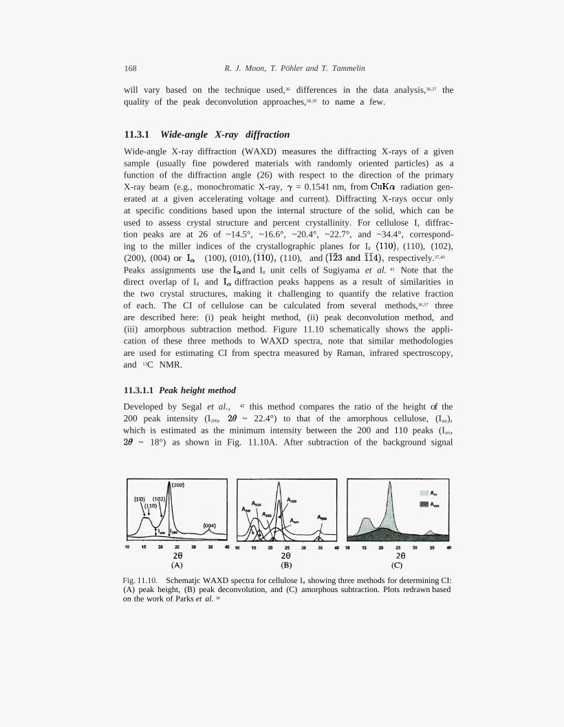
(110), (102), (200), (004) or (100), (010), (110), and Peaks assignments use the and Iß unit cells of Sugiyama et al. 41 Note that the direct overlap of Iß and diffraction peaks happens as a result of similarities in the two crystal structures, making it challenging to quantify the relative fraction of each. The CI of cellulose can be calculated from several methods,36,37 three are described here: (i) peak height method, (ii) peak deconvolution method, and (iii) amorphous subtraction method. Figure 11.10 schematically shows the appli­cation of these three methods to WAXD spectra, note that similar methodologies are used for estimating CI from spectra measured by Raman, infrared spectroscopy, and 13C NMR.

ing to the miller indices of the crystallographic planes for Iß

respectively.37,40

11.3.1.1 Peak height method

Developed by Segal et al., 42 this method compares the ratio of the height of the 200 peak intensity (I200, ~ 22.4°) to that of the amorphous cellulose, (Iam), which is estimated as the minimum intensity between the 200 and 110 peaks (Iam,

~ 18°) as shown in Fig. 11.10A. After subtraction of the background signal

Fig. 11.10. Schematjc WAXD spectra for cellulose Iß showing three methods for determining CI: (A) peak height, (B) peak deconvolution, and (C) amorphous subtraction. Plots redrawn based on the work of Parks et al. 36

Microscopic Characterization of Nanofibers and Nanocrystals 169

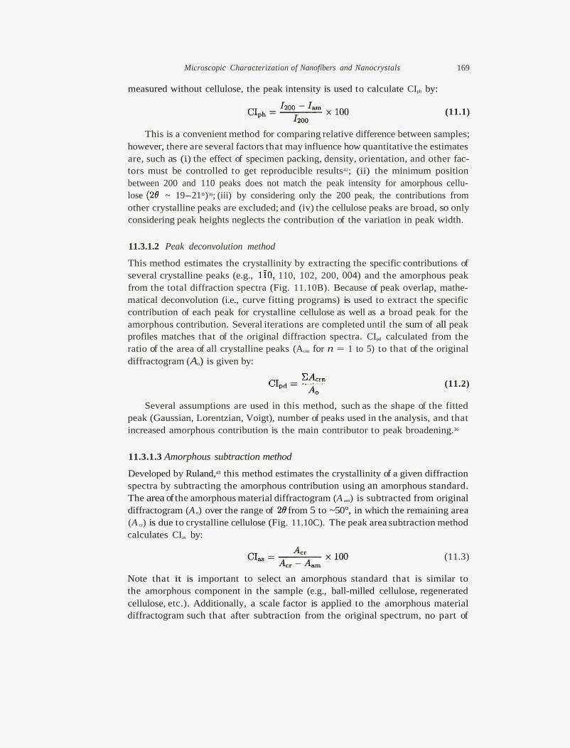
measured without cellulose, the peak intensity is used to calculate CIph by:

(11.1)

This is a convenient method for comparing relative difference between samples; however, there are several factors that may influence how quantitative the estimates are, such as (i) the effect of specimen packing, density, orientation, and other fac­tors must be controlled to get reproducible results42; (ii) the minimum position between 200 and 110 peaks does not match the peak intensity for amorphous cellu­lose ~ 19-21°)36; (iii) by considering only the 200 peak, the contributions from other crystalline peaks are excluded; and (iv) the cellulose peaks are broad, so only considering peak heights neglects the contribution of the variation in peak width.

11.3.1.2 Peak deconvolution method

This method estimates the crystallinity by extracting the specific contributions of several crystalline peaks (e.g., 110, 102, 200, 004) and the amorphous peak from the total diffraction spectra (Fig. 11.10B). Because of peak overlap, mathe­matical deconvolution (i.e., curve fitting programs) is used to extract the specific contribution of each peak for crystalline cellulose as well as a broad peak for the amorphous contribution. Several iterations are completed until the sum of all peak profiles matches that of the original diffraction spectra. CIpd calculated from the ratio of the area of all crystalline peaks (Acrn for n = 1 to 5) to that of the original diffractogram (Ao) is given by:

(11.2)

Several assumptions are used in this method, such as the shape of the fitted peak (Gaussian, Lorentzian, Voigt), number of peaks used in the analysis, and that increased amorphous contribution is the main contributor to peak broadening.36

11.3.1.3 Amorphous subtraction method

Developed by Ruland,43 this method estimates the crystallinity of a given diffraction spectra by subtracting the amorphous contribution using an amorphous standard. The area of the amorphous material diffractogram (A am) is subtracted from original diffractogram (A o) over the range of from 5 to ~50°, in which the remaining area (A cr) is due to crystalline cellulose (Fig. 11.10C). The peak area subtraction method calculates CIas by:

(11.3)

Note that it is important to select an amorphous standard that is similar to the amorphous component in the sample (e.g., ball-milled cellulose, regenerated cellulose, etc.). Additionally, a scale factor is applied to the amorphous material diffractogram such that after subtraction from the original spectrum, no part of

170 R. J. Moon, T. Pöhler and T. Tammelin

the residual spectrum (i.e., over the range of from 5 to 50°) contains a negative signal.36,37

11.3.2 Raman spectroscopy

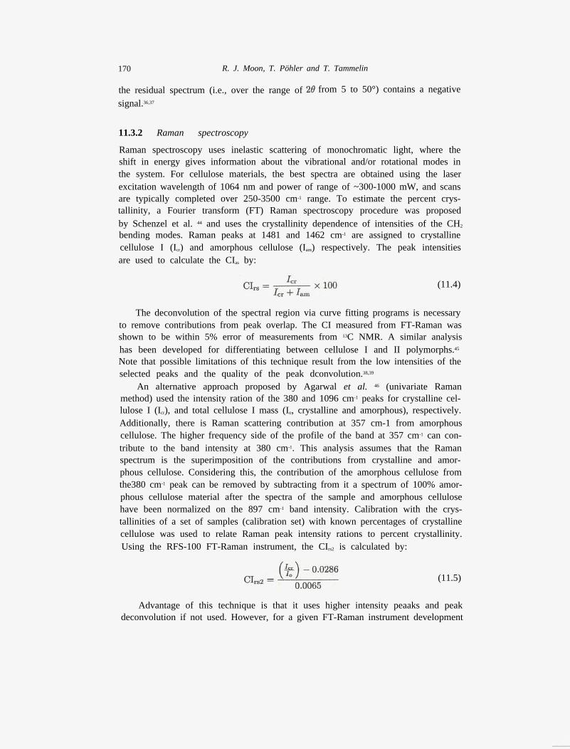
Raman spectroscopy uses inelastic scattering of monochromatic light, where the shift in energy gives information about the vibrational and/or rotational modes in the system. For cellulose materials, the best spectra are obtained using the laser excitation wavelength of 1064 nm and power of range of ~300-1000 mW, and scans are typically completed over 250-3500 cm-1 range. To estimate the percent crys­tallinity, a Fourier transform (FT) Raman spectroscopy procedure was proposed by Schenzel et al. 44 and uses the crystallinity dependence of intensities of the CH2

bending modes. Raman peaks at 1481 and 1462 cm-1 are assigned to crystalline cellulose I (Icr) and amorphous cellulose (Iam) respectively. The peak intensities are used to calculate the CIas by:

(11.4)

The deconvolution of the spectral region via curve fitting programs is necessary to remove contributions from peak overlap. The CI measured from FT-Raman was shown to be within 5% error of measurements from 13C NMR. A similar analysis has been developed for differentiating between cellulose I and II polymorphs.45

Note that possible limitations of this technique result from the low intensities of the selected peaks and the quality of the peak dconvolution.38,39

An alternative approach proposed by Agarwal et al. 46 (univariate Raman method) used the intensity ration of the 380 and 1096 cm-1 peaks for crystalline cel­lulose I (Icr), and total cellulose I mass (Io, crystalline and amorphous), respectively. Additionally, there is Raman scattering contribution at 357 cm-1 from amorphous cellulose. The higher frequency side of the profile of the band at 357 cm-1 can con­tribute to the band intensity at 380 cm-1. This analysis assumes that the Raman spectrum is the superimposition of the contributions from crystalline and amor­phous cellulose. Considering this, the contribution of the amorphous cellulose from the380 cm-1 peak can be removed by subtracting from it a spectrum of 100% amor­phous cellulose material after the spectra of the sample and amorphous cellulose have been normalized on the 897 cm-1 band intensity. Calibration with the crys­tallinities of a set of samples (calibration set) with known percentages of crystalline cellulose was used to relate Raman peak intensity rations to percent crystallinity. Using the RFS-100 FT-Raman instrument, the CIrs2 is calculated by:

(11.5)

Advantage of this technique is that it uses higher intensity peaaks and peak deconvolution if not used. However, for a given FT-Raman instrument development

Microscopic Characterization of Nanofibers and Nanocrystals 171

of a calibration curve relating the Raman peak intensity ratios to percent crystallini­ties (of calibration set samples) is necessary. Moreover, it is worth noting that com­pared to the crystallinities obtained by the Segal peak height method, the Raman estimates were significantlylower. The latter is due to the fact that the calibration set crystallinities were based on the lower WAXD crystallinity (compared to Segal peak height value) of the highly crystalline Whatman CC31 cellulose sample that was calculated after the amorphous contribution was subtracted at 21°

11.3.3 Fourier transform infrared spectroscopy

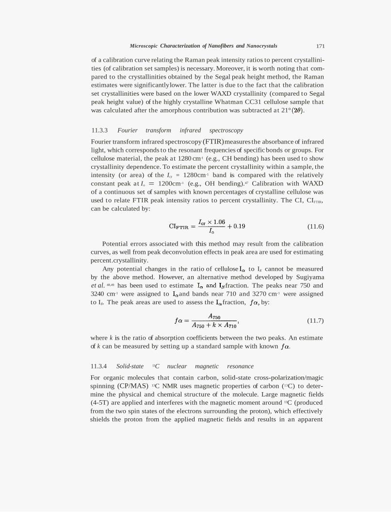
Fourier transform infrared spectroscopy (FTIR)measures the absorbance of infrared light, which corresponds to the resonant frequencies of specific bonds or groups. For cellulose material, the peak at 1280 cm-1 (e.g., CH bending) has been used to show crystallinity dependence. To estimate the percent crystallinity within a sample, the intensity (or area) of the Icr = 1280cm-1 band is compared with the relatively constant peak at Io = 1200cm-1 (e.g., OH bending).47 Calibration with WAXD of a continuous set of samples with known percentages of crystalline cellulose was used to relate FTIR peak intensity ratios to percent crystallinity. The CI, CIFTIR, can be calculated by:

(11.6)

Potential errors associated with this method may result from the calibration curves, as well from peak deconvolution effects in peak area are used for estimating percent.crystallinity.

Any potential changes in the ratio of cellulose to Iß cannot be measured by the above method. However, an alternative method developed by Sugiyama et al. 48,49 has been used to estimate fraction. The peaks near 750 and 3240 cm-1 were assigned to and bands near 710 and 3270 cm-1 were assigned to Iß. The peak areas are used to assess the fraction, by:

(11.7)

where k is the ratio of absorption coefficients between the two peaks. An estimate of k can be measured by setting up a standard sample with known

11.3.4 Solid-state l3C nuclear magnetic resonance

For organic molecules that contain carbon, solid-state cross-polarization/magic spinning (CP/MAS) 13C NMR uses magnetic properties of carbon (13C) to deter­mine the physical and chemical structure of the molecule. Large magnetic fields (4-5T) are applied and interferes with the magnetic moment around 13C (produced from the two spin states of the electrons surrounding the proton), which effectively shields the proton from the applied magnetic fields and results in an apparent

172 R. J. Moon T. Pöhler and T. Tammelin

adsorption of energy. The magnetic moment around 13C is dependent on the cova­ lent bonding and small changes in the energy sbsorption (as measured in parts per million, ppm) can be used to estimate the physical and chemical structure of the given molecule.

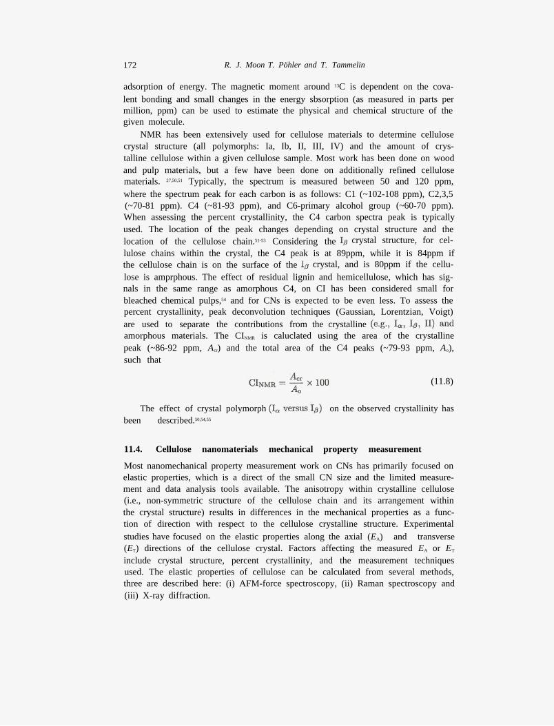
NMR has been extensively used for cellulose materials to determine cellulose crystal structure (all polymorphs: Ia, Ib, II, III, IV) and the amount of crys­talline cellulose within a given cellulose sample. Most work has been done on wood and pulp materials, but a few have been done on additionally refined cellulose materials. 27,50,51 Typically, the spectrum is measured between 50 and 120 ppm, where the spectrum peak for each carbon is as follows: C1 (~102-108 ppm), C2,3,5 (~70-81 ppm). C4 (~81-93 ppm), and C6-primary alcohol group (~60-70 ppm). When assessing the percent crystallinity, the C4 carbon spectra peak is typically used. The location of the peak changes depending on crystal structure and the location of the cellulose chain.51-53 Considering the crystal structure, for cel­lulose chains within the crystal, the C4 peak is at 89ppm, while it is 84ppm if the cellulose chain is on the surface of the crystal, and is 80ppm if the cellu­lose is amprphous. The effect of residual lignin and hemicellulose, which has sig­nals in the same range as amorphous C4, on CI has been considered small for bleached chemical pulps,54 and for CNs is expected to be even less. To assess the

are used to separate the contributions from the crystalline amorphous materials. The CINMR is caluclated using the area of the crystalline peak (~86-92 ppm, Acr) and the total area of the C4 peaks (~79-93 ppm, Ao), such that

percent crystallinity, peak deconvolution techniques (Gaussian, Lorentzian, Voigt)

(11.8)

The effect of crystal polymorph on the observed crystallinity has been described.50,54,55

11.4. Cellulose nanomaterials mechanical property measurement

Most nanomechanical property measurement work on CNs has primarily focused on elastic properties, which is a direct of the small CN size and the limited measure­ment and data analysis tools available. The anisotropy within crystalline cellulose (i.e., non-symmetric structure of the cellulose chain and its arrangement within the crystal structure) results in differences in the mechanical properties as a func­tion of direction with respect to the cellulose crystalline structure. Experimental studies have focused on the elastic properties along the axial (EA) and transverse (ET) directions of the cellulose crystal. Factors affecting the measured EA or ET

include crystal structure, percent crystallinity, and the measurement techniques used. The elastic properties of cellulose can be calculated from several methods, three are described here: (i) AFM-force spectroscopy, (ii) Raman spectroscopy and (iii) X-ray diffraction.

Microscopic Characterization of Nanofibers and Nanocrystals 173

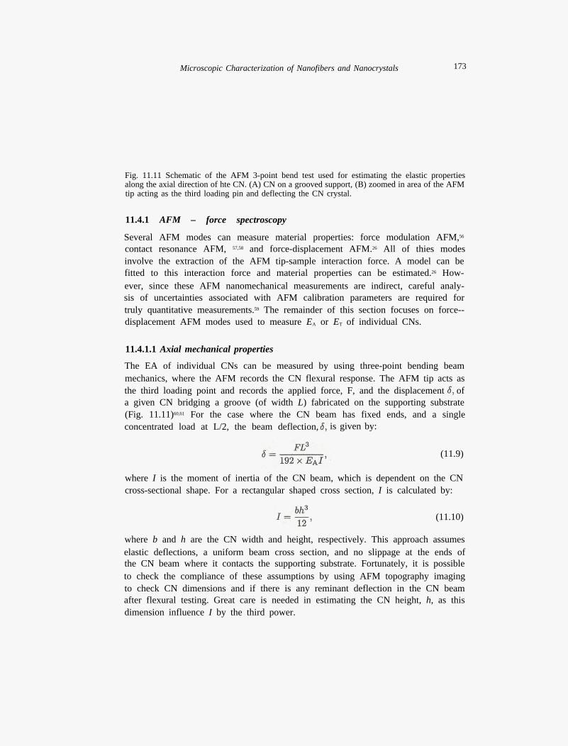
Fig. 11.11 Schematic of the AFM 3-point bend test used for estimating the elastic properties along the axial direction of hte CN. (A) CN on a grooved support, (B) zoomed in area of the AFM tip acting as the third loading pin and deflecting the CN crystal.

11.4.1 AFM – force spectroscopy

Several AFM modes can measure material properties: force modulation AFM,56

contact resonance AFM, 57,58 and force-displacement AFM.26 All of thies modes involve the extraction of the AFM tip-sample interaction force. A model can be fitted to this interaction force and material properties can be estimated.26 How­ever, since these AFM nanomechanical measurements are indirect, careful analy­sis of uncertainties associated with AFM calibration parameters are required for truly quantitative measurements.59 The remainder of this section focuses on force--displacement AFM modes used to measure EA or ET of individual CNs.

11.4.1.1 Axial mechanical properties

The EA of individual CNs can be measured by using three-point bending beam mechanics, where the AFM records the CN flexural response. The AFM tip acts as the third loading point and records the applied force, F, and the displacement of a given CN bridging a groove (of width L) fabricated on the supporting substrate (Fig. 11.11)60,61 For the case where the CN beam has fixed ends, and a single concentrated load at L/2, the beam deflection, is given by:

(11.9)

where I is the moment of inertia of the CN beam, which is dependent on the CN cross-sectional shape. For a rectangular shaped cross section, I is calculated by:

(11.10)

where b and h are the CN width and height, respectively. This approach assumes elastic deflections, a uniform beam cross section, and no slippage at the ends of the CN beam where it contacts the supporting substrate. Fortunately, it is possible to check the compliance of these assumptions by using AFM topography imaging to check CN dimensions and if there is any reminant deflection in the CN beam after flexural testing. Great care is needed in estimating the CN height, h, as this dimension influence I by the third power.

174 R. J. Moon, T. Pöhler and T. Tammelin

11.4.1.2 Transverse mechanical properties

The ET of individual CNs can be measured by nanoscale indentation of the AFM tip into the CN surface via AFM force-displacement mode (F-2 AFM).25,29,59,62

The process to do this is well established26 and can be summarized in three steps: (i) calibration of the AFM system, (ii) conversion to produce F-D curves, (iii) model fitting for the material property eatmation. The basic F-2 AFM experiment con­sists of bringing the AFM tip into contact with the sample, indenting the tip into the sample, and retracting the tip from the sample using the Z-piezo (e.g., z-direction piezoelectric actuator). The calibration parameters are needed to con­vert the raw data outputs that are in voltages from photodiode (movement of the cantilever) and the Z-piezo into forces, F, and displacements, Z, respectively, The resulting F-Z data is then converted into a force versus tip-sample distance (F-D) curve by subtracting the cantilever deflection from the Z-piezo position (Fig. 11.8). Note that the F-D curve differs from the F-2 curve in that the tip-slanaple gap (i.e., indentation depth) is the independent variable, whereas in the F-Z curve, the Z-piezo pesition is the independent variable. The resulting F-D curve is fit to a mathematical model (JKR,63 DMT64) that contains relevant system proper­ties (contact geometry, indenter tip shape and radius, elastic modulus of tip and sample, surface adhesion, etc.), from which the desired mechanical property can be extracted. Several classes of models can describe the interaction of an AFM tip with a surface, such as molecular dynamics simulations, finite element mod­els, and continuum analytical contact. This approach for estimating ET has many assumptions (smooth surfaces, semi-infinite mediums, isotropic material behavior, no edge effects, etc.) and large uncertainties in the calibrations and conversion of F-Z to F-D data, suggesting be challenging.59

11.4.2 Raman spectroscopy

Raman spectroscopy can be used to measure EA of CNs, in which in situ experi­ments usisng CN-polymer matrix composites are loaded in tension (tensile test or in bending) while simultaneoulsy evaluated via Raman.65-67 Shifts in the charac­teristic Raman peak for cellulose I (1095 cm-1) monitors strain along the axial direction of the crystals. The micron-sized laser spot size samples several CNs within a single measurement, giving an averaged strain and thus an average value for EA. Errors associated with this technique likely manifest from the assumed perfect CN-matrix load transfer and assumed two-dimensional CN network (as compared to one or three dimensional), both of which will be strongly depend­ing on how the CN composite is produced. It is worth noting that this Raman technique has been used to investigate CN-CN and CN-matrix load transfer effi­ciency by studying the changes in the amount of induced CN strain for a given applied tenile force to the composite, as a function of CN surface functionaliza­tion, the presence of water, and heating the nanocomposite above the glass transi­tion temperature.68

Microscopic Characterization of Nanofibers and Nanocrystals 175

11.4.3 X-ray diffraction and inelastic X-ray scattering

X-ray diffraction techniques have been used to measure EA of cellulose I crys­talline regions within cellulose microfibril bundles. One approach uses bulk-sized specimens consisting of parallel aligned cellulose microfibrils bundles (typically flax fibers) loaded along the fibril axis direction and X-ray diffraction is used to measure the small axial strains in the crystalline cellulose domains, which is subsequently used to calculate EA.69 This technique assumes perfect load transfer and perfect orientation of the cellulose crystals within the microfibril along the axis of load­ing, which are unlikely and will result in an underestimation of EA. An alternative approach uses inelastic X-ray scattering (IXS) of cellulose microfibrils and mea­sures the sound velocity as a function of acoustic phonon dispersion through the crystalline regions.70 This technique avoids the perfect load transfer issues described for the X-ray diffraction approach above, and can measure both EA and ET. One should use caution in applying these measured properties to CNs. Even though CNs can be considered to be the extracted crystalline regions within cellulose microfib­rils, the influence of the particle extraction process and increased surface area needs to be accounted for.

11.5. Cellulose nanomaterials surface chemistry

The CN surface chemistry will dictate how the CN interacts with its environment (CN-CN, CN-liquid interactions, CN-matrix, etc.), which subsequently effects rhe­ological properties in suspensions and load transfer in composites. To gain insight into CN surfaces is important to quantify exposed functional groups, uniformity of coverage, and location of the functionalization; however, it is extremely difficult to do such measurements. It is beyond the scope of this chapter to discuss details of specific techniques for surface characterization, but a literature review by Gardner et al. 71 summarizes the surface chemistry measurements of cellulose-based materi­als, including thin films, fibers, microcrystalline cellulose, and CNs. For CNs, it is plausible that AFM, FT-Raman, FT-IR, and 13C NMR could be used to help iden­tify modification-specific sites on CN surfaces. AFM adhesion maps have already been completed on individual CNS,25,72 it may be possible to use AFM chemical force microscopy,73 which uses chemically modified AFM tips, to study the range of specific chemical interactions with a given CN surface to produce interaction potential maps as a function of location. Likewise, a recent FT-Raman study by Agarwal e t a l 74 showed evidence for acetylation being restricted to CN surfaces based on the appearance of a band at 2938 cm-1 and the observation that the CN crystallinity did not decline upon acetylation.

Additionally, in situ surface characterization offers the additional capability of monitoring changes of an individual CN surface chemistry as a direct result of changes in the environment. Surface chemistry and functionalization have been investigated for microcrystalline cellulose75 and cellulose fibers using imaging tech­niques that employ the labeling of target molecules that then chemically bond to specific sites on a given surface. Labeling by organic dyes, semiconductor quantum

176 R. J. Moon, T. Pöhler and T. Tammelin

dots, and fluorescent proteins has been used, and these have been imaged using fluorescence spectroscopy, AFM, and TEM. These techniques provide a visual map of the surface chemistry and qualitative concentrations.

11.6. Conclusions

This chapter summarizes several of the more prevalent methods used to date to characterize CN particle morphology (optical microscopy, SEM, TEM, AFM), struc­ture (WAXD, Raman, FTIR, NMR), mechanical properties (AFM, Raman, WAXD, IXS), and surface chemistry (AFM). For several of these characterization methods, the small size and high surface area of CN particles result in some unique challenges for quantitative measurements and require special attention as briefly described. Progress is being made for improved characterization of CNs, and with this our understanding of these materials is also growing.

References 1. T. Saito, M. Hirota, N. Tamura, S. Kimura, H. Fukuzumi, L. Heux and A. Isogai,

Individualization of nano-sized plant cellulose fibrils by direct surface carboxylationusing TEMPO catalyst under neutral conditions, Biomacromolecules 10(7) (2009)1992-1996.

2. J. Vartiainen, T. Pöhler, K. Sirola, L. Pylkkänen, H. Alenius, J. Hokkinen, U. Tapper,P. Lahtinen, A. Kapanen, K. Putkisto, P. Hiekkataipale, P. Eronen, J. Ruokolainenand A. Laukkanen, Health and environmental safety aspects of friction grinding andspray drying of microfibrillated cellulose, Cellulose 18 (2011) 775-786.

3. T. Pöhler, T. Lappalainen, T. Tammelin, P. Eronen, P. Hiekkataipale, A. Vehniäinenand T.M. Koskinen, Influence of fibrillation method on the character of nanofibril­lated cellulose (NFC). [Network document]. Proceedings of 2010 TAPPI internationalconference on nanotechnology for the forest product industry, Espoo, Finland (2010).Available at http://www.tappi.org/content/events/10nano/papers/8.2.pdf

4. P. Whittaker, M.E. Schwab and P.B. Canham, The molecular organization of collagenin saccular aneurysms assessed by polarized light microscopy, Connect Tissue Res.17(1) (1988) 43-54.

5. T. Saito and A. Isogai, TEMPO-mediated oxidation of native cellulose. The effect ofoxidation conditions on chemical and crystal structures of the water-insoluble fractions,Biomacromolecules 5 (2004) 1983-1989.

6. T. Saito, Y. Nishiyama, J.-L. Putaux, M. Vignon and A. Isogai, Homogeneous suspen­sions of individualized microfibrils from TEMPO-catalyzed oxidation of native cellu­lose, Biomacmmolecules 7 (2006) 1687-1691,

7. I. Kvien, J. Sugiyama, M. Votrubec and K. Oksman, Characterization of starch basednanocomposites, J. Mater. Sci. 42 (19) (2007) 8163-8171.

8. L. Robertson, The use of phase-contrast microscopy to assess and differentiate themicrobial population of a paper mill, TAPPI J. 76(3) (1992), 83-87.

9. T. Saito, S. Kimura, Y. Nishiyama and A. Isogai, Cellulose nanofibers preparedby TEMPO-mediated oxidation of native cellulose, Biomacromolecules 8(8) (2007)2485-2491.

10. J.I. Goldstein, D.E. Newbury, P. Echlin, D.C. Joy, A.D. Romig, Jr. C.E. Lyman,C. Fiori and E. Lifshin, Scanning Electron Microscopy and X-ray Microanalysis. AText for Biologists, Material Scientists, and Geologists, 2nd edn., New York: PlenumPress(1992).

Microscopic Characterization of Nanofibers and Nanocrystals 177

11. G. Chinga-Carrasco and K. Syverud, Computer-misted quantification of the multi­scale films made of nanofibrillated cellulose, J. Nanopart Res. 12(3) (2010) 841-851.

12. J.T. Korhonen, P. Hiekkataipale, J. Malm, M. Karppinen, 0. Ikkala and R.H.A. Ras,Inorganic hollow nanotube aerogels by atomic layer deposition onto native nanocellu­lose templates, ACS Nano 5(3) (2011) 1967-1974.

13. K. Abe, S. Iwamoto and H. Yano, Obtaining cellulose nanofibers with a uniform widthof 15 nm from wood, Biomacromolecules 8(10) (2007) 3276-3278.

14. M. Pääkkö, M. Ankerfors, H. Kosonen, A. Nykänen, S. Ahola, M. Österberg, J. Ruoko­lainen, J. Laine, P.T. Larsson, O. Ikkala and T. Lindström, Enzymatic hydrolysiscombined with mechanical shearing and high-pressure homogenization for nanoscalecellulose fibrils and strong gels, Biomacromolecules 8(6) (2007) 1934-1941.

15. S. Ahola, J. Salmi, L.-S. Johansson, J. Laine and M. Österberg, Model films fromnative cellulose nanofibrils. Preparation, swelling, and surface interactions, Biomacro­molecules 9(4) (2008) 1273-1282.

16. M. Henriksson, L.A. Berglund, P. Isaksson, T. Lindström and T. Nishino, Cellulosenanopaper structures of high toughness, Biomacromolecules 9(6) (2008) 1579-1585.

17. I. Kvien, B.S. Tanem and K. Oksman, Characterization of cellulose whiskers andtheir nanocomposites by atomic force and electron microscopy, Biomacromolecules6(6) (2005) 3160-3165.

18. L. Wågberg, G. Decher, M. Norgren, T. Lindström, M. Ankerfors and K. Axnäs,The build-up of polyelectrolyte multilayers of microfibrillated cellulose and cationicpolyelectrolytes, Langmuir 24(3) (2008) 784-795.

19. G.H. Michler, Electron Microscopy of Polymers, Leipzig: Springer Laboratory (2008).20. Y. Habibi, A.-L. Goffin, N. Schiltz, E. Duquesne, P. Dubois and A. Dufresne, Bio­

nanocomposites based on cellulose nanocrystals by ring-opening polymerization, J. Mater. Chem. 18(41) (2008) 5002-5010.

21. G. Binning and C.F. Quate, Atomic force microscope, Phys. Rev. Lett. 56(9) (1986)930-933.

22. P.C. Braga and D. Ricci, Atomic Force Microscopy: Biomedical Methods and Applica­tions, Vol. 242, New York: Springer (2004).

23. P. Eaton and P. West, Atomic Force Microscopy, Cary, NC, USA: Oxford UniversityPress (2010).

24. E.P.S. Tan and C.T. Lim, Mechanical characterization of nanofibers – a review, Com­pos. Sci. Technol. 66 (2006) 1102-1111.

25. R.R. Lahiji, X. Xu, R. Reifenberger, A. Raman, A. Rudie and R.J. Moon, Atomicforce microscopy characterization of cellulose nanocrystals, Langmuir 26(6) (2010)4480-4488.

26. H. Butt, B. Cappella and M. Kappl, Force measurements with the atomic force micro­scope: technique, interpretation and applications, Surf. Sci. Rep. 59 (2005) 1-152.

27. D. Bhattacharya, L.T. Germinario and W.T. Winter, Isolation, preparation and char­acterization of cellulose microfibers obtained from bagasse, Carbohydr. Polym. 73(2008) 371-377.

28. S. Elazzouzi-Hafaraoui, Y. Nishiyama, J.-L. Putaux, L. Heux, F. Dubreuil, andC. Rochas, The shape and size distribution of crystalline nanoparticles prepared byacid hydrolysis of native cellulose, Biomacromolecules 9 (2008) 57-65.

29. M.T. Postek, A. Vladar, J. Dagata, N. Farkas, B. Ming, R. Wagner, A. Raman,R.J. Moon, R. Sabo, T.H. Wegner and J. Beecher, Development of the metrologyand imaging of cellulose nanocrystals, Meas. Sci. Technol. 22 (2011) 024005.

30. R. Garcia and R. Perez, dynamic atomic force microscopy methods, Surf. Sci. Rep.47 (2002) 197-301.

31. D.-Q. Yang, Y.-Q. Xiong, Y. Guo, D.-A. Da and W.-G. Lu, Size correction on AFMimages of nanometer spherical particles, J. Mater. Sci. 36 (2001) 263-267.

178 R. J. Moon, T. Pohler and T. Tammelin

32. J. Garnaes, Diameter measurements of polystyrene particles with atomic force microscopy, Meas. Sci Technol. 22 (2011) 094001.

33. R.J. Moon, A. Martini, J. Ne.irn, J. Simonsen and J. Youngblood, Cellulose na.noma-terials review: structure, properties and nanocomposites, Chem. Soc. Rev. 40 (2011) 3941-3994.

34. A.C. O'Sullivan, Cellulose: the structure slowly unravels, Cellulose 4 {1997) 173- 207. 35. Y. Nishiyama., Strncture and properties of the cellulose micro.fibril, J. Wood Sci. 55

(2009) 241- 249. 36. S. Parks, J.0. Baker, M.E. Himmel, P.A. Parilla and D.K. .Johnson, Cellulose crys-

tallinity index: measurement techniques and their impact on interpreting cellulose performance, Biotechnol. Biofeels 3 {2010).

37. A. Thygesen, J. Oddershede, H. Lihot, A.B. Thomsen and K. Stahl, On the deter-mination of crystallinity and cellulose content in plant fibres, Cellulose 12 (2005) 563-576.

38. R.J. Meier, On a.rt and science in curve-fitting vibrational spectra, Vib. Spectrosc. 39 (2005) 266-269.

39. E.B. Brauns and R.J. Meier, Letter to the editor: vibrational spectroscopy, Vib. Spec-trosc. 49 (2009) 303-304.

40. M. Wada, J. Sugiyama and T. Okano, Native cellulose on the basis of two crysta.lfu1e phase (Ia/lb) system, J Appl. Polym. Sci. 49 (1993) 1491- 1496.

41. J. Sugiyama, R. Vuong and H. Chanzy, Electron diffraction study on the two crystalline phases occurring in native cellulose from an algal cell wall, Macromolecules 14 (1991) 4168-4175.

42. L. Sega.l, J.J. Oreely, A.E. Martin and C.M. Conrad, An empirical method for esti-mating the degree of crystallinity of native cellulose using the x-ray diffractometer, Tex. Res. 29 (1959) 786-794.

43. W. Ruland, X-ray determination of crystallinity and diffuse disorder scattering, Acta Oryst. 14 (1961) 1180-1185.

4.4. K. Schenzel, S. Fischer and E. Brendler, New method for determining the degree of cellulose I crystallinity by means of FT Raman spectroscopy, Cellulose 12 (2005) 223-231.

45. K. Schenzel, ll. Almlof and U. Germga.rd, Quantitative analysis of the transformation process of cellulose I to Cellulose II using NIR FT Raman spectroscopy and chemo-metric methods, Cellulose 16 (2009) 407-415.

46. U .P. Agarwal, R.S. Reiner and S.A. Ralph, Cellulose I crystallinity determination using FT-Raman spectroscopy: univariate and multivariate methods, Cellulose 17 (2010} 721-733.

47. S.H.D. Rullema11, J.M. van Hazendonk and J .E.G. van Daro, Determination of crys-tallinity in native cellulose from higher plants with diffuse reflectance Fourier transform infrared spectroscopy, Carbohydr. Res. 261 {1994) 163-172.

48. J. Sugiyama, J . Persson and H. Chaney, Combined infra.red and electron cllifrac-tion study of the polymorphism of native cellulose, Macromolecules .24 (1991} 2461-2466.

49. T. Imai and J. Sugiyama, Nanodomains of la and I~ cellulose in algal microfibrils, Macromolecules 31 (1998) 6275-6279.

50. K. Wickholm, E.-L. Hult, P.T. Larsson, T. Iversen and H. Lennholm, Quantification of cellulose forms in complex cellulose materials: a chemometric model, Cellulose 8 (2001) 139-148.

51. B.J.-C.Z. Duchemin, R.H. Newman and M.P. Staiger, Phase transformations in micro-crystalline cellulose due to partial dissolution, Cellulose 14 (2007) 311-320.

52. R.H. Newman and J.A. Hemmingson, Carbon-13 NMR distinction between categories of molecular order and disorder in cellulose, Cellulose 2 (1994) 95-110.

Microscopic Characterization of Nanofibers and Nanocrystals 179

53. R.H. Atalla and D.L. VanderHart, The role of solid state 13C NMR spectroscopy instudies of the nature of native celluloses, Solid State Nucl. Magn. Reson. 15 (1999)1-19.

54. T. Liitia, S.L. Maunu and B. Hortling, Solid state NMR studies on cellulose crys­tallinity in fines and bulk fibers separated from refined kraft pulp, Hotzforschung 54(2000) 618-624.

55. S. Maunu, T. Liitia, S. Kauliomaki, B. Hortling and J. Sundquist, 13C CPMAS NMRinvestigations of cellulose polymorphs in different pulps, Cellulose 7 (2000) 147-159.

56. P. Maivald, H.J. Butt, S.A.C. Gould, C.B. Prater, B. Drake, J.A. Gurley, V.B. Elingsand P.K. Hansma, Using force modulation to image surface elasticities with the atomicforce microscope, Nanotechnology 2 (1991) 103-106.

57. U. Rabe, K. Janser and Wt Arnold, Vibrations of free and surface-coupled atomicforce microscope cantilevers: theory and experiment, Rev. Sci. Instrum. 67 (1996)3281-3293.

58. D. Hurley, M. Kopycinska-Muller, A. Kos and R. Geiss, Nanoscale elastic-propertymeasurements and mapping using atomic force acoustic microscopy methods, Meas.Sci. Technol. 16 (2005) 2167-2172.

59. R. Wagner, R.J. Moon and A. Raman, Uncertainty quantification in nanomechanicalmeasurements using the atomic force microscope, Nanotechnology 22 (2011) 455703.

60. G. Guhados, W.K. Wan and J.L. Hutter, Measurement of the elastic modulus ofsingle bacterial cellulose fibers using atomic force microscopy, Langmuir 21 (2005)6642-6646.

61. S. Iwamoto, W.H. Kai, A. Isogai and T. Iwata, Elastic modulus of cellulose microfibrilsfrom tunicate measured by atomic force microscopy, Biomacromolecules 10 (2009)2571-2576.

62. A. Pakzad, J. Simonsen, P.A. Heiden and R.S. Yasser, Size effects on the nanomechan­ical properties of cellulose I nanocrystals, J. Mater. Res. 27 (2012) 528-536.

63. K. Johnson, The correlation of indentation experiments, J. Mech. Phys. Sol. 18 (1970)115-126.

64. B.V. Derjaguin, V.M. Muller and Yu P. Toporov, Effect of contact deformations onthe adhesion of particles, J. Colloid. Interface Sci. 53 (2) (1975) 314-326.

65. A. Sturcova, G.R. Davies and S.J. Eichhorn, Elastic Modulus and Stress-Trans Prop­erties of Tanicate Cellulose Whiskers, Biomacromolecules 6 (2005) 1055-1061.

66. Y.C. Hsieh, H. Yano, M. Nogi and S.J. Eichhorn, An estimation of the Young's modulusof bacterial cellulose filaments, Cellulose 15 (2008) 507-513.

67. R. Rusli and S.J. Eichhorn, Determination of the stiffness of cellulose nanowhiskersand the fiber-matrix interface in a nanocomposite using Raman spectroscopy, Appl.Phys. Lett. 93 (2008) 033111.

'68. R. Rusli, K. Shanmuganathan, S.J. Rowan, C. Weder and S.J. Eichhorn, Stress-transfer in anisotropic and environmentally adaptive cellulose whisker nanocomposites, Biomacromotecules 11 (2010) 762-768.

69. M. Matsuo, C. Sawatari, Y. Iwai and F. Ozaki, Effect of orientation distribution andcrystallinity on the measurement by x-ray diffraction of the crystal lattice moduli ofcellulose I and 11, Macromolecules 23 (1990) 3266-3275.

70. I. Diddens, B. Murphy, M. Krisch and M. Muller, Anisotropic elastic propertiesof cellulose measured using inelastic x-ray scattering, Macromolecules 41 (2008)9755-9759.

71. D. J. Gardner, G.S. Oporto, R. Mills and M.A.S.A. Samir, Adhesion and surface issuesin cellulose and nanocellulose, J. Adhes. Sci. Technol. 22 (2008) 545-567.

72. R.R. Lahiji, Y. Boluk and M. McDermott, Adhesive surface interactions of cellulosenanocrystals from different sources, J. Mater. Sci. (2012) 1-10.

180 R. J. Moon, T. Pöhler and T. Tammelin

73. D.V. Vezenov, A. Noy and P. Ashby, chemical force microscopy: probing chemi­cal origin of interfacial forces and adhesion, J. Adhes. Sci. Technol. 19 (305) (2005) 313-364.

74. U.P. Agarwal, R. Sabo, R.S. Reiner, C.M. Clemons and A.W. Rudie, Spatially resolvedcharacterization of cellulose nanocrystal-polypropylene composites by confocal Ramanmicroscopy, Appl. Spectrosc. 66 (7) (2012) 750-756.

75. Q. Xu, M.P. Tucker, P. Arenkiel, X. Ai, G. Rumbles, J. Sugiyama, M.E. Himmeland S.-Y. Ding, Labeling the planar face of crystalline cellulose using quantum dotsdirected by type-I carbohydrate-binding modules, Cellulose 16 (2009) 19-26.