Microphone array beamforming based on maximization of the … · 2018-12-24 · Microphone array...
15
Microphone array beamforming based on maximization of the front-to-back ratio Xianghui Wang, 1,a) Jacob Benesty, 2 Israel Cohen, 3 and Jingdong Chen 1,b) 1 Center of Intelligent Acoustics and Immersive Communications and School of Marine Science and Technology, Northwestern Polytechnical University, 127 Youyi West Road, Xi’an 710072, China 2 Institut National de la Recherche Scientifique, Centre Energie Mat eriaux T el ecommunications, University of Quebec, 800 de la Gauchetiere Ouest, Montreal, Quebec H5A 1K6, Canada 3 Andrew and Erna Viterby Faculty of Electrical Engineering, Technion-Israel Institute of Technology, Technion City, Haifa 32000, Israel (Received 29 May 2018; revised 13 November 2018; accepted 16 November 2018; published online 21 December 2018) Microphone arrays are typically used in room acoustic environments to acquire high fidelity audio and speech signals while suppressing noise, interference, and reverberation. In many application scenarios, interference and reverberation may mainly come from a certain region, and it is therefore necessary to develop beamformers that can preserve signals of interest while minimizing the power of signals coming from the region where interference and reverberation dominate. For this purpose, this paper first reexamines the so-called front-to-back ratio and the classical supercardioid beam- former. To deal with the white noise amplification problem and the limited directivity factor associ- ated with the supercardioid beamformer, a set of reduced-rank beamformers are deduced by using the well-known joint diagonalization technique, which can make compromises between the front- to-back ratio and the amount of white noise amplification or the directivity factor. Then, the defini- tion of the front-to-back ratio is extended to a generalized version, from which another set of reduced-rank beamformers and their regularized versions are developed. Simulations are conducted to illustrate the properties and advantages of the proposed beamformers. V C 2018 Acoustical Society of America. https://doi.org/10.1121/1.5082548 [NX] Pages: 3450–3464 I. INTRODUCTION Beamforming with microphone arrays has attracted much attention recently due to its wide range of applications, such as hands-free voice communications and human-machine interfaces (Brandstein and Ward, 2001; Benesty et al., 2008; Benesty et al., 2017). Many beamforming algorithms were developed in the literature such as the delay-and-sum (DS) beamformer (Schelkunoff, 1943), broadband beamformers based narrowband decomposition (Doclo and Moonen, 2003; Benesty et al., 2007; Capon, 1969; Frost, 1972) and nested arrays (Zheng et al., 2004; Kellermann, 1991; Elko and Meyer, 2008), modal beamformers (Torres et al., 2012; Yan et al., 2011; Koyama et al., 2016; Park and Rafaely, 2005), superdirective beamformers (Cox et al., 1986; Kates, 1993; Wang et al., 2014), and differential beamformers with differ- ential microphone arrays (DMAs) (Elko, 2000; Elko and Meyer, 2008; Chen et al., 2014; Pan et al., 2015b; Abhayapala and Gupta, 2010; Weinberger et al., 1933; Olson, 1946; Sessler and West, 1971; Warren and Thompson, 2006). Among these, differential beamformers are now widely used in a wide spectrum of small devices such as smart speakers, smartphones, and robotics, primarily because they exhibit frequency-invariant beampatterns and can achieve high direc- tivity factors (DFs) with small apertures. The basic principle of DMAs can be traced back to the 1930s when directional ribbon microphones were developed (Weinberger et al., 1933; Olson, 1946). Since then, much effort has been devoted to the design and study of DMAs from different perspectives. For example, the cascaded method was investigated to design different orders of DMAs with different beampatterns (such as the cardioid, dipole, supercardioid, hypercardioid, etc.) (Elko, 2000; Elko and Meyer, 2008; Abhayapala and Gupta, 2010). Theoretical analysis of the principle of the DMA by gradient analysis were carried out in Kolund zija et al. (2011). The perfor- mance of the first-order DMAs was investigated under sen- sor imperfection in Buck (2002). The DF and the model for deviation of the DMAs were analyzed in the frequency domain in Buck and R€ oßler (2001). Adaptive first- and second-order DMAs were proposed in Teutsch and Elko (2001) for attenuating interference moving in the rear-half plane of the array, which was then analyzed in Elko and Meyer (2009) and Elko et al. (1996) also. Several kinds of steerable DMAs were developed and analyzed in Elko and Pong (1997), Derkx and Janse (2009), and Huang et al. (2017). In Ihle (2003), Benesty et al. (2012), and Song and Liu (2008), DMAs were studied from the perspectives of power spectral density estimation and noise reduction, respectively. Different ways of designing higher-order DMAs are presented in Sena et al. (2012) and Abhayapala and Gupta (2010). Recently, a so-called null-constrained method was developed in the frequency domain (Benesty and Chen, 2012; Benesty et al., 2015; Chen et al., 2014), a) Also at: Andrew and Erna Viterby Faculty of Electrical Engineering, Technion-Israel Institute of Technology, Technion City, Haifa 32000, Israel. b) Electronic mail: [email protected] 3450 J. Acoust. Soc. Am. 144 (6), December 2018 V C 2018 Acoustical Society of America 0001-4966/2018/144(6)/3450/15/$30.00
Transcript of Microphone array beamforming based on maximization of the … · 2018-12-24 · Microphone array...

Microphone array beamforming based on maximizationof the front-to-back ratio
Xianghui Wang,1,a) Jacob Benesty,2 Israel Cohen,3 and Jingdong Chen1,b)1Center of Intelligent Acoustics and Immersive Communications and School of Marine Scienceand Technology, Northwestern Polytechnical University, 127 Youyi West Road, Xi’an 710072, China2Institut National de la Recherche Scientifique, Centre �Energie Mat�eriaux T�el�ecommunications,University of Quebec, 800 de la Gauchetiere Ouest, Montreal, Quebec H5A 1K6, Canada3Andrew and Erna Viterby Faculty of Electrical Engineering, Technion-Israel Institute of Technology,Technion City, Haifa 32000, Israel
(Received 29 May 2018; revised 13 November 2018; accepted 16 November 2018; publishedonline 21 December 2018)
Microphone arrays are typically used in room acoustic environments to acquire high fidelity audio
and speech signals while suppressing noise, interference, and reverberation. In many application
scenarios, interference and reverberation may mainly come from a certain region, and it is therefore
necessary to develop beamformers that can preserve signals of interest while minimizing the power
of signals coming from the region where interference and reverberation dominate. For this purpose,
this paper first reexamines the so-called front-to-back ratio and the classical supercardioid beam-
former. To deal with the white noise amplification problem and the limited directivity factor associ-
ated with the supercardioid beamformer, a set of reduced-rank beamformers are deduced by using
the well-known joint diagonalization technique, which can make compromises between the front-
to-back ratio and the amount of white noise amplification or the directivity factor. Then, the defini-
tion of the front-to-back ratio is extended to a generalized version, from which another set of
reduced-rank beamformers and their regularized versions are developed. Simulations are conducted
to illustrate the properties and advantages of the proposed beamformers.VC 2018 Acoustical Society of America. https://doi.org/10.1121/1.5082548
[NX] Pages: 3450–3464
I. INTRODUCTION
Beamforming with microphone arrays has attracted much
attention recently due to its wide range of applications, such
as hands-free voice communications and human-machine
interfaces (Brandstein and Ward, 2001; Benesty et al., 2008;Benesty et al., 2017). Many beamforming algorithms were
developed in the literature such as the delay-and-sum (DS)
beamformer (Schelkunoff, 1943), broadband beamformers
based narrowband decomposition (Doclo and Moonen, 2003;
Benesty et al., 2007; Capon, 1969; Frost, 1972) and nested
arrays (Zheng et al., 2004; Kellermann, 1991; Elko and
Meyer, 2008), modal beamformers (Torres et al., 2012; Yanet al., 2011; Koyama et al., 2016; Park and Rafaely, 2005),
superdirective beamformers (Cox et al., 1986; Kates, 1993;Wang et al., 2014), and differential beamformers with differ-
ential microphone arrays (DMAs) (Elko, 2000; Elko and
Meyer, 2008; Chen et al., 2014; Pan et al., 2015b;
Abhayapala and Gupta, 2010; Weinberger et al., 1933; Olson,1946; Sessler and West, 1971; Warren and Thompson, 2006).
Among these, differential beamformers are now widely used
in a wide spectrum of small devices such as smart speakers,
smartphones, and robotics, primarily because they exhibit
frequency-invariant beampatterns and can achieve high direc-
tivity factors (DFs) with small apertures.
The basic principle of DMAs can be traced back to the
1930s when directional ribbon microphones were developed
(Weinberger et al., 1933; Olson, 1946). Since then, much
effort has been devoted to the design and study of DMAs
from different perspectives. For example, the cascaded
method was investigated to design different orders of DMAs
with different beampatterns (such as the cardioid, dipole,
supercardioid, hypercardioid, etc.) (Elko, 2000; Elko and
Meyer, 2008; Abhayapala and Gupta, 2010). Theoretical
analysis of the principle of the DMA by gradient analysis
were carried out in Kolund�zija et al. (2011). The perfor-
mance of the first-order DMAs was investigated under sen-
sor imperfection in Buck (2002). The DF and the model for
deviation of the DMAs were analyzed in the frequency
domain in Buck and R€oßler (2001). Adaptive first- and
second-order DMAs were proposed in Teutsch and Elko
(2001) for attenuating interference moving in the rear-half
plane of the array, which was then analyzed in Elko and
Meyer (2009) and Elko et al. (1996) also. Several kinds ofsteerable DMAs were developed and analyzed in Elko and
Pong (1997), Derkx and Janse (2009), and Huang et al.(2017). In Ihle (2003), Benesty et al. (2012), and Song and
Liu (2008), DMAs were studied from the perspectives of
power spectral density estimation and noise reduction,
respectively. Different ways of designing higher-order
DMAs are presented in Sena et al. (2012) and Abhayapala
and Gupta (2010). Recently, a so-called null-constrained
method was developed in the frequency domain (Benesty
and Chen, 2012; Benesty et al., 2015; Chen et al., 2014),
a)Also at: Andrew and Erna Viterby Faculty of Electrical Engineering,
Technion-Israel Institute of Technology, Technion City, Haifa 32000, Israel.b)Electronic mail: [email protected]
3450 J. Acoust. Soc. Am. 144 (6), December 2018 VC 2018 Acoustical Society of America0001-4966/2018/144(6)/3450/15/$30.00
which enables the design of DMAs by using the distortion-
less and null constraints. With this method, a minimum-
norm solution can be derived to improve the white noise
gain (WNG) by exploiting the redundancy provided by using
more microphones, thereby circumventing the problem of
white noise amplification (Benesty and Chen, 2012; Chen
et al., 2014). A series expansion based approach to DMA
design is presented in Zhao et al. (2014) and Pan et al.(2015a). Now, DMAs have been widely used in a wide range
of applications such as hearing aids Slavin (1987), smart-
speakers, bluetooth headphones, in-car navigation systems,
etc.
The DF and WNG are two popular performance mea-
sures used for designing and evaluating differential beam-
formers. These two measures, however, do not take into
account source and interference distribution information. In
many typical application scenarios, the source of interest
may be confined in one region while interference sources
and strong reflection paths are distributed in another region.
For example, a television is placed against a wall and a
microphone array is placed in front of a TV. In this case, the
source of interest is incident from the front half of the plane
while interference from TV loudspeakers is from the back
half of the plane. In such situations, it is desirable to design
beamformers that can preserve signals of interest while mini-
mizing the power of signals coming from the region where
interference and reverberation dominate. For this purpose,
we revisit the definition of the so-called front-to-back ratio
(FBR) and present a generalized FBR (GFBR), based on
which a number of differential beamformers are deduced.
The major contributions are as follows. (1) From the FBR,
the classical supercardioid beamformer is deduced, which
achieves maximum FBR with almost frequency-invariant
beampattern. But this beamformer suffers from the problem
of white noise amplification, which is particularly serious at
low frequencies, and its DF is limited also. (2) To overcome
the drawbacks of the supercardioid beamformer, a set of
reduced-rank beamformers and their regularized version are
developed from the WNG and DF maximization perspec-
tives, respectively, using the well-known joint diagonaliza-
tion technique. These beamformers can compromise
between the FBR and WNG or DF flexibly by adjusting the
algorithmic parameters. (3) The definition of the FBR is
extended to GFBR. (4) Based on GFBR, another set of
reduced-rank beamformers and its regularized version are
developed. Simulations are conducted to illustrate the prop-
erties and advantages of the proposed beamformers.
The remainder of the paper is organized as follows. The
signal model and problem formulation are presented in Sec.
II. Section III defines some useful performance measures
and introduces some traditional fixed beamformers. The joint
diagonalization is briefly described in Sec. IV. Section V
deduces the supercardioid beamformer, two kinds of
reduced-rank beamformers, and one regularized version. The
FBR is generalized to GFBR, and two other reduced-rank
beamformers and another regularized version are developed
in Sec. VI. Simulations are conducted in Sec. VII and con-
clusions are drawn in Sec. VIII.
II. SIGNAL MODEL AND PROBLEM FORMULATION
We consider a farfield plane wave that propagates in an
anechoic acoustic environment at the speed of sound, i.e.,
c¼ 340m/s, and impinges on a uniform linear sensor array
consisting of M omnidirectional microphones, where the inter-
element spacing is equal to d. Denote by h the incidence angle.
In this context, the steering vector of lengthM is given by
dðx; hÞ ¼ ½1 e�|xs0 cos h � � � e�|ðM�1Þxs0 cos h �T ; (1)
where the superscript T is the transpose operator, | ¼ ffiffiffiffiffiffiffi�1p
is
the imaginary unit, x¼ 2pf is the angular frequency, f> 0 is
the temporal frequency, and s0¼ d/c is the time delay
between two successive sensors at the angle h¼ 0.
In this study, we consider fixed directional beamformers
with small values of d, like in differential (Elko and Meyer,
2008; Elko, 2000; Benesty and Chen, 2012) or superdirective
(Cox et al., 1986; Cox et al., 1987) beamforming, where the
main lobe is at the angle h¼ 0 (endfire direction) and it is
assumed that the desired signal propagates also from this angle.
Since the source is assumed to propagate from the angle h¼ 0,
the signals observed by the microphone array are given by
yðxÞ ¼ Y1ðxÞY2ðxÞ � � � YMðxÞ½ �T¼ xðxÞ þ vðxÞ¼ dðx; 0ÞXðxÞ þ vðxÞ; (2)
where YmðxÞ is the mth microphone signal, xðxÞ¼ dðx; 0ÞXðxÞ; XðxÞ is the zero-mean desired signal,
dðx; 0Þ is the signal propagation vector (also steering vector
at h¼ 0), and vðxÞ is the zero-mean additive noise signal
vector, which is defined similarly to yðxÞ. The desired signal
and additive noise are assumed to be uncorrelated with each
other. The beamformer output is then (Benesty et al., 2008)
ZðxÞ ¼ hHðxÞyðxÞ¼ hHðxÞdðx; 0ÞXðxÞ þ hHðxÞvðxÞ; (3)
where ZðxÞ is the estimate of the desired signal, XðxÞ,
hðxÞ ¼ H1ðxÞH2ðxÞ � � � HMðxÞ½ �T (4)
is a complex-valued linear filter applied to the observation
signal vector, yðxÞ, and the superscripts * and H denote
complex-conjugate and conjugate-transpose, respectively. In
our context, the distortionless constraint is desired, i.e.,
hHðxÞdðx; 0Þ ¼ 1: (5)
Then, the objective of this work is to design beamformers, i.e.,
to find optimal beamforming filters, hðxÞ, with a uniform lin-
ear array (ULA) based on the maximization of the FBR or its
generalized version subject to the constraint given in Eq. (5).
III. PERFORMANCE MEASURES
Before discussing how to design different beamformers,
let us first present a few performance measures, which have
J. Acoust. Soc. Am. 144 (6), December 2018 Wang et al. 3451
been intensively investigated in the literature and are effi-
cient for evaluating the performance of beamformers.
The first important measure, which describes the sensi-
tivity of the beamformer to a plane wave impinging on the
array from the direction h, is the beampattern. It is given by
B hðxÞ; h½ � ¼ dHðx; hÞhðxÞ
¼XMm¼1
HmðxÞe|ðm�1Þxs0 cos h: (6)
Plotting the magnitude of B½hðxÞ; h� as a function of h gives
us much information about the performance of the beam-
former, hðxÞ, including the beamwidth (the range between
the first nulls on each side of the main lobe), the sidelobe
level, etc. Generally, the narrower the beamwidth and the
lower the sidelobe level, the better is the performance of the
beamformer. Also, plotting the magnitude of B½hðxÞ; h� withrespect to x indicates how well the beamformer preserves
the fidelity of a wideband signal.
Some beamformers are sensitive to the array imperfec-
tions, such as microphones’ self-noise, nonuniform
responses among the microphones, imprecisions of the
microphone positions, etc. One way to evaluate this is
through the so-called WNG, which is defined as
W h xð Þ½ � ¼ jhH xð Þd x; 0ð Þj2hH xð Þh xð Þ : (7)
It should be noted that W½hðxÞ� < 1 means that the white
noise is amplified. It can be verified that this gain is maxi-
mized with the classical DS beamformer
hDS xð Þ ¼ d x; 0ð ÞM
; (8)
and the maximum WNG is given by
Wmax ¼ W hDSðxÞ½ � ¼ M; (9)
which is frequency independent.
Another important measure, which quantifies how the
microphone array performs in the spherically isotropic (dif-
fuse) noise field is the DF, which is defined as
D h xð Þ½ � ¼ jB h xð Þ; 0½ �j21
2
ðp0
jB h xð Þ; h½ �j2 sin hdh
¼ jhH xð Þd x; 0ð Þj2hH xð ÞC0;p xð Þh xð Þ ; (10)
where
C0;p xð Þ ¼ 1
2
ðp0
d x; hð ÞdH x; hð Þsin hdh: (11)
Actually, in the spherically isotropic noise field, a more gen-
eral definition is
Cw1;w2ðxÞ ¼ N w1;w2
ðw2
w1
dðx; hÞdHðx; hÞ sin hdh; (12)
where
N w1;w2¼ 1ðw2
w1
sin hdh
¼ 1
cosw1 � cosw2
: (13)
It can easily be verified that
Cw1;w2xð Þ� �
ij¼N w1;w2
� e|x j�ið Þs0 cosw1 � e|x j�ið Þs0 cosw2
|x j� ið Þs0 ; (14)
with ½Cw1;w2ðxÞ�mm ¼ 1; m ¼ 1; 2;…;M. Accordingly, the
elements of the M�M matrix C0;pðxÞ are (Benesty and
Chen, 2012)
C0;p xð Þ� �ij¼ sin x j� ið Þs0½ �
x j� ið Þs0¼ sinc x j� ið Þs0½ �; (15)
with ½C0;pðxÞ�mm ¼ 1; m ¼ 1; 2;…;M. One can check that
the DF is maximized with the classical superdirective beam-
former (which coincides with the hypercardioid beamformer
of order M � 1) (Cox et al., 1986; Cox et al., 1987),
hS xð Þ ¼ C�10;p xð Þd x; 0ð Þ
dH x; 0ð ÞC�10;p xð Þd x; 0ð Þ (16)
and the maximum DF is given by
DmaxðxÞ ¼ D hSðxÞ½ �¼ dHðx; 0ÞC�1
0;pðxÞdðx; 0Þ; (17)
which is frequency dependent. It can be shown that (Uzkov,
1946)
limd!0
DmaxðxÞ ¼ M2; 8x; (18)
which is referred as the supergain in the literature. This gain can
be achieved but at the expense of white noise amplification.
The last measure that we discuss in this section is the
FBR, which is defined as the ratio of the power of the output
of the array to signals propagating from the front-half plane
to the output power for signals arriving from the rear-half
plane (Marshall and Harry, 1941). This ratio, for the spheri-
cally isotropic noise field, is mathematically defined as
(Marshall and Harry, 1941)
F h xð Þ½ � ¼
ðp=20
jB h xð Þ; h½ �j2 sin hdhðpp=2
jB h xð Þ; h½ �j2 sin hdh
¼ hH xð ÞC0;p=2 xð Þh xð ÞhH xð ÞCp=2;p xð Þh xð Þ ; (19)
where
3452 J. Acoust. Soc. Am. 144 (6), December 2018 Wang et al.
C0;p=2 xð Þ� �ij¼ e|x j�ið Þs0 � 1
|x j� ið Þs0 (20)
and
Cp=2;p xð Þ� �ij¼ 1� e�|x j�ið Þs0
|x j� ið Þs0 ; (21)
with ½C0;p=2ðxÞ�mm ¼ ½Cp=2;pðxÞ�mm ¼ 1; m ¼ 1; 2;…;Maccording to Eq. (14). The FBR measure was studied in the
existing literature, but only for designing the supercardioid
beamformer.
We conclude this section with an obvious relationship
between the DF and FBR. Indeed, we can write the DF as
D h xð Þ½ � ¼ 2jhH xð Þd x; 0ð Þj2hH xð Þ C0;p=2 xð Þ þ Cp=2;p xð Þ� �
h xð Þ
¼ 2D0 h xð Þ½ �1þ F h xð Þ½ � ; (22)
where
D0 h xð Þ½ � ¼ jhH xð Þd x; 0ð Þj2hH xð ÞCp=2;p xð Þh xð Þ : (23)
We see that maximizing D0½hðxÞ� is equivalent to minimiz-
ing the energy of the diffuse noise at the back of the beam-
pattern subject to the distortionless constraint. Therefore,
D0½hðxÞ� can also be a very useful measure.
IV. JOINT DIAGONALIZATION
Joint diagonalization is a useful tool to derive different
kinds of compromising beamformers or filters.
Let us assume that Cp=2;pðxÞ is a full-rank matrix, which
should be true in principle. Then, the two Hermitian matrices
C0;p=2ðxÞ and Cp=2;pðxÞ can be, indeed, jointly diagonalized
as follows (Franklin, 1968):
THðxÞC0;p=2ðxÞTðxÞ ¼ KðxÞ; (24)
THðxÞCp=2;pðxÞTðxÞ ¼ IM; (25)
where
TðxÞ ¼ t1ðxÞ t2ðxÞ � � � tMðxÞ½ � (26)
is a full-rank square matrix (of size M�M), but not neces-
sarily orthogonal, and
KðxÞ ¼ diag k1ðxÞ; k2ðxÞ;…; kMðxÞ½ � (27)
is a diagonal matrix whose main elements are real and non-
negative. Furthermore, KðxÞ and TðxÞ are the eigenvalue andeigenvector matrices, respectively, of C�1
p=2;pðxÞC0;p=2ðxÞ,i.e.,
C�1p=2;pðxÞC0;p=2ðxÞTðxÞ ¼ TðxÞKðxÞ: (28)
It is assumed that the eigenvalues of C�1p=2;pðxÞC0;p=2ðxÞ are
ordered as k1ðxÞ � k2ðxÞ � � � � � kMðxÞ � 0. Therefore,
the corresponding eigenvectors are t1ðxÞ; t2ðxÞ;…; tMðxÞ.
V. BEAMFORMERS FROM AN FBR MAXIMIZATIONPERSPECTIVE
In this section, we discuss several differential beam-
formers, which are derived directly from the FBR in tandem
with joint diagonalization of the Hermitian matrices that are
contained in this measure.
A. Maximum FBR
In Eq. (19), we recognize the generalized Rayleigh quo-
tient (Golub and Loan, 1996). It is well known that this quo-
tient is maximized with the eigenvector corresponding to the
maximum eigenvalue of C�1p=2;pðxÞC0;p=2ðxÞ. Therefore, the
maximum FBR beamformer is
hmFBRðxÞ ¼ aðxÞt1ðxÞ; (29)
where aðxÞ 6¼ 0 is an arbitrary complex number. We deduce
that
F hmFBRðxÞ½ � ¼ k1ðxÞ: (30)
Clearly, we always have
F hmFBRðxÞ½ � � F hðxÞ½ �; 8hðxÞ: (31)
B. Supercardioid
In practice, it is important to properly choose the value
of aðxÞ. The most obvious thing to do is to find this parame-
ter in such a way that the maximum FBR beamformer is dis-
tortionless. Substituting Eq. (29) in Eq. (5), we get
a xð Þ ¼ 1
dH x; 0ð Þt1 xð Þ : (32)
Substituting Eq. (32) in Eq. (29), we obtain the supercardioid
beamformer of order M � 1,
hSC xð Þ ¼ t1 xð ÞdH x; 0ð Þt1 xð Þ : (33)
C. Reduced rank
In this subsection, we consider beamformers that have
the form
hQðxÞ ¼ T1:QðxÞg1:QðxÞ; (34)
where
T1:QðxÞ ¼ t1ðxÞ t2ðxÞ � � � tQðxÞ� �
(35)
is a matrix of size M�Q, with 1 � Q � M, and
g1:QðxÞ ¼ G1ðxÞG2ðxÞ � � � GQðxÞ� �T 6¼ 0 (36)
is a vector of length Q. In this case, we can express FBR as
J. Acoust. Soc. Am. 144 (6), December 2018 Wang et al. 3453

F hQ xð Þ� � ¼ hHQ xð ÞC0;p=2 xð ÞhQ xð ÞhHQ xð ÞCp=2;p xð ÞhQ xð Þ
¼ gH1:Q xð ÞK1:Q xð Þg1:Q xð ÞgH1:Q xð Þg1:Q xð Þ
¼ F g1:Q xð Þ� �; (37)
where
K1:QðxÞ ¼ diag k1ðxÞ; k2ðxÞ;…; kQðxÞ� �
: (38)
It can be shown that
F g1:1ðxÞ� � � F g1:2ðxÞ
� � � � � � � F g1:MðxÞ� �
: (39)
With the filter given in Eq. (34), we can also write the
WNG as
W hQ xð Þ� � ¼ jhHQ xð Þd x; 0ð Þj2hHQ xð ÞhQ xð Þ
¼ jgH1:Q xð ÞTH1:Q xð Þd x; 0ð Þj2
gH1:Q xð ÞTH1:Q xð ÞT1:Q xð Þg1:Q xð Þ
¼ W g1:Q xð Þ� �: (40)
Now, our goal is to maximize Eq. (40). This is equivalent to
ming1:QðxÞgH1:QðxÞTH
1:QðxÞT1:QðxÞg1:QðxÞsubject to gH1:QðxÞTH
1:QðxÞdðx; 0Þ ¼ 1; (41)
whose solution is
g1:Q xð Þ ¼TH1:Q xð ÞT1:Q xð Þ
h i�1
TH1:Q xð Þd x; 0ð Þ
dH x; 0ð ÞP1;1:Q xð Þd x; 0ð Þ ; (42)
where
P1;1:QðxÞ ¼ T1:QðxÞ TH1:QðxÞT1:QðxÞ
h i�1
TH1:QðxÞ (43)
is a projection matrix of rank Q. As a result, the reduced-
rank beamformer is
hQ;RR xð Þ ¼ P1;1:Q xð Þd x; 0ð ÞdH x; 0ð ÞP1;1:Q xð Þd x; 0ð Þ : (44)
For Q¼ 1, we get
h1;RRðxÞ ¼ hSCðxÞ; (45)
which is the supercardioid beamformer, and for Q¼M, we
obtain
hM;RR xð Þ ¼ d x; 0ð ÞdH x; 0ð Þd x; 0ð Þ ; (46)
which corresponds to the DS beamformer obtained from the
maximization ofW½hðxÞ� defined in Eq. (7).
We can also exploit the joint diagonalization in the defi-
nition of the DF in Eq. (22), which can be expressed with
hQðxÞ as
D hQ xð Þ� � ¼ 2jgH1:Q xð ÞTH1:Q xð Þd x; 0ð Þj2
gH1:Q xð Þ K1:Q xð Þ þ IQ� �
g1:Q xð Þ¼ D gQ xð Þ� �
; (47)
where IQ is the Q�Q identity matrix. Maximizing Eq. (47)
is equivalent to
ming1:QðxÞgH1:QðxÞ K1:QðxÞ þ IQ
� �g1:QðxÞ
subject to gH1:QðxÞTH1:QðxÞdðx; 0Þ ¼ 1; (48)
from which it is not difficult to find our second reduced-rank
beamformer
hQ;RR2 xð Þ ¼ P2;1:Q xð Þd x; 0ð ÞdH x; 0ð ÞP2;1:Q xð Þd x; 0ð Þ ; (49)
where
P2;1:QðxÞ ¼ T1:QðxÞ K1:QðxÞ þ IQ� ��1
TH1:QðxÞ: (50)
Now, for Q¼ 1, we get the supercardioid beamformer, i.e.,
h1;RR2ðxÞ ¼ hSCðxÞ, and for Q¼M, we get the superdirec-
tive (hypercardioid) beamformer, i.e., hM;RR2ðxÞ ¼ hSðxÞ.Therefore, with this approach, we can obtain interesting
beamformers with performance between those of the super-
cardioid and the hypercardioid beamformers. It can be veri-
fied that (see the Appendix)
F h1;RR2ðxÞ� � � F h2;RR2ðxÞ
� �� � � � � F hM;RR2ðxÞ
� �; (51)
D h1;RR2ðxÞ� � � D h2;RR2ðxÞ
� �� � � � � D hM;RR2ðxÞ
� �: (52)
Now, let us consider a regularized version of hQ;RR2ðxÞ, i.e.,
hQ;RR2;� xð Þ ¼ P3;1:Q xð Þd x; 0ð ÞdH x; 0ð ÞP3;1:Q xð Þd x; 0ð Þ ; (53)
where
P3;1:QðxÞ ¼ T1:QðxÞ K1:QðxÞ þ �IQ� ��1
TH1:QðxÞ; (54)
and � � 0 is the regularization parameter. It can be shown
(see the Appendix) that F½hQ;RR2;�ðxÞ� is a decreasing func-
tion of Q, and an increasing function of � [the upper bound is
k1ðxÞ]. Then, D½hQ;RR2;�ðxÞ� is an increasing function of Q,and a decreasing function of �. We observe that the particular
case of Q¼M and �¼1 corresponds to the beamformer
obtained from the maximization of D0½hðxÞ� in Eq. (23), i.e.,
hM;RR2;1 xð Þ ¼ C�1p=2;p xð Þd x; 0ð Þ
dH x; 0ð ÞC�1p=2;p xð Þd x; 0ð Þ : (55)
3454 J. Acoust. Soc. Am. 144 (6), December 2018 Wang et al.
VI. GENERALIZATION
Here, we expand the definition of the FBR and separate
the front from the back by some angle w. A more general
definition of the FBR, named generalized FBR in this paper,
is then
Fw h xð Þ½ � ¼ hH xð ÞC0;w xð Þh xð ÞhH xð ÞCw;p xð Þh xð Þ ; (56)
where
C0;wðxÞ ¼ N 0;w
ðw0
dðx; hÞdHðx; hÞ sin hdh; (57)
Cw;pðxÞ ¼ N w;p
ðpwdðx; hÞdHðx; hÞ sin hdh: (58)
A definition similar to Eq. (56) was presented in Sena et al.(2012) and Sena et al. (2011), but the optimization and
implementation are done in a very much different way.
Using Eq. (56), we can write the DF as
D h xð Þ½ � ¼ 2N 0;wN w;pD0w h xð Þ½ �
N 0;w þN w;pFw h xð Þ½ � ; (59)
where
D0w h xð Þ½ � ¼ jhH xð Þd x; 0ð Þj2
hH xð ÞCw;p xð Þh xð Þ : (60)
We can jointly diagonalize the two Hermitian matrices
C0;wðxÞ and Cw;pðxÞ as
THwðxÞC0;wðxÞTwðxÞ ¼ KwðxÞ; (61)
THwðxÞCw;pðxÞTwðxÞ ¼ IM; (62)
where
TwðxÞ ¼ tw;1ðxÞ tw;2ðxÞ � � � tw;MðxÞ� �
(63)
and
KwðxÞ ¼ diag kw;1ðxÞ; kw;2ðxÞ;…; kw;MðxÞ� �
(64)
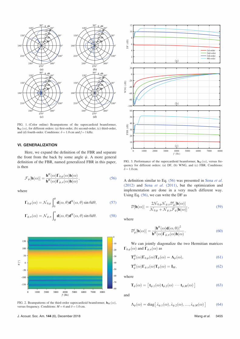
FIG. 1. (Color online) Beampatterns of the supercardioid beamformer,
hSCðxÞ, for different orders: (a) first-order, (b) second-order, (c) third-order,and (d) fourth-order. Conditions: d¼ 1.0 cm and f¼ 1 kHz.
FIG. 2. Beampatterns of the third-order supercardioid beamformer, hSCðxÞ,versus frequency. Conditions:M¼ 4 and d¼ 1.0 cm.
FIG. 3. Performance of the supercardioid beamformer, hSCðxÞ, versus fre-quency for different orders: (a) DF, (b) WNG, and (c) FBR. Conditions:
d¼ 1.0 cm.
J. Acoust. Soc. Am. 144 (6), December 2018 Wang et al. 3455

are the eigenvector and eigenvalue matrices of C�1w;pðxÞC0;wðxÞ,
respectively, and organized similarly to KðxÞ and TðxÞ. So, wehave
THw xð ÞC0;p xð ÞTw xð Þ ¼ 1
2N 0;wKw xð Þ þ 1
2N w;pIM:
(65)
Following the same steps as in Sec. VC, we can find a more
general reduced-rank filter,
hQ;w xð Þ ¼ P4;1:Q xð Þd x; 0ð ÞdH x; 0ð ÞP4;1:Q xð Þd x; 0ð Þ ; (66)
where
P4;1:QðxÞ ¼ Tw;1:QðxÞ� TH
w;1:QðxÞTw;1:QðxÞh i�1
THw;1:QðxÞ;
(67)
and Tw;1:QðxÞ is defined in a similar way to T1:QðxÞ. ForQ¼ 1, we get
h1;w xð Þ ¼ tw;1 xð ÞdH x; 0ð Þtw;1 xð Þ ; (68)
which is the beamformer obtained from maximization of
Fw½hðxÞ�.From the maximization of the DF in (59), we can derive
another reduced-rank filter,
hQ;2;w xð Þ ¼ P5;1:Q xð Þd x; 0ð ÞdH x; 0ð ÞP5;1:Q xð Þd x; 0ð Þ ; (69)
where
P5;1:Q xð Þ ¼ Tw;1:Q xð Þ
� 1
N 0;wKw;1:Q xð Þ þ 1
N w;pIQ
� ��1
THw;1:Q xð Þ;
(70)
and Kw;1:QðxÞ is defined analogously to K1:QðxÞ. It can be
verified that (see the Appendix)
F h1;2;wðxÞ� � � F h2;2;wðxÞ
� �� � � � � F hM;2;wðxÞ
� �; (71)
D h1;2;wðxÞ� � � D h2;2;wðxÞ
� �� � � � � D hM;2;wðxÞ
� �: (72)
We can also construct a regularized version of hQ;2;wðxÞ,i.e.,
FIG. 4. (Color online) Beampatterns of the beamformer hQ;RRðxÞ for differ-ent values of Q: (a) Q¼ 1, (b) Q¼ 2, (c) Q¼ 3, (d) Q¼ 4, (e) Q¼ 5, and (f)
Q¼ 6. Conditions: M¼ 6, d¼ 1.0 cm, and f¼ 1 kHz.
FIG. 5. Performance of the beamformer hQ;RRðxÞ versus frequency for dif-
ferent values of Q: (a) DF, (b) WNG, and (c) FBR. Conditions: M¼ 6 and
d¼ 1.0 cm.
3456 J. Acoust. Soc. Am. 144 (6), December 2018 Wang et al.

hQ;2;w;� xð Þ ¼ P6;1:Q xð Þd x; 0ð ÞdH x; 0ð ÞP6;1:Q xð Þd x; 0ð Þ ; (73)
where
P6;1:Q xð Þ ¼ Tw;1:Q xð Þ
� 1
N 0;wKw;1:Q xð Þ þ �
N w;pIQ
� ��1
THw;1:Q xð Þ:
(74)
The relations between D½hQ;2;w;�ðxÞ�; Fw½hQ;2;w;�ðxÞ�, and Q
and � are similar to those with the beamformer hQ;RR2;�ðxÞ.The particular case of Q¼M and �¼1 corresponds to
the beamformer obtained from maximization of D0w½hðxÞ� in
Eq. (60), i.e.,
hM;2;w;1 xð Þ ¼ C�1w;p xð Þd x; 0ð Þ
dH x; 0ð ÞC�1w;p xð Þd x; 0ð Þ : (75)
VII. SIMULATIONS
In this section, the performance of the proposed beam-
formers are evaluated in terms of beampattern, WNG, DF,
and FBR/GFBR.
A. Performance of the supercardioid beamformer
First, we investigate the performance of the supercardi-
oid beamformer. Figure 1 plots the beampatterns of this
FIG. 6. (Color online) Beampatterns of the beamformer hQ;RR2ðxÞ for dif-ferent values of Q: (a) Q¼ 1, (b) Q¼ 2, (c) Q¼ 3, (d) Q¼ 4, (e) Q¼ 5, and
(f) Q¼ 6. Conditions: M¼ 6, d¼ 1.0 cm, and f¼ 1 kHz.
FIG. 7. Performance of the beamformer hQ;RR2ðxÞ versus frequency for dif-
ferent values of Q: (a) DF, (b) WNG, and (c) FBR. Conditions: M¼ 6 and
d¼ 1.0 cm.
FIG. 8. (Color online) Beampatterns of the beamformer hQ;RR2;�ðxÞ for dif-ferent values of �: (a) �¼ 100, (b) �¼ 102, (c) �¼ 104, and (d) �¼ 106.
Conditions:M¼ 6, Q¼ 6, d¼ 1.0 cm, and f¼ 1 kHz.
J. Acoust. Soc. Am. 144 (6), December 2018 Wang et al. 3457

beamformer for different orders at f¼ 1 kHz. Figure 2 plots
the beampatterns of the third-order supercardioid beam-
former versus frequency. As can be seen, the obtained beam-
patterns are almost frequency invariant, except at very low
frequencies (f< 150Hz) due to numerical problems. The
DF, WNG, and FBR of the supercardioid beamformer versus
frequency for different orders are plotted in Fig. 3. One can
see from this figure that the DF and FBR increase with the
order, while the WNG decreases. Even though the supercar-
dioid beamformer can achieve maximum FBR, it suffers
from white noise amplification (very low WNG), and its DF
is also limited, which motivated us to develop the hQ;RRðxÞand hQ;RR2ðxÞ beamformers.
FIG. 9. Performance of the beamformer hQ;RR2;�ðxÞ versus frequency for
different values of �: (a) DF, (b) WNG, and (c) FBR. Conditions: M¼ 6,
Q¼ 6, and d¼ 1.0 cm.
FIG. 10. (Color online) Beampatterns of the beamformer hQ;wðxÞ with
different values of w: (a) w ¼ 30�, (b) w ¼ 60�, (c) w ¼ 90�, and (d)
w ¼ 120�. Conditions:M¼ 4, Q¼ 1, d¼ 1.0 cm, and f¼ 1 kHz.
FIG. 11. Beampatterns of the beamformer hQ;wðxÞ versus frequency.
Conditions:M¼ 4, w ¼ 60�, Q¼ 1, and d¼ 1.0 cm.
FIG. 12. Performance of the beamformer hQ;wðxÞ with different values of
w: (a) DF, (b) WNG, and (c) GFBR. Conditions: M¼ 4, Q¼ 1, and
d¼ 1.0 cm.
3458 J. Acoust. Soc. Am. 144 (6), December 2018 Wang et al.

B. Performance of the reduced-rank beamformers
In this subsection, the performance of the beamformer
hQ;RRðxÞ is investigated. We consider a ULA with M¼ 6
and d¼ 1.0 cm. Figure 4 plots the beampatterns of hQ;RRðxÞfor f¼ 1 kHz and different values of Q. As we can see, the
beampatterns of this beamformer vary significantly with Q.The beamwidth increases with the value of Q. When Q¼ 1,
we obtain the beampattern of the fifth-order supercardioid
beamformer, while when Q¼ 6, we get the beampattern of
the DS beamformer. The DF, WNG, and FBR of hQ;RRðxÞas a function of frequency for different values of Q are plot-
ted in Fig. 5. The beamformer hQ;RRðxÞ achieves the maxi-
mum FBR and high DF when Q¼ 1, but it suffers from
white noise amplification in this case, which is particularly
serious at low frequencies. When Q¼ 6, however, it obtains
the maximum WNG, but the FBR and DF are limited. From
Fig. 5, one can see that the WNG of the beamformer
hQ;RRðxÞ increases while the DF and FBR decrease with the
value of Q, which should be expected due to the form of
hQ;RRðxÞ in Eq. (34), except for some disturbances of the
DF and FBR at high frequencies. Clearly, the beamformer
hQ;RRðxÞ can achieve some tradeoff between the DF, FBR,
and WNG by adjusting the value of Q.
Next, we examine the performance of the beamformer
hQ;RR2ðxÞ. Again, a ULA with M¼ 6 and d¼ 1.0 cm is con-
sidered. The beampatterns of hQ;RR2ðxÞ are plotted in Fig. 6
for f¼ 1 kHz and different values of Q. As can be seen, the
beampatterns of this beamformer vary greatly with Q also.
The beamwidth decreases with the increase of Q. When
Q¼ 1 and 6, we get the beampatterns of the fifth-order
supercardioid beamformer and classical superdirective
beamformer (fifth-order hypercardioid), respectively. Figure
7 plots the DF, WNG, and FBR of hQ;RR2ðxÞ versus fre-
quency for different values of Q. The WNG and FBR of
hQ;RR2ðxÞ decrease with the increase of the value of Q, whilethe DF increases, which is consistent with the analysis,
except for some disturbances of the FBR at low frequencies
due to some numerical problems. Some of the curves are
very close to each other, since the performances of the beam-
former hQ;RR2ðxÞ when Q � 4 are similar for the given
microphone array, which can also be observed from the
beampatterns in Fig. 6. The beampatterns of hQ;RR2;�ðxÞ areplotted in Fig. 8 for Q¼ 6, f¼ 1 kHz, and different values of
�. Obviously, when �¼ 1, we have the beampattern of the
classical superdirective beamformer, and when �¼ 106, the
obtained beampattern is very close to that of the fifth-order
supercardioid beamformer. Figure 9 plots the DF, WNG, and
FBR of hQ;RR2;�ðxÞ versus frequency for Q¼ 6 and different
FIG. 13. (Color online) Beampatterns of the beamformer hQ;wðxÞ for differ-ent values of Q: (a) Q¼ 1, (b) Q¼ 2, (c) Q¼ 3, (d) Q¼ 4, (e) Q¼ 5, and (f)
Q¼ 6. Conditions: M¼ 6, w ¼ 60�, d¼ 1.0 cm, and f¼ 1 kHz.
FIG. 14. (Color online) Beampatterns of the beamformer hQ;2;wðxÞ for dif-ferent values of Q: (a) Q¼ 1, (b) Q¼ 2, (c) Q¼ 3, (d) Q¼ 4, (e) Q¼ 5, and
(f) Q¼ 6. Conditions: M¼ 6, w ¼ 120�, d¼ 1.0 cm, and f¼ 1 kHz.
J. Acoust. Soc. Am. 144 (6), December 2018 Wang et al. 3459
values of �. As can be seen, the WNG and FBR increase
with �, while the DF decreases, which is consistent with the
analysis, except for the FBR at low frequency bands.
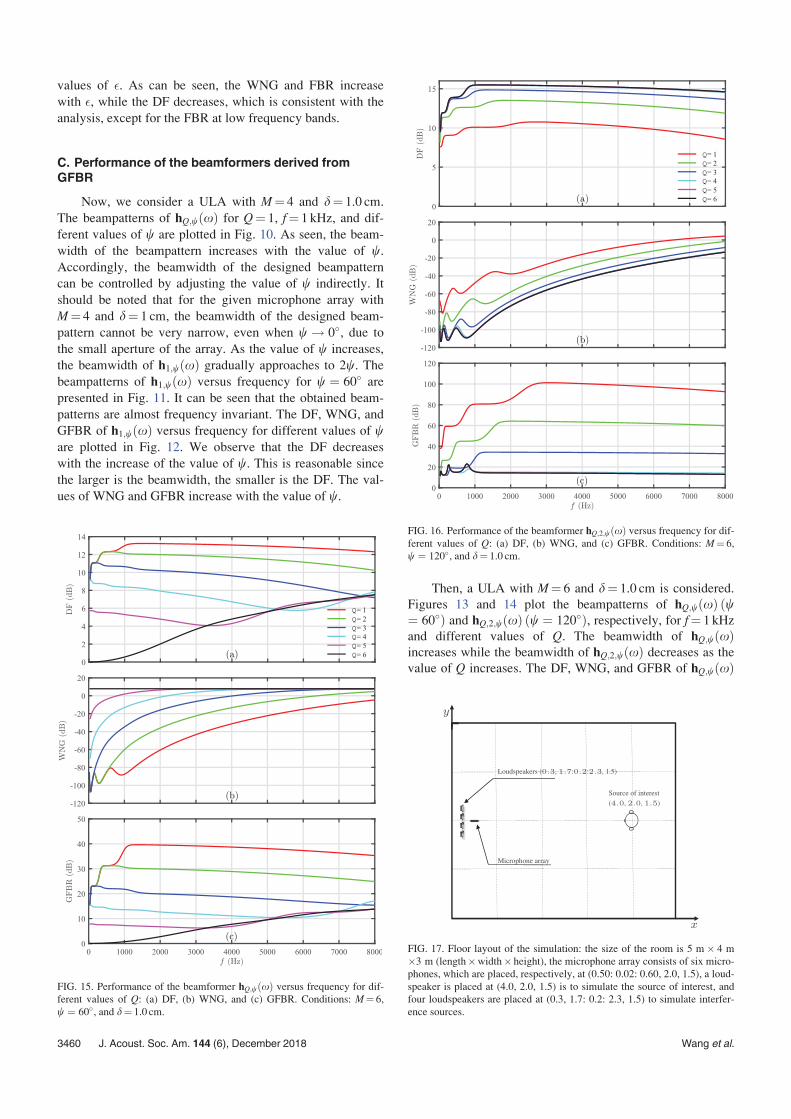
C. Performance of the beamformers derived fromGFBR
Now, we consider a ULA with M¼ 4 and d¼ 1.0 cm.
The beampatterns of hQ;wðxÞ for Q¼ 1, f¼ 1 kHz, and dif-
ferent values of w are plotted in Fig. 10. As seen, the beam-
width of the beampattern increases with the value of w.Accordingly, the beamwidth of the designed beampattern
can be controlled by adjusting the value of w indirectly. It
should be noted that for the given microphone array with
M¼ 4 and d¼ 1 cm, the beamwidth of the designed beam-
pattern cannot be very narrow, even when w ! 0�, due to
the small aperture of the array. As the value of w increases,
the beamwidth of h1;wðxÞ gradually approaches to 2w. Thebeampatterns of h1;wðxÞ versus frequency for w ¼ 60� are
presented in Fig. 11. It can be seen that the obtained beam-
patterns are almost frequency invariant. The DF, WNG, and
GFBR of h1;wðxÞ versus frequency for different values of ware plotted in Fig. 12. We observe that the DF decreases
with the increase of the value of w. This is reasonable since
the larger is the beamwidth, the smaller is the DF. The val-
ues of WNG and GFBR increase with the value of w.
Then, a ULA with M¼ 6 and d¼ 1.0 cm is considered.
Figures 13 and 14 plot the beampatterns of hQ;wðxÞ ðw¼ 60�Þ and hQ;2;wðxÞ ðw ¼ 120�Þ, respectively, for f¼ 1 kHz
and different values of Q. The beamwidth of hQ;wðxÞincreases while the beamwidth of hQ;2;wðxÞ decreases as thevalue of Q increases. The DF, WNG, and GFBR of hQ;wðxÞ
FIG. 15. Performance of the beamformer hQ;wðxÞ versus frequency for dif-
ferent values of Q: (a) DF, (b) WNG, and (c) GFBR. Conditions: M¼ 6,
w ¼ 60�, and d¼ 1.0 cm.
FIG. 16. Performance of the beamformer hQ;2;wðxÞ versus frequency for dif-
ferent values of Q: (a) DF, (b) WNG, and (c) GFBR. Conditions: M¼ 6,
w ¼ 120�, and d¼ 1.0 cm.
FIG. 17. Floor layout of the simulation: the size of the room is 5 m� 4 m
�3 m (length�width� height), the microphone array consists of six micro-
phones, which are placed, respectively, at (0.50: 0.02: 0.60, 2.0, 1.5), a loud-
speaker is placed at (4.0, 2.0, 1.5) is to simulate the source of interest, and
four loudspeakers are placed at (0.3, 1.7: 0.2: 2.3, 1.5) to simulate interfer-
ence sources.
3460 J. Acoust. Soc. Am. 144 (6), December 2018 Wang et al.
and hQ;2;wðxÞ as a function of frequency for different values
of Q are plotted in Figs. 15 and 16, respectively. The trends
of the DF, WNG, and GFBR versus the parameter Q agree
well with the analysis, except for some disturbances at low
frequencies due to numerical problems. It is clearly seen that
these developed beamformers facilitate tradeoffs among the
DF, WNG, and GFBR by adjusting the value of Q.
D. Performance in simulated reverberant roomenvironments
Finally, the performance of the developed beamformers
are evaluated in room acoustic environments simulated with
the widely used image model (Allen and Berkley, 1979;
Lehmanna and Johansson, 2008). The size of the simulated
room is 5m� 4m� 3m (length�width� height). For con-
venience of exposition, we denote the position in the room
as (x, y, z) with reference to a corner in a Cartesian coordi-
nate system. A microphone array consisting of six omnidi-
rectional microphones is used and the positions of the six
microphones are at (0.50: 0.02: 0.60, 2.0, 1.5) as illustrated
in Fig. 17. A loudspeaker, playing back a pre-recorded
speech signal, is placed at (4.0, 2.0, 1.5) to simulate a source
of interest. Four loudspeakers (e.g., from the sound bar of a
television) placed at (0.3, 1.7: 0.2: 2.3, 1.5) are used to
simulate interference sources. The room impulse responses
(RIRs) from every loudspeaker to the six microphones are
generated with the image model method (Allen and Berkley,
1979; Lehmanna and Johansson, 2008). The reflection coef-
ficients of all the six walls at set to 0.35 and the correspond-
ing reverberation time T60, i.e., the time for the sound to die
away to a level 60 decibels below its original level, which is
measured by the Schroeder’s method (Schroeder, 1965), is
approximately 100ms. The output signals of the micro-
phones are generated by convolving the source signal (pre-
recorded with a sampling rate of 16 kHz from a female
speaker in a quiet environment) with the RIRs from the posi-
tion of the source of interest to the array of microphones,
and then adding either spatially and temporally white
Gaussian noise or interference signals (generated by con-
volving another pre-recorded clean speech signal or white
Gaussian noise with the RIRs from the positions of the four
interference loudspeakers to the array of microphones).
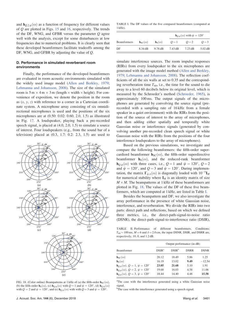
Based on the previous simulations, we investigate and
compare the following beamformers: the fifth-order super-
cardiord beamformer hSCðxÞ, the fifth-order superdirective
beamformer hSðxÞ, and the reduced-rank beamformer
hQ;wðxÞ with three cases, i.e., Q¼ 1 and w ¼ 120�, Q¼ 2
and w ¼ 120�, and Q¼ 3 and w ¼ 120�. During implemen-
tation, the matrix Cw;pðxÞ is diagonally loaded with 10�5IMfor numerical stability where IM is an identity matrix of size
M�M. The beampatterns at 1 kHz of these beamformers are
plotted in Fig. 18. The values of the DF of these five beam-
formers, which are computed at 1 kHz, are listed in Table I.
Besides the beampattern and DF, we also investigate the
array performance in the presence of white Gaussian noise,
interference, and reverberation. We divide the RIRs into two
parts: direct path and reflections, based on which we defined
three metrics, i.e., the direct-path-signal-to-noise ratio
(DSNR), the direct-path-signal-to-interference ratio (DSIR),
FIG. 18. (Color online) Beampatterns at 1 kHz of (a) the fifth-order hSCðxÞ,(b) the fifth-order hSðxÞ, (c) hQ;wðxÞ with Q¼ 1 and w ¼ 120�, (d) hQ;wðxÞwith Q ¼ 2 and w ¼ 120�, and (e) hQ;wðxÞ with with Q¼ 3 and w ¼ 120�.
TABLE I. The DF values of the five compared beamformers (computed at
1 kHz).
hQ;wðxÞ with w ¼ 120�
Beamformers hSCðxÞ hSðxÞ Q¼ 1 Q¼ 2 Q¼ 3
DF 8.34 dB 9.78 dB 7.43 dB 7.23 dB 5.02 dB
TABLE II. Performance of different beamformers. Conditions:
T60 100ms, M¼ 6 and d¼ 2.0 cm, the input DSNR, DSIR, and DSRR are,
respectively, 10, 0, and 1.2 dB.
Output performance (in dB)
Beamformer DSIRa DSIRb DSRR DSNR
hSCðxÞ 20.12 18.49 5.86 1.25
hSðxÞ 16.19 13.02 9.49 �12.54
hQ;wðxÞ; Q ¼ 1; w ¼ 120� 23.05 21.68 5.10 1.91
hQ;wðxÞ; Q ¼ 2; w ¼ 120� 19.68 16.03 4.58 11.06
hQ;wðxÞ; Q ¼ 3; w ¼ 120� 18.44 14.40 4.48 15.58
aThe case with the interference generated using a white Gaussian noise
signal.bThe case with the interference generated using a speech signal.
J. Acoust. Soc. Am. 144 (6), December 2018 Wang et al. 3461

direct-path-signal-to-reverberation ratio (DSRR). The input
DSNR and DSIR in this simulation are set to 10 and 0 dB,
respectively. The input DSRR for our simulation setup is
approximately 1.2 dB. To compute the output DSNR, DSIR,
and DSRR, we first divide the array output signals into frames
with a frame size of 256 samples (16-ms long) and an overlap
factor of 75%. The Kaiser window is applied to each frame to
deal with the frequency aliasing problem. Then, a 256-point fast
Fourier transform (FFT) is applied to the windowed signal frame
to transform the array signal into the short-time Fourier trans-
form (STFT) domain. In every STFT subband, a beamformer
filter is designed and applied to the array signals. The inverse
STFT (ISTFT) and overlap-add method are used to convert the
processed signals back to the time domain. We finally compute
the output DSNR, DSIR, and DSRR. We consider two cases. In
the first one, the interference signals are generated by convolv-
ing a white Gaussian noise signal with the RIRs from the four
interference loudspeakers to the microphones. In the second
case, the interference signals are generated by convolving a
speech signal (different from the source one) with the RIRs
from the four interference loudspeakers to the microphones. The
results of this case are summarized in Table II.
It is clearly seen from Table II the advantage of the
reduced rank beamformers.
VIII. CONCLUSIONS
Exploiting the performance measures FBR and GFBR,
we derived several kinds of beamformers, i.e., hSCðxÞ;hQ;RRðxÞ; hQ;RR2ðxÞ; hQ;RR2;�ðxÞ; hQ;wðxÞ; hQ;2;wðxÞ, andhQ;2;w;�ðxÞ. The beamformers hSCðxÞ and h1;wðxÞ maximize
the FBR and GFBR, respectively, and have almost frequency-
invariant beampatterns. The beamwidth of the beamformer
h1;wðxÞ can be changed by adjusting the value of w. The otherbeamformers enable us to compromise between the FBR/
GFBR and WNG or DF by adjusting the values of the param-
eters Q and/or �. The DS and classical superdirective beam-
formers are particular cases of the proposed framework.
ACKNOWLEDGMENTS
This work was supported by the Israel Science
Foundation (Grant No. 576/16), and the ISF-NSFC joint
research program (Grant Nos. 2514/17 and 61761146001),
and the NSFC Distinguished Young Scientists Fund (Grant
No. 61425005). The work of X.W. was supported in part by
the China Scholarship Council.
APPENDIX
D hQ;2;w;�ð Þ ¼dH 0ð ÞTw;1:Q
1
N 0;wKw;1:Q þ �
N w;pIQ
� ��1
THw;1:Qd 0ð Þ
" #2
dH 0ð ÞTw;1:Q1
N 0;wKw;1:Q þ �
N w;pIQ
� ��1
THw;1:QC0;pTw;1:Q
1
N 0;wKw;1:Q þ �
N w;pIQ
� ��1
THw;1:Qd 0ð Þ
¼ dH 0ð ÞTw;1:Q1
N 0;wKw;1:Q þ �
N w;pIQ
� ��1
THw;1:Qd 0ð Þ; (A1)
Fw hQ;2;w;�ð Þ ¼dH 0ð ÞTw;1:Q
1
N 0;wKw;1:Q þ �
N w;pIQ
� ��1
THw;1:QC0;wTw;1:Q
1
N 0;wKw;1:Q þ �
N w;pIQ
� ��1
THw;1:Qd 0ð Þ
dH 0ð ÞTw;1:Q1
N 0;wKw;1:Q þ �
N w;pIQ
� ��1
THw;1:QCw;pTw;1:Q
1
N 0;wKw;1:Q þ �
N w;pIQ
� ��1
THw;1:Qd 0ð Þ
¼dH 0ð ÞTw;1:Q
1
N 0;wKw;1:Q þ �
N w;pIQ
� ��1
Kw;1:Q1
N 0;wKw;1:Q þ �
N w;pIQ
� ��1
THw;1:Qd 0ð Þ
dH 0ð ÞTw;1:Q1
N 0;wKw;1:Q þ �
N w;pIQ
� ��1
IQ1
N 0;wKw;1:Q þ �
N w;pIQ
� ��1
THw;1:Qd 0ð Þ
: (A2)
Substituting Eq. (73) into Eq. (10), we obtain Eq. (A1) (where the parameter x is removed for concision), which can be
rewritten as
D hQ;2;w;� xð Þ� � ¼ XQi¼1
kw;i xð ÞN 0;w
þ �
N w;p
" #�1
jdH x; 0ð Þtw;i xð Þj2: (A3)
It is obvious that D½hQ;2;w;�ðxÞ� is an increasing function of Q, and a decreasing function of �. Substituting Eq. (73) into Eq.
(56), we obtain Eq. (A2) (where the parameter x is removed also for concision), which can be simplified as
3462 J. Acoust. Soc. Am. 144 (6), December 2018 Wang et al.
Fw hQ;2;w;� xð Þ� � ¼
XQi¼1
kw;i xð Þkw;i xð ÞN 0;w
þ �
N w;p
" #2jdH x; 0ð Þtw;i xð Þj2
XQi¼1
1
kw;i xð ÞN 0;w
þ �
N w;p
" #2jdH x; 0ð Þtw;i xð Þj2
: (A4)
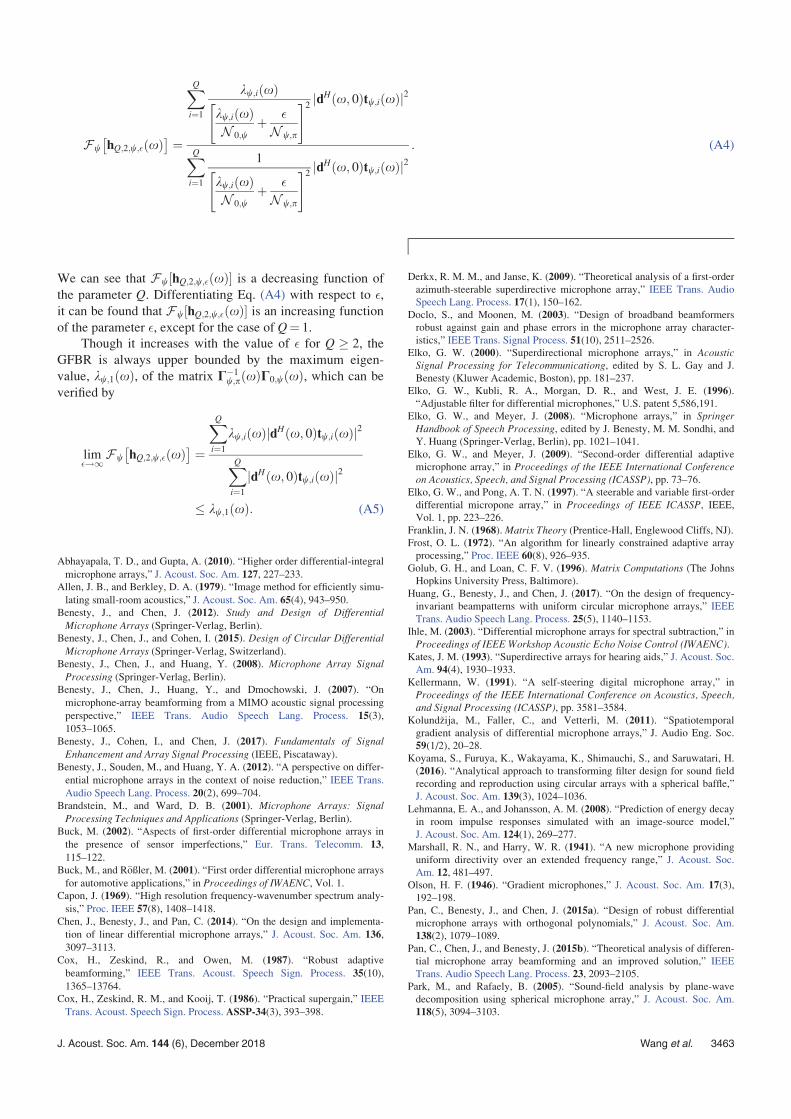
We can see that Fw½hQ;2;w;�ðxÞ� is a decreasing function of
the parameter Q. Differentiating Eq. (A4) with respect to �,it can be found that Fw½hQ;2;w;�ðxÞ� is an increasing function
of the parameter �, except for the case of Q¼ 1.
Though it increases with the value of � for Q � 2, the
GFBR is always upper bounded by the maximum eigen-
value, kw;1ðxÞ, of the matrix C�1w;pðxÞC0;wðxÞ, which can be
verified by
lim�!1Fw hQ;2;w;� xð Þ� � ¼
XQi¼1
kw;i xð ÞjdH x; 0ð Þtw;i xð Þj2
XQi¼1
jdH x; 0ð Þtw;i xð Þj2
� kw;1 xð Þ: (A5)
Abhayapala, T. D., and Gupta, A. (2010). “Higher order differential-integral
microphone arrays,” J. Acoust. Soc. Am. 127, 227–233.
Allen, J. B., and Berkley, D. A. (1979). “Image method for efficiently simu-
lating small-room acoustics,” J. Acoust. Soc. Am. 65(4), 943–950.
Benesty, J., and Chen, J. (2012). Study and Design of DifferentialMicrophone Arrays (Springer-Verlag, Berlin).
Benesty, J., Chen, J., and Cohen, I. (2015). Design of Circular DifferentialMicrophone Arrays (Springer-Verlag, Switzerland).
Benesty, J., Chen, J., and Huang, Y. (2008). Microphone Array SignalProcessing (Springer-Verlag, Berlin).
Benesty, J., Chen, J., Huang, Y., and Dmochowski, J. (2007). “On
microphone-array beamforming from a MIMO acoustic signal processing
perspective,” IEEE Trans. Audio Speech Lang. Process. 15(3),
1053–1065.
Benesty, J., Cohen, I., and Chen, J. (2017). Fundamentals of SignalEnhancement and Array Signal Processing (IEEE, Piscataway).
Benesty, J., Souden, M., and Huang, Y. A. (2012). “A perspective on differ-
ential microphone arrays in the context of noise reduction,” IEEE Trans.
Audio Speech Lang. Process. 20(2), 699–704.
Brandstein, M., and Ward, D. B. (2001). Microphone Arrays: SignalProcessing Techniques and Applications (Springer-Verlag, Berlin).
Buck, M. (2002). “Aspects of first-order differential microphone arrays in
the presence of sensor imperfections,” Eur. Trans. Telecomm. 13,
115–122.
Buck, M., and R€oßler, M. (2001). “First order differential microphone arrays
for automotive applications,” in Proceedings of IWAENC, Vol. 1.Capon, J. (1969). “High resolution frequency-wavenumber spectrum analy-
sis,” Proc. IEEE 57(8), 1408–1418.
Chen, J., Benesty, J., and Pan, C. (2014). “On the design and implementa-
tion of linear differential microphone arrays,” J. Acoust. Soc. Am. 136,
3097–3113.
Cox, H., Zeskind, R., and Owen, M. (1987). “Robust adaptive
beamforming,” IEEE Trans. Acoust. Speech Sign. Process. 35(10),
1365–13764.
Cox, H., Zeskind, R. M., and Kooij, T. (1986). “Practical supergain,” IEEE
Trans. Acoust. Speech Sign. Process. ASSP-34(3), 393–398.
Derkx, R. M. M., and Janse, K. (2009). “Theoretical analysis of a first-order
azimuth-steerable superdirective microphone array,” IEEE Trans. Audio
Speech Lang. Process. 17(1), 150–162.
Doclo, S., and Moonen, M. (2003). “Design of broadband beamformers
robust against gain and phase errors in the microphone array character-
istics,” IEEE Trans. Signal Process. 51(10), 2511–2526.
Elko, G. W. (2000). “Superdirectional microphone arrays,” in AcousticSignal Processing for Telecommunicationg, edited by S. L. Gay and J.
Benesty (Kluwer Academic, Boston), pp. 181–237.
Elko, G. W., Kubli, R. A., Morgan, D. R., and West, J. E. (1996).
“Adjustable filter for differential microphones,” U.S. patent 5,586,191.
Elko, G. W., and Meyer, J. (2008). “Microphone arrays,” in SpringerHandbook of Speech Processing, edited by J. Benesty, M. M. Sondhi, and
Y. Huang (Springer-Verlag, Berlin), pp. 1021–1041.
Elko, G. W., and Meyer, J. (2009). “Second-order differential adaptive
microphone array,” in Proceedings of the IEEE International Conferenceon Acoustics, Speech, and Signal Processing (ICASSP), pp. 73–76.
Elko, G. W., and Pong, A. T. N. (1997). “A steerable and variable first-order
differential micropone array,” in Proceedings of IEEE ICASSP, IEEE,Vol. 1, pp. 223–226.
Franklin, J. N. (1968).Matrix Theory (Prentice-Hall, Englewood Cliffs, NJ).
Frost, O. L. (1972). “An algorithm for linearly constrained adaptive array
processing,” Proc. IEEE 60(8), 926–935.
Golub, G. H., and Loan, C. F. V. (1996). Matrix Computations (The Johns
Hopkins University Press, Baltimore).
Huang, G., Benesty, J., and Chen, J. (2017). “On the design of frequency-
invariant beampatterns with uniform circular microphone arrays,” IEEE
Trans. Audio Speech Lang. Process. 25(5), 1140–1153.
Ihle, M. (2003). “Differential microphone arrays for spectral subtraction,” in
Proceedings of IEEE Workshop Acoustic Echo Noise Control (IWAENC).Kates, J. M. (1993). “Superdirective arrays for hearing aids,” J. Acoust. Soc.
Am. 94(4), 1930–1933.
Kellermann, W. (1991). “A self-steering digital microphone array,” in
Proceedings of the IEEE International Conference on Acoustics, Speech,and Signal Processing (ICASSP), pp. 3581–3584.
Kolund�zija, M., Faller, C., and Vetterli, M. (2011). “Spatiotemporal
gradient analysis of differential microphone arrays,” J. Audio Eng. Soc.
59(1/2), 20–28.
Koyama, S., Furuya, K., Wakayama, K., Shimauchi, S., and Saruwatari, H.
(2016). “Analytical approach to transforming filter design for sound field
recording and reproduction using circular arrays with a spherical baffle,”
J. Acoust. Soc. Am. 139(3), 1024–1036.
Lehmanna, E. A., and Johansson, A. M. (2008). “Prediction of energy decay
in room impulse responses simulated with an image-source model,”
J. Acoust. Soc. Am. 124(1), 269–277.
Marshall, R. N., and Harry, W. R. (1941). “A new microphone providing
uniform directivity over an extended frequency range,” J. Acoust. Soc.
Am. 12, 481–497.
Olson, H. F. (1946). “Gradient microphones,” J. Acoust. Soc. Am. 17(3),
192–198.
Pan, C., Benesty, J., and Chen, J. (2015a). “Design of robust differential
microphone arrays with orthogonal polynomials,” J. Acoust. Soc. Am.
138(2), 1079–1089.
Pan, C., Chen, J., and Benesty, J. (2015b). “Theoretical analysis of differen-
tial microphone array beamforming and an improved solution,” IEEE
Trans. Audio Speech Lang. Process. 23, 2093–2105.
Park, M., and Rafaely, B. (2005). “Sound-field analysis by plane-wave
decomposition using spherical microphone array,” J. Acoust. Soc. Am.
118(5), 3094–3103.
J. Acoust. Soc. Am. 144 (6), December 2018 Wang et al. 3463
Schelkunoff, S. A. (1943). “A mathematical theory of linear arrays,” Bell
Syst. Tech. J. 22(1), 80–107.
Schroeder, M. R. (1965). “New method for measuring reverberation time,”
J. Acoust. Soc. Am. 37, 409–412.
Sena, E. D., Hacihabiboglu, H., and Cvetkovic, Z. (2011). “A generalized
design method for directivity patterns of spherical microphone arrays,” in
Proceedings of the IEEE International Conference on Acoustics, Speech,and Signal Processing (ICASSP), pp. 125–128.
Sena, E. D., Hacihabiboglu, H., and Cvetkovic, Z. (2012). “On the design
and implementation of higher-order differential microphones,” IEEE
Trans. Audio Speech Lang. Process. 20(1), 162–174.
Sessler, G. M., and West, J. E. (1971). “Directional transducers,” IEEE
Trans. Audio Electroacoustic 19, 19–23.
Slavin, M. J. (1987). “Differential hearing aid with programmable frequency
response,” J. Acoust. Soc. Am. 81(5), 1657.
Song, H., and Liu, J. (2008). “First-order differential microphone array for
robust speech enhancement,” in Audio, Language and Image Processing,2008. ICALIP 2008. International Conference, pp. 1461–1466.
Teutsch, H., and Elko, G. W. (2001). “First- and second-order adap-
tive differential microphone arrays,” in Proceedings of IWAENC,IEEE.
Torres, A. M., Cobos, M., Pueo, B., and Lopez, J. J. (2012). “Robust acoustic
source localization based on modal beamforming and time–frequency process-
ing using circular microphone arrays,” J. Acoust. Soc. Am. 132(3), 1511–1520.
Uzkov, A. I. (1946). “An approach to the problem of optimum directive
antenna design,” in Comptes Rendus (Doklady) de l’Academie desSciences de l’URSS, pp. 35–38.
Wang, Y., Yang, Y., Ma, Y., and He, Z. (2014). “Robust high-order superdir-
ectivity of circular sensor arrays,” J. Acoust. Soc. Am. 136(4), 1712–1724.
Warren, D. M., and Thompson, S. (2006). “Microphone array having a sec-
ond order directional pattern,” U.S. patent 7,065,220.
Weinberger, J., Olson, H. F., and Massa, F. (1933). “A uni-directional rib-
bon microphone,” J. Acoust. Soc. Am. 5(2), 139–147.
Yan, S., Sun, H., Svensson, U. P., Ma, X., and Hovem, J. M. (2011).
“Optimal modal beamforming for spherical microphone arrays,” IEEE
Trans. Audio Speech Lang. Process. 19(2), 361–371.
Zhao, L., Benesty, J., and Chen, J. (2014). “Design of robust differential
microphone arrays,” IEEE Trans. Audio Speech Lang. Process. 22(10),
1455–1466.
Zheng, Y. R., Goubran, R. A., and El-Tanany, M. (2004). “Experimental
evaluation of a nested microphone array with adaptive noise cancellers,”
EEE Trans. Instrum. Meas. 53(3), 777–786.
3464 J. Acoust. Soc. Am. 144 (6), December 2018 Wang et al.