Microlocal analysis of synthetic aperture radar imaging in

Journal of Physics Conference Series

OPEN ACCESS

Microlocal analysis of synthetic aperture radarimaging in the presence of a vertical wallTo cite this article R Gaburro and C Nolan 2008 J Phys Conf Ser 124 012025

View the article online for updates and enhancements

You may also likeCancellation of singularities in SAR forcurved flight paths and non-flat topographyAndrew Homan

-

An efficient reconstruction approach for aclass of dynamic imaging operatorsB N Hahn and M-L Kienle Garrido

-

Microlocal analysis for spherical Radontransform two nonstandard problemsLinh V Nguyen and Tuan A Pham

-

This content was downloaded from IP address 12155205184 on 16022022 at 1355

Microlocal analysis of synthetic aperture radar

imaging in the presence of a vertical wall

Romina Gaburro and Clifford Nolan

Department of Mathematics and Statistics University of Limerick Castletroy Ireland

E-mail rominagaburroulie cliffordnolanulie

Abstract We consider the problem of imaging a target located nearby a perfectly reflectivevertical wall by making use of a SAR system in the case where a single pass is made overthe scene of which we expect to be able to reconstruct a two-dimensional image Many of theconventional methods make the assumption that the wave has scattered just once from theregion to be imaged before returning to the sensor to be recorded The purpose of this paperis to give a brief idea about how this restriction can be partially removed from a microlocalanalysis point of view in the case where the radar is operating with a poor directivity Thesimple case where the antenna is flying perpendicularly to the wall is presented here while amore in-depth study of this method will be analyzed elsewhere

1 Introduction

In Synthetic Aperture Radar (SAR) imaging a plane or a satellite carrying an antenna movesalong a flight track The antenna emits pulses of electromagnetic radiation which scatter offthe terrain and the scattered waves are detected with the same antenna The received signalsare then used to produce an image of the terrain (see [1] [5] [6] [7])

The nature of the imaging problem depends on the directivity of the antenna Here we areinterested in the case where the antenna has poor directivity and a typical example of that isthe foliage-penetrating radar (see [6] [10] [11]) whose low frequencies do not allow for muchbeam focusing

We consider the case when the target to be imaged is located nearby a perfectly reflectivevertical wall and a single pass along a straight line perpendicular to the wall is made over thescene The purpose of this paper is to give the reader an understanding of the method used inthe case of the most simple setting where the antenna is flying perpendicularly to the verticalwall In this situation in fact the calculations involved simplify quite a lot and allow perhapsthe reader to become more familiar with the tools of microlocal analysis For a more in-depthanalysis of this problem the authors refer to [3]

The data collected depend on two variables namely the (fast) time variable and the positionof the antenna along the flight track (slow variable) Because the data depend on two degreesof freedom we expect to be able to reconstruct a two-dimensional image of the scene

The high-frequency deviation of the speed of wave propagation from that in air is knownas the ground reflectivity function The forward scattering operator (by definition) maps thereflectivity function to the scattered waves that are recorded by the same emitting antenna(ie the antenna acts as a source and receiver) and it turns out to be a sum of four forward

4th AIP International Conference and the 1st Congress of the IPIA IOP PublishingJournal of Physics Conference Series 124 (2008) 012025 doi1010881742-65961241012025

ccopy 2008 IOP Publishing Ltd 1

operators if the target is located in the vicinity of a perfectly reflective vertical wall (see [3] [8])These correspond to the different paths that the wave can take when scattering to and fromthe ground For example the wave may scatter directly to and from the ground or it may firstscatter from the wall and then off the ground etc To obtain an image we must backprojectthe data which means applying a sum of four adjoint scattering operators to the data Thisleads to sixteen possible contributions to the image There is a lot of symmetry and we areable to analyze the resulting image We show that in the case of poor directivity it is possiblehave artifacts in the image We indicate the relationship between position of the true scattererand the artifact in the simple setting when the antenna is flying at a fixed height and along astraight line perpendicular to the vertical wall In the case that one can beam form adequatelyand direct the beam to a sufficiently small locality on the ground we show that these artifactscan be avoided

A weak-scattering approximation is used to model the scattered field which makes the forwardscattering operator a linear one Moreover the operator in question is a Fourier Integral Operator(FIO) (see [2] [4] [8] [9])and so are the four operators which are contributing to it Suchoperators map singular distributions to other singular distributions and the relationship betweenthe input and the output singularities forms what is called a canonical relation Canonicalrelations associated to FIOs are Lagrangian manifolds and have a rich geometric structure(see [3] [2] [7]) The authors study this in detail for the case when the antenna is flyingperpendicularly to a perfectly reflective vertical wall The outline of the paper is as follows Insection 2 we present a scattering model for the scattering operator in the presence of a verticalwall This is achieved through the use of method of images ([3]) In section 3 we show thecanonical relation is composed of four separate canonical relations Each one is associated tothe different ways in which the wave can scatter between the scene and wall To obtain an imagewe compose the adjoint scattering operator with the scattering operator itself The singularitiesin the resulting image are analyzed by examining the composition of the canonical relation forthe adjoint operator with the canonical relation of the scattering operator This analysis leadsto the results stated in the previous paragraph

2 The mathematical model of scattering

21 The forward operatorWe use the simple scalar wave equation to model the wave propagation

(

nabla2 minus1

c2(x)part2

t

)

U(t x) = f (1)

where f denotes the source and the function c is the wave propagation speed Although thecorrect model is Maxwellrsquos equations (1) is commonly used in SAR and represents a good modelfor sonar and ultrasound for example As in [3] [8] we make the following assumptions

Assumption 1 We assume that the target is well separated from the region where the sensorsare located and that in the intervening region c(x) = c0 where c0 is the (assumed constant) speedof light in air

Assumption 2 We assume that the target to be imaged is a-priori known to lie on the groundand lies strictly on one (known) side of a vertical wall We assume that the ground is locallyflat so if we denote by (x1 x2 x3) the cartesian coordinates in R3 then the ground can be locallyidentified with R2 = (x1 x2 0) | xi isin R i = 1 2 sube R3The vertical wall can be taken for simplicity as the infinite vertical plane x1 = 0 so we canidentify the area to be imaged by the set R2

+ = (x1 x2 0) | xi isin R i = 1 2 x1 gt 0


2

We denote by

Γ+ =

Γ+(s) | smin lt s lt smax

the straight line along which the antenna is moving along (flight track)There are four ways for the wave to hit the target on the ground and return to the antenna

Indeed the wave may scatter directly to and from the target Or the wave may scatter first fromthe wall then from the target and finally back to the antenna The third means of scatteringis the reverse of the former and finally the last method involves scattering from the wall on theway down to the target and again on the way back to the antenna The data that is collectedcontains all four kinds of scattering events in it See Figure 1 for an illustration of this

(s)

x

1

23

4

(s)ΓΓ+

minus

Figure 1 In case 1 the wave scatters directly to and from the target In case 2 the wavescatters from the wall to the target and back to the receiver In case 3 the wave scatters fromthe target to the wall and back to the receiver Finally in case 4 the wave scatters to the wallto the target and back to the wall again before returning to the receiver

We represent the (perfectly reflecting) wall via the method of images by placing a virtualsource at Γminus(s) symmetrically on the other side of the wall from the actual source location(Γ+(s)) (see [3] [8]) Note that the argument s in Γplusmn(s) denotes the current real (+ subscript)and virtual source position (minus subscript) respectively as it is moved over a path parametrizedby s

Let us recall that the scattering region is R2+ the data space parameters are (smin smax) times

[0 T ] and introduce the reflectivity function V (x) = 1c20

minus 1c2(x)

which encodes rapid changes in

material properties For example when the radio wave impinges on a building on the groundthe propagation speed changes suddenly according to the building materialsThen the scattering operator F from ldquoscenerdquo V (x) at the point x isin R2

+ to the collected datad(s t) at the time t isin [0 T ] and location s (ie at the antenna location Γ+(s)) is given by


3

d(s t) = FV (s t) =

int

eminusiω(

tminus2|zminusΓ+(s)|c0)

a1(x s t ω) V (z) dω dz

minus

int

eminusiω(

tminus(|zminusΓ+(s)|+|zminusΓminus(s)|)c0)


minus

int

eminusiω(



+

int

eminusiω(

tminus2|zminusΓminus(s)|c0)


= F1 V (s t) + F2 V (s t) + F3 V (s t) + F4 V (s t) (2)

The amplitudes ai i = 1 4 are geometrical optics amplitudes and encode the geometricalspreading beam pattern etc for the emitted and measured waves therefore they are knownquantities For more detail on this we refer to [3] We wish to reconstruct the unknown functionV from the data d ie solve an inverse problem

22 Statement of the inverse problemThe idealized inverse problem consists in determining V from the knowledge of d(s t) for any(s t) isin [smin smax] times [0 T ] for some T The amplitudes ai i = 1 4 appearing in (2) reflectthe four ways for the wave to scatter on its way from the source to the target and back to thereceiver location againFor technical reasons we need to assume

Assumption 3 For 1 le j le 4 the amplitude aj satisfies

sup(s t x)isinK

| part αω part β

s part δt part ρ

x aj(x s t ω) |le CjK α β δ ρ(1 + ω2)(2minus|α|)2 (3)

where K is any compact set in [smin smax]times [0 T ]timesR2+ and α β δ ρ are arbitrary multi-indices

of the appropriate dimension

The above assumption is valid for example when the waveform sent to the antenna isapproximately a delta function and the antenna is sufficiently broadband (see [3] [5]) Note

that the coefficients CjK α β δ ρ are constants depending only on their indices

Assumption 3 implies that the forward operators Fj 1 le j le 4 are Fourier Integral Operators(FIOs) (see [2] [3] [4] [8] [9])

3 Analysis of the scattering operator

31 Fourier Integral Operators (FIOs)We saw in section 2 that Fi 1 le i le 4 is a FIO and standard arguments in FIO theory give usinformation about how Fi 1 le i le 4 maps singularities from the scene into the data We willreview this below and to begin with we recall the following

DEFINITION 31 Let X = R2+ Y = (smin smax) times [0 T ] E prime(X ) E prime(Y) be the spaces of

distributions with compact support in X and Y respectively If F is a Fourier Integral Operator

F E prime(X ) minusrarr E prime(Y)

given by the oscillatory integral

Fu(y) =

int

eiφ(y x ω) a(y x ω) u(x) dω dx (4)


4

for any u isin E prime(X ) then its (twisted) canonical relation is the set

ΛprimeF =

(

(y η) (x ξ))

isin T (Y times X ) 0 | (y x ω) isin Cφ cap EssSupp(a)

η = Dyφ(y x ω) ξ = minusDxφ(y x ω)

(5)

where Dx and Dy denote the gradients with respect to the x and y variable respectively and 0is the zero section of T lowast(X times Y) The set Cφ is defined as the critical set points

Cφ =

(y x ω) | Dωφ(y x ω) = 0

(6)

which is called the critical manifold and EssSupp(a) is defined via its complement

CEssSupp(a) =(y x ω) | a(y x ω) and its derivatives decrease faster

than any negative power of ω as | ω |rarr infin

Note that the frequency ω can be multi-dimensional

DEFINITION 32 If we denote by Dprime(X ) the set of distributions on X and if u isin Dprime(X ) thenthe wave front set WF(u) of u is defined as the complement in T X 0 of the collection ofall (x ξ) isin T X 0 such that there exists a neighborhood U of x and a neighborhood U of ξsuch that for any ϕ isin Cinfin

0 (U) with x isin supp(ϕ) and any N isin N

F(ϕ u)(τξ) = O(τminusN ) for τ rarr infin uniformly in ξ isin U

Here F(ϕ u) denotes the Fourier transform of ϕ u

WF(u) is a closed cone in T X 0 and its singular support satisfies singsupp(u) =π(

WF (u))

where π is the natural projection of T X 0 into X (see [2])

DEFINITION 33 If F is given by (4) with distributional kernel KF isin Dprime(Y timesX ) given by theoscillatory integral

KF (y x) =

int

eiφ(y x ω)a(y x ω) dω

the wavefront relation WFprime(F) is defined by

WF prime(F ) =

(

(y η) (x ξ))

isin T (Y times X ) 0 | (y x η minusξ) isin WF (KF )

It turns out (see [2]) that

WF (Fu) sube WF prime(F ) WF (u)

WF prime(F ) sube ΛprimeF

(7)

whereldquordquo stands for the following composition

WF prime(F ) WF (u) = (y η)| exist ((y η) (x ξ)) isin WF prime(F ) (x ξ) isin WF (u) (8)

Let us compute the canonical relations ΛprimeFi

1 le i le 4 Note that ΛprimeF2

= ΛprimeF3

so we will onlycompute Λprime

Fi i = 1 2 4


5

32 The canonical relationsWe start by making the following assumption

Assumption 4 The antenna is flying perpendicular to the wall x1 = 0 at constant height hie

Γ+(s) = (γ1(s) 0 h) = (γ1 0 h)

Γminus(s) = (minus γ1(s) 0 h) = (minus γ1 0 h)

so that with arc length as the parametrisation the real and the virtual velocity fields are asfollows

Γ+(s) = V+ = (1 0 0)

Γminus(s) = Vminus = (minus1 0 0)

where Γ denotes the derivative of Γ with respect to s

With appropriate time units we may take c0 = 1 Define

R+ =[

(x1 minus γ1)2 + x2

2 + h2]12

=| x minus Γ+(s) | (9)

Rminus =[

(x1 + γ1)2 + x2

2 + h2]12

=| x minus Γminus(s) | (10)

so that the (twisted) canonical relations ΛprimeFi

1 le i le 4 associated to the operators Fi 1 le i le 4are respectively (see [3])

ΛprimeF1

=

(

(s t σ τ) (x ξ))

| t = 2 R+

σ = 2τx1 minus γ1

R+

τ = minusω

ξ = minus2τ (x minus Γ+(s))

(11)

ΛprimeF2

=

(

(s t σ τ) (x ξ))

| t = (R+ + Rminus)

σ = τ(x1 minus γ1

R+minus

x1 + γ1

Rminus

)

τ = minusω

ξ = minusτ(

(x minus Γ+(s)) + (x minus Γminus(s)))

(12)

ΛprimeF4

=

(

(s t σ τ) (x ξ))

| t = 2 Rminus

σ = minus2τx1 + γ1

Rminus

τ = minusω

ξ = minus2τ (x minus Γminus(s))

(13)


6

where for any non-zero vector v isin R3 we denote by |v| its length (ie its Euclidean norm) andwe define v = v

|v|

Forming an image usually involves operating on the data with a weighted adjoint operator(the reason for this will become clear soon) The forward map is given by the four contributions

F = F1 + F2 + F3 + F4

and the adjoint of F F by

F = F 1 + F

2 + F 3 + F

4

where F i is the adjoint of Fi Singularities in the scene will be mapped into singularities in

the data by any of the Fi while singularities in the data will be mapped into singularities in thescene by the adjoint maps F

i Our goal is to analyse the resulting image determine which kind of artifacts it may contain

and see if we can avoid them To do so we will see that we need to analyse the composition ofthe (twisted) canonical relations

ΛprimeF

i Λprime

Fj for any 1 le i j le 4 (14)

where

ΛprimeF

i= tΛprime

Fi for any 1 le i le 4

and the superscript t denotes the transposed relationThe reason for this is that if we denote by I the reconstructed image FIO theory implies

WF (I) sube WF prime(F ) WF prime(F ) WF (V )

sube

4⋃

ij=1

Λprimei Λprime

j

WF (V )(15)

Compositions in (14) and (15) are meant as compositions of relations ie if R1 sub U times V R2 sub V times W are relations then the composition R1 R2 sub U times W is defined by

R1 R2 =

(u w) isin U times W existv isin V (u v) isin R1 and (v w) isin R2

For any i j = 1 4 we will sometimes refer in the sequel to the case or pair (i j) orspeak about interaction between experiments i and j by meaning we are analysing the objectΛprime

F i Λprime

Fj(or similarly Λprime

F j Λprime

Fi) and we will call it backprojection (of the data)

33 Analysis of the diagonal termsWe need only analyze Λprime

F 2 Λprime

F2(pair (2 2)) among the diagonal compositions in (14) as pair

(1 1)(and similarly (4 4)) have been studied in [5] while case (3 3) is very similar to (2 2)Let us denote by x = (x1 x2 0) a point on the ground By defining the quantity

p =σ

τ (16)

and recalling (12) we have


7

x1 minus γ1

R+minus

x1 + γ1

Rminus= p (17)

R+ + Rminus = t (18)

Notice that the travel time condition given by (18) describes for any s and t the intersection ofan ellipsoid (whose foci are Γ+(s) Γminus(s)) with the earthrsquos surface In our specific case where theearth is locally flat this intersection is an ellipse The equation of this ellipse can be obtainedby squaring (18) a couple of times and rearranging to get

x22 =

( t2

4minus γ2

1 minus h2)

+(4γ2

1

t2minus 1

)

x21 (19)

One can directly verify the identity

4γ1x1 = R2minus minus R2

+ (20)

and by substituting Rminus = t minus R+ in the latter equation and rearranging it we obtain

x1 =t

4γ1

(

t minus 2R+

)

(21)

Substituting (21) into (17) we obtain the following quadratic equation for R+

R2+ minus tR+ +

α

4= 0 (22)

with

α =t(t2 minus 4γ2

1)

(t + pγ1) (23)

giving two possible solutions

R+ =t plusmn (t2 minus α)12

2

but R+ lt t2 which leaves the unique solution

R+ =t minus (t2 minus α)12

2 (24)

By (24) and (21) we finally get

x1 =t(t2 minus α)12

4γ1 (25)

so that x1 is uniquely determined If we operate the radar in side-scan mode ie we illuminateonly one side of the projected flight path on the ground x2 is uniquely determined (no signambiguity) by (19) and since x3 = 0 for a scatterer on the ground we have that the scattererlocation x is determined This shows that there are no artifacts present in the image obtainedfrom experiment 2 in the case when the radar is operated in side-scan mode

Remark 31 (See [3])0 lt α lt t2 (26)

The latter inequality guarantees a real root in (25)


8

331 Analysis of the non-diagonal terms We analyze the relations ΛprimeF lowast

i Λprime

F lowast

jfor i 6= j in

this subsection Again we assume that the antenna is flying perpendicularly to the wall ieAssumption 4 holds In that case we have

σ1 =2τ

c0

x1 minus γ1

R+(27)

σ2 = σ3 =τ

c0

(x1 minus γ1

R+minus

x1 + γ1

Rminus

)

(28)

σ4 = minus2τ

c0

x1 + γ1

Rminus (29)

Notice that

σ1 |x1=0= σ2 |x1=0= σ3 |x1=0= σ4 |x1=0= minus2τ

c0

γ1

R+ |x1=0lt 0

and

limx1rarrinfin

σ1(x) =2τ

c0 lim

x1rarrinfinσ2(x) = lim

x1rarrinfinσ3(x) = 0 lim

x1rarrinfinσ4(x) = minus

2τ

c0

Moreover

partx1R+ = Rminus1

+ (x1 minus γ1) (30)

partx1Rminus = Rminus1

minus (x1 + γ1) (31)

and

partx1σ1 =

2τ

c0

R+ minus (x1 minus γ1)partx1R+

R2+

=2τ

c0

R2+ minus (x1 minus γ1)

2

R3+

(32)

partx1σ2 = partx1

σ3 =τ

c0


R2+

minusR2

+ minus (x1 minus γ1)2

R3+

=τ

c0

(x22 + h2)(R3

minus minus R3+)

(R+Rminus)3(33)

partx1σ4 =

2τ

c0

Rminus minus (x1 minus γ1)partx1Rminus

R2minus

= minus2τ

c0

R2minus minus (x1 + γ1)

2

R3minus

(34)

By (9) (10) we have that R+ gt (x1 minus γ1) and Rminus gt (x1 + γ1) which imply that partx1σ1 gt 0

and partx1σ4 lt 0 respectively ie σ1 is increasing and σ4 is decreasing in the x1-direction

Moreover Rminus gt R+ gt 0 as the target is located on the right hand side of the vertical wallx1 = 0 which implies that partx1

σ2 gt 0 partx1σ3 gt 0 ie σ2 σ3 are increasing in the x1-

direction Therefore itrsquos impossible to get a common value between σ1 and σ4 and betweenσ2 or σ3 and σ4 We can therefore conclude that the composition in (14) is empty for the pairs


9

-1

-08

-06

-04

-02

0

02

04

06

08

1

0 100 200 300 400 500

sigm

a

x

h=50

sigma1sigma2sigma4

Figure 2 Figure shows thegraph of σ1 σ2 and σ4 when theantenna is flying on a straight lineperpendicular to the wall at thefixed height of h = 50 and thesource location is Γ+ = (50 250 50)

-1

-08

-06

-04

-02

0

02

04

06

08

1

0 100 200 300 400 500

sigm

a

x

h=100

sigma1sigma2sigma4

Figure 3 Figure shows thegraph of σ1 σ2 and σ4 when theantenna is flying on a straightline perpendicular to the wall atthe fixed height of h = 100and the source location is Γ+ =(50 250 100)

(i j) = (1 4) (4 1) (2 4) (4 2) (3 4) (4 3) (see Figures 2 and 3)

Let us consider pairs (i j) = (1 2) (2 1) Cases (i j) = (1 3) (3 1) can be treated in asimilar way We assume again that Assumption 4 holds and we denote by x = (x1 x2 0) andz = (z1 z2 0) two points on the ground In order to compose ΛF lowast

1ΛF2

(or similarly ΛF lowast

2ΛF1

)at points x z we must have (for coincidence of σ values)

2z1 minus γ1

Rz+

=

(

x1 minus γ1

Rx+

minusx1 + γ1

Rxminus

)

(35)

moreover x z must satisfy the two travel time conditions respectively

Rx+ + Rx

minus = t (36)

2Rz+ = t (37)

where we have used the notation Rx+ for R+ defined in (9) for the scattering point x and Rz

+

when the scattering point x is replaced by z etcBy combining (35) (36) and (37) we obtain

t(t minus Rx+)(x1 minus γ1) minus tRx

+(x1 + γ1) = 4RP+(t minus Rx

+)(z1 minus γ1) (38)

from which we extract the following expression for z1 as a function of x

z1 =[

(

4(Rx+)2 + t2 minus 4tRx

+

)

γ1 +(

2tRx+ minus t2

)

x1

]

4((Rx+)2 minus tRx

+) (39)

Using equations (22) and (24) it follows that

z1 =

(

t2 minus α

4γ1α

)

(

t2 minus 4γ21

)

(40)

which in turn implies that


10

z1 minus x1 =[

(t2 minus α)(t2 minus 4γ21)α minus t(t2 minus α)12

]

α (41)

The above formula gives us the relation between the first component x1 and z1 of two pointson the ground (scene) x = (x1 x2 0) and z = (z1 zeta 0) such that

(

(

x ξ)

(

z ζ)

)

isin ΛF lowast

1 ΛF2

(or similarly(

(

z ζ)

(

x ξ)

)

isin ΛF lowast

2 ΛF1

) Such points x z are therefore the images obtained

by backprojecting the same data therefore one of them (say x) must be the real scatterer andthe other one must be an artifact

Note that α (defined in (23)) is a function of p which is a function of x1 Therefore (41)gives us a formula for the distance between z1 and x1 in terms of x1 It follows that if we want toavoid artifacts resulting from backprojecting with (possibly weighted) operators F lowast

i i = 1 2 wemust ensure that the beam width in the first coordinate direction is smaller than that predictedby the right hand side of (41) Note that this implies a variable beam width restriction whichdepends on the (x1) location that is being illuminated for imaging This beam forming can bedone synthetically and it therefore does not impose extra logistical difficulties in acquiring thedata We can in fact superimpose the signals coming from each component of the antenna arrayto constructively and destructively interfere at particular locations on the ground This can bedone synthetically without the need to physically beam form at the time of the experimentIf the required beam forming is not possible then artifacts will be present and their locationcan be predicted by equation (41) in conjunction with (37) ie by intersecting a line with acircle on the ground Of course this may not be a complete determination if the usual left-rightambiguity of radar is still present (due to not being able to operate in side-scan mode)

Acknowledgments

RG and CN acknowledge the support of Science Foundation Ireland (Grant 03IN3I401)RG would also like to acknowledge the financial support of the Mathematics ApplicationsConsortium for Science and Industry (MACSI wwwmacsiie) funded under the ScienceFoundation Ireland Mathematics Initiative 06MI005

References[1] Cheney M 2001 A mathematical tutorial on synthetic aperture radar SIAM Review 43 pp 301-12[2] Duistermaat J J 1996 Fourier Integral Operators (Boston Birkhauser)[3] Gaburro R and Nolan C J 2007 Enhanced imaging from multiply scattered waves to appear in Inverse

Problems and Imaging[4] Grigis A and Sjostrand J 1994 Microlocal Analysis for Differential Operators An Introduction (London

Mathematical Society Lecture Note Series) vol 196 (Cambridge Cambridge University Press)[5] Nolan C J and Cheney M 2002 Synthetic aperture inversion Inverse Problems 18 pp 221-36[6] Nolan C J and Cheney M 2003 Synthetic aperture inversion for arbitrary flight paths and non-flat topography

IEEE Trans on Image Processing 12 pp 1035-43[7] Nolan C J and Cheney M 2004 Microlocal analysis of synthetic aperture radar imaging J Fourier Analysis

and its Applications 10 pp 133-48[8] Nolan C J Cheney M Dowling T and Gaburro R 2006 Enhanced angular resolution from multiply scattered

waves Inverse Problems 22 pp 1817-34[9] Treves F 1980 Introduction to Pseudodifferential and Fourier Integral Operators vol 1 and 2 (New York

Plenum Press)[10] Ulander L M H and Frolund P O 1998 Ultra-wideband SAR interferometry IEEE Trans GeosciRemote

Sensing 36 pp 1540-50[11] Ulander L M H and Hellsten H 1999 Low-frequency ultra-wideband array-antenna SAR for stationary and

moving target imaging Conf SPIE 13th Annuual Int Symp on Aerosense Orlando FL


11

Microlocal analysis of synthetic aperture radar

imaging in the presence of a vertical wall

Romina Gaburro and Clifford Nolan

Department of Mathematics and Statistics University of Limerick Castletroy Ireland

E-mail rominagaburroulie cliffordnolanulie

Abstract We consider the problem of imaging a target located nearby a perfectly reflectivevertical wall by making use of a SAR system in the case where a single pass is made overthe scene of which we expect to be able to reconstruct a two-dimensional image Many of theconventional methods make the assumption that the wave has scattered just once from theregion to be imaged before returning to the sensor to be recorded The purpose of this paperis to give a brief idea about how this restriction can be partially removed from a microlocalanalysis point of view in the case where the radar is operating with a poor directivity Thesimple case where the antenna is flying perpendicularly to the wall is presented here while amore in-depth study of this method will be analyzed elsewhere

1 Introduction

In Synthetic Aperture Radar (SAR) imaging a plane or a satellite carrying an antenna movesalong a flight track The antenna emits pulses of electromagnetic radiation which scatter offthe terrain and the scattered waves are detected with the same antenna The received signalsare then used to produce an image of the terrain (see [1] [5] [6] [7])

The nature of the imaging problem depends on the directivity of the antenna Here we areinterested in the case where the antenna has poor directivity and a typical example of that isthe foliage-penetrating radar (see [6] [10] [11]) whose low frequencies do not allow for muchbeam focusing

We consider the case when the target to be imaged is located nearby a perfectly reflectivevertical wall and a single pass along a straight line perpendicular to the wall is made over thescene The purpose of this paper is to give the reader an understanding of the method used inthe case of the most simple setting where the antenna is flying perpendicularly to the verticalwall In this situation in fact the calculations involved simplify quite a lot and allow perhapsthe reader to become more familiar with the tools of microlocal analysis For a more in-depthanalysis of this problem the authors refer to [3]

The data collected depend on two variables namely the (fast) time variable and the positionof the antenna along the flight track (slow variable) Because the data depend on two degreesof freedom we expect to be able to reconstruct a two-dimensional image of the scene

The high-frequency deviation of the speed of wave propagation from that in air is knownas the ground reflectivity function The forward scattering operator (by definition) maps thereflectivity function to the scattered waves that are recorded by the same emitting antenna(ie the antenna acts as a source and receiver) and it turns out to be a sum of four forward


ccopy 2008 IOP Publishing Ltd 1





(

nabla2 minus1

c2(x)part2

t

)

U(t x) = f (1)




+ = (x1 x2 0) | xi isin R i = 1 2 x1 gt 0


2

We denote by

Γ+ =




(s)

x

1

23

4

(s)ΓΓ+

minus





minus 1c2(x)





3

d(s t) = FV (s t) =

int

eminusiω(



minus

int

eminusiω(



minus

int

eminusiω(



+

int

eminusiω(







sup(s t x)isinK

| part αω part β

s part δt part ρ













Fu(y) =

int



4


ΛprimeF =

(

(y η) (x ξ))



(5)


Cφ =

(y x ω) | Dωφ(y x ω) = 0

(6)










WF (u))



KF (y x) =

int



WF prime(F ) =

(

(y η) (x ξ))





(7)





= ΛprimeF3


Fi i = 1 2 4


5



Γ+(s) = (γ1(s) 0 h) = (γ1 0 h)



Γ+(s) = V+ = (1 0 0)




R+ =[


2 + h2]12

=| x minus Γ+(s) | (9)

Rminus =[

(x1 + γ1)2 + x2

2 + h2]12




ΛprimeF1

=

(

(s t σ τ) (x ξ))

| t = 2 R+


R+

τ = minusω


(11)

ΛprimeF2

=

(

(s t σ τ) (x ξ))

| t = (R+ + Rminus)


R+minus

x1 + γ1

Rminus

)

τ = minusω

ξ = minusτ(


(12)

ΛprimeF4

=

(

(s t σ τ) (x ξ))

| t = 2 Rminus


Rminus

τ = minusω


(13)


6


|v|


F = F1 + F2 + F3 + F4


F = F 1 + F

2 + F 3 + F

4





ΛprimeF

i Λprime


where

ΛprimeF

i= tΛprime




sube

4⋃

ij=1

Λprimei Λprime

j

WF (V )(15)


R1 R2 =



F i Λprime


F j Λprime



F 2 Λprime



p =σ

τ (16)



7

x1 minus γ1

R+minus

x1 + γ1

Rminus= p (17)



x22 =

( t2

4minus γ2

1 minus h2)

+(4γ2

1

t2minus 1

)

x21 (19)



+ (20)


x1 =t

4γ1

(

t minus 2R+

)

(21)


R2+ minus tR+ +

α

4= 0 (22)

with

α =t(t2 minus 4γ2

1)

(t + pγ1) (23)



2



2 (24)



4γ1 (25)





8


i Λprime

F lowast

jfor i 6= j in


σ1 =2τ

c0

x1 minus γ1

R+(27)

σ2 = σ3 =τ

c0

(x1 minus γ1

R+minus

x1 + γ1

Rminus

)

(28)

σ4 = minus2τ

c0

x1 + γ1

Rminus (29)

Notice that

σ1 |x1=0= σ2 |x1=0= σ3 |x1=0= σ4 |x1=0= minus2τ

c0

γ1

R+ |x1=0lt 0

and

limx1rarrinfin

σ1(x) =2τ

c0 lim




2τ

c0

Moreover

partx1R+ = Rminus1

+ (x1 minus γ1) (30)


minus (x1 + γ1) (31)

and

partx1σ1 =

2τ

c0


R2+

=2τ

c0


2

R3+

(32)

partx1σ2 = partx1

σ3 =τ

c0


R2+

minusR2


R3+

=τ

c0

(x22 + h2)(R3

minus minus R3+)

(R+Rminus)3(33)

partx1σ4 =

2τ

c0


R2minus

= minus2τ

c0


2

R3minus

(34)







9

-1

-08

-06

-04

-02

0

02

04

06

08

1

0 100 200 300 400 500

sigm

a

x

h=50

sigma1sigma2sigma4


-1

-08

-06

-04

-02

0

02

04

06

08

1

0 100 200 300 400 500

sigm

a

x

h=100

sigma1sigma2sigma4




1ΛF2


2ΛF1


2z1 minus γ1

Rz+

=

(

x1 minus γ1

Rx+

minusx1 + γ1

Rxminus

)

(35)


Rx+ + Rx

minus = t (36)

2Rz+ = t (37)


+




+)(z1 minus γ1) (38)


z1 =[

(


+

)

γ1 +(

2tRx+ minus t2

)

x1

]

4((Rx+)2 minus tRx

+) (39)


z1 =

(

t2 minus α

4γ1α

)

(

t2 minus 4γ21

)

(40)



10

z1 minus x1 =[


]

α (41)


(

(

x ξ)

(

z ζ)

)

isin ΛF lowast

1 ΛF2

(or similarly(

(

z ζ)

(

x ξ)

)

isin ΛF lowast

2 ΛF1





Acknowledgments












11





(

nabla2 minus1

c2(x)part2

t

)

U(t x) = f (1)




+ = (x1 x2 0) | xi isin R i = 1 2 x1 gt 0


2

We denote by

Γ+ =




(s)

x

1

23

4

(s)ΓΓ+

minus





minus 1c2(x)





3

d(s t) = FV (s t) =

int

eminusiω(



minus

int

eminusiω(



minus

int

eminusiω(



+

int

eminusiω(







sup(s t x)isinK

| part αω part β

s part δt part ρ













Fu(y) =

int



4


ΛprimeF =

(

(y η) (x ξ))



(5)


Cφ =

(y x ω) | Dωφ(y x ω) = 0

(6)










WF (u))



KF (y x) =

int



WF prime(F ) =

(

(y η) (x ξ))





(7)





= ΛprimeF3


Fi i = 1 2 4


5



Γ+(s) = (γ1(s) 0 h) = (γ1 0 h)



Γ+(s) = V+ = (1 0 0)




R+ =[


2 + h2]12

=| x minus Γ+(s) | (9)

Rminus =[

(x1 + γ1)2 + x2

2 + h2]12




ΛprimeF1

=

(

(s t σ τ) (x ξ))

| t = 2 R+


R+

τ = minusω


(11)

ΛprimeF2

=

(

(s t σ τ) (x ξ))

| t = (R+ + Rminus)


R+minus

x1 + γ1

Rminus

)

τ = minusω

ξ = minusτ(


(12)

ΛprimeF4

=

(

(s t σ τ) (x ξ))

| t = 2 Rminus


Rminus

τ = minusω


(13)


6


|v|


F = F1 + F2 + F3 + F4


F = F 1 + F

2 + F 3 + F

4





ΛprimeF

i Λprime


where

ΛprimeF

i= tΛprime




sube

4⋃

ij=1

Λprimei Λprime

j

WF (V )(15)


R1 R2 =



F i Λprime


F j Λprime



F 2 Λprime



p =σ

τ (16)



7

x1 minus γ1

R+minus

x1 + γ1

Rminus= p (17)



x22 =

( t2

4minus γ2

1 minus h2)

+(4γ2

1

t2minus 1

)

x21 (19)



+ (20)


x1 =t

4γ1

(

t minus 2R+

)

(21)


R2+ minus tR+ +

α

4= 0 (22)

with

α =t(t2 minus 4γ2

1)

(t + pγ1) (23)



2



2 (24)



4γ1 (25)





8


i Λprime

F lowast

jfor i 6= j in


σ1 =2τ

c0

x1 minus γ1

R+(27)

σ2 = σ3 =τ

c0

(x1 minus γ1

R+minus

x1 + γ1

Rminus

)

(28)

σ4 = minus2τ

c0

x1 + γ1

Rminus (29)

Notice that

σ1 |x1=0= σ2 |x1=0= σ3 |x1=0= σ4 |x1=0= minus2τ

c0

γ1

R+ |x1=0lt 0

and

limx1rarrinfin

σ1(x) =2τ

c0 lim




2τ

c0

Moreover

partx1R+ = Rminus1

+ (x1 minus γ1) (30)


minus (x1 + γ1) (31)

and

partx1σ1 =

2τ

c0


R2+

=2τ

c0


2

R3+

(32)

partx1σ2 = partx1

σ3 =τ

c0


R2+

minusR2


R3+

=τ

c0

(x22 + h2)(R3

minus minus R3+)

(R+Rminus)3(33)

partx1σ4 =

2τ

c0


R2minus

= minus2τ

c0


2

R3minus

(34)







9

-1

-08

-06

-04

-02

0

02

04

06

08

1

0 100 200 300 400 500

sigm

a

x

h=50

sigma1sigma2sigma4


-1

-08

-06

-04

-02

0

02

04

06

08

1

0 100 200 300 400 500

sigm

a

x

h=100

sigma1sigma2sigma4




1ΛF2


2ΛF1


2z1 minus γ1

Rz+

=

(

x1 minus γ1

Rx+

minusx1 + γ1

Rxminus

)

(35)


Rx+ + Rx

minus = t (36)

2Rz+ = t (37)


+




+)(z1 minus γ1) (38)


z1 =[

(


+

)

γ1 +(

2tRx+ minus t2

)

x1

]

4((Rx+)2 minus tRx

+) (39)


z1 =

(

t2 minus α

4γ1α

)

(

t2 minus 4γ21

)

(40)



10

z1 minus x1 =[


]

α (41)


(

(

x ξ)

(

z ζ)

)

isin ΛF lowast

1 ΛF2

(or similarly(

(

z ζ)

(

x ξ)

)

isin ΛF lowast

2 ΛF1





Acknowledgments












11

We denote by

Γ+ =




(s)

x

1

23

4

(s)ΓΓ+

minus





minus 1c2(x)





3

d(s t) = FV (s t) =

int

eminusiω(



minus

int

eminusiω(



minus

int

eminusiω(



+

int

eminusiω(







sup(s t x)isinK

| part αω part β

s part δt part ρ













Fu(y) =

int



4


ΛprimeF =

(

(y η) (x ξ))



(5)


Cφ =

(y x ω) | Dωφ(y x ω) = 0

(6)










WF (u))



KF (y x) =

int



WF prime(F ) =

(

(y η) (x ξ))





(7)





= ΛprimeF3


Fi i = 1 2 4


5



Γ+(s) = (γ1(s) 0 h) = (γ1 0 h)



Γ+(s) = V+ = (1 0 0)




R+ =[


2 + h2]12

=| x minus Γ+(s) | (9)

Rminus =[

(x1 + γ1)2 + x2

2 + h2]12




ΛprimeF1

=

(

(s t σ τ) (x ξ))

| t = 2 R+


R+

τ = minusω


(11)

ΛprimeF2

=

(

(s t σ τ) (x ξ))

| t = (R+ + Rminus)


R+minus

x1 + γ1

Rminus

)

τ = minusω

ξ = minusτ(


(12)

ΛprimeF4

=

(

(s t σ τ) (x ξ))

| t = 2 Rminus


Rminus

τ = minusω


(13)


6


|v|


F = F1 + F2 + F3 + F4


F = F 1 + F

2 + F 3 + F

4





ΛprimeF

i Λprime


where

ΛprimeF

i= tΛprime




sube

4⋃

ij=1

Λprimei Λprime

j

WF (V )(15)


R1 R2 =



F i Λprime


F j Λprime



F 2 Λprime



p =σ

τ (16)



7

x1 minus γ1

R+minus

x1 + γ1

Rminus= p (17)



x22 =

( t2

4minus γ2

1 minus h2)

+(4γ2

1

t2minus 1

)

x21 (19)



+ (20)


x1 =t

4γ1

(

t minus 2R+

)

(21)


R2+ minus tR+ +

α

4= 0 (22)

with

α =t(t2 minus 4γ2

1)

(t + pγ1) (23)



2



2 (24)



4γ1 (25)





8


i Λprime

F lowast

jfor i 6= j in


σ1 =2τ

c0

x1 minus γ1

R+(27)

σ2 = σ3 =τ

c0

(x1 minus γ1

R+minus

x1 + γ1

Rminus

)

(28)

σ4 = minus2τ

c0

x1 + γ1

Rminus (29)

Notice that

σ1 |x1=0= σ2 |x1=0= σ3 |x1=0= σ4 |x1=0= minus2τ

c0

γ1

R+ |x1=0lt 0

and

limx1rarrinfin

σ1(x) =2τ

c0 lim




2τ

c0

Moreover

partx1R+ = Rminus1

+ (x1 minus γ1) (30)


minus (x1 + γ1) (31)

and

partx1σ1 =

2τ

c0


R2+

=2τ

c0


2

R3+

(32)

partx1σ2 = partx1

σ3 =τ

c0


R2+

minusR2


R3+

=τ

c0

(x22 + h2)(R3

minus minus R3+)

(R+Rminus)3(33)

partx1σ4 =

2τ

c0


R2minus

= minus2τ

c0


2

R3minus

(34)







9

-1

-08

-06

-04

-02

0

02

04

06

08

1

0 100 200 300 400 500

sigm

a

x

h=50

sigma1sigma2sigma4


-1

-08

-06

-04

-02

0

02

04

06

08

1

0 100 200 300 400 500

sigm

a

x

h=100

sigma1sigma2sigma4




1ΛF2


2ΛF1


2z1 minus γ1

Rz+

=

(

x1 minus γ1

Rx+

minusx1 + γ1

Rxminus

)

(35)


Rx+ + Rx

minus = t (36)

2Rz+ = t (37)


+




+)(z1 minus γ1) (38)


z1 =[

(


+

)

γ1 +(

2tRx+ minus t2

)

x1

]

4((Rx+)2 minus tRx

+) (39)


z1 =

(

t2 minus α

4γ1α

)

(

t2 minus 4γ21

)

(40)



10

z1 minus x1 =[


]

α (41)


(

(

x ξ)

(

z ζ)

)

isin ΛF lowast

1 ΛF2

(or similarly(

(

z ζ)

(

x ξ)

)

isin ΛF lowast

2 ΛF1





Acknowledgments












11

d(s t) = FV (s t) =

int

eminusiω(



minus

int

eminusiω(



minus

int

eminusiω(



+

int

eminusiω(







sup(s t x)isinK

| part αω part β

s part δt part ρ













Fu(y) =

int



4


ΛprimeF =

(

(y η) (x ξ))



(5)


Cφ =

(y x ω) | Dωφ(y x ω) = 0

(6)










WF (u))



KF (y x) =

int



WF prime(F ) =

(

(y η) (x ξ))





(7)





= ΛprimeF3


Fi i = 1 2 4


5



Γ+(s) = (γ1(s) 0 h) = (γ1 0 h)



Γ+(s) = V+ = (1 0 0)




R+ =[


2 + h2]12

=| x minus Γ+(s) | (9)

Rminus =[

(x1 + γ1)2 + x2

2 + h2]12




ΛprimeF1

=

(

(s t σ τ) (x ξ))

| t = 2 R+


R+

τ = minusω


(11)

ΛprimeF2

=

(

(s t σ τ) (x ξ))

| t = (R+ + Rminus)


R+minus

x1 + γ1

Rminus

)

τ = minusω

ξ = minusτ(


(12)

ΛprimeF4

=

(

(s t σ τ) (x ξ))

| t = 2 Rminus


Rminus

τ = minusω


(13)


6


|v|


F = F1 + F2 + F3 + F4


F = F 1 + F

2 + F 3 + F

4





ΛprimeF

i Λprime


where

ΛprimeF

i= tΛprime




sube

4⋃

ij=1

Λprimei Λprime

j

WF (V )(15)


R1 R2 =



F i Λprime


F j Λprime



F 2 Λprime



p =σ

τ (16)



7

x1 minus γ1

R+minus

x1 + γ1

Rminus= p (17)



x22 =

( t2

4minus γ2

1 minus h2)

+(4γ2

1

t2minus 1

)

x21 (19)



+ (20)


x1 =t

4γ1

(

t minus 2R+

)

(21)


R2+ minus tR+ +

α

4= 0 (22)

with

α =t(t2 minus 4γ2

1)

(t + pγ1) (23)



2



2 (24)



4γ1 (25)





8


i Λprime

F lowast

jfor i 6= j in


σ1 =2τ

c0

x1 minus γ1

R+(27)

σ2 = σ3 =τ

c0

(x1 minus γ1

R+minus

x1 + γ1

Rminus

)

(28)

σ4 = minus2τ

c0

x1 + γ1

Rminus (29)

Notice that

σ1 |x1=0= σ2 |x1=0= σ3 |x1=0= σ4 |x1=0= minus2τ

c0

γ1

R+ |x1=0lt 0

and

limx1rarrinfin

σ1(x) =2τ

c0 lim




2τ

c0

Moreover

partx1R+ = Rminus1

+ (x1 minus γ1) (30)


minus (x1 + γ1) (31)

and

partx1σ1 =

2τ

c0


R2+

=2τ

c0


2

R3+

(32)

partx1σ2 = partx1

σ3 =τ

c0


R2+

minusR2


R3+

=τ

c0

(x22 + h2)(R3

minus minus R3+)

(R+Rminus)3(33)

partx1σ4 =

2τ

c0


R2minus

= minus2τ

c0


2

R3minus

(34)







9

-1

-08

-06

-04

-02

0

02

04

06

08

1

0 100 200 300 400 500

sigm

a

x

h=50

sigma1sigma2sigma4


-1

-08

-06

-04

-02

0

02

04

06

08

1

0 100 200 300 400 500

sigm

a

x

h=100

sigma1sigma2sigma4




1ΛF2


2ΛF1


2z1 minus γ1

Rz+

=

(

x1 minus γ1

Rx+

minusx1 + γ1

Rxminus

)

(35)


Rx+ + Rx

minus = t (36)

2Rz+ = t (37)


+




+)(z1 minus γ1) (38)


z1 =[

(


+

)

γ1 +(

2tRx+ minus t2

)

x1

]

4((Rx+)2 minus tRx

+) (39)


z1 =

(

t2 minus α

4γ1α

)

(

t2 minus 4γ21

)

(40)



10

z1 minus x1 =[


]

α (41)


(

(

x ξ)

(

z ζ)

)

isin ΛF lowast

1 ΛF2

(or similarly(

(

z ζ)

(

x ξ)

)

isin ΛF lowast

2 ΛF1





Acknowledgments












11


ΛprimeF =

(

(y η) (x ξ))



(5)


Cφ =

(y x ω) | Dωφ(y x ω) = 0

(6)










WF (u))



KF (y x) =

int



WF prime(F ) =

(

(y η) (x ξ))





(7)





= ΛprimeF3


Fi i = 1 2 4


5



Γ+(s) = (γ1(s) 0 h) = (γ1 0 h)



Γ+(s) = V+ = (1 0 0)




R+ =[


2 + h2]12

=| x minus Γ+(s) | (9)

Rminus =[

(x1 + γ1)2 + x2

2 + h2]12




ΛprimeF1

=

(

(s t σ τ) (x ξ))

| t = 2 R+


R+

τ = minusω


(11)

ΛprimeF2

=

(

(s t σ τ) (x ξ))

| t = (R+ + Rminus)


R+minus

x1 + γ1

Rminus

)

τ = minusω

ξ = minusτ(


(12)

ΛprimeF4

=

(

(s t σ τ) (x ξ))

| t = 2 Rminus


Rminus

τ = minusω


(13)


6


|v|


F = F1 + F2 + F3 + F4


F = F 1 + F

2 + F 3 + F

4





ΛprimeF

i Λprime


where

ΛprimeF

i= tΛprime




sube

4⋃

ij=1

Λprimei Λprime

j

WF (V )(15)


R1 R2 =



F i Λprime


F j Λprime



F 2 Λprime



p =σ

τ (16)



7

x1 minus γ1

R+minus

x1 + γ1

Rminus= p (17)



x22 =

( t2

4minus γ2

1 minus h2)

+(4γ2

1

t2minus 1

)

x21 (19)



+ (20)


x1 =t

4γ1

(

t minus 2R+

)

(21)


R2+ minus tR+ +

α

4= 0 (22)

with

α =t(t2 minus 4γ2

1)

(t + pγ1) (23)



2



2 (24)



4γ1 (25)





8


i Λprime

F lowast

jfor i 6= j in


σ1 =2τ

c0

x1 minus γ1

R+(27)

σ2 = σ3 =τ

c0

(x1 minus γ1

R+minus

x1 + γ1

Rminus

)

(28)

σ4 = minus2τ

c0

x1 + γ1

Rminus (29)

Notice that

σ1 |x1=0= σ2 |x1=0= σ3 |x1=0= σ4 |x1=0= minus2τ

c0

γ1

R+ |x1=0lt 0

and

limx1rarrinfin

σ1(x) =2τ

c0 lim




2τ

c0

Moreover

partx1R+ = Rminus1

+ (x1 minus γ1) (30)


minus (x1 + γ1) (31)

and

partx1σ1 =

2τ

c0


R2+

=2τ

c0


2

R3+

(32)

partx1σ2 = partx1

σ3 =τ

c0


R2+

minusR2


R3+

=τ

c0

(x22 + h2)(R3

minus minus R3+)

(R+Rminus)3(33)

partx1σ4 =

2τ

c0


R2minus

= minus2τ

c0


2

R3minus

(34)







9

-1

-08

-06

-04

-02

0

02

04

06

08

1

0 100 200 300 400 500

sigm

a

x

h=50

sigma1sigma2sigma4


-1

-08

-06

-04

-02

0

02

04

06

08

1

0 100 200 300 400 500

sigm

a

x

h=100

sigma1sigma2sigma4




1ΛF2


2ΛF1


2z1 minus γ1

Rz+

=

(

x1 minus γ1

Rx+

minusx1 + γ1

Rxminus

)

(35)


Rx+ + Rx

minus = t (36)

2Rz+ = t (37)


+




+)(z1 minus γ1) (38)


z1 =[

(


+

)

γ1 +(

2tRx+ minus t2

)

x1

]

4((Rx+)2 minus tRx

+) (39)


z1 =

(

t2 minus α

4γ1α

)

(

t2 minus 4γ21

)

(40)



10

z1 minus x1 =[


]

α (41)


(

(

x ξ)

(

z ζ)

)

isin ΛF lowast

1 ΛF2

(or similarly(

(

z ζ)

(

x ξ)

)

isin ΛF lowast

2 ΛF1





Acknowledgments












11



Γ+(s) = (γ1(s) 0 h) = (γ1 0 h)



Γ+(s) = V+ = (1 0 0)




R+ =[


2 + h2]12

=| x minus Γ+(s) | (9)

Rminus =[

(x1 + γ1)2 + x2

2 + h2]12




ΛprimeF1

=

(

(s t σ τ) (x ξ))

| t = 2 R+


R+

τ = minusω


(11)

ΛprimeF2

=

(

(s t σ τ) (x ξ))

| t = (R+ + Rminus)


R+minus

x1 + γ1

Rminus

)

τ = minusω

ξ = minusτ(


(12)

ΛprimeF4

=

(

(s t σ τ) (x ξ))

| t = 2 Rminus


Rminus

τ = minusω


(13)


6


|v|


F = F1 + F2 + F3 + F4


F = F 1 + F

2 + F 3 + F

4





ΛprimeF

i Λprime


where

ΛprimeF

i= tΛprime




sube

4⋃

ij=1

Λprimei Λprime

j

WF (V )(15)


R1 R2 =



F i Λprime


F j Λprime



F 2 Λprime



p =σ

τ (16)



7

x1 minus γ1

R+minus

x1 + γ1

Rminus= p (17)



x22 =

( t2

4minus γ2

1 minus h2)

+(4γ2

1

t2minus 1

)

x21 (19)



+ (20)


x1 =t

4γ1

(

t minus 2R+

)

(21)


R2+ minus tR+ +

α

4= 0 (22)

with

α =t(t2 minus 4γ2

1)

(t + pγ1) (23)



2



2 (24)



4γ1 (25)





8


i Λprime

F lowast

jfor i 6= j in


σ1 =2τ

c0

x1 minus γ1

R+(27)

σ2 = σ3 =τ

c0

(x1 minus γ1

R+minus

x1 + γ1

Rminus

)

(28)

σ4 = minus2τ

c0

x1 + γ1

Rminus (29)

Notice that

σ1 |x1=0= σ2 |x1=0= σ3 |x1=0= σ4 |x1=0= minus2τ

c0

γ1

R+ |x1=0lt 0

and

limx1rarrinfin

σ1(x) =2τ

c0 lim




2τ

c0

Moreover

partx1R+ = Rminus1

+ (x1 minus γ1) (30)


minus (x1 + γ1) (31)

and

partx1σ1 =

2τ

c0


R2+

=2τ

c0


2

R3+

(32)

partx1σ2 = partx1

σ3 =τ

c0


R2+

minusR2


R3+

=τ

c0

(x22 + h2)(R3

minus minus R3+)

(R+Rminus)3(33)

partx1σ4 =

2τ

c0


R2minus

= minus2τ

c0


2

R3minus

(34)







9

-1

-08

-06

-04

-02

0

02

04

06

08

1

0 100 200 300 400 500

sigm

a

x

h=50

sigma1sigma2sigma4


-1

-08

-06

-04

-02

0

02

04

06

08

1

0 100 200 300 400 500

sigm

a

x

h=100

sigma1sigma2sigma4




1ΛF2


2ΛF1


2z1 minus γ1

Rz+

=

(

x1 minus γ1

Rx+

minusx1 + γ1

Rxminus

)

(35)


Rx+ + Rx

minus = t (36)

2Rz+ = t (37)


+




+)(z1 minus γ1) (38)


z1 =[

(


+

)

γ1 +(

2tRx+ minus t2

)

x1

]

4((Rx+)2 minus tRx

+) (39)


z1 =

(

t2 minus α

4γ1α

)

(

t2 minus 4γ21

)

(40)



10

z1 minus x1 =[


]

α (41)


(

(

x ξ)

(

z ζ)

)

isin ΛF lowast

1 ΛF2

(or similarly(

(

z ζ)

(

x ξ)

)

isin ΛF lowast

2 ΛF1





Acknowledgments












11


|v|


F = F1 + F2 + F3 + F4


F = F 1 + F

2 + F 3 + F

4





ΛprimeF

i Λprime


where

ΛprimeF

i= tΛprime




sube

4⋃

ij=1

Λprimei Λprime

j

WF (V )(15)


R1 R2 =



F i Λprime


F j Λprime



F 2 Λprime



p =σ

τ (16)



7

x1 minus γ1

R+minus

x1 + γ1

Rminus= p (17)



x22 =

( t2

4minus γ2

1 minus h2)

+(4γ2

1

t2minus 1

)

x21 (19)



+ (20)


x1 =t

4γ1

(

t minus 2R+

)

(21)


R2+ minus tR+ +

α

4= 0 (22)

with

α =t(t2 minus 4γ2

1)

(t + pγ1) (23)



2



2 (24)



4γ1 (25)





8


i Λprime

F lowast

jfor i 6= j in


σ1 =2τ

c0

x1 minus γ1

R+(27)

σ2 = σ3 =τ

c0

(x1 minus γ1

R+minus

x1 + γ1

Rminus

)

(28)

σ4 = minus2τ

c0

x1 + γ1

Rminus (29)

Notice that

σ1 |x1=0= σ2 |x1=0= σ3 |x1=0= σ4 |x1=0= minus2τ

c0

γ1

R+ |x1=0lt 0

and

limx1rarrinfin

σ1(x) =2τ

c0 lim




2τ

c0

Moreover

partx1R+ = Rminus1

+ (x1 minus γ1) (30)


minus (x1 + γ1) (31)

and

partx1σ1 =

2τ

c0


R2+

=2τ

c0


2

R3+

(32)

partx1σ2 = partx1

σ3 =τ

c0


R2+

minusR2


R3+

=τ

c0

(x22 + h2)(R3

minus minus R3+)

(R+Rminus)3(33)

partx1σ4 =

2τ

c0


R2minus

= minus2τ

c0


2

R3minus

(34)







9

-1

-08

-06

-04

-02

0

02

04

06

08

1

0 100 200 300 400 500

sigm

a

x

h=50

sigma1sigma2sigma4


-1

-08

-06

-04

-02

0

02

04

06

08

1

0 100 200 300 400 500

sigm

a

x

h=100

sigma1sigma2sigma4




1ΛF2


2ΛF1


2z1 minus γ1

Rz+

=

(

x1 minus γ1

Rx+

minusx1 + γ1

Rxminus

)

(35)


Rx+ + Rx

minus = t (36)

2Rz+ = t (37)


+




+)(z1 minus γ1) (38)


z1 =[

(


+

)

γ1 +(

2tRx+ minus t2

)

x1

]

4((Rx+)2 minus tRx

+) (39)


z1 =

(

t2 minus α

4γ1α

)

(

t2 minus 4γ21

)

(40)



10

z1 minus x1 =[


]

α (41)


(

(

x ξ)

(

z ζ)

)

isin ΛF lowast

1 ΛF2

(or similarly(

(

z ζ)

(

x ξ)

)

isin ΛF lowast

2 ΛF1





Acknowledgments












11

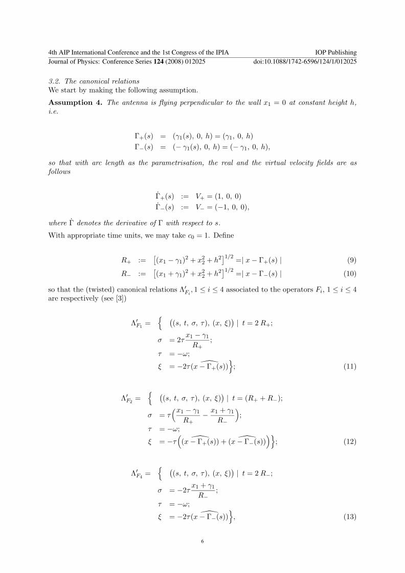
x1 minus γ1

R+minus

x1 + γ1

Rminus= p (17)



x22 =

( t2

4minus γ2

1 minus h2)

+(4γ2

1

t2minus 1

)

x21 (19)



+ (20)


x1 =t

4γ1

(

t minus 2R+

)

(21)


R2+ minus tR+ +

α

4= 0 (22)

with

α =t(t2 minus 4γ2

1)

(t + pγ1) (23)



2



2 (24)



4γ1 (25)





8


i Λprime

F lowast

jfor i 6= j in


σ1 =2τ

c0

x1 minus γ1

R+(27)

σ2 = σ3 =τ

c0

(x1 minus γ1

R+minus

x1 + γ1

Rminus

)

(28)

σ4 = minus2τ

c0

x1 + γ1

Rminus (29)

Notice that

σ1 |x1=0= σ2 |x1=0= σ3 |x1=0= σ4 |x1=0= minus2τ

c0

γ1

R+ |x1=0lt 0

and

limx1rarrinfin

σ1(x) =2τ

c0 lim




2τ

c0

Moreover

partx1R+ = Rminus1

+ (x1 minus γ1) (30)


minus (x1 + γ1) (31)

and

partx1σ1 =

2τ

c0


R2+

=2τ

c0


2

R3+

(32)

partx1σ2 = partx1

σ3 =τ

c0


R2+

minusR2


R3+

=τ

c0

(x22 + h2)(R3

minus minus R3+)

(R+Rminus)3(33)

partx1σ4 =

2τ

c0


R2minus

= minus2τ

c0


2

R3minus

(34)







9

-1

-08

-06

-04

-02

0

02

04

06

08

1

0 100 200 300 400 500

sigm

a

x

h=50

sigma1sigma2sigma4


-1

-08

-06

-04

-02

0

02

04

06

08

1

0 100 200 300 400 500

sigm

a

x

h=100

sigma1sigma2sigma4




1ΛF2


2ΛF1


2z1 minus γ1

Rz+

=

(

x1 minus γ1

Rx+

minusx1 + γ1

Rxminus

)

(35)


Rx+ + Rx

minus = t (36)

2Rz+ = t (37)


+




+)(z1 minus γ1) (38)


z1 =[

(


+

)

γ1 +(

2tRx+ minus t2

)

x1

]

4((Rx+)2 minus tRx

+) (39)


z1 =

(

t2 minus α

4γ1α

)

(

t2 minus 4γ21

)

(40)



10

z1 minus x1 =[


]

α (41)


(

(

x ξ)

(

z ζ)

)

isin ΛF lowast

1 ΛF2

(or similarly(

(

z ζ)

(

x ξ)

)

isin ΛF lowast

2 ΛF1





Acknowledgments












11


i Λprime

F lowast

jfor i 6= j in


σ1 =2τ

c0

x1 minus γ1

R+(27)

σ2 = σ3 =τ

c0

(x1 minus γ1

R+minus

x1 + γ1

Rminus

)

(28)

σ4 = minus2τ

c0

x1 + γ1

Rminus (29)

Notice that

σ1 |x1=0= σ2 |x1=0= σ3 |x1=0= σ4 |x1=0= minus2τ

c0

γ1

R+ |x1=0lt 0

and

limx1rarrinfin

σ1(x) =2τ

c0 lim




2τ

c0

Moreover

partx1R+ = Rminus1

+ (x1 minus γ1) (30)


minus (x1 + γ1) (31)

and

partx1σ1 =

2τ

c0


R2+

=2τ

c0


2

R3+

(32)

partx1σ2 = partx1

σ3 =τ

c0


R2+

minusR2


R3+

=τ

c0

(x22 + h2)(R3

minus minus R3+)

(R+Rminus)3(33)

partx1σ4 =

2τ

c0


R2minus

= minus2τ

c0


2

R3minus

(34)







9

-1

-08

-06

-04

-02

0

02

04

06

08

1

0 100 200 300 400 500

sigm

a

x

h=50

sigma1sigma2sigma4


-1

-08

-06

-04

-02

0

02

04

06

08

1

0 100 200 300 400 500

sigm

a

x

h=100

sigma1sigma2sigma4




1ΛF2


2ΛF1


2z1 minus γ1

Rz+

=

(

x1 minus γ1

Rx+

minusx1 + γ1

Rxminus

)

(35)


Rx+ + Rx

minus = t (36)

2Rz+ = t (37)


+




+)(z1 minus γ1) (38)


z1 =[

(


+

)

γ1 +(

2tRx+ minus t2

)

x1

]

4((Rx+)2 minus tRx

+) (39)


z1 =

(

t2 minus α

4γ1α

)

(

t2 minus 4γ21

)

(40)



10

z1 minus x1 =[


]

α (41)


(

(

x ξ)

(

z ζ)

)

isin ΛF lowast

1 ΛF2

(or similarly(

(

z ζ)

(

x ξ)

)

isin ΛF lowast

2 ΛF1





Acknowledgments












11

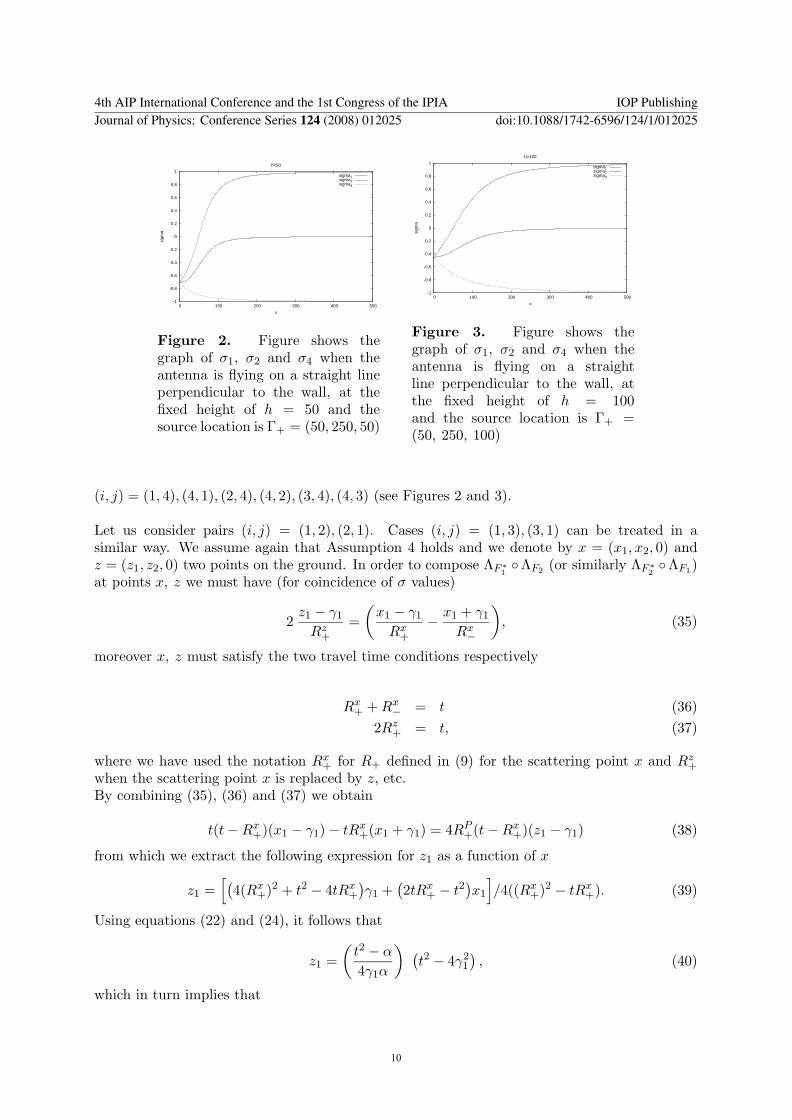
-1

-08

-06

-04

-02

0

02

04

06

08

1

0 100 200 300 400 500

sigm

a

x

h=50

sigma1sigma2sigma4


-1

-08

-06

-04

-02

0

02

04

06

08

1

0 100 200 300 400 500

sigm

a

x

h=100

sigma1sigma2sigma4




1ΛF2


2ΛF1


2z1 minus γ1

Rz+

=

(

x1 minus γ1

Rx+

minusx1 + γ1

Rxminus

)

(35)


Rx+ + Rx

minus = t (36)

2Rz+ = t (37)


+




+)(z1 minus γ1) (38)


z1 =[

(


+

)

γ1 +(

2tRx+ minus t2

)

x1

]

4((Rx+)2 minus tRx

+) (39)


z1 =

(

t2 minus α

4γ1α

)

(

t2 minus 4γ21

)

(40)



10

z1 minus x1 =[


]

α (41)


(

(

x ξ)

(

z ζ)

)

isin ΛF lowast

1 ΛF2

(or similarly(

(

z ζ)

(

x ξ)

)

isin ΛF lowast

2 ΛF1





Acknowledgments












11

z1 minus x1 =[


]

α (41)


(

(

x ξ)

(

z ζ)

)

isin ΛF lowast

1 ΛF2

(or similarly(

(

z ζ)

(

x ξ)

)

isin ΛF lowast

2 ΛF1





Acknowledgments












11

Microlocal analysis of synthetic aperture radar imaging in

Documents

Transcript of Microlocal analysis of synthetic aperture radar imaging in