Microequity for microenterprises - theigc.org · Final report Microequity for ... Results reveal...
67
Final report Microequity for microenterprises Evidence from an artefactual field experiment and survey in Pakistan Muhammad Meki March 2018 When citing this paper, please use the title and the following reference number: F-89306-PAK-1
Transcript of Microequity for microenterprises - theigc.org · Final report Microequity for ... Results reveal...

Final report
Microequity for microenterprises
Evidence from an artefactual field experiment and survey in Pakistan
Muhammad Meki
March 2018 When citing this paper, please use the title and the followingreference number:F-89306-PAK-1
Microequity for Microenterprises: Evidence from an Artefactual
Field Experiment and Survey in Pakistan
Muhammad Meki*
Abstract
Access to finance is often listed as one of the most important constraints on the expansion of small
firms in low-income countries. However, several recent studies reveal that most microcredit-funded
businesses rarely grow beyond subsistence-level entrepreneurship. Other evidence shows that cash and
capital grants have delivered high returns to some microenterprises, and that small changes to contract
structure can have a long-term effect on investment and profits. In this paper, I investigate the potential of
‘microequity’ contracts, which can be viewed as lying at some point on a spectrum between credit and
grants, and provide a more flexible form of capital with performance-contingent repayments and a greater
sharing of risk and reward. I present results from work with two of the largest microfinance institutions in
Pakistan to investigate the effects of microequity contracts on microenterprises. In the first part of the
paper, I describe an artefactual field experiment, designed using a simple model of investment choice
under different financial contracts. This is tested with microenterprise owners who are part of a related
field experiment that provides them with shared-ownership financing to expand their business. Results
reveal that equity-financed microenterprise owners chose investment options with a greater expected
profit than those under debt financing, with heterogeneity analysis suggesting a larger effect for more
risk- and loss-averse individuals. Given the potential benefits, in the second part of the paper I present
results from a field survey to provide insights on the reasons why most microfinance institutions do not
actually offer microequity products. Results reveal the practical implementation challenges related to
costly state verification, adverse selection into income-sharing contracts and moral hazard caused by
inappropriately-tailored profit-sharing ratios.
*DPhil (PhD) Candidate in Economics, University of Oxford. Email: [email protected]. I acknowledgefunding from the International Growth Centre (IGC). This project would not have been possible without the generous support of DrAmjad Saqib and Shahzad Akram of Akhuwat, Dr Rashid Bajwa and Tahir Waqar at National Rural Support Programme (NRSP),and Simon Quinn, Colin Mayer, Kashif Malik, and Ahmad Ayub.
1

Introduction
1 Introduction
Access to finance is often listed as one of the most important constraints on the expansion of informal micro,
small and medium enterprises in many low-income countries.1 Many existing studies focus on the role
of microcredit as a source of capital; other work complements this by considering the potential effect of
microsavings and microinsurance. In this paper, I consider a different approach: ‘microequity’. Microe-
quity contracts, which involve performance-contingent repayments, have the potential to provide a more
flexible form of capital that could more effectively stimulate growth for some microenterprise in developing
countries. Microequity contracts may, relative to microcredit contracts, encourage higher risk and higher
return investments, by providing a form of implicit insurance to microenterprises that automatically reduces
repayment requirements when business conditions are challenging. This is in comparison to microcredit and
microsavings products, which often have strict payment schedules (and, in the case of microcredit, relatively
high interest rates). The effects could be particularly strong for microenterprise owners whose behavioural
characteristics lead them to under-invest in profitable opportunities, such as those with higher levels of
risk- and loss-aversion. Such individuals may be more willing to choose riskier but higher expected-return
investments when provided with the implicit insurance of microequity contracts, which mitigate the risk of
losing their own wealth, compared to non-performance-contingent, fixed-repayment debt contracts. Microe-
quity contracts also have the potential to serve hundreds of millions of low-income microentrepreneurs from
the world’s population of 1.6 billion Muslims, many of whom remain unbanked both by microcredit and
microsavings products because of the religious prohibition on interest.
Initially, it was believed that microcredit would be an effective tool for encouraging entrepreneurship and
growth of microenterprises. However, several recent studies have suggested that microloans have not had
large benefits for most entrepreneurs and that microcredit-funded businesses rarely grow beyond a subsistence
level of entrepreneurship. Banerjee, Karlan, and Zinman (2015) report on seven randomised evaluations of
microcredit, using a variety of sampling, data collection, experimental design, and econometric strategies1 See Ayyagari, Beck, and Demirguc-Kunt (2007); Beck, Demirgüç-Kunt, and Martinez Peria (2008); Stein, Ardic, and Hommes
(2013).
2

Introduction
to identify causal effects of expanded access to microcredit on borrowers or communities.2 They consis-
tently find no transformative impact from microcredit. In particular, take-up rates were unexpectedly low,
investments rarely resulted in increased profits, and none of the studies found a significant impact on average
household income. Among several recommendations, Banerjee, Karlan, and Zinman (2015) identify the
following key challenges for the next generation of microfinance studies: (i) investigating how innovations
to microfinance contract structure can improve take-up rates and effectiveness; (ii) addressing the limited
evidence on repeat borrowers; and (iii) broadening our understanding of non-credit microfinance activities. In
this paper, I aim to contribute to these objectives by investigating the viability of microequity contracts, which
provide a more flexible form of capital with performance-contingent repayments and a greater sharing of
risk and reward, using an artefactual field experiment and a field survey with two of the largest microfinance
institutions in Pakistan.
Standard microcredit contracts are often characterised by high interest rates and immediate repayment re-
quirements. While the majority of the results from the literature on microcredit have showed little effect from
standard microcredit products on the growth of microenterprises, recent evidence reveals that small changes
to contract structure, such as repayment grace periods, can have a long-term effect on profits and facilitation
of lumpy investment.3 Further, cash and capital grants have delivered high and sustained returns to at least
some kinds of microenterprise.4 Microequity contracts can be viewed as lying at some point on a spectrum
between credit and grants, sharing characteristics of both, by providing capital with performance-contingent
repayments.
This paper draws on the work of Fischer (2013), who uses theory and a ‘lab-in-field’ experiment to investigate
the possibility that the structure of many existing microfinance contracts discourages risky but high-expected-
return investments, with a particular focus on the difference between individual- and joint-liability microcredit2 See Augsburg, De Haas, Harmgart, and Meghir (2015); Tarozzi, Desai, and Johnson (2015); Duflo, Banerjee, Glennerster, and
Kinnan (2013); Angelucci, Karlan, and Zinman (2015); Attanasio, Augsburg, De Haas, Fitzsimons, and Harmgart (2015); Crépon,Devoto, Duflo, and Parienté (2015); Karlan and Zinman (2011). Meager (2018) jointly estimates the average effect and theheterogeneity in effects across these seven studies using a Bayesian hierarchial model, and finds support for the conclusion thatthe average effect on household outcomes is close to zero, while there is some evidence of a positive effect for households withprevious business experience.
3 See Field, Pande, Papp, and Rigol (2013); Battaglia, Gulesci, and Madestam (2017); Barboni (2017).4 See De Mel, McKenzie, and Woodruff (2008); Fafchamps, McKenzie, Quinn, and Woodruff (2014).
3

Introduction
contracts on risk-sharing and informal transfers between pairs of individuals who have been issued a loan. He
also investigates the effect of a quasi-equity contract, in which partners who are given a loan also have profit-
and loss-sharing enforced on them, and finds that this contract led to increased risk-taking and expected
returns relative to all other contracts (both individual- and joint-liability debt contracts), and actually produced
the lowest default rates.5
There are over 1.6 billion Muslims in the world, representing nearly a quarter of the global population.
The religious prohibition on usury (‘riba’) means that many Muslim microentrepreneurs remain unbanked
both by microcredit and microsaving products.6 An equity-based product, though not restricted to any
one particular religion or group, has the potential to meet the demands of hundreds of millions of poor
Muslims, many of whom reject conventional loan products on religious grounds.7 Research from the Islamic
Development Bank reports that that in the six countries with the largest Muslim populations (Indonesia, India,
Pakistan, Bangladesh, Egypt and Nigeria) the number of people living on less than $2 per day far exceeds
half a billion.8 Financial exclusion rates in India are as high as 80% for Muslims, compared to 20% for
non-Muslims.9 Recent reports by the World Bank and IMF discuss the benefits of risk-sharing products and
call for innovations in equity-based contracts for micro-, small- and medium-sized enterprises.10
In the first part of the paper, I test a microequity contract using an artefactual field experiment, with mi-
croenterprise owners who were part of a broader field experiment, two-thirds of whom were randomly
offered a relatively large amount of financing to purchase an asset for their business (using an ‘equity-like’,
shared-ownership contract). The sample consists of growth-oriented microenterprise owners who had suc-
cessfully graduated from previous loan cycles, reaching the upper limit of borrowing of $500 from Akhuwat,5 The major differences between this paper and Fischer (2013) are that Fischer’s equity-like contract is itself a hybrid of a debt
and equity contract that was implemented with participants in pairs, with the primary aim of studying informal risk sharing andtransfers between these pairs of individuals. Other major differences include the characteristics of the sample: Fischer usesonly females with relatively low incomes, and it is not clear how many of them were managing a business. In my context, allparticipants were growth-oriented microenterprise owners who had successfully graduated from previous loan cycles, reaching theupper limit of borrowing of $500, and had entered into an experiment that provided them with financing up to the value of $2,000to expand their business with the purchase of a fixed asset using a shared-ownership contract.
6 See El-Gamal, El-Komi, Karlan, and Osman (2014).7 See Nimrah, Michael, and Xavier (2008).8 See Obaidullah and Khan (2008).9 See El-Komi and Croson (2013).
10 See World Bank (2012); Kammer, Norat, Pinon, Prasad, Towe, and Zeidane (2015).
4

Introduction
one of the largest microfinance institutions in Pakistan, and who had expressed an interest in expanding
their business by purchasing a fixed asset up to the value of $2,000. As such, this experiment has greater
external validity compared to most ‘lab-in-the-field’ studies because all participants are actual microenterprise
owners making an important investment decision for their business. The experiment was designed based
on a simple theoretical model, in which a utility-maximising agent makes investment decisions in discrete
time. Financial contracts are then introduced to investigate investment behaviour under equity and debt. The
model predicts that agents are more likely to choose higher-risk, higher expected-return investment options
when financed with performance-contingent-repayment equity contracts, compared to investment decisions
taken under a fixed-repayment debt contract. This prediction is stronger for more risk-averse agents. I demon-
strate the robustness of these predictions to changes in the parameters of the model, which is then tested
using the artefactual field experiment with microenterprise owners. Results from the experiment reveal that
equity-financed microentrepreneurs chose investment options with a higher expected return than under debt
financing, with an effect size of 0.40 standard deviations. Heterogeneity analysis with pre-specified variables
reveals a treatment effect that is approximately 50% larger for the most risk- and loss-averse microenterprise
owners. Such individuals may under-invest in profitable opportunities due to their aversion to risk and losses;
microequity contracts have the potential to stimulate profitable but more risky investment choices for this
group of individuals through the implicit insurance inherent in performance-contingent repayments. However,
while the welfare effects on this population of individuals could be significant, from a policy perspective
microfinance institutions may not wish to provide such financing if those individuals who take the most
risk under equity financing also tend to be those with the worst business management practices, education
or cognitive ability. The results presented in the second part of the heterogeneity analysis help to mitigate
such concerns: I find no evidence that microenterprise owners with lower business management practices,
education or cognitive ability are those for whom equity contracts incentivise the greatest risk-taking relative
to debt. In fact, there is evidence of the opposite effect, with the greatest impact from equity contracts on
those with the highest business practices, education and cognitive ability.
Following on from the positive results from the artefactual field experiment, the second part of the paper
provides some insights for why large microfinance institutions (MFIs) do not typically offer microequity
5

Introduction
contracts alongside other products in their portfolios. Given the stated objectives of many microfinance
institutions to consider borrower welfare as well as profits, it seems surprising that no large microfinance
institution appears to be implementing microequity contracts, given the potential benefits, in particular
for individuals whose risk- and loss-aversion may lead them to under-invest, and given the evidence that
those individuals are not characterised by the lowest levels of business management practices, education or
cognitive ability. To investigate this, I report on an attempt by the National Rural Support Program (NRSP),
another one of the largest microfinance institutions in Pakistan, to implement microequity contracts with
microenterprise owners in the field. Results from a detailed client survey and a post-survey focus group
with senior management reveal the significant challenges of implementing equity-based contracts within a
conventional microcredit organisation. I find that, while contracts were initially implemented with profit- and
loss-sharing, gradually clients and loan officers abandoned the performance-contingent payment features
and converged back to a model of fixed-repayment debt contracts. Interviews with senior management and
loan officers uncover reveal key reasons for this convergence, which echo results from theoretical work
that has investigated the difficulties in implementing performance-contingent contracts, such as equity or
sharecropping, due to costly state verification, adverse selection and moral hazard.11
The second part of this paper reveals two major insights. First, from the supply-side, the main challenge of
implementing equity-like contracts was related to the organisational structure of a conventional microfinance
institution: specifically, how loan officers are incentivised. Loan officers in the study reported that they
were familiar with disbursing a relatively high volume of loans and focusing the majority of their efforts
on maximising the repayment rate of their loan portfolio, based on which they are paid a bonus.12 Loan
officers did not have much incentive to finance higher-return, higher-risk microentrepreneurs by providing
them with a product that contained possible loss-sharing, especially because the loan officer would not
themselves benefit from the upside portion of the entrepreneur’s payment. Further, loan officers reported
that it took much added effort to monitor microenterprises and their profits and losses, on which they had
to calculate shared payments. These results provide some support for the theoretical result of Townsend11 See Townsend (1979); Stiglitz and Weiss (1981).12 Note that this could also lead to an incentive to re-finance the loan of a client who is performing poorly, rather than investigating
whether their business is worthy of being re-financed.
6
Introduction
(1979), who shows that under costly state verification the optimal financing mechanism is a standard debt con-
tract, rather than performance-linked contracts that require the capital provider to monitor the microenterprise.
The second major insight relates to the incentives of microfinance clients themselves in the implementation of
profit-sharing contracts. Results from the survey and interviews illustrate that many microenterprise owners
had serious objections to the profit-sharing rule used in the contracts when they were originally implemented.
A common sharing rule of 20-80 was applied by the MFI – where the microenterprise shared 20% of its
monthly profits – but this led to the most profitable microentrepreneurs having to share too much of their
profits and thus the equity product, ironically, appeared to them to be very ‘inequitable’. Once again, it was
beyond the remit and incentives of loan officers to spend a large amount of time auditing the accounts of the
microenterprise and carefully tailoring the sharing ratio based on expected profits and losses of the business
after the capital injection. Over time, loan officers and clients mutually agreed to remove the performance-
contingent aspect of the contracts, which converged to a fixed repayment schedule. Had NRSP maintained
performance-contingent contracts alongside fixed-repayment contracts, a serious problem of adverse selection
may have developed, with the most profitable microenterprises deciding to re-negotiate to a debt contract,
and the least profitable ones remaining on performance-contingent contracts. Hence, the decision taken by
NRSP management to revert all contracts back to a standard fixed repayment schedule appears to have been
appropriate. This decision to move back to debt-like contracts also appears prudent in light of the potential
adverse consequences of moral hazard. Since a 20-80 sharing ratio was considered inappropriate by some
of the more profitable businesses, in that they were obliged to share too much of their profits, had NRSP
not renegotiated the contract then it could have created negative incentives for those microenterprises stuck
on ‘unfair’ sharing ratios. This may have encouraged them either to exert less effort – for instance if they
equated their marginal disutility of effort with their share of their marginal product rather than total marginal
product – or to simply understate their profits, which would be difficult to detect due to costly state verification.
Intriguingly, NRSP branch managers also observed that, even though the contracts originally maintained a
‘downside option’ that did allow for loss-sharing ex-ante, in practice no entrepreneurs ever exercised this
loss-sharing option. This was due to a fear that if they did not meet their expected payment every month, it
7

A simple model of contract structure and investment choice
would adversely affect their standing with the bank, which may hinder their ability to borrow in the future.
Therefore, fears regarding reputation and dynamic incentives actually led to microenterprise owners not
exercising their loss-sharing option, even when NRSP had explicitly allowed it. In summary, these findings
from the survey of NRSP clients suggest that it is very challenging to implement equity-based contracts
within a conventional microcredit organisation. The major constraints relate to the incentives of microcredit
loan officers and those of clients, as discussed in earlier theoretical work on optimal financial contracts in
the presence of asymmetric information and costly state verification. These are compounded by the related
problems of adverse selection (the most profitable microenterprises selecting out of equity contracts) and
moral hazard (distortionary effects caused by inappropriately chosen income-sharing ratios).
The remainder of the paper proceeds as follows. In Section 2, I outline the simple model that was used to
design the artefactual field experiment, which is described in Section 3, and for which results are presented in
Section 4. Section 5 presents results from the field survey of NRSP clients, and Section 6 concludes.
2 A simple model of contract structure and investment choice
2.1 General setup
In this section, I outline a simple model in which an agent makes a series of investment decisions in discrete
time. I describe the general setup of the model, how financial contracts are introduced (debt and equity),
and the model’s predictions for the behaviour of agents under the financial contract ‘treatments’. The model
forecasts that agents are more likely to choose investment options with a higher expected return (and higher
risk) when financed with the equity contract, compared to the debt contract. This prediction is stronger for
more risk-averse agents. I demonstrate the robustness of these predictions to changes in the structure of the
model. This model is then used to design the experiment that is outlined in Section 3, which is implemented
with microenterprise owners who are part of a large field experiment, in order to test the effect of financial
contracts on investment choice.
In the model, the agent begins the game with initial wealth w1, and makes an investment choice in each
8

2.1 General setup
decision round. There are T decision rounds; in each round the agent chooses from a set of j investment
options, with each investment option having: (i) a good outcome gj ; (ii) a bad outcome bj . The bad outcome
always has a payoff of zero (bj = 0), while the good outcome has some positive payoff (gj > 0). Each
outcome is equally likely. I define a payoff matrix with each row corresponding to one of the j investment
options pairs (bj , gj). Each of the j investment options also has an associated cost, cj . The agent chooses
investment options that maximise their expected utility, subject to the constraint that their current wealth
is sufficient to pay for the chosen investment option. The agent is assumed to have a constant relative
risk-aversion (CRRA) utility function over wealth wt:
u(wT ) =w1−rT − 1
1− r(1)
where r is the coefficient of relative risk-aversion (CRRA) (and u(wt) = lnwt if r = 1). Backward induction
is used to solve the model for the optimal decisions of the agent. I begin by defining a ‘wealth grid’ at the
terminal period T, with [wT,1, wT,2, ..., wT,MAX ] representing gradually increasing values on the discretised
state space for wealth, and wT,MAX the maximum possible wealth at T .13 Similarly, wealth grids are created
for all periods t = 1, 2, ..., T − 1. A ‘value grid’ is then created for each period t, where each point on the
value grid represents the utility from the corresponding point on the wealth grid at time t, based on the utility
function in equation 1: [u(wt,1), u(wt,2), ..., u(wt,max)]. This therefore represents a discrete choice dynamic
programming problem with wealth wt as the state variable and the investment decision as the choice variable.
The objective is to fill in each of these value grids, starting from the last period, and working back one period
at a time. The model is solved by backward induction; in the final period T , the agent chooses the investment
option that maximises their expected utility. This optimal choice of investment option is computed for every
possible starting wealth level on the T − 1 wealth grid, which leads to a vector of optimal investment choices,
for each possible wealth level wT−1. This is then repeated for the T − 2 wealth grid, and so on, until period
t = 1. This provides an optimal solution grid for each agent, based on their CRRA parameter r. Having
solved the model backwards, it is then possible to ‘simulate forwards’ in order to generate predictions for
investment choices made by agents with different levels of risk-aversion, which is outlined in Sections 2.3
and 2.4.13 Calculated as the number of previous rounds (T − 1) multiplied by the maximum payoff from the set of j investment options (gj).
9

2.2 Adding financial contracts
2.2 Adding financial contracts
Each game is played under a different financial contract environment, described below, which affects the
amount of capital with which the agent begins and the terminal payoffs at the end of the game. These different
environments correspond to the ‘treatment arms’ in the experiment described in Section 3:
Control Treatment (CT): The control treatment is the baseline scenario, upon which different financial
contract treatments are added. In the general setup, an agent begins period t = 1 with initial capital w1.
The agent can then choose any of the affordable j investment options; in period t = 1, they can afford any
investment option with cost cj ≤ w1. The agent selects the optimal investment option and pays the cost.
The outcome of the investment option is then realised, with the agent carrying forward to the next round
their initial wealth w1, minus the cost of the investment option that they chose cj , plus the payoff from the
investment option that they chose (bj or gj , with equal likelihood). The game proceeds in the same manner
for T rounds, after which it ends and the agent keeps whatever wealth is remaining.
Debt Treatment (DT): In the debt dreatment, the agent begins with the same initial capital w1 as in the
control treatment, but they also receive an additional amount of capital k in the form of a zero-interest loan
(the debt contract with which the microenterprise owners in the experiment are most familiar).14 At the end
of the T rounds, the loan of k must be repaid in full. The main purpose of the debt treatment is that it mimics
‘external financing’ that is required by the agent to invest in higher expected-return investment options, which
also cost more, and which the agent cannot afford when their initial wealth level is w1 (as in the control
treatment).
Equity Treatment, 50-50 Sharing (ET1): In the first equity treatment, the agent also begins with w1 and
an additional amount of capital k. However, the additional capital k is now given in the form of equity-based
financing. The equity capital does not have a fixed repayment obligation at the end of the game, which is the
requirement of the loan in debt treatment. Instead, there is a requirement to share all the wealth that is left
at the end of the game in a 50-50 ratio (the agent keeps 50% of the remaining wealth, and shares 50%; this
includes the initial wealth w1 that they were given as starting capital).14 The MFI partner in this artefactual field experiment and the larger field experiment, Akhuwat, predominantly lends at zero interest.
10
2.3 Model Predictions
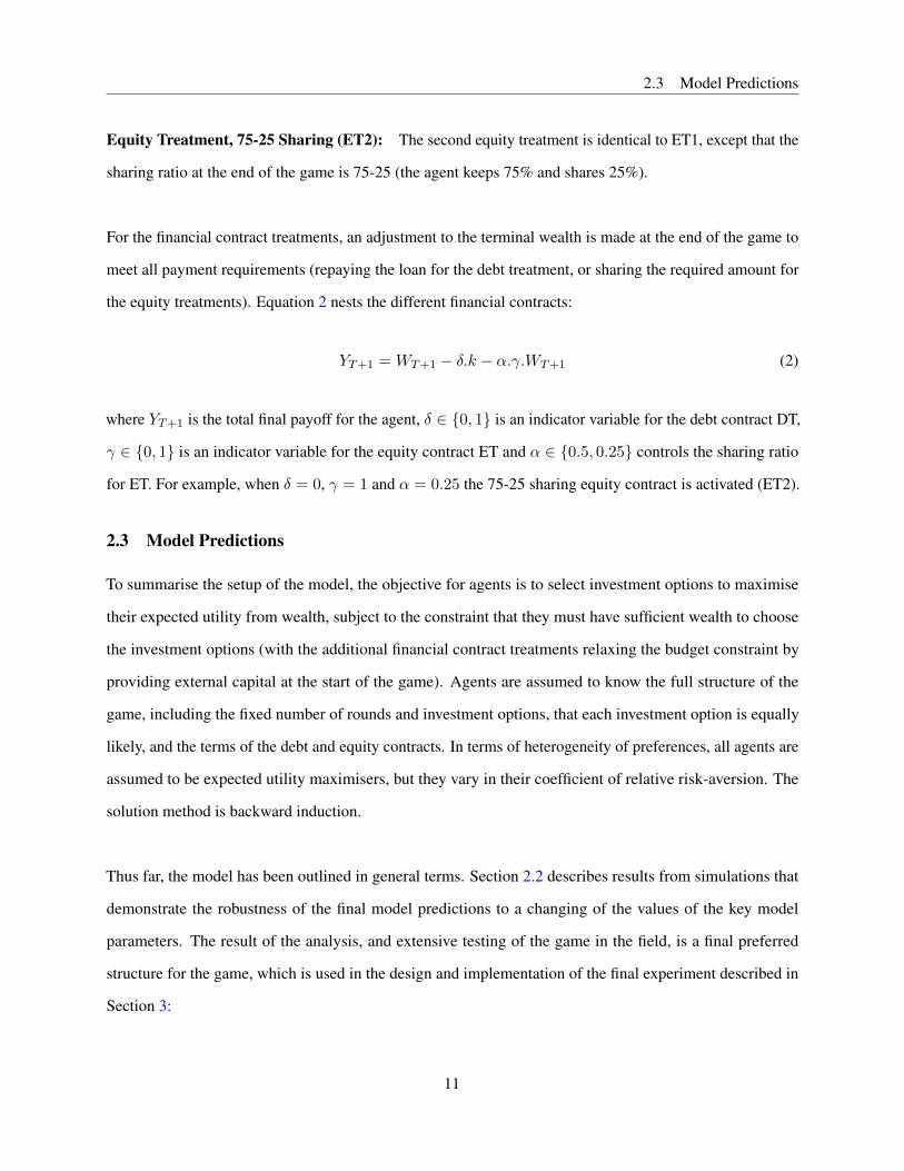
Equity Treatment, 75-25 Sharing (ET2): The second equity treatment is identical to ET1, except that the
sharing ratio at the end of the game is 75-25 (the agent keeps 75% and shares 25%).
For the financial contract treatments, an adjustment to the terminal wealth is made at the end of the game to
meet all payment requirements (repaying the loan for the debt treatment, or sharing the required amount for
the equity treatments). Equation 2 nests the different financial contracts:
YT+1 =WT+1 − δ.k − α.γ.WT+1 (2)
where YT+1 is the total final payoff for the agent, δ ∈ {0, 1} is an indicator variable for the debt contract DT,
γ ∈ {0, 1} is an indicator variable for the equity contract ET and α ∈ {0.5, 0.25} controls the sharing ratio
for ET. For example, when δ = 0, γ = 1 and α = 0.25 the 75-25 sharing equity contract is activated (ET2).
2.3 Model Predictions
To summarise the setup of the model, the objective for agents is to select investment options to maximise
their expected utility from wealth, subject to the constraint that they must have sufficient wealth to choose
the investment options (with the additional financial contract treatments relaxing the budget constraint by
providing external capital at the start of the game). Agents are assumed to know the full structure of the
game, including the fixed number of rounds and investment options, that each investment option is equally
likely, and the terms of the debt and equity contracts. In terms of heterogeneity of preferences, all agents are
assumed to be expected utility maximisers, but they vary in their coefficient of relative risk-aversion. The
solution method is backward induction.
Thus far, the model has been outlined in general terms. Section 2.2 describes results from simulations that
demonstrate the robustness of the final model predictions to a changing of the values of the key model
parameters. The result of the analysis, and extensive testing of the game in the field, is a final preferred
structure for the game, which is used in the design and implementation of the final experiment described in
Section 3:
11

2.3 Model Predictions
(i) Two rounds in the game;
(ii) Initial capital w1 of 200 and external capital k of 500;
(iii) Five investment options (monotonically increasing in risk-return, as illustrated in Figure 1).
Figure 1: Investment options
Note: Each row represents one of the five possible investment options, along with thecost of each option and the payoff in each of the two possible states. The expectedpayoff and the expected payoff net of cost are also displayed, but were not shown tothe participant in the final activity.
The final model predictions can be summarised as:
Hypothesis 1 In general, agents take more risk under equity financing.
Hypothesis 2 More risk-averse agents take more risk under equity financing.
Figure 2 illustrates the optimal solution grid for the model under the preferred game structure. Each row
represents the optimal investment choice, as solved for in the model, for different values of the CRRA
parameter of the agent. CT, DT, ET1 and ET2 refer to the four different treatments. Each entry is a number
between 1 and 5, representing the choice between the five investment options listed in Figure 1. For each
treatment, there are three columns, which represent:
(i) The optimal investment choice in round 1;
(ii) The optimal investment choice in round 2, if the bad outcome occurred in round 1;
(iii) The optimal investment choice in round 2, if the good outcome occurred in round 1.
12

2.3 Model Predictions
Figure 2: Model solution grid.
Note: Each number represents the optimal investment choice foran agent with a given coefficient of relative risk-aversion (CRRA)and under a given treatment environment.
As can be seen in Figure 2, the optimal solution implies greater risk-taking in the equity treatments, ET1 and
ET2, than the debt treatment DT. This is reflected in Figure 3, which illustrates results from simulations of the
model, pooling together the two equity treatments. Each point represents the coefficient from a regression of
the expected return of the investment options chosen by an agent with a given CRRA parameter on treatment
indicator variables (an OLS regression without a constant). The top two panels illustrate simulated results
for the investment decisions made in the first round and second round respectively, with the bottom panel
displaying the sum of the two decision rounds. In each round, it can be observed that a risk-neutral agent
takes the same amount of risk under both debt and equity contracts, but for agents with CRRA parameters
above 0.5 there is relatively less risk-taking under debt contracts. The gap between risk-taking under equity
and debt is largest in the intermediate range of illustrated CRRA parameters, while the effect for the most
risk-averse people is relatively smaller but still positive in the direction of greater risk-taking under equity.
13

2.4 Robustness simulations
Figure 3: Simulated results
Note: The grey dotted line plots the risk-taking under equity minus risk-taking under debt. Simulations were done in MATLAB witha simulated sample of size 300 and 300 simulations, with regressions being run for each simulated dataset. Results are also stableand similar for a lower number of simulations and smaller sample size.
2.4 Robustness simulations
Figures 15 - 19 of the Appendix illustrate results from a number of simulations, which reveal the robustness
of the model’s predictions to changes in key parameters. Each simulation is done with results compared to the
‘baseline’ specification that was implemented in the final experiment: two decision rounds, five investment
options to choose from each round, starting capital of 200 and additional capital of 500 for the financing
contracts.
Number of decision rounds: Figure 15 presents simulated results when the number of decision rounds in
the game is changed from two to three, five, seven and ten. Results are qualitatively the same, and based on
14

2.4 Robustness simulations
logistical reasons and a desire not to over-burden participants, the final design included only two rounds.
Number of investment options: Figure 16 illustrates results using three, seven and ten investment options
respectively. Again, predictions do not qualitatively change. Based on piloting, it was decided that five
investment options provided the optimal trade-off between client comprehension and offering sufficient
variation in choices.
Initial wealth level: In Figure 17, the initial level of starting capital w1 was sequentially increased. While
results reveal the same pattern of equity-financed agents taking more risk than debt-financed agents, with
the effect positive for more risk-averse agents (before tailing off for the most risk-averse agents), the CRRA
region in which the effect is largest shifts to the right as the initial wealth level is increased. This is an
intuitive result, given that the assumed utility function exhibits constant relative risk-aversion (CRRA), which
implies decreasing absolute risk-aversion (DARA), such that an agent who experienced an increase in wealth
should increase their absolute level of risk-taking. Although not illustrated in Figure 17, when comparing
risk-taking for each of the two treatment contracts relative to the control group, who do not get access to
the additional capital of 500, it can be seen that the effect is smaller as the initial wealth level is increased.
Again, this is quite an intuitive result, as less ‘value’ is added by the external capital treatments when the
agent begins in a wealthier state. Nonetheless, the overall effect of greater risk-taking under equity than debt
persists, with the difference increasing in risk-aversion up to a certain CRRA coefficient where it begins to
decrease but remains positive.
Amount of external capital: Figure 18 illustrates simulated results for different values of the external
capital amount k. Results remain qualitatively similar, although the effect size when the external capital
amount is smallest decreases, as would be expected. It should be noted that there are potentially large
differences in the welfare implications of the two financial contracts. For example, if the external capital
amount is very low, the equity contracts begin to look rather ‘unequal’, since agents are provided with very
little capital yet they are required to share a large amount of the firm’s value at the end of the game.
Finally, Figure 19 presents simulations of the terminal wealth at the end of the game for the two treatments.
15

Experimental implementation
Results show that the equity contracts are not unambiguously ‘better’ than the debt contracts in terms of
expected terminal wealth; in particular, for risk-neutral agents and those with a CRRA coefficient up to 0.5,
expected terminal wealth is the same under both debt and equity contracts. For higher levels of risk-aversion,
equity-financed entrepreneurs do end with higher terminal wealth, as would be expected given the observed
greater risk-taking.
3 Experimental implementation
In this section, I describe the setup of the artefactual field experiment, which was designed to test the
predictions of the model set out in Section 2, and to coincide with a broader field experiment conducted
with growth-oriented clients of the fastest growing microfinance institutions in Pakistan to help them finance
business expansion. Akhuwat is based in Lahore and operates in 708 branches across Pakistan, with 814,101
active borrowers and an outstanding loan portfolio of PKR 11.7 billion (approximately USD 105 million).15
The sample consisted of microenterprise owners who had successfully completed at least one loan cycle
with Akhuwat, and who had expressed an interest in expanding their business by purchasing a fixed asset.
Individuals were invited to a half-day workshop, where a baseline survey was conducted and the new
asset-based microfinance contract was explained to them (after this session, two-thirds of participants were
randomly offered this new contract to finance an asset for their business, up to the value of $2,000). During
the workshop, and after the baseline survey, enumerators conducted a detailed session of behavioural games,
with the microequity game, based on the model in Section 2, as the main activity.
3.1 Summary statistics for microenterprise owners
Table 1 presents summary statistics for the microenterprise owners who participated in the study. 90%
were male, with an average age of 38 and seven years of formal education. 84% were married, and the
average household size was six, of which two people were typically earning some form of income. 62%
of participants were themselves the head of the household, with a further 22% as the son or daughter of
the household head, and 8% as the husband or wife of the head. In terms of business characteristics, the
mean number of businesses in the household was 1.2, with a median of 1. The average number of years of15 Information correct as of 15 December 2017.
16

3.1 Summary statistics for microenterprise owners
experience in that business was 9.6. The mean number of employees was 1.1, with a median of 0. Average
monthly business profits were approximately US$ 253, with a median of $217, and average total fixed assets
were $1,175 (median $395). Average monthly household income from all sources was $560 (median $350),
and average monthly household expenditure was $218 (median $185). The most popular business sector
was rickshaw driving (20%), followed by clothing and footwear production (10%), food and drink sales
(8%), and retail trade in the form of fabric and garment sales (6%). As a comparison to two of the most
prominent studies on microenterprises, average microenterprise profits in De Mel, McKenzie, and Woodruff
(2008) were 3,850 Sri Lankan Rupees (approximately $25 at current market rates) and 125 Ghanaian Cedis
($ 27) in Fafchamps, McKenzie, Quinn, and Woodruff (2014). The average microenterprise owner in this
current study is larger in terms of business profits than the two most prominent microenterprise-focused
studies, which is unsurprising given that the wider field experiment targets growth-oriented microenterprise
owners who had successfully completed previous loans and were looking to finance an asset for business
expansion up to the value of approximately $2000. The seven microcredit field experiments summarised in
Banerjee, Karlan, and Zinman (2015) contained a mixture of microenterprise-targeted products and ones
with no restrictions. The most relevant comparisons would be Tarozzi, Desai, and Johnson (2015), who
worked with a microenterprise-targeted loan product in Ethiopia with an approximate value of $500, Karlan
and Zinman (2011), who offered approximately $220 to microenterprises in the Philippines, and Angelucci,
Karlan, and Zinman (2015), who offered approximately $ 450 to Mexican microenterprises.
Table 1: Akhuwat sample: Summary statistics
Mean SD 10th Pctile Median 90th Pctile Obs.Gender 0.1 0.3 0.0 0.0 0.0 718Age 38.0 10.3 26.0 37.0 52.0 718Education 7.4 3.7 0.0 8.0 12.0 718Married 0.8 0.4 0.0 1.0 1.0 718Household size 6.3 2.8 4.0 6.0 9.0 718Household earners 2.0 1.2 1.0 2.0 4.0 718Number of businesses 1.2 0.6 1.0 1.0 2.0 718Business experience 9.6 8.1 2.0 7.0 20.0 718Number of employees 1.1 3.1 0.0 0.0 3.0 718Monthly profits 25,327.7 18,005.6 7,500.0 21,666.7 48,333.3 718Total fixed assets 117,513.5 310,687.7 0.0 39,500.0 250,000.0 718Household Income 55,967.2 73,649.0 0.0 35,000.0 120,000.0 718Household Expenditure 21,785.4 17,266.5 9,500.0 18,450.0 36,000.0 718
17

3.2 Eliciting risk preferences and loss-aversion
3.2 Eliciting risk preferences and loss-aversion
Microenterprise owners who had expressed an interest in expanding their business with a fixed asset were
invited to a half-day workshop, where a baseline survey was conducted. Prior to the microequity game, be-
havioural games were conducted to measure risk preferences and loss-aversion, in order to provide measures
for the analysis of heterogeneous treatment effects.
The first measure of risk-aversion was survey-based, in which each respondent was asked the following four
questions:16
(i) "How would you rate your willingness to take risks in financial matters?"
(ii) "How would you rate your willingness to take risks in your occupation?"
(iii) "How would you rate your willingness to take risks when it comes to having faith in other people?"
(iv) "How do you see yourself? Are you generally a person who is fully willing to take risks or do you try to
avoid taking risks?"
The questions were adapted from Dohmen, Falk, Huffman, Sunde, Schupp, and Wagner (2011), who used a
large sample to show that responses to the survey-based measure were a reliable predictor of actual risky
behaviour in incentivised risk preference elicitation activities. The authors argue that relatively simple
survey-based measures, compared to often quite complex paid lottery experiments, are easy to use, cheap to
administer, and deliver a behaviourally valid measure of risk attitudes, which maps onto actual choices in risk
preference elicitation activities with real monetary consequences.
I complemented the survey-based measure of risk-aversion with an incentive-compatible measure, using a
method that provided the best trade-off between comprehension and quality of data for this population of16 Responses were given on a scale of 1 to 10, with 0 representing ‘risk-averse’ and 10 for ‘fully prepared to take risks’.
18
3.2 Eliciting risk preferences and loss-aversion
microenterprise owners, as discovered through extensive piloting.17 The final incentivised risk preference
elicitation activity can be characterised as a ‘certainty-equivalent method’.18 Respondents were posed a series
of 30 questions, where they were required to choose between a certain amount of money or an uncertain
investment option, which had two possible outcomes: (i) a ‘bad’ outcome, with a payoff of zero; or (ii) a
‘good’ outcome, with a payoff of PKR 1,000.19
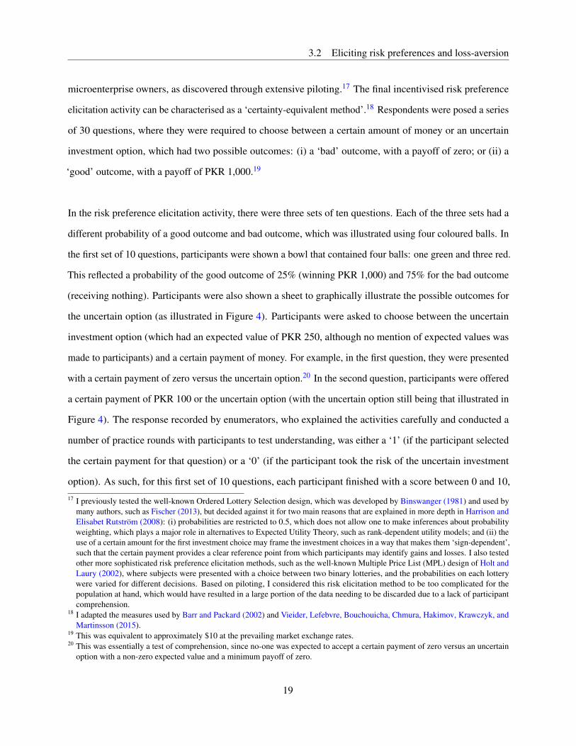
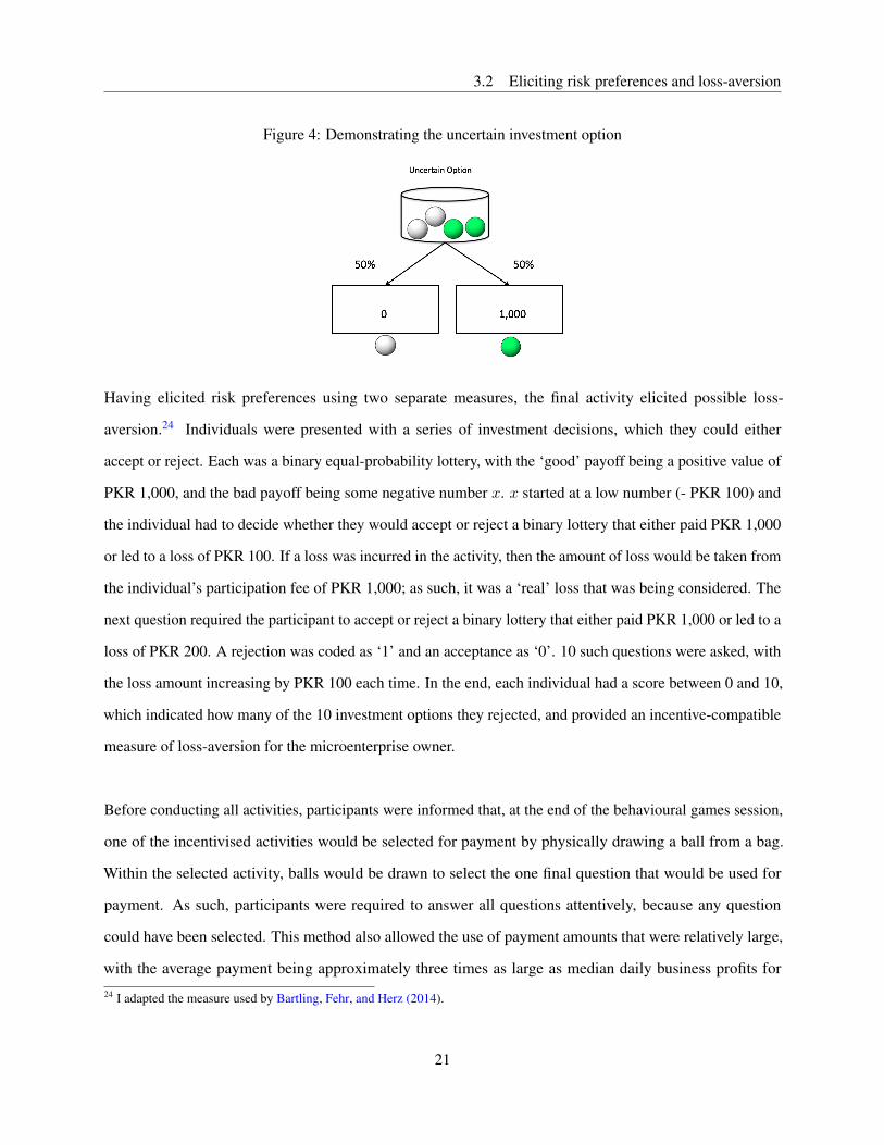
In the risk preference elicitation activity, there were three sets of ten questions. Each of the three sets had a
different probability of a good outcome and bad outcome, which was illustrated using four coloured balls. In
the first set of 10 questions, participants were shown a bowl that contained four balls: one green and three red.
This reflected a probability of the good outcome of 25% (winning PKR 1,000) and 75% for the bad outcome
(receiving nothing). Participants were also shown a sheet to graphically illustrate the possible outcomes for
the uncertain option (as illustrated in Figure 4). Participants were asked to choose between the uncertain
investment option (which had an expected value of PKR 250, although no mention of expected values was
made to participants) and a certain payment of money. For example, in the first question, they were presented
with a certain payment of zero versus the uncertain option.20 In the second question, participants were offered
a certain payment of PKR 100 or the uncertain option (with the uncertain option still being that illustrated in
Figure 4). The response recorded by enumerators, who explained the activities carefully and conducted a
number of practice rounds with participants to test understanding, was either a ‘1’ (if the participant selected
the certain payment for that question) or a ‘0’ (if the participant took the risk of the uncertain investment
option). As such, for this first set of 10 questions, each participant finished with a score between 0 and 10,17 I previously tested the well-known Ordered Lottery Selection design, which was developed by Binswanger (1981) and used by
many authors, such as Fischer (2013), but decided against it for two main reasons that are explained in more depth in Harrison andElisabet Rutström (2008): (i) probabilities are restricted to 0.5, which does not allow one to make inferences about probabilityweighting, which plays a major role in alternatives to Expected Utility Theory, such as rank-dependent utility models; and (ii) theuse of a certain amount for the first investment choice may frame the investment choices in a way that makes them ‘sign-dependent’,such that the certain payment provides a clear reference point from which participants may identify gains and losses. I also testedother more sophisticated risk preference elicitation methods, such as the well-known Multiple Price List (MPL) design of Holt andLaury (2002), where subjects were presented with a choice between two binary lotteries, and the probabilities on each lotterywere varied for different decisions. Based on piloting, I considered this risk elicitation method to be too complicated for thepopulation at hand, which would have resulted in a large portion of the data needing to be discarded due to a lack of participantcomprehension.
18 I adapted the measures used by Barr and Packard (2002) and Vieider, Lefebvre, Bouchouicha, Chmura, Hakimov, Krawczyk, andMartinsson (2015).
19 This was equivalent to approximately $10 at the prevailing market exchange rates.20 This was essentially a test of comprehension, since no-one was expected to accept a certain payment of zero versus an uncertain
option with a non-zero expected value and a minimum payoff of zero.
19

3.2 Eliciting risk preferences and loss-aversion
with a higher number indicating a higher level of risk-aversion (choosing the certain payment more often).
Most participants would be expected to initially choose the uncertain investment option (compared to a
certain payment of zero) but, at the point of a sufficiently high certain payment being offered, would switch
to choosing the uncertain investment option. After switching, they would then be expected to accept all
greater amounts for the certain payment rather than the uncertain investment option. While participants were
in principle allowed to make ‘multiple switches’, which means switching back to preferring the uncertain
option compared to a greater certain payment, this would be a clear sign of lack of comprehension of the
activity or unclear explanation by enumerators.21
In the second set of 10 questions, the mix of balls was changed to two green and two red, reflecting an equal
probability of the good or bad outcome. The same set of 10 questions was then asked: "Do you prefer x for
certain or the uncertain investment option?", where x increased from 0 to 1,000 in increments of 100, with
real money being used for display purposes. In the third set of 10 questions, the mix of balls became three
green balls and one red ball, reflecting a probability of the good outcome of 75%. At the end of the activity, it
was possible to construct a risk-aversion index with a number between 0 and 30 for each respondent, with
higher numbers reflecting greater risk-aversion.22 Before the activities were conducted, some non-inentivised
questions to check the cognitive ability of participants were also asked.23
21 Collected data reveal that there was relatively little multiple switching (less than 3%), which likely reflects many practice roundsand careful explanation, as well as the participants knowing that their inputted data was being monitored on a regular basis.Sessions were conducted in a large hall in and under the monitoring of up to three research assistants and one of the principalinvestigators on the project. The data was collected using tablets and uploaded to SurveyCTO immediately after each survey. Aproject manager was then able to download and check the data to monitor collection and detect errors, which addressed by directlycontacting the responsible enumerator.
22 The purpose of varying the probability of a good outcome was to allow for testing of non-linear probability weighting in futurework.
23 These included number recall exercises, simple calculations and questions to test understanding of probabilities when drawingballs from a bag, which was the format used to explain probabilities throughout the activities.
20
3.2 Eliciting risk preferences and loss-aversion
Figure 4: Demonstrating the uncertain investment option
Having elicited risk preferences using two separate measures, the final activity elicited possible loss-
aversion.24 Individuals were presented with a series of investment decisions, which they could either
accept or reject. Each was a binary equal-probability lottery, with the ‘good’ payoff being a positive value of
PKR 1,000, and the bad payoff being some negative number x. x started at a low number (- PKR 100) and
the individual had to decide whether they would accept or reject a binary lottery that either paid PKR 1,000
or led to a loss of PKR 100. If a loss was incurred in the activity, then the amount of loss would be taken from
the individual’s participation fee of PKR 1,000; as such, it was a ‘real’ loss that was being considered. The
next question required the participant to accept or reject a binary lottery that either paid PKR 1,000 or led to a
loss of PKR 200. A rejection was coded as ‘1’ and an acceptance as ‘0’. 10 such questions were asked, with
the loss amount increasing by PKR 100 each time. In the end, each individual had a score between 0 and 10,
which indicated how many of the 10 investment options they rejected, and provided an incentive-compatible
measure of loss-aversion for the microenterprise owner.
Before conducting all activities, participants were informed that, at the end of the behavioural games session,
one of the incentivised activities would be selected for payment by physically drawing a ball from a bag.
Within the selected activity, balls would be drawn to select the one final question that would be used for
payment. As such, participants were required to answer all questions attentively, because any question
could have been selected. This method also allowed the use of payment amounts that were relatively large,
with the average payment being approximately three times as large as median daily business profits for24 I adapted the measure used by Bartling, Fehr, and Herz (2014).
21

3.3 Basic Structure of the Microequity Game
microenterprises in the sample. From a methodological perspective, Charness, Gneezy, and Halladay (2016)
show that paying for only a (randomly selected) subset of all activities is at least as effective as paying for all
of them, and can actually be more effective in terms of helping to avoid wealth effects and hedging within the
behavioural games session. Further, compared to most other ‘lab experiments’, which have been criticised
as not accurately reflecting behaviour in the field due to a number of reasons including ‘small stakes’ and
unrepresentative student samples,25 the experiment in this paper uses a highly relevant population. These
individuals were all growth-oriented microenterprise owners who were taking part in a large field experiment
that randomly offered two-thirds of them a large amount of financing for a fixed asset; therefore, concerns
about attentiveness are significantly reduced and payment amounts are relatively large.26
3.3 Basic Structure of the Microequity Game
Following the risk preference elicitation activity, the microequity game was conducted. Before learning the
structure of the game, participants were carefully introduced to the concept of the game using a vignette. This
described the story of an entrepreneur who was starting a new business, which would then be closed after a
period of two years due to their need to migrate to another city. The entrepreneur in this vignette began with
some amount of wealth, and had the possibility of obtaining additional financing through external capital,
either in the form of: (i) a zero-interest loan, to be paid at the end of the two years; or (ii) equity capital,
which required a 50-50 or 25-75 sharing of all that was left in the business at the end of the two years. A
number of example scenarios for the value of the firm at the end of the two years were described, as well
as an illustration and calculation of the required payments under the different financial contracts. Finally,
participants were tested on their understanding of the contracts, using similar examples but with different
numbers for the value of the firm at the end of the two years (specifically, one scenario where the firm was
very profitable, and one scenario where it was not profitable); participants were then asked to calculate the
required payment under the different contracts.
Following the introduction to the concept of raising external capital in the form of debt or equity, and how one
calculated the terminal payoffs at the liquidation of the firm (which was analogous to the terminal payment at25 See Levitt and List (2007).26 The average payment amount was approximately $20.
22
3.4 Strategy Method
the end of the proceeding microequity game), participants were shown to the microequity game itself. As
mentioned, the microequity game was designed to match the structure of the model described in Section 2:
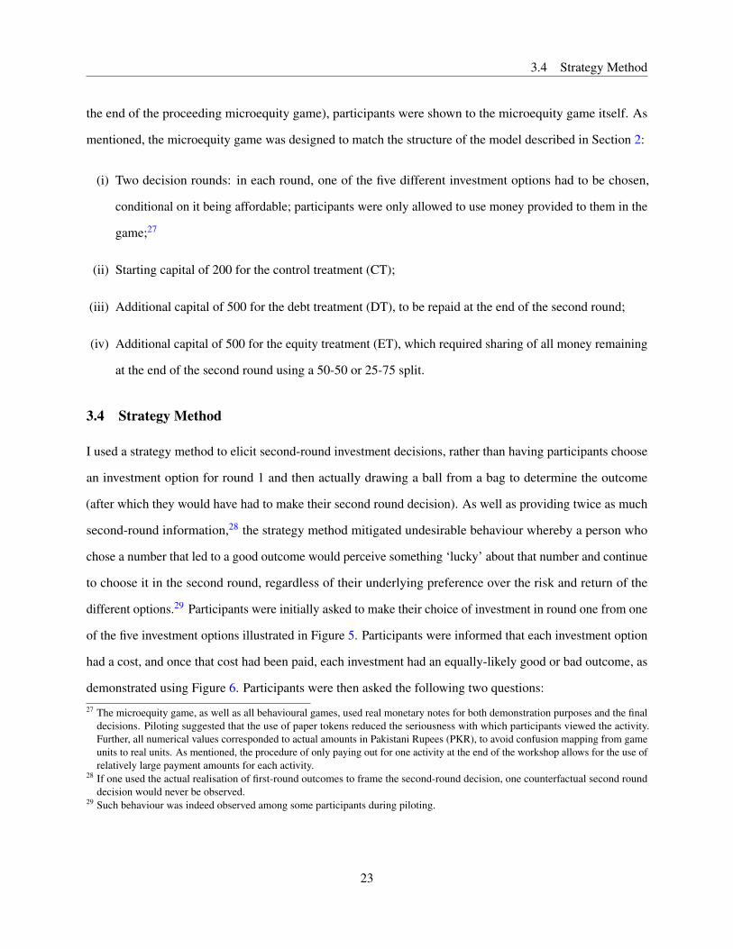
(i) Two decision rounds: in each round, one of the five different investment options had to be chosen,
conditional on it being affordable; participants were only allowed to use money provided to them in the
game;27
(ii) Starting capital of 200 for the control treatment (CT);
(iii) Additional capital of 500 for the debt treatment (DT), to be repaid at the end of the second round;
(iv) Additional capital of 500 for the equity treatment (ET), which required sharing of all money remaining
at the end of the second round using a 50-50 or 25-75 split.
3.4 Strategy Method
I used a strategy method to elicit second-round investment decisions, rather than having participants choose
an investment option for round 1 and then actually drawing a ball from a bag to determine the outcome
(after which they would have had to make their second round decision). As well as providing twice as much
second-round information,28 the strategy method mitigated undesirable behaviour whereby a person who
chose a number that led to a good outcome would perceive something ‘lucky’ about that number and continue
to choose it in the second round, regardless of their underlying preference over the risk and return of the
different options.29 Participants were initially asked to make their choice of investment in round one from one
of the five investment options illustrated in Figure 5. Participants were informed that each investment option
had a cost, and once that cost had been paid, each investment had an equally-likely good or bad outcome, as
demonstrated using Figure 6. Participants were then asked the following two questions:27 The microequity game, as well as all behavioural games, used real monetary notes for both demonstration purposes and the final
decisions. Piloting suggested that the use of paper tokens reduced the seriousness with which participants viewed the activity.Further, all numerical values corresponded to actual amounts in Pakistani Rupees (PKR), to avoid confusion mapping from gameunits to real units. As mentioned, the procedure of only paying out for one activity at the end of the workshop allows for the use ofrelatively large payment amounts for each activity.
28 If one used the actual realisation of first-round outcomes to frame the second-round decision, one counterfactual second rounddecision would never be observed.
29 Such behaviour was indeed observed among some participants during piloting.
23

3.4 Strategy Method
(i) "If the bad outcome occurs from the investment choice you just chose for the first round, which investment
option would you then choose in the second round?"
(ii) "What about if the good outcome occurs from the investment choice you just chose for the first round;
which investment option would you then choose in the second round?"
Figure 5: Set of investment options
Figure 6: Outcome of an investment option
Enumerators spent a considerable amount of time explaining the structure of the game to participants, and a
number of practice rounds were conducted to test understanding before the final decisions. Figure 7 illustrates
the tree diagram that was used to explain the structure of the entire game to participants.
24

3.5 Randomisation of Financial Contract Treatments
Figure 7: Game structure
3.5 Randomisation of Financial Contract Treatments
After completing a demonstration round with participants, where they practised the game under each treatment,
the final activity was conducted. To mitigate learning effects, the order in which the participants played the
three financial contract treatments was randomised.30 It is important to note that, when communicating with
participants, the word ‘treatment’ was never used, nor were the words ‘debt’ or ‘equity’; instead the more
neutral words ‘loan contract’ and ‘sharing contract’ were used (in the local language). The purpose of the
experiment was to study the effect of the contractual structure on investment behaviour, rather than any effect
driven by using those possibly emotive terms. However, all participants had previously taken a loan from
Akhuwat and successfully repaid it, and therefore it is much less likely that they would have had an aversion
to debt contracts.
4 Experimental results
In this section, I present results from the artefactual field experiment, which took place between December
2016 and February 2018. The main outcome variable, empirical specifications, and variables for heterogeneity30 In order to reduce confusion from switching from equity to debt and then back to equity, the two equity treatments always appeared
next to each other, although the order in which the two equity treatments appeared was also randomised.
25

4.1 Main result: Greater risk-taking under equity contract
analysis were pre-specified at the American Economic Association’s RCT Registry.31 The sample consists of
2,872 observations from 718 unique microenterprise owners, representing one decision per respondent for
each of the four treatment groups (CT, DT, ET1, ET2). Decisions under the two equity contracts are pooled
into one treatment indicator (ET) in the subsequent analysis.
4.1 Main result: Greater risk-taking under equity contract
Table 2 presents results using the following simple specification:
yi = β0 + β1DTi + β2ETi + εi (3)
where yi is the expected return of the investment options chosen by individual i in round 1, DTi is an indicator
variable that equals one for all investment decisions made under the debt treatment, and ETi is the equivalent
indicator variable for the equity treatments. Standard errors are clustered at the individual level. β0 represents
the average expected return of the investment option chosen by individuals in the control group, whilst β1 and
β2 represent the additional risk taken by debt-financed and equity-financed individuals relative to the control
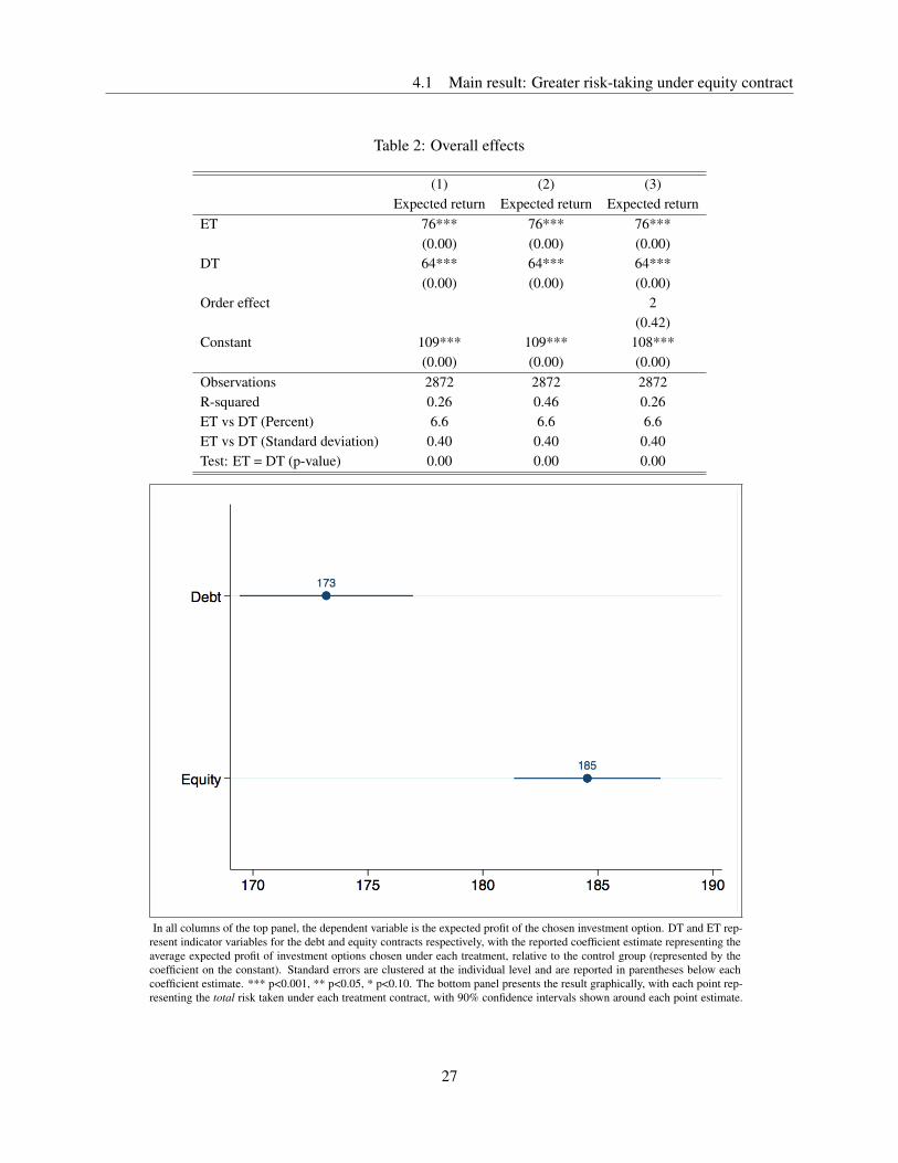
group, respectively. The main hypothesis I test is H0 : β1 = β2. Table 2 presents the main result of the
experiment. Equity-financed microenterprise owners chose investment options with an expected return of 185,
compared to an expected return of 173 under the debt contract. This represents an effect size of 0.40 standard
deviations of the control group’s distribution of investment choices, where the average expected return was
109, and is statistically significant at the 1% level. In Section 4.4, I present evidence that this overall result is
robust to a number of alternative specifications, including using the outcomes of second-round decisions.
Further, in Tables 3 - 9, where heterogeneous treatment analysis using a set of pre-specified variables is
presented, the average expected return under equity is greater than under debt in every sub-group.32
31 See https://www.socialscienceregistry.org/trials/2224.32 While all variables used in the heterogeneity analysis were pre-specified, the fact that they were trichotomised was not specified.
In each of Tables 3 - 9, I provide results using both a median split and terciles for the heterogeneity variable.
26
4.1 Main result: Greater risk-taking under equity contract
Table 2: Overall effects
(1) (2) (3)Expected return Expected return Expected return
ET 76*** 76*** 76***(0.00) (0.00) (0.00)
DT 64*** 64*** 64***(0.00) (0.00) (0.00)
Order effect 2(0.42)
Constant 109*** 109*** 108***(0.00) (0.00) (0.00)
Observations 2872 2872 2872R-squared 0.26 0.46 0.26ET vs DT (Percent) 6.6 6.6 6.6ET vs DT (Standard deviation) 0.40 0.40 0.40Test: ET = DT (p-value) 0.00 0.00 0.00
In all columns of the top panel, the dependent variable is the expected profit of the chosen investment option. DT and ET rep-resent indicator variables for the debt and equity contracts respectively, with the reported coefficient estimate representing theaverage expected profit of investment options chosen under each treatment, relative to the control group (represented by thecoefficient on the constant). Standard errors are clustered at the individual level and are reported in parentheses below eachcoefficient estimate. *** p<0.001, ** p<0.05, * p<0.10. The bottom panel presents the result graphically, with each point rep-resenting the total risk taken under each treatment contract, with 90% confidence intervals shown around each point estimate.
27

4.2 Heterogeneous treatment effects: Risk-aversion and loss-aversion
4.2 Heterogeneous treatment effects: Risk-aversion and loss-aversion
The purpose of the first section of heterogeneity analysis, presented in Tables 3 - 5, is to investigate potential
mechanisms through which the structure of contracts may affect investment behaviour. In all columns of
panel (a), the dependent variable is the expected profit of the chosen investment option. Columns (1), (2)
and (3) present results for the bottom, middle, and top terciles of the respective heterogeneity variable, while
columns (4) and (5) present results from the sub-sample with below- and above-median values respectively.
DT and ET are indicator variables for the debt and equity contracts respectively, with the reported coefficient
estimate indicating the average expected profit of investment options chosen under each treatment, relative to
the control group (represented by the coefficient on the constant). In the bottom panel of each table, results
are presented graphically, with each point illustrating the total risk taken under each treatment contract, with
90% confidence intervals shown around each point estimate.
4.2.1 Risk-aversion
Entrepreneurs who are more risk-averse may take relatively greater risk when financed with an equity contract,
where there is an insurance-like element through the explicit sharing of losses, compared to when they are
financed with a fixed-repayment debt contract. Tables 3 and 4 display regressions and graphical analysis
using the two different measures of risk-aversion. Each of the first three columns in the top panel shows a
separate regression using the specification in equation 3 for individuals in the different sub-groups.
Column (1) of Table 3 presents results for the least risk-averse entrepreneurs (the most ‘risk-tolerant’), with
column (2) showing results for those with an intermediate level of risk-aversion, and column (3) for the most
risk-averse, using the survey-based measure. In all three specifications, the expected return of investment
options chosen under equity is greater than that under debt, mirroring the overall results described in Section
4.1. The magnitude of the difference between risk-taking under equity compared to debt increases for the
most risk-averse microenterprise owners. Specifically, for the most risk-averse tercile, risk taken under equity
is 0.80 standard deviations greater than risk taken under debt, with the effect statistically significant at the
1% level. This compares to a difference of 0.29 and 0.15 standard deviations for the first two terciles of
risk-aversion respectively, using this survey-based measure. A similar result can be seen in the median split
28

4.2 Heterogeneous treatment effects: Risk-aversion and loss-aversion
Table 3: Heterogeneity analysis: Risk preferences (survey-based measure)
(1) (2) (3) (4) (5)Tercile 1 Tercile 2 Tercile 3 Below-median Above-median
ET 74*** 68*** 87*** 70*** 82***(0.00) (0.00) (0.00) (0.00) (0.00)
DT 66*** 64*** 64*** 62*** 67***(0.00) (0.00) (0.00) (0.00) (0.00)
Constant 113*** 110*** 103*** 113*** 105***(0.00) (0.00) (0.00) (0.00) (0.00)
Observations 928 1052 892 1500 1372R-squared 0.26 0.25 0.29 0.24 0.29ET vs DT (Percent) 4.6 2.5 13.7 4.8 8.5ET vs DT (Standard deviation) 0.29 0.15 0.80 0.29 0.51Test: ET = DT (p-value) 0.01 0.12 0.00 0.00 0.00
In all columns of the top panel, the dependent variable is the expected profit of the chosen investment option. Columns (1),(2) and (3) present results for the bottom, middle, and top terciles of the heterogeneity variable respectively. Columns (4) and(5) present results from the sub-sample with below- and above-median values respectively. ET and DT represent indicator vari-ables for the equity and debt contracts respectively, with the reported coefficient estimate representing the average expectedprofit of investment options chosen under each treatment, relative to the control group (represented by the coefficient on theconstant). Standard errors are clustered at the individual level and are reported in parentheses below each coefficient estimate.*** p<0.001, ** p<0.05, * p<0.10. Panel (b) presents the results from the heterogeneity analysis graphically, with each pointindicating the total risk taken under each treatment contract, with 90% confidence intervals shown around each point estimate.
29

4.2 Heterogeneous treatment effects: Risk-aversion and loss-aversion
analysis of columns (4) and (5), with an effect size of 0.29 standard deviations for those with below-median
risk-aversion and 0.51 standard deviations for those with above-median risk-aversion (both statistically
significant at the 1% level).
Turning to the incentivised measure of risk-aversion, Table 4 reveals that the most risk-tolerant tercile took on
average 0.36 standard deviations more risk under equity compared to debt, and that this magnitude increases
for those with intermediate risk-aversion, with an effect size of 0.48 standard deviations. For those who were
most risk-averse in the incentivised risk-aversion activity, the effect size decreases back down to 0.33 standard
deviations. The median-split analysis of columns (4) and (5) reveals an effect size of 0.36 standard deviations
for those with below-median risk-aversion and 0.43 standard deviations for those with above-median risk-
aversion (both statistically significant at the 1% level). One possible reason that the largest effect size is seen
with the top tercile of risk-aversion for the survey-based measure, whereas for the incentivised measure it was
seen with those with an intermediate level of risk-aversion, is that those who are defined as ‘most risk-averse’
using the incentivised measure are displaying quite an ‘extreme’ form of risk-aversion, compared to those
who are self-reporting as risk-averse in the survey-based measure. The two measures of risk-aversion are
significantly correlated, but the correlation coefficient is 0.267 for the raw measure and only 0.222 for the
trichotomised measure (both statistically significant at the 1% level), and thus the ‘most risk-averse’ group
defined by the two different measures could be quite distinct. Investigating the choices made by those in
the top tercile of the incentivised measures confirms the rather extreme level of risk-aversion; the average
person in the top tercile of risk-aversion rejected all 30 offers of the risky investment option, even when the
certain payment offered was only PKR 100 (compared to an average expected return of the risky investment
option of PKR 500, and even when the expected return of the risky option was increased to PKR 750). As a
comparison, the most risk-tolerant tercile on average only rejected 11 of the risky investment options, and
accepted 19 of them. It could be argued that this result for the most risk-averse tercile may be due to a cultural
‘gambling aversion’, given the Pakistani conservative Muslim context, yet all these participants who displayed
extreme risk-aversion were willing to make risky decisions in the microequity game. There were also no
reports of any of the microenterprise owners refusing to participate, so it appears that this behaviour does in
fact reflect an extreme form of risk-aversion. Referring back to the model predictions in Section 2, the effect
30

4.2 Heterogeneous treatment effects: Risk-aversion and loss-aversion
Table 4: Heterogeneity analysis: Risk preferences (incentivised measure)
(1) (2) (3) (4) (5)Tercile 1 Tercile 2 Tercile 3 Below-median Above-median
ET 71*** 79*** 77*** 69*** 82***(0.00) (0.00) (0.00) (0.00) (0.00)
DT 60*** 65*** 67*** 59*** 70***(0.00) (0.00) (0.00) (0.00) (0.00)
Constant 114*** 110*** 103*** 114*** 104***(0.00) (0.00) (0.00) (0.00) (0.00)
Observations 832 1056 984 1396 1476R-squared 0.23 0.30 0.26 0.24 0.29ET vs DT (Percent) 5.9 7.9 5.6 5.9 7.1ET vs DT (Standard deviation) 0.36 0.48 0.33 0.36 0.43Test: ET = DT (p-value) 0.00 0.00 0.00 0.00 0.00
In all columns of the top panel, the dependent variable is the expected profit of the chosen investment option. Columns (1),(2) and (3) present results for the bottom, middle, and top terciles of the heterogeneity variable respectively. Columns (4) and(5) present results from the sub-sample with below- and above-median values respectively. ET and DT represent indicator vari-ables for the equity and debt contracts respectively, with the reported coefficient estimate representing the average expectedprofit of investment options chosen under each treatment, relative to the control group (represented by the coefficient on theconstant). Standard errors are clustered at the individual level and are reported in parentheses below each coefficient estimate.*** p<0.001, ** p<0.05, * p<0.10. Panel (b) presents the results from the heterogeneity analysis graphically, with each pointindicating the total risk taken under each treatment contract, with 90% confidence intervals shown around each point estimate.
31

4.2 Heterogeneous treatment effects: Risk-aversion and loss-aversion
of equity contracts on risk-taking was expected to be most significant for those with greater risk-aversion,
while tailing off for those who were most risk-averse, and results in this section are consistent with that
prediction.
4.2.2 Loss-aversion
Entrepreneurs who are more loss-averse may take relatively less risk when financed by the debt contract,
compared to the equity contract, because of the prospect of defaulting on their debt contract and having money
deducted from the fixed participation fee that they are guaranteed for attending the workshop. Loss-averse
agents may be more willing to choose a higher expected return but riskier investment option when provided
with the implicit insurance of the equity contract, which mitigates the risk that they would lose some of their
own wealth, compared to the unlimited-liability debt contract.
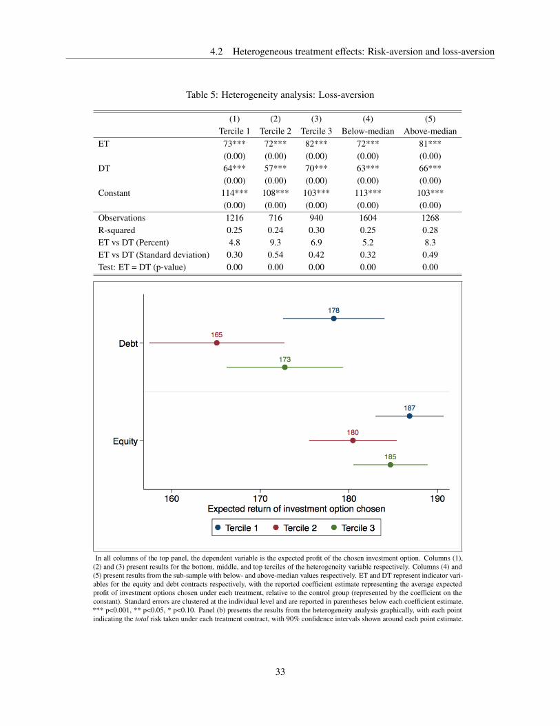
Table 5 presents regression and graphical analysis of results using the incentivised measure of loss-aversion.
Column (1) presents results for the least loss-averse entrepreneurs, with column (2) containing results for
those with an intermediate level of loss-aversion, and column (3) for the most loss-averse. In all specifications,
the expected return of investment options chosen under equity is greater than that under debt. As can be seen
graphically, the magnitude of the difference between risk-taking under equity compared to debt increases for
those with an intermediate level of loss-aversion, compared to those who are the least lost averse. Specifically,
for the least loss-averse group, risk taken under equity is 0.30 standard deviations greater than risk taken
under debt, with the difference statistically significant at the 1% level. For those with an intermediate level
of loss-aversion, risk taken under equity is 0.54 standard deviations greater than risk taken under debt, and
significant at the 1% level. Finally, for the most loss-averse group, the effect size is smaller, at 0.42 standard
deviations, significant at the 1% level, and mirroring the results for the incentivised risk-aversion measure in
Table 4. The median split analysis of columns (4) and (5) reveals an effect size of 0.32 standard deviations
for those with below-median loss-aversion and 0.49 standard deviations for those with above-median loss-
aversion.
32
4.2 Heterogeneous treatment effects: Risk-aversion and loss-aversion
Table 5: Heterogeneity analysis: Loss-aversion
(1) (2) (3) (4) (5)Tercile 1 Tercile 2 Tercile 3 Below-median Above-median
ET 73*** 72*** 82*** 72*** 81***(0.00) (0.00) (0.00) (0.00) (0.00)
DT 64*** 57*** 70*** 63*** 66***(0.00) (0.00) (0.00) (0.00) (0.00)
Constant 114*** 108*** 103*** 113*** 103***(0.00) (0.00) (0.00) (0.00) (0.00)
Observations 1216 716 940 1604 1268R-squared 0.25 0.24 0.30 0.25 0.28ET vs DT (Percent) 4.8 9.3 6.9 5.2 8.3ET vs DT (Standard deviation) 0.30 0.54 0.42 0.32 0.49Test: ET = DT (p-value) 0.00 0.00 0.00 0.00 0.00
In all columns of the top panel, the dependent variable is the expected profit of the chosen investment option. Columns (1),(2) and (3) present results for the bottom, middle, and top terciles of the heterogeneity variable respectively. Columns (4) and(5) present results from the sub-sample with below- and above-median values respectively. ET and DT represent indicator vari-ables for the equity and debt contracts respectively, with the reported coefficient estimate representing the average expectedprofit of investment options chosen under each treatment, relative to the control group (represented by the coefficient on theconstant). Standard errors are clustered at the individual level and are reported in parentheses below each coefficient estimate.*** p<0.001, ** p<0.05, * p<0.10. Panel (b) presents the results from the heterogeneity analysis graphically, with each pointindicating the total risk taken under each treatment contract, with 90% confidence intervals shown around each point estimate.
33

4.3 Heterogeneous effects: Management practices and education
Analysing the behaviour of the most loss-averse microenterprise owners (the top tercile of loss-aversion)
sheds light on why the effect is smaller relative to those with an intermediate amount of loss-aversion, as was
clear in the analysis of the most risk-averse tercile in the incentivised risk measure. Individuals in the most
loss-averse tercile made an average of 9 rejection decisions, meaning that they rejected investment options that
involved either winning PKR 1,000 with probability 0.5 or losing PKR 200 with probability 0.5 (an expected
value of 400), and 8 other similar investment options that led to winning PKR 1,000 or losing amounts greater
than PKR 200 (in increments of PKR 100). As a comparison, the least loss-averse individuals only rejected 4
of the 10 investment options. Therefore, those in the most loss-averse tercile could be considered to have
quite an ‘extreme’ amount of loss-aversion, as was the case with those in the top tercile of the incentivised
risk-aversion activity; in fact, the correlation between responses in the incentivised loss-aversion activity and
the incentivised risk preference elicitation activity is actually higher than that between the two risk preference
activities (a correlation of 0.302 in the raw data, and 0.319 for the trichotomised measure, both statistically
significant at the 1% level).
4.3 Heterogeneous effects: Management practices and education
The purpose of the first section of heterogeneity analysis was to explore heterogeneous treatment effects by
variables that illustrate potential mechanisms through which the structure of contracts may affect investment
behaviour. Results in Section 4.2 reveal that more risk-averse and more loss-averse individuals chose
investment options with a greater expected return under equity financing than under debt financing. While
there could be positive welfare effects in stimulating profitable investments for individuals whose behavioural
characteristics lead them to relatively under-invest, from a policy perspective MFIs may not wish to provide
such financing if those individuals have the worst business management practices, and the lowest education
and cognitive ability. In this section I conduct a similar heterogeneity analysis for those variables, and
confirm that such a concern is unfounded; there is no evidence that the microenterprise owners with the
lowest business management practices, education or cognitive ability are those for whom equity contracts are
incentivising the greatest risk-taking relative to debt; in fact, there is some evidence of the opposite effect.
34

4.3 Heterogeneous effects: Management practices and education
4.3.1 Management practices
From a policy perspective, it is important to understand what the treatment effect is for microenterprise
owners with better management practices, for example record-keeping and a clear separation of business and
household finances. Equity financing, which requires accurate reporting of performance for the purposes of
profit- and loss- sharing, is less viable for individuals who do not keep records of their assets, incomes and
expenses, or who frequently combine business and household accounts. If individuals with better management
practices take more risk under equity financing, this provides promising evidence for the potential impact of an
equity-based product in the field. A recent literature has highlighted the importance of business management
practices for performance of firms in developed countries (Bloom and Van Reenen, 2010). McKenzie and
Woodruff (2016) develop a set of questions that have been adapted for microenterprises in a developing
country setting, which I used to measure business management practices for the participants in my sample.
The questions covered the following areas:
(i) Marketing (whether the firm advertises, attempts to attract customers with a special offer, and if it
solicits customer feedback on what other products they would like it to sell);
(ii) Record-keeping (whether the firm records its sales and purchases, if it has calculated the cost and profit
margin of its main products, and whether it has a written budget);
(iii) Financial planning (whether the firm has a sales target, and if it keeps a balance sheet and profit and
loss statement);
(iv) Buying and stock control (whether it frequently runs out of stock, and if it attempts to negotiate with
suppliers).
I aggregated all positive responses into a business management practices index. Results in Table 6 reveal
that, as with all previous specifications, average risk-taking is greater under equity than debt for each sub-
group. It can also be observed that the size of the effect is increasing for those with higher management
practices; those in the lowest tercile of management practices take 0.29 standard deviations greater risk
under equity (significant at the 5% level), with an effect size of 0.43 standard deviations for those with
intermediate management practices and 0.45 standard deviations for the highest management practices group
(both significant at the 1% level). A similar result is reflected in the median-split analysis (0.33 and 0.46
35

4.3 Heterogeneous effects: Management practices and education
Table 6: Heterogeneity analysis: Business management practices
(1) (2) (3) (4) (5)Tercile 1 Tercile 2 Tercile 3 Below-median Above-median
ET 62*** 79*** 84*** 70*** 81***(0.00) (0.00) (0.00) (0.00) (0.00)
DT 54*** 66*** 71*** 61*** 68***(0.00) (0.00) (0.00) (0.00) (0.00)
Constant 111*** 108*** 108*** 110*** 108***(0.00) (0.00) (0.00) (0.00) (0.00)
Observations 840 1044 988 1412 1460R-squared 0.21 0.29 0.29 0.25 0.28ET vs DT (Percent) 5.1 7.0 7.2 5.6 7.5ET vs DT (Standard deviation) 0.29 0.43 0.45 0.33 0.46Test: ET = DT (p-value) 0.01 0.00 0.00 0.00 0.00
In all columns of the top panel, the dependent variable is the expected profit of the chosen investment option. Columns (1),(2) and (3) present results for the bottom, middle, and top terciles of the heterogeneity variable respectively. Columns (4) and(5) present results from the sub-sample with below- and above-median values respectively. ET and DT represent indicator vari-ables for the equity and debt contracts respectively, with the reported coefficient estimate representing the average expectedprofit of investment options chosen under each treatment, relative to the control group (represented by the coefficient on theconstant). Standard errors are clustered at the individual level and are reported in parentheses below each coefficient estimate.*** p<0.001, ** p<0.05, * p<0.10. Panel (b) presents the results from the heterogeneity analysis graphically, with each pointindicating the total risk taken under each treatment contract, with 90% confidence intervals shown around each point estimate.
36

4.3 Heterogeneous effects: Management practices and education
standard deviation effect sizes for those with below-median and above-median management practices
respectively, with both effects significant at the 1% level). Overall, results are promising because they indicate
that equity contracts had the greatest impact on risk-taking for those microenterprise owners with the best
management practices.
4.3.2 Education and cognitive ability
Equity contracts may be relatively unfamiliar to many participants and need more cognitive processing than
simple fixed-repayment debt contracts, since they require individuals to calculate income-sharing payments
of 25%, 50% and 75%. Individuals with lower cognitive ability may struggle with such calculations. While
the education variable was simply measured as the highest completed level of formal education, cognitive
ability was measured using a set of number recall activities and addition, subtraction and division questions,
with scores aggregated into an index.
Tables 7 and 8 provide evidence that the largest effect of equity financing was amongst those with the highest
education and cognitive ability respectively. Individuals in the lowest tercile of education took 0.28 standard
deviations greater risk under equity, with an effect size of 0.48 and 0.43 standard deviations for those with
intermediate and the highest levels of education respectively. Similar evidence is provided using scores from
a mathematical test that was administered with all participants during the workshop, with an effect size of
0.30 standard deviations for the lowest tercile of maths score, and 0.45 and 0.42 standard deviations for those
with intermediate and the highest maths scores respectively, with the effects statistically significant in all
specifications.
Overall, results from this section of heterogeneity analysis provide encouraging evidence from a policy
perspective that the greatest effect of equity contracts was on those microenterprise owners who had the
highest education, cognitive ability and management practices. These individuals are those to whom MFIs
may be most willing to offer equity-based products, since such contracts involve keeping records, separating
household and business accounts, and making non-standard calculations for profit shares.
37

4.3 Heterogeneous effects: Management practices and education
Table 7: Heterogeneity analysis: Years of education
(1) (2) (3) (4) (5)Tercile 1 Tercile 2 Tercile 3 Below-median Above-median
ET 72*** 80*** 76*** 76*** 76***(0.00) (0.00) (0.00) (0.00) (0.00)
DT 64*** 66*** 63*** 65*** 63***(0.00) (0.00) (0.00) (0.00) (0.00)
Constant 109*** 108*** 109*** 109*** 109***(0.00) (0.00) (0.00) (0.00) (0.00)
Observations 972 836 1064 1628 1244R-squared 0.24 0.30 0.26 0.27 0.26ET vs DT (Percent) 4.6 8.0 7.2 6.0 7.3ET vs DT (Standard deviation) 0.28 0.48 0.43 0.36 0.44Test: ET = DT (p-value) 0.02 0.00 0.00 0.00 0.00
In all columns of the top panel, the dependent variable is the expected profit of the chosen investment option. Columns (1),(2) and (3) present results for the bottom, middle, and top terciles of the heterogeneity variable respectively. Columns (4) and(5) present results from the sub-sample with below- and above-median values respectively. ET and DT represent indicator vari-ables for the equity and debt contracts respectively, with the reported coefficient estimate representing the average expectedprofit of investment options chosen under each treatment, relative to the control group (represented by the coefficient on theconstant). Standard errors are clustered at the individual level and are reported in parentheses below each coefficient estimate.*** p<0.001, ** p<0.05, * p<0.10. Panel (b) presents the results from the heterogeneity analysis graphically, with each pointindicating the total risk taken under each treatment contract, with 90% confidence intervals shown around each point estimate.
38
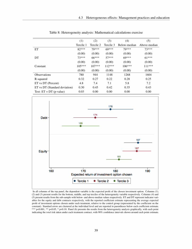
4.3 Heterogeneous effects: Management practices and education
Table 8: Heterogeneity analysis: Mathematical calculations exercise
(1) (2) (3) (4) (5)Tercile 1 Tercile 2 Tercile 3 Below-median Above-median
ET 82*** 79*** 69*** 79*** 73***(0.00) (0.00) (0.00) (0.00) (0.00)
DT 73*** 66*** 57*** 69*** 61***(0.00) (0.00) (0.00) (0.00) (0.00)
Constant 105*** 107*** 112*** 106*** 111***(0.00) (0.00) (0.00) (0.00) (0.00)
Observations 780 944 1148 1268 1604R-squared 0.32 0.27 0.22 0.28 0.25ET vs DT (Percent) 4.8 7.4 7.1 5.8 7.2ET vs DT (Standard deviation) 0.30 0.45 0.42 0.35 0.43Test: ET = DT (p-value) 0.03 0.00 0.00 0.00 0.00
In all columns of the top panel, the dependent variable is the expected profit of the chosen investment option. Columns (1),(2) and (3) present results for the bottom, middle, and top terciles of the heterogeneity variable respectively. Columns (4) and(5) present results from the sub-sample with below- and above-median values respectively. ET and DT represent indicator vari-ables for the equity and debt contracts respectively, with the reported coefficient estimate representing the average expectedprofit of investment options chosen under each treatment, relative to the control group (represented by the coefficient on theconstant). Standard errors are clustered at the individual level and are reported in parentheses below each coefficient estimate.*** p<0.001, ** p<0.05, * p<0.10. Panel (b) presents the results from the heterogeneity analysis graphically, with each pointindicating the total risk taken under each treatment contract, with 90% confidence intervals shown around each point estimate.
39

4.4 Robustness checks
4.3.3 Trust
The final pre-specified variable for heterogeneity analysis is trust. Trust is potentially quite important in
the comparison between equity contracts, which involve sharing of profits and losses, and fixed-repayment
debt contracts. Since individuals who are less trusting may be less inclined to choose equity financing in the
field, understanding the treatment effect for more trusting individuals is important from a policy perspective.
Trust was measured using a series of questions from the General Social Survey (GSS).33 Table 9, as with
all previous tables, shows greater risk-taking under equity compared to debt, for all terciles. The magnitude
of the effect is 0.21 standard deviations for the least trusting, 0.40 standard deviations for those with an
intermediate level of trust, and 0.52 standard deviations for the most trusting.
4.4 Robustness checks
As seen in Table 2 and the subsequent heterogeneity analysis of Tables 3 - 9, risk-taking under equity was
greater than that under debt, with the effect evident in every sub-group used in the heterogeneity analysis.
While this provides strong evidence for the effects, in this section I present further robustness checks by
investigating second-round decisions and order effects.
4.4.1 Second-round decisions
Table 10 illustrates results for the investment options chosen in the second decision round, using the strategy
method described in Section 3.4. In columns (1) and (2) the analysis is done for second-round decisions
conditional on a bad outcome occurring in the first round, and in columns (3) and (4) the analysis is done
conditional on a good outcome having occurred in the first round. Columns (1) and (3) present results from
specifications with simple treatment dummies and a dummy for basic order effects, while columns (2) and (4)
include dummies that fully control for the endogeneity that is inherent in columns (1) and (3). Decisions in
the second round are endogenous to the previous investment decision made by participants, which in this
setting can be fully controlled for by including dummies for the decision made in the first round.
33 As used by Giné, Jakiela, Karlan, and Morduch (2010).
40

4.4 Robustness checks
Table 9: Heterogeneity analysis: Trust
(1) (2) (3) (4) (5)Tercile 1 Tercile 2 Tercile 3 Below-median Above-median
ET 75*** 75*** 78*** 75*** 76***(0.00) (0.00) (0.00) (0.00) (0.00)
DT 68*** 63*** 63*** 67*** 62***(0.00) (0.00) (0.00) (0.00) (0.00)
Constant 109*** 108*** 110*** 106*** 111***(0.00) (0.00) (0.00) (0.00) (0.00)
Observations 640 1344 888 1336 1536R-squared 0.26 0.26 0.28 0.27 0.26ET vs DT (Percent) 3.4 6.7 8.6 4.9 8.0ET vs DT (Standard deviation) 0.21 0.40 0.52 0.30 0.48Test: ET = DT (p-value) 0.11 0.00 0.00 0.00 0.00
In all columns of the top panel, the dependent variable is the expected profit of the chosen investment option. Columns (1),(2) and (3) present results for the bottom, middle, and top terciles of the heterogeneity variable respectively. Columns (4) and(5) present results from the sub-sample with below- and above-median values respectively. ET and DT represent indicator vari-ables for the equity and debt contracts respectively, with the reported coefficient estimate representing the average expectedprofit of investment options chosen under each treatment, relative to the control group (represented by the coefficient on theconstant). Standard errors are clustered at the individual level and are reported in parentheses below each coefficient estimate.*** p<0.001, ** p<0.05, * p<0.10. Panel (b) presents the results from the heterogeneity analysis graphically, with each pointindicating the total risk taken under each treatment contract, with 90% confidence intervals shown around each point estimate.
41

4.4 Robustness checks
Column (1) reveals that in the second round, conditional on a bad outcome occurring in the first round,
risk-taking under equity was 0.40 standard deviations greater than risk-taking under debt, with the difference
statistically significant at the 1% level. Inclusion of dummies for endogenous selection does not significantly
change the outcome; column (2) shows that equity-financed microenterprise owners took 0.29 standard devia-
tions greater risk than those who were debt-financed, with the effect still statistically significant at the 1% level.
Table 10: Second-round decisions.
(1) (2) (3) (4)R2|R1bad R2|R1bad R2|R1good R2|R1good
Constant 77*** 44*** 176*** 110***(0.00) (0.00) (0.00) (0.00)
DT 65*** 52*** 24*** -14***(0.00) (0.00) (0.00) (0.00)
ET 75*** 59*** 32*** -13***(0.00) (0.00) (0.00) (0.00)
Order 0 0 1 -1(0.87) (1.00) (0.84) (0.72)
R1:Inv2 37*** 65***(0.00) (0.00)
R1:Inv3 37*** 94***(0.00) (0.00)
R1:Inv4 64*** 125***(0.00) (0.00)
R1:Inv5 60*** 148***(0.00) (0.00)
Observations 2872 2872 2872 2872R-squared 0.34 0.41 0.05 0.37ET vs DT (Percent) 7.2 7.7 3.9 0.6ET vs DT (Standard deviation) 0.40 0.29 0.14 0.01Test: ET = DT (p-value) 0.00 0.00 0.00 0.71
While column (3) also reveals greater risk-taking under equity in the second decision round conditional on a
good outcome occurring in the first round, with an effect size of 0.14 standard deviations (significant at the
1% level), inclusion of dummies for first-round decisions leads to this effect almost completely disappearing
(to 0.01 standard deviations, statistically indistinguishable from zero). In fact, inclusion of the first-round
dummies reveals that the coefficients on the debt and equity treatments are actually negative and of similar
magnitude, implying less risk-taking relative to the control group. This could indicate an income effect,
whereby entrepreneurs who were externally financed, by either debt or equity, are implicitly being taxed
42

4.4 Robustness checks
on their gains, with some portion being returned either as a loan repayment or an equity sharing amount,
whereas the control group accrue the full additional benefits of the positive investment outcomes.
4.4.2 Order effects
As described in Section 3, the experiment used a within-subject design, where each microenterprise owner
made investment decisions under all treatments, with the order of the financing treatments randomised.
Column (1) of Table 11 presents regression analysis with the same simple controls for order effects as in
previous regressions, as well as the addition of interaction terms between the order and treatments, where
‘Order’ is an indicator variable for whether debt (randomly) appeared as the first treatment. Column (2)
illustrates the analysis for only those observations where debt was randomly revealed first, and column (3)
displays results when equity appeared first. Risk-taking under equity is significantly greater than risk-taking
under debt, regardless of whether debt or equity appear first, although there is some difference in magnitude.
Column (3) reveals that when equity appeared first, risk-taking under equity was greater by 0.53 standard
deviations, significant at the 1% level. The effect decreases to 0.25 standard deviations greater risk-taking
under equity when debt appears first, but is still highly significant (p-value 0.010). As can be seen in columns
(2) and (3), risk-taking under equity is at approximately the same level regardless of whether debt or equity
appear first in the order, however risk-taking under debt is lower when it appears after equity. One possible
interpretation is that, having experienced the risk-sharing contract, individuals are subsequently less likely
to take risk under debt as they have learned about the insurance-like benefits of the equity contract, which
are absent from a fixed-repayment loan contract. Nonetheless, as mentioned, risk-taking under equity is still
significantly greater than risk-taking under debt, even when debt appears first.
43

4.4 Robustness checks
Table 11: Order effects.
(1) (2) (3)ExpRet ExpRet ExpRet
Constant 109*** 108*** 109***(0.00) (0.00) (0.00)
DT 59*** 70*** 59***(0.00) (0.00) (0.00)
ET 75*** 77*** 75***(0.00) (0.00) (0.00)
Order -1(0.61)
DT:Ord1 10**(0.03)
ET:Ord1 2(0.62)
Observations 2872 1412 1460R-squared 0.27 0.28 0.25ET vs DT (Percent) 4.1 9.1ET vs DT (Standard deviation) 0.25 0.53Test: ET = DT (p-value) 0.01 0.00
4.4.3 LASSO
In this section, I use a simple machine learning technique as a robustness check for the heterogeneity analysis
of Sections 4.2 and 4.3. Specifically, the Least Absolute Shrinkage and Selection Operator (LASSO) and
Post-LASSO estimator proposed by Belloni, Chernozhukov, and Hansen (2014) is employed. The Post-
LASSO estimator (and other high-dimensional model selection methods) can be a useful forecasting tool
when there are a large number of potentially informative covariates. For a simple model:
yi =
p∑j=1
βjxij + ui
LASSO coefficients are chosen to minimise the sum of squared residuals plus a penalty term that penalises
the size of the model through the sum of absolute values of the coefficients:
β̂ = argminb
n∑i=1
(yi −
p∑j=1
xijbj
)2
+ λ
p∑j=1
|bj |γj
44

4.4 Robustness checks
where λ is a penalty parameter and γj are penalty loadings. One issue with this estimator is that non-zero
coefficients that are part of the solution to the LASSO problem tend to be biased towards zero. The Post-
LASSO estimator first applies LASSO to determine which variables can be dropped from the standpoint of
prediction, and then estimates coefficients on the remaining variables using ordinary least squares. Table 12
presents results from LASSO estimation. In the top panel, all variables that were used for the purposes of
heterogeneity analysis in Sections 4.2 and 4.3 are included in their trichotomised form. In the bottom panel, I
also add a number of other potentially important business and household characteristics: business revenues
and profits, business fixed assets and current assets, household income and expenditure, and household assets,
savings and loans. Column (1) presents results from the initial LASSO estimation, and column (2) displays
Post-LASSO coefficients.
Unsurprisingly, LASSO estimation identifies the two most important variables for predicting the outcome
variable of expected return of investment chosen as the debt and equity treatment indicator variables, DT
and ET. The top panel also identifies risk-aversion and loss-aversion as important variables for predicting
risk taking, independently of their interaction with the treatment variables. Both coefficients are negative,
indicating that more risk- and loss-averse microenterprise owners chose investment options with a lower
expected return and risk, on average. Results also confirm the findings of Section 4.2: more risk-averse
individuals chose investment options with a higher expected return when financed with the equity contract, as
indicated by the selection of the interaction between ET and the two different measures of risk-aversion in
the LASSO estimation (specifically, the third tercile of risk-aversion for the survey-based measure, and the
second tercile of risk-aversion for the incentivised measure). In contrast, LASSO dropped the interaction
between DT and risk-aversion measures. Further, in the top panel, the LASSO specification also selected the
interaction between ET and the top two terciles of management practices, as well as the top tercile of the
trust measure, with a positive coefficient indicating greatest risk-taking when individuals with the highest
management practices and the highest level of trust are equity-financed. The only debt-interacted variable
selected in the top panel is the interaction between DT and the top tercile of management practices.
45

4.4 Robustness checks
Table 12: LASSO
The top panel presents results from a LASSO and Post-LASSO estimation using all vari-ables that were used for heterogeneity analysis in Sections 4.2 and 4.3, in their tri-chotomised form. The dependent variable is the expected profit of the chosen investmentoption. In the bottom panel, a number of other potentially important variables are addedin their trichotomised form: business revenues and profits, business fixed assets and cur-rent assets, household income and expenditure, and household assets, savings and loans.
46

Implementing microequity contracts in the field
Results in the bottom panel, when including a number of other business and household characteristics, reveal
the robustness of the findings in the top panel; the LASSO estimator continues to select the interaction between
equity financing and risk-aversion, management practices and trust as important variables in predicting the
outcome variable. Further, a number of other variables that capture business size and household wealth are
also found to be important determinants of risk-taking when interacted with both treatment variables (with the
majority of the selected variables being those interacted with the equity financing indicator). As discussed by
Mullainathan and Spiess (2017), the purpose of LASSO and other machine learning algorithms is prediction
and not parameter estimation, so one should be cautious in providing too much interpretation to these results.
The purpose of this section was to provide an additional robustness check, which confirms the importance
of risk-aversion when interacted with equity financing. However, the fact that loss-aversion was dropped
by the LASSO estimator does not indicate that loss-aversion is not an important factor; it could simply be
that risk-aversion is more accurately measured than loss-aversion in the behavioural games activities, which
would not be surprising, given that there were many more questions dedicated to measuring risk preferences.
5 Implementing microequity contracts in the field
Results in Section 4 reveal that equity contracts led to greater risk-taking compared to debt-based contracts,
and that the effect was particularly strong for the more risk-averse and loss-averse entrepreneurs, who might
ordinarily under-invest. Further, the second part of the heterogeneity analysis provides evidence that mitigates
adverse-selection-type concerns that those microenterprise owners who are most encouraged to take more
risk with equity financing might be those with the worst business management practices, education and
cognitive ability, which has important implications for the viability of implementing equity contracts in the
field. Given the positive results, it is important to investigate why we do not typically observe MFIs imple-
menting microequity contracts in the field. The majority of microcredit contracts have a very rigid structure,
and – although there are recent researcher-led efforts to introduce more flexible microcredit contracts – to
my knowledge there is no organisation that is implementing performance-contingent-repayment contracts
with microenterprises on any meaningfully large scale. Theoretical work suggests that equity contracts are
non-optimal relative to debt due to costly state verification (Townsend, 1979) and moral hazard (Stiglitz and
Weiss, 1981), although those results only hold for a risk-neutral agent and a fixed-repayment contract may be
47

5.1 Summary statistics
sub-optimal for a risk-averse agent. Given many MFIs’ stated objectives to prioritise borrower welfare as well
as profits, it is peculiar that no large MFI is implementing microequity contracts, given the potential benefits
discussed in the artefactual field experiment in this paper, in particular for individuals whose behavioural
characteristics such as risk- and loss-aversion may lead them to under-invest. In this section, I provide some
evidence that sheds light on some of the most important constraints to implementing microequity contracts in
the field, using a survey that I designed to investigate a microequity program that had been initiated by one of
the largest microfinance institutions in Pakistan, the National Rural Support Programme (NRSP).34
NRSP is the largest rural support programme in Pakistan, with a presence in 64 districts across all four
provinces, and currently working with 3 million poor households. In September 2014, NRSP launched
a microequity program that aimed to help skilled apprentices start their own business by providing them
with equity-like capital. As of August 2015, 1,250 individuals had been provided with financing as part of
this program, in five major districts across Punjab and Islamabad.35 I generated a stratified random sample
from the population of 1,250 clients, based on the following variables: (i) gender; (ii) business type (trade,
manufacturing or services); (iii) district; and (iv) age of entrepreneur (using a median-split). This generated
60 distinct blocks, from which a random sample of 248 individuals was drawn.36
5.1 Summary statistics
Tables 13 and 14 present summary statistics. 90% of clients were male, with a mean age of 33. The average
years of education was eight, and 95% of clients could read Urdu. 73% of clients were married, and the
average household size was approximately seven. 96% of respondents were managing a business, with 88%
of them only running one business (79% owned that business themselves). On average, they had seven years
of experience in the sector to which their business related (either managing a business, or as an apprentice).
81% of businesses were initially set up by the respondent. 61% of businesses had no other employees, with
20% having one additional employee and 12% having two additional employees. Only 2% of respondents34 I learned about this program in the course of fieldwork for the artefactual field experiment; the program had started before my
activities with Akhuwat and I was invited by the CEO of NRSP to conduct a survey to evaluate the implementation of thesemicroequity contracts in the field.
35 In Attock, Chakwal, ICT, Jhelum, and Mandi Bahauddin.36 All surveys were then conducted by enumerators at the microenterprise’s location of business.
48
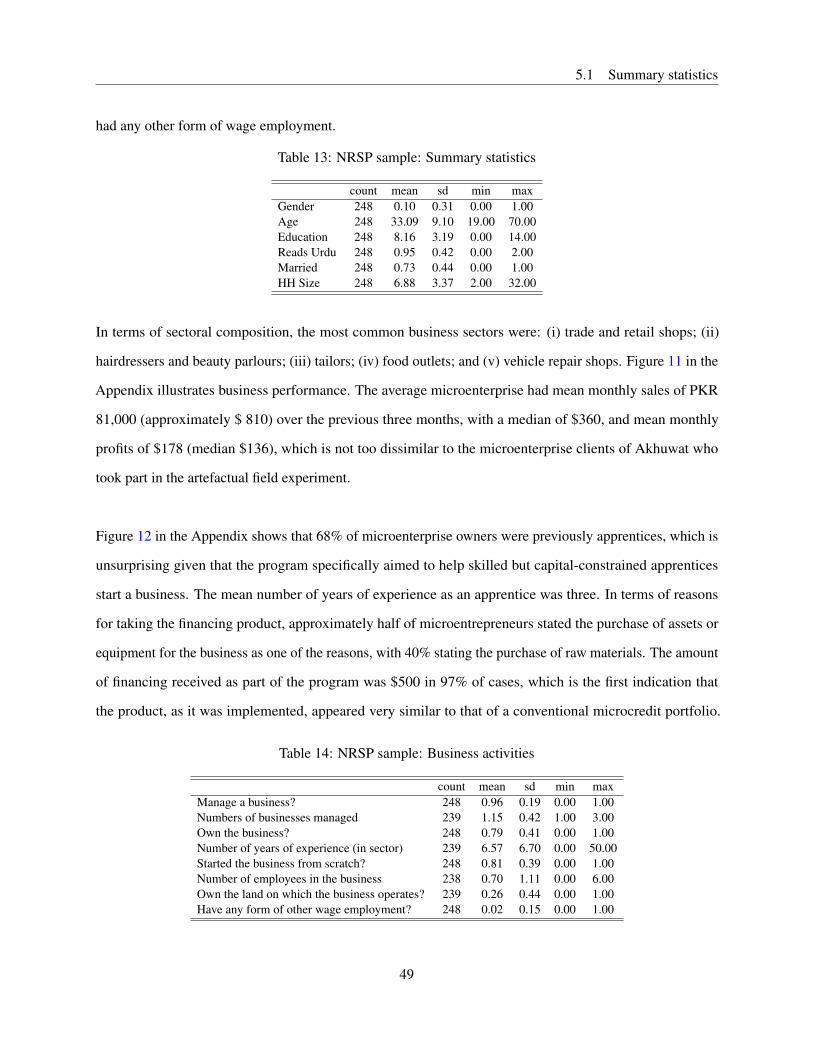
5.1 Summary statistics
had any other form of wage employment.
Table 13: NRSP sample: Summary statistics
count mean sd min maxGender 248 0.10 0.31 0.00 1.00Age 248 33.09 9.10 19.00 70.00Education 248 8.16 3.19 0.00 14.00Reads Urdu 248 0.95 0.42 0.00 2.00Married 248 0.73 0.44 0.00 1.00HH Size 248 6.88 3.37 2.00 32.00
In terms of sectoral composition, the most common business sectors were: (i) trade and retail shops; (ii)
hairdressers and beauty parlours; (iii) tailors; (iv) food outlets; and (v) vehicle repair shops. Figure 11 in the
Appendix illustrates business performance. The average microenterprise had mean monthly sales of PKR
81,000 (approximately $ 810) over the previous three months, with a median of $360, and mean monthly
profits of $178 (median $136), which is not too dissimilar to the microenterprise clients of Akhuwat who
took part in the artefactual field experiment.
Figure 12 in the Appendix shows that 68% of microenterprise owners were previously apprentices, which is
unsurprising given that the program specifically aimed to help skilled but capital-constrained apprentices
start a business. The mean number of years of experience as an apprentice was three. In terms of reasons
for taking the financing product, approximately half of microentrepreneurs stated the purchase of assets or
equipment for the business as one of the reasons, with 40% stating the purchase of raw materials. The amount
of financing received as part of the program was $500 in 97% of cases, which is the first indication that
the product, as it was implemented, appeared very similar to that of a conventional microcredit portfolio.
Table 14: NRSP sample: Business activities
count mean sd min maxManage a business? 248 0.96 0.19 0.00 1.00Numbers of businesses managed 239 1.15 0.42 1.00 3.00Own the business? 248 0.79 0.41 0.00 1.00Number of years of experience (in sector) 239 6.57 6.70 0.00 50.00Started the business from scratch? 248 0.81 0.39 0.00 1.00Number of employees in the business 238 0.70 1.11 0.00 6.00Own the land on which the business operates? 239 0.26 0.44 0.00 1.00Have any form of other wage employment? 248 0.02 0.15 0.00 1.00
49

5.2 NRSP contract structure
Given the heterogeneity in business sector and business performance observed in Figure 11, some variation
in financing amount might have been expected.
5.2 NRSP contract structure
The main purpose of the survey was to investigate the structure of the contracts that were intended to be
implemented as ‘microequity’, as described by clients who were provided with financing. Figures 8, 9 and 10
illustrate the results. It is clear that NRSP had started implementing the product as an equity-based contract,
for which there was a pre-agreed profit- and loss-sharing ratio of 20-80 (with the entrepreneur sharing 20% of
their monthly profits with NRSP, and keeping 80% for themselves). As observed in Figure 8, when asked what
the ‘profit-sharing ratio’ was between them and NRSP, 50% of respondents answered “80-20”, which reflects
the actual profit- and loss-sharing ratio with which the program started. Over 30% of respondents, however,
stated that they did not know the profit-sharing ratio; post-survey follow-up conversations with enumerators
suggested a lack of comprehension of this question. In hindsight, this reflects many entrepreneurs’ inability
to understand a question about sharing ratios when the way in which the product was being implemented at
the time of the survey very much resembled a conventional fixed-repayment debt product. The next graph
in Figure 8 again provides evidence that the way the contracts were being implemented in the field at the
time of the survey mirrored a conventional debt contract with one set of standard terms and conditions
implemented by all NRSP field staff. Here, it is clear that the repayment payment frequency was monthly
for all entrepreneurs. While this is not sufficient evidence in itself that the product being offered was not
equity-like, some variation in payment frequency might have been expected if a true equity-like product was
being implemented.
The next two questions were the most significant in the survey; if what was being implemented was truly an
equity-like product with performance-contingent payments, then one would expect some correlation between
microenterprise business outcomes and actual payments made to NRSP. The following questions were asked:
(i) "Think about the current contract that you have with NRSP. If you have zero profits in a given period
that you usually make payments, how much do you have to pay to NRSP?"
(ii) "Think about the current contract that you have with NRSP. If you have very big profits in a given period,
50

5.2 NRSP contract structure
how much do you have to pay to NRSP?"
Figure 8: Contract structure questions 1
The results, illustrated in the third and fourth graphs in Figure 8, are very clear; in 85% of cases, the respon-
dent stated that there was no profit- or loss-sharing involved in their relationship with NRSP: when their
business profits were low, their repayments stayed the same, and when their business profits were high, their
repayments again remained constant. This provides conclusive evidence that what was being implemented in
the field was not equity-like in the sense of containing performance-contingent repayments.
Another common feature of equity contracts is active involvement by the capital provider in the business.
The first and second panels in Figure 9 illustrate that 37% of microenterprise owners said that NRSP was
involved in their business, with most people citing some sort of ‘business / investment strategy’ as the form of
advice. To further explore the extent of the involvement of NRSP, the next two questions were posed: "Does
the financing place any restrictions on the type of business for which you can use the money?" and "Does the
financing place any restrictions on you taking other loans in your business?". As can be seen in the third and
51

5.2 NRSP contract structure
fourth panels of Figure 9, 65% of respondents stated that they were restricted to using the money for their
current business, while 31% asserted that they could spend the money for any other uses (which is rather
surprising, given that the program was solely intended for business financing). 96% of respondents stated
that NRSP did not place any restrictions on them taking other loans in their business. This is likely to be a
standard practice with conventional loans, but it may be a cause for concern when providing actual equity-like
financing. Specifically, if providing a loss-sharing product, the hierarchy of claims on the cash-flows of the
firm is important (with debt typically having seniority and equity representing the residual claimant), so
an MFI offering equity-like financing might be advised to place restrictions on the amount of debt that the
microentrepreneur takes on.
Figure 9: Contract structure questions 2
Finally, the first and second panels in Figure 10 illustrate that almost all contracts were implemented with a
fixed end date of 12 months, much like the conventional NRSP loan product. The third panel illustrates the
response to the question, "In what ways is this product different from a normal loan?". There were many
positive reasons given; approximately 30% stated that the payment terms were preferable, and nearly 10%
52
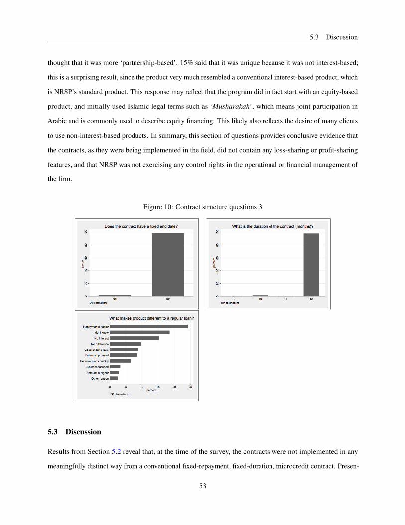
5.3 Discussion
thought that it was more ‘partnership-based’. 15% said that it was unique because it was not interest-based;
this is a surprising result, since the product very much resembled a conventional interest-based product, which
is NRSP’s standard product. This response may reflect that the program did in fact start with an equity-based
product, and initially used Islamic legal terms such as ‘Musharakah’, which means joint participation in
Arabic and is commonly used to describe equity financing. This likely also reflects the desire of many clients
to use non-interest-based products. In summary, this section of questions provides conclusive evidence that
the contracts, as they were being implemented in the field, did not contain any loss-sharing or profit-sharing
features, and that NRSP was not exercising any control rights in the operational or financial management of
the firm.
Figure 10: Contract structure questions 3
5.3 Discussion
Results from Section 5.2 reveal that, at the time of the survey, the contracts were not implemented in any
meaningfully distinct way from a conventional fixed-repayment, fixed-duration, microcredit contract. Presen-
53

5.3 Discussion
tation of results and a detailed focus group with senior managers and field officers revealed interesting reasons
for which these contracts, which had in fact started with performance-contingent repayments, converged
to a standard debt structure. Results relate to many of the themes that arise in earlier theoretical work on
sharecropping and income-sharing contracts, which suggest the optimality of a standard debt contract in the
presence of information asymmetries and costly state verification.37
I presented results from the survey to NRSP’s CEO, senior management and regional managers, with a
detailed focus-group-style discussion taking place over the course of three hours. There are two major
insights arising out of post-survey reflections and accounts from managers and field officers. First, from the
supply side, one valuable lesson is the difficulty in implementing equity-like contracts within the structure of
a conventional microcredit organisation. Loan officers did not have much incentive to finance higher-return,
higher-risk microenterprise owners by providing them with an unfamiliar product that required greater
monitoring effort and contained loss-sharing, especially because the loan officer would not themselves benefit
from the upside portion of the profit- and loss-sharing arrangement (i.e. they had no ‘skin in the game’).
Further, loan officers reported that it was very time-consuming to calculate profit- and loss-sharing amounts,
since many microenterprises did not keep adequate income statements, thereby requiring the loan officer to
essentially create these. Even when records were kept, they were often paper-based and took much time to
process for calculating performance-contingent payments, which reinforces the idea that in a world of costly
state verification, a non-performance-contingent contract may be optimal.
The second key lesson arising out of post-survey interviews was from the perspective of clients. Results
indicate that many clients had serious objections to the sharing rule used in the contracts when they were
originally implemented with profit- and loss-sharing. A common sharing rule led to the most profitable
entrepreneurs having to share too much of their profits and thus the equity product, ironically, appearing to be
very ‘inequitable’ to them. The post-survey focus group with NRSP management revealed that gradually
this led to loan officers and clients mutually agreeing to remove the performance-contingent aspect of the
contracts, which eventually converged to a fixed-repayment structure, albeit on much more lenient terms37 See Townsend (1979); Stiglitz and Weiss (1981).
54

5.3 Discussion
than a conventional microcredit contract. Had NRSP maintained performance-contingent contracts alongside
fixed-repayment contracts, adverse selection may have become a serious issue, with the most profitable
microenterprises deciding to re-negotiate to a debt contract, and the least profitable ones remaining on
performance-contingent contracts. Hence, the decision taken by NRSP management to revert all contracts
back to a standard fixed repayment schedule appears to have been appropriate. This decision to move back
to debt-like contracts also appears prudent in light of the potential adverse consequences of moral hazard.
Since a 20-80 sharing ratio was considered inappropriate by some of the more profitable businesses, in that
they were obliged to share too much of their profits, had NRSP not renegotiated the contract then it could
have created negative incentives for those microenterprises stuck on ‘unfair’ sharing ratios. This may have
encouraged them either to exert less effort – for instance if they equated their marginal disutility of effort
with their share of their marginal product rather than total marginal product – or to simply understate their
profits, which would be difficult to detect due to costly state verification.
Intriguingly, NRSP branch managers also observed that, even though the contracts originally maintained a
‘downside option’ that did allow for loss-sharing ex-ante, in practice no entrepreneurs ever exercised this
loss-sharing option. This was due to a fear that if they did not meet their expected payment every month, it
would adversely affect their standing with the bank, which may hinder their ability to borrow in the future.
Therefore, fears regarding reputation and dynamic incentives actually led to microenterprise owners not
exercising their loss-sharing option, even when NRSP had explicitly allowed it. In summary, these findings
from the survey of NRSP clients suggest that it is very challenging to implement equity-based contracts
within a conventional microcredit organisation. The major constraints relate to the incentives of microcredit
loan officers and those of clients, as discussed in earlier theoretical work on optimal financial contracts in
the presence of asymmetric information and costly state verification. These are compounded by the related
problems of adverse selection (the most profitable microenterprises selecting out of equity contracts) and
moral hazard (distortionary effects caused by inappropriately chosen income-sharing ratios).
55

Conclusion
6 Conclusion
Access to finance is frequently listed as one of the most important constraints on the expansion of small firms
in low-income countries. Many existing studies focus on the role of microcredit as a source of capital; other
work complements this by considering the potential effect of microsavings and microinsurance. In this paper,
I investigate the effect of ‘microequity’ contracts, which provide capital using a performance-contingent
repayment schedule that allows a greater sharing of risk and reward between capital provider and microenter-
prise. In the first part of the paper, I describe the implementation of an artefactual field experiment, designed
using a simple model of investment choice under different financial contracts, and tested with microenterprise
owners who are part of a large field experiment that provides them with a graduated loan to expand their
business with a fixed asset. Results reveal that equity-financed microentrepreneurs chose investment options
with a greater expected return and risk than under debt financing, with heterogeneity analysis showing a
larger effect for more risk- and loss-averse microenterprise owners. In the second part of the paper, I explore
the question of why microequity contracts do not appear to be part of the current portfolio of products offered
by most microfinance institutions, considering the significant potential benefits identified in the first part
of the paper. To shed some light on this question, I report on an attempt by one of the largest microfinance
institutions in Pakistan to implement equity-based microfinance contracts with microenterprise owners in the
field. Results from a detailed client survey and a post-survey focus group with senior management point to the
significant challenges of implementing equity-based contracts within a conventional microcredit organisation,
with the major constraints relating both to the incentives for microcredit loan officers as well as costly state
verification, adverse selection and moral hazard.
56

Appendix
7 Appendix
Table 15: Simulations: Changing the number of game rounds.
This figure presents results from simulations with a different number of investment rounds in the game: (beginning in the top-left panel, goingclockwise): 3, 5, 7 and 10 rounds.
57
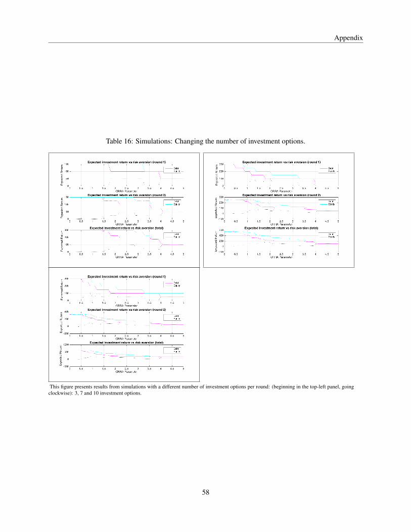
Appendix
Table 16: Simulations: Changing the number of investment options.
This figure presents results from simulations with a different number of investment options per round: (beginning in the top-left panel, goingclockwise): 3, 7 and 10 investment options.
58

Appendix
Table 17: Simulations: Changing the initial wealth level in the game.
This figure presents results from simulations with a different starting amount of investment wealth in the first round of the game: (beginning inthe top-left panel, going clockwise): 100, 300, 500, and 700.
59
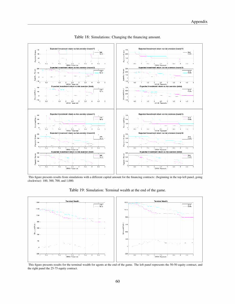
Appendix
Table 18: Simulations: Changing the financing amount.
This figure presents results from simulations with a different capital amount for the financing contracts: (beginning in the top-left panel, goingclockwise): 100, 300, 700, and 1,000.
Table 19: Simulation: Terminal wealth at the end of the game.
This figure presents results for the terminal wealth for agents at the end of the game. The left panel represents the 50-50 equity contract, andthe right panel the 25-75 equity contract.
60

Appendix
Figure 11: Business Performance Metrics
Figure 12: Background of apprentices and how the funds were used.
61

REFERENCES
References
ANGELUCCI, M., D. KARLAN, and J. ZINMAN (2015): “Microcredit impacts: Evidence from a randomized
microcredit program placement experiment by Compartamos Banco”. American Economic Journal:
Applied Economics 7.1, pp. 151–82.
ATTANASIO, O., B. AUGSBURG, R. DE HAAS, E. FITZSIMONS, and H. HARMGART (2015): “The
impacts of microfinance: Evidence from joint-liability lending in Mongolia”. American Economic Journal:
Applied Economics 7.1, pp. 90–122.
AUGSBURG, B., R. DE HAAS, H. HARMGART, and C. MEGHIR (2015): “The impacts of microcredit:
Evidence from Bosnia and Herzegovina”. American Economic Journal: Applied Economics 7.1, pp. 183–
203.
AYYAGARI, M., T. BECK, and A. DEMIRGUC-KUNT (2007): “Small and medium enterprises across the
globe”. Small business economics 29.4, pp. 415–434.
BANERJEE, A., D. KARLAN, and J. ZINMAN (2015): “Six randomized evaluations of microcredit:
Introduction and further steps”. American Economic Journal: Applied Economics 7.1, pp. 1–21.
BARBONI, G. (2017): “Repayment flexibility in microfinance contracts: Theory and experimental evidence
on take up and selection”. Journal of Economic Behavior & Organization 142, pp. 425–450.
BARR, A. and T. G. PACKARD (2002): “Revealed Preference and Self-insurance: Can we learn from the
Self-employed in Chile?” Working paper.
BARTLING, B., E. FEHR, and H. HERZ (2014): “The intrinsic value of decision rights”. Econometrica 82.6,
pp. 2005–2039.
BATTAGLIA, M., S. GULESCI, and A. MADESTAM (2017): “Contractual Flexibility, Firm Growth, and
Information Asymmetries in Microfinance: Experimental Evidence from Bangladesh”. Working paper.
BECK, T., A. DEMIRGÜÇ-KUNT, and M. S. MARTINEZ PERIA (2008): “Banking services for everyone?
Barriers to bank access and use around the world”. The World Bank Economic Review 22.3, pp. 397–430.
62

REFERENCES
BELLONI, A., V. CHERNOZHUKOV, and C. HANSEN (2014): “High-dimensional methods and inference
on structural and treatment effects”. Journal of Economic Perspectives 28.2, pp. 29–50.
BINSWANGER, H. P. (1981): “Attitudes toward risk: Theoretical implications of an experiment in rural
India”. The Economic Journal 91.364, pp. 867–890.
BLOOM, N. and J. VAN REENEN (2010): “Why do management practices differ across firms and countries?”
Journal of economic perspectives 24.1, pp. 203–24.
CHARNESS, G., U. GNEEZY, and B. HALLADAY (2016): “Experimental methods: Pay one or pay all”.
Journal of Economic Behavior & Organization 131, pp. 141–150.
CRÉPON, B., F. DEVOTO, E. DUFLO, and W. PARIENTÉ (2015): “Estimating the impact of microcredit
on those who take it up: Evidence from a randomized experiment in Morocco”. American Economic
Journal: Applied Economics 7.1, pp. 123–50.
DE MEL, S., D. MCKENZIE, and C. WOODRUFF (2008): “Returns to capital in microenterprises: evidence
from a field experiment”. The quarterly journal of Economics 123.4, pp. 1329–1372.
DOHMEN, T., A. FALK, D. HUFFMAN, U. SUNDE, J. SCHUPP, and G. G. WAGNER (2011): “Individual
risk attitudes: Measurement, determinants, and behavioral consequences”. Journal of the European
Economic Association 9.3, pp. 522–550.
DUFLO, E., A. BANERJEE, R. GLENNERSTER, and C. G. KINNAN (2013): The miracle of microfinance?
Evidence from a randomized evaluation. Tech. rep. National Bureau of Economic Research.
FAFCHAMPS, M., D. MCKENZIE, S. QUINN, and C. WOODRUFF (2014): “Microenterprise growth
and the flypaper effect: Evidence from a randomized experiment in Ghana”. Journal of development
Economics 106, pp. 211–226.
FIELD, E., R. PANDE, J. PAPP, and N. RIGOL (2013): “Does the classic microfinance model discourage
entrepreneurship among the poor? Experimental evidence from India”. American Economic Review 103.6,
pp. 2196–2226.
FISCHER, G. (2013): “Contract Structure, Risk-Sharing, and Investment Choice”. Econometrica 81.3,
pp. 883–939.
63

REFERENCES
EL-GAMAL, M., M. EL-KOMI, D. KARLAN, and A. OSMAN (2014): “Bank-insured RoSCA for microfi-
nance: Experimental evidence in poor Egyptian villages”. Journal of Economic Behavior & Organization
103, S56–S73.
GINÉ, X., P. JAKIELA, D. KARLAN, and J. MORDUCH (2010): “Microfinance games”. American Eco-
nomic Journal: Applied Economics 2.3, pp. 60–95.
HARRISON, G. W. and E. ELISABET RUTSTRÖM (2008): “Risk aversion in the laboratory”. Risk aversion
in experiments. Emerald Group Publishing Limited, pp. 41–196.
HOLT, C. A. and S. K. LAURY (2002): “Risk aversion and incentive effects”. American economic review
92.5, pp. 1644–1655.
KAMMER, M. A., M. M. NORAT, M. M. PINON, A. PRASAD, M. C. M. TOWE, and M. Z. ZEIDANE
(2015): Islamic finance: Opportunities, challenges, and policy options. 15. International Monetary Fund.
KARLAN, D. and J. ZINMAN (2011): “Microcredit in theory and practice: Using randomized credit scoring
for impact evaluation”. Science 332.6035, pp. 1278–1284.
EL-KOMI, M. and R. CROSON (2013): “Experiments in Islamic microfinance”. Journal of Economic
Behavior & Organization 95, pp. 252–269.
LEVITT, S. D. and J. A. LIST (2007): “What do laboratory experiments measuring social preferences reveal
about the real world?” Journal of Economic perspectives 21.2, pp. 153–174.
MCKENZIE, D. and C. WOODRUFF (2016): “Business practices in small firms in developing countries”.
Management Science 63.9, pp. 2967–2981.
MEAGER, R. (2018): “Understanding the Average Impact of Microcredit Expansions: A Bayesian Hierarchi-
cal Analysis of Seven Randomized Experiments”. American Economic Journal: Applied Economics.
MULLAINATHAN, S. and J. SPIESS (2017): “Machine learning: an applied econometric approach”. Journal
of Economic Perspectives 31.2, pp. 87–106.
NIMRAH, K., T. MICHAEL, and R. XAVIER (2008): “Islamic microfinance: An emerging market niche”.
Focus Note 49.
64

REFERENCES
OBAIDULLAH, M. and T. KHAN (2008): “Islamic microfinance development: Challenges and initiatives”.
STEIN, P., O. P. ARDIC, and M. HOMMES (2013): “Closing the credit gap for formal and informal micro,
small, and medium enterprises”. International Finance Corporation.
STIGLITZ, J. and A. WEISS (1981): “Credit rationing in markets with imperfect information”. The American
economic review 71.3, pp. 393–410.
TAROZZI, A., J. DESAI, and K. JOHNSON (2015): “The impacts of microcredit: Evidence from Ethiopia”.
American Economic Journal: Applied Economics 7.1, pp. 54–89.
TOWNSEND, R. M. (1979): “Optimal contracts and competitive markets with costly state verification”.
Journal of Economic theory 21.2, pp. 265–293.
VIEIDER, F. M., M. LEFEBVRE, R. BOUCHOUICHA, T. CHMURA, R. HAKIMOV, M. KRAWCZYK,
and P. MARTINSSON (2015): “Common components of risk and uncertainty attitudes across contexts
and domains: Evidence from 30 countries”. Journal of the European Economic Association 13.3, pp. 421–
452.
WORLD BANK, T. (2012): “Islamic Finance - A Catalyst for Shared Prosperity?” World Bank.
65

Designed by soapbox.co.uk
The International Growth Centre (IGC) aims to promote sustainable growth in developing countries by providing demand-led policy advice based on frontier research.
Find out more about our work on our website www.theigc.org
For media or communications enquiries, please contact [email protected]
Subscribe to our newsletter and topic updates www.theigc.org/newsletter
Follow us on Twitter @the_igc
Contact us International Growth Centre, London School of Economic and Political Science, Houghton Street, London WC2A 2AE