MICRO-SIMULATION OF THE ROUNDABOUT AT IDROTTSPARKEN USING AIMSUN551346/FULLTEXT03.pdf ·...

LiU-ITN-TEK-A--12/051--SE

MICRO-SIMULATION OF THE ROUNDABOUT AT

IDROTTSPARKEN USING AIMSUN

A Case Study of Idrottsparken Roundabout in Norrköping, Sweden

SEPTARINA

Linköping University Department of Science and Technology

Intelligent Transport System 2012

iii

LiU-ITN-TEK-A--12/051--SE

MICRO-SIMULATION OF THE ROUNDABOUT AT

IDROTTSPARKEN USING AIMSUN

A Case Study of Idrottsparken Roundabout in Norrköping, Sweden

Submitted in partial fulfillment of the requirements for the degree of Master of Science in the Department of Science and Technology

Programme of Intelligent Transport System Linköping University

SEPTARINA

EXAMINATOR CLAS RYDERGREN

Norrköping 6/23/2012

iv

COPYRIGHT

The publishers will keep this document online on the Internet – or its possible replacement –from the date of publication barring exceptional circumstances.

The online availability of the document implies permanent permission for anyone to read, to download, or to print out single copies for his/hers own use and to use it unchanged for non-commercial research and educational purpose. Subsequent transfers of copyright cannot revoke this permission. All other uses of the document are conditional upon the consent of the copyright owner. The publisher has taken technical and administrative measures to assure authenticity, security and accessibility.

According to intellectual property law the author has the right to be mentioned when his/her work is accessed as described above and to be protected against infringement.

For additional information about the Linköping University Electronic Press and its procedures for publication and for assurance of document integrity, please refer to its www home page: http://www.ep.liu.se/.

© Septarina

v

ABSTRACT

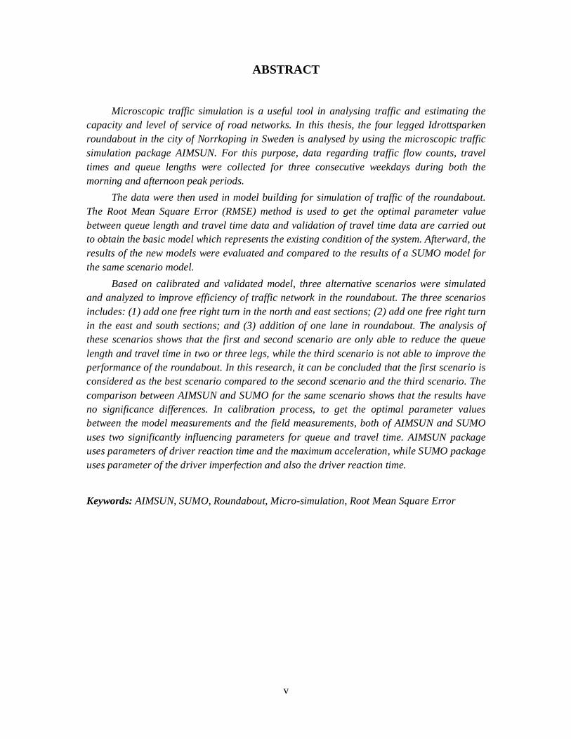
Microscopic traffic simulation is a useful tool in analysing traffic and estimating the capacity and level of service of road networks. In this thesis, the four legged Idrottsparken roundabout in the city of Norrkoping in Sweden is analysed by using the microscopic traffic simulation package AIMSUN. For this purpose, data regarding traffic flow counts, travel times and queue lengths were collected for three consecutive weekdays during both the morning and afternoon peak periods.

The data were then used in model building for simulation of traffic of the roundabout. The Root Mean Square Error (RMSE) method is used to get the optimal parameter value between queue length and travel time data and validation of travel time data are carried out to obtain the basic model which represents the existing condition of the system. Afterward, the results of the new models were evaluated and compared to the results of a SUMO model for the same scenario model.

Based on calibrated and validated model, three alternative scenarios were simulated and analyzed to improve efficiency of traffic network in the roundabout. The three scenarios includes: (1) add one free right turn in the north and east sections; (2) add one free right turn in the east and south sections; and (3) addition of one lane in roundabout. The analysis of these scenarios shows that the first and second scenario are only able to reduce the queue length and travel time in two or three legs, while the third scenario is not able to improve the performance of the roundabout. In this research, it can be concluded that the first scenario is considered as the best scenario compared to the second scenario and the third scenario. The comparison between AIMSUN and SUMO for the same scenario shows that the results have no significance differences. In calibration process, to get the optimal parameter values between the model measurements and the field measurements, both of AIMSUN and SUMO uses two significantly influencing parameters for queue and travel time. AIMSUN package uses parameters of driver reaction time and the maximum acceleration, while SUMO package uses parameter of the driver imperfection and also the driver reaction time.

Keywords: AIMSUN, SUMO, Roundabout, Micro-simulation, Root Mean Square Error

vii

ACKNOWLEDGMENTS

Praise and thanks to Allah the Al-Mighty, the Most Gracious, the Most Merciful for the grace, blessing, guidance, gift of love and talent in my life.

This thesis is written in order to fulfill the requisite of Master Programme in Department of Science and Technology, Programme of Intelligent Transport System, Linkoping University and Master Programme in Transportation System and Engineering and Environment Department, Faculty of Engineering, Gadjah Mada University. The author would like to express her gratitude to those who have contributed to this thesis. Without their support and encouragement, the completion of this thesis would not have happened.

Many thanks to my examiner Clas Rydergren, Ph.D and Prof. Jan Lundgren from Linkoping University, and also Prof. Dr. Ir. Siti Malkhamah, M.Sc. and Ir. Wardhani Sartono, M.Sc. from Gadjah Mada University for their guidance and invaluable feedback in this research.

Thanks to the lecturers and staffs in postgraduate programme in Transport System and Engineering, Gadjah Mada University and Intelligent Transport System, Linkoping University, Sweden. Not to forget my classmates in batch XXII MSTT UGM and colleagues in Linkoping University, Sweden.

I would like to express my sincere thanks to my parents and to my family. Thank you for support, prayer, love and encouragement. Thanks to all my friends; Catur, Aji, Taufiq and Tina for their support in collection data process.

This thesis still needs to be improved. Any suggestion and critic from the reader is appreciated as an input to refine for further study.

Norrkoping, 23 June 2012

SEPTARINA

ix

LIST OF ABBREVIATIONS

AIMSUN : Advanced Interactive Microscopic Simulator for Urban and Non-urban Network

CORSIM : CORridor-microscopic SIMulation program

DLR : Deutsches Zentrum für Luft- und Raumfahrt e.V (German for German Aerospace Center)

FHWA : The Federal Highway Administration

KYTC : Kentucky Transportation Cabinet

MKJI : Manual Kapasitas Jalan Indonesia (Indonesia for the Indonesia Road Capacity Manual)

MSE : Mean Square Error

NAASRA : National Association of Australian State Road Authorities

O-D : Origin - Destination

PARAMICS : Parallel Microscopic Simulation

pcu : Passenger Car Unit

SUMO : Simulation for Urban Mobility

RMSE : Root Mean Square Error

TRRL : Transport and Road Research Laboratory

TSS : Transport Simulation System

VISSIM : Verkehr In Städten - SIMulationsmodell (German for “Traffic in cities - simulation model)

XML : Extensible Markup Language

2-D : 2 Dimensional

3-D : 3 Dimensional

xi

TABLE OF CONTENTS

Page

COPYRIGHT ............................................................................................................................ iv

ABSTRACT ............................................................................................................................... v

ACKNOWLEDGMENTS ........................................................................................................ vii

LIST OF ABBREVIATIONS ................................................................................................... ix

LIST OF TABLES .................................................................................................................. xiii

LIST OF FIGURES .................................................................................................................. xv

I. INTRODUCTION ............................................................................................................... 1

I.1. Background ................................................................................................................ 1

I.2. Project Aim and Purpose ........................................................................................... 2

I.3. Limitation................................................................................................................... 2

I.4. Previous Researches .................................................................................................. 2

II. LITERATURE REVIEW AND THEORETICAL BASE .................................................. 5

II.1. Simulation Model Using AIMSUN ........................................................................... 5

II.2. Roundabouts .............................................................................................................. 6

II.3. Calibration ................................................................................................................. 7

II.3.1. Select calibration parameters ......................................................................... 7

II.3.2. Optimal parameter value ................................................................................ 7

II.4. Validation................................................................................................................... 8

III. RESEARCH METHODOLOGY ...................................................................................... 11

III.1. Research Location.................................................................................................... 11

III.2. Micro-simulation Model Process ............................................................................. 11

III.3. Data Collection ........................................................................................................ 14

III.3.1. Road inventory ............................................................................................. 15

III.3.2. Traffic flow count ........................................................................................ 16

III.3.3. Queue survey ............................................................................................... 18

III.3.4. Travel time measurements ........................................................................... 19

IV. MODELING AND SIMULATION .................................................................................. 21

IV.1. Base Model Development ........................................................................................ 21

IV.2. Error Checking ......................................................................................................... 22

IV.3. Calibration Process .................................................................................................. 23

xii

IV.3.1. Model parameter setting............................................................................... 23

IV.3.2. Optimal Parameter Value ............................................................................. 23

IV.4. Validation Process ................................................................................................... 28

V. ALTERNATIVE SCENARIOS ........................................................................................ 35

V.1. Alternative Scenario 1: Free right turn implementation (on North and East sections) ................................................................................................................... 35

V.2. Alternative Scenario 2: Free right turn implementation (on East and South sections) ................................................................................................................... 36

V.3. Alternative Scenario 3: Addition of lane in roundabout .......................................... 37

VI. RESULT AND ANALYSIS ............................................................................................. 39

VI.1. Scenario 1 ................................................................................................................ 39

VI.2. Scenario 2 ................................................................................................................ 43

VI.3. Scenario 3 ................................................................................................................ 46

VI.4. Comparison of Performance Results ....................................................................... 50

VI.5. Comparison Between AIMSUN and SUMO ........................................................... 53

VI.5.1. System properties ......................................................................................... 53

VI.5.2. Simulation result .......................................................................................... 54

VII. CONCLUSION ................................................................................................................. 59

REFERENCES ......................................................................................................................... 61

APPENDIX 1. PRELIMINARY SURVEY ........................................................................... A-1

APPENDIX 2. TRAFFIC FLOW COUNT ............................................................................ A-3

APPENDIX 3. MEAN OF MAXIMUM QUEUE LENGTH ................................................ A-7

APPENDIX 4. MEAN OF TRAVEL TIME .......................................................................... A-8

APPENDIX 5. OUTPUT SIMULATION ............................................................................. A-9

APPENDIX 6. DOCUMENTATION .................................................................................. A-13

xiii

LIST OF TABLES page

Table 3.1. Schedule of survey .............................................................................................. 15

Table 3.2. Traffic flow count per section in morning .......................................................... 16

Table 3.3. Traffic flow count per section in afternoon ........................................................ 17

Table 3.4. Turning proportion per type of vehicle in morning ............................................ 17

Table 3.5. Turning proportion per type of vehicle in afternoon ........................................... 18

Table 3.6. Queue length in morning..................................................................................... 18

Table 3.7. Queue length in afternoon ................................................................................... 19

Table 3.8. Travel time in morning ....................................................................................... 19

Table 3.9. Travel time in afternoon ...................................................................................... 19

Table 4.1. Input coding error checking ................................................................................ 22

Table 4.2. The RMSE combination between the maximum queue length and travel time in morning ................................................................................................... 25

Table 4.3. The RMSE combination between the maximum queue length and travel time in afternoon ................................................................................................. 27

Table 4.4. Calibrated model parameter ................................................................................ 28

Table 4.5. Result for validation model in morning (driver reaction time = 0.65 and max acceleration: max = 3, mean = 2.5, min = 2)............................................... 28

Table 4.6. Result for validation model in morning (driver reaction time = 0.65 and max acceleration: max = 1, mean = 1, min = 1) ................................................. 29

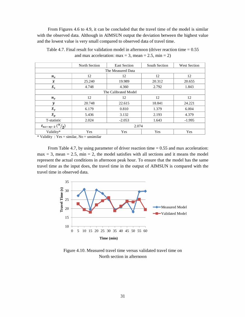
Table 4.7. Final result for validation model in afternoon (driver reaction time = 0.55 and max acceleration: max = 3, mean = 2.5, min = 2) ........................................ 31

Table 6.1. Comparison of the mean of maximum queue length and travel time

between scenario 1 and the validated model in morning .................................... 40

Table 6.2. The mean of maximum queue length and travel time t-test between scenario 1 and the validated model in morning .................................................. 40

Table 6.3. Comparison of the mean of maximum queue length and travel time between scenario 1 and the validated model in afternoon .................................. 42

Table 6.4. The mean of maximum queue length and travel time t-test between scenario 1 and the validated model in afternoon ................................................. 42

Table 6.5. Comparison of the mean of maximum queue length and travel time between scenario 2 and the validated model in morning .................................... 43

Table 6.6. The Mean of maximum queue length and travel time t- test between scenario 2 and the validated model in morning .................................................. 44

Table 6.7. Comparison of the mean of maximum queue length and travel time between scenario 2 and the validated model in afternoon .................................. 45

xiv

Table 6.8. The Mean of maximum queue length and travel time t-test between scenario 2 and the validated model in afternoon ................................................. 46

Table 6. 9. Comparison of the mean of maximum queue length and travel time between scenario 3 and the validated model in morning .................................... 47

Table 6.10. The mean of maximum queue length and travel time t-test between scenario 3 and the validated model in morning .................................................. 48

Table 6.11. Comparison of mean of queue length and travel time between scenario 3 and the validated model in afternoon .................................................................. 49

Table 6.12. The mean of maximum queue length and travel time t-test between scenario 3 and the validated model in afternoon ................................................. 50

Table 6.13. Comparison of system properties between AIMSUN and SUMO ..................... 54

xv

LIST OF FIGURES Page

Figure 2.1. Basic geometric elements of a roundabout (FHWA, 2000) .................................. 7

Figure 3.1. Street View of the Idrottsparken Roundabout (Bing Maps, 2010) ..................... 11

Figure 3.2. Micro-simulation model development and application process ......................... 13

Figure 3.3. Surveyor position ................................................................................................ 14

Figure 3.4. The dimension of the Idrottsparken roundabout ................................................. 16

Figure 4.1. Project model simulation .................................................................................... 21

Figure 4.2. Minimization of RMSE between the model output and the field measurements by using maximum queue length data in morning ...................... 23

Figure 4.3. Minimization of RMSE between the model output and the field measurements by using travel time data in morning ........................................... 24

Figure 4.4. Minimization of RMSE between the model output and the field measurements by using maximum queue length data in afternoon .................... 26

Figure 4.5. Minimization of RMSE between the model output and the field measurements by using travel time data in afternoon ......................................... 26

Figure 4.6. Measured travel time versus validated travel time on North section in morning ............................................................................................................... 29

Figure 4.7. Measured travel time versus validated travel time on East section in morning ............................................................................................................... 30

Figure 4.8. Measured travel time versus validated travel time on South section in morning ............................................................................................................... 30

Figure 4.9. Measured travel time versus validated travel time on West section in morning ............................................................................................................... 30

Figure 4.10. Measured travel time versus validated travel time on North section in afternoon ............................................................................................................. 31

Figure 4.11. Measured travel time versus validated travel time on East section in afternoon ............................................................................................................. 32

Figure 4.12. Measured travel time versus validated travel time on South section in afternoon ............................................................................................................. 32

Figure 4.13. Measured travel time versus validated travel time on West section in afternoon ............................................................................................................. 32

Figure 5. 1. Free right turn implementation on North and East sections................................ 36

Figure 5.2. Free right turn implementation on East and South sections ................................ 37

Figure 5.3. Addition of lane in roundabout ........................................................................... 38

xvi

Figure 6.1. Mean of maximum queue length between scenario 1 and the validated model in morning ................................................................................................ 39

Figure 6.2. Mean of travel time between scenario 1 and the validated model in morning ............................................................................................................... 39

Figure 6.3. Mean of maximum queue length between scenario 1 and the validated model in afternoon .............................................................................................. 41

Figure 6.4. Mean of travel time between scenario 1 and the validated model in afternoon ............................................................................................................. 41









Figure 6.13. The percentage of the maximum queue length between Scenario 1, 2 and 3 in morning ........................................................................................................... 51

Figure 6.14. The percentage of travel time between Scenario 1, 2 and 3 in morning ............. 51

Figure 6.15. The percentage of the maximum queue length between Scenario 1, 2 and 3 in afternoon ......................................................................................................... 52

Figure 6.16. The percentage of the maximum queue length between Scenario 1, 2 and 3 in afternoon ......................................................................................................... 52

Figure 6.17. The percentage of the maximum queue length between AIMSUN model and SUMO model in morning ............................................................................. 55

Figure 6.18. The percentage of travel time between AIMSUN model and SUMO model in morning ........................................................................................................... 55

Figure 6.19. The percentage of the maximum queue length between AIMSUN model and SUMO model in afternoon ........................................................................... 56

Figure 6.20. The percentage of travel time between AIMSUN model and SUMO model in afternoon ......................................................................................................... 56

1

I. INTRODUCTION

With rapid urbanisation and the consequent growth of vehicle population, the urban roads are becoming more and more congested day by day. This necessitates the application of advanced technologies in the planning, design and operation of road traffic networks in order to ensure smooth flow of traffic. With the advent of computing technologies in the last few decades, a broad horizon has opened regarding the application of innovative tools like computer simulation for the planning, design and operation of road networks. Microscopic traffic simulation, which is one of the approaches of simulating road traffic, is defined as the one where individual vehicles are modelled as separate entities in order to assess the performance of the overall system. By using this type of simulation models, practitioners and transportation engineers will be able to create analysis with reliable data on the situation and the problem of the existing transportation system and focus on improving traffic performance by generating and evaluating the relevant measures to find the best alternative.

In many European countries, roundabouts have become more popular over the last decades in improving traffic performance and also reduce the number of accidents acting as a traffic calming device. Roundabouts have proved to be a safer alternative at intersection for both motor vehicles and pedestrians (FHWA, 2000). In recent years, traffic simulation method has been used to study the performance of not only signalised junctions, but also unsignalised junctions like roundabouts. Simulation is widely accepted as a useful technique to provide an experimental test in terms of comparing the alternate system design, replacing the experiments on the physical system by experiments on its formal depiction in a computer. The result can be the basis for a quantitive support to decision-makers. Based on this concept, the simulation model is used to carry out experiments on a model of the system to draw valid conclusion for the real system (TSS, 2010).

There are a number of commercially available microscopic traffic simulation packages such as CORSIM (USA), PARAMICS (UK), AIMSUN (Spain), SUMO and VISSIM (Germany). Among these packages, this research uses AIMSUN to build, calibrate and validate the model. This project presents an overview of the model building process of an AIMSUN model for an urban area.

I.1. Background

The roundabout at Idrottsparken connects three main streets at Norrkoping city, namely Kungsgatan (North section), Albrektsvägen (South section) and Södra Promenaden (West and East section). An observation of the performance of the streets shows that traffic congestions occur during the morning and evening peak hours. The streets are mainly affected by the vehicular and pedestrian trips generated through the activities from campus, sport stadium, business areas, shopping centre and industrial areas. The preliminary survey shows that significant queue builds up at each section of the roundabout during peak hours.

2

I.2. Project Aim and Purpose

The aim of the project is to build, calibrate, and validate a traffic model of the roundabout at Idrottsparken by using the microscopic traffic simulation software AIMSUN in order to experiment with a small reality traffic network. In addition, different sets of data, such as traffic flow, queue length and travel time will be used in calibration and validation processes in order to get more accurate results. Finally, alternative modifications were applied to improve efficiency of traffic network on the roundabout. The results of the new models were evaluated and compared to the results of a SUMO model for the same scenario model.

The purpose of the project is to combine the traffic simulation models with the statistical methods so it can be used to analyze the traffic problem.

I.3. Limitation

Some limitations encountered to make the project more focused and comprehensive are described as follows:

a. This project is using only the micro-simulation procedures of AIMSUN to analyse the traffic problem at the roundabout. Hence, the validity of the model depends on the validity of methodology associated with AIMSUN.

b. Traffic data collection is limited during the morning and afternoon peak hours, at 07.15-08.15 AM and 04.30-05.30 PM, while possibility remains that the peak period extends this period.

c. Problem assessment is solely focused on the roundabout at Idrottsparken without considering the minor junctions and side frictions along the street.

d. In this research, the subject is vehicles occupying the roundabout. The types of vehicles consist of passenger cars, buses and heavy vehicles (trucks). In field survey, the pedestrian and cyclist are not included believed not to significantly affect the traffic.

I.4. Previous Researches

Some previous researches related to micro simulation using AIMSUN package and its comparison with other softwares have carried out and published. The author made some review studies to compare the previous to the present research so that the author may combine and afford new hypothesis to analyze and solve the problem of this research. However, those researches differ in the focus of the discussions, objectives and case study.

G. Kotusevski and K.A. Hawick, 2009 have reviewed some of the traffic simulation software applications, the features and characteristics as well as the issues these applications performance, such as AIMSUN, PARAMICS, CORSIM and SUMO software. In this report, the authors analyzed that as traffic simulation software, AIMSUN were more user friendly than SUMO. In AIMSUN, to create traffic networks and associated vehicle patterns, the user

3

just simply using the available graphical network editor. While SUMO package, the user have to create manually (by hand) and write it in an XML file. The authors also found that pedestrian feature is available in AIMSUN, while SUMO package did not include this feature in its applications at all (Kotusevski & Hawick, 2009).

Jones et al., 2004 have compared some of the traffic simulation softwares. AIMSUN package was found to operate acceptably well compared to both SimTraffic and CORSIM packages and it possesses features that would be useful for creating large urban and regional networks. The dynamic traffic assignment capability is unmatched by either SimTraffic or CORSIM, but AIMSUN requires cumbersome coding (Jones et al., 2004).

Marjan Mosslemi, 2008 have applied a micro-simulation by using AIMSUN for roundabout with unbalanced flow pattern. This research is concluded that the capabilities of AIMSUN regarding traffic actuated control are enormously suitable and helpful for studying a variety of signalization and metering scenarios. This micro simulation package is strongly recommended as a powerful tool for later case studies of roundabout metering (Mosslemi, 2008).

In 2009, Mohsin Shahzad Chaudhry and Prakash Ranjitkar have conducted a micro-simulation model using AIMSUN to analyze the capacity and queue discharge flow rate at a signalized intersection. The research is concluded that AIMSUN is a viable tool for the evaluation and capacity analysis of a signalized intersection. However few limitations of AIMSUN were also observed during this research. These limitations are generally associated with editing and coding of the model. Among them the most important one is absence of the lane utilization factor (Chaudhry & Ranjitkar , 2009).

Manstetten et al., 1998 stated that the car following model in AIMSUN has been tested and calibrated in various research studies including research group from Robert Bosch Gmb H. The Bosch car-following test was conducted on different micro-simulation models commonly used in Europe and North America. The results in the test show that the AIMSUN car-following model was able to present fairly good replication of observed values (Manstetten et al., 1997).

In 2001, Malkhamah et al. have analyzed a roundabout in Bulaksumur, Yogyakarta by calculating the capacity and delay using three difference methods: Australia method (NAASRA 1986), UK method (TRRL) and Indonesia method (MKJI 1997). This study also analyzed the effect of driver behavior are not given priority when entering the roundabout will affect the capacity of the roundabout (Malkhamah et al., 2001).

Irvan Nurpandi, 2012 have evaluated a roundabout in Cianjur city in Indonesia using simulation of AIMSUN to know the expected performance. The research is concluded that the first alternative is not effective by changing the movement of the vehicle in the roundabout. While the second alternative gives a better and produces significant result by redesign of the roundabout (Nurpandi, 2012).

5

II. LITERATURE REVIEW AND THEORETICAL BASE

II.1. Simulation Model Using AIMSUN

AIMSUN is one of the microscopic traffic simulation software commonly used at present by transport professionals. The highly detailed model of traffic network and the specific difference of categorisation between the driver and vehicle type can be provided in this software. AIMSUN is able to simulate vehicles and pedestrians at the same time. Traffic equipment and control devices such as traffic light, traffic detector, variable message sign and ramp metering devices can also be modelled. Furthermore, the simulation model can be used to carry out experiments on a model of the system to draw valid conclusion for the real system (TSS, 2010). There are three principle parts for a simulation model in AIMSUN: the error checking, the calibration, and the validation processes.

The error checking step is essential in developing a working model. The succeeding steps of the calibration process rely on the elimination of all major errors in demand and network coding before calibration. In AIMSUN, there are three basic stages in the error checking procedure: (1) software error checking; (2) input coding error checking; and (3) animation review to spot less obvious input errors.

The calibration process is the adjustment of model parameters to improve the model’s ability to reproduce observed local driver behaviour and traffic performance characteristics. Without the calibration process, the analyst has no assurance that the model will accurately predict traffic performance for future scenarios. Validation is the process checking to determine whether the calibration result is valid to be used on field data to ensure the results are reasonable (FHWA, 2004).

In terms of calibration purposes, the AIMSUN vehicle modeling parameters can be classified into three groups according to their influence in the simulation output. The classifications are global parameters, local section parameters, and particular vehicle type parameters (TSS, 2010).

Global parameters give impacts on all vehicles while driving in the network without considering the vehicle type. Some examples of global parameters are reaction time, reaction time at stop, queue up and leaving speed, etc. Section parameters give impacts on all vehicles when driving in a certain section of the network without considering the type of vehicles. Some examples of local section parameters are speed limit, turning speed, visibility distance, etc. Vehicle parameters give impacts on all vehicles of particular type when driving anywhere in the network. Some examples of particular type parameters are maximum desired speed, maximum acceleration, normal and maximum deceleration, speed acceptance, minimum distance between vehicles, give-way time, and guidance acceptance.

6

II.2. Roundabouts

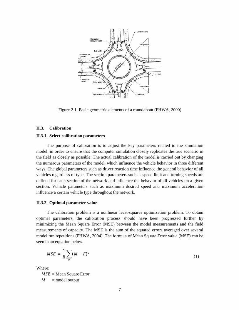
A roundabout is defined as a form of intersection design and control which accommodates traffic flow in one direction around a central island, operates with yield control at the entry points, and gives priority to vehicles within the roundabout (circulating flow). The main objective of roundabout design is to secure the safe interchange of traffic between crossing traffic streams with the minimum delay. Roundabouts have been categorized into six basic categories based on environment, number of lanes, and size. They are mini-roundabouts, urban compact roundabouts, urban single-lane roundabouts, urban double-lane roundabouts, rural single-lane roundabouts, and rural double-lane roundabouts (FHWA, 2000).

Roundabouts have considerable advantages in respect of their safety record because they can improve vehicle safety by eliminating or altering conflict points, reducing speed differentials at intersections, and forcing drivers to decrease speeds when enter to roundabout (FHWA, 2000). Roundabouts are particularly successful to increase traffic safety when the traffic flows are in balance on all approach legs, but they are a less effective form of intersection when the number of entry legs exceeds four. It mainly because of the size of the junction and the higher circulating speeds that can be achieved (FHWA, 2001).

There are three types of roundabout in Sweden: (1) mini, with inner radii R < 2 meters, requiring the center island to be fully traversable; small, with inner radii 2 < R < 10 meters, requiring the center island to be partly traversable; and (3) Normal, with inner radii R > l0, allowing for maneuver buses and trucks (Bergh, n.d.). According to this classification, the Idrottsparken roundabout is included into the classification of normal roundabout.

The optimal roundabout size, the optimal position, and the optimal alignment and arrangement of approach legs are three fundamental elements which must be determined in preliminary design of a roundabout. Design of double-lane roundabout is significantly different from design of single-lane roundabout. The techniques used in single-lane roundabout design do not directly transfer to double-lane design because designing the geometry of double-lane roundabouts is more complicated. Speeds through the roundabout, design vehicle, geometric elements, and the natural vehicle path have to be considered (FHWA, 2000).

7

Figure 2.1. Basic geometric elements of a roundabout (FHWA, 2000)

II.3. Calibration

II.3.1. Select calibration parameters

The purpose of calibration is to adjust the key parameters related to the simulation model, in order to ensure that the computer simulation closely replicates the true scenario in the field as closely as possible. The actual calibration of the model is carried out by changing the numerous parameters of the model, which influence the vehicle behavior in three different ways. The global parameters such as driver reaction time influence the general behavior of all vehicles regardless of type. The section parameters such as speed limit and turning speeds are defined for each section of the network and influence the behavior of all vehicles on a given section. Vehicle parameters such as maximum desired speed and maximum acceleration influence a certain vehicle type throughout the network.

II.3.2. Optimal parameter value

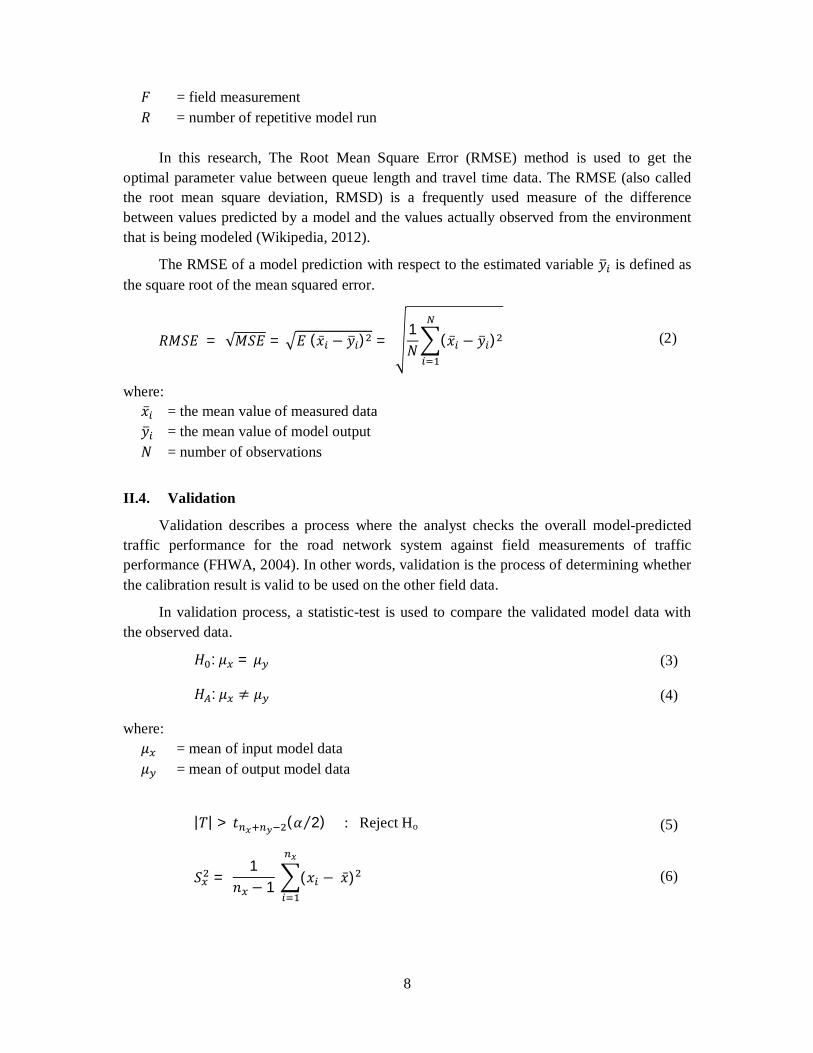
The calibration problem is a nonlinear least-squares optimization problem. To obtain optimal parameters, the calibration process should have been progressed further by minimizing the Mean Square Error (MSE) between the model measurements and the field measurements of capacity. The MSE is the sum of the squared errors averaged over several model run repetitions (FHWA, 2004). The formula of Mean Square Error value (MSE) can be seen in an equation below.

푀푆퐸 =1푅

(푀 −퐹) (1)

Where: 푀푆퐸 = Mean Square Error 푀 = model output

8

퐹 = field measurement 푅 = number of repetitive model run

In this research, The Root Mean Square Error (RMSE) method is used to get the optimal parameter value between queue length and travel time data. The RMSE (also called the root mean square deviation, RMSD) is a frequently used measure of the difference between values predicted by a model and the values actually observed from the environment that is being modeled (Wikipedia, 2012).

The RMSE of a model prediction with respect to the estimated variable 푦 is defined as the square root of the mean squared error.

푅푀푆퐸 = √푀푆퐸 = 퐸(푥̅ − 푦 ) = 1푁

(푥̅ − 푦 ) (2)

where: 푥̅ = the mean value of measured data 푦 = the mean value of model output 푁 = number of observations

II.4. Validation

Validation describes a process where the analyst checks the overall model-predicted traffic performance for the road network system against field measurements of traffic performance (FHWA, 2004). In other words, validation is the process of determining whether the calibration result is valid to be used on the other field data.

In validation process, a statistic-test is used to compare the validated model data with the observed data.

퐻 :휇 = 휇 (3)

퐻 :휇 ≠ 휇 (4)

where: 휇 = mean of input model data 휇 = mean of output model data

|푇| > 푡 (훼 2⁄ ) : Reject Ho (5)

푆 = 1

푛 − 1 (푥 − 푥̅) (6)

9

푆 = 1

푛 − 1 (푦 −푦) (7)

푠 =(푛 − 1)푠 + 푛 − 1 푠

푛 + 푛 − 2 (8)

푇 =푥̅ − 푦푠

푛 푛푛 + 푛

(9)

Where the 푡 (훼 2⁄ ) value is obtained from T-table, α is confidence interval, here set to 95% (α = 0.05), n is the total number of measured or modeled data, and S is standard deviation of measured or modeled data.

In the hypothesis test, the significance of the improvement of certain parameter in the new scenario (퐻 ) will be tested. The 퐻 will be rejected if 푇 < −푇 or 푇 > 푇 . It indicates that the data of the simulation is invalid or there is a significance differences between the simulation data and measured data.

11

III. RESEARCH METHODOLOGY

III.1. Research Location

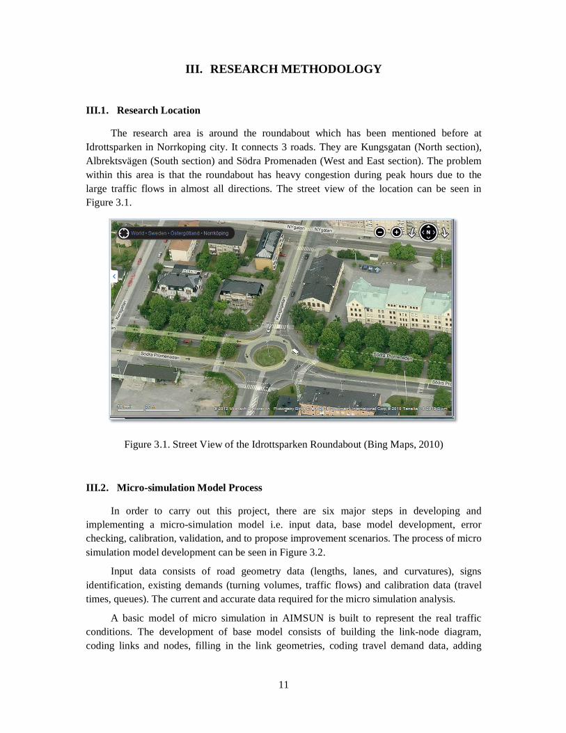
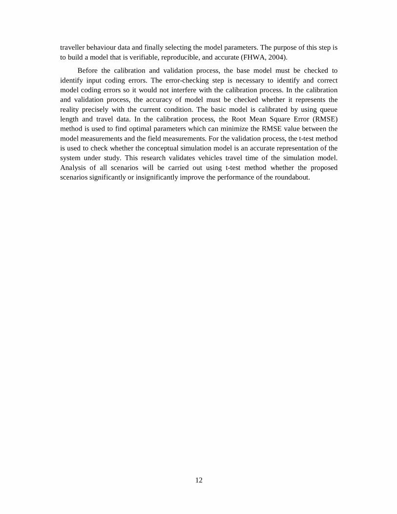
The research area is around the roundabout which has been mentioned before at Idrottsparken in Norrkoping city. It connects 3 roads. They are Kungsgatan (North section), Albrektsvägen (South section) and Södra Promenaden (West and East section). The problem within this area is that the roundabout has heavy congestion during peak hours due to the large traffic flows in almost all directions. The street view of the location can be seen in Figure 3.1.

Figure 3.1. Street View of the Idrottsparken Roundabout (Bing Maps, 2010)

III.2. Micro-simulation Model Process

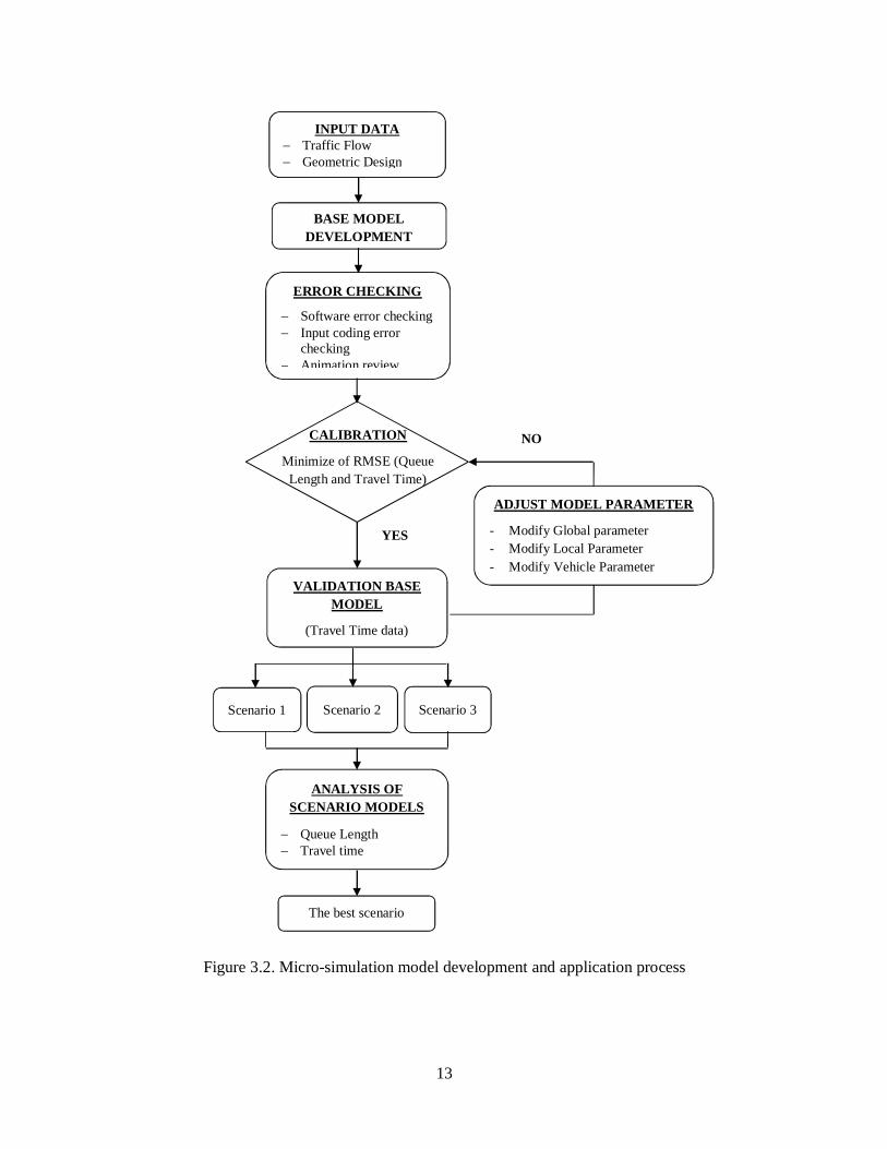
In order to carry out this project, there are six major steps in developing and implementing a micro-simulation model i.e. input data, base model development, error checking, calibration, validation, and to propose improvement scenarios. The process of micro simulation model development can be seen in Figure 3.2.

Input data consists of road geometry data (lengths, lanes, and curvatures), signs identification, existing demands (turning volumes, traffic flows) and calibration data (travel times, queues). The current and accurate data required for the micro simulation analysis.

A basic model of micro simulation in AIMSUN is built to represent the real traffic conditions. The development of base model consists of building the link-node diagram, coding links and nodes, filling in the link geometries, coding travel demand data, adding

12

traveller behaviour data and finally selecting the model parameters. The purpose of this step is to build a model that is verifiable, reproducible, and accurate (FHWA, 2004).

Before the calibration and validation process, the base model must be checked to identify input coding errors. The error-checking step is necessary to identify and correct model coding errors so it would not interfere with the calibration process. In the calibration and validation process, the accuracy of model must be checked whether it represents the reality precisely with the current condition. The basic model is calibrated by using queue length and travel data. In the calibration process, the Root Mean Square Error (RMSE) method is used to find optimal parameters which can minimize the RMSE value between the model measurements and the field measurements. For the validation process, the t-test method is used to check whether the conceptual simulation model is an accurate representation of the system under study. This research validates vehicles travel time of the simulation model. Analysis of all scenarios will be carried out using t-test method whether the proposed scenarios significantly or insignificantly improve the performance of the roundabout.

13

Figure 3.2. Micro-simulation model development and application process

NO

YES

CALIBRATION

Minimize of RMSE (Queue Length and Travel Time)

VALIDATION BASE MODEL

(Travel Time data)

BASE MODEL DEVELOPMENT

INPUT DATA Traffic Flow Geometric Design

ERROR CHECKING

Software error checking Input coding error

checking Animation review

Scenario 1 Scenario 3

ANALYSIS OF SCENARIO MODELS

Queue Length Travel time

The best scenario

Scenario 2

ADJUST MODEL PARAMETER

- Modify Global parameter - Modify Local Parameter - Modify Vehicle Parameter

14

III.3. Data Collection

Data collection is an important step in this project since the accurate and reliable data influences the quality of the AIMSUN model. This section discusses the types of data that needs to be used to build, calibrate and validate an AIMSUN model. It also describes the methods used in collecting these data. In this project, it was decided to collect following data: road inventory, traffic flow and turning movement count, queue length, and travel time.

Road inventory survey is conducted to collect some data related to speed limit and the geometry of the roundabout. Traffic flow is measured as the input of an OD-matrix for this project. It describes the total traffic flow entered to the roundabout from each direction. Moreover, it also gives the information of turning proportion for each direction. Queue length is a quite useful and intuitive parameter to describe the current situation of traffic congestion. This data is used for calibration process. For the type of data used for calibration and validation, travel time data is chosen.

A preliminary survey was conducted before subsequent surveys to get the data for modeling the traffic condition. This preliminary survey was done in order to find the traffic condition and to identify the peak hour. Based on the observation during the preliminary survey, the peak hour takes place at 07.15-08.15 AM in the morning and 04.30-05.30 PM in the afternoon. The result of the preliminary survey can be seen in Appendix 1.

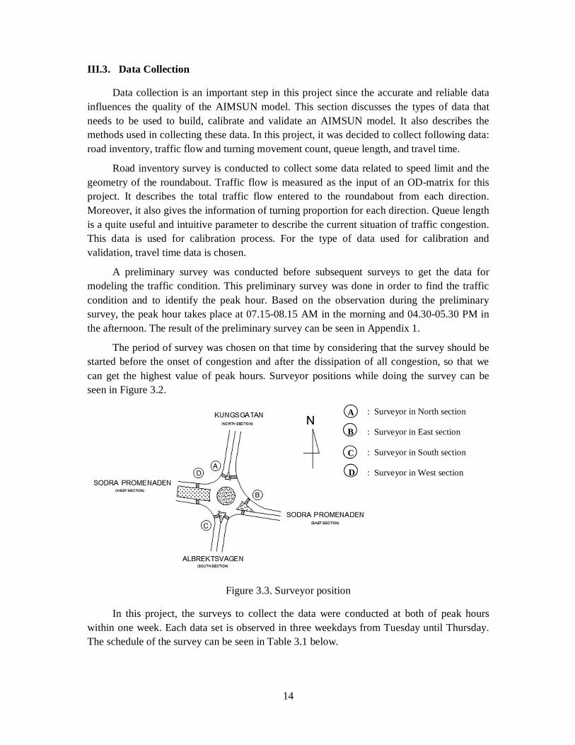
The period of survey was chosen on that time by considering that the survey should be started before the onset of congestion and after the dissipation of all congestion, so that we can get the highest value of peak hours. Surveyor positions while doing the survey can be seen in Figure 3.2.

Figure 3.3. Surveyor position

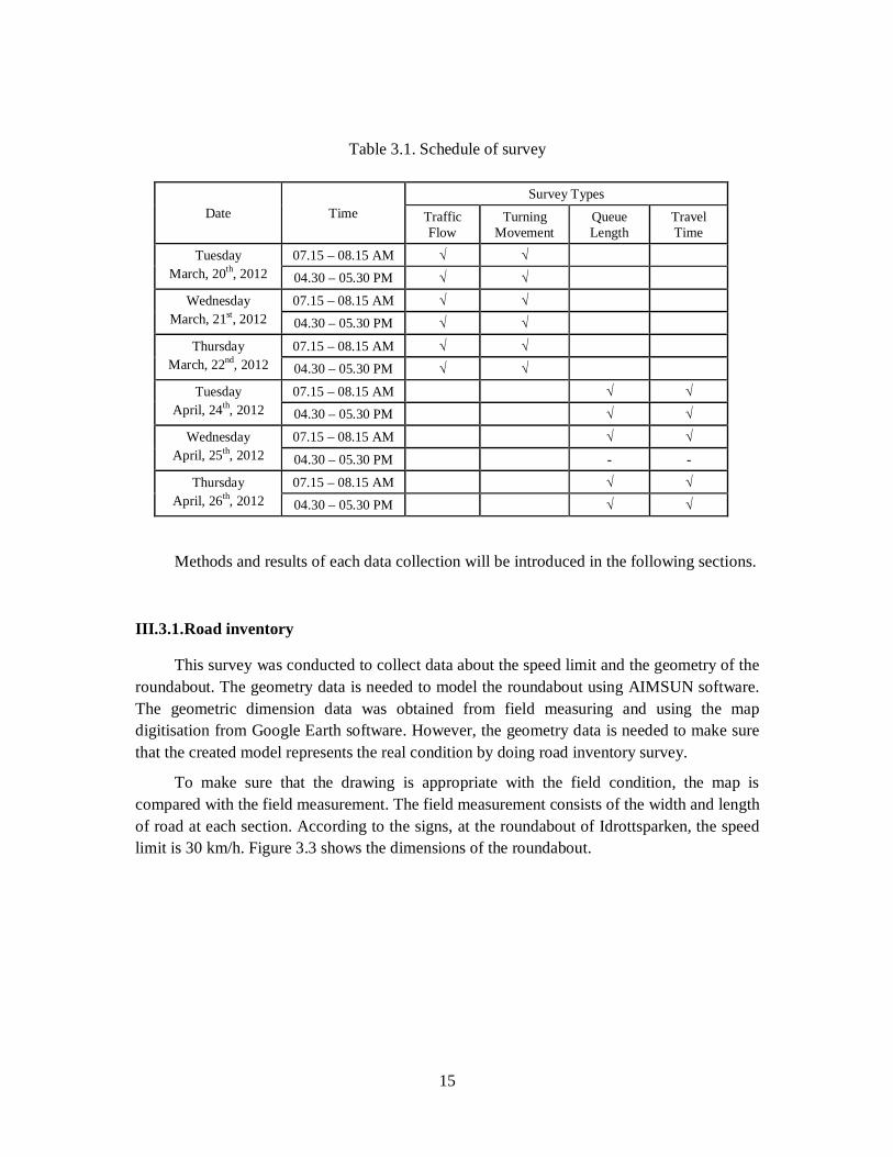
In this project, the surveys to collect the data were conducted at both of peak hours within one week. Each data set is observed in three weekdays from Tuesday until Thursday. The schedule of the survey can be seen in Table 3.1 below.

: Surveyor in North section : Surveyor in East section : Surveyor in South section : Surveyor in West section

A

B

C

D

15

Table 3.1. Schedule of survey

Date Time Survey Types

Traffic Flow

Turning Movement

Queue Length

Travel Time

Tuesday March, 20th, 2012

07.15 – 08.15 AM √ √ 04.30 – 05.30 PM √ √

Wednesday March, 21st, 2012

07.15 – 08.15 AM √ √ 04.30 – 05.30 PM √ √

Thursday March, 22nd, 2012

07.15 – 08.15 AM √ √ 04.30 – 05.30 PM √ √

Tuesday April, 24th, 2012

07.15 – 08.15 AM √ √ 04.30 – 05.30 PM √ √

Wednesday April, 25th, 2012

07.15 – 08.15 AM √ √

04.30 – 05.30 PM - -

Thursday April, 26th, 2012

07.15 – 08.15 AM √ √ 04.30 – 05.30 PM √ √

Methods and results of each data collection will be introduced in the following sections.

III.3.1. Road inventory

This survey was conducted to collect data about the speed limit and the geometry of the roundabout. The geometry data is needed to model the roundabout using AIMSUN software. The geometric dimension data was obtained from field measuring and using the map digitisation from Google Earth software. However, the geometry data is needed to make sure that the created model represents the real condition by doing road inventory survey.

To make sure that the drawing is appropriate with the field condition, the map is compared with the field measurement. The field measurement consists of the width and length of road at each section. According to the signs, at the roundabout of Idrottsparken, the speed limit is 30 km/h. Figure 3.3 shows the dimensions of the roundabout.

16

Figure 3.4. The dimension of the Idrottsparken roundabout

III.3.2. Traffic flow count

Traffic flow is the most important data which is used to construct model in AIMSUN. It includes the type of vehicle, the turning proportion and the origin-destination at a certain time of period.

In this survey, the types of vehicles have been divided into three categories: car, bus and truck. For the turning proportions, it has been divided into three directions which are: turn left, straight through and turn right. The traffic flow data was recorded at 5 minute for an hour of every survey in order to make it possible to observe changes over time. To observe the O-D flow correctly and accurately, each of surveyors stood at the corner in each section of the roundabout and keeps counting during the observation period. The surveyors could only focus on the flow coming from their directions to avoid or mitigate count error due to the heavy flow in a certain peak hour.

The results of traffic flow and turning movement counting from each direction are shown in Table 3.2 to 3.5. The results of these OD-flow observations will be used as an input of AIMSUN model. More details can be found in Appendix 2.

Table 3.2. Traffic flow count per section in morning

NORTH EAST SOUTH WEST

Car Bus Truck Car Bus Truck Car Bus Truck Car Bus Truck

Total (veh) 926 18 16 998 1 6 1265 8 8 1352 2 18

(%) 96.46 1.87 1.67 99.30 0.10 0.60 98.76 0.62 0.62 98.54 0.15 1.31

17

Table 3.3. Traffic flow count per section in afternoon

NORTH EAST SOUTH WEST

Car Bus Truck Car Bus Truck Car Bus Truck Car Bus Truck

Total (veh) 1463 15 5 1407 0 2 1073 8 1 1464 2 3

(%) 98.65 1.01 0.34 99.86 0 0.14 99.17 0.74 0.09 99.66 0.14 0.20

Table 3.4. Turning proportion per type of vehicle in morning

NORTH APPROACH

Car Bus Truck

Turn Left

Through Turn Right

Turn Left

Through Turn Right

Turn Left

Through Turn Right

Total (veh) 139 518 269 8 9 1 3 11 2 (%) 15.01 55.94 29.05 44.44 50 5.56 18.75 68.75 12.50

EAST APPROACH

Car Bus Truck

Turn Left

Through Turn Right

Turn Left

Through Turn Right

Turn Left

Through Turn Right

Total (veh) 147 640 211 0 1 0 0 5 1 (%) 14.73 64.13 21.14 0 100 0 0 83.33 16.67

SOUTH APPROACH

Car Bus Truck

Turn Left

Through Turn Right

Turn Left

Through Turn Right

Turn Left

Through Turn Right

Total (veh) 247 777 241 1 6 1 1 6 1 (%) 19.53 61.42 19.05 12.50 75 12.50 12.50 75 12.50

WEST APPROACH

Car Bus Truck

Turn Left

Through Turn Right

Turn Left

Through Turn Right

Turn Left

Through Turn Right

Total (veh) 345 864 143 2 0 0 6 10 2 (%) 25.52 63.90 10.58 100 0 0 33.33 55.56 11.11

18

Table 3.5. Turning proportion per type of vehicle in afternoon

NORTH APPROACH

Car Bus Truck

Turn Left

Through Turn Right

Turn Left

Through Turn Right

Turn Left

Through Turn Right

Total (veh) 234 913 316 2 11 2 1 4 0 (%) 15.99 62.41 21.60 13.33 73.34 13.33 20 80 0

EAST APPROACH

Car Bus Truck

Turn Left

Through Turn Right

Turn Left

Through Turn Right

Turn Left

Through Turn Right

Total (veh) 319 891 197 0 0 0 1 0 1 (%) 22.67 63.33 14 0 0 0 50 0 50

SOUTH APPROACH

Car Bus Truck

Turn Left

Through Turn Right

Turn Left

Through Turn Right

Turn Left

Through Turn Right

Total (veh) 232 580 261 0 8 0 0 1 0 (%) 21.62 54.06 24.32 0 100 0 0 100 0

WEST APPROACH

Car Bus Truck

Turn Left

Through Turn Right

Turn Left

Through Turn Right

Turn Left

Through Turn Right

Total (veh) 272 914 278 0 2 0 0 2 1 (%) 18.58 62.43 18.99 0 100 0 0 66.67 33.33

III.3.3. Queue survey

This data will be used for the calibration process. For the queue length data collection, the vehicles which were totally stopped in the queue waiting to enter the roundabout were counted by surveyors. The queue length data were recorded every 5 minutes for an hour of each survey. The observation time was in the morning peak hour between 07.15-08.15 AM and in the afternoon peak hour between 04.30-05.30 PM which is same as the travel time observation time. The maximum queue length is determined based on the longest queue in one hour period of observation. Table 3.6 and Table 3.7 show the results of queue length observation from each direction. Detailed information of each single queue length measurement result can be found in Appendix 3.

Table 3.6. Queue length in morning

QUEUE LENGTH (veh) North Approach East Approach South Approach West Approach

Max 10 15 16 5 Min 2 3 3 2

Average 3.111 5.639 6.861 2.278

19

Table 3.7. Queue length in afternoon

QUEUE LENGTH (veh) North Approach East Approach South Approach West Approach

Max 12 12 10 7 Min 3 2 2 2

Average 5.625 5.250 4.792 3.250

From tables above, it can be seen that the queue length in the morning peak hour is longer than that in the afternoon peak hour. The queue observation results show that East and South sections have the biggest maximum queue length in the morning; North and East sections have the biggest maximum queue length in the afternoon.

III.3.4. Travel time measurements

Travel time measurements are performed by fixing certain reference points in each section: 80 m in north section, 122 m in east section, 117 m in south section, and 127 m in west section. The travel time of each vehicle is measured when the vehicle enters one certain point and exits another certain point. The surveyor selects the vehicles randomly, then measures the travel time during one hour for each survey (07.15 – 08.15 AM and 04.30 – 05.30 PM) by using stopwatch. The surveyors recorded the travel time in five minutes time intervals.

The travel time samples will be taken as many as possible during one hour. The mean value of travel time obtained from the sum of measurement in one hour divided by the number of measurement in one hour. The Table 3.8 and Table 3.9 below show the mean value of travel time for each approach. More details can be found in Appendix 4.

Table 3.8. Travel time in morning

Day TRAVEL TIME (sec) North Approach East Approach South Approach West Approach

1st 16.70 22.34 24.80 17.27 2nd 17.24 22.99 23.40 16.72 3rd 15.17 23.98 42.49 17.81

Table 3.9. Travel time in afternoon

Day TRAVEL TIME (sec) North Approach East Approach South Approach West Approach

1st 21.27 20.57 19.19 19.63 2nd - - - - 3rd 29.20 19.41 21.44 21.68

As shown in tables above, it can be seen that the travel time in the North and West sections during the morning peak hour is shorter than in the afternoon peak hour. In contrary,

20

the travel time in the East and South sections during the morning peak hour is longer than in the afternoon peak hour. These results are consistent with the maximum queue observations.

.

21

IV. MODELING AND SIMULATION

IV.1. Base Model Development

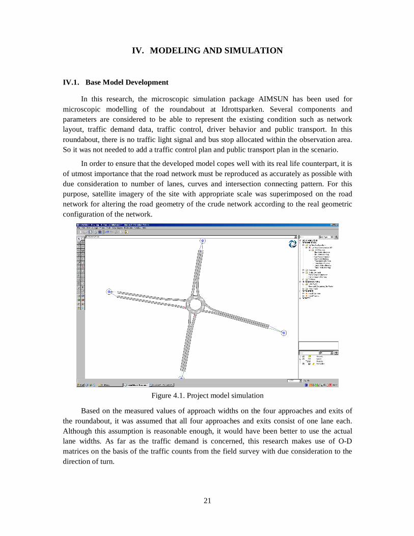
In this research, the microscopic simulation package AIMSUN has been used for microscopic modelling of the roundabout at Idrottsparken. Several components and parameters are considered to be able to represent the existing condition such as network layout, traffic demand data, traffic control, driver behavior and public transport. In this roundabout, there is no traffic light signal and bus stop allocated within the observation area. So it was not needed to add a traffic control plan and public transport plan in the scenario.

In order to ensure that the developed model copes well with its real life counterpart, it is of utmost importance that the road network must be reproduced as accurately as possible with due consideration to number of lanes, curves and intersection connecting pattern. For this purpose, satellite imagery of the site with appropriate scale was superimposed on the road network for altering the road geometry of the crude network according to the real geometric configuration of the network.

Figure 4.1. Project model simulation

Based on the measured values of approach widths on the four approaches and exits of the roundabout, it was assumed that all four approaches and exits consist of one lane each. Although this assumption is reasonable enough, it would have been better to use the actual lane widths. As far as the traffic demand is concerned, this research makes use of O-D matrices on the basis of the traffic counts from the field survey with due consideration to the direction of turn.

22

IV.2. Error Checking

Error checking proceeds divided into three basic stages: (1) software error checking; (2) input coding error checking; and (3) animation review. Input coding error checking consist of a checklist for verifying the accuracy of the coded input data such as link and code network, demand, and traveler behavior and vehicle characteristics (FHWA, 2004).

This research was conducted with AIMSUN version 6.1 standard. Software errors are tested by review of the model documentation and other material for input/output data in the software. The result indicated that there were no known problems or bugs related to the network under study and the scenarios to be simulated.

Table 4.1. Input coding error checking

Coding Error Checking North to East to South to West to

W S E N W S E N W S E N Link and code network: a. Basic network

connectivity √ √ √ √ √ √ √ √ √ √ √ √

b. Link geometry (size of roundabout, number of lanes, free-flow speed)

√ √ √ √ √ √ √ √ √ √ √ √

Demand: c. Check the identified O-

D for traffic. √ √ √ √ √ √ √ √ √ √ √ √

d. Vehicles turning movement √ √ √ √ √ √ √ √ √ √ √ √

Traveller behaviour and vehicle characteristics:

e. The default vehicle types √ √ √ √ √ √ √ √ √ √ √ √

f. vehicle mix proportions √ √ √ √ √ √ √ √ √ √ √ √

After the coding error checking have done and already correct and appropriate as described in Table 4.1, in order to visually check the errors associated with the simulation model, the model was run in the form of an animated simulation. If a rigorous scrutiny of the animation regarding vehicle types, vehicle manoeuvres and route choice shows animated results look fine based on judgment or field inspection, it can be concluded that the model is free from errors and therefore, it is acceptable to proceed with it in the subsequent steps, the calibration and validation process.

23

IV.3. Calibration Process

IV.3.1. Model parameter setting

The first step in model parameter setting began with the adjustment of the more general global parameter, such as driver reaction time and reaction time at stop. Driver reaction time and reaction time at stop are two user specified driver behaviour parameter that strongly influence the performance and capacity of the network (FHWA, 2004). Once these parameters were adjusted to produce a good fit between observed and modelled data, and then began to have little further influence on the model outputs, local model parameter were adjusted. This was a speed limit. This parameter is defined at the section level and applied locally to vehicles while they are driving along a section. The last parameter to be adjusted is maximum acceleration in vehicles attribute parameter.

IV.3.2. Optimal Parameter Value

According to the literature review, the Root Mean Square Error (RMSE) method is used to get a minimum error value between the model measurements and the field measurements of capacity. In this research, two significantly influencing parameters for the queue length and travel time are simulation time step (driver reaction time) and maximum acceleration.

To find the RMSE value, two parameters that significantly influencing the capacity of the network are used. For driver reaction time parameter, the value used is in the range 0.55 to 1.05, and for maximum acceleration parameter, the range of values used is 1 to 3. The results of RMSE minimization in the morning peak hour can be seen in Figure 4.2, Figure 4.3 and Table 4.2.

Note : Max Acceleration 1 : max = 3, mean = 3, min = 3

Max Acceleration 2 : max = 3, mean = 2.5, min = 2 Max Acceleration 3 : max = 2, mean = 1.5, min = 1 Max Acceleration 4 : max = 1, mean = 1, min = 1

Figure 4.2. Minimization of RMSE between the model output and the field measurements by using maximum queue length data in morning

0

1

2

3

4

5

0.55 0.65 0.75 0.85 0.95 1.05

Roo

t Mea

n Sq

uare

Err

or

Driver Reaction Time (sec)

Max Acceleration 1

Max Acceleration 2

Max Acceleration 3

Max Acceleration 4

24

From figure above, the result shows that by using parameters driver reaction time = 0.65 and maximum acceleration: max = 3, mean = 2.5, min = 2, the minimum RMSE value for queue length data in the morning peak hour is obtained.



Figure 4.3. Minimization of RMSE between the model output and the field measurements by using travel time data in morning

From Figure 4.3, the result shows that by using parameters driver reaction time = 0.65 and maximum acceleration max = 1, mean = 1, min = 1, the minimum RMSE value for travel time data in the morning peak hour is obtained.

Ideally, a combination of performance measures should be used for the calibration of a model. To get the optimal value of RMSE between queue length data and travel time data, the RMSE results is combined by adding the individual of results. Conversion factors will be used to equalize the unit between the queue length (in vehicle) and travel time (in second), so the RMSE values can be summed. To obtain the conversion factors, the total vehicles from field measurement is used with the assumption a single unit truck/bus is equivalent to 1.5 passenger car unit (pcu) and a truck with trailer is equivalent to 2 pcu (FHWA, 2000). According to the assumptions, the conversion factors in the morning peak hour is 1547.7/3600 = 0.430 veh/sec, while the conversion factors in the afternoon peak hour is 1828.2/3600 = 0.508 veh/sec. Then, the conversion value will be multiplied with the RMSE value of travel time. After that, the new of the RMSE of travel time can be added to the RMSE of queue length to obtain the RMSE combination between queue length and travel time.

2.5

3.5

4.5

5.5

6.5

7.5

8.5

0.55 0.65 0.75 0.85 0.95 1.05

Roo

ot M

ean

Squa

re E

rror

Driver Reaction Time (s)

Max Acceleration 1

Max Acceleration 2

Max Acceleration 3

Max Acceleration 4

25

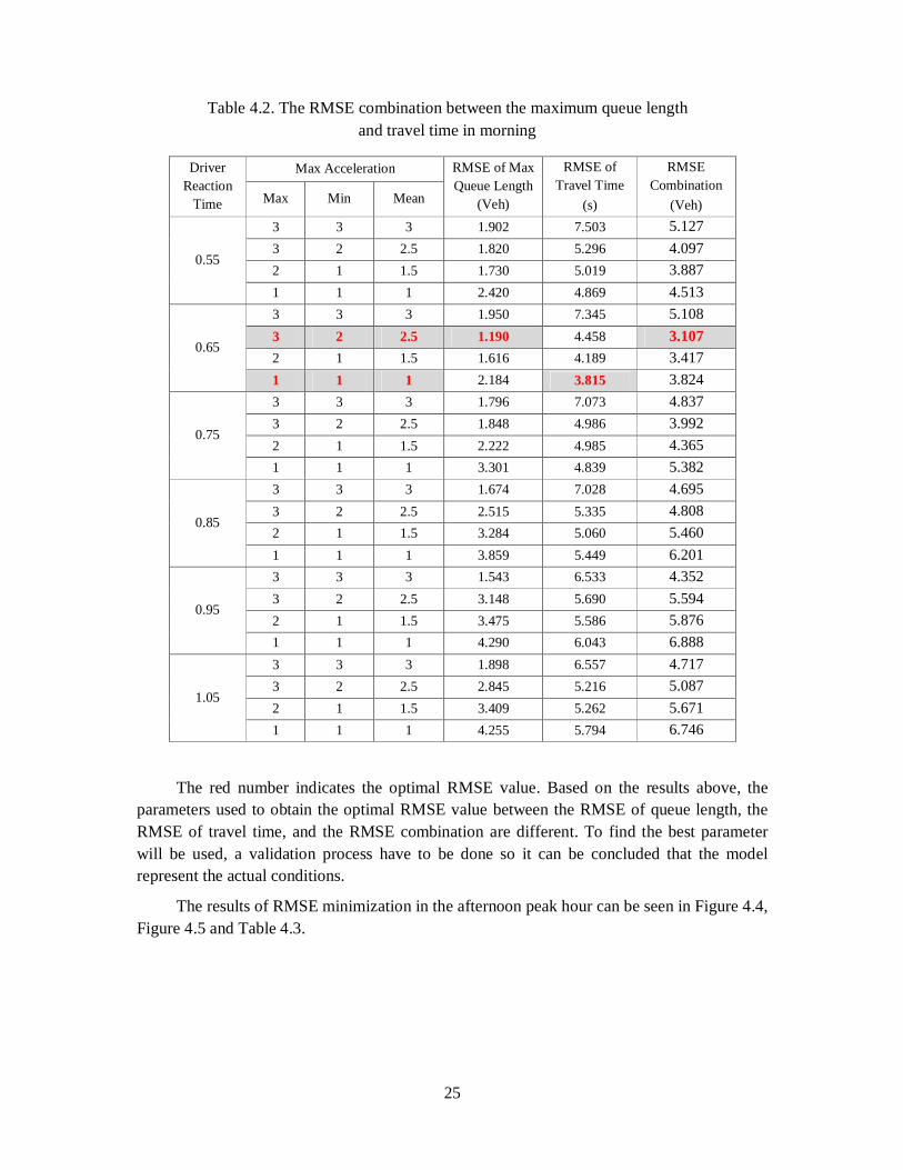
Table 4.2. The RMSE combination between the maximum queue length and travel time in morning

Driver Reaction

Time

Max Acceleration RMSE of Max Queue Length

(Veh)

RMSE of Travel Time

(s)

RMSE Combination

(Veh) Max Min Mean

0.55

3 3 3 1.902 7.503 5.127 3 2 2.5 1.820 5.296 4.097 2 1 1.5 1.730 5.019 3.887 1 1 1 2.420 4.869 4.513

0.65

3 3 3 1.950 7.345 5.108 3 2 2.5 1.190 4.458 3.107 2 1 1.5 1.616 4.189 3.417 1 1 1 2.184 3.815 3.824

0.75

3 3 3 1.796 7.073 4.837 3 2 2.5 1.848 4.986 3.992 2 1 1.5 2.222 4.985 4.365 1 1 1 3.301 4.839 5.382

0.85

3 3 3 1.674 7.028 4.695 3 2 2.5 2.515 5.335 4.808 2 1 1.5 3.284 5.060 5.460 1 1 1 3.859 5.449 6.201

0.95

3 3 3 1.543 6.533 4.352 3 2 2.5 3.148 5.690 5.594 2 1 1.5 3.475 5.586 5.876 1 1 1 4.290 6.043 6.888

1.05

3 3 3 1.898 6.557 4.717 3 2 2.5 2.845 5.216 5.087 2 1 1.5 3.409 5.262 5.671 1 1 1 4.255 5.794 6.746

The red number indicates the optimal RMSE value. Based on the results above, the parameters used to obtain the optimal RMSE value between the RMSE of queue length, the RMSE of travel time, and the RMSE combination are different. To find the best parameter will be used, a validation process have to be done so it can be concluded that the model represent the actual conditions.

The results of RMSE minimization in the afternoon peak hour can be seen in Figure 4.4, Figure 4.5 and Table 4.3.

26



Figure 4.4. Minimization of RMSE between the model output and the field measurements by using maximum queue length data in afternoon



Figure 4.5. Minimization of RMSE between the model output and the field measurements by using travel time data in afternoon

From Figure 4.4 and 4.5, the result shows that by using parameters Driver Reaction Time= 0.55 and maximum acceleration Max = 3, Mean = 2.5, Min = 2, the RMSE minimization value for both of queue length data and travel time data in the afternoon peak hour is obtained.

0

1

2

3

4

5

0.55 0.65 0.75 0.85 0.95 1.05

Roo

t Mea

n Sq

uare

Err

or

Driver Reaction Time (sec)

Max Acceleration 1

Max Acceleration 2

Max Acceleration 3

Max Acceleration 4

2.5

3.5

4.5

5.5

6.5

7.5

8.5

0.55 0.65 0.75 0.85 0.95 1.05

Roo

t Mea

n Sq

uare

Err

or

Driver Reaction Time (s)

Max Acceleration 1

Max Acceleration 2

Max Acceleration 3

Max Acceleration 4

27

Table 4.3. The RMSE combination between the maximum queue length and travel time in afternoon

Driver Reaction

Time

Max Acceleration RMSE of Max Queue Length

(Veh)

RMSE of Travel Time

(s)

RMSE Combination

(Veh) Max Min Mean

0.55

3 3 3 1.695 11.533 7.552 3 2 2.5 1.026 8.335 5.259 2 1 1.5 1.299 9.172 5.957 1 1 1 1.649 10.110 6.783

0.65

3 3 3 2.178 11.042 7.786 3 2 2.5 1.623 9.112 6.250 2 1 1.5 2.082 9.737 7.026 1 1 1 2.715 10.765 8.182

0.75

3 3 3 2.151 10.645 7.557 3 2 2.5 2.166 10.289 7.392 2 1 1.5 2.885 10.825 8.382 1 1 1 3.473 11.793 9.462

0.85

3 3 3 3.016 10.167 8.179 3 2 2.5 2.569 11.598 8.459 2 1 1.5 3.191 11.258 8.909 1 1 1 4.113 13.531 10.984

0.95

3 3 3 4.523 9.627 9.412 3 2 2.5 3.314 12.529 9.676 2 1 1.5 4.174 12.701 10.624 1 1 1 4.665 14.041 11.796

1.05

3 3 3 2.795 10.418 8.086 3 2 2.5 3.720 13.367 10.508 2 1 1.5 4.185 14.171 11.381 1 1 1 4.616 14.676 12.069

Based on the results above, the parameters used to obtain the optimal RMSE value between the RMSE of queue length, the RMSE of travel time, and the RMSE combination are the same parameters. Before it can be concluded that the model represent the actual conditions, a validation process have to be done. The parameters that were calibrated are shown in Table 4.4 below.

28

Table 4.4. Calibrated model parameter

No Parameter Adjustment Default Value Calibrated Value

Morning Afternoon

1. Global Parameter

Simulation time step (driver reaction time) 0.75 0.65 0.55

Reaction time at stop 1.35 1.1 1.1

2. Local Section Parameter

Speed limit (arterial) 50 30

3. Vehicle Parameter

Maximum Acceleration

- Max 3.4 3 1 3

- Mean 3 2.5 1 2.5

- Min 2.6 2 1 2

Minimum Distance Vehicle

- Max 1.5 2 2

- Mean 1 1.5 1.5

- Min 0.5 1 1

IV.4. Validation Process

In this process, we used the travel time data as comparison to the output from modeling. T-test method is used in the validation process to check whether the simulation model is good enough to satisfy any other measured traffic performance. For validation procedure, the equations used are equation (3) – (9) as expressed in section II.4. The result of the validation of the mean travel time is shown in the Table 4.5 and 4.6 below.

Table 4.5. Result for validation model in morning (driver reaction time = 0.65 and max acceleration: max = 3, mean = 2.5, min = 2)

North Section East Section South Section West Section The Measured Data

풏풙 12 12 12 12 풙 16.369 23.108 30.231 17.268 푺풙 2.747 6.866 4.939 2.970

The Calibrated Model 풏풚 12 12 12 12 풚 14.187 23.633 21.755 18.887 푺풚 0.223 1.399 0.585 0.749 푺풑 1.948 4.937 9.560 2.154

T-statistic 2.744 -0.261 2.172 -1.841 풕풏풙 풏풚 ퟐ(∝ ퟐ) 2.074

Validity* No Yes No Yes * Validity : Yes = similar, No = unsimilar

29

Table 4.6. Result for validation model in morning (driver reaction time = 0.65 and max acceleration: max = 1, mean = 1, min = 1)


풏풙 12 12 12 12 풙 16.369 23.108 30.231 17.268 푺풙 2.747 6.866 4.939 2.970



Validity* Yes Yes Yes Yes * Validity : Yes = similar, No = unsimilar

According to the assumption: if |푇| < 푡 (훼 2), then it is considered as 휇 =휇 , the hypothesis cannot be rejected and validation is successful. In this case, all the T-values are satisfied. It means that the output of simulation data is similar with the observed data.

From Table 4.5 and 4.6, by using parameter of driver reaction time = 0.65 and max acceleration max = 1, mean = 1, min = 1, the model satisfies with all sections and it means the model represent the actual conditions in morning peak hour. Whereas when using parameter of driver reaction time = 0.65 and max acceleration: max = 3, mean = 2.5, min = 2, the model only satisfies on East and West sections.

By using t-test method, the travel time data of the validation model have no significance differences compared to the measured data since the T value is in range -2.074 ≤ T ≤ 2.074. The travel time in the output of AIMSUN is checked to ensure that the model has the same travel time as the input does.

Figure 4.6. Measured travel time versus validated travel time on

North section in morning

10

13

16

19

22

0 5 10 15 20 25 30 35 40 45 50 55 60

Trav

el T

ime

(s)

Time (min)

Measured Model

Validated Model

30

Figure 4.7. Measured travel time versus validated travel time on East section in morning

Figure 4.8. Measured travel time versus validated travel time on South section in morning

Figure 4.9. Measured travel time versus validated travel time on West

section in morning

10

15

20

25

30

35

40

0 5 10 15 20 25 30 35 40 45 50 55 60

Trav

el T

ime

(s)

Time (min)

Measured Model

Validated Model

10

20

30

40

50

60

0 5 10 15 20 25 30 35 40 45 50 55 60

Trav

el T

ime

(s)

Time (min)

Measured Model

Validated Model

10

13

16

19

22

25

28

0 5 10 15 20 25 30 35 40 45 50 55 60

Trav

el T

ime

(s)

Time (min)

Measured Model

Validated Model

31

From Figures 4.6 to 4.9, it can be concluded that the travel time of the model is similar with the observed data. Although in AIMSUN output the deviation between the highest value and the lowest value is very small compared to observed data of travel time.

Table 4.7. Final result for validation model in afternoon (driver reaction time = 0.55 and max acceleration: max = 3, mean = 2.5, min = 2)


풏풙 12 12 12 12 풙 25.240 19.989 20.312 20.655 푺풙 4.748 4.360 2.792 1.843



Validity* Yes Yes Yes Yes * Validity : Yes = similar, No = unsimilar

From Table 4.7, by using parameter of driver reaction time = 0.55 and max acceleration: max = 3, mean = 2.5, min = 2, the model satisfies with all sections and it means the model represent the actual conditions in afternoon peak hour. To ensure that the model has the same travel time as the input does, the travel time in the output of AIMSUN is compared with the travel time in observed data.

Figure 4.10. Measured travel time versus validated travel time on North section in afternoon

10

15

20

25

30

35

0 5 10 15 20 25 30 35 40 45 50 55 60

Trav

el T

ime

(s)

Time (min)

Measured Model

Validated Model

32

Figure 4.11. Measured travel time versus validated travel time on East section in afternoon


South section in afternoon


West section in afternoon

10

15

20

25

30

35

0 5 10 15 20 25 30 35 40 45 50 55 60

Trav

el T

ime

(s)

Time (min)

Measured Model

Validated Model

10

13

16

19

22

25

28

0 5 10 15 20 25 30 35 40 45 50 55 60

Trav

el T

ime

(s)

Time (min)

Measured Model

Validated Model

10

15

20

25

30

35

40

0 5 10 15 20 25 30 35 40 45 50 55 60

Trav

el T

ime

(s)

Time (min)

Measured Model

Validated Model

33

Similar with output in morning peak hour, it can be concluded that the travel time of the model is similar with the travel time in the observed data. After the steps of calibration and validation which result the conclusion that the model is acceptable and appropriate with the field condition, then the model is ready to be analyzed for further steps.

35

V. ALTERNATIVE SCENARIOS

The proposed three scenarios have been developed in order to improve the performance of the roundabout. The first scenario is an addition of free right turn (exit side lane) on two sections (north and east section), the second scenario is an addition of free right turn on east and south section, and the third scenario is addition of one lane on the roundabout.

The effectiveness of these approaches would be observed in terms of queue length and travel time on these approaches. The success indicator is obtained from the reduce queue length and travel time. If the queue length and the travel time in sections are reduced, it means the proposed scenarios successfully improve the performance of the roundabout and thus, the proposed scenario is acceptable.

V.1. Alternative Scenario 1: Free right turn implementation (on North and East

sections)

Based on the visual observation of the performance of the roundabout, it was observed that there is build-up of queue on the North and East approaches. According to the collected data, the percentage of cars turning right in the morning peak hour are 29.05%, 21.14%, 19.05%, and 10.58% for North, East, South, and West sections respectively. In afternoon peak hour, the percentages of cars turning right are 21.60%, 14%, 24.32%, and 18.99% for North, East, South, and West sections. In order to reduce the queue entering the roundabout, it was decided to add one free right turn to prevent the cars taking the right turn of entering the roundabout.

According to the right turn percentage mention above, the North, East and South sections have the highest turn proportions. In terms of the possibility of implementation, since there is a building in the North and South sections, making free right turning in these sections is not easy. By considering the nearest signalized intersection on the North section with the distance from the roundabout less than 100 m, which it gives a direct effect to the length queue in the North section, it was decided to add one free right turn in this section. Therefore, the first alternative scenario in this project is making free right turning in the North and East sections. This alternative is motivated by reducing the queue length in the North and East sections.

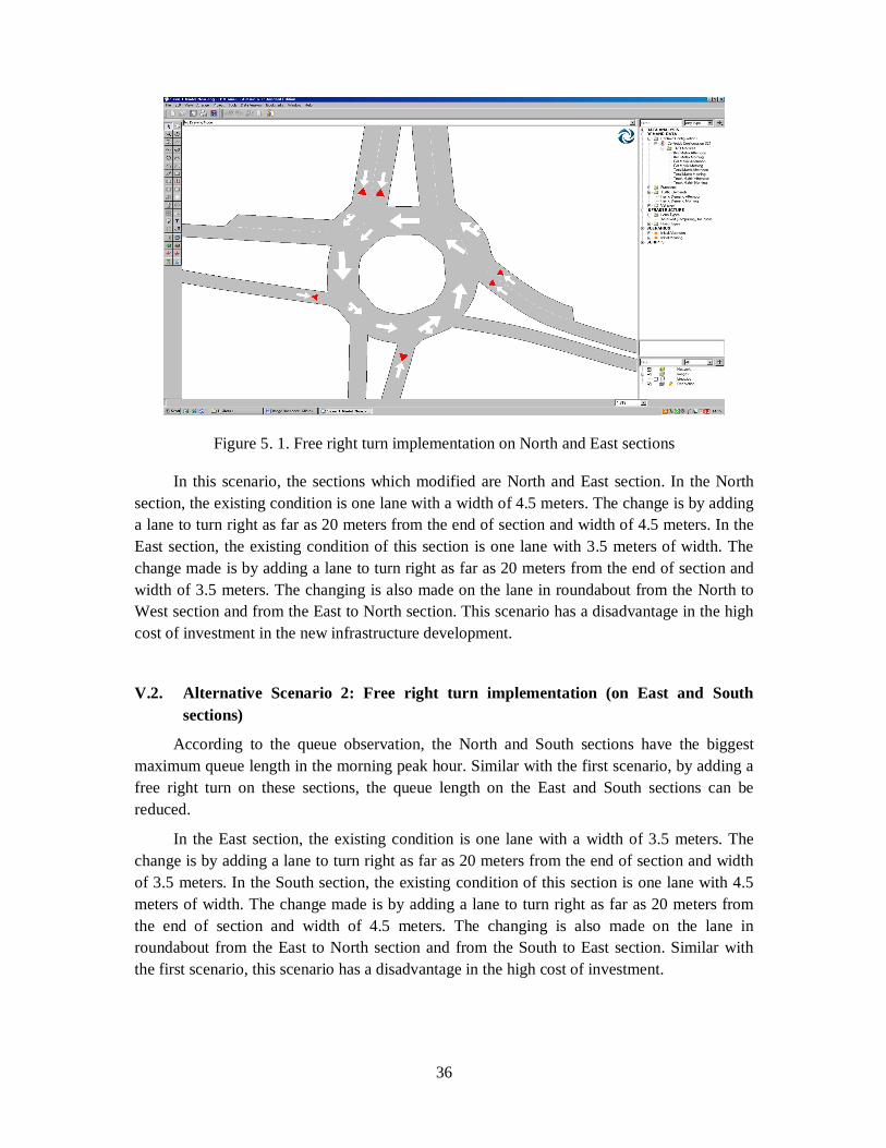
36

Figure 5. 1. Free right turn implementation on North and East sections

In this scenario, the sections which modified are North and East section. In the North section, the existing condition is one lane with a width of 4.5 meters. The change is by adding a lane to turn right as far as 20 meters from the end of section and width of 4.5 meters. In the East section, the existing condition of this section is one lane with 3.5 meters of width. The change made is by adding a lane to turn right as far as 20 meters from the end of section and width of 3.5 meters. The changing is also made on the lane in roundabout from the North to West section and from the East to North section. This scenario has a disadvantage in the high cost of investment in the new infrastructure development.

V.2. Alternative Scenario 2: Free right turn implementation (on East and South sections)

According to the queue observation, the North and South sections have the biggest maximum queue length in the morning peak hour. Similar with the first scenario, by adding a free right turn on these sections, the queue length on the East and South sections can be reduced.

In the East section, the existing condition is one lane with a width of 3.5 meters. The change is by adding a lane to turn right as far as 20 meters from the end of section and width of 3.5 meters. In the South section, the existing condition of this section is one lane with 4.5 meters of width. The change made is by adding a lane to turn right as far as 20 meters from the end of section and width of 4.5 meters. The changing is also made on the lane in roundabout from the East to North section and from the South to East section. Similar with the first scenario, this scenario has a disadvantage in the high cost of investment.

37

Figure 5.2. Free right turn implementation on East and South sections

V.3. Alternative Scenario 3: Addition of lane in roundabout

The third alternative in this project is an addition of one lane in the Idrottsparken roundabout. This alternative is motivated to increase the capacity of roundabout and to reduce the queue entering the roundabout. For double lane roundabout the minimum inscribed circle diameter based upon design vehicle and turning movements is 110 ft (33.5 m) for through direction and 125 ft (38 m) for left turn or U-turn (KYTC, 2009).

The existing condition of this roundabout is one lane with a width of 8 m. The change made is by adding one lane into two lanes with 10 meters of width for each lane. The land use taken from the outside roundabout area. The total of inscribed diameter will be 38 m. Similar to the first scenario, the disadvantages in conducting this scenario is the high cost investment. The new lane will need to cut the physical building surrounding the roundabout. The change of geometric layout is illustrated in Figure 5.3.

38

Figure 5.3. Addition of lane in roundabout

39

VI. RESULT AND ANALYSIS

VI.1. Scenario 1

By implementing the first scenario and comparing it to the validated model, the result of the queue length and travel time in the morning peak hour as expressed in the Figure 6.1, Figure 6.2 and Table 6.1.

Figure 6.1. Mean of maximum queue length between scenario 1 and the validated model in morning

Figure 6.2. Mean of travel time between scenario 1 and the validated model in morning

0.000

1.000

2.000

3.000

4.000

5.000

6.000

North East South WestValidated Model 2.992 4.225 5.092 3.000Scenario 1 1.917 3.083 5.833 3.167

Que

ue L

engt

h (v

eh)

0.000

5.000

10.000

15.000

20.000

25.000

30.000


Trav

el T

ime

(sec

)

40

Table 6.1. Comparison of the mean of maximum queue length and travel time between scenario 1 and the validated model in morning

Result

North Section East Section South Section West Section Queue Length (veh)

Travel Time (sec)

Queue Length (veh)

Travel Time (sec)

Queue Length (veh)

Travel Time (sec)

Queue Length (veh)

Travel Time (sec)

Validated Model 2.992 15.798 4.225 26.958 5.092 24.138 3.000 19.705

Scenario 1 1.917 13.987 3.083 18.963 5.833 26.250 3.167 21.273 Comparison (%) 35.93 11.47 27.02 29.66 -14.57 -8.75 -5.56 -7.96

As shown in Figure 6.1, Figure 6.2 and Table 6.1, the maximum queue length and travel time in the morning peak hour is decreased in the North and East sections compared to the validated model. In contrary, the South and West sections show that the queue length have increase of 14.57% and 5.56% , while the travel time have increased of 8.75% and 7.96% compared to the validated model. In the morning peak hour, the high percentage of decrease in queue length occurs at East section and for travel time occurs at North section which decreases by 35.93% and 29.66%.

To know the significance of the reduction, the result of the scenario 1 is tested by using the t-test method. In the hypothesis test, the 퐻 will be rejected if 푇 < −푇 or 푇 > 푇 . It indicates that the data of the simulation is invalid or there is a significance differences between the simulation data and measured data. The results of the t-test can be seen in the Table 6.2 below.

Table 6.2. The mean of maximum queue length and travel time t-test between scenario 1 and the validated model in morning

North Section East Section South Section West Section

Queue Length (veh)

Travel Time (sec)

Queue Length (veh)

Travel Time (sec)

Queue Length (veh)

Travel Time (sec)

Queue Length (veh)

Travel Time (sec)

Validated Model 풏풙 12 12 12 12 풙 2.992 15.798 4.225 26.958 5.092 24.138 3.000 19.705 푺풙 0.300 0.678 0.160 1.002 0.801 2.532 0.585 3.136

Scenario 1 풏풚 12 12 12 12 풚 1.917 13.987 3.083 18.963 5.833 26.250 3.167 21.273 푺풚 0.669 1.762 0.793 0.918 0.389 4.374 0.718 1.721 푺풑 0.518 1.311 0.537 0.941 0.627 2.176 0.552 2.486

T-statistic 5.088 3.384 5.204 20.816 -2.896 -1.562 -0.740 -1.545 풕풏풙 풏풚 ퟐ(∝ ퟐ) 2.074

Analysis Result

Significant Decrease


Significant/Insignificant Increase

Insignificant Increase

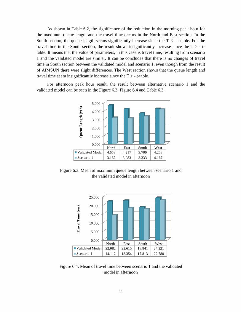
41

As shown in Table 6.2, the significance of the reduction in the morning peak hour for the maximum queue length and the travel time occurs in the North and East section. In the South section, the queue length seems significantly increase since the T < - t-table. For the travel time in the South section, the result shows insignificantly increase since the T > - t-table. It means that the value of parameters, in this case is travel time, resulting from scenario 1 and the validated model are similar. It can be concludes that there is no changes of travel time in South section between the validated model and scenario 1, even though from the result of AIMSUN there were slight differences. The West section shows that the queue length and travel time seem insignificantly increase since the T > - t-table.

For afternoon peak hour result, the result between alternative scenario 1 and the validated model can be seen in the Figure 6.3, Figure 6.4 and Table 6.3.

Figure 6.3. Mean of maximum queue length between scenario 1 and the validated model in afternoon

Figure 6.4. Mean of travel time between scenario 1 and the validated model in afternoon

0.000

1.000

2.000

3.000

4.000

5.000


Que

ue L

engt

h (v

eh)

0.000

5.000

10.000

15.000

20.000

25.000


Trav

el T

ime

(sec

)

42

Table 6.3. Comparison of the mean of maximum queue length and travel time between scenario 1 and the validated model in afternoon

Result


Travel Time (sec)

Queue Length (veh)

Travel Time (sec)

Queue Length (veh)

Travel Time (sec)

Queue Length (veh)

Travel Time (sec)

Validated Model 4.658 22.082 4.217 22.615 3.700 18.841 4.258 24.221

Scenario 1 3.167 14.112 3.083 18.354 3.333 17.813 4.167 22.780 Comparison (%) 32.02 36.09 26.88 18.84 9.91 5.45 2.15 5.95

Based on Figure 6.3, Figure 6.4 and Table 6.3, the maximum queue length and travel time in afternoon peak hour is decreased in all sections compared to the existing model. The high percentage of decrease in queue length and travel time occurs at North section which decreases by 32.02% and 36.09%. The results of the t-test can be seen in the Table 6.4 below.

Table 6.4. The mean of maximum queue length and travel time t-test between scenario 1 and the validated model in afternoon


Queue Length (veh)

Travel Time (sec)

Queue Length (veh)

Travel Time (sec)

Queue Length (veh)

Travel Time (sec)

Queue Length (veh)

Travel Time (sec)



T-statistic 4.453 9.923 3.737 14.377 1.033 1.670 0.296 0.762 풕풏풙 풏풚 ퟐ(∝ ퟐ) 2.074

Analysis Result Significant Decrease


Insignificant Decrease


As shown in Table 6.4, the significance of the reduction in the afternoon peak hour for the maximum queue length and the travel time occurs in North and East section. In the South and West sections, the queue length and travel time seem insignificantly reduce since the T < t-table. It means that the values of parameters, in this case are queue length and travel time, resulting from scenario 1 and validated model are similar. It can be concludes that in afternoon peak hour there is no changes of queue length and travel time in the South and West sections between the validated model and scenario 1.

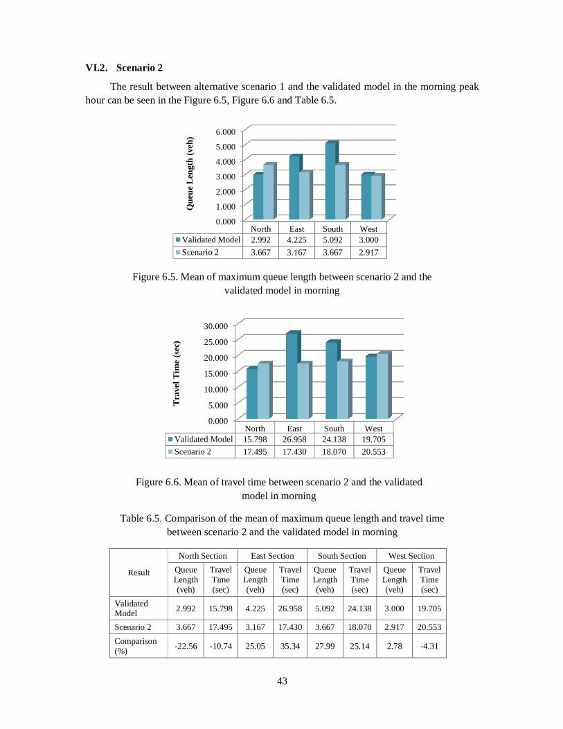
43

VI.2. Scenario 2

The result between alternative scenario 1 and the validated model in the morning peak hour can be seen in the Figure 6.5, Figure 6.6 and Table 6.5.

Figure 6.5. Mean of maximum queue length between scenario 2 and the

validated model in morning


Table 6.5. Comparison of the mean of maximum queue length and travel time between scenario 2 and the validated model in morning

Result


Travel Time (sec)

Queue Length (veh)

Travel Time (sec)

Queue Length (veh)

Travel Time (sec)

Queue Length (veh)

Travel Time (sec)

Validated Model 2.992 15.798 4.225 26.958 5.092 24.138 3.000 19.705

Scenario 2 3.667 17.495 3.167 17.430 3.667 18.070 2.917 20.553 Comparison (%) -22.56 -10.74 25.05 35.34 27.99 25.14 2.78 -4.31

0.000

1.000

2.000

3.000

4.000

5.000

6.000


Que

ue L

engt

h (v

eh)

0.000

5.000

10.000

15.000

20.000

25.000

30.000


Trav

el T

ime

(sec

)

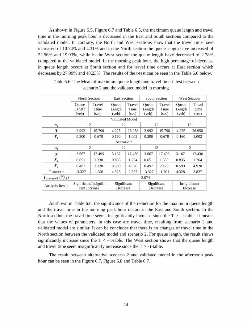
44

As shown in Figure 6.5, Figure 6.7 and Table 6.5, the maximum queue length and travel time in the morning peak hour is decreased in the East and South sections compared to the validated model. In contrary, the North and West sections show that the travel time have increased of 10.74% and 4.31% and in the North section the queue length have increased of 22.56% and 19.03%, while in the West section the queue length have decreased of 2.78% compared to the validated model. In the morning peak hour, the high percentage of decrease in queue length occurs at South section and for travel time occurs at East section which decreases by 27.99% and 40.23%. The results of the t-test can be seen in the Table 6.6 below.

Table 6.6. The Mean of maximum queue length and travel time t- test between scenario 2 and the validated model in morning


Queue Length (veh)

Travel Time (sec)

Queue Length (veh)

Travel Time (sec)

Queue Length (veh)

Travel Time (sec)

Queue Length (veh)

Travel Time (sec)



T-statistic -3.327 -1.301 4.328 2.827 -3.327 -1.301 4.328 2.827 풕풏풙 풏풚 ퟐ(∝ ퟐ) 2.074

Analysis Result Significant/Insignificant Increase




As shown in Table 6.6, the significance of the reduction for the maximum queue length and the travel time in the morning peak hour occurs in the East and South section. In the North section, the travel time seems insignificantly increase since the T > - t-table. It means that the values of parameters, in this case are travel time, resulting from scenario 2 and validated model are similar. It can be concludes that there is no changes of travel time in the North section between the validated model and scenario 2. For queue length, the result shows significantly increase since the T < - t-table. The West section shows that the queue length and travel time seem insignificantly increase since the T > - t-table.

The result between alternative scenario 2 and validated model in the afternoon peak hour can be seen in the Figure 6.7, Figure 6.8 and Table 6.7.

45



Table 6.7. Comparison of the mean of maximum queue length and travel time between scenario 2 and the validated model in afternoon

Result


Travel Time (sec)

Queue Length (veh)

Travel Time (sec)

Queue Length (veh)

Travel Time (sec)

Queue Length (veh)

Travel Time (sec)

Validated Model 4.658 22.082 4.217 22.615 3.700 18.841 4.258 24.221

Scenario 2 4.417 18.333 3.833 15.722 2.833 16.832 4.000 23.454 Comparison (%) 5.19 16.98 9.09 30.48 23.42 10.66 6.07 3.17

0.000

1.000

2.000

3.000

4.000

5.000


Que

ue L

engt

h (v

eh)

0.000

5.000

10.000

15.000

20.000

25.000


Trav

el T

ime

(sec

)

46

From figures and table above, the maximum queue length and travel time in the afternoon peak hour is decreased in all sections compared to the validated model. In the afternoon peak hour, the high percentage of decrease in queue length occurs at South section and travel time occurs at East section which decreases by 23.42% and 30.48%. The results of the t-test can be seen in the Table 6.8 below.

Table 6.8. The Mean of maximum queue length and travel time t-test between scenario 2 and the validated model in afternoon


Queue Length (veh)

Travel Time (sec)

Queue Length (veh)

Travel Time (sec)

Queue Length (veh)

Travel Time (sec)

Queue Length (veh)

Travel Time (sec)



T-statistic 0.859 4.047 1.170 22.694 2.133 3.565 0.734 0.428 풕풏풙 풏풚 ퟐ(∝ ퟐ) 2.074

Analysis Result Insigficant/ Significant Decrease

Insignificant/ Significant Decrease



As shown in Table 6.8, the significance of the reduction for the maximum queue length and the travel time in the afternoon peak hour occurs in the South section. In the North and East sections, the queue length seems insignificantly reduce since the T < t-table, while for the travel time the result shows significantly reduce since the T > t-table. It means that the value of parameters, in this case is queue length, resulting from scenario 2 and validated model are similar. It can be concludes that there is no changes of queue length in the North and East sections between the validated model and scenario 2. The West section shows that the queue length and the travel time seem insignificantly decrease since the T < t-table.

VI.3. Scenario 3

The result between alternative scenario 3 and the validated model in the morning peak hour can be seen in the Figure 6.9, Figure 6.10 and Table 6.9.

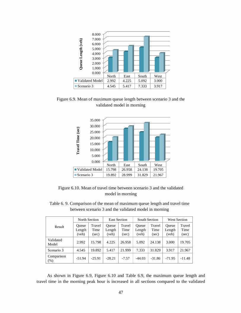
47

Figure 6.9. Mean of maximum queue length between scenario 3 and the validated model in morning


Table 6. 9. Comparison of the mean of maximum queue length and travel time between scenario 3 and the validated model in morning

Result


Travel Time (sec)

Queue Length (veh)

Travel Time (sec)

Queue Length (veh)

Travel Time (sec)

Queue Length (veh)

Travel Time (sec)

Validated Model 2.992 15.798 4.225 26.958 5.092 24.138 3.000 19.705

Scenario 3 4.545 19.892 5.417 21.999 7.333 31.829 3.917 21.967 Comparison (%) -51.94 -25.91 -28.21 -7.57 -44.03 -31.86 -71.95 -11.48

As shown in Figure 6.9, Figure 6.10 and Table 6.9, the maximum queue length and travel time in the morning peak hour is increased in all sections compared to the validated

0.0001.0002.0003.0004.0005.0006.0007.0008.000


Que

ue L

engt

h (v

eh)

0.0005.000

10.00015.00020.00025.00030.00035.000


Trav

el T

ime

(sec

)

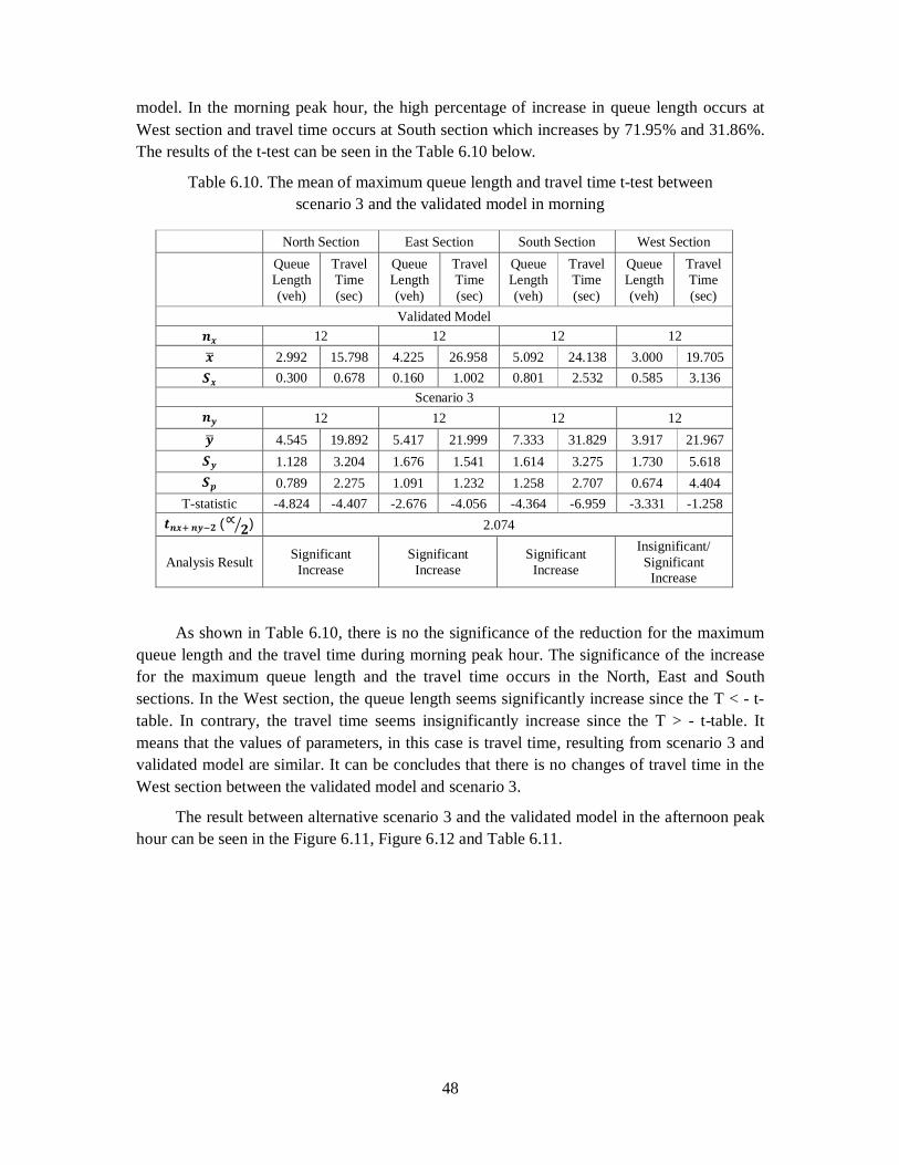
48

model. In the morning peak hour, the high percentage of increase in queue length occurs at West section and travel time occurs at South section which increases by 71.95% and 31.86%. The results of the t-test can be seen in the Table 6.10 below.

Table 6.10. The mean of maximum queue length and travel time t-test between scenario 3 and the validated model in morning


Queue Length (veh)

Travel Time (sec)

Queue Length (veh)

Travel Time (sec)

Queue Length (veh)

Travel Time (sec)

Queue Length (veh)

Travel Time (sec)



T-statistic -4.824 -4.407 -2.676 -4.056 -4.364 -6.959 -3.331 -1.258 풕풏풙 풏풚 ퟐ(∝ ퟐ) 2.074

Analysis Result Significant Increase

Significant Increase


Insignificant/ Significant

Increase

As shown in Table 6.10, there is no the significance of the reduction for the maximum queue length and the travel time during morning peak hour. The significance of the increase for the maximum queue length and the travel time occurs in the North, East and South sections. In the West section, the queue length seems significantly increase since the T < - t-table. In contrary, the travel time seems insignificantly increase since the T > - t-table. It means that the values of parameters, in this case is travel time, resulting from scenario 3 and validated model are similar. It can be concludes that there is no changes of travel time in the West section between the validated model and scenario 3.

The result between alternative scenario 3 and the validated model in the afternoon peak hour can be seen in the Figure 6.11, Figure 6.12 and Table 6.11.

49



Table 6.11. Comparison of mean of queue length and travel time between scenario 3 and the validated model in afternoon

Result


Travel Time (sec)

Queue Length (veh)

Travel Time (sec)

Queue Length (veh)

Travel Time (sec)

Queue Length (veh)

Travel Time (sec)

Validated Model 4.658 22.082 4.217 22.615 3.700 18.841 4.258 24.221

Scenario 3 7.500 29.432 5.333 23.998 6.833 25.432 5.167 26.053 Comparison (%) -61.00 -33.29 -26.48 -6.11 -84.68 -34.98 -21.33 -7.57

0.0001.0002.0003.0004.0005.0006.0007.0008.000


Que

ue L

engt

h (v

eh)

0.000

5.000

10.000

15.000

20.000

25.000

30.000


Trav

el T

ime

(sec

)

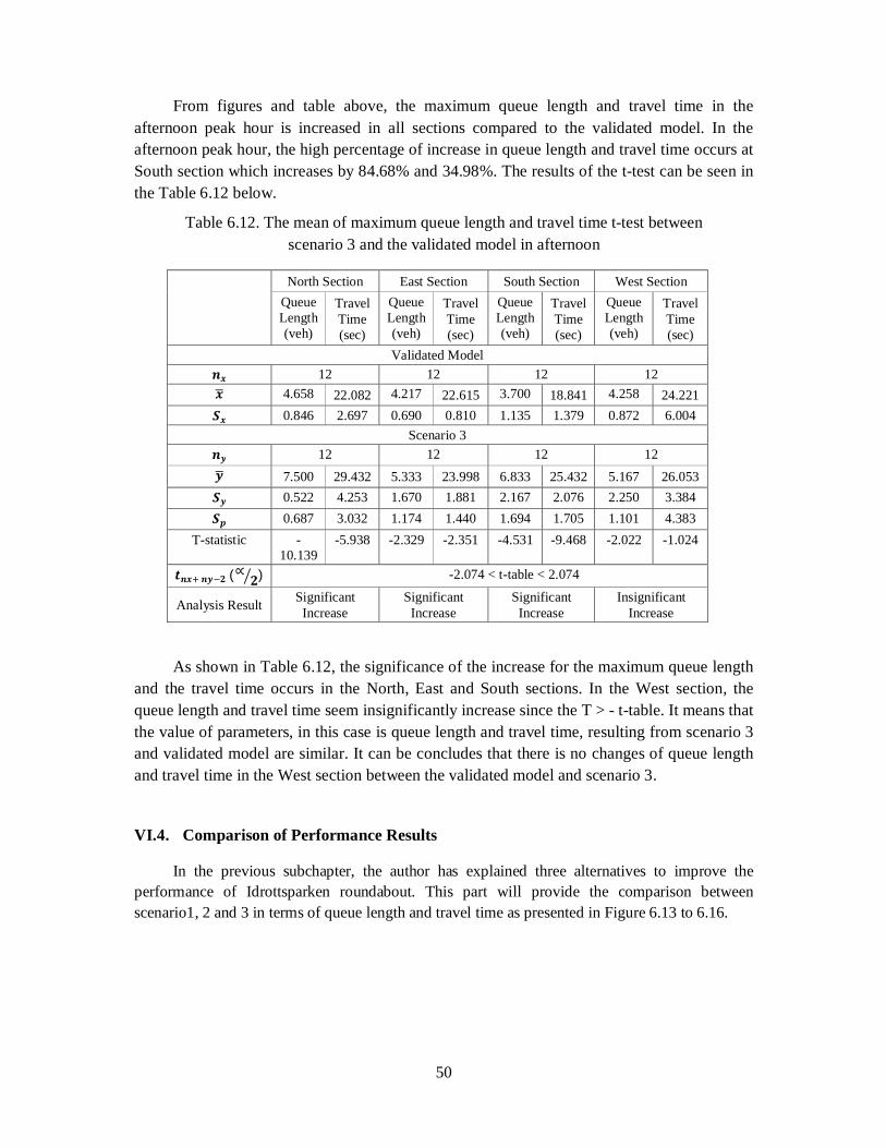
50

From figures and table above, the maximum queue length and travel time in the afternoon peak hour is increased in all sections compared to the validated model. In the afternoon peak hour, the high percentage of increase in queue length and travel time occurs at South section which increases by 84.68% and 34.98%. The results of the t-test can be seen in the Table 6.12 below.

Table 6.12. The mean of maximum queue length and travel time t-test between scenario 3 and the validated model in afternoon

North Section East Section South Section West Section Queue

Length (veh)

Travel Time (sec)

Queue Length (veh)

Travel Time (sec)

Queue Length (veh)

Travel Time (sec)

Queue Length (veh)

Travel Time (sec)



T-statistic -10.139

-5.938 -2.329 -2.351 -4.531 -9.468 -2.022 -1.024

풕풏풙 풏풚 ퟐ(∝ ퟐ) -2.074 < t-table < 2.074

Analysis Result Significant Increase




As shown in Table 6.12, the significance of the increase for the maximum queue length and the travel time occurs in the North, East and South sections. In the West section, the queue length and travel time seem insignificantly increase since the T > - t-table. It means that the value of parameters, in this case is queue length and travel time, resulting from scenario 3 and validated model are similar. It can be concludes that there is no changes of queue length and travel time in the West section between the validated model and scenario 3.

VI.4. Comparison of Performance Results

In the previous subchapter, the author has explained three alternatives to improve the performance of Idrottsparken roundabout. This part will provide the comparison between scenario1, 2 and 3 in terms of queue length and travel time as presented in Figure 6.13 to 6.16.

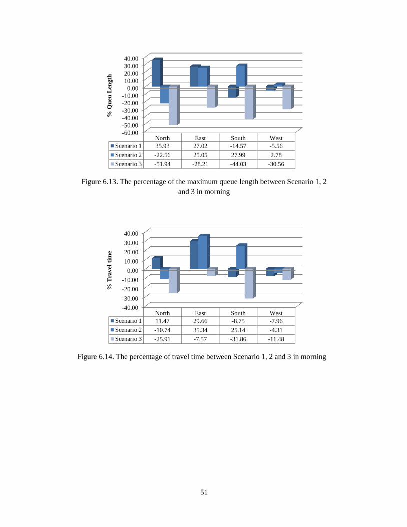
51

Figure 6.13. The percentage of the maximum queue length between Scenario 1, 2

and 3 in morning

Figure 6.14. The percentage of travel time between Scenario 1, 2 and 3 in morning

-60.00-50.00-40.00-30.00-20.00-10.00

0.0010.0020.0030.0040.00

North East South WestScenario 1 35.93 27.02 -14.57 -5.56Scenario 2 -22.56 25.05 27.99 2.78Scenario 3 -51.94 -28.21 -44.03 -30.56

% Q

ueu

Leng

th

-40.00-30.00-20.00-10.00

0.0010.0020.0030.0040.00

North East South WestScenario 1 11.47 29.66 -8.75 -7.96Scenario 2 -10.74 35.34 25.14 -4.31Scenario 3 -25.91 -7.57 -31.86 -11.48

% T

rave

l tim

e

52


and 3 in afternoon


and 3 in afternoon

As shown in figures above, in the morning peak hour, the first scenario shows the highest percentage of decrease in queue length occurs in the North section by 35.93%. For travel time, the second scenario shows the highest percentage of decrease occurs in the East section by 35.34%. In the afternoon peak hour, the highest percentage of decrease in queue length and travel time occurs in the North section by implementing the first scenario. More details can be seen in Appendix 5.

According to the result mention above, the best alternative scenario in this project is scenario 1 because compared with scenario 2 this alternative is more significant in reducing the queue length and travel time in almost all sections. The third scenario shows that the result increases in all sections compared to the validated model. In this research, it can be concluded that the first scenario is considered as the best scenario compared to the second scenario and the third scenario.

-100.00

-80.00

-60.00

-40.00

-20.00

0.00

20.00

40.00

North East South WestScenario 1 32.02 26.88 9.91 2.15Scenario 2 5.19 9.09 23.42 6.07Scenario 3 -61.00 -26.48 -84.68 -21.33

% Q

ueu

Leng

th

-40.00-30.00-20.00-10.00

0.0010.0020.0030.0040.00

North East South WestScenario 1 36.09 18.84 5.45 5.95Scenario 2 16.98 30.48 10.66 3.17Scenario 3 -33.29 -6.11 -34.98 -7.57

% T

rave

l Tim

e

53

VI.5. Comparison Between AIMSUN and SUMO

This section will describe the comparison of the simulation result between AIMSUN and SUMO packages for the same scenario model. The comparison of micro-simulation systems was based on the simulation on roundabout of Idrottsparken.

In order to improve the performance of Idrottsparken roundabout by reducing the queue length and travel time in all approaches, it was decided to build a scenario model by making free right turning in the North and East sections. This scenario models have been performed using two selected packages, AIMSUN and SUMO. The SUMO model was carried out by Leksono C.Y. & Andriyana T., 2012. Each package was evaluated according to criteria that included: system properties and scenario model outputs.

VI.5.1. System properties

AIMSUN, which is short of Advanced Interactive Microscopic Simulator for Urban and Non-urban Networks, was developed by the Department of Statistics and Operational Research, Universitat Poletecnica de Catalunya, Barcelona, Spain. It is used to improve road network infrastructure, reduce emissions and congestion, support system for public transport management and improve a design urban environments for vehicles and pedestrians (TSS, 2012). In AIMSUN 6.1, there are three types of transport models are present in this tool: macroscopic, mesoscopic and microscopic into one software application. The microscopic model is based in car-following Gipps (1981) model, lane changing and gap acceptance algorithms (TSS, 2010).

SUMO (Simulation for Urban Mobility) is a free of the open source traffic simulation package developed by German Aerospace Center in 2001 (DLR, 2011). It is purely microscopic traffic simulation software. The model is based on safe distance car following Krauss model, an extension of the Gipps model, and the Krajzewicz model of lane change (Maciejewski, 2010). The project was conducted with SUMO version 0.14.0.

More detailed comparison of system properties between AIMSUN and SUMO can be seen in Table 6.13.

54

Table 6.13. Comparison of system properties between AIMSUN and SUMO

Properties AIMSUN version 6.1 SUMO version 0.14.0** Software category Commercial Free Visualization of simulation On-line, 2D and 3D, high details On-line, 2D, low details Network Representation Links and Nodes Links and Nodes Maximum scope area City/region City/region Car following model Gipps Model* Krauss Model Two-wheeled vehicles Yes No Trams Yes No Pedestrians Yes No Modeling of roundabouts and complex intersection High level precision Limited precision

Creating traffic network and associated vehicle pattern

Manually using the available network editor

Manual (by hand) write up a traffic network in an XML file

Traffic demand data 2 types : input traffic flows and turning percentages, the other is

based on O/D matrices and routes or paths

manually by hand using OD matrix, turning flow, turn

probabilities, and random vehicle generator

* (Panwai & Dia, 2005) ** (Maciejewski, 2010)

VI.5.2. Simulation result

In calibration process, to get the optimal parameter values between the model measurements and the field measurements, both of AIMSUN and SUMO uses two significantly influencing parameters for queue and travel time. AIMSUN package uses parameters of driver reaction time and the maximum acceleration, while SUMO package uses parameter of the driver imperfection and also the driver reaction time.

The comparison of simulation result between AIMSUN model output and SUMO model output in the morning peak hour for the same scenario can be seen in the Figure 6.17 and Figure 6.18.

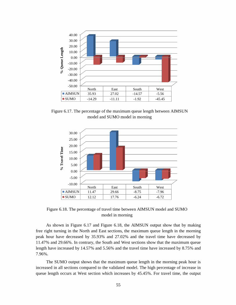
55

Figure 6.17. The percentage of the maximum queue length between AIMSUN model and SUMO model in morning

Figure 6.18. The percentage of travel time between AIMSUN model and SUMO model in morning

As shown in Figure 6.17 and Figure 6.18, the AIMSUN output show that by making free right turning in the North and East sections, the maximum queue length in the morning peak hour have decreased by 35.93% and 27.02% and the travel time have decreased by 11.47% and 29.66%. In contrary, the South and West sections show that the maximum queue length have increased by 14.57% and 5.56% and the travel time have increased by 8.75% and 7.96%.

The SUMO output shows that the maximum queue length in the morning peak hour is increased in all sections compared to the validated model. The high percentage of increase in queue length occurs at West section which increases by 45.45%. For travel time, the output

-50.00-40.00-30.00-20.00-10.00

0.0010.0020.0030.0040.00

North East South WestAIMSUN 35.93 27.02 -14.57 -5.56SUMO -14.29 -11.11 -1.92 -45.45

% Q

ueue

Len

gth

-10.00

-5.00

0.00

5.00

10.00

15.00

20.00

25.00

30.00

North East South WestAIMSUN 11.47 29.66 -8.75 -7.96SUMO 12.12 17.76 -6.24 -6.72

% T

rave

l Tim

e

56

shows similar result with AIMSUN model. The travel time have decreased by 12.12% and 17.76% in the North and East sections, while in the South and West sections, the result shows the travel time have increased by 6.24% and 6.72%.

The comparison of simulation between AIMSUN model output and SUMO model output in the afternoon peak hour can be seen in the Figure 6.19 and Figure 6.20.

Figure 6.19. The percentage of the maximum queue length between AIMSUN model and SUMO model in afternoon

Figure 6.20. The percentage of travel time between AIMSUN model and SUMO model in afternoon

As shown in Figure 6.19 and Figure 6.10, the AIMSUN and SUMO models show that the maximum queue length and the travel time in afternoon peak hour is decreased in almost all sections compared to the validated model. In contrary, the SUMO output shows the queue length have increased of 2.26% in the West section.

-5.00

0.00

5.00

10.00

15.00

20.00

25.00

30.00

35.00

North East South WestAIMSUN 32.02 26.88 9.91 2.15SUMO 2.08 16.67 6.67 -2.26

% Q

ueue

Len

gth

0.00

5.00

10.00

15.00

20.00

25.00

30.00

35.00

40.00

North East South WestAIMSUN 36.09 18.84 5.45 5.95SUMO 15.50 11.98 1.63 1.66

% T

rave

l Tim

e

57

Based on the results above, it can be concluded that the AIMSUN output have no significance differences compared to the SUMO output, although the value of percentages are not similar.

59

VII. CONCLUSION

In this research, AIMSUN modelling of the Idrottsparken roundabout was carried out in order to visualise and evaluate the operating conditions of the roundabout. For this purpose, traffic survey on all four approaches of the roundabout was carried out to collect data on traffic count (with due consideration to vehicle type and turning movement). The road network including geometric configuration was reproduced in the software and the time dependent traffic demand was incorporated into the system in terms of O-D matrices. The simulation model was checked for errors, followed by calibration of parameters and validation the model.

The main goal of this project is to reduce congestion in Idrottsparken roundabout in the morning and the afternoon peak hour due to the most congested traffic. The reduction of congestion is indicated by the reduction of queue length and travel time. This project proposes three alternative scenarios for improving the traffic performance. The first scenario is adding one free right turns in North and East section. In the morning peak hour, although this scenario is able to reduce the queue length and the travel time in North and East sections, this scenario has not been able to reduce the queue length and the travel time in the South and West sections. In the afternoon peak hour, this scenario is able to improve the performance of the roundabout by decreasing the queue length and the travel time in all sections. The second scenario is adding one free right turns in East and South section. In the morning peak hour, this scenario is only able to reduce the queue length and the travel time in East and South sections but this scenario has not been able to reduce the queue length and the travel time in North and West section. Similar with the first scenario, in the afternoon peak hour this scenario is able to improve the performance of the roundabout by decreasing the queue length and the travel time in all sections. The third scenario is adding one lane on Idrottsparken roundabout. This scenario is not able to improve the performance of the roundabout. The best alternative scenario recommended in this project is scenario 1 because compared with scenario 2 this alternative is more significant in reducing the queue length and travel time in almost all sections which is 3 of 4 sections. All of scenarios have disadvantages in the high cost of investment.

The comparison between AIMSUN and SUMO for the same scenario shows that the results have no significance differences. In morning peak hour, AIMSUN output shows the reduction for the queue length and travel time occur in North and East sections compared to the validated model. In contrary, the maximum queue length and travel time are increased in South and West sections. In SUMO model, the maximum queue length in the morning peak hour is increased in all sections compared to the validated model. For travel time, the output shows similar result with AIMSUN model. In afternoon peak hour, the AIMSUN and SUMO models show that the maximum queue length and the travel time are decreased in almost all sections compared to the validated model. In contrary, the SUMO output shows the queue length have increased in the West section. As generally, AIMSUN result gives more significant decrease compared to SUMO model. It can be occurred due to in modelling of

60

roundabouts and complex intersection, AIMSUN result provide high level precision compared to SUMO.

This research is conducted in limited time, limited human resources and also focused on the roundabout at Idrottsparken without considering the minor junctions and side frictions along the street, so the proposed scenarios are also limited. In the next research, a broader scope area could be applied so other alternatives such as using signalized at Idrottsparken roundabout can be taken into consideration.

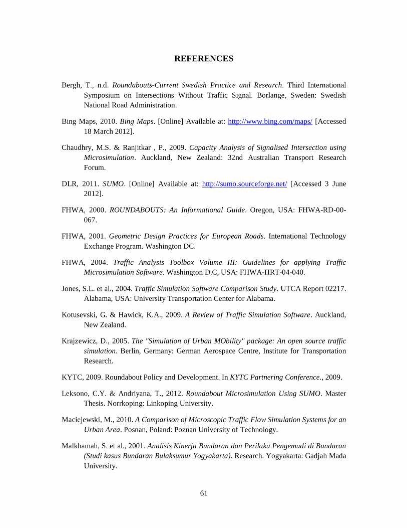
61

REFERENCES

Bergh, T., n.d. Roundabouts-Current Swedish Practice and Research. Third International Symposium on Intersections Without Traffic Signal. Borlange, Sweden: Swedish National Road Administration.

Bing Maps, 2010. Bing Maps. [Online] Available at: http://www.bing.com/maps/ [Accessed 18 March 2012].

Chaudhry, M.S. & Ranjitkar , P., 2009. Capacity Analysis of Signalised Intersection using Microsimulation. Auckland, New Zealand: 32nd Australian Transport Research Forum.

DLR, 2011. SUMO. [Online] Available at: http://sumo.sourceforge.net/ [Accessed 3 June 2012].

FHWA, 2000. ROUNDABOUTS: An Informational Guide. Oregon, USA: FHWA-RD-00-067.

FHWA, 2001. Geometric Design Practices for European Roads. International Technology Exchange Program. Washington DC.

FHWA, 2004. Traffic Analysis Toolbox Volume III: Guidelines for applying Traffic Microsimulation Software. Washington D.C, USA: FHWA-HRT-04-040.

Jones, S.L. et al., 2004. Traffic Simulation Software Comparison Study. UTCA Report 02217. Alabama, USA: University Transportation Center for Alabama.

Kotusevski, G. & Hawick, K.A., 2009. A Review of Traffic Simulation Software. Auckland, New Zealand.

Krajzewicz, D., 2005. The "Simulation of Urban MObility" package: An open source traffic simulation. Berlin, Germany: German Aerospace Centre, Institute for Transportation Research.

KYTC, 2009. Roundabout Policy and Development. In KYTC Partnering Conference., 2009.

Leksono, C.Y. & Andriyana, T., 2012. Roundabout Microsimulation Using SUMO. Master Thesis. Norrkoping: Linkoping University.

Maciejewski, M., 2010. A Comparison of Microscopic Traffic Flow Simulation Systems for an Urban Area. Posnan, Poland: Poznan University of Technology.

Malkhamah, S. et al., 2001. Analisis Kinerja Bundaran dan Perilaku Pengemudi di Bundaran (Studi kasus Bundaran Bulaksumur Yogyakarta). Research. Yogyakarta: Gadjah Mada University.

62

Manstetten, D., Krautter, W. & Schwab, T., 1997. Traffic Simulation Supporting Urban Control System Development. Proceedings of the 4th World conference on ITS, Berlin. Brussel, Belgium.

Mosslemi, M., 2008. Using Metering Signals at Roundabouts with Unbalanced Flow Patterns to Improve the Traffic Condition. Norrkoping, Sweden: Linkoping University.

Nurpandi, I., 2012. Evaluation of Roundabout Using Aimsun Simulation (Case Study Tugu Roundabout In Cianjur, West Java). Master Thesis. Yogyakarta: Gadjah Mada University.

Panwai, S. & Dia, H., 2005. Comparative Evaluation of Microscopic Car-Following Behavior. Queensland, Australia: IEEE Transactions on Intelligent Transportation Systems, Vol. 6, No. 3 The University of Queensland.

TSS, 2010. Microsimulator and Mesosimulator Aimsun 6.1 User's Manual. Barcelona: Copyright @ 1997-2010 TSS-Transport Simulation Systems, S.L.

TSS, 2012. AIMSUN. [Online] Available at: http://www.aimsun.com [Accessed 3 June 2012].

Wikipedia, 2012. Root Mean Square Deviation. [Online] Available at: http://en.wikipedia.org/wiki/Root-mean-square_deviation [Accessed 22 June 2012].

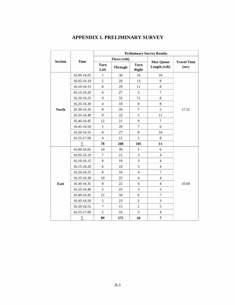
A-1

APPENDIX 1. PRELIMINARY SURVEY

Section Time

Preliminary Survey Results Flows (veh)

Max Queue Length (veh)

Travel Time (sec) Turn

Left Through Turn Right

North

16.00-16.05 1 30 16 10

17.51

16.05-16.10 5 20 13 9 16.10-16.15 8 29 11 8 16.15-16.20 6 27 5 7 16.20-16.25 9 32 11 8 16.25-16.30 4 18 8 8 16.30-16.35 8 26 7 2 16.35-16.40 8 22 5 11 16.40-16.45 12 21 9 7 16.45-16.50 5 20 7 6 16.50-16.55 8 27 8 10 16.55-17.00 4 15 5 8

∑ 78 288 105 11

East

16.00-16.05 10 39 5 6

10.60

16.05-16.10 7 21 3 4 16.10-16.15 9 19 3 4 16.15-16.20 6 18 3 4 16.20-16.25 8 18 4 7 16.25-16.30 10 25 4 4 16.30-16.35 8 22 6 4 16.35-16.40 5 25 3 5 16.40-16.45 12 34 6 7 16.45-16.50 5 23 2 3 16.50-16.55 7 15 2 5 16.55-17.00 2 16 3 4

∑ 89 275 44 7

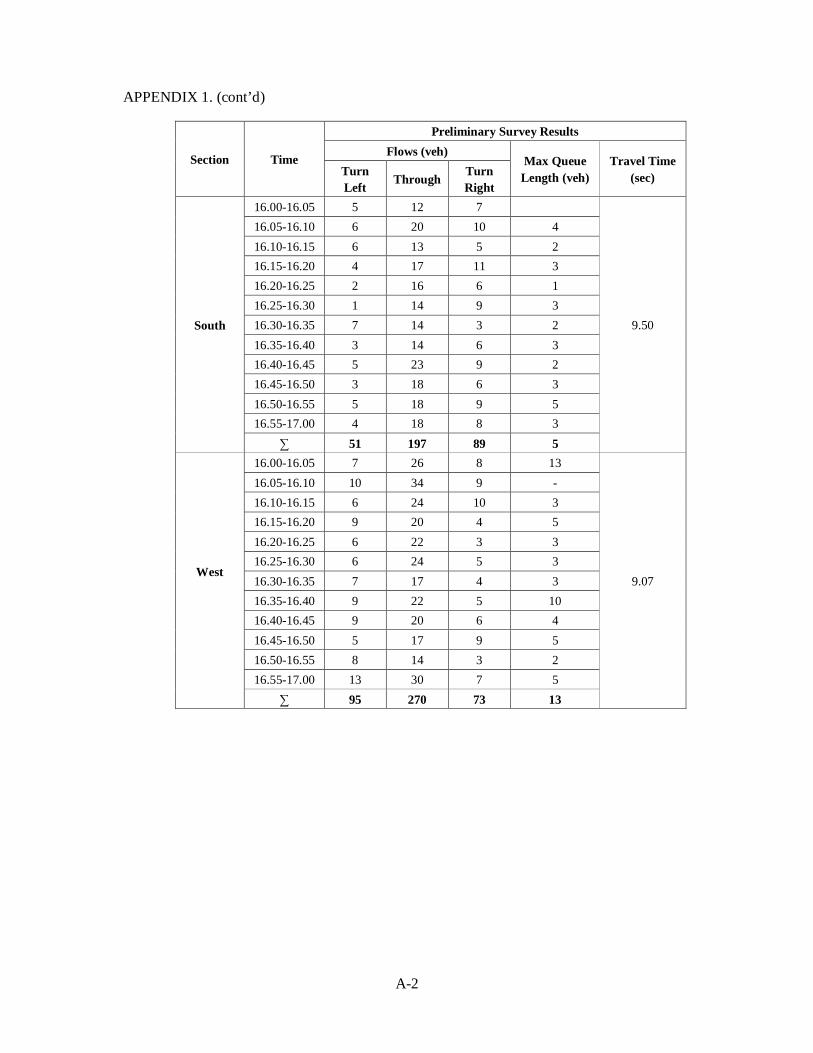
A-2

APPENDIX 1. (cont’d)

Section Time

Preliminary Survey Results Flows (veh)

Max Queue Length (veh)

Travel Time (sec) Turn

Left Through Turn Right

South

16.00-16.05 5 12 7

9.50

16.05-16.10 6 20 10 4 16.10-16.15 6 13 5 2 16.15-16.20 4 17 11 3 16.20-16.25 2 16 6 1 16.25-16.30 1 14 9 3 16.30-16.35 7 14 3 2 16.35-16.40 3 14 6 3 16.40-16.45 5 23 9 2 16.45-16.50 3 18 6 3 16.50-16.55 5 18 9 5 16.55-17.00 4 18 8 3

∑ 51 197 89 5

West

16.00-16.05 7 26 8 13

9.07

16.05-16.10 10 34 9 - 16.10-16.15 6 24 10 3 16.15-16.20 9 20 4 5 16.20-16.25 6 22 3 3 16.25-16.30 6 24 5 3 16.30-16.35 7 17 4 3 16.35-16.40 9 22 5 10 16.40-16.45 9 20 6 4 16.45-16.50 5 17 9 5 16.50-16.55 8 14 3 2 16.55-17.00 13 30 7 5

∑ 95 270 73 13

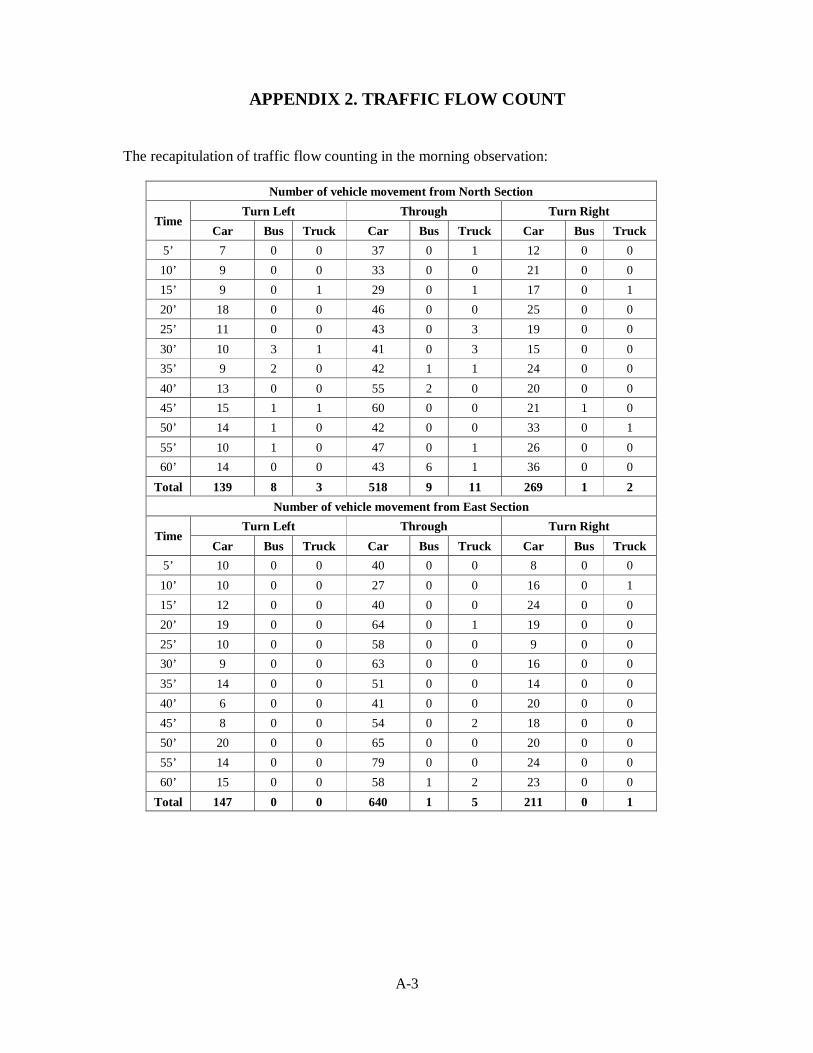
A-3

APPENDIX 2. TRAFFIC FLOW COUNT

The recapitulation of traffic flow counting in the morning observation:

Number of vehicle movement from North Section

Time Turn Left Through Turn Right

Car Bus Truck Car Bus Truck Car Bus Truck 5’ 7 0 0 37 0 1 12 0 0 10’ 9 0 0 33 0 0 21 0 0 15’ 9 0 1 29 0 1 17 0 1 20’ 18 0 0 46 0 0 25 0 0 25’ 11 0 0 43 0 3 19 0 0 30’ 10 3 1 41 0 3 15 0 0 35’ 9 2 0 42 1 1 24 0 0 40’ 13 0 0 55 2 0 20 0 0 45’ 15 1 1 60 0 0 21 1 0 50’ 14 1 0 42 0 0 33 0 1 55’ 10 1 0 47 0 1 26 0 0 60’ 14 0 0 43 6 1 36 0 0

Total 139 8 3 518 9 11 269 1 2 Number of vehicle movement from East Section



Total 147 0 0 640 1 5 211 0 1

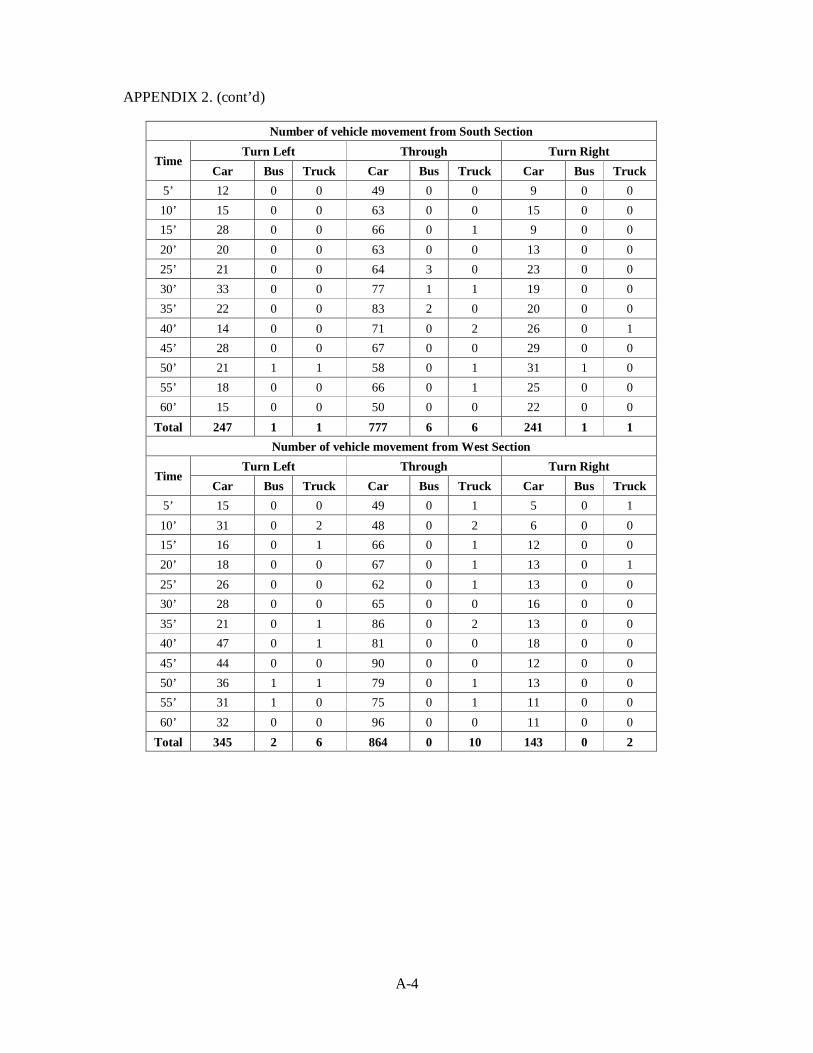
A-4


Number of vehicle movement from South Section



Total 247 1 1 777 6 6 241 1 1 Number of vehicle movement from West Section



Total 345 2 6 864 0 10 143 0 2

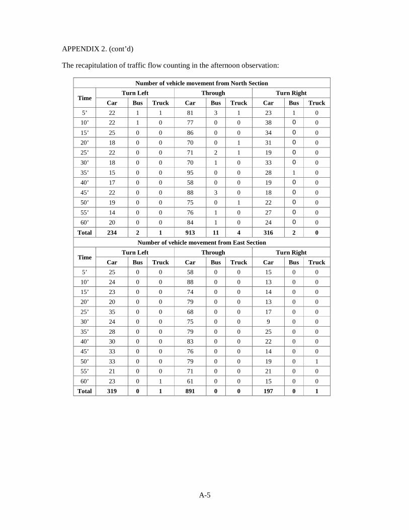
A-5


The recapitulation of traffic flow counting in the afternoon observation:

Number of vehicle movement from North Section


Car Bus Truck Car Bus Truck Car Bus Truck 5’ 22 1 1 81 3 1 23 1 0 10’ 22 1 0 77 0 0 38 0 0 15’ 25 0 0 86 0 0 34 0 0 20’ 18 0 0 70 0 1 31 0 0 25’ 22 0 0 71 2 1 19 0 0

30’ 18 0 0 70 1 0 33 0 0

35’ 15 0 0 95 0 0 28 1 0 40’ 17 0 0 58 0 0 19 0 0

45’ 22 0 0 88 3 0 18 0 0 50’ 19 0 0 75 0 1 22 0 0

55’ 14 0 0 76 1 0 27 0 0 60’ 20 0 0 84 1 0 24 0 0

Total 234 2 1 913 11 4 316 2 0 Number of vehicle movement from East Section



Total 319 0 1 891 0 0 197 0 1

A-6


Number of vehicle movement from South Section



Total 232 0 0 580 8 1 261 0 0 Number of vehicle movement from West Section



Total 272 0 0 914 2 2 278 0 1

A-7

APPENDIX 3. MEAN OF MAXIMUM QUEUE LENGTH

Time

Mean of Maximum Queue Length (veh)

Morning Afternoon

North East South West North East South West

1' - 5' 0.667 2.667 3.000 1.667 5.000 3.000 4.500 4.000

6' - 10' 1.333 2.000 5.000 3.000 6.500 5.000 2.500 2.500

11' - 15' 2.667 4.000 4.667 2.333 4.500 3.000 3.000 3.000

16' - 20' 1.333 3.667 5.000 3.000 7.500 4.000 4.000 6.500

21' - 25' 4.333 5.333 4.000 2.667 8.000 5.500 6.500 4.500

26' - 30' 3.000 6.667 6.000 2.333 6.000 6.500 8.500 2.500

31' - 35' 5.667 6.000 11.667 4.333 5.000 7.000 5.000 3.000

36' - 40' 4.667 7.000 11.000 3.333 4.000 6.500 3.500 2.000

41' - 45' 3.333 8.333 10.000 3.333 8.000 8.000 3.500 3.000

46' - 50' 2.667 7.667 10.000 3.000 4.500 5.000 4.500 5.000

51' - 55' 4.000 8.667 7.000 2.667 7.000 3.500 6.000 1.000

56' - 60' 3.667 5.667 5.000 3.333 1.500 6.000 6.000 2.000

Average 3.111 5.639 6.861 2.917 5.625 5.250 4.792 3.250

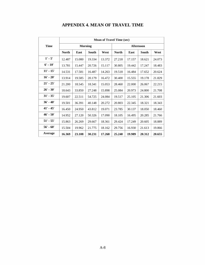
A-8

APPENDIX 4. MEAN OF TRAVEL TIME

Time

Mean of Travel Time (sec)

Morning Afternoon

North East South West North East South West

1' - 5' 12.487 15.080 19.334 13.372 27.218 17.157 18.621 24.073

6' - 10' 13.781 15.447 20.726 15.117 30.805 19.442 17.247 18.483

11' - 15' 14.531 17.581 16.487 14.263 19.518 16.484 17.652 20.624

16' - 20' 13.914 19.585 20.179 16.472 30.400 15.555 19.178 21.829

21' - 25' 21.200 18.545 18.341 15.053 28.460 22.000 26.067 22.215

26' - 30' 18.643 33.850 27.248 15.898 25.084 20.973 24.800 21.708

31' - 35' 19.607 22.511 54.725 24.084 19.517 25.105 21.306 21.603

36' - 40' 19.501 36.391 40.148 20.272 20.803 22.345 18.321 18.343

41' - 45' 16.450 24.950 43.812 19.071 23.785 30.137 18.050 18.460

46' - 50' 14.952 27.120 50.326 17.090 18.105 16.495 20.285 21.766

51' - 55' 15.863 26.269 29.667 18.361 29.424 17.249 20.605 18.889

56' - 60' 15.504 19.962 21.775 18.162 29.756 16.930 21.613 19.866

Average 16.369 23.108 30.231 17.268 25.240 19.989 20.312 20.655

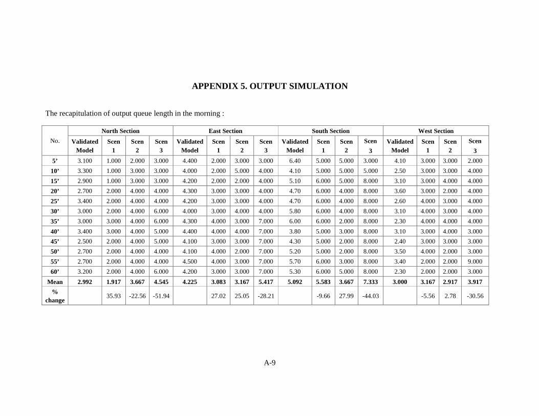
A-9

APPENDIX 5. OUTPUT SIMULATION

The recapitulation of output queue length in the morning :

No. North Section East Section South Section West Section

Validated Model

Scen 1

Scen 2

Scen 3

Validated Model

Scen 1

Scen 2

Scen 3

Validated Model

Scen 1

Scen 2

Scen 3

Validated Model

Scen 1

Scen 2

Scen 3

5’ 3.100 1.000 2.000 3.000 4.400 2.000 3.000 3.000 6.40 5.000 5.000 3.000 4.10 3.000 3.000 2.000 10’ 3.300 1.000 3.000 3.000 4.000 2.000 5.000 4.000 4.10 5.000 5.000 5.000 2.50 3.000 3.000 4.000 15’ 2.900 1.000 3.000 3.000 4.200 2.000 2.000 4.000 5.10 6.000 5.000 8.000 3.10 3.000 4.000 4.000 20’ 2.700 2.000 4.000 4.000 4.300 3.000 3.000 4.000 4.70 6.000 4.000 8.000 3.60 3.000 2.000 4.000 25’ 3.400 2.000 4.000 4.000 4.200 3.000 3.000 4.000 4.70 6.000 4.000 8.000 2.60 4.000 3.000 4.000 30’ 3.000 2.000 4.000 6.000 4.000 3.000 4.000 4.000 5.80 6.000 4.000 8.000 3.10 4.000 3.000 4.000 35’ 3.000 3.000 4.000 6.000 4.300 4.000 3.000 7.000 6.00 6.000 2.000 8.000 2.30 4.000 4.000 4.000 40’ 3.400 3.000 4.000 5.000 4.400 4.000 4.000 7.000 3.80 5.000 3.000 8.000 3.10 3.000 4.000 3.000 45’ 2.500 2.000 4.000 5.000 4.100 3.000 3.000 7.000 4.30 5.000 2.000 8.000 2.40 3.000 3.000 3.000 50’ 2.700 2.000 4.000 4.000 4.100 4.000 2.000 7.000 5.20 5.000 2.000 8.000 3.50 4.000 2.000 3.000 55’ 2.700 2.000 4.000 4.000 4.500 4.000 3.000 7.000 5.70 6.000 3.000 8.000 3.40 2.000 2.000 9.000 60’ 3.200 2.000 4.000 6.000 4.200 3.000 3.000 7.000 5.30 6.000 5.000 8.000 2.30 2.000 2.000 3.000

Mean 2.992 1.917 3.667 4.545 4.225 3.083 3.167 5.417 5.092 5.583 3.667 7.333 3.000 3.167 2.917 3.917 %

change 35.93 -22.56 -51.94 27.02 25.05 -28.21 -9.66 27.99 -44.03 -5.56 2.78 -30.56

A-10


The recapitulation of output queue length in the afternoon :

No. North Section East Section South Section West Section

Validated Model

Scen 1

Scen 2

Scen 3

Validated Model

Scen 1

Scen 2

Scen 3

Validated Model

Scen 1

Scen 2

Scen 3

Validated Model

Scen 1

Scen 2

Scen 3

5’ 5.100 2.000 4.000 7.000 3.300 2.000 3.000 3.000 4.40 3.000 2.000 2.000 5.30 4.000 5.000 3.000 10’ 3.800 2.000 4.000 8.000 5.400 4.000 3.000 3.000 5.30 4.000 2.000 4.000 5.30 4.000 5.000 3.000 15’ 4.000 4.000 4.000 8.000 4.600 2.000 3.000 3.000 1.80 3.000 2.000 4.000 3.80 5.000 5.000 4.000 20’ 4.400 4.000 4.000 8.000 3.100 4.000 3.000 5.000 3.30 3.000 4.000 8.000 4.60 4.000 4.000 4.000 25’ 5.000 2.000 5.000 8.000 4.300 2.000 3.000 5.000 2.40 4.000 4.000 8.000 5.00 4.000 4.000 4.000 30’ 5.000 3.000 4.000 8.000 4.100 3.000 3.000 5.000 4.20 4.000 4.000 8.000 3.00 4.000 5.000 4.000 35’ 6.200 3.000 5.000 8.000 5.300 3.000 3.000 5.000 4.10 3.000 2.000 8.000 5.10 4.000 3.000 5.000 40’ 3.700 4.000 5.000 7.000 4.000 3.000 5.000 7.000 2.70 3.000 2.000 8.000 3.80 3.000 3.000 5.000 45’ 3.800 4.000 5.000 7.000 3.700 4.000 5.000 7.000 3.20 3.000 3.000 8.000 4.50 3.000 3.000 5.000 50’ 3.900 3.000 5.000 7.000 4.200 4.000 5.000 7.000 5.70 4.000 3.000 8.000 3.00 5.000 3.000 7.000 55’ 5.800 4.000 4.000 7.000 4.100 3.000 5.000 7.000 3.60 3.000 3.000 8.000 4.50 5.000 3.000 7.000 60’ 5.200 3.000 4.000 7.000 4.500 3.000 5.000 7.000 3.70 3.000 3.000 8.000 3.20 5.000 5.000 11.000

Mean 4.658 3.167 4.417 7.500 4.217 3.083 3.833 5.333 3.700 3.333 2.833 6.833 4.258 4.167 4.000 5.167 %

change 32.02 5.19 -61.00 26.88 9.09 -24.68 9.91 23.42 -84.68 2.15 6.07 -21.33

A-11


The recapitulation of output travel time in the morning :

No North Section East Section South Section West Section

Validated Model

Scen 1

Scen 2

Scen 3

Validated Model

Scen 1

Scen 2

Scen 3

Validated Model

Scen 1

Scen 2

Scen 3

Validated Model

Scen 1

Scen 2

Scen 3

5’ 15.520 13.110 15.920 18.590 28.480 18.580 16.920 28.500 28.790 29.020 18.250 30.330 20.700 20.760 21.390 29.160 10’ 16.700 13.210 17.670 17.780 25.780 18.490 17.160 27.570 21.740 35.460 19.390 29.340 18.460 24.050 20.440 30.180 15’ 15.910 13.130 18.970 23.020 26.150 19.980 18.040 28.510 24.570 32.010 18.740 39.110 20.590 20.400 20.730 28.530 20’ 16.040 17.590 19.880 24.560 26.270 20.310 17.810 30.080 23.530 26.050 17.330 29.750 14.340 24.550 20.830 27.070 25’ 15.990 12.960 18.630 18.010 26.490 18.950 17.020 27.420 22.230 27.890 17.090 31.000 20.830 22.330 19.980 15.640 30’ 15.690 12.660 16.270 14.980 27.500 16.960 14.930 27.160 27.700 23.460 18.520 28.290 21.980 21.150 21.290 20.910 35’ 15.500 12.010 17.570 19.980 25.990 19.700 17.710 30.970 26.600 24.010 17.650 29.010 15.940 21.490 22.340 15.620 40’ 15.350 14.170 18.280 25.990 27.060 19.500 19.650 30.450 20.460 22.260 17.570 30.950 25.340 22.120 20.540 24.570 45’ 15.230 16.310 18.200 17.720 26.360 18.390 18.620 31.220 22.150 22.560 16.960 30.670 16.230 19.520 19.320 19.160 50’ 14.820 16.340 16.230 21.130 26.890 18.740 16.850 30.370 24.000 26.510 17.390 33.100 20.820 19.440 20.540 16.120 55’ 15.490 13.310 16.060 18.580 28.960 19.620 18.540 28.640 25.090 25.800 19.440 36.710 22.700 19.850 18.790 17.320 60’ 17.340 13.040 16.260 18.360 27.570 18.330 15.910 27.100 22.800 19.970 18.510 33.690 18.530 19.620 20.450 19.320

Mean 15.798 13.987 17.495 19.892 26.958 18.963 17.430 28.999 24.138 26.250 18.070 31.829 19.705 21.273 20.553 21.967 %

change 11.47 -10.74 -25.91 29.66 35.34 -7.57 -8.75 25.14 -31.86 -7.96 -4.31 -11.48

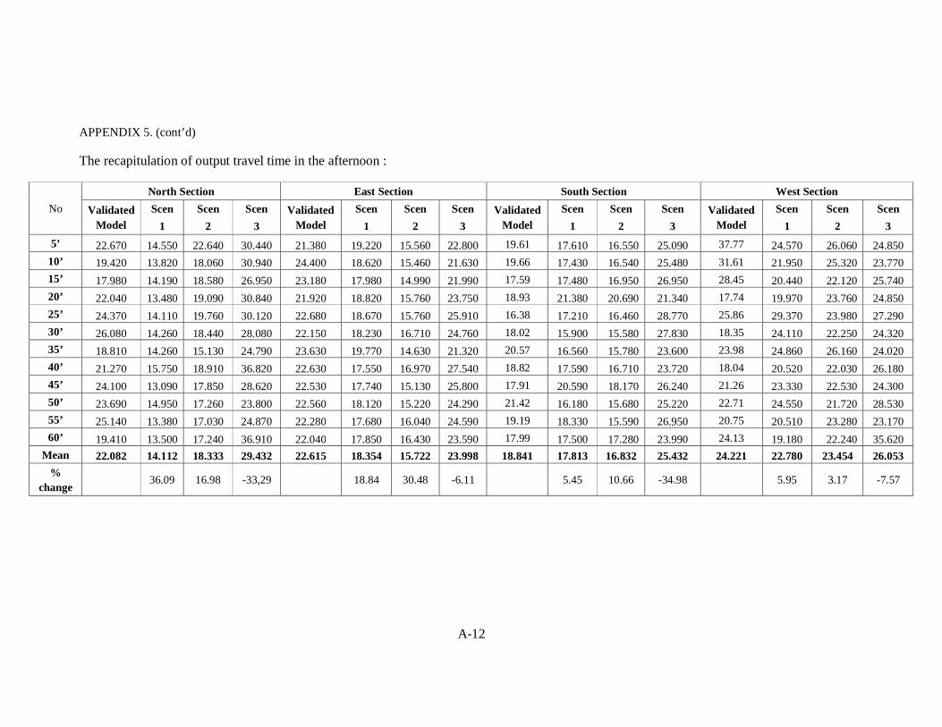
A-12


The recapitulation of output travel time in the afternoon :

No North Section East Section South Section West Section

Validated Model

Scen 1

Scen 2

Scen 3

Validated Model

Scen 1

Scen 2

Scen 3

Validated Model

Scen 1

Scen 2

Scen 3

Validated Model

Scen 1

Scen 2

Scen 3

5’ 22.670 14.550 22.640 30.440 21.380 19.220 15.560 22.800 19.61 17.610 16.550 25.090 37.77 24.570 26.060 24.850 10’ 19.420 13.820 18.060 30.940 24.400 18.620 15.460 21.630 19.66 17.430 16.540 25.480 31.61 21.950 25.320 23.770 15’ 17.980 14.190 18.580 26.950 23.180 17.980 14.990 21.990 17.59 17.480 16.950 26.950 28.45 20.440 22.120 25.740 20’ 22.040 13.480 19.090 30.840 21.920 18.820 15.760 23.750 18.93 21.380 20.690 21.340 17.74 19.970 23.760 24.850 25’ 24.370 14.110 19.760 30.120 22.680 18.670 15.760 25.910 16.38 17.210 16.460 28.770 25.86 29.370 23.980 27.290 30’ 26.080 14.260 18.440 28.080 22.150 18.230 16.710 24.760 18.02 15.900 15.580 27.830 18.35 24.110 22.250 24.320 35’ 18.810 14.260 15.130 24.790 23.630 19.770 14.630 21.320 20.57 16.560 15.780 23.600 23.98 24.860 26.160 24.020 40’ 21.270 15.750 18.910 36.820 22.630 17.550 16.970 27.540 18.82 17.590 16.710 23.720 18.04 20.520 22.030 26.180 45’ 24.100 13.090 17.850 28.620 22.530 17.740 15.130 25.800 17.91 20.590 18.170 26.240 21.26 23.330 22.530 24.300 50’ 23.690 14.950 17.260 23.800 22.560 18.120 15.220 24.290 21.42 16.180 15.680 25.220 22.71 24.550 21.720 28.530 55’ 25.140 13.380 17.030 24.870 22.280 17.680 16.040 24.590 19.19 18.330 15.590 26.950 20.75 20.510 23.280 23.170 60’ 19.410 13.500 17.240 36.910 22.040 17.850 16.430 23.590 17.99 17.500 17.280 23.990 24.13 19.180 22.240 35.620

Mean 22.082 14.112 18.333 29.432 22.615 18.354 15.722 23.998 18.841 17.813 16.832 25.432 24.221 22.780 23.454 26.053 %

change 36.09 16.98 -33,29 18.84 30.48 -6.11 5.45 10.66 -34.98 5.95 3.17 -7.57

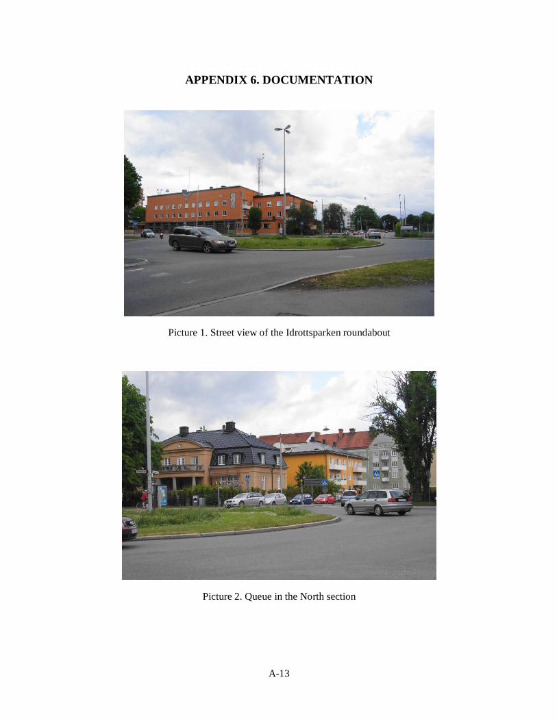
A-13

APPENDIX 6. DOCUMENTATION

Picture 1. Street view of the Idrottsparken roundabout

Picture 2. Queue in the North section

A-14


Picture 3. Queue in the East section

Picture 4. Queue in the South section

A-15


Picture 5. Queue in the West section

MICRO-SIMULATION OF THE ROUNDABOUT AT IDROTTSPARKEN USING AIMSUN551346/FULLTEXT03.pdf ·...

Documents

Transcript of MICRO-SIMULATION OF THE ROUNDABOUT AT IDROTTSPARKEN USING AIMSUN551346/FULLTEXT03.pdf ·...