Micro Grid

IEEE JOURNAL OF EMERGING AND SELECTED TOPICS IN POWER ELECTRONICS, VOL. 2, NO. 1, MARCH 2014 115

DC Microgrid for Wind and Solar Power IntegrationKai Strunz, Ehsan Abbasi, and Duc Nguyen Huu

Abstract— Operational controls are designed to support theintegration of wind and solar power within microgrids. Anaggregated model of renewable wind and solar power generationforecast is proposed to support the quantification of the opera-tional reserve for day-ahead and real-time scheduling. Then, adroop control for power electronic converters connected to bat-tery storage is developed and tested. Compared with the existingdroop controls, it is distinguished in that the droop curves are setas a function of the storage state-of-charge (SOC) and can becomeasymmetric. The adaptation of the slopes ensures that the poweroutput supports the terminal voltage while at the same keepingthe SOC within a target range of desired operational reserve.This is shown to maintain the equilibrium of the microgrid’sreal-time supply and demand. The controls are implemented forthe special case of a dc microgrid that is vertically integratedwithin a high-rise host building of an urban area. Previouslyuntapped wind and solar power are harvested on the roof andsides of a tower, thereby supporting delivery to electric vehicleson the ground. The microgrid vertically integrates with the hostbuilding without creating a large footprint.

Index Terms— Distributed energy resources, droop control,electric vehicle (EV), emission constraint, fast charging,microgrid, multilevel energy storage, optimal scheduling, powerelectronic conversion, solar power, wind power.

NOMENCLATURE

AcronymsBESS Battery energy storage system.dc Direct current.EV Electric vehicle.MES Multilevel energy storage.NR Negative energy reserve of BESS.PR Positive energy reserve of BESS.PV Photovoltaics.RES Renewable energy sources.SOC State of charge.UPS Uninterruptible power supply.WECS Wind energy conversion system.

Variables and OperatorsC Cost of energy.DOD Depth of discharge.EBESS State of charge of BESS.EBESS-0 Initial state of charge of BESS.

Manuscript received August 15, 2013; accepted September 16, 2013. Dateof publication December 11, 2013; date of current version January 29, 2014.Recommended for publication by Associate Editor Wenzhong Gao.

The authors are with the Department of Electrical Engineering, TechnicalUniversity of Berlin, Berlin 10587, Germany (e-mail: [email protected];[email protected]; [email protected]).

Color versions of one or more of the figures in this paper are availableonline at http://ieeexplore.ieee.org.

Digital Object Identifier 10.1109/JESTPE.2013.2294738

ECBESS Energy capacity of BESS.ECNR-3h Energy capacity allocated for negative reserve in

3-h window.ECPR-3h Energy capacity allocated for positive reserve in

3-h window.ECUPS Energy capacity reserved for UPS service.ECEVF Energy capacity for fast charging demand.EMS Emission in system for 1 kWh power generation.EPBF Emission penalty–bonus factor.F Objective function of microgrid optimized

scheduling.i, j Counters for hour and minute.K Number of individual states.L Number of combined states giving an aggregated

state.l, m, n Counters for states.M Number of aggregated states.N Number of combined states.P Power.T Scheduling horizon of optimization.TEVS Scheduling horizon of EV smart charging.t Time.V Voltage.� Difference operator.γ Droop power multiplier for asymmetric droop.ηch, ηdis Charging and discharging efficiency of BESS.τh Time step size equal to 1 h.τmin Time step size equal to 1 min.

Special Designations

x− Lower boundary of x .x+ Upper boundary of x .x Average of x .x̃ Forecast of x .

Subscripts

A Aggregated model of power forecast.BC, GC Battery and grid critical voltage in droops.Bm1, Gm1 Battery and grid marginal level 1 voltage.Bm2, Gm2 Battery and grid marginal level 2 voltage.ch Charging.D Droop.dis Discharging.EVF Electric vehicle fast charging.EVS Electric vehicle smart charging.G Grid.SCap Supercapacitor.1kWh 1kWh electric energy.3h Three successive hours.

2168-6777 © 2013 IEEE. Translations and content mining are permitted for academic research only. Personal use is also permitted,but republication/redistribution requires IEEE permission. See http://www.ieee.org/publications_standards/publications/rights/index.html for more information.

116 IEEE JOURNAL OF EMERGING AND SELECTED TOPICS IN POWER ELECTRONICS, VOL. 2, NO. 1, MARCH 2014

I. INTRODUCTION

IN THE year 2012, 44.8 GW of new wind energy con-version systems were installed worldwide [1]. The trend

has been toward increasingly larger turbine sizes, culminatingin the installation of off-shore wind parks that are locatedfar from the load centers [2]. This can lead to rather largedistances between generation and load in the electricity sector.The transportation sector reveals an even larger disconnectbetween the locations of fuel production and consumption.The energy system proposed in this paper seeks to addressboth issues related to electricity and transportation sectors.One potential solution is a microgrid that can be verticallyintegrated with a high-rise building as frequently encounteredin urban areas. The harvesting of renewable wind and solarenergy occurs at the top of the building. The rooftop generationconnects to the ground level via a microgrid where electricvehicle (EV) charging stations are supplied, and a batterysupports maintaining the balance of supply and demand. Thepotential value of an urban integration within buildings asconsidered here comes from the usage of rooftop energyresources, the storage of the latter for offering EV fast chargingat the ground level, the contribution to emission-free EVtransportation in urban areas, the co-location and integrationof generation and load in urban areas, and the grid-friendlyintegration of the microgrid with the rest of the power systemmain grid.

The combination of wind and solar energy resources ona rooftop was also investigated in [3]. It was verified thatthe combination of wind and solar energy leads to reducedlocal storage requirements [4]. The combination of diversebut complementary storage technologies in turn can form amultilevel energy storage, where a supercapacitor or flywheelprovides cache control to compensate for fast power fluctua-tions and to smoothen the transients encountered by a batterywith higher energy capacity [5], [6]. Microgrids or hybridenergy systems have been shown to be an effective structurefor local interconnection of distributed renewable generation,loads, and storage [7]–[12].

Recent research has considered the optimization of theoperation on one hand [13]–[15] and the usage of dc to linkthe resources on the other [16]–[18]. The dc link voltage wasshown to be maintained by a droop control that relates thedc link voltage to the power output of controllable resources.In this paper, it is proposed to set the droop as a function ofthe expected state of charge (SOC) of the battery accordingto its operational optimization set point versus the actual real-time SOC. The proposed operational optimization is furtherdistinguished in that it quantifies the uncertainty associatedwith renewable generation forecast, emission constraints, andEV fast charging.

Following this introduction, an outline of the principleof a dc microgrid is given in Section II. In Section III,a method is developed for quantifying the aggregatedwind and solar power forecast uncertainty, the resultingrequired SOC of the battery, and the operational optimiza-tion. The optimization-guided droop control is dealt within Section IV. A case study involving a time series and

Fig. 1. Layout of the dc microgrid.

Fig. 2. Wind and PV-based power generation for the vertically integratedmicrogrid.

simulation over diverse time scales to substantiate the claimsmade is discussed in Section V. Conclusions are drawnin Section VI.

II. OUTLINE OF DC MICROGRID

A schematic of the dc microgrid with the conventionsemployed for power is given in Fig. 1. The dc bus connectswind energy conversion system (WECS), PV panels, multi-level energy storage comprising battery energy storage system(BESS) and supercapacitor, EV smart charging points, EV fastcharging station, and grid interface. The WECS is connectedto the dc bus via an ac–dc converter. PV panels are connectedto the dc bus via a dc–dc converter. The BESS can be realizedthrough flow battery technology connected to the dc bus viaa dc–dc converter. The supercapacitor has much less energycapacity than the BESS. Rather, it is aimed at compensatingfor fast fluctuations of power and so provides cache controlas detailed in [19].

Thanks to the multilevel energy storage, the intermittentand volatile renewable power outputs can be managed, and adeterministic controlled power to the main grid is obtained byoptimization. Providing uninterruptible power supply (UPS)

STRUNZ et al.: DC MICROGRID FOR WIND AND SOLAR POWER INTEGRATION 117

Fig. 3. Overview of optimized scheduling approach.

service to loads when needed is a core duty of the urbanmicrogrid. EV fast charging introduces a stochastic load to themicrogrid. The multilevel energy storage mitigates potentialimpacts on the main grid.

In building integration, a vertical axis wind turbine may beinstalled on the rooftop as shown in Fig. 2. PV panels can beco-located on the rooftop and the facade of the building. Suchor similar configurations benefit from a local availability ofabundant wind and solar energy. The fast charging station isrealized for public access at the ground level. It is connectedclose to the LV–MV transformer to reduce losses and voltagedrop. EVs parked in the building are offered smart chargingwithin user-defined constraints.

III. OPERATIONAL OPTIMIZATION OF MICROGRID

FOR RENEWABLE ENERGY INTEGRATION

The algorithm for optimized scheduling of the microgridis depicted in Fig. 3. In the first stage, wind and solarpower generation are forecast. The uncertainty of the windand solar power is presented by a three-state model. Anexample of such a forecast is shown in Fig. 4. State 1represents a power forecast lower than the average powerforecast. This state is shown by the power forecast of ˜P1 withthe forecast probability of p̃r1 assigned to it. The averagepower forecast and the probability of forecast assigned toit give state 2. State 3 represents a power forecast higherthan the average power forecast. Then, wind and solar powerforecasts are aggregated to produce the total renewable powerforecast model. This aggregation method is formulated inSection III-A. The aggregated power generation data are usedto assign hourly positive and negative energy reserves to theBESS for the microgrid operation. The positive energy reserveof the BESS gives the energy stored that can be readilyinjected into the dc bus on demand. The negative energyreserve gives the part of the BESS to remain uncharged tocapture excess power on demand. Energy reserve assessmentis performed according to the aggregated renewable powergeneration forecast. In order to compensate for the uncertaintyof the forecast, a method is devised to assess positive and neg-ative energy reserves in Section III-B. Finally, the emission-constrained cost optimization is formulated to schedule themicrogrid resources for the day-ahead dispatch. The optimizedscheduling is formulated in Section III-C.

Fig. 4. Wind or solar power forecast uncertainty for 1 h.

TABLE I

EXAMPLE A: WIND AND SOLAR POWER FORECAST DATA

Fig. 5. Aggregation of wind and solar power forecast in microgrid.

A. Aggregated Model of Wind and Solar Power Forecast

Wind and solar power generation forecast uncertainty dataare made available for the urban microgrid. Specifically, asshown in Fig. 4, the output power state and the probabilityassigned to that state are available. In the three-state model,the number of individual states is K = 3. A sample of forecastdata of the wind and solar power generation is provided for1 h, as shown in Table I. For example, at a probability of 50%the wind power will be 50 kW in state 2.

The aggregation of output power states of the wind andsolar power is formed as follows. As the microgrid has twogeneration resources with three individual states, K = 3,the number of combined states is N = K 2, which is equalto nine in this case. The combined states in the forecastuncertainty model of wind and solar power are shown in Fig. 5.In each combined state, the power of those individual statesis summed up, and the probability of a combined state is theproduct of the probabilities in individual states assuming thatthe individual states are not correlated.

For the wind and PV power forecast shown in Table I,nine combined states are defined. Those states are providedin Table II. The combined states, as shown by the examplein Table II, should be reduced to fewer representative states.To aggregate the combined states, M aggregated states aredefined. In this example M = 3. Those states are shown inTable II and denoted by m. The borders between aggregated


TABLE II

EXAMPLE A: COMBINED STATES OF WIND AND SOLAR POWER FORECAST

states are determined based on the borders between individualstates in Table I. The average renewable power of individualstates 1 and 2 is 62.5 kW and gives the border betweenaggregated states 1 and 2. Likewise, the average renewablepower of individual states 2 and 3 gives the border betweenaggregated states 2 and 3.

If an aggregated state m covers a number of combinedstates L, the probability of having one of those aggregatedstates is the sum of the probabilities of those combined states

p̃rA,m =L

∑

l=1

p̃r l,m (1)

where p̃rA,m is the forecast probability of renewable power atthe aggregated state m, and p̃r l,m is the forecast probability ofrenewable power at the combined state l within the aggregatedstate m. The average power of each aggregated state iscalculated by the average weighting of all power outputs inthe aggregated state m

˜PA,m =∑L

l=1 p̃r l,m × ˜Pl,m

p̃rA,m(2)

where ˜PA,m is the power forecast of renewables at the aggre-gated state m, and ˜Pl,m is the power forecast at the combinedstate l within the aggregated state m.

In the example shown in Table II, the combined model isreduced to a three-state wind and solar power forecast model.Employing (1) and (2), the calculation is shown for aggregatedstate 1 in the following:

p̃rA,1 = 0.0625 + 0.1250 = 0.1875

˜PA,1 = 55 × 0.0625 + 60 × 0.1250

0.1875kW

= 58.33 kW.

A summary of the aggregated three-state model for the renew-able power generation is provided in Table III. In this table,the power output at state 2 represents the average renewableenergy source power forecast and is used for optimizedscheduling. This three-state model is chosen as an illustrativeexample because it is the minimum model to represent powergeneration forecast uncertainty. More states may be used ifdeemed appropriate.

The aggregated output power states are employed to calcu-late required hourly positive and negative energy reserves in

TABLE III

EXAMPLE A: SINGLE HOUR OF AGGREGATED THREE-STATE POWER

FORECAST MODEL

TABLE IV

EXAMPLE B: THREE HOURS OF AGGREGATED THREE-STATE POWER

FORECAST MODEL

the BESS for operation of the urban microgrid. An exampleon how to use the aggregated three-state power forecast modelto determine hourly positive and negative energy reserves inthe BESS is provided in the following.

B. Energy Reserve Assessment for Operation of Microgrid

Taking into account the aggregated wind and solar powerforecast model developed above, an illustrative exampleis provided to show how the energy reserve is assessed.In Table IV, an aggregated three-state power forecastmodel for three continuous hours is assumed. The aggre-gated power forecast for hour 1 is taken from the examplesolved in Section III-A. The aggregated power forecast ofhours 2 and 3 is calculated by the same method.

As shown in Table IV, the probability of having real-timepower output at state 1 in three continuous hours is equal tothe product of the probabilities in state 1 for those three hours.This probability is thus equal to 0.18753 = 0.00659. This isalso the same probability for having state 3 in three continuoushours. The probability is very small. Therefore, the BESS hasenough negative energy reserve to cover for uncertainty forthree successive hours if the following condition is met:

ECNR-3h = (81.67 − 70) kWh + (127.33 − 110) kWh

+(40.83 − 35) kWh

= 34.83 kWh.


Fig. 6. Battery storage capacity allocation for optimized scheduling.

Power at aggregated state 3 represents the power forecasthigher than average, state 2. Therefore, the negative reservethat is used to capture excess energy is calculated by sum-mation of the energy pertaining to state 3 minus the energypertaining to state 2 in a 3-h window. This means that themicrogrid has, at the high probability of 1 − 0.18753, the freecapacity in the BESS to capture the excess of renewable energyfor a 3-h window.

Similar to the negative energy reserve assessment, thepositive energy reserve is assessed. In order to calculate thepositive energy reserve for the example shown in Table IV,energy of state 2 is subtracted from energy of state 1 for allthree hours, and the results are summed up. Positive energyreserve is the stored energy in the BESS ready to be injectedinto the dc bus to mitigate less renewable power generationthan expected

ECPR-3h = (70 − 58.33) kWh + (110 − 92.67) kWh

+(35 − 29.17) kWh

= 34.83 kWh.

Similar to the example solved for 1 h in Table III, theaggregated model should be developed for the whole dispatchperiod. For instance, if the scheduling horizon is 24 h, awindow sweeps the horizon in 24/3 blocks. Thus, eight blocksof reserve will be determined.

Both positive and negative energy reserves are considered inthe BESS energy constraint. Based on the operation strategy,BESS storage capacity allocation is shown in Fig. 6. The depthof discharge (DOD), positive energy reserve (PR), operationalarea, and negative energy reserve (NR) are allocated in theBESS. The BESS can only be charged and discharged in theoperation area in normal operation mode, which is scheduledby optimization. The BESS may operate in positive andnegative energy reserve areas in order to compensate theuncertainties of power generation and load demand in real-time operation.

C. Formulation of Optimized Scheduling of Microgrid

The objective of the optimization is to minimize operationcost of the microgrid in interconnected mode and provideUPS service in the autonomous mode. These objectives can beachieved by minimization of the following defined objectivefunction:

F(PG, PEVS) =T

∑

i=1 h

C1kWh(i) × PG(i) × τh

+T

∑

i=1 h

C1kWh(i) × PEVS(i) × τh

+T

∑

i=1 h

EPBF × EMS × PG(i) × τh (3)

where F is the objective function to be minimized, T is thescheduling horizon of the optimization, τh is the optimizationtime step which is 1 h, C1kWh is the energy cost for 1 kWhenergy, PG is the incoming power from the grid, PEVS is thesmart charging power for EVs, EPBF is the emission penalty–bonus factor for CO2, and EMS is the average CO2 emissionof 1 kWh electrical energy in the power system outside themicrogrid. In this objective function, PG and PEVS are to bedetermined by optimization. The first term in the objectivefunction above expresses the energy cost, the second termdefines the cost of EV smart charging, and the third termdescribes the emission cost.

As shown in Fig. 1, for positive values of PG, the microgriddraws power from the main grid, and for negative valuesof PG the microgrid injects power into the main grid. Theemission term penalizes power flow from the main grid tothe microgrid. If the microgrid draws power from the maingrid, the microgrid would contribute to emissions of the powersystem. On the other hand, as the microgrid has no unitthat produces emission, when the microgrid returns powerto the main grid, it contributes to emission reduction. Theoptimization program determines a solution that minimizes theoperation cost of the dc microgrid. Thus, a monetary value isassigned to emission reduction by this approach. This objectivefunction is subject to the constraints as follows.

1) Power limitation of the grid interface introduces aboundary constraint to the optimization

PG− ≤ PG(t) ≤ PG+ ∀t ∈ T (4)

where PG− is the lower boundary of the grid power, andPG+ is the upper boundary of the grid power.

2) The BESS power has to be within the limits

PBESS− ≤ PBESS(t) ≤ PBESS+ ∀t ∈ T (5)

where PBESS− is the lower boundary of the outgoingpower from the BESS to the dc bus, PBESS is the BESSpower to the dc bus, and PBESS+ is the upper boundaryof the BESS power.

3) The availability of EV and charging power limits shouldbe met

0 ≤ PEVS(t) ≤ PEVS+ ∀t ∈ TEVS (6)

where PEVS is the EV charging power, PEVS+ is theupper boundary of the EV charging power, and TEVSgives the hours in which EVs are available for smartcharging.

4) The power balance equation has to be valid at allsimulation time steps

˜PA,2(t) + PBESS(t) + PG(t) − ˜PEVF(t) − PEVS(t) = 0

∀t ∈ T (7)

where ˜PA,2 is the average power forecast of renewableenergy sources wind and solar at aggregated state 2, and˜PEVF is the EV fast charging power forecast.

5) The objective function is also subject to a constraint ofthe SOC of the BESS. In order to include UPS service,the formulation of the optimization is modified. The key


application is supplying loads by the microgrid for adefined time span in the case of a contingency. It isdevised so that the microgrid provides backup power fora commercial load such as a bank branch or an officeduring working hours. According to the system layoutshown in Fig. 1, this constraint can be defined as follows:

EBESS−(t)≤ EBESS-0−t

∑

j=1 min

�EBESS( j) ≤ EBESS+(t)

∀t ∈ T (8)

where EBESS− is the lower boundary of energy capacityof the BESS, EBESS-0 is the SOC of the BESS at thebeginning of the optimization, �EBESS is the dischargedenergy from the BESS to the dc bus at every minute,and EBESS+ is the upper boundary of energy capacityof the BESS. The SOC of the battery at all time stepsshould be in the operation zone of the BESS. Therefore,in this equation, the SOC of the battery is calculated andchecked to be within the upper and lower SOC limits.Quantities EBESS−, EBESS+, and �EBESS are calculatedas follows:

EBESS−(t) = ECBESS × (1 − DOD) + ECPR-3h(t)

+ECUPS(t) + ˜ECEVF(t) ∀t ∈ T (9)

where EBESS− is the lower boundary of BESS SOC,ECBESS is the energy capacity of the BESS, DOD is thedepth of discharge of the BESS, ECPR-3h is the positiveenergy reserve of the BESS to cover power forecastuncertainty, ECUPS is the energy capacity allocated inthe BESS for the UPS service of the loads, and ˜ECEVF isthe energy capacity forecast for fast charging demand.The first term in the equation takes into account thepossible depth of discharge.

The BESS cannot be charged up to the full capacitybecause negative energy reserve is scheduled in theBESS to capture potential excess renewable power ascalculated in Section III-B. This boundary constraint isexpressed by

EBESS+(t) = ECBESS − ECNR-3h(t) ∀t ∈ T (10)

where EBESS+ is the upper boundary of BESS SOC,ECBESS is the energy capacity of the BESS, andECNR-3h is the negative energy reserve of the BESS.

The discharged energy from the BESS to the dc busis calculated by

�EBESS(t)={

PBESS(t)ηdis

× τmin, PBESS ≥ 0PBESS(t) × ηch × τmin, PBESS < 0

(11)

where �EBESS is the discharged energy from the BESSto the dc bus in every minute, ηdis is the dischargingefficiency of the BESS, ηch is the charging efficiency ofthe BESS, and τmin is the time step size equal to 1 min.

6) The total required EV smart charging energy for theday-ahead scheduling is to be met. This is defined by

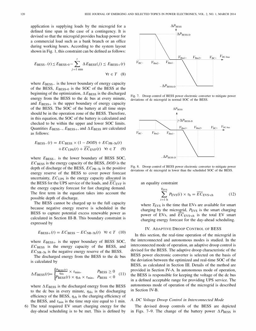
Fig. 7. Droop control of BESS power electronic converter to mitigate powerdeviations of dc microgrid in normal SOC of the BESS.

Fig. 8. Droop control of BESS power electronic converter to mitigate powerdeviations of dc microgrid in lower than the scheduled SOC of the BESS.

an equality constraintTEVS∑

i=1 h

PEVS(i) × τh = ˜ECEVS-ch (12)

where TEVS is the time that EVs are available for smartcharging by the microgrid, PEVS is the smart chargingpower of EVs, and ˜ECEVS-ch is the total EV smartcharging energy forecast for the day-ahead scheduling.

IV. ADAPTIVE DROOP CONTROL OF BESS

In this section, the real-time operation of the microgrid inthe interconnected and autonomous modes is studied. In theinterconnected mode of operation, an adaptive droop control isdevised for the BESS. The adaptive droop characteristic of theBESS power electronic converter is selected on the basis ofthe deviation between the optimized and real-time SOC of theBESS, as calculated in Section III. Details of the method areprovided in Section IV-A. In autonomous mode of operation,the BESS is responsible for keeping the voltage of the dc busin a defined acceptable range for providing UPS service. Theautonomous mode of operation of the microgrid is describedin Section IV-B.

A. DC Voltage Droop Control in Interconnected Mode

The devised droop controls of the BESS are depictedin Figs. 7–9. The change of the battery power �PBESS is


Fig. 9. Droop control of BESS power electronic converter to mitigate powerdeviations of dc microgrid in higher than the scheduled SOC of the BESS.

modified as a function of the dc voltage. It can be noted thattwo of the three devised droop characteristics are asymmetric.The first droop curve, as shown in Fig. 7, is devised fora case where the real-time SOC of the BESS is withinclose range of the optimized SOC of the BESS from thescheduling calculated in Section III-C. The acceptable real-time SOC is determined through definition of upper and lowerboundaries around the optimized SOC. If the real-time SOCis within these boundaries, the droop control of the BESSpower electronic converter is selected as shown in Fig. 7 tosupport the dc voltage. In this case, the upper boundary andthe lower boundary lead to a symmetrical droop response. Inthe voltage range between VBm1− and VBm1+, battery storagedoes not react to the voltage deviations of the dc bus. In thevoltage range from VBm1− to VBm2− and also from VBm1+to VBm2+, the droop control of the BESS reacts. Therefore,�PBESS modifies the power output PBESS to mitigate thevoltage deviation of the dc bus. Finally, in the voltage rangefrom VBm2− to VBC− and also from VBm2+ to VBC+, the droopcurve is in a saturation area, and thus the BESS contributionis at its maximum and constant.

The second droop curve as shown in Fig. 8 is devised for asituation where the real-time SOC of the BESS is lower thanthe optimized and scheduled SOC of the BESS. Therefore, theBESS contributes to stabilizing the dc bus voltage by chargingat the same power as shown in Fig. 7. However, the upperboundary of the BESS droop response is reduced by the factorγ, and it is equal to γ ·�PBESS-D. This way, the SOC can comecloser to the optimized and scheduled SOC.

The third droop curve as shown in Fig. 9 is devised for asituation where the real-time SOC of the BESS is higher thanthe optimized and scheduled SOC of the BESS. Therefore,the BESS contributes to stabilizing the dc bus voltage bydischarging at the same power as shown in Fig. 7. However,the lower boundary of the BESS droop response is modifiedby the factor γ, and it is equal to −γ · �PBESS-D.

The dc–ac converter connected to the main grid is also con-trolled by a droop, as shown in Fig. 10. The droop parametersare adjusted to support the droop control of the storage. Theboundaries must respect the capacity of the converter.

In real-time operation and interconnected mode, the SOCof the BESS is measured and compared against the optimizedSOC of the BESS, and the proper droop will be selected as

Fig. 10. Droop control of the grid power electronic converter in intercon-nected operation mode of dc microgrid.

TABLE V

ADAPTIVE DROOP SELECTION FOR THE BESS

described above. A summary of the droop selection for theBESS in interconnected operation mode is shown in Table V.

B. DC Voltage Droop Control in Autonomous Mode

In the autonomous mode, the main grid is disconnected.Then, the fast charging service has less priority compared withthe supply of other loads. The control of the BESS converteris also defined by the voltage–power droop as discussed. TheBESS so supports the voltage of the dc bus.

V. VERIFICATION BY SIMULATION

The proposed operational method of the urban microgridin day-ahead scheduling and real-time operation is verifiedby simulation. For the day-ahead scheduling, the methodintroduced in this paper is implemented in MATLAB andsimulated for a case study. The real-time operation of the urbanmicrogrid is verified by simulation in PSCAD [20].

A. Simulation of Optimized Scheduling

The optimized scheduling of a vertically integrated urbanmicrogrid with renewable energy harvesting as shown in Fig. 2and EV charging on the ground is verified for the followingassumptions.

1) A vertical axis wind turbine with a generation capacityof 100 kW is installed on the rooftop.

2) Photovoltaic panels with a generation capacity of 50 kWare mounted on the building.

3) A flow battery with the energy capacity of 1000 kWh,power rating of 400 kW, and charging and dischargingefficiencies of 0.95 and 0.90, respectively, is placed inthe basement of the building. The SOC of the BESSat the beginning of the optimization is assumed to


Fig. 11. Case study: Inputs. (a) 1 kWh energy cost profile. (b) Average windand solar power forecast profiles. (c) Fast charging profile of electric vehicles.

be 300 kWh. The DOD of the BESS is 80% of themaximum energy capacity, which gives a minimumpossible discharge to SOC of 200 kWh.

4) A supercapacitor storage with a capacity of 100 kW isinstalled.

5) The BESS and supercapacitor together form a multi-level energy storage, where the supercapacitor providesfast dynamic response under an energy cache controlscheme [19].

6) The dc bus capacitance is distributed among convertersaccording to rating and in sum is 40 mF.

7) A grid interface with the capacity of 300 kW is provided.8) The energy cost diagram for 1 kWh energy is given in

Fig. 11(a).9) The power generation forecast curves of the wind and

PV-based power generation are shown in Fig. 11(b).10) A fast charging station to serve one EV at a time is

provided. The charging power is 100 kW. A uniformdistribution function is employed to simulate the demandof fast charging in each quarter of an hour from 7 AM

to 9 PM. The simulated fast charging profile is providedin Fig. 11(c).

11) The average amount of CO2 emission to generate1 kWh electricity in the power system (EMS) is0.61235 kg/kWh [21]. The emission penalty–bonus

TABLE VI

CASE STUDY: ASSUMED INDIVIDUAL WIND AND SOLAR POWER

FORECAST UNCERTAINTY DATA

Fig. 12. Case study: Three-state aggregated renewable power generationmodel and reserve allocation. (a) Three-state aggregated wind and solar powerforecast profile. (b) Positive and negative energy reserve profiles of BESS.

factor (EPBF) of 3 c$/kg CO2 is chosen for the opti-mization.

12) The UPS service is devised for 50 kW power and 4 hof continuous supply from 8 AM to 4 PM.

13) EVs are available for smart charging from 8 PM to thenext day at 7 AM. The maximum smart charging powerof the aggregated EVs is 20 kW. The daily demand ofEVs is forecasted to be 50 kWh.

Based on the method to aggregate uncertainty of forecastof the renewable resources formulated in Section III-A, thewind and PV power are aggregated. In order to generate theaggregated three-state model for the renewable resources ofthe urban microgrid, forecast uncertainties are assumed asshown in Table VI. In this table, wind and solar power forecasterror data are provided in percentage power deviations fromthe average value in state 2. These data apply to the wind andsolar power profiles as shown in Fig. 11(b).

From the aggregated three-state model shown in Fig. 12(a),based on the method introduced in Section III-A, the 3-h window of positive and negative energy reserves in theBESS is determined as depicted in Fig. 12(b) and explainedin Section III-B. As shown, in each 3-h window starting athour 1, the positive and negative energy reserves are oftenthe same. It can happen that the positive and negative reservesare not equal. This has happened twice for windows coveringhours 7 to 9 and 16 to 18. At hours 9 and 17, wind power as


Fig. 13. Case study: Cost-optimized scheduling of dc microgrid.(a) Optimized scheduling results of the BESS and the grid. BESS and gridpower profiles are in per unit of 500 kW, and BESS energy profile is in perunit of 1000 kWh. (b) Optimized charging profile of EVs.

shown in Fig. 11(b) is at the maximum. Based on the powerrating of the wind turbine, at those hours the output power can-not exceed the nominal value. As a result, the wind power ofstate 2 is equal to the maximum value of power as in state 3.Consequently, less negative reserve is required since the windpower in state 3 is equal to wind power in state 2.

The optimization method is implemented in the MAT-LAB Optimization Toolbox. The active-set algorithm is usedto solve the optimization problem with the linear objec-tive function and the associated constraints. Power limitsof the components are translated into power boundary con-ditions in the implemented optimization code. The powerbalance constraint (7) is implemented as equality constraint.The total required smart EV charging energy (12) is alsoimplemented as an equality constraint. The BESS energyconstraint (8) is implemented by an array of inequalityconstraints.

Simulation results are provided in Fig. 13(a) and (b). Thebattery power delivered to the dc bus of the urban microgrid,SOC of the battery, and power coming from the main gridare given. As shown, the BESS is charged when the energyprice is relatively low. The urban microgrid injects power tothe grid at high energy prices. The urban microgrid is able tosupply all the fast charging demand. From 8 AM to 4 PM, theurban microgrid has adequate SOC to provide 50 kW UPS fora duration of four continuous hours. Thanks to the optimizedoperation strategy, all the objectives of the urban microgridoperation are met.

B. Simulation of Adaptive DC Voltage Droop Control

The layout of the urban microgrid which is implementedin PSCAD [20] is shown in Fig. 1. The power electronic

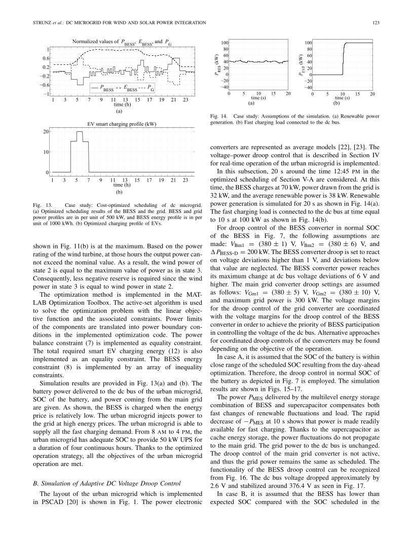
Fig. 14. Case study: Assumptions of the simulation. (a) Renewable powergeneration. (b) Fast charging load connected to the dc bus.

converters are represented as average models [22], [23]. Thevoltage–power droop control that is described in Section IVfor real-time operation of the urban microgrid is implemented.

In this subsection, 20 s around the time 12:45 PM in theoptimized scheduling of Section V-A are considered. At thistime, the BESS charges at 70 kW, power drawn from the grid is32 kW, and the average renewable power is 38 kW. Renewablepower generation is simulated for 20 s as shown in Fig. 14(a).The fast charging load is connected to the dc bus at time equalto 10 s at 100 kW as shown in Fig. 14(b).

For droop control of the BESS converter in normal SOCof the BESS in Fig. 7, the following assumptions aremade: VBm1 = (380 ± 1) V, VBm2 = (380 ± 6) V, and�PBESS-D = 200 kW. The BESS converter droop is set to reacton voltage deviations higher than 1 V, and deviations belowthat value are neglected. The BESS converter power reachesits maximum change at dc bus voltage deviations of 6 V andhigher. The main grid converter droop settings are assumedas follows: VGm1 = (380 ± 5) V, VGm2 = (380 ± 10) V,and maximum grid power is 300 kW. The voltage marginsfor the droop control of the grid converter are coordinatedwith the voltage margins for the droop control of the BESSconverter in order to achieve the priority of BESS participationin controlling the voltage of the dc bus. Alternative approachesfor coordinated droop controls of the converters may be founddepending on the objective of the operation.

In case A, it is assumed that the SOC of the battery is withinclose range of the scheduled SOC resulting from the day-aheadoptimization. Therefore, the droop control in normal SOC ofthe battery as depicted in Fig. 7 is employed. The simulationresults are shown in Figs. 15–17.

The power PMES delivered by the multilevel energy storagecombination of BESS and supercapacitor compensates bothfast changes of renewable fluctuations and load. The rapiddecrease of −PMES at 10 s shows that power is made readilyavailable for fast charging. Thanks to the supercapacitor ascache energy storage, the power fluctuations do not propagateto the main grid. The grid power to the dc bus is unchanged.The droop control of the main grid converter is not active,and thus the grid power remains the same as scheduled. Thefunctionality of the BESS droop control can be recognizedfrom Fig. 16. The dc bus voltage dropped approximately by2.6 V and stabilized around 376.4 V as seen in Fig. 17.

In case B, it is assumed that the BESS has lower thanexpected SOC compared with the SOC scheduled in the


Fig. 15. Case A: Droop-control-based responses to wind fluctuation andfast charging when SOC of battery is as scheduled. (a) Multilevel energystorage system (MES) charging power from the dc bus. (b) Battery chargingpower from the dc bus. (c) Supercapacitor discharging power to the dc bus.(d) Grid power to the dc bus.

Fig. 16. Case A: BESS and grid droop response curves. (a) Droop responsecurve of BESS. (b) Droop response curve of grid.

Fig. 17. Case A: dc bus voltage profile.

optimization. As a result, the BESS droop control as depictedin Fig. 8 is selected. In the new droop control, γ is 0.33. Allother assumptions are the same as in case A where the fastcharging load is connected to the dc bus at time 10 s. Thesimulation results are depicted in Figs. 18–20.

With the asymmetric droop curve of the BESS of Fig. 8,the multilevel energy storage in case B does not provide fullcompensation of renewable fluctuations and the heavy fastcharging EV. So, the droop control of the grid is also activated,and the main grid contributes to the fast charging powerdemand. The BESS power is without fluctuation thanks to the

Fig. 18. Case B: Droop-control-based responses to wind fluctuation and fastcharging when SOC of battery is lower than scheduled. (a) Multilevel energystorage system (MES) charging power from the dc bus. (b) Battery chargingpower from the dc bus. (c) Supercapacitor discharging power to the dc bus.(d) Grid power to the dc bus.

Fig. 19. Case B: BESS and grid droop response curves. (a) Droop responsecurve of BESS. (b) Droop response curve of grid.

Fig. 20. Case B: dc bus voltage profile.

supercapacitor, which absorbs the rapid power fluctuations.The dc bus voltage drops to around 374.4 V as shown inFig. 20. The voltage drop is higher than in case A. This is dueto the wider range of droop control characteristics of the maingrid converter and less contribution of the BESS to voltagecontrol. The functionality of the BESS and grid droop controlcan be recognized from Fig. 19.

The comparison of the results shows the importance of coor-dinating the droop settings with the scheduling in microgridswith wind and solar power. While in Fig. 15 the SOC of thebattery is as desired according to the scheduling, the SOC of


the battery has become lower than expected due to forecastuncertainty in Fig. 18. In the latter case, the asymmetricdroop of Fig. 8 avoids further significant discharging, but hasfull droop contribution on the charging side. On the reduceddischarging side, the droop of the other power electronicconverter connecting to the main grid kicks in to keep upthe dc voltage if necessary. From Fig. 19, it can be seen thatthe droop response of the grid converter becomes active atVDC-bus = 375 V. Above that level, the droop control of theconverter connected to the storage acts on its own. As it doesso at a lower response compared with the case where the SOCis not below the scheduled level, the steady-state ripple ofVDC-bus in the first 10 s is higher in Fig. 20 than it is inFig. 17.

VI. CONCLUSION

A dc microgrid for renewable power integration has beenproposed. The operational optimization and power-electronics-based voltage–power droop control was developed, and thefunctioning was demonstrated through simulation. Interactionwith the main grid was controlled as a result of an opera-tional optimization that seeks to minimize cost and emissions.A method to quantify the uncertainty affiliated with the fore-cast of aggregated wind and PV-based power generation wascreated and used to quantify the energy reserve of the batteryenergy storage system. The battery is parallel-connected witha supercapacitor to form a multilevel energy storage. Thelatter plays a critical role in compensating renewable powerfluctuations and providing the power needed when EVs stop byfor fast charging. In accordance with the microgrid paradigm,operation is also supported in autonomous mode to supportUPS when the connection to the main grid is unavailable.During such periods, fast charging is not supported, as thepriority shifts to supplying critical local loads.

Power electronics is a key enabling technology in con-necting all energy resources to the dc bus. The converterssupport the dc voltage through a droop control scheme. Thecontrol proposed here is adaptive in that the voltage–powerdroop curves are modified depending on the outcome ofthe operational optimization. As a novelty, asymmetric droopcurves were proposed for the converters connected to thestorage so as to also support the objective of bringing theactual battery SOC close to the desired one as scheduled. Thisensures, in particular for the multilevel energy storage, that thecontribution toward dc voltage control does not compromiseits role in providing adequate energy reserve.

For the special case of an urban location, the verticalintegration within a tower building offers renewable wind andsolar power harvesting on the top and energy delivery at thebottom on the ground level, for example for EV charging.The structure contributes to closely co-locating renewablepower generation and delivery to local stationary and mobileEV energy resources.

In sum, this paper contributes to the microgrid paradigmby a novel droop control that takes into account storageSOC when adaptively setting the slopes of the voltage–powerdroop curves; the proposed forecast based on aggregation of

renewable power generation contributes to quantifying energyreserve. In an urban setting, a tower-integrated installationto co-locate harvesting of wind energy and local delivery ofclean energy is an alternative. The optimization for powerexchanges and dc voltage control using adaptive control areperformed through power electronic converters that serve asinterfaces to all resources. The resulting energy system serveslocal stationary and EV-based mobile consumers, and it is agood citizen within the main grid as it reduces emissions bylocal usage of wind and solar energy.

REFERENCES

[1] “Global wind report: Annual market update 2012,” Global Wind EnergyCouncil, Brussels, Belgium, Tech. Rep., 2012.

[2] H. Polinder, J. A. Ferreira, B. B. Jensen, A. B. Abrahamsen, K. Atallah,and R. A. McMahon, “Trends in wind turbine generator systems,” IEEEJ. Emerg. Sel. Topics Power Electron., vol. 1, no. 3, pp. 174–185,Sep. 2013.

[3] F. Giraud and Z. M. Salameh, “Steady-state performance of a grid-connected rooftop hybrid wind-photovoltaic power system with bat-tery storage,” IEEE Trans. Energy Convers., vol. 16, no. 1, pp. 1–7,Mar. 2001.

[4] B. S. Borowy and Z. M. Salameh, “Methodology for optimally sizingthe combination of a battery bank and PV array in a wind/PV hybridsystem,” IEEE Trans. Energy Convers., vol. 11, no. 2, pp. 367–375,Mar. 1996.

[5] M. Cheng, S. Kato, H. Sumitani, and R. Shimada, “Flywheel-basedAC cache power for stand-alone power systems,” IEEJ Trans. Electr.Electron. Eng., vol. 8, no. 3, pp. 290–296, May 2013.

[6] H. Louie and K. Strunz, “Superconducting magnetic energy storage(SMES) for energy cache control in modular distributed hydrogen-electric energy systems,” IEEE Trans. Appl. Supercond., vol. 17, no. 2,pp. 2361–2364, Jun. 2007.

[7] A. L. Dimeas and N. D. Hatziargyriou, “Operation of a multiagentsystem for microgrid control,” IEEE Trans. Power Syst., vol. 20, no. 3,pp. 1447–1455, Aug. 2005.

[8] F. Katiraei and M. R. Iravani, “Power management strategies fora microgrid with multiple distributed generation units,” IEEE Trans.Power Syst., vol. 21, no. 4, pp. 1821–1831, Nov. 2006.

[9] A. G. Madureira and J. A. Pecas Lopes, “Coordinated voltage support indistribution networks with distributed generation and microgrids,” IETRenew. Power Generat., vol. 3, no. 4, pp. 439–454, Dec. 2009.

[10] M. H. Nehrir, C. Wang, K. Strunz, H. Aki, R. Ramakumar, J. Bing,et al., “A review of hybrid renewable/alternative energy systems forelectric power generation: Configurations, control, and applications,”IEEE Trans. Sustain. Energy, vol. 2, no. 4, pp. 392–403, Oct. 2011.

[11] R. Majumder, B. Chaudhuri, A. Ghosh, R. Majumder, G. Ledwich, andF. Zare, “Improvement of stability and load sharing in an autonomousmicrogrid using supplementary droop control loop,” IEEE Trans. PowerSyst., vol. 25, no. 2, pp. 796–808, May 2010.

[12] D. Westermann, S. Nicolai, and P. Bretschneider, “Energy manage-ment for distribution networks with storage systems—A hierarchicalapproach,” in Proc. IEEE PES General Meeting, Convers. Del. Electr.Energy 21st Century, Pittsburgh, PA, USA, Jul. 2008.

[13] A. Chaouachi, R. M. Kamel, R. Andoulsi, and K. Nagasaka, “Multi-objective intelligent energy management for a microgrid,” IEEE Trans.Ind. Electron., vol. 60, no. 4, pp. 1688–1699, Apr. 2013.

[14] R. Palma-Behnke, C. Benavides, F. Lanas, B. Severino, L. Reyes,J. Llanos, et al., “A microgrid energy management system based onthe rolling horizon strategy,” IEEE Trans. Smart Grid, vol. 4, no. 2,pp. 996–1006, Jun. 2013.

[15] R. Dai and M. Mesbahi, “Optimal power generation and load man-agement for off-grid hybrid power systems with renewable sourcesvia mixed-integer programming,” Energy Convers. Manag., vol. 73,pp. 234–244, Sep. 2013.

[16] H. Kakigano, Y. Miura, and T. Ise, “Low-voltage bipolar-type DCmicrogrid for super high quality distribution,” IEEE Trans. PowerElectron., vol. 25, no. 12, pp. 3066–3075, Dec. 2010.

[17] D. Chen, L. Xu, and L. Yao, “DC voltage variation based autonomouscontrol of DC microgrids,” IEEE Trans. Power Del., vol. 28, no. 2,pp. 637–648, Apr. 2013.


[18] L. Roggia, L. Schuch, J. E. Baggio, C. Rech, and J. R. Pinheiro,“Integrated full-bridge-forward DC-DC converter for a residentialmicrogrid application,” IEEE Trans. Power Electron., vol. 28, no. 4,pp. 1728–1740, Apr. 2013.

[19] K. Strunz and H. Louie, “Cache energy control for storage: Powersystem integration and education based on analogies derived from com-puter engineering,” IEEE Trans. Power Syst., vol. 24, no. 1, pp. 12–19,Feb. 2009.

[20] “EMTDC transient analysis for PSCAD power system simulation ver-sion 4.2.0,” Manitoba HVDC Research Centre, Winnipeg, MB, Canada,Tech. Rep., 2005.

[21] “Carbon dioxide emissions from the generation of electric power inthe United States,” Dept. Energy, Environmental Protection Agency,Washington, DC, USA, Tech. Rep., 2000.

[22] A. Yazdani and R. Iravani, Voltage-Sourced Converters in Power Sys-tems. New York, NY, USA: Wiley, 2010.

[23] E. Tara, S. Filizadeh, J. Jatskevich, E. Dirks, A. Davoudi, M. Saeedifard,et al., “Dynamic average-value modeling of hybrid-electric vehicularpower systems,” IEEE Trans. Power Del., vol. 27, no. 1, pp. 430–438,Jan. 2012.

Kai Strunz received the Dipl.-Ing. degree and theDr.-Ing. degree (summa cum laude) from Saar-land University, Saarbrücken, Germany, in 1996 and2001, respectively.

He was with Brunel University, London, U.K.,from 1995 to 1997. From 1997 to 2002, he waswith the Division Recherche et Développement ofElectricité de France, Paris, France. From 2002 to2007, he was an Assistant Professor of electricalengineering with the University of Washington, Seat-tle, WA, USA. Since 2007, he has been the Professor

of Sustainable Electric Networks and Sources of Energy (SENSE) withTechnische Universität (TU) Berlin, Berlin, Germany.

Dr. Strunz was the Chairman of the Conference IEEE PES Innovative SmartGrid Technologies held at TU Berlin in 2012. He is a Chairman of theIEEE Power and Energy Society Subcommittee on Distributed Generationand Energy Storage and Vice Chairman of the Subcommittee on Research inEducation. He acted as a Review Editor for the Special Report on RenewableEnergy Sources and Climate Change Mitigation.

Ehsan Abbasi (S’01) received the M.S. degree inelectrical engineering from the Sharif University ofTechnology, Tehran, Iran, in 2007. Since 2009, hehas been pursuing the Ph.D. degree with TechnischeUniversität Berlin, Berlin, Germany.

His current research interests include power sys-tem operation and optimization.

Mr. Abbasi has been a member of the CIGRÉ TaskForce C6.04.02 that proposes benchmark systemsfor network integration of renewable and distributedenergy resources.

Duc Nguyen Huu was born in Vietnam. He receivedthe B.S. and M.S. degrees in electrical power systemfrom the Hanoi University of Technology, Hanoi,Vietnam, in 2006 and 2009, respectively. Since 2009,he has been pursuing the Ph.D. degree in power sys-tem modeling and renewable energy integration withTechnische Universität Berlin, Berlin, Germany.

Micro Grid

Documents

Transcript of Micro Grid