Micro for small displays

Contents 1-3

Abbreviations 4-5

Ceteris paribus 6Competitive firm (long-run) 7Competitive firm (short-run) 8Consumer optimum 9Consumer surplus 10Cost curves (SR, LR) 11Cost minimization 12Costs 13Cross-price elasticity of D 14Demand (shifts) 15Demand and qd 16Demand for labour 17Economic problem 18Edgeworth box 19

Elasticities 20Externality (negative) 21Externality (positive) 22Firm and market 23Import tariff (effects) 24Income elasticity of demand 25Income tax 26Marginal and average revenue 27Market equilibrium 28Market structure (demand) 29Maximum price (ceiling) 30Minimum price (floor) 31Minimum wage 32Natural monopoly 33Pareto efficiency 34Price discrimination 35Price elasticity of D and TR 36Price elasticity of demand 37Price elasticity of supply 38

Producer surplus 39Production possibility frontier 40Profit and loss (rules) 41Profit maximization monopolist 42Returns to scale 43Subsidies 44Supply (shifts) 45Supply and quantity supplied 46Tax incidence 47Utility 48

Abbreviations

AC Average costAR Average revenueAT Average taxATC Average total costAVC Average variable costC CapitalCe Cross-price elasticity of DD Demande Price elasticity of demandIe Income elasticity of DL LabourLR Long runMC Marginal costMR Marginal revenueMT Marginal taxMU Marginal utilityP Price

PPF Production possibility fr.Q Quantityqd Quantity demandedS SupplySe Price elasticity of supplySR Short runTC Total costTR Total revenueTU Total utility

2012-10-15

Ceteris paribus

Ceteris paribus means ‘otherthings being equal’ (constant).

By this assumption, causalrelationships are possible: If Aoccurs, then B follows.

Example: If the price rises,quantity demanded falls.Other things being equal: Income,prices of other goods, tastes,number of buyers.If other things change, thedemand curve shifts. If ‘only’price changes, we move alongthe demand curve.

2012-10-15

Competitive firm (long-run)

2012-10-15

- The competitive firm is a price-taker: Price is given.

- All costs are variable.- P = AC; if not, exit or entry.

A normal profit is part of AC.

P=AR=MR

$

- Long-run equilibrium

ACMC

Q

Long-run supply curve

Competitive firm (short-run)

2012-10-15

- The competitive firm is a price-taker: Price is given.

- There are fixed and variablecosts.

P=AR=MR

$- Short-run equilibrium

ATCMC

Q

Short-run supply curve

AVC

Shut-down Break-even

2012-10-15

Q good A

Characteristics of the optimum:- Budget constraint touches

highest indifference curve.- Hence, slope indifference curve

is equal to slope budgetconstraint.

Q good BBudget constraint

Indifferencecurve

Consumer optimum

P

Q

Consumer surplus

S

D

Consumer surplus

2012-10-15

AC

LRAC

2

Cost curves (SR and LR)

Q

LRAC

1

34 5

67

SRAC = Short-run average costLRAC = Long-run average cost

Economiesof scale

SRAC

Diseconomiesof scale

2012-10-15

Labour

Capital

Isoquant

Cost minimization

C*

L*

Isocost line:different factor combinationswith equal TC

Isocost

Isoquant curve:different factor combinationsto produce given output

2012-10-15

Costs

Total cost = Fixed + variable cost- Fixed cost: Independent of Q- Variable cost: Dependent on Q

Average Cost =TCQ

Marginal Cost =Change in TCChange in Q

or MC = (TC)’

Relation between AC and MC

CostMC

Q

AC

2012-10-15

2012-10-15

% change in qd of good X% change in the P of good Y

=

Ce > 0

Substitutes

Ce < 0

Complements

P good Y

qd good X

P good Y

qd good X

Cross-price elasticity of demand

P

Q

2012-10-15

12

12

Increase in D (outward shift)

Decrease in D (inward shift)

Possible reasons: Changes in- income- the prices of other goods- tastes- the number of consumers

Demand (shifts)

P

Q

Demand

2012-10-15

10

10

4

6

- Demand refers to the curve anddisplays the relationship betweenprices and quantities demanded.

- Quantity demanded refers to apoint on the curve.Example: If P = 4, then Q = 6;6 is the quantity demanded.

Demand and quantity demanded

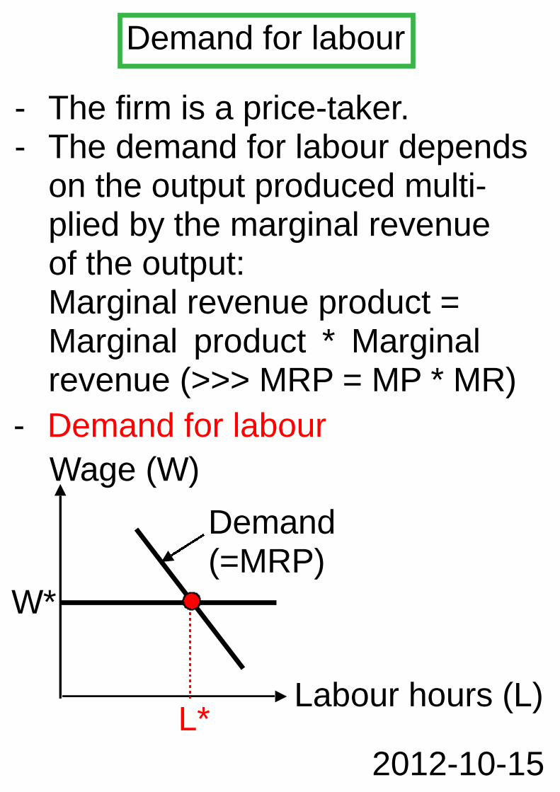
Demand for labour

- The firm is a price-taker.- The demand for labour depends

on the output produced multi-plied by the marginal revenueof the output:Marginal revenue product =Marginal product * Marginalrevenue (>>> MRP = MP * MR)

- Demand for labour

Wage (W)

Labour hours (L)

W*

Demand(=MRP)

L*

2012-10-15

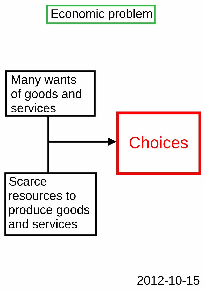
Economic problem

2012-10-15

Many wantsof goods andservices

Scarceresources toproduce goodsand services

Choices

- 2 consumers, A and B- 2 goods, X and Y- Combination of 2 indifference

curve maps of A and B

A

Contract curve:Efficient outcomes

Edgeworth box

B

Good X

Good X

2012-10-15

Elasticities

2012-10-15

Price elasticityof demand

Cross-price elas-ticity of demand

Income elasticityof demand

Price elasticityof supply

% change in qd% change in price

(result in absolute values)

% change in qd of good X% change in price of good Y

=

=

% change in qd% change in income

=% change in quantity supplied

% change in price

=

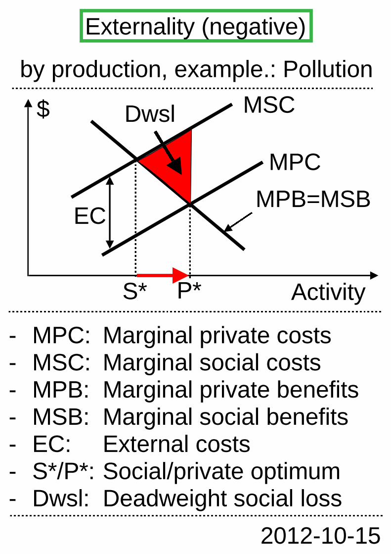
by production, example.: Pollution

- MPC: Marginal private costs- MSC: Marginal social costs- MPB: Marginal private benefits- MSB: Marginal social benefits- EC: External costs- S*/P*: Social/private optimum- Dwsl: Deadweight social loss

Dwsl

Externality (negative)

Activity

MSC

MPC

MPB=MSBEC

S* P*

2012-10-15

$

by consumption, ex.: Vaccinations

- MPC: Marginal private costs- MSC: Marginal social costs- MPB: Marginal private benefits- MSB: Marginal social benefits- EB: External benefits- S*/P*: Social/private optimum- Pwfg: Potential welfare gain

Pwfg

Externality (positive)

Activity

MPC=MSC

MSB

EB

S*P*

2012-10-15

MPB

$

A competitive firm is a price-taker.It chooses Q to maximize profit orminimize loss. Normal profits arepart of AC. Long-run equilibrium?

Competitive firm

Q

Firm and market

$

Market

MC

Q

$

D

S

AC

P=AR

2012-10-15

P

World P

Domestic D

2012-10-15

Domestic S

Domestic P

P

Q

Imports

Producer surplus

Tariff revenues

Welfare losses

Consumer surplus

Effects of an import tariff:

Import tariff (effects)

2012-10-15

% change in quantity demanded% change in income

=

Ie > 0

Normal good

Ie < 0

Inferior good

Income

qd

Income

qd

Income elasticity of demand

Income tax

Proportional tax Progressive tax

Tax rate

Income

AT=MT

Tax rate

Income

AT

MT

Total tax risesin proportionto income.

Total tax risesmore than pro-portional to in-come.

2012-10-15

$

Q

2012-10-15

10

105

From average to marginal revenue:- AR = 10 - Q- MR relates to changes in TR,

therefore, a bit of calculus:-- TR = AR * Q = 10Q - Q2

-- MR = (TR)' = 10 - 2Q

MR

AR

Marginal and average revenue

P

Q

Supply

2012-10-15

10

104

2

8

Demand

- Demand (Q) = 10 - PSupply (Q) = P - 2

- At equilibrium:Demand = Supply; therefore:10 - P = P - 2P = 6 and Q = 4

6

Equi-librium

Market equilibrium

Competition

$

Market structure (demand)

Monopoly

Oligopoly Monopolistic competition

Q

$

Q

$

Q

$

Q

MR

D=AR=MR D=AR

D1=AR1

2012-10-15

MR1

D2=AR2

MR2

D=AR

MR

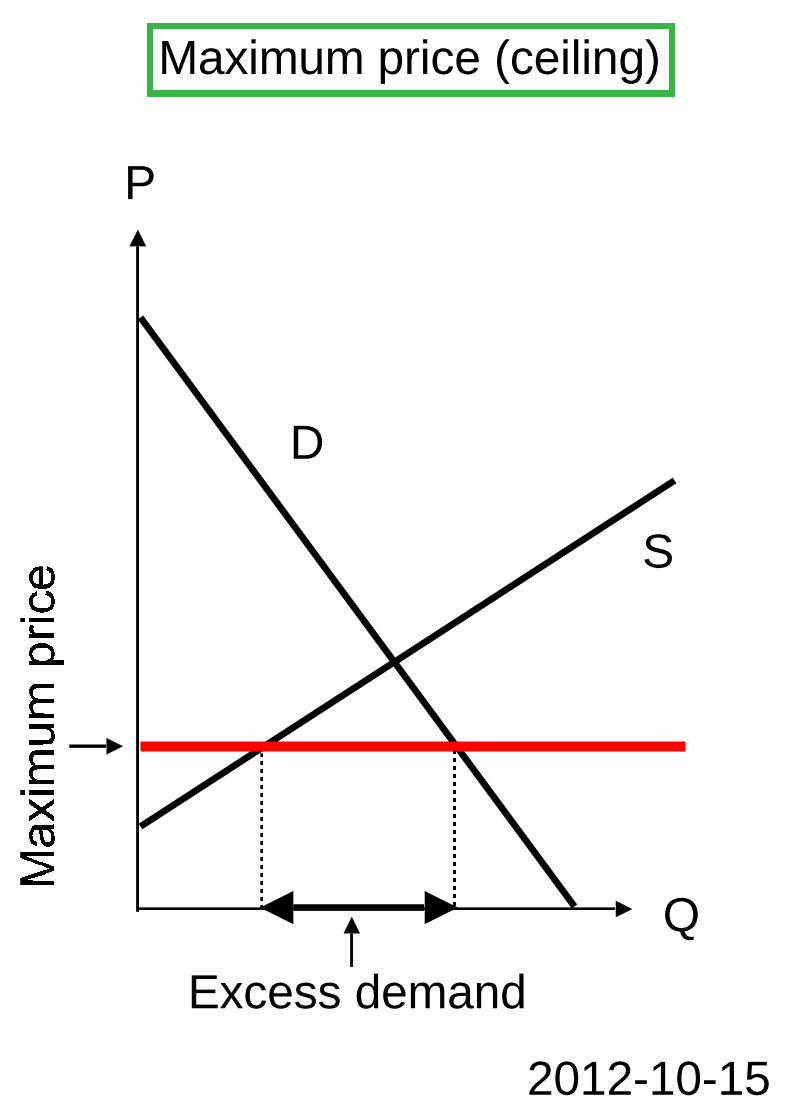
P

Q

S

D

2012-10-15

Excess demand

Maximum price (ceiling)

P

Q

SD

Minimum price (floor)

2012-10-15

Excess supply

A minimum wage causesunemployment (U),...

Minimumwage

Minimum wage

1)

2)

1)

... except when labourdemand increases.

Q L

2012-10-15

LD

LSU

Minimumwage

Q LLD 1

LSLD 2

Due to cost advantages (fallingAC/economies of scale) naturalmonopolies have a strong marketposition. Example: A firm investingin infrastructure (high fixed cost)

AC

P*

Natural monopoly

D=P=AR

$

QMR

MCAC

Supernormal profit

2012-10-15

2012-10-15

Pareto efficient inefficient

$ person B

$ person A

It is impossible to make one personbetter off without making anotherone worse off.

Example: Distribution of wealthbetween 2 persons

$ person B

$ person A

FrontierFrontier

Pareto efficiency

$

Q

D=P=AR

2012-10-15

Q

$

Pro

fit

A

D=P=AR

MRMR

MC =ACMC=AC

BP

rofit

Price discrimination

Segment B Segment A

Price in segment A

Price in segment B

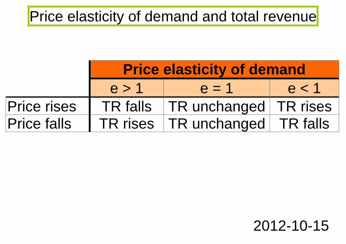
Price elasticity of demand and total revenue

Price elasticity of demand

e > 1 e = 1 e < 1Price rises TR falls TR unchanged TR risesPrice falls TR rises TR unchanged TR falls

2012-10-15

2012-10-15

1) e and D curve

4) e = 13) e=

2) e = 0P

Q

QQ

P

Q

P

Q

P

Q

Pe=

e=0

e=1

DD

D

D

83

3

8

Price elasticity of demand

2012-10-15

1) Se > 1

4) SR/LR S3) Se = 1

2) Se < 1P

Q

QQ

P

Q

P

Q

P

Q

P

LR SS 3

SS

S 2

S 1

SR S

Price elasticity of supply

P

Q

Producer surplus

S

D

Producer surplus

2012-10-15

Q good X

2012-10-15

Q good Y

PPF

1

2

Characteristics:- Concave shape of PPF:

Opportunity costs are risingwhen substituting more and moreX for Y.

- Points on the PPF are efficient.Other points:

inefficientunattainable

12

Production possibility frontier

Profit and loss (rules)

Marginal condition:

MC = MR

Average condition:

Maximum profit: AC < AR

Minimum loss: AC > AR

Normal profit: AC = AR

2012-10-15

$

Q

D=P=AR

2012-10-15

MR

AC

MC

AC

P

Find point MC = MR

Set price > MC = MR

Profit = (P - AC) * Q

Profit maximizationby a monopolist in 3 steps:

Q

Profit maximization by a monopolist

Long-run average cost

Q

Returns to scale

2012-10-15

1 Increasing returns to scale(= economies of scale)

2 Constant returns to scale3 Decreasing returns to scale

(= diseconomies of scale)

321

P

Q

S 2

D

Subsidies

2012-10-15

Subsidy

S 1

P 2

P 1

Q 1 Q 2

By a per-unit subsidy, price isdecreased and quantity is in-creased. In this case both sellersand buyers profit from subsidies atthe cost of taxpayers.

P

Q

Original S

2012-10-15

1

2

1

2

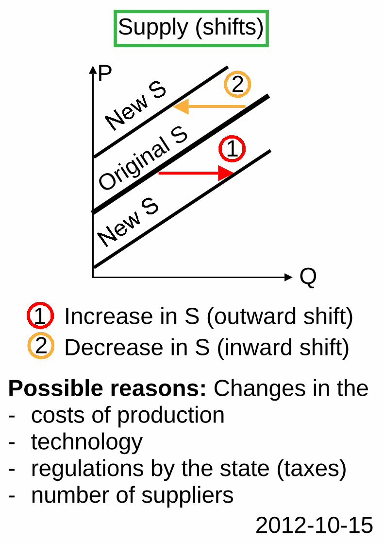
Increase in S (outward shift)

Decrease in S (inward shift)

Possible reasons: Changes in the- costs of production- technology- regulations by the state (taxes)- number of suppliers

Supply (shifts)

P

Q

Supply

2012-10-15

10

10

6

4

- Supply refers to the curve anddisplays the relationship betweenprices and quantities supplied.

- Quantity supplied refers to apoint on the curve.Example: If P = 6, then Q = 4;4 is the quantity supplied.

8

2

Supply and quantity supplied

P

Q

S 1

D

2012-10-15

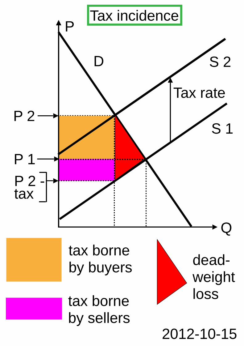
Tax rate

S 2

P 1

P 2

P 2 -tax

tax borneby buyers

tax borneby sellers

dead-weightloss

Tax incidence

Total utility

Utility

Q

Marginal utility

TU

Q

Law ofdiminish-ing MU

MU

Consumption equilibrium:

MU good AP good A

MU good BP good B=

2012-10-15