Michigan Technological University - MTRImtri.org/geoasset/media/doc/deliverable_Deliverable...

Deliverable 6-A: Cost benefit analysis of a proactive geotechnical asset management system using remote

sensing

Rudiger Escobar Wolf, El Hachemi Bouali, Thomas Oommen, Colin Brooks, and Stanley J. Vitton

Michigan Technological University

USDOT Cooperative Agreement No. RITARS-14-H-MTU Due on: June 15, 2015

Principal Investigator: Dr. Thomas Oommen, Assistant Professor Department of Geological and Mining Engineering and Sciences Michigan Technological University 1400 Townsend Drive Houghton, MI 49931 (906) 487-2045 [email protected] Program Manager: Caesar Singh, P.E. Director, University Grants Program/Program Manager OST-Office of the Assistant Secretary for Research and Technology U.S. Dept. of Transportation 1200 New Jersey Avenue, SE, E35-336 Washington, DC 20590 (202) 366-3252 [email protected]

mailto:[email protected]

Deliverable 6-A RITARS-14-H-MTU 1

TABLE OF CONTENTS Executive summary 3 1. The cost and benefit analysis framework 4 2. Estimating costs of different technologies and platforms 6 2.1 Defining unitary costs 6 2.2 Satellite based InSAR costs 7 2.2.1 Building in-house InSAR analysis capacities 7 2.2.2 Outsourcing the InSAR analysis 11 2.3 Aerial LiDAR costs 11 2.3.1 Building in-house capacities for aerial LiDAR analysis 11 2.3.2 Outsourcing the aerial LiDAR analysis service 12 2.4 Mobile LiDAR costs 14 2.4.1 Building in-house mobile LiDAR expertise 14 2.4.2 Outsourcing the mobile LiDAR analysis service 16 2.5 Terrestrial LiDAR costs 17 2.5.1 Building in-house terrestrial LiDAR expertise 17 2.5.2 Outsourcing the terrestrial LiDAR service 19 2.6 UAV SFM photogrammetry costs 19 2.6.1 Building in-house UAV SFM photogrammetry expertise 19 2.6.2 Outsourcing the UAV SFM photogrammetry service 23 2.7 Terrestrial SFM photogrammetry costs 24 2.7.1 Building in-house terrestrial SFM photogrammetry expertise 24 2.7.2 Outsourcing the terrestrial SFM photogrammetry service 24 2.8 Mobile SFM photogrammetry costs 25 2.8.1 Building in-house mobile SFM photogrammetry expertise 25 2.8.2 Outsourcing the mobile SFM photogrammetry service 26 3. Benefits from each technology and comparison with their costs 26 3.1 Defining information goals and expected performance in the context of GAM 26 3.2 Evaluation of information content and benefits from each remote sensing method 30 3.2.1 Point location and surface displacement accuracy 30 3.2.2 Point density 33 3.3 Synthesis of costs and benefits 36 4. Conclusions 38 5. References

39


GLOSSARY OF TERMS ALOS Advanced Land Observing Satellite

AASHTO American Association of State Highway and Transportation Officials

COSMO-SkyMed Constellation of small Satellites for the Mediterranean basin Observation

DEM Digital Elevation Model

DSLR Digital single-lens reflex

DSS Decision Support System

ENVISAT Environmental Satellite

ERS European Remote Sensing Satellite

FAA Federal Aviation Administration

GAM Geotechnical Asset Management

GB Giga-byte

GNSS Global Navigation Satellite System

GPS Global Positioning System

InSAR Interferometric Synthetic Aperture Radar

LiDAR Light Detection and Ranging

Meteor-3M Russian polar orbiting satellites

PALSAR Phased Array type L-band Synthetic Aperture Radar

RADARSAT-1 and 2 Radar Satellite 1 and 2

RAM Random access memory

RMSE Root mean squared error

RTK Real-time kinematic

Sentinel-1A and 1B European Space Agency radar imaging satellites

SEOSAR/Paz Satélite Español de Observación SAR (Spanish SAR observation satellite)

SFM Structure from Motion

TerraSAR-X German radar earth observation satellite

UAV Unmanned aerial vehicle

USDOT/OST-R US Department of Transportation, through the Office of the Assistant

Secretary for Research and Technology

USGS Unites States Geological Survey

VTOL Vertical takeoff and landing


EXECUTIVE SUMMARY: DELIVERABLE 6-A

Overall Goal of this Deliverable: To present a summary of the costs and benefits of applying

three technologies to monitor geotechnical assets: Satellite base Interferometric Synthetic

Aperture Radar (InSAR), Light Detection and Ranging (LiDAR), and Structure from Motion

(SFM) Photogrammetry. Costs are estimated from different sources, including costs reported in

the literature and costs directly assessed as part of the project’s data collection and analysis.

Benefits will be assessed in the context of the value that can be assigned to the information

content produced by the different methods. Specifically, the information content is defined in

reference to geotechnical assets surface displacement, and the relative value is judged in terms of

its accuracy and data point density. Different scenarios that consider various in-house versus

outsourcing of service, and higher versus lower precision data acquisition setups are considered

and discussed. Comparisons between the different scenarios and their impact on cost, accuracy

and data point density are included at the end.

Acknowledgements

This work is supported by the US Department of Transportation, through the Office of the

Assistant Secretary for Research and Technology (USDOT OST-R). The views, opinions,

findings, and conclusions reflected in this paper are the responsibility of the authors only and do

not represent the official policy or position of the USDOT OST-R, or any state or other entity.

Additional information regarding this project can be found at www.mtri.org/geoasset

http://www.mtri.org/geoasset


1. The cost and benefit analysis framework

The adoption of new technologies, like the remote sensing methods proposed for geotechnical

asset management and monitoring, requires the evaluation of the potential benefits they offer,

versus the potential costs of implementing them (Ye et al. 2014). The assessment of the potential

costs and benefits of the new technology is crucial to decide whether it is worth adopting it

compared with other alternatives, including monitoring methods currently in place, or in some

cases no monitoring at all. We will use the framework of costs and benefits for similar

technologies and applications laid out in the literature, particularly for LiDAR applications, e. g.

Ye et al. (2011, 2014), Vincent and Ecker (2010), Olsen et al. (2013), Chang et al. (2014), and

Williams et al. (2013).

Commonly the term “cost-benefit analysis” is used for assessing the net societal benefit of large

projects that have a direct impact on the broader public, and is therefore considered a public

policy assessment tool (e. g. Boardman et al., 2006; Zerbe and Bellas, 2006). The assessment of

the costs and benefits of remote sensing technologies for geotechnical asset management has to

be framed within the wider context of transportation asset management. In such a context, the

monitoring technology only corresponds to a small component of the whole asset management

system. Therefore, our goal for this report is rather modest, we only aim to provide a discussion

of the relative costs of the technologies and compare some of their potential benefits, within the

context of their use for geotechnical asset management.

In the case of remote sensing technologies applied to monitor the state of geotechnical assets, the

main product obtained from their use is the information on the asset's conditions, e. g. if a slope

shows movement. It is the value of that information what determines the potential benefits of the

technology. The value of this information is dependent on the use that will be given to it. In the

particular case of geotechnical asset management, the information's value depends on the use of

the information for decision making related to the assets maintenance, repair or replacement, as

part of a geotechnical asset management system (Sanford-Bernhardt et al., 2003; Vessely, 2013;

Stanley, 2011). If there is an adequate decision making platform where the information generated

by remote sensing techniques is a critical input the value of that information will be high,

resulting in a significant benefit, otherwise the information has no value.


To compare the costs with the benefits, and assess whether the benefits outweighs the costs, it is

necessary to reduce both to a common metric, usually in terms of economic value through the

monetarization (i. e. assigning a dollar value) of each item that will contribute to the potential

cost and benefits (Boardman et al., 2006; Zerbe and Bellas, 2006). In our case, rather than

monetary values for particular cases of the technological applications, we will give a range of

examples and broad estimations of costs, and a qualitative description of benefits from using the

proposed remote sensing technologies. Two main types of scenarios regarding costs will be

presented, the cost of developing “in-house” capabilities to use the technology, and the cost of

contracting a service provider who can apply the technology and will deliver a final product,

similar to what would be obtained if the technology capacity was built “in-house”.

The benefits will be discussed in the context of the value of information generated by each

specific technology. The main product of the remote sensing technologies explored in this project

is the detection and measurement of changes in the surface (displacements, deformation or

movement in general) of the assets being monitored (e. g. cut slopes, retaining walls, etc.).

Tracking such changes through time and considering them in the relevant geotechnical context

(e. g. what are the slope stability implications for a movement of a given magnitude measured on

a cut slope) is the basis for using the information in a decision support system, which is also

currently in development as part of the project. A synthesis of the cost and benefit will be

presented, comparing costs and benefits between the different technologies, but keeping in sight

the differences in the outputs and potential applications of each technology.

Given the large range of possible applications, the variability in costs depending on such

applications, and the even more significant complexity of the potential benefits that could be

attached to the information produced by the remote sensing techniques, we will also present and

discuss the uncertainties in our analysis and the relevant limitations of the available information.

Part of this uncertainty is related to the state of development of other components in this project,

including the testing and validation of the remote sensing methods, and the development of a

decision support system, in which the information would actually be an input. We will make

some assumptions about these components, but an update may be necessary after the

corresponding project products are completed.


2. Estimating costs of different technologies and platforms

2.1 Defining unitary costs

When possible, the general cost estimation and discussion will be based on the assumption of

two scenarios: first we consider an “in-house” capacity building scenario, in which all the

hardware and “know-how” is acquired by the user of the technology (e. g. a State Transportation

Agency). Second, we consider the outsourcing scenario, in which the costs correspond are those

of contracting a service provider, who applies the technology and provides the user with a final

product (e. g. surface displacement measurements). For the “in-house” scenario we will consider

the initial investment costs, as well as long term operation costs. The outsourcing costs are

compiled from market value costs reported in the literature and by the project partners.

The in-house scenarios includes initial costs related to an initial investment, necessary to buy the

hardware and software, as well as procuring the training for operators and analysts that will be

necessary to apply the technology, and the long term, sustained cost for the operation or recurrent

use of the technology. The long term cost will be discussed on an annualized basis, and no

discount analysis of present value will be performed, but the impact of long term payoff of the

initial investment will be discussed in section 3, when integrating cost and benefit considerations

(e. g Ye et al. 2014; Chang et al. 2014).

The outsourcing scenario only considers the recurrent use of the contractor's service. Whether in-

house or outsourcing is a better alternative will depend on several factors, but usually the in-

house capacity will be justified by a higher demand for the technology, i. e. more frequent or

extensive use, while the outsourcing tends to be more cost effective for lower work volumes.

According to this reasoning, agencies dealing with extensive geotechnical assets, distributed over

large areas of very active (e. g. relatively steep and often unstable) terrain may find the in-house

capacity building more cost efficient, than agencies dealing with a smaller volume of such assets

and their corresponding workload.

Some of the technologies and platforms may not be available in both in-house and outsourcing

scenarios. The case of aerial LiDAR surveying is presented in section 2.3, discussing the reasons

that make developing an in-house capacity unfeasible for most cases in section 2.3.1, and


therefore only a quick overview of that case is presented. The opposite happens in the case of

structure from motion (SFM) photogrammetry discussed in section 2.6; in that case only the in-

house scenario is considered (section 2.6.1), given the current state of development of the

technique and the corresponding lack of commercial service providers (section 2.6.2). Because

the fundamental differences in the methods, the cost of traditional photogrammetric services are

unlikely to be representative of market costs for SFM photogrammetry, and therefore are not

considered here as a proxy for the UAV based platform.

Cost estimates are presented as either total costs per project (or site) location, costs per linear

transportation corridor unit (dollars per mile) or costs per day of operation, depending what units

are more relevant to the specific application. Long term costs included in the in-house scenarios,

like the initial investment in equipment, are distributed over time on an annual basis.

2.2 Satellite based InSAR costs

2.2.1 Building in-house InSAR analysis capacities

Initial investment cost to build in-house capacities to use InSAR as a monitoring tool include

buying the software and hardware necessary for data analysis. The main hardware consists of

computer equipment with enough processing power to operate the software, and electronic

storage volume for hosting the data files. Computer hardware requirements vary depending on

the software used, but high power commercial desktop models are usually sufficient e. g. a

desktop computer with an Intel Core i7 series processors, 16 GB of RAM and 1 to 2 TB of

storage space. Such hardware has a cost ranging between $ 1,500 and $ 2,500.

Software license costs vary over a large range, depending on the type and brand of software

used, from $ 8,000 up to $ 65,000. We used the commercial Sarmap software (Sarmap, 2009),

which provides capabilities to process single interferograms from pairs of satellite images, and

persistent scatterer points from image stacks (for more details see Deliverable 2-A: report

“Candidate remote sensing techniques for the different transportation environments,

requirements, platforms, and optimal data fusion methods for accessing the state of geotechnical

assets”). Sarmap falls in the lower end of software prices and delivers most of the products

considered in this project for InSAR.


Sustained costs include the computer time cost, and the analyst time costs. If a computer is

bought for the sole purpose of InSAR data analysis, as a dedicated resource, no further

computing time cost considerations are necessary, but the cost of maintaining the equipment, and

most significant, the cost of hosting the data on server, etc., may represent and additional cost, as

part of the agency’s IT operations. We estimate an IT cost for storage and backup of ~ 20 TB of

data. Using current hard drive storage costs from commercial, including space for multiple

periodic backups, we estimate an annual cost of $ 0.2 per GB, which gives a total cost of $ 4,000

per year.

Dedicated analyst time cost will vary depending on how much the analyst has to interact with the

software (e, g, how complex and challenging the data set is) and the amount of data that need to

be processed. The analyst time also includes the time spent searching the datasets to be used, in

image catalogues. Processing a single stack of several tens of images can take several hours to

more than a week of continuous processing for the software, but will only require a few hours of

work by the analyst for preparing the input, starting the processing sequence of the software, and

evaluating the software output at the end.

A conservative estimate for the analyst time devoted to a single site analysis, using a large stack

of images (e. g. 40 images), is 8 hours on average. Considering a cost of $40 per hour for a

trained analyst, we get a rough estimate of $320 per site analyzed. This can vary significantly,

increasing if the terrain is challenging and further interaction from the analyst is required. It is

difficult to estimate the number of sites, or image stacks that would have to be analyzed in a year,

but it could be between a low of 10 sites and a high of 50, which would translate to annual labor

costs between $ 3,200 and $ 16,000.

Data acquisition costs depends on the type of satellite imagery being acquired. Cost for

commercial applications imagery range from free available images for Sentinel 1B, to > $ 7,000

for RADARSAT-2 per image, but usually fall on the lower end of the cost range, e. g. hundreds

of dollars per image (see table 1). It becomes obvious that the imagery cost can be significant,

especially when stacking techniques that use tens of images are applied. Using a high average

estimate of $ 1,000 per image, a single interferogram analysis using an image pair would imply a


$ 2,000 cost, and an image stacking analysis, like that performed for persistent scatterers, using

20 to 40 images would amount to $ 20,000 to $ 40,000 in costs. The number of images used

depends on the extension of geotechnical assets that need to be monitored, the ground location of

the image footprint, and the image size (see figure 1, for an example). The tendency in the near

future for agencies that produce and deliver such images, is to reduce the cost or even provide

them for free, like in the case of the Sentinel 1b imagery, but this consideration does not apply to

historical data necessarily. Assuming that each image footprint contains 100 miles of

transportation corridor, and that a transportation agency needs to analyze 100 to 1,000 miles

every year, the agency would have to analyze 1 to 10 locations, costing a total of between $

20,000 and $ 200,000.

Table 1. InSAR satellite images characteristics.

Satellite Mission Timespan

Revisit Period (days)

Ground Resolution

(meters) Price Per Image (US Dollars)**

ERS-1 1991 - 2000 35 25 $212 - $354

ERS-2 1995 - 2011 35 25 $212 - $354

RADARSAT-1 1995 - 2013 24 10-100 $3,047 - $3809

ENVISAT 2002 - 2013 35 25-150 $354 - $591

ALOS PALSAR 2006 - 2011 46 7-100 $42 - $709

RADARSAT-2 2007 - 24 3-100 $3,047 - $7,110

COSMO-SkyMed 2007 - 16 1-100 $680 - $2,268

TerraSAR-X 2007 - 11 1-16 $875 - $7,972

Meteor-3M 2009 - 3 400-1,000 $30/$40 - ?

ALOS PALSAR-2 2014 - 14 1-100 $1,257 - $4,191

Sentinel-1A 2014 - 12 4-80 Free of cost

SEOSAR/Paz 2015 - 11 1-15 Will be publically available

Sentinal-1B 2016 - 6 4-80 Will be publically available

COSMO-SkyMed 2nd Generation

2016 - 1.5-10 1-35 Will be publically available

**US Dollar exchange rates (January 2015). NA = not available for commercial or educational use. Prices and data

availability listed for users in the United States.


Figure 1. Example of different InSAR images area coverage over Fairbanks, Alaska.

From the above discussion we see that the cost of commercial InSAR applications developed

“in-house” will be dominated by data acquisition costs, especially for longer time trend analysis

like those performed with stacking techniques.

Table 2. Summary of costs for in-house InSAR analysis capacities

Item Cost estimate

Low High

Computer hardware 1,500 2,500 Software 8,000 65,000 Annual data storage 4,000 4,000 Annual analyst labor 3,200 16,000 InSAR images 20,000 200,000 Total 36,700 287,500

RADARSAT-1 (Descending)

ERS-1 & ERS-2

ALOS PALSAR

RADARSAT-1 (Ascending)


2.2.2 Outsourcing the InSAR analysis

Commercial service providers for analyzing InSAR imagery are also available. The costs of such

services will also depend on the requested products and the availability of satellite imagery. As a

comparison within the aims of the project, a commercial InSAR analysis service provider

performed a similar analysis to that done with our “in-house” developed capacities, and although

the outputs were not entirely comparable, as discussed in sections 3 and 4, the costs can broadly

be compared as an indicator of similar services. For a single site and using the same imagery (e.

g. 90 images acquired at no cost for research purposes) as our “in-house” test, the reported costs

by the commercial provider ranged between $ 20,000 and $ 50,000. The addition of the imagery

cost could increase the final price of the commercial service, for cases outside of the research

test. As with the scenario described in section 2.2.1, we assume that between 1 and 10 locations,

corresponding to between 100 and 1,000 miles, need to be analyzed, which would add to an

annual costs between $ 20,000 and $ 250,000.

Table 3. Summary of costs for outsourcing the InSAR analysis

Item Cost estimate

Low High

Outsourcing InSAR analysis 20,000 250,000 Total 20,000 250,000

2.3 Aerial LiDAR costs

2.3.1 Building in-house capacities for aerial LiDAR analysis

Developing in-house aerial LiDAR capabilities is usually very expensive and will not be a

feasible option for the majority of users, except the largest agencies, which may have to deal

with extensive geotechnical asset inventories and challenging conditions (e. g. steep and

geologically active terrain). The use of aircraft equipped with special adaptations to carry the

LiDAR instruments, and a high accuracy navigation system to geolocate the LiDAR data, makes

the use of non-dedicated (e. g. rented) aircraft complicated. The high power LiDAR instruments

used for aerial data acquisition are also more expensive than the terrestrial LiDAR scanners

discussed in the next section (Shan and Toth, 2009), and the expertise involved in operating such


aircraft and instruments leads to most or all of the data acquisition steps being outsourced to

specialized commercial providers (Chang et al. 2014).

Vincent and Ecker (2010) present a detailed aerial LiDAR cost estimate of $ 8321 per mile of

corridor, for a transportation corridor survey in Missouri, when all the costs for the operation of

the aircraft and other logistics are taken into account (see also discussion of this case in Chang et

al. 2014). This estimation is however for a very high point density and accuracy survey,

comparable to the point densities and accuracies that can be obtained by mobile and static

LiDAR collects. We assume that most agencies that end up using aerial LiDAR data will

outsource the data collection and analysis to a commercial service provider, and the costs are

therefore expected to be similar.

Table 4*. Summary of costs for in-house capacities for aerial LiDAR analysis

Item Cost estimate

Low High

Total (non-itemized) cost 25,200 541,000 Total 25,200 541,000

*Taking the same total values as in table 5.

2.3.2 Outsourcing the aerial LiDAR analysis service

The amount that the aerial LiDAR service providers charge for their services depends on the

specifications defined by the user (e. g. ground point density and accuracy), the data processing

level at delivery (e. g. raw point clouds, “last return” classified point clouds, DEMs, etc.), the

complexity and level of difficulty of the terrain (e. g. relief, slope, forest cover, etc.), site

locations, (e. g. remoteness), and size of the survey job (e. g. larger areas have a smaller unit area

cost). Costs are usually quoted per covered area unit, for a given “level of quality”.

A study for the USGS National Data Elevation Assessment from 2012 reports cost for large area

(> 5000 sq. mi) ranging from $ 90 to $ 521 per square mile, depending primarily on the “quality

level”, which defined in terms of data point density, nominal pulse spacing, vertical RMSE, and

equivalent contour accuracy (Dewberry, 2012). Aerial LiDAR costs for the State of Michigan

(for 2013) range from $ 100 per square mile, for surveys of areas larger than 5,000 square miles,


to ~ $ 250 per square mile, for survey areas smaller than 100 square miles (State Of Michigan

Center For Shared Solutions, 2013). Specifying higher or lower quality levels for the data can

increase the cost by more than a factor of 2. These values are comparable to the aerial LiDAR

costs of $ 335 per square mile estimated for Wisconsin in 2014 (McDougal, 2014) and $ 344 per

mile, estimated for Vermont in 2015 (Vermont Center for Geographic Information, 2015), in both

cases a standard USGS “quality level” 2 was specified.

Because in this project we assume that the primary targets for the LiDAR survey are

transportation corridors, it is more meaningful to give the costs as unit length costs (i. e. dollars

per mile of corridor), rather than unit area costs (dollars per square mile of terrain). Assuming a

wide enough buffer zone to include the transportation corridor and all relevant geotechnical

assets (e. g. natural and cut slopes), and considering the limitation of the minimum altitude above

the terrain that the aircraft can fly and the footprint size of the LiDAR scans, one can convert

from the unit area cost to a unit length cost. Additionally, the limitations of the flight path, which

may not be able to follow a highly sinuous transportation corridor layout, also has to be

considered. For a swath width of half a mile and using the areal costs discussed in this section we

get linear unit costs in the range of $ 45 to $ 250 per mile of surveyed corridor. However, the

requirement of a minimum survey area, sometimes imposed by surveying companies, may drive

the actual cost per surveyed mile up.

The length of the transportation corridors that need to be surveyed will depend on the type of

asset monitoring. Agencies with extensive geotechnical assets in very active terrain, and which

require close monitoring (e. g. in areas with rugged and steep terrain) may want to survey

thousands of miles of their transportation network. While agencies with less complex terrain and

more stable or simpler asset inventories may focus on shorter stretches of their transportation

network. Assuming that the total corridor length to be surveyed in any given year is somewhere

between 100 and 1,000 miles, the annual cost would be between $ 25,000 and $ 521,000.

Once the data have been delivered to the user (e. g. a transportation agency), a data archiving and

management process is necessary, and that basically involves planning for data storage. Data

storage space could potentially be much larger compared to InSAR, if a similar area (or corridor

length) is being surveyed with aerial LiDAR. Storage space requirements of up to 10 GB per


mile could be expected. Assuming an annual cost of $ 0.2 per GB and an annual transportation

corridor surveying length of 100 to 1,000 miles, a total annual cost between $ 200 and $ 2,000

has to be considered.

Table 5. Summary of costs for outsourcing the aerial LiDAR analysis service

Item Cost estimate

Low High

Outsourcing LiDAR analysis 25,000 521,00 Annual data storage 200 20,000 Total 25,200 541,000

2.4 Mobile LiDAR costs

2.4.1 Building in-house mobile LiDAR expertise

Detailed cost, and cost-benefit analyses for developing in-house mobile LiDAR capabilities are

presented and discussed by Vincent and Ecker (2010), Yen et al. (2011 and 2014), and Chang et

al. (2014). These cases assume that cost of initial investment in equipment, can be distributed

over a long time period (up to 6 years).

Initial investment to build in-house capacities include the investment in LiDAR instruments for

data acquisition, as well as computer hardware and software for data processing and analysis.

Commercially available LiDAR equipment costs vary between $ 5,000 and $200,000 at 2011

prices (Yen et al. 2011). Initial investment in software include the license for the data analysis

software, which can range from $ 500 to $ 80,000, depending on the capabilities and

functionality (Yen et al. 2011). For our project we used software on the lower end of the pricing

scale ($ 3,500), but had to resort to other in-house coding software (i. e. Matlab®) to do some of

the processing. Initial investment in hardware include computers for data processing and data

storage space, and we assume similar computer costs to those previously described for the

InSAR processing, i. e. between $ 1,500 and $ 2,500.

Although virtual storage space needs for the collected data would be expected to be larger than

for aerial LiDAR, given the higher point densities for achieved for mobile LiDAR collection, the

area covered by such surveys will typically be much smaller. Annual data storage costs reported


by Yen et al. (2014) seem exaggerated, at $ 7.3 per GB, as physical hard drives with periodical

backup functionality may be a much cheaper option. Using their estimate of 3 GB per mile of

data, the memory cost would amount to $ 21.9 per mile. If instead we use the annual cost of $ 0.2

per GB used for the InSAR data storage in section 2.2.1, we obtain an annual data storage cost of

$ 0.6 per mile of surveyed corridor. Assuming that transportation corridor lengths that will be

surveyed any given year are somewhere between 100 and 1000 miles, the annual cost of data

storage would amount to $ 60 to $ 600.

Data collection costs vary greatly depending on the type of data collected, and particularly the

required accuracy, which determines the requirement to establish ground control, etc. These costs

include the time of all the field personnel, vehicle and gasoline costs, and very importantly, the

cost of establishing accurate ground control, which may be much more costly than the LiDAR

data collection per se.

For data collections using high accuracy ground control Vincent and Ecker (2010) estimated a

cost of $ 9,933 per mile of corridor, while Yen et al. (2014) estimate costs between $ 385 and $

531 per mile of corridor, for data collects without external ground control (their options 4 and 6

on table 4). These values cover a similar range of costs compared to the aerial LiDAR costs

presented in section 2.3. The differences between the costs estimates by Vincent and Ecker

(2010) and those estimated by Yen et al. (2014), is in large part due to the high cost of

establishing ground control using traditional surveying methods in the first study. For surveyed

transportation corridor lengths of 100 to 1000 miles, the annual costs would be somewhere

between $ 38,500 and $ 531,000 for the type of survey described by Yen et al. (2014), and

somewhere between $ 993,300 and $ 9,933,000 for the type of survey described by Vincent and

Ecker (2010).

LiDAR data collected for monitoring surface displacement would be required to be highly

accurate, with errors not larger than a few centimeters. With the current technology this would

require processing methods that rely on precise ground control, shifting the costs to the upper

end of the range reported here. However, new technology, and particularly RTK GPS and INS


technology coupled to the LiDAR instruments, may allow users to rely less on ground control in

a near future (Olsen et al., 2013; Williams et al. 2013).

Data processing costs include an average of 2 hours of labor per GB of collected data, and taking

the estimate of 3 GB of data per mile, and a cost of $ 40 per hour for the technician doing the

analysis, the cost of processing the data would be $ 240 per mile. Surveying an annual corridor

length of 100 to 1,000 miles would cost somewhere between $ 24,000 and $ 240,000.

Table 6. Summary of costs for in-house mobile LiDAR expertise

Item Cost estimate

Low High

LiDAR instrument 5,000 200,000 Analysis software 500 80,000 Computer hardware 1,500 2,500 Annual data storage 60 600 Ground control surveying (rapid)1 38,500 531,000 Ground control surveying (high accuracy)1 993,300 9,933,000 Data processing labor 24,000 240,000 Total (with rapid control)1 69,560 1,054,100 Total (with high accuracy control)1 1,024,360 10,456,100

1Two sub-scenarios are considered here, depending on whether rapid or high accuracy ground control is used.

2.4.2 Outsourcing the mobile LiDAR analysis service

The range of costs given by Yen et al. (2014) for the outsourcing case is very similar to the in-

house option. Some of the cases presented by them are mixed cases, where some of data

acquisition and analysis process is outsourced, but other parts are done in-house, and would

require building such a capability by the user. Completely outsourcing the service resulted in a

cost of $ 476 per mile (their option 1 in table 4), and mixed options spanning a wider range of

costs, from $ 422 per mile for renting the LiDAR equipment and assuming the costs of the

survey (their option 3 in table 4), to $ 717 per mile for their “partial ownership” of the equipment

case (their option 7 in table 4). All these estimates correspond to data collection without accurate

external ground control. Much higher costs, similar to those presented by Vincent and Ecker

(2010) for the in-house case, would be expected if high accuracy external control had to be set

up, driving up costs to as much as 10,000 per mile. Annual costs for 100 to 1,000 miles of


surveyed transportation corridor would then fall between $ 42,200 and $ 717,000 for the lower

accuracy survey, and between $ 1,000,000 and $ 10,000,000 for the higher accuracy survey of

control points, but such high accuracy ground control surveys are never used for mobile LiDAR

surveys in practice.

Table 7. Summary of costs for outsourcing the mobile LiDAR analysis service

Item Cost estimate

Low High

Outsourcing mobile LiDAR service (rapid control) 42,200 717,000 Outsourcing mobile LiDAR service (high accuracy control) 1,000,200 10,000,000

2.5 Terrestrial LiDAR costs

2.5.1 Building in-house terrestrial LiDAR expertise

Terrestrial LiDAR collections are typically done for projects where high accuracy is necessary,

and the use of precise external ground control is required. We assume that this is the case for

both the in-house and the outsourced terrestrial cases discussed here. Vincent and Ecker (2010)

give an estimate cost of $ 29,258 per mile of terrestrial LiDAR survey. Given the high cost and

large data volumes produced by this method, it is usually not applied to large stretches of

transportation corridors, but rather focused on smaller areas of interest, like unstable slopes or

other deteriorating geotechnical assets. This is the use envisioned for the geotechnical asset

management in this project, and the discussion will follow that concept.

Figure 2. Riegl LMS-Z210ii instrument used to collect terrestrial LiDAR points at the field site in Nevada.


Using the unit cost estimates given by Vincent and Ecker (2010) in their table 8 (page 56) and

adjusting the times for a single work day, we get an estimate cost of $ 10,000 per day of

terrestrial LiDAR surveying, including setup of external control, and data processing and

analysis. Depending on the geotechnical asset size and the potential extension of the problem (e.

g. slope instability) it may take less or more than a day to survey it. The use of terrestrial LiDAR

may be reserved to the most critical cases, which require a more intensive monitoring, e. g.

slopes that show movement and which would have a large impact if they failed. The total number

of days that would be used for this kind of survey on a given year depend, as in previously

discussed cases, on the extension and size of the geotechnical asset inventory managed by each

agency, and the complexity and challenges of the terrain in which they are located. Assuming 10

to 100 days of survey data collection and processing that will be required each year for

monitoring critical assets, the total annual costs could be somewhere between $ 100,000 and

$ 1,000,000.

If the required ground control accuracy is less than the accuracy that would be obtained with

standard, high precision surveying instruments, a less accurate “rapid” method, based on a high

performance, hand held GPS receiver can be used (see section 2.6.1 for a detailed explanation).

The rapid version for georeferencing the ground control points has an estimated cost between

$ 400 and $ 800 per day of fieldwork, depending on the number and distribution of the control

points. When we substitute these values in the surveying corresponding budget item given by

Vincent and Ecker (2010) and recalculate the daily costs we obtain a cost value between $ 7,200

and $ 7,600 per day. Using the same figures of 10 to 100 days of data collection we obtain

annual costs of $ 72,000 and $ 760,000.

Additionally, data archiving and management needs to be considered. Taking the annual cost of $

0.2 per GB, and assuming a daily data collection volume of 100 GB, we estimate a cost of $ 20

per work day, and annual totals between $ 200 and $ 2,000, assuming 10 to 100 days of survey

data collection and processing.


Table 8. Summary of costs for in-house terrestrial LiDAR expertise

Item Cost estimate

Low High

LiDAR data collection and analysis (high accuracy control)1 100,000 1,000,000 LiDAR data collection and analysis (rapid control)1 72,000 760,000 Annual data storage 200 2,000 Total (with high accuracy control)1 100,200 1,002,000 Total (with rapid control)1 72,200 760,000


2.5.2 Outsourcing the terrestrial LiDAR service

The cost of contracting commercial service providers will depend on the characteristics of the

project, but are expected to fall within the range of costs outlined for the in-house scenarios from

section 2.5.1 (Chang et al. 2014), i. e. $ 10,000 per day of data collection and analysis, and

similar ($ 100,000 to $ 1,000,000) annual costs for a 10 to 100 days per year of survey data

collection and processing scenario.

Table 9. Summary of costs for outsourcing the terrestrial LiDAR service

Item Cost estimate

Low High

Outsourcing terrestrial LiDAR service 100,200 1,002,000 Total 100,200 1,002,000

*Taking the same total values as in table 8. Only the high accuracy case is shown.

2.6 UAV SFM photogrammetry costs

2.6.1 Building in-house UAV SFM photogrammetry expertise

Our cost estimates are based on past projects experience (e. g. Brooks et al. 2013) and our

experience with the current project. Initial investment in hardware includes the cost of the UAV,

the photographic camera and lenses, and other peripheral equipment (e. g. intervalometer for

automatic picture acquisition). UAVs can be of several different types, but here we will consider

two types: multi-rotorcraft and fixed wing. Multi-rotorcraft UAVs allow for greater flexibility in

deployment due to the VTOL capabilities, e. g. they don’t need much space for takeoff or

landing, but can have lower payload capacities, and usually cannot cover as large areas as the


fixed wing UAVs. Which type is more appropriate for a given task will depend on how these

characteristics influence the UAV performance for the task.

UAVs vary in cost from about $ 500 to more than $ 10,000. This project has taken advantage of

the capabilities that can be provided by UAVs in the $800 to $10,000 range. Cost differences

reflect the size and complexity of the UAVs, and therefore their functionalities and capabilities.

Larger and more expensive UAVs can carry heavier payloads and stay longer on the air, but may

be less maneuverable. We have used a 6 rotor (hexacopter) UAV produced by Bergen R/C

Helicopters. The cost of this UAV, fully equipped with batteries and navigation hardware and

software is $ 5,400.

Figure 3. Hexacopter UAV used for SFM photogrammetry in the project.

The camera used was a Nikon D800 DSLR camera, with a 36 megapixel sensor, a 50 mm f/1.4

lens and a built in GPS and intevalometer. The total cost of the camera and accessories was $

3,600. Data storage requirements of point cloud products will be comparable to those for

terrestrial LiDAR, but additional storage space is needed for the high resolution (e. g. 36

megapixel) photography. Total data volumes (photographs and cloud point products) may

amount to 250 GB collected per day. Using the annual cost of $ 0.2 per GB we have assumed in


previous calculations, would give a cost of $ 50 per day for data storage. Assuming 10 to 100

days of data collection in any given year, the annual cost for data storage would be between $

500 and $ 5,000. Analysis software costs range between $ 2,000 and $ 15,000, and for this

project we are using software (AgiSoft ® Photoscan) on the lower end of the price range.

Maintenance and operation costs for the UAV and camera system are expected to be on the order

of $ 710 per year, assuming a similar work load (~ 63 days for data collection and 21 days for

processing) as presented by Brooks et al. (2013). Following those assumptions, the annual

operation costs would amount to a total of $ 20,160 for data collection labor and $ 6,720 for data

processing. If instead we assume 10 to 100 days of data collection per year, as in previous

examples, the adjusted annual cost for data collection would be $ 32,000, and the annual cost for

data processing would amount to $ 10,667.

External ground control can be established in different ways for the UAV photogrammetry, and

at the moment this process is still subject to experimental testing as part of the project. We have

used a high performance hand-held Trimble GeoExplorer GNSS receiver to survey ground

control point locations. We only use the internal antenna and collect data for 10 to 20 minutes, to

get < 10 cm geolocation accuracies. Such rapid geolocation strategy reduces the time for

deployment of the groundcontrol targets, therefore reducing the costs involved in fieldwork, but

it also reduces the accuracy of the control points, impacting the overall quality of the data. A

more in depth discussion of that impact on the information value of data will be given in section

3. It is also possible to do a much higher accuracy survey of the control points, e. g. through

static differential GPS or total station surveying of the control points. Such high accuracy

methods would increase the costs by a large amount, similar to what happens in the case of

terrestrial LiDAR surveys presented in section 2.5.

Deploying and surveying the ground control points is usually the most labor intensive and time

consuming part of the fieldwork. The amount of work and time it can take to set up the ground

control points depends on the terrain conditions and the density or spacing between the points.

The density of control points should be as high as possible, but hiking on very rugged or steep

terrain will significantly limit the access in some cases, and even in easily accessible terrain,


practical time constraints will finally put a limit to the number of points that can be surveyed.

Since the targets for the proposed applications will be at, or near transportation corridors, the

access issue will usually not be a major concern. UAVs with RTK GPS capability, which have

become available in 2015, would reduce or eliminate the need for ground control points.

In our field tests the average spacing between control points has ranged from a few tens, to more

than a hundred meters. We estimate that on average it takes 1 hour of labor to deploy and survey

each control point, using the hand-held sub-meter accuracy GPS with occupation times of 10 to

20 minutes, described earlier. This would result in 10 to 20 work hours per mile, which would

cost $ 400 to $ 800. Higher accuracy surveying, using differential GPS or total station would

increase that cost to $ 1,000 to $ 2,000 dollars per mile. Alternatively, for a typical day of data

acquisition it would be necessary to deploy a similar number (10 to 20) of ground control points

resulting in a similar cost of $ 400 to $ 800 per day for the lower accuracy (hand-held GPS)

surveying type. Annual costs, considering 10 to 100 days of surveying for the data acquisition,

would amount to $ 4,000 to $ 80,000, a cost that would need to be added to the cost previously

considered in this section. The physical targets consist of plastic sheets with a distinct black and

white pattern and a well-defined center that can easily be recognized in the photographs. Each

target costs $ 17 and they are reusable. For 10 to 20 control points, the resulting cost would be

between $ 170 and $ 340.

Figure 4. Plastic sheet field target for the ground control point. Left: target displayed on a road at the Alaska test site. Right: target displayed on a slope at the Nevada site.


Additionally, the cost of the surveying equipment would have to be considered, which for a GPS

similar to the Trimble GeoExplorer used in the field tests would be on the order of $ 5,000.

Differential GPS and total station equipment costs for more accurate ground control surveys

could range from $ 5,000 to $ 50,000.

Table 10. Summary of costs for in-house UAV SFM photogrammetry expertise

Item Cost estimate

Low High

UAV 500 10,000 Camera 1,000 4,000 Computer hardware 1,500 2,500 Analysis software 2,000 15,000 Surveying equipment 5,000 50,000 Annual data storage 500 5,000 Data collection labor 20,160 32,000 Data processing labor 6,720 10,667 Ground control surveying (rapid ground control)1 4,000 80,000 Ground control surveying (high accuracy control) 1 10,000 200,000 Total (with rapid ground control) 1 41,380 209,167 Total (with high accuracy ground control) 1 47,380 329,167


2.6.2 Outsourcing the UAV SFM photogrammetry service

Both the SFM photogrammetric methods and the UAV platforms are emergent technologies.

Additionally, UAV commercial applications face strict operation regulations by the FAA, which

has contained its expansion and adoption as a widespread commercial practice. The regulatory

burden is expected to change in the near future, allowing for a much larger expansion in

commercial UAV applications, but for now the information relative to costs of such commercial

applications is difficult to assess. At least one company, Pix4D, is now offering cloud-based

processing of UAV-collected imagery using SFM methods; this option could develop into a

common solution for those that do not want to process the imagery themselves. Our expectation

is that the costs will be comparable to our estimates presented for the in-house scenario discussed

in section 2.6.1.


Table 11. Summary of costs for outsourcing the UAV SFM photogrammetry service

Item Cost estimate

Low High

Outsourcing UAV SFM photogrammetry service 47,380 329,167 Total 47,380 329,167


2.7 Terrestrial SFM photogrammetry costs

2.7.1 Building in-house terrestrial SFM photogrammetry expertise

The hardware needed for terrestrial SFM photogrammetry is essentially the same as for the UAV

case, minus the actual UAV. Field and processing methods are also similar, therefore the annual

costs for collecting data would be in the range of $ 20,000 to $ 32,000. Ground control points

surveying could increase that cost significantly, by as much as $ 4,000 to $ 80,000.

Table 12. Summary of costs for in-house terrestrial SFM photogrammetry expertise

Item Cost estimate

Low High

Camera 1,000 4,000 Computer hardware 1,500 2,500 Analysis software 2,000 15,000 Surveying equipment 5,000 50,000 Annual data storage 500 5,000 Data collection labor 20,160 32,000 Data processing labor 6,720 10,667 Ground control surveying (rapid control)1 4,000 80,000 Ground control surveying (high accuracy control)1 10,000 200,000 Total (with rapid control)1 40,880 199,167 Total (with high accuracy control)1 46,880 319,167


2.7.2 Outsourcing the terrestrial SFM photogrammetry service

As described for the case of outsourcing the UAV SFM photogrammetry service in section 2.6.2,

commercial services are at this time not well established, and for that reason it is difficult to

estimate what the potential costs from contracting commercial service providers in a near future

may be. In any case, the costs are expected to be similar to those reported for the in-house

scenario reported in the past section.


Table 13. Summary of costs for outsourcing the terrestrial SFM photogrammetry service

Item Cost estimate

Low High

Outsourcing terrestrial SFM photogrammetry service 40,880 199,167 Total 40,880 199,167


2.8 Mobile SFM photogrammetry costs

2.8.1 Building in-house mobile SFM photogrammetry expertise

Mobile SFM photogrammetry requires a different type of camera, due to the speed at which the

platform is moving. Field tests for this project have used an Epic-X camera produced by

commercial developer RED, which allows for high resolution (12 megapixels) and high frame

capture rates (30 frames per second) simultaneously. Such cameras have a market value of $

40,000 to $ 50,000. Other hardware and procedures are the same as for the UAV SFM

photogrammetry case, minus the UAV and the Nikon D800 camera, and those costs are expected

to be similar.

Table 14. Summary of costs for in-house mobile SFM photogrammetry expertise

Item Cost estimate

Low High

RED Epic-X Camera 40,000 50,000 Computer hardware 1,500 2,500 Analysis software 2,000 15,000 Surveying equipment 5,000 50,000 Annual data storage 500 5,000 Data collection labor 20,160 32,000 Data processing labor 6,720 10,667 Ground control surveying (rapid control)1 4,000 80,000 Ground control surveying (high accuracy control)1 10,000 200,000 Total (with rapid control)1 79,880 245,167 Total (high accuracy control)1 85,880 365,167



Figure 5. Photographs mosaic and hillshade representation of the digital elevation model generated from mobile SFM photogrammetry, at the Cincinnati site.

2.8.2 Outsourcing the mobile SFM photogrammetry service

As described in section 2.7.2, the outsourcing of this emergent technology is only in its infancy,

and as such, the costs and market value of services are difficult to establish, but are expected to

be comparable to the costs estimated for the in-house case presented in section 2.8.1.

Table 15. Summary of costs for outsourcing the mobile SFM photogrammetry service

Item Cost estimate

Low High

Outsourcing mobile SFM photogrammetry service 79,880 245,167 Total 79,880 245,167


3. Benefits from each technology and comparison with their costs

3.1 Defining information goals and expected performance in the context of GAM

Assessing the benefits and quantifying them in monetary terms is a challenging but necessary

step in formal cost-benefit analysis (e. g. Boardman et al., 2006; Zerbe and Bellas, 2006). As

mentioned before, the benefits of the technological applications discussed in this report can only

be evaluated in the context of geotechnical asset management, as an input for monitoring the

performance of the assets. A general justification for the need of transportation asset management

has been discussed extensively by several authors, e. g. Cambridge Systematics, Inc. (2002), and

AASHTO (2011). Explicit examples of cost benefit analysis studies for the implementation of


transportation asset management systems at the State transportation department level are given

by Dye Management Group, Inc. (2009), and Amekudzi et al. (2011). More specifically, the case

for the implementation of geotechnical asset management has been discussed extensively by

Sanford Bernhardt et al. (2013), Stanley & Pierson (2013), and Vessely (2013).

In the context of those studies we assume in general that the implementation of transportation

asset management systems, and in particular geotechnical asset management systems is justified

in a significant number of cases, from a cost-benefit perspective. We limit the goal of this report

to presenting the relative benefits provided by the remote sensing methods to the geotechnical

asset management system, based on the information content value of the products generated from

them. The rationale behind the analysis will be the need for monitoring information by the

geotechnical asset management system, as explained in the rest of this section. Based on the

characteristics of their information value, we will discuss their strengths and weaknesses and

determine what applications the different methods are most appropriate for.

Geotechnical asset management incorporates monitoring and assessment of the assets conditions

and performance into a decision making process, to allocate resources for the purpose of

maintaining the assets optimal performance, and extending its service life (Sanford Bernhardt et

al., 2013; Stanley and Pierson, 2013; and Vessely, 2013). Ideally the monitoring and condition

assessment would happen within a model for the expected life-cycle deterioration curve of the

asset (Sanford Bernhardt et al., 2013; and Vessely, 2013), but in practices such models are not

well established, and other proxies and heuristic approaches are taken instead, such as asset

condition rating systems (Stanley and Pierson, 2013).

Geotechnical asset performance reduction and deterioration may happen in many different ways,

and will be dependent on the type of asset and the type of damage or wear to which the asset is

subject too. Surface damage and wear will be evident from visual inspections, but for many

geotechnical assets the most critical types of deterioration will be due to internal damage, leading

in some cases to the asset failure, and in extreme circumstances in a catastrophic way. For

instance, cut slopes adjacent to transportation corridors may suffer from surficial degradation (e.

g. rill erosion, etc.), but they could also experience changes in the internal stress and strength of


the rock or soil mass, resulting in large deformation and potentially a catastrophic failure. The

risk approach to geotechnical asset management aims to manage such kind of performance

degradation (Vessely, 2013).

Through timely intervention in response to the asset performance degradation, the asset

management system aims to extend the service life. Based on the continuous monitoring of the

assets behavior, the required maintenance and periodic repair of the asset is provided. Such

intervention is intended to happen before irreversible damage makes asset replacement the only

option, or even worse, a catastrophic failure cause loss of human lives and extensive damage to

infrastructure and private property. The strategic goal of a GAM system is to minimize the long

term cost related to maintaining an operational transportation corridor, and at the same time

maximize the benefits obtained from the corridor, e. g. maximizing users’ safety, reducing

economic costs, minimizing congestion, and minimizing environmental impacts.

For an efficient intervention in terms of maintenance and repairs, it is necessary to judge when

the benefit of the intervention outweighs its cost, considering the possible outcomes of the

alternatives (e. g. investing in a given level of maintenance and repairs, vs. not doing so). The

monitoring of the asset by itself will not provide a decision on this issue, it will only give

information on the assets state. To make an efficient decision it is necessary to consider the

possible outcomes in terms of the agency’s or program performance goals, in a risk and

uncertainty framework. The process can be framed within a “decision support system” (DSS): a

system that facilitates the organization of the monitoring information as an input into the

decision process, provides decision rules or criteria to the user, and guides the decision making

process to a final decision outcome, without limiting the user’s autonomy of choice and

interpretation of the information. Such a system is currently under development as part of the

project, and will be presented as a deliverable product in a later stage.

The remote sensing methods studied in this project can provide a wealth of data on the surficial

characteristics of the geotechnical assets being monitored. Surface geometry, texture, and

spectral (visible from the photography, microwave from InSAR, and infrared from the LiDAR)

reflectivity properties can be recovered from the surface being analyzed. However, for the


purpose of assessing the assets state, the main focus will be on the geometric or shape changes of

the asset surface over time. Such changes will correspond to surface deformation or displacement

of different types. As mentioned previously, the interpretation of the significance and possible

implications of the surface deformation for the asset’s state and performance, will depend on the

asset type, the deformation characteristics, and the specific model that is being used to interpret

the deformation information. All this aspects will be covered in detail in other parts of the

project, and will be reported accordingly in the respective deliverable product reports.

For the general purpose of describing the merits and benefits of the different remote sensing

methods here evaluated, we will focus on a few information content criteria that are relevant to

the deformation characterization of the assets surface. For LiDAR and photogrammetry methods

the information retrieved from the surface can be described as a discrete sampling of points,

although the sampling process is finite and the samples in reality correspond to small areas

instead of infinitesimal points (Shan and Toth, 2009). The sampling set will always consist of a

finite number of samples, and will therefore always represent an incomplete sampling.

The accuracy with which the different methods represents the surface is fundamental for

measuring displacements over time, low accuracy and high noise levels will hide small

displacements (the signal) in the errors and noise. The accuracy of the point locations in three

dimensional space will in part determine how well the dataset represents the real surface. Highly

accurate locations of the sampling points in space will result in a highly accurate representation

of the surface geometry or shape. Comparing that surface geometry or shape at different times

will allow us to characterize and quantify the surface movement (Shan and Toth, 2009).

In contrast to LiDAR and photogrammetric methods, InSAR methods measure the surface

displacement directly, by measuring the phase difference of radar waves reflected by the target

surface (Cutrona, 1990; Zebker et al., 1994; Bürgmann et al., 2000), and therefore the expected

errors are those directly involved with this process, instead of errors related to the representation

of surface geometry by a sample of points.


The fidelity with which the sampling points represents the surface depends also on the point

density: the closer the point spacing is, the more information of the surface has been sampled.

Denser point clouds allows to resolve finer details and therefore to detect smaller changes that

may occur over time, i. e. smaller deformations. From this discussion, two man criteria can be

defined to represent the relative benefits of the different methods:

a. Geometric or shape accuracy of sampling points, measured by some metric of the

expected location error in three dimensional space.

b. Spatial point or information density, measured by the average distance between points, or

conversely, by the number of points per unit surface area.

We will used these criteria in the next section to characterize the information content of the

different technologies and compare their strengths and weaknesses, and find the best applications

for them.

3.2 Evaluation of information content and benefits from each remote sensing method.

3.2.1 Point location and surface displacement accuracy

The accuracy of surface displacement or deformation for each of the remote sensing methods

discussed in section 2 will depends on partially controlled (e. g. instrument to target distance or

flight height for LiDAR and photogrammetry) and virtually non-controllable (e. g. random

measurement noise for LiDAR and photogrammetry) factors. A range of “optimistic” accuracy

values that can be considered typical of each method will be considered, assuming data

acquisition under relatively good conditions. Accuracy reporting varies across different sources,

but here we are going to report comparable measure of dispersion or error, like the 2 standard

deviations width of the error distribution, the width of the 95% confidence interval for point

measurements, or the RMSE of the point positions with respect to a standard.

The accuracy with which InSAR can measure surface displacements in the line-of-sight from the

sensor to the surface can be measured in millimeters (Crosetto et al., 2010; Ferretti et al., 2011),

as illustrated by figure 6. Such extremely high accuracies are very difficult to match by LiDAR

and SFM photogrammetry. The position accuracy of aerial LiDAR, as quoted by (Shan and Toth,


2009), can range from 3 cm for low altitude flying aircraft (~ 500 magl), to ~ 25 cm for higher

altitude flying aircraft (4,000 magl). Terrestrial LiDAR can achieve very high position

accuracies, reaching an accuracy of 3 mm for short (50 m) instrument to target distances, but the

accuracy falls to 5 cm at long (700 m) distances. Mobile LiDAR equipment can achieve

accuracies between 5 and 30 cm, similar to aerial LiDAR surveys (Shan and Toth, 2009). The

differences in accuracy between the different LiDAR platforms are influenced mainly by the

instrument to target distance (usually larger for aerial LiDAR and shorter for terrestrial LiDAR),

and the georeferencing error introduced to mobile platforms by their movement.

Figure 6. InSAR derived displacement on an unstable slope at the Nevada test location. The dispersion of data is on the order of only a few millimeters.

Typical values for UAV SFM photogrammetry errors reported in the literature by authors using

the same software we are using for this project (Photoscan by AgiSoft ®) range between 3 cm

and 5 cm in non-vegetated areas, flying at elevations between 130 m and 165 m above the target

(Pavelka and Sedina, 2015). These errors were obtained by comparing point locations to ground

control points surveyed with high precession differential GPS. Precision testing performed as

part of our project include fitting planar and quadric surfaces to sets of points collected on

“plane” building walls, and using the fitting errors to quantify the overall precession of the

dataset. This was compared with simultaneous terrestrial LiDAR acquisitions on the same target

walls. Figure 7 shows the residuals for the both the SFM photogrammetry and LiDAR point

cloud fits.


Figure 7. Residuals obtained from fitting planar and quadric surfaces to SFM photogrammetry and LiDAR point clouds obtained from large “planar” building walls.

Errors obtained from this test show that SFM photogrammetry and LiDAR produce comparable

results, but SFM photogrammetry slightly outperforms the LiDAR dataset. When the dispersion

measure is plotted against the distance from the instrument a tendency of increasing error is seen

in the data (see figure 8). This dataset again confirms that for distance as far as ~ 65 m the SFM

photogrammetry dataset seems to outperform the LiDAR dataset.

Figure 8. Deviations of the SFM photogrammetry and LiDAR points from the fitter planar and quasi-planar (quadric) surfaces, and the variation of dispersion with distance.

These data indicate that errors are typically between 1 and 2 cm, for distances up to 65 m. A note

of caution is however needed at this point. The apparent better fit of the SFM photogrammetry


data with respect to the LiDAR dataset may be an artifact, due to the ability of the SFM

photogrammetry algorithm to adjust the point to simple planar or quasi-planar surfaces. Ongoing

testing with more complex surfaces, including the natural terrain surfaces from out field test sites

may help to either confirm the tendency seen in the building wall tests, or show a discrepancy

and possibly pointing at a more complex behavior of the SFM photogrammetry error behavior.

Finally, the accuracy of the control points will have a significant impact in the accuracy of the

measured LiDAR and SFM photogrammetry data. We present two scenarios, a high accuracy

control scenario in which the control points are surveyed with high precision methods (e. g.

differential GPS, total station, etc.), and a rapid control scenario, in which the control points are

surveyed with high performance hand-held GNSS receivers. In the high accuracy scenario the

errors are expected to be less than 10 mm, and therefore are not expected to contribute

significantly to the measurement errors of the different technologies. In the rapid control scenario

the errors are expected to be on the order of a few centimeters, impacting the overall accuracy of

the measured point positions of the LiDAR and SFM photogrammetry datasets. In the high

accuracy control scenario we do not include extra errors in the measurements, but in the rapid

control scenario errors in range of 5 to 10 cm are added to our estimation of uncertainty.

3.2.2 Point density

InSAR processing can produce high point density datasets in the form of interferograms, or low

point density datasets in the form of persistent scatterers. Obtaining interferograms may not be

possible when decorrelation affects a majority of the pixels, but persistent scatterers may still be

an option in those cases, allowing to extract information from the SAR images (Ferretti et al.,

2011). Because many of the SAR sensors cannot penetrate through a vegetation cover, leading to

decorrelation of pixels, persistent scatterers may be the only option in those cases. And in heavily

vegetated areas, not even persistent scatterers may be a viable option to extract surface

displacement information.

Over areas where it is possible to generate interferograms the point density will be limited by the

image pixel size (see table 1), which ranges from 1 to 1,000 m, but typically falls between 1 and

100 m, giving point densities between 10-2 to 1 points per m2. In the case of persistent scatteres


the point density is highly dependent upon the presence of scatterers on the ground, and may be

as low as zeros, but is typically on the order of several thousand per scene, for areas that include

abundant exposed rock, human build artifacts, and other objects that can act as persistent

scatterers. Figure 9 shows the location of persistent scatterers over the Nevada field site. The

point density in that case the point density is ~ 7 x 10-4 points per m2. We can expect that point

densities will be between the orders of 10-5 to 10-2 points per m2.

Figure 9. Distribution of persistent scatterer points on the slopes near the Nevada field test site.

Point separations for LiDAR datasets will depend from three variables, the scanning angle

increment, the beam divergence angle, and the distance to the target surface. Minimum scanning

angle increments are usually on the order of 0.01º. At that angle increment and for an instrument

to target distance of 100 m the separation between points will be 1.7 cm (see figure 10). Using

100 m


large scanning angle increments, point separations on the order of a few cm will result. Large

angle increments may be using to speed up the field data collection.

Point separations for the SFM photogrammetry depend on the camera optics (i. e. the focal

length), the camera sensor size, and the distance from the camera to the target. Figure 10 also

shows the separation between points for different lenses used with the Nikon D800 camera. The

final point separation will be lower than the values shown in the graph, because the SFM

photogrammetry software will not be able to locate all the pixels from the photograms in three

dimensional space. How many pixels end up being used depends in part from the setting the user

chooses when processing data in the SFM photogrammetry software, but it also depends on the

quality of the images and the ability of the software to match the pixels and assign them a

position in three dimensional space. From the figure it becomes evident that typical point

separations at distances of less than 150 m from the target are on the order of a few cm.

Figure 10. Point separation for different camera lenses and compared to the LiDAR point spacing using an incremental angle step of 0.01º. The camera point separations shown assume that all the pixels in the images have been location in the three dimensional space, which is usually not the case.


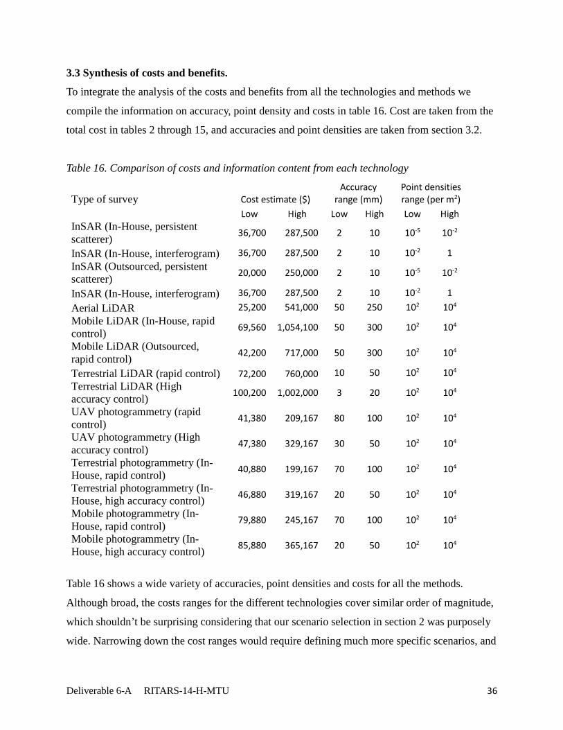
3.3 Synthesis of costs and benefits.

To integrate the analysis of the costs and benefits from all the technologies and methods we

compile the information on accuracy, point density and costs in table 16. Cost are taken from the

total cost in tables 2 through 15, and accuracies and point densities are taken from section 3.2.

Table 16. Comparison of costs and information content from each technology

Type of survey Cost estimate ($) Accuracy

range (mm) Point densities range (per m2)

Low High Low High Low High

InSAR (In-House, persistent scatterer) 36,700 287,500 2 10 10-5 10-2

InSAR (In-House, interferogram) 36,700 287,500 2 10 10-2 1 InSAR (Outsourced, persistent scatterer) 20,000 250,000 2 10 10-5 10-2

InSAR (In-House, interferogram) 36,700 287,500 2 10 10-2 1 Aerial LiDAR 25,200 541,000 50 250 102 104 Mobile LiDAR (In-House, rapid control) 69,560 1,054,100 50 300 102 104

Mobile LiDAR (Outsourced, rapid control) 42,200 717,000 50 300 102 104

Terrestrial LiDAR (rapid control) 72,200 760,000 10 50 102 104 Terrestrial LiDAR (High accuracy control) 100,200 1,002,000 3 20 102 104

UAV photogrammetry (rapid control) 41,380 209,167 80 100 102 104

UAV photogrammetry (High accuracy control) 47,380 329,167 30 50 102 104

Terrestrial photogrammetry (In-House, rapid control) 40,880 199,167 70 100 102 104

Terrestrial photogrammetry (In-House, high accuracy control) 46,880 319,167 20 50 102 104

Mobile photogrammetry (In-House, rapid control) 79,880 245,167 70 100 102 104

Mobile photogrammetry (In-House, high accuracy control) 85,880 365,167 20 50 102 104

Table 16 shows a wide variety of accuracies, point densities and costs for all the methods.

Although broad, the costs ranges for the different technologies cover similar order of magnitude,

which shouldn’t be surprising considering that our scenario selection in section 2 was purposely

wide. Narrowing down the cost ranges would require defining much more specific scenarios, and


that can only be done by defining factors like the geographic, the type of assets being consider,

etc. This is something an agency could more easily do for their area of operation, using the unit

costs discussed in section 2. In-house versus outsourced costs also have similar cost ranges, and

in some cases this was an explicit assumption used in section 2.

The higher costs for in-house scenarios in many cases reflect the fact that initial investment costs

(e. g. buying hardware and software for data collection and analysis) are implicitly spread over

the one year basis assumed for all the calculations, which in a very short time period for the

return on investment in most cases. Spreading the cost related to initial costs for the in-house

scenarios over a period of 3 or 6 years may be a more realistic approach; however, changing the

cost calculations for such cases will not significantly affect the cost ranges shown in table 16, as

most of the costs for those cases comes from the long term components (e. g. data collection and

analysis labor) rather than the initial investment. In summary, as it would be expected, the costs

of developing in-house capacities for data collection and analysis will only be justified if the

work load is large, and over a long enough period of time to recover that investment. For smaller

operations which make less use of the technologies it will could be more economically efficient

to outsource such services.

There is also a clear difference in costs depending on what methods is used to establish control

points for the survey. As it would be expected, the more precise surveying will be more

expensive, especially for large areas. The type of survey used for the control points will also

have an impact on the accuracy, resulting in a tradeoff between cost and accuracy. To achieve

very high accuracies will increase the cost of the survey, but higher accuracies may be needed to

detect very subtle movements or changes in the geotechnical asset surface. Defining the required

level of precision will depend on the asset type and its possible degradation or failure

mechanisms.

The accuracy information given on table 16 also covers overlapping ranges, from a few

millimeters in the case of InSAR, to a few centimeters in the case of LiDAR and SFM

photogrammetry. As discussed in section 3.2.1, there is a noticeable difference between the high

accuracy control and thee rapid control methods, and this is reflected in table 16, by adding 5 to


10 cm of error to the rapid control cases. As discussed previously, there is a tradeoff between the

accuracy of the survey and its cost, and the difference in costs can be substantial; evaluating if

such a cost is justified will depend on how important it is to get very high accuracy data, e. g. in

the case where small deformations could have large consequences.

Point density data in table 16 show a very wide range, from the relatively low point densities of

InSAR data, to the very high point densities of LiDAR and SFM photogrammetry. Applications

over large swaths of a transportation corridor aimed to identify potential problematic areas that

are showing displacement, will not require high point densities, but may require high accuracies

to detect small movements. In such cases InSAR may be the best methods of choice.

Applications over smaller areas, where the details of movement over the scale of a few meters

are relevant, could benefit mostly from the high point densities achieved by LiDAR and SFM

photogrammetry.

LiDAR and SFM photogrammetry methods provide comparable data in terms of cost, accuracies,

and point densities. The initial high cost of LiDAR equipment makes the SFM photogrammetry

attractive for smaller work volume cases. The versatility given by the UAV platform can be an

important advantage for the SFM photogrammetry in some cases, although this does not become

immediately evident from the data here presented. In general the SFM photogrammetry seems to

present a valuable alternative to the LiDAR technology in some cases, but given the status of

LiDAR as a well-tested and established surveying technology, it will take more development and

testing of the SFM photogrammetry methods for its wider adoption as a comparable surveying

technology.

4. Conclusions

Cost estimates for the application of the different remote sensing techniques discussed in this

report vary over a large range of values, mainly because of the wide choice of scenarios chosen

for the analysis. A narrower range of costs can be estimated by choose more specific application

conditions, something a potential user could do using the unit costs given in section 2 as a guide.

Although the estimated costs cover similar ranges in some cases, important differences arise in


between other cases, due to the choice of in-house or outsourcing of the service, as well as the

required level of accuracy.

The choice on whether it is cost effective to develop in-house capabilities or outsource the

service will depend largely on the amount of surveying done by the user. The tradeoff between

cost and accuracy or point density will depend on the specific application of the survey,

particularly, the type of asset being assessed and the type of deterioration or possible failure

mechanism.

The SFM photogrammetric methods seem to deliver results comparable to LiDAR technology,

and in some cases outperform LiDAR products (e. g. the precession test shown in figure 8) for a

lower cost. The viability of SFM seems promising, but we expect that it will requires further

testing and validation before it can be adopted widely as a surveying technology, at the level of

the well-established LiDAR technology. Further testing and validation throughout this project

aims to contribute to this goal.

5. References

AASHTO (2011). Transportation Asset Management Guide, Volume 2: A Focus on Implementation." American Association of State Highway and Transportation Officials. Prepared under NCHRP Project. 69 pp.

Amekudzi, A., M. Meyer, M. Akofio-Sowah, and R. Boadi (2011). Comprehensive

Transportation Asset Management: Making a Business Case and Prioritizing Assets for Inclusion in Formal Asset Management Programs. Technical Report. Georgia Department of Transportation, Office of Materials & Research. 115 pp.

Boardman, A., D. Greenberg, A. Vining, and D. Weimer. (2006). Cost-Benefit analysis. Concept

and Practice. 3rd Edition. Pearson / Prentice Hall. 560 pp. Brooks, C., C. Roussi, T. Colling, M. Watkins, B. Hart, D. Dean, J. Garbarino, R. Dobson, and B.

White (2013). Deliverable 7-B: Performance Evaluation of Recommended Remote Sensing Systems in Unpaved Road Type Condition Characterization. Michigan Tech Research Institute. 78 pp.


Bürgmann, R., Rosen, P.A., and Fielding, E.J., (2000), Synthetic Aperture Radar Interferometry to Measure Earth’s Surface Topography and its Deformation, Annual Review of Earth and Planetary Sciences, 28, 169-209

Cambridge Systematics. (2002) "Transportation Asset Management Guide, Task I–Synthesis of

Asset Management Practice." J. Chang, D. Findley, C. Cunningham, and M. Tsai (2014) Considerations for Effective Lidar

Deployment by Transportation Agencies. Transportation Research Record: Journal of the Transportation Research Board. 2440, 1-8.

Crosetto, M., Monserrat, O.; Iglesias, R.; Crippa, B. (2010) Persistent scatterer interferometry:

Potential, limits and initial C- and X-band comparison. Photogrammetric Engineering and Remote Sensing. 76(9), 1061-1069.

Cutrona, L.J., 1990, Synthetic aperture radar, in Radar Handbook, second edition, Chapter 21,

ed. M. Skolnik, McGraw-Hill, New York Dewberry, (2012). USGS National Enhanced Elevation Assessment. Final Report. 93 pp. Dye Management Group, Inc (2009). Transportation Asset Management Feasibility Study.

Washington State Department of Transportation. 178 pp. Ferretti, A.; Fumagalli, A.; Novali, F.; Prati, C.; Rocca, F.; Rucci, A. (2011) A New Algorithm for

Processing Interferometric Data-Stacks: SqueeSAR. IEEE Transactions on Geoscience and Remote Sensing. 49(9), 3460-3470.

McDougal, J. (2014). Proposal USGS Broad Agency Announcement for 3D Elevation Program.

Southeastern Wisconsin 2015 Regional Lidar and Elevation Data Project. 10 pp. Olsen, M., G. Roe, C. Glennie, F. Persi, M. Reedy, D. Hurwitz, K. Williams, H. Tuss, A.

Squellati, and M. Knodler. (2013) Guidelines for the use of mobile LIDAR in transportation applications. Transportation Research Board. Vol. 748. 208 pp.

Pavelka, K., and J. Šedina. (2015). Creating of DSM Based on RPAS Measurement and

Accuracy Testing. In Růžičková and Inspektor (Editors) Surface Models for Geoscience. Springer. 316 pp.

Sanford Bernhardt, K.L, Loehr, J.E., and Huaco, D., 2003, Asset Management Framework for

Geotechnical Infrastructure, Journal of Infrastructure Systems, 9, 107-116 Sarmap (2009). Synthetic Aperture Radar and SARscape. SAR-Guidebook. 274 pp.

http://www.sarmap.ch/pdf/SAR-Guidebook.pdf Shan, J. and C. Toth. (2009). Topographic Laser Ranging and Scanning. Principles and

Processing. CRC Press. Taylor and Francis Group. 600 pp.

http://www.sarmap.ch/pdf/SAR-Guidebook.pdf


Stanley, D. A. (2011). Asset management in a world of dirt: Emergence of an underdeveloped sector of transportation asset management. TR News, (277).

Stanley, D., and L. Pierson. "Geotechnical Asset Management of Slopes: Condition Indices and

Performance Measures." Geo-Congress 2013 Stability and Performance of Slopes and Embankments III. ASCE. 1651-1660.

State of Michigan. Center for Shared Solutions. 2013. Lidar Pricings. 1 p.

http://www.michigan.gov/documents/cgi/Lidar_Pricing_SOM_CSS_409728_7.pdf Vermont Center for Geographic Information. 2015. Vermont State LiDAR Plan (10th draft). 11

pp. http://vcgi.vermont.gov/sites/vcgi/files/VT%20State%20LiDAR%20Plan_V10.pdf Vessely, M. (2013) Risk Based Methods for Management of Geotechnical Features in

Transportation Infrastructure. In Geo-Congress. Stability and Performance of Slopes and Embankments III (pp. 1625-1632). ASCE.

Vincent, R., and M. Ecker. (2010). Light detection and ranging (LiDAR) technology

evaluation Missouri Department of Transportation Technical, Research, Development and Technology. Report No. OR11-007. 104 pp.

Williams, K., M. Olsen, G., Roe, and C. Glennie. (2013). Synthesis of transportation applications

of mobile LiDAR. Remote Sensing, 5(9), 4652-4692. Yen, K., B. Ravani, and T. Lasky. (2011). LiDAR for Data efficiency. Washington State

Department of Transportation. Office of Research and Library Services. Report No. WA-RD 778.1. 101 pp.

Yen, K., T. Lasky, and B. Ravani. (2014). Cost-Benefit Analysis of Mobile Terrestrial Laser

Scanning Applications for Highway Infrastructure. Journal of Infrastructure Systems, 20(4), 04014022.

Zebker, H.A., Werner, C.L., Rosen, P.A., and Hensley, S., 1994, Accuracy of Topographic Maps

Derived from ERS-1 Interferometric Radar, IEEE Transactions on Geoscience and Remote Sensing, Vol. 32, No. 4, 823-836.

Zerbe, R., and A. Bellas. (2006). A primer for benefit-cost analysis. Edward Elgar Publishing.

316 pp.

http://www.michigan.gov/documents/cgi/Lidar_Pricing_SOM_CSS_409728_7.pdf

http://vcgi.vermont.gov/sites/vcgi/files/VT%20State%20LiDAR%20Plan_V10.pdf

Michigan Technological University - MTRImtri.org/geoasset/media/doc/deliverable_Deliverable...

Documents

Transcript of Michigan Technological University - MTRImtri.org/geoasset/media/doc/deliverable_Deliverable...