MICHAIL ISAAKIDIS Self-organizing Maps for Digital Pre ...
74
Self-organizing Maps for Digital Pre-distortion MICHAIL ISAAKIDIS MASTER´S THESIS DEPARTMENT OF ELECTRICAL AND INFORMATION TECHNOLOGY FACULTY OF ENGINEERING | LTH | LUND UNIVERSITY
Transcript of MICHAIL ISAAKIDIS Self-organizing Maps for Digital Pre ...

Self-organizing Maps for DigitalPre-distortionMICHAIL ISAAKIDISMASTER´S THESISDEPARTMENT OF ELECTRICAL AND INFORMATION TECHNOLOGYFACULTY OF ENGINEERING | LTH | LUND UNIVERSITY
Printed by Tryckeriet i E-huset, Lund 2020
MIC
HA
IL ISAA
KID
ISSelf-organizing M
aps for Digital Pre-distortion
LUN
D 2020
Series of Master’s thesesDepartment of Electrical and Information Technology
LU/LTH-EIT 2020-789http://www.eit.lth.se

Self-organizing Maps for Digital
Pre-distortion
Michail [email protected]
Department of Electrical and Information TechnologyLund University
Supervisors:Liang Liu (LTH)Ove Edfors (LTH)
Asad Jafri (Ericsson)
Examiner: Erik Larsson
September 20, 2020

© 2020Printed in SwedenTryckeriet i E-huset, Lund
List of Acronyms
3GPP 3rd Generation Partnership Project
ACLR Adjacent Channel Leakage Ratio
AM/AM Amplitude to Amplitude
AM/PM Amplitude to Phase
BMU Best Matching Unit
DLA Direct Learning Architecture
DPD Digital Pre-Distortion
DRC Design Rule Check
DSP Digital Signal Processor
FLOPs FLoating point Operations Per second
ILA Indirect Learning Architecture
IMD Intermodulation Distortion
IP Internet Protocol
LS Least Square
LTE Long-Term Evolution
LUT LookUp Table
ML Machine Learning
PA Power Amplifier
PAPI Performance Application Programming Interface
PCA Principal Component Analysis
SOM Self-Organizing Map
W-CDMA Wideband Code Division Multiple Access
i

ii
Abstract
Power amplifiers are very important components in the area of wireless com-munications. However, they are non-linear devices and they seem to achievehigh efficiency when they are operating in the non-linear regions, at the cost ofbeing more power-consuming. In order to linearize their behavior, designershave been considering many methods. Among those, the digital pre-distortiontends to be the most popular one.
There are different ways of applying the digital pre-distortion. Two of themost common are the pseudo-inverse and gradient descent methods. Boththose two methods require too much power, as a result of the high amountof computation. For this reason, new power-efficient methods are under re-search.
The main focus of this master thesis is to explore the possibility of apply-ing the digital pre-distortion with the use of self-organizing maps, a machinelearning algorithm, to develop a more efficient digital pre-distortion (DPD)unit. The algorithm implementation and the simulations were performed withthe use of MATLAB and the neural network toolbox.
During this research, the performance, the accuracy and the computa-tional complexity of the implemented design were measured before and afterthe fine tuning of some of the system’s parameters. The target is to show ifthe use of this algorithm is an efficient method of implementing digital pre-distortion.
iii

iv
Popular Science Summary
Digital pre-distortion: A new approach
The power amplifier is an electronic device that is used in order to increasethe magnitude of the power of a given input signal. It is used for devices likespeakers, headphones and RF transmitters. It is considered as an essentialelement within the wireless communication area, due to the fact that it isused for the transmission and the broadcasting of the signals to the users. Inaddition to those, with the use of power amplifiers and the increase of thepower levels, higher data transfer rates became available. What basically apower amplifier does, from a computation perspective, is that it receives aninput signal and multiplies it with the desired gain. But that is an ideal modelof a power amplifier. However, the power amplifiers are non-linear sourcesfor a communication system, so the real model differs a lot from the idealone. They tend to be non-linear as their output power increases and reachesclose to its maximum value, which can create an in-band distortion withinthe system. For this reason, the linearization of power amplifiers is a veryimportant topic under research in the digital communications field.
The most common method for linearizing a power amplifier’s behavior isthe digital pre-distortion. This method is very power efficient as well as cost-saving. Ideally, with the pre-distortion, the characteristics of a power ampli-fier are inverted in order to compensate for the non-linearities. The role ofa pre-distorter unit inside a digital communication system is to correct anypossible gain and phase nonlinearities and in combination with the system’samplifier to produce a “clear” out of distortion signal. With the use of thepre-distortion and the gain stability that it can provide in the output of theamplifiers, the construction of bigger, more expensive and less efficient ampli-fiers is no longer necessary. Despite the fact that the pre-distortion is widelyand successfully used, it has been observed that the current ways of apply-ing the pre-distortion are very power-consuming due to their complexity andthe amount of computational power they require in order to perform the pre-distortion. For that reason, new approaches are under the scope.
Nowadays, there is a trend in electronics where many concepts are beingimplemented with the use of machine learning in order to replace the number
v

of computations with simpler logic, such as the classification of the data andthe prediction of the desired values. It is easy to understand, that a highamount of computations inside a system means more power which leads to ahigher operating cost. As a result, a more power-efficient system could leadto a big saving in terms of power and money.
This project evaluates the impact of the self-organizing maps algorithmas an adaptive algorithm for the digital pre-distortion. The main goal is toreduce computations and provide a more power-efficient system. It could be aguideline for future researches with new approaches that might lead to moreenergy-saving results.
vi
Contents
1 Background 11.1 Motivation and challenges . . . . . . . . . . . . . . . . . . . . . . 11.2 Power amplifiers . . . . . . . . . . . . . . . . . . . . . . . . . . . . 1
1.2.1 Basic concept 2
1.2.2 Memory effects 3
1.2.3 Intermodulation 3
1.2.4 AM/AM AM/PM Distortions 4
1.3 Machine learning . . . . . . . . . . . . . . . . . . . . . . . . . . . 61.3.1 Types of learning 6
1.3.2 Artificial neural networks 7
1.3.3 The application of machine learning 9
1.4 Thesis structure . . . . . . . . . . . . . . . . . . . . . . . . . . . . 10
2 Digital pre-distortion 112.1 Digital pre-distortion overview . . . . . . . . . . . . . . . . . . . . 112.2 Modeling the amplifier . . . . . . . . . . . . . . . . . . . . . . . . 12
2.2.1 Volterra series 14
2.2.2 Memory polynomial model 15
2.3 Learning architectures . . . . . . . . . . . . . . . . . . . . . . . . 162.4 The conventional approach . . . . . . . . . . . . . . . . . . . . . . 18
2.4.1 Look-Up Table (LUT) based pre-distortion scheme 18
2.5 Figures of merit . . . . . . . . . . . . . . . . . . . . . . . . . . . . 202.5.1 Adjacent-Channel-Power Ratio (ACPR) 20
2.5.2 Error-Vector Magnitude (EVM) 21
2.6 Previous work on digital pre-distortion with machine learning . . 22
3 Self-organizing maps 253.1 Introduction . . . . . . . . . . . . . . . . . . . . . . . . . . . . . . 253.2 Structure . . . . . . . . . . . . . . . . . . . . . . . . . . . . . . . . 263.3 Training a self-organizing map . . . . . . . . . . . . . . . . . . . . 263.4 K-nearest neighbors . . . . . . . . . . . . . . . . . . . . . . . . . . 30
vii
3.5 Applications . . . . . . . . . . . . . . . . . . . . . . . . . . . . . . 31
4 Implementation and results 354.1 Specifications . . . . . . . . . . . . . . . . . . . . . . . . . . . . . 354.2 The concept . . . . . . . . . . . . . . . . . . . . . . . . . . . . . . 354.3 Implementation . . . . . . . . . . . . . . . . . . . . . . . . . . . . 36
4.3.1 Training stage 37
4.3.2 Processing stage 37
4.3.3 Results 39
4.3.4 Optimization loop 42
4.3.5 Results 43
4.4 Architecture . . . . . . . . . . . . . . . . . . . . . . . . . . . . . . 444.5 Computational complexity . . . . . . . . . . . . . . . . . . . . . . 474.6 Comparison to the Look-Up Table (LUT) pre-distorter . . . . . . . 49
5 Conclusions and future work 515.1 Conclusions . . . . . . . . . . . . . . . . . . . . . . . . . . . . . . 515.2 Future work . . . . . . . . . . . . . . . . . . . . . . . . . . . . . . 52
References 53
References 54
viii
List of Figures
1.1 PA behavior. . . . . . . . . . . . . . . . . . . . . . . . . . . . . . . 21.2 Input versus output power for a typical PA. . . . . . . . . . . . . . 21.3 Intermodulation distortion graphical representation. . . . . . . . 41.4 AM/AM and AM/PM plots. . . . . . . . . . . . . . . . . . . . . . . . 51.5 A biological and an artificial neuron [10]. . . . . . . . . . . . . . . 81.6 Artificial neural network architecture, with three input nodes, one
hidden layer, and two output nodes. . . . . . . . . . . . . . . . . 9
2.1 pre-distortion process. . . . . . . . . . . . . . . . . . . . . . . . . 122.2 Digital pre-distortion system block diagram. . . . . . . . . . . . . 122.3 Volterra series structure. . . . . . . . . . . . . . . . . . . . . . . . 162.4 Direct Learning Architecture. . . . . . . . . . . . . . . . . . . . . . 172.5 Indirect Learning Architecture. . . . . . . . . . . . . . . . . . . . . 182.6 DPD with LUT Structure. . . . . . . . . . . . . . . . . . . . . . . . 192.7 Graphical definition of ACPR [3]. . . . . . . . . . . . . . . . . . . . 212.8 EVM measurement. . . . . . . . . . . . . . . . . . . . . . . . . . . 21
3.1 Structure of a SOM network. . . . . . . . . . . . . . . . . . . . . . 263.2 Rectangular topology . . . . . . . . . . . . . . . . . . . . . . . . . 273.3 Hexagonal topology. . . . . . . . . . . . . . . . . . . . . . . . . . . 273.4 Best matching unit. . . . . . . . . . . . . . . . . . . . . . . . . . . 283.5 KNN classification map for Iris flower dataset [44]. . . . . . . . . . 313.6 SOMs-KNN combination. . . . . . . . . . . . . . . . . . . . . . . . 34
4.1 LUT model based on prediction. . . . . . . . . . . . . . . . . . . . 364.2 Training stage, classification of the input values. . . . . . . . . . . 384.3 Processing stage, prediction of the output. . . . . . . . . . . . . . 384.4 Processing stage, prediction of the output. . . . . . . . . . . . . . 394.5 EVM-Classes plot . . . . . . . . . . . . . . . . . . . . . . . . . . . 404.6 ACPR-Classes plot . . . . . . . . . . . . . . . . . . . . . . . . . . . 414.7 EVM-Training size plot . . . . . . . . . . . . . . . . . . . . . . . . . 414.8 ACPR-Training size plot . . . . . . . . . . . . . . . . . . . . . . . . 42
ix
4.9 Training stage with optimization loop. . . . . . . . . . . . . . . . . 424.10 EVM-Number of loops plot . . . . . . . . . . . . . . . . . . . . . . 434.11 ACPR-Number of loops plot . . . . . . . . . . . . . . . . . . . . . . 444.12 Overall system architecture . . . . . . . . . . . . . . . . . . . . . 454.13 Flowchart of the overall process . . . . . . . . . . . . . . . . . . . 464.14 Proposed pre-distorter with SOMs and KNN . . . . . . . . . . . . . 474.15 Pie chart for SOMs complexity . . . . . . . . . . . . . . . . . . . . 48
x

List of Tables
3.1 Iris flower dataset . . . . . . . . . . . . . . . . . . . . . . . . . . . 27
4.1 Performance . . . . . . . . . . . . . . . . . . . . . . . . . . . . . . 394.2 SOMs computational complexity . . . . . . . . . . . . . . . . . . . 484.3 KNN computational complexity . . . . . . . . . . . . . . . . . . . 494.4 Summary of KNN and LUT pre-distorter . . . . . . . . . . . . . . . 49
xi

xii

Chapter1Background
This introductory chapter explores the basic concepts of power amplifiers andmachine learning, that were investigated during this thesis work. By the endof the chapter, the reader will be familiar with all the necessary basic termsand their integration to this project. In addition to that, there will be a discus-sion about the main motivations and the challenges that lead to the choice ofthis topic as a thesis.
1.1 Motivation and challenges
The motivation and the main challenge behind this thesis is to combine twodifferent areas of technology, machine learning, and digital signal processingto provide a more efficient solution for the digital pre-distortion.
The goal is to replace the conventional approaches of digital pre-distortionwith a new one, using the self-organizing maps to reduce the required process-ing power by reducing the number of computations on the forward path of thedigital pre-distortion scheme. Self-organizing maps can identify a correlationbetween the data that can be used in a combination with another algorithm,to form a power-efficient system.
The integration of machine learning into that task is a great challengesince it will introduce a new approach for digital pre-distortion, not based onPA modelling but on patterns. With the self-organizing maps, where the inputsignals are being evaluated and clustered according to their similar features,the pre-distorted signal will be produced based on the formed patterns andpredictions.
1.2 Power amplifiers
This section is an introduction to power amplifiers. The main operation, themost important terms and the basic characteristics of a power amplifier willbe discussed.
1
2 Background
1.2.1 Basic concept
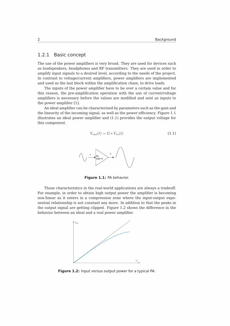
The use of the power amplifiers is very broad. They are used for devices suchas loudspeakers, headphones and RF transmitters. They are used in order toamplify input signals to a desired level, according to the needs of the project.In contrast to voltage/current amplifiers, power amplifiers are implementedand used as the last block within the amplification chain, to drive loads.
The inputs of the power amplifier have to be over a certain value and forthis reason, the pre-amplification operation with the use of current/voltageamplifiers is necessary before the values are modified and sent as inputs tothe power amplifier [1].
An ideal amplifier can be characterized by parameters such as the gain andthe linearity of the incoming signal, as well as the power efficiency. Figure 1.1illustrates an ideal power amplifier and (1.1) provides the output voltage forthis component.
Vout(t) = G ∗ Vin(t) (1.1)
Figure 1.1: PA behavior.
Those characteristics in the real-world applications are always a tradeoff.For example, in order to obtain high output power the amplifier is becomingnon-linear as it enters in a compression zone where the input-output expo-nential relationship is not constant any more. In addition to that the peaks inthe output signal are getting clipped. Figure 1.2 shows the difference in thebehavior between an ideal and a real power amplifier.
Figure 1.2: Input versus output power for a typical PA.
Background 3
According to [2] the non-linearity of a power amplifier can cause the pres-ence of intermodulation products, a topic that will be further discussed in thenext section. This intermodulation could create a leakage into the adjacentchannel of the system and as a result, interference might occur in a differentchannel. The ratio of the average power between the main channel and anadjacent channel is called Adjacent Channel Power Ratio or ACPR. It is alsoknown as Adjacent Channel Leakage Ratio or ACLR [3].
1.2.2 Memory effects
Apart from the amplitude distortions there are also phase distortions that oc-cur in power amplifiers. Those distortions are indicating the presence of mem-ory effects in the amplifier, which means that the output of the PA does notdepend only on the current input but on the previous ones as well [4].
The memory effects can be categorized into two basic types. Electricalmemory effects and electrothermal memory effects. For the first group, theorigin is from the variable impedances at the DC, fundamental and harmonicband. The impedance can be affected by the transistors in the bias network,that they are creating undesired signals into frequencies that the intermodu-lation distortion also occurs (the concept of intermodulation distortion will befurther analyzed in the next section). This source of memory effects is con-sidered as the most important one, due to the fact that it can force many re-strictions on the operation of the system. The second category, electrothermalmemory effects, are occurring due to the difference in transistors propertiesat different temperatures. This effect might create intermodulation distortionas well, however it is not a big issue for low frequencies [5].
1.2.3 Intermodulation
Intermodulation distortion (IMD) could be described as the interaction be-tween two frequencies that are occurring simultaneously in a non-linear de-vice. This interaction will generate unwanted frequencies in the power spec-trum. Real life examples of devices where intermodulation of frequenciescould be observed are the amplifiers and the mixers.
The mixed frequencies will generate intermodulation effects at the pointsof the sum and/or the difference of the integer multiples of the original fre-quencies. Assuming m and n as integers, the output frequency for the mixedinput signals can be expressed from equation (1.2).
mf1 ± nf2 (1.2)
In most cases the IMD is being filtered out, however there are cases wherethe third order IMD is very close to the frequency of the original signal andtherefore it is difficult to filter it. A subset of the third order indermodulationcan be represented by equations (1.3) and (1.4).
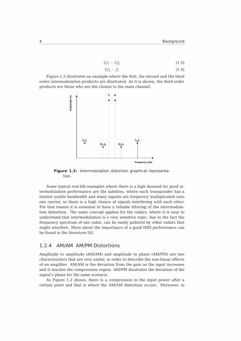
4 Background
2f1 − 2f2 (1.3)
2f2 − f1 (1.4)
Figure 1.3 illustrates an example where the first, the second and the thirdorder intermodulation products are illustrated. As it is shown, the third orderproducts are those who are the closest to the main channel.
Figure 1.3: Intermodulation distortion graphical representa-tion.
Some typical real-life examples where there is a high demand for good in-termodulation performance are the satelites, where each transponder has alimited usable bandwidth and many signals are frequency multiplicated ontoone carrier, so there is a high chance of signals interfering with each other.For that reason it is essential to have a reliable filtering of the intermodula-tion distortion. The same concept applies for the radars, where it is easy tounderstand that intermodulation is a very sensitive topic, due to the fact thefrequency spectrum of one radar, can be easily polluted by other radars thatmight interfere. More about the importance of a good IMD performance canbe found in the literature [6].
1.2.4 AM/AM AM/PM Distortions
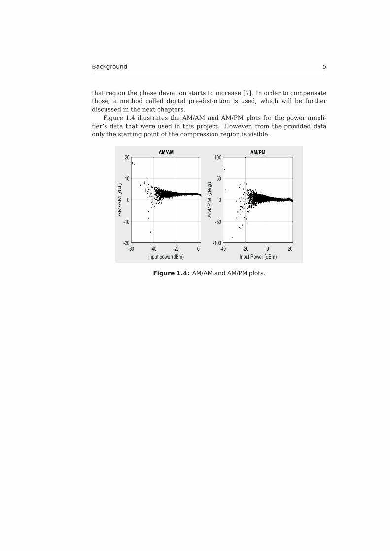
Amplitude to amplitude (AM/AM) and amplitude to phase (AM/PM) are twocharacteristics that are very useful, in order to describe the non-linear effectsof an amplifier. AM/AM is the deviation from the gain as the input increasesand it reaches the compression region. AM/PM illustrates the deviation of thesignal’s phase for the same scenario.
As Figure 1.2 shows, there is a compression in the input power after acertain point and that is where the AM/AM distortion occurs. Moreover, in
Background 5
that region the phase deviation starts to increase [7]. In order to compensatethose, a method called digital pre-distortion is used, which will be furtherdiscussed in the next chapters.
Figure 1.4 illustrates the AM/AM and AM/PM plots for the power ampli-fier’s data that were used in this project. However, from the provided dataonly the starting point of the compression region is visible.
Figure 1.4: AM/AM and AM/PM plots.
6 Background
1.3 Machine learning
Machine learning as a term refers to the computer’s, or machine’s, ability toact without having been explicitly programmed for that. It is considered asa very broad area in our days and it is used in many daily life applicationssuch as speech recognition, movies and music recommendation, auto fillingsentences for email writing and web search. The digital world is so influencedby machine learning, that users are taking advantage of it in many of theirdaily tasks without even knowing about it. The main task of a machine learn-ing algorithm, is to solve very specific problems. However, each algorithm isdifferent depending to the problem that has to be solved.
There are three main categories that the algorithms can be classified asaccording to their ability to learn from patterns:
• Supervised learning, which includes regression and classification.
• Unsupervised learning, which includes clustering and dimensionality re-duction.
• Reinforcement learning, which includes rewards and recommendations.
Each method has its own trade-off and according to the design needs, thedeveloper has to select the most appropriate one.
Reinforcement learning is very popular for artificial intelligence in thevideo gaming industry, as well as for the navigation of robots. Supervisedlearning is used more for predictions. For example weather forecasting orprediction and analysis of stock market, as well as data classification, whichis a strong tool in image processing. Unsupervised learning is a very effectiveapproach for feature extraction, visualization of big data sets and effectiveclustering of data.
In this project a combination of unsupervised and supervised learning isused, so those two concepts will be further explained in this section.
1.3.1 Types of learning
Supervised learning
Talking about supervised learning the most important characteristic that candefine this type of learning is the presence of annotated training data, alsoknown as labels. Supervised algorithms are using known datasets with knownlabels and they perform predictions on new datasets with undefined labels. Inother words, it is the process of teaching a model by providing a combinationof input and output data.
There are two categories of supervised learning algorithms:
• Classification, where the labels are classes, so the system is trainedto provide specific classes to a new dataset. A typical example of aclassifier is an algorithm that determinates if an email is spam or not.
Background 7
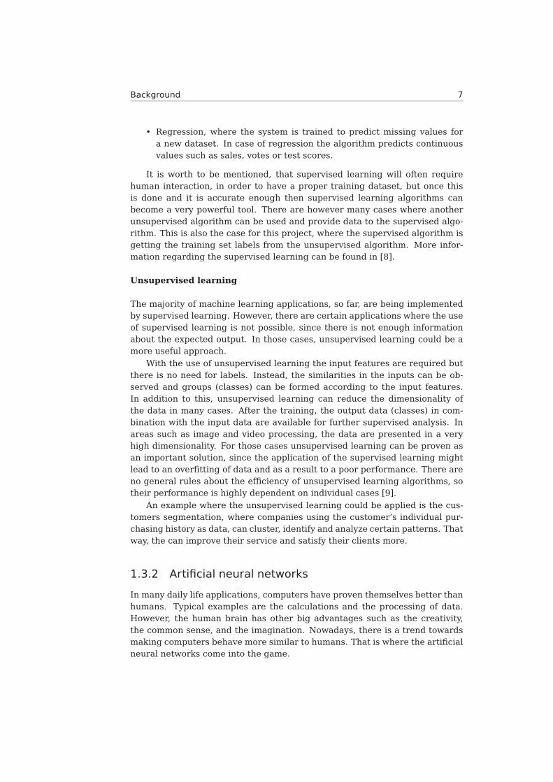
• Regression, where the system is trained to predict missing values fora new dataset. In case of regression the algorithm predicts continuousvalues such as sales, votes or test scores.
It is worth to be mentioned, that supervised learning will often requirehuman interaction, in order to have a proper training dataset, but once thisis done and it is accurate enough then supervised learning algorithms canbecome a very powerful tool. There are however many cases where anotherunsupervised algorithm can be used and provide data to the supervised algo-rithm. This is also the case for this project, where the supervised algorithm isgetting the training set labels from the unsupervised algorithm. More infor-mation regarding the supervised learning can be found in [8].
Unsupervised learning
The majority of machine learning applications, so far, are being implementedby supervised learning. However, there are certain applications where the useof supervised learning is not possible, since there is not enough informationabout the expected output. In those cases, unsupervised learning could be amore useful approach.
With the use of unsupervised learning the input features are required butthere is no need for labels. Instead, the similarities in the inputs can be ob-served and groups (classes) can be formed according to the input features.In addition to this, unsupervised learning can reduce the dimensionality ofthe data in many cases. After the training, the output data (classes) in com-bination with the input data are available for further supervised analysis. Inareas such as image and video processing, the data are presented in a veryhigh dimensionality. For those cases unsupervised learning can be proven asan important solution, since the application of the supervised learning mightlead to an overfitting of data and as a result to a poor performance. There areno general rules about the efficiency of unsupervised learning algorithms, sotheir performance is highly dependent on individual cases [9].
An example where the unsupervised learning could be applied is the cus-tomers segmentation, where companies using the customer’s individual pur-chasing history as data, can cluster, identify and analyze certain patterns. Thatway, the can improve their service and satisfy their clients more.
1.3.2 Artificial neural networks
In many daily life applications, computers have proven themselves better thanhumans. Typical examples are the calculations and the processing of data.However, the human brain has other big advantages such as the creativity,the common sense, and the imagination. Nowadays, there is a trend towardsmaking computers behave more similar to humans. That is where the artificialneural networks come into the game.
8 Background
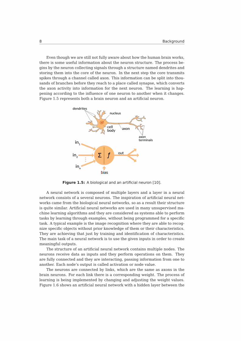
Even though we are still not fully aware about how the human brain works,there is some useful information about the neuron structure. The process be-gins by the neuron collecting signals through a structure named dendrites andstoring them into the core of the neuron. In the next step the core transmitsspikes through a channel called axon. This information can be split into thou-sands of branches before they reach to a place called synapse, which convertsthe axon activity into information for the next neuron. The learning is hap-pening according to the influence of one neuron to another when it changes.Figure 1.5 represents both a brain neuron and an artificial neuron.
Figure 1.5: A biological and an artificial neuron [10].
A neural network is composed of multiple layers and a layer in a neuralnetwork consists of a several neurons. The inspiration of artificial neural net-works came from the biological neural networks, so as a result their structureis quite similar. Artificial neural networks are used in many unsupervised ma-chine learning algorithms and they are considered as systems able to performtasks by learning through examples, without being programmed for a specifictask. A typical example is the image recognition where they are able to recog-nize specific objects without prior knowledge of them or their characteristics.They are achieving that just by training and identification of characteristics.The main task of a neural network is to use the given inputs in order to createmeaningful outputs.
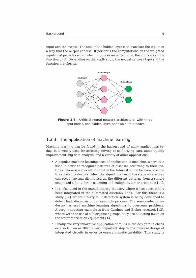
The structure of an artificial neural network contains multiple nodes. Theneurons receive data as inputs and they perform operations on them. Theyare fully connected and they are interacting, passing information from one toanother. Each node’s output is called activation or node value.
The neurons are connected by links, which are the same as axons in thebrain neurons. For each link there is a corresponding weight. The process oflearning is being implemented by changing and adjusting the weight values.Figure 1.6 shows an artificial neural network with a hidden layer between the
Background 9
input and the output. The task of the hidden layer is to translate the inputs ina way that the output can use. It performs the computations on the weightedinputs and provides a net, which produces an output after the application of afunction on it. Depending on the application, the neural network type and thefunction are chosen.
Figure 1.6: Artificial neural network architecture, with threeinput nodes, one hidden layer, and two output nodes.
1.3.3 The application of machine learning
Machine learning can be found in the background of many applications to-day. It is widely used for assisting driving or self-driving cars, audio qualityimprovement, big data analysis, and a variety of other applications.
• A popular machine learning area of application is medicine, where it isused in order to recognize patterns of diseases according to their fea-tures. There is a speculation that in the future it would be even possibleto replace the doctors, when the algorithms reach the stage where theycan recognize and distinguish all the different patterns from a simplecough and a flu, to brain scanning and malignant tumor prediction [11].
• It is also used in the manufacturing industry where it has successfullybeen integrated in the automated assembly lines. For this there is astudy [12], where a fuzzy fault detection system is being developed todetect fault diagnosis of car assembly process. The semiconductor in-dustry has used machine learning algorithms to overcome problems.A very interesting example is from Gardner and Bieker research [13],where with the use of self-organizing maps, they are detecting faults onthe wafer fabrication equipment [14].
• Finally one very innovative application of ML is in the design rule checkor also known as DRC, a very important step in the physical design ofintegrated circuits in order to ensure manufacturability. This study is
10 Background
based on the following papers [15], [16] and [17], where a variety of fea-tures that can lead to DRC violations are identified. During the place-ment and the global routing those features are extracted and feed tothe neural network as training inputs, in combination with the actualDRC result. After some certain number of training and evaluation stepsthe model is ready to be used and predict design rule violation hotspots[18].
Nowadays, machine learning is getting more popular since the availablehardware resources, that are needed for training machine learning models,are more powerful. In addition to that new and more efficient machine learn-ing algorithms are introduced continuously. This is only the start towards anew generation where the use of machine learning will offer efficient and lowpower consuming electronic devices.
1.4 Thesis structure
The thesis is organized into the following chapters:
· Chapter 1: The background and the basic concepts and terminology ofthe thesis.
· Chapter 2: A theoretical analysis of digital pre-distortion and all therelated concepts, with an introduction to the conventional digital pre-distortion approaches.
· Chapter 3: The self-organizing maps are presented along with usefulinformation that will help the reader to understand their main function-alities.
· Chapter 4: The implementation steps and the recorded results for thisproject are presented.
· Chapter 5: The main conclusion points of the project in along with sug-gestions about future work.
Chapter2Digital pre-distortion
As mentioned in the previous chapter, power amplifiers are more efficient interms of performance, when they are operating in their compression (non-linear) region. However, in that region the peaks are getting clipped and asa result the output frequency spectrum is ruined. To avoid this, the clippingcould be estimated from before, in order to form the inverse model and com-pensate the amplifier’s loss, in terms of gain. When this concept is appliedto systems with high bandwidths, the memory effects must be considered,otherwise the performance could be affected due to the fact that when thebandwidth increases the memory depth of the power amplifier also increases[19].
Digital pre-distortion is considered as the most efficient technique of lin-earization for power amplifiers, in terms of good linearization performanceand low implementation complexity. In the following sections of this chapter,the concepts and the terminology of the digital pre-distortion will be furtherdiscussed.
2.1 Digital pre-distortion overview
In order to apply digital pre-distortion to a power amplifier, a good first stepwould be to extract its behaviour. This can be achieved by observing the inputand the output data of the PA. The next step is the observation and the esti-mation of the memory effects through the amplitude-to-amplitude modulation(AM/AM) and the amplitude-to-phase modulation (AM/PM) plots. When theeffects are estimated then the inverse equivalent for the input signal shouldbe constructed in order to remove the estimated distortions.
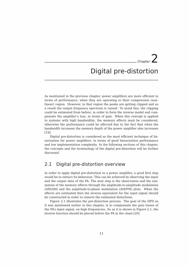
Figure 2.1 illustrates the pre-distortion process. The goal of the DPD asit was mentioned earlier in this chapter, is to compensate the gain losses ofthe PA’s input signal, on high frequencies. So as it is shown in Figure 2.1, theinverse function should be placed before the PA in the chain [20].
11
12 Digital pre-distortion
Figure 2.1: pre-distortion process.
The results of the DPD can be evaluated through the ACPR, EVM and someother parameters that will be further explained in section 2.2.1.
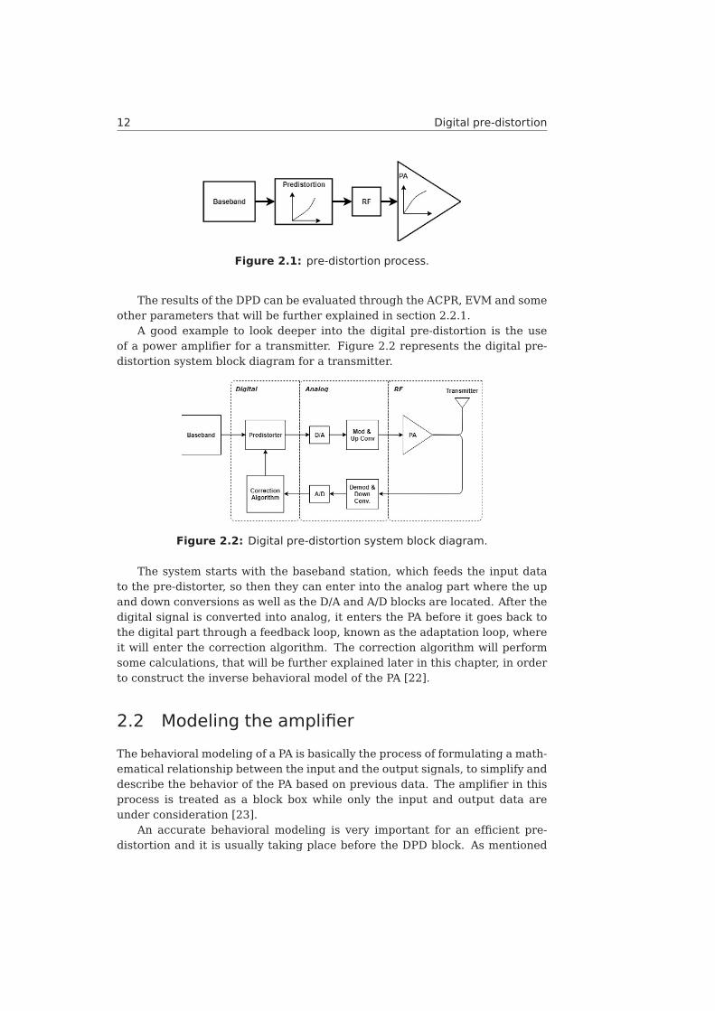
A good example to look deeper into the digital pre-distortion is the useof a power amplifier for a transmitter. Figure 2.2 represents the digital pre-distortion system block diagram for a transmitter.
Figure 2.2: Digital pre-distortion system block diagram.
The system starts with the baseband station, which feeds the input datato the pre-distorter, so then they can enter into the analog part where the upand down conversions as well as the D/A and A/D blocks are located. After thedigital signal is converted into analog, it enters the PA before it goes back tothe digital part through a feedback loop, known as the adaptation loop, whereit will enter the correction algorithm. The correction algorithm will performsome calculations, that will be further explained later in this chapter, in orderto construct the inverse behavioral model of the PA [22].
2.2 Modeling the amplifier
The behavioral modeling of a PA is basically the process of formulating a math-ematical relationship between the input and the output signals, to simplify anddescribe the behavior of the PA based on previous data. The amplifier in thisprocess is treated as a block box while only the input and output data areunder consideration [23].
An accurate behavioral modeling is very important for an efficient pre-distortion and it is usually taking place before the DPD block. As mentioned
Digital pre-distortion 13
earlier, the concept of the digital pre-distortion is to construct an inverse be-havioral model of the PA and for that reason, there is a need for a good andsimple behavioral model of the PA.
The behavioural models for power amplifiers are divided into the two fol-lowing categories.
Memoryless models
This model considers only the current input data and ignores any past ones,so the output depends only on the current input. The distortion is usually sep-arated into two different distortions, the AM/AM and the AM/PM distortions.The AM/AM is modelling the PAs saturated output signal and the AM/PM thephase shift of the signal.
The relationship between the input and the output can be expressed as
zbp(n) = F ∗ xbp(n) (2.1)
where xbp corresponds to the bandpass input, zbp to the bandpass output, Fto the function of nonlinearity and n to time-domain sampling index.
Some popular memoryless models are:
• The Saleh model
• The Ghorbani model
• The Rapp model
• Bessel-Fourier
Those four memoryless models are providing different accuracy for a be-havioural model, depending on the PAs operating region. More informationabout them can be found in the literature [24].
Memory-based models
In contrast with memoryless models, models with memory are considering notonly the current input data but also the previous ones, for a specific range.This means that the current and the past inputs will effect the output andby this condition the system will automatically be converted into a dynamicsystem.
The memory models are commonly used for systems with wide signalbandwidths, up to 100MHz, without introducing memory effects. However,high-power amplifiers in wireless base stations use wider bandwidths. Forthose systems memoryless pre-distortion can achieve very limited results oflinearization and for this reason memory-based models are preferable.
The most common algorithms for models with memory are the following :
• Volterra series
14 Digital pre-distortion
• Wiener, Hammerstein and Wiener-Hammerstein
• Memory polynomial
• Generalized memory polynomial
• Neural networks
• LUT pre-distorter
Volterra series, Wiener, Hammerstein and Wiener-Hammerstein are con-sidered as some of the most popular pre-distortion algorithms for models withmemory. However, those methods are introducing a big number of coeffi-cients which could be very complex for practical applications. For this reason,there are other methods, such as the Memory polynomial and the Generalizedmemory polynomial that are based on the Volterra series but are less compli-cated [17]. In addition to those, the LUT pre-distorter according to [25] can beproved as a low cost, efficient, and flexible method for systems with low degreeof non-linearity and memory depth. As those two parameters are increasing,the size of the LUTs will increase as well, which will affect the design’s area.At last, the neural network approach is very different than the others. In sim-ple terms, it can be described as a network that tries to behave as the humanbrain and learn from past knowledge and specific patterns. When it acquiresthe required knowledge it can predict the desired values, in the case of digitalpre-distorition, the pre-distorter’s output values.
In this chapter the main focus will be on the LUT pre-distorter, due tothe fact that the initial measurements and the comparison with the machinelearning approach were made with that one. The suggested implementationtries to integrate the LUT pre-distorter into the neural network approach andwill be explained in Chapter 4. This technique is based on the the memorypolynomial model which will be explained in this section. However, in order tounderstand the memory polynomial model, it is necessary first to understandthe Volterra series, since the memory polynomial is a special and simplifiedcase of Volterra series.
2.2.1 Volterra series
Volterra series is considered as a series of functionals. In other words, aseries of operations which are assigning functions to specific sets. It is away of modeling nonlinear systems with memory, so it is a good tool to modelthe behavior of a power amplifier with memory by describing its input-outputrelationship. However, Volterra series shows a very high complexity in termsof computations and as a result it is considered as an impractical solution forreal applications such as hardware designing. The number of computations forVolterra series is high because of the large number of parameters, a numberthat increases exponentially along with the degree of non-linearity and thedepth of the memory that the system has [21].
Digital pre-distortion 15
Volterra series can be expressed with the following equation for the dis-crete time domain:
y(n) =
P∑p=1
M∑ii=0
...
M∑ip=0
hp(ii, .., ip)
p∏j=1
x(n− ij) (2.2)
where hp is the kernel of Volterra series, x the input of the system and y theoutput. P is degree of nonlinearity and M the memory depth.
Volterra series kernels are the coefficients that are defining the targetmodel. When the coefficients are estimated then the system is ready to bemodeled for any input value.
The coefficients are being estimated with the use of the least square ap-proach and the target is the minimization of the sum squared error betweenthe observed data and the output of the PA model. This process is describedby the following equation:
J(θ) =N−1∑n=0
e2(n) =N−1∑n=0
| y(n)− y′(n) |2 (2.3)
where N is the number of the input samples, y(n) are the samples of the pre-distorter’s observed output data and y′(n) are the PAs output data [26].
Those coefficients can be expressed as:
hp = (XHX)−1XHy = X+y (2.4)
where (.)h denotes the Hermitian transpose and (.)+ the Moore-Penrose pseudo-inverse. X is the Volterra terms of the input signal x, and y is the capturedoutput signal. With the use of this equation and the input, output signals thecoefficient can be estimated and the modeling of the PA can be achieved.
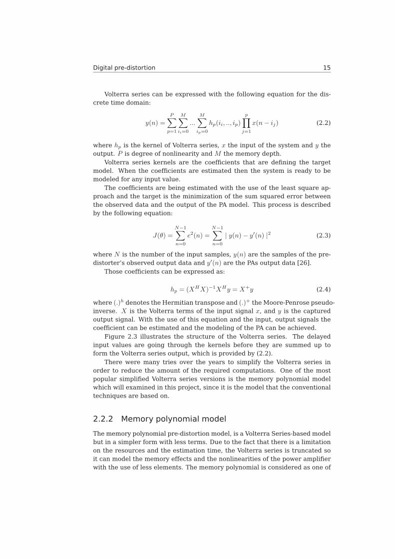
Figure 2.3 illustrates the structure of the Volterra series. The delayedinput values are going through the kernels before they are summed up toform the Volterra series output, which is provided by (2.2).
There were many tries over the years to simplify the Volterra series inorder to reduce the amount of the required computations. One of the mostpopular simplified Volterra series versions is the memory polynomial modelwhich will examined in this project, since it is the model that the conventionaltechniques are based on.
2.2.2 Memory polynomial model
The memory polynomial pre-distortion model, is a Volterra Series-based modelbut in a simpler form with less terms. Due to the fact that there is a limitationon the resources and the estimation time, the Volterra series is truncated soit can model the memory effects and the nonlinearities of the power amplifierwith the use of less elements. The memory polynomial is considered as one of
16 Digital pre-distortion
Figure 2.3: Volterra series structure.
the most effective truncated versions and it is expressed with the use of thefollowing formula:
y(n) =P∑
p=1
M∑m=0
cp,mx(n−m) | x(n−m) |p−1 (2.5)
where x is the input signal, y the output, c the coefficients and P and M thedegree of nonlinearity and the memory depth respectively [27].
2.3 Learning architectures
There are two different architectures that are used for pre-disorters withmemory structures. The first one receives the power amplifier’s output andinverses it directly. This method is called direct learning architecture (DLA).The second one constructs a pre-distorter with the use of a postdistorter andit is called indirect learning architecture (IDLA).
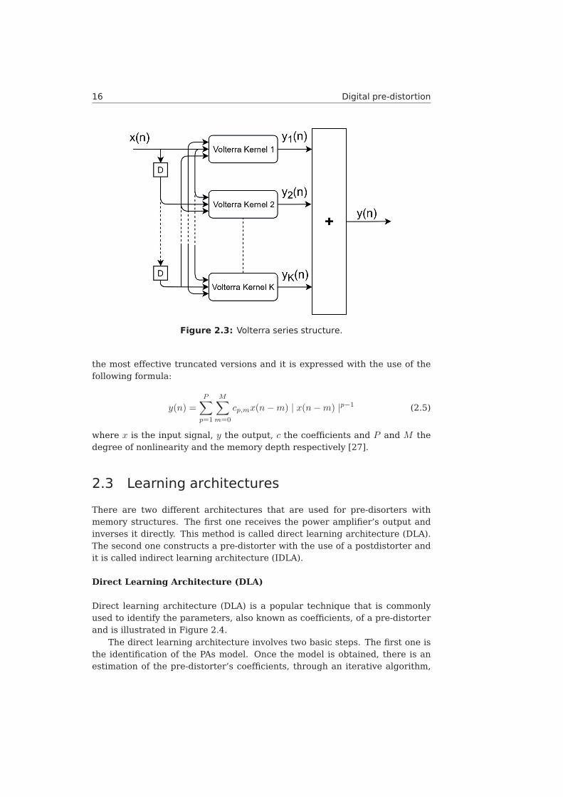
Direct Learning Architecture (DLA)
Direct learning architecture (DLA) is a popular technique that is commonlyused to identify the parameters, also known as coefficients, of a pre-distorterand is illustrated in Figure 2.4.
The direct learning architecture involves two basic steps. The first one isthe identification of the PAs model. Once the model is obtained, there is anestimation of the pre-distorter’s coefficients, through an iterative algorithm,
Digital pre-distortion 17
Figure 2.4: Direct Learning Architecture.
that tries to minimize the error between the desired and the actual output, seeequation (2.6). The goal is to drive the output z(n) as close as possible to x(n).For that reason the learning controller e is used as a mean of measuring theirdifference.
e(n) = x(n)− z(n) (2.6)
After the extraction of the coefficients the next step is to use them in orderto construct a pre-distorted signal that will be applied to the PA. This pro-cess takes place in the pre-distorter block and it is an iterative process thatcontinues until the best possible solution has been identified.
There are different algorithms that can be used for direct learning archi-tecture, however this architecture is not very popular due to its structuralcomplexity and the big amount of computations that requires [25].
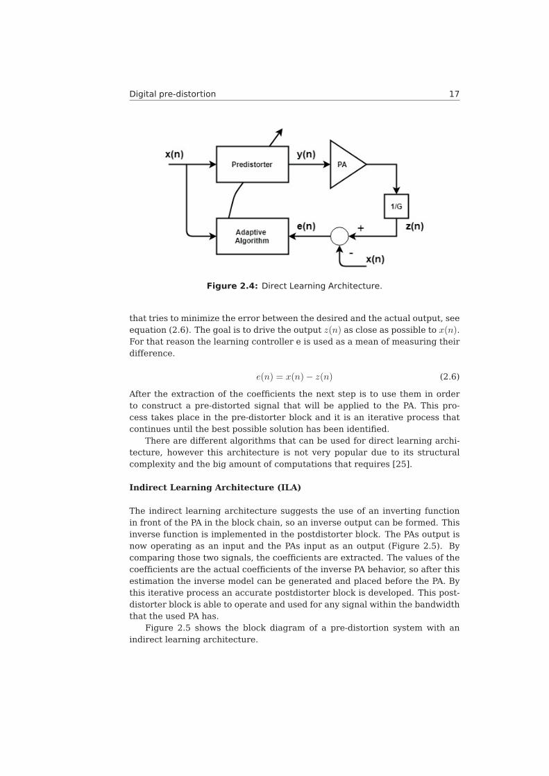
Indirect Learning Architecture (ILA)
The indirect learning architecture suggests the use of an inverting functionin front of the PA in the block chain, so an inverse output can be formed. Thisinverse function is implemented in the postdistorter block. The PAs output isnow operating as an input and the PAs input as an output (Figure 2.5). Bycomparing those two signals, the coefficients are extracted. The values of thecoefficients are the actual coefficients of the inverse PA behavior, so after thisestimation the inverse model can be generated and placed before the PA. Bythis iterative process an accurate postdistorter block is developed. This post-distorter block is able to operate and used for any signal within the bandwidththat the used PA has.
Figure 2.5 shows the block diagram of a pre-distortion system with anindirect learning architecture.
18 Digital pre-distortion
Figure 2.5: Indirect Learning Architecture.
The advantage of this architecture compared to the direct learning, is thatit does not require the modelling assumption and the estimation of the PAscoefficients, since the process occurs after the signal leaves the PA and thePAs output is known [20].
In this thesis the indirect learning architecture is used in both the LUTbased and the SOMs approach. For the first one it will be explained in moredetail in the upcoming sections 2.4.1. For the SOMs approach it will be dis-cussed in Chapter 4 (section 4.4).
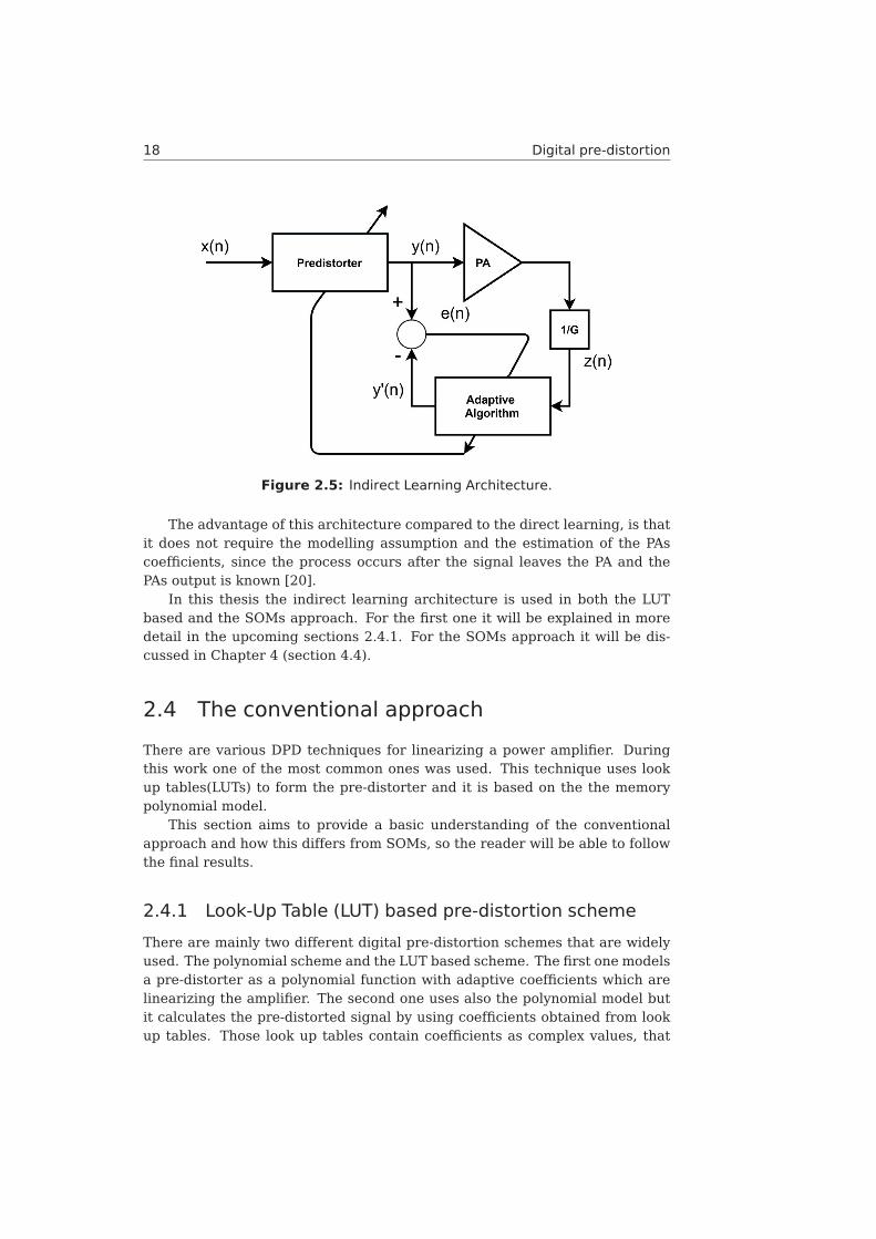
2.4 The conventional approach
There are various DPD techniques for linearizing a power amplifier. Duringthis work one of the most common ones was used. This technique uses lookup tables(LUTs) to form the pre-distorter and it is based on the the memorypolynomial model.
This section aims to provide a basic understanding of the conventionalapproach and how this differs from SOMs, so the reader will be able to followthe final results.
2.4.1 Look-Up Table (LUT) based pre-distortion scheme
There are mainly two different digital pre-distortion schemes that are widelyused. The polynomial scheme and the LUT based scheme. The first one modelsa pre-distorter as a polynomial function with adaptive coefficients which arelinearizing the amplifier. The second one uses also the polynomial model butit calculates the pre-distorted signal by using coefficients obtained from lookup tables. Those look up tables contain coefficients as complex values, that
Digital pre-distortion 19
are multiplied with the input signal, according to the input signal’s amplitude.The look up table scheme is used in this thesis as a conventional approach.
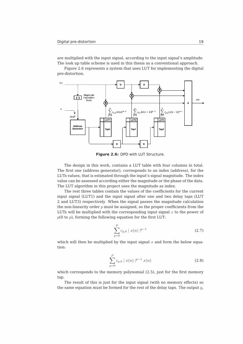
Figure 2.6 represents a system that uses LUT for implementing the digitalpre-distortion.
Figure 2.6: DPD with LUT Structure.
The design in this work, contains a LUT table with four columns in total.The first one (address generator), corresponds to an index (address), for theLUTs values, that is estimated through the input’s signal magnitude. The indexvalue can be assessed according either the magnitude or the phase of the data.The LUT algorithm in this project uses the magnitude as index.
The rest three tables contain the values of the coefficients for the currentinput signal (LUT1) and the input signal after one and two delay taps (LUT2 and LUT3) respectively. When the signal passes the magnitude calculationthe non-linearity order p must be assigned, so the proper coefficients from theLUTs will be multiplied with the corresponding input signal x to the power ofp(0 to p), forming the following equation for the first LUT:
P∑p=0
cp,0 | x(n) |p−1 (2.7)
which will then be multiplied by the input signal x and form the below equa-tion:
P∑p=0
cp,0 | x(n) |p−1 x(n) (2.8)
which corresponds to the memory polynomial (2.5), just for the first memorytap.
The result of this is just for the input signal (with no memory effects) sothe same equation must be formed for the rest of the delay taps. The output y,
20 Digital pre-distortion
which corresponds to the pre-distorter’s output and the PA’s input, will be thesum of those equations for each memory tap. For example if the result of (2.8)is considered as y1(n) and the system has three memory taps in total whichgive y2(n) and y3(n) for x(n− 1) and x(n− 2) respectively, the final y would bethe sum of those :
y(n) = y1(n) + y2(n) + y3(n) (2.9)
The equations (2.9) and (2.10) including M number of memory taps will be-come as follow to provide the final y:
y(n) =P∑
p=0
M∑m=0
cp,m | x(n−m) |p−1 x(n−m) (2.10)
which is the memory polynomial equation explained in the previous section by(2.5). The output y, result of the multiplication, will be converted into RF andfed into the PA.
In the feedback loop, an adaptive process is taking place, where the valuesinside the LUTs are updated constantly, through the Volterra Series and theleast square approach described previously. This update of the values corre-sponds to the changes in the PAs behavior over the time. The changes areusually caused by factors such as ageing and temperature. The update pro-cess considers the output of the PA, the input of the PA and the index value inorder to estimate these changes [28].
2.5 Figures of merit
By definition a figure of merit is the way of characterizing a system’s perfor-mance in terms of quantity and compare it to its alternatives. In this projectthe Adjacent Channel Power Ratio (ACPR) is used as a measure of perfor-mance and the Error-Vector Magnitude (EVM) as a measure of accuracy.
2.5.1 Adjacent-Channel-Power Ratio (ACPR)
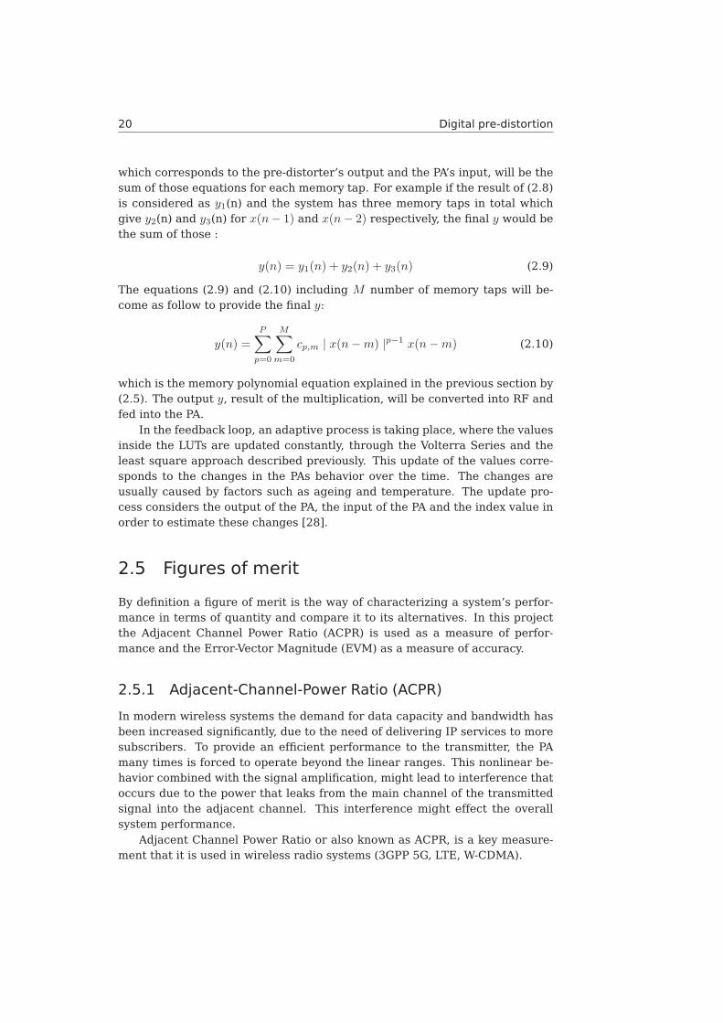
In modern wireless systems the demand for data capacity and bandwidth hasbeen increased significantly, due to the need of delivering IP services to moresubscribers. To provide an efficient performance to the transmitter, the PAmany times is forced to operate beyond the linear ranges. This nonlinear be-havior combined with the signal amplification, might lead to interference thatoccurs due to the power that leaks from the main channel of the transmittedsignal into the adjacent channel. This interference might effect the overallsystem performance.
Adjacent Channel Power Ratio or also known as ACPR, is a key measure-ment that it is used in wireless radio systems (3GPP 5G, LTE, W-CDMA).
Digital pre-distortion 21
As Figure 2.7 illustrates, it is defined as the ratio of the modulated signalpower in the main channel and the power leaked into the adjacent channeland it is measured in decibels relative to the carrier (dBc) [3].
Figure 2.7: Graphical definition of ACPR [3].
2.5.2 Error-Vector Magnitude (EVM)
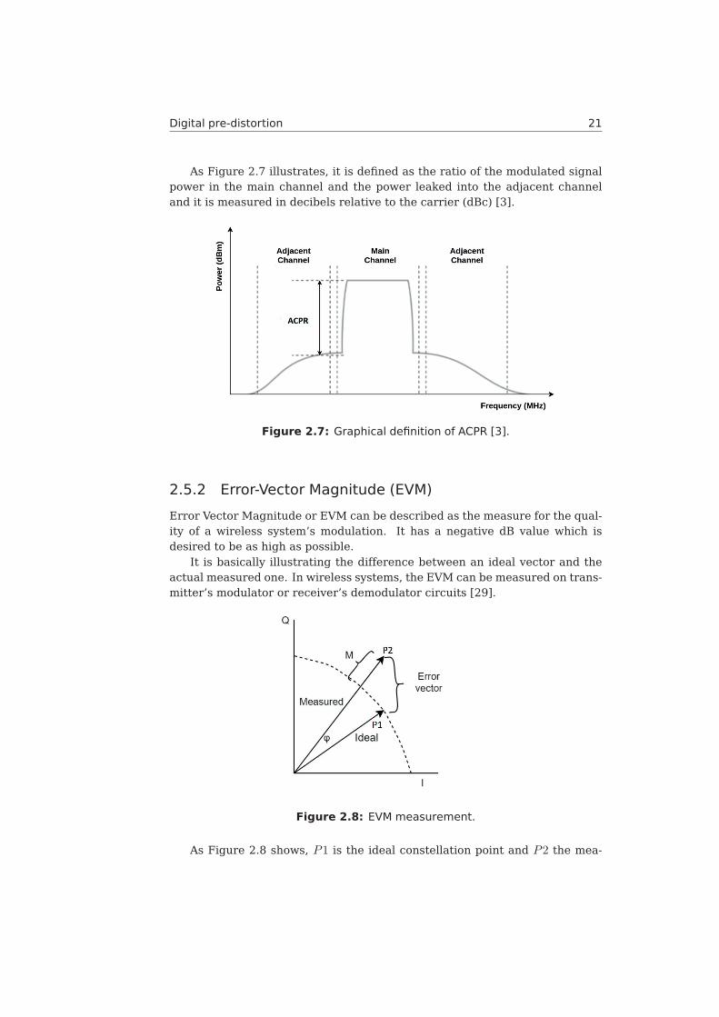
Error Vector Magnitude or EVM can be described as the measure for the qual-ity of a wireless system’s modulation. It has a negative dB value which isdesired to be as high as possible.
It is basically illustrating the difference between an ideal vector and theactual measured one. In wireless systems, the EVM can be measured on trans-mitter’s modulator or receiver’s demodulator circuits [29].
Figure 2.8: EVM measurement.
As Figure 2.8 shows, P1 is the ideal constellation point and P2 the mea-
22 Digital pre-distortion
sured one. The difference among them might be due to many reasons such asIQ mismatch (gain, phase, DC offset), frequency offset, phase noise, AM-AMdistortion, AM-PM distortion etc. The M and φ shows the magnitude and thephase error respectively [30]. The EVM can be expressed by the followingequation:
EVM =
√(I2− I1)2 + (Q2−Q1)2
| P1 | (2.11)
where, P1 = I1+j ∗Q1 is the ideal vector and P2 = I2+j ∗Q2 is the measuredvector.
The EVM is expressed as:
EVMdb = 10 ∗ log10[EVMrms
100] (2.12)
which provides the result in dB.EVM can also be measured as a percentage:
EVMrms = 100 ∗ 10((EVM)dB/20) (2.13)
2.6 Previous work on digital pre-distortion withmachine learning
Digital pre-distortion can be implemented in many different ways and providedifferent results respectively. The use of machine learning algorithms andneural networks has become very popular nowadays, due to their ability ofreducing the complexity and the number of computation within an embeddeddevice. This section will examine some of the existing researches that areclosely related to the work of this thesis, and their results.
An interesting project is from Manish Sonal (2016). This research exploresthe modeling of nonlinear analog devices, such as Power Amplifier (PA), withthe use of machine learning algorithms. Some of the algorithms that wereused and compared in this study are nonlinear regression, smoothing spline,polynomial fit and deep learning with the use of Levenberg–Marquardt algo-rithm. The results are indicating that the deep learning method provides avery good estimation of the data while it was more time consuming and re-quired more CPU memory [31]. This need however, was a result of the bigamount of the neurons and hidden layers, which is not considered as an issuein the use of self-organizing maps, due to their simpler structure.
In contrast with Manish Sonal (2016), Zhenyu Wang et al (2017) proposesa novel method based on deep neural networks, auto-encoder model, for thedigital pre-distortion and the results are indicating two things as advantages.The first one is that the deep neural networks are providing a higher accuracyand can fit nonlinear models with success. The second one is that the processspeed after each iteration will be faster, due to their deep network structure,
Digital pre-distortion 23
than the traditional neural networks, which basically means that they have theability to learn and perform faster on practical applications [32].
One good example of digital pre-distortion with the use of a machine learn-ing algorithm, comes from Jun Peng et al. (2016), where the digital pre-distortion is applied with the use of Spare Bayesian learning. What that al-gorithm does basically is predicting, based on probability, the parameters andthe behavioral model of the power amplifier. The results shown that by ap-plying the Spare Bayesian approach the parameters and the sampling wherereduced significantly, compared to conventional methods, while the modellingaccuracy was very satisfying. This approach is very similar to the SOMs ap-proach but the main difference is that Spare Bayesian is a supervised ap-proach, when self-organizing maps is an unsupervised one [33].
Finally, James Peroulas (2016) research examines the implementation ofthe pre-distortion with the use of five different machine learning algorithmsand how effective they are compared to the memory polynomial approach,which is also used as a conventional algorithm in this thesis work. The five al-gorithms are linear regression, regularization, model selection, principal com-ponent analysis, and gradient descent. Principal component analysis (PCA),which is a method similar to the self-organizing maps, provided the best re-sults by reducing the number of computations significantly and maintainedthe performance at acceptable levels [34].

24 Digital pre-distortion
Chapter3Self-organizing maps
3.1 Introduction
A self-organizing map (SOM), is an artificial neural network (ANN) which ap-plies a competitive learning approach to train samples for data analysis. Themost popular self-organizing maps model is known as the Kohonen networkand it was introduced in 1982 by the Finnish researcher Teuvo Kohonen. Itis considered as a special type of artificial network and it is widely used forclustering and visualizing data [35].
The main principle of self-organizing maps is the transformation of com-plex data with high-dimensionality, into a simpler form with fewer dimensions(usually two). The location (coordinates) of the output nodes is extractedthrough the common characteristics of the input space elements. This aspectmakes this method similar to other popular dimensionality-reduction tech-niques, such as the principal component analysis. However, SOMs are provedto have key features that make them more efficient. For example, their imple-mentation is easier, and they are very effective in solving nonlinear problemswith a high degree of complexity. In addition to this, they perform very wellwith noisy or missing data and big datasets, compare to other techniques.
Self-organizing maps are categorized as an unsupervised learning algo-rithm. As it was mentioned in Chapter 1, unsupervised algorithms do notdepend on predefined outputs during their process. In other words, these al-gorithms learn through observation and draw inferences, rather than depend-ing on input datasets with labels. For self-organizing maps, this happens byapplying competitive learning rules to their output nodes, which are compet-ing with each other. Through the learning process, the information is headingonly to one direction, without using any feedback loop. This makes SOMs afeedforward network. The input and output nodes are connected through links(weights) [36].
25
26 Self-organizing maps
3.2 Structure
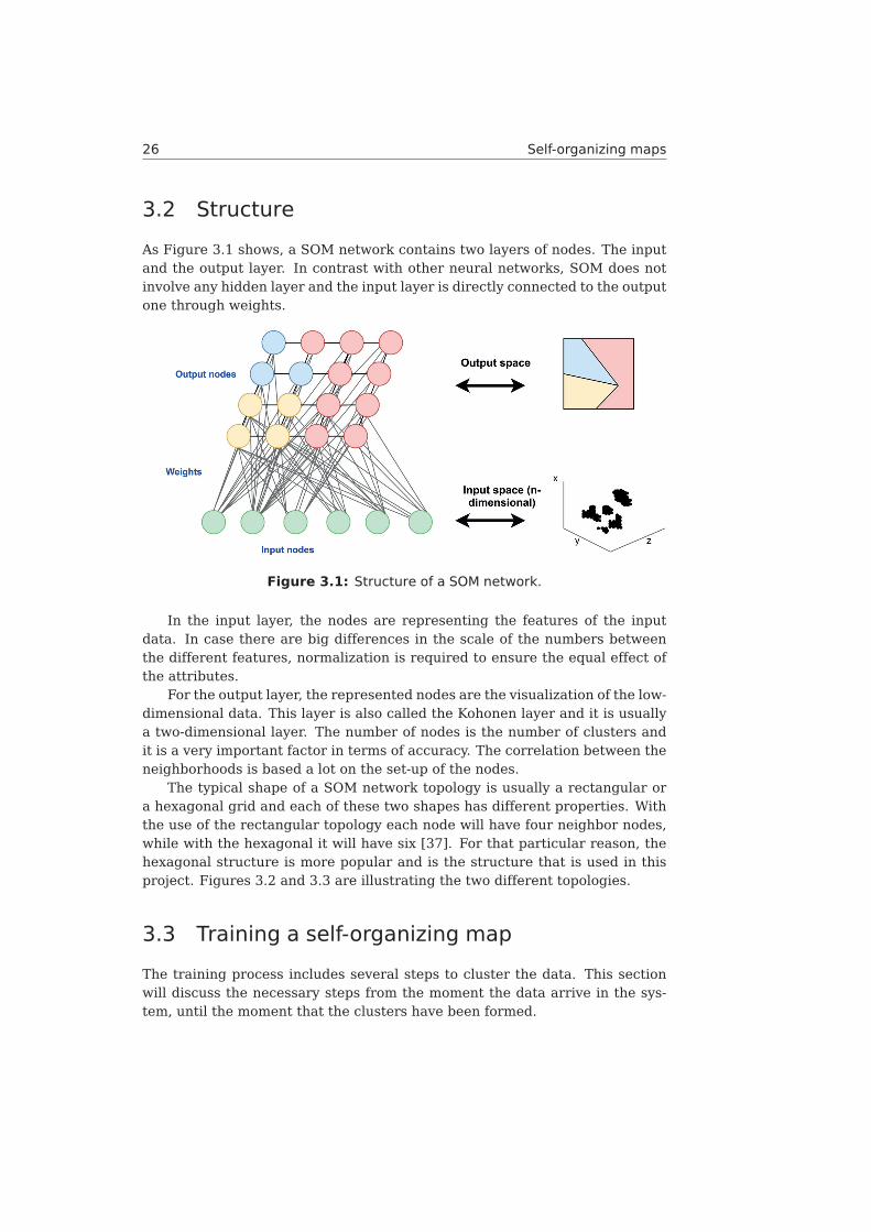
As Figure 3.1 shows, a SOM network contains two layers of nodes. The inputand the output layer. In contrast with other neural networks, SOM does notinvolve any hidden layer and the input layer is directly connected to the outputone through weights.
Figure 3.1: Structure of a SOM network.
In the input layer, the nodes are representing the features of the inputdata. In case there are big differences in the scale of the numbers betweenthe different features, normalization is required to ensure the equal effect ofthe attributes.
For the output layer, the represented nodes are the visualization of the low-dimensional data. This layer is also called the Kohonen layer and it is usuallya two-dimensional layer. The number of nodes is the number of clusters andit is a very important factor in terms of accuracy. The correlation between theneighborhoods is based a lot on the set-up of the nodes.
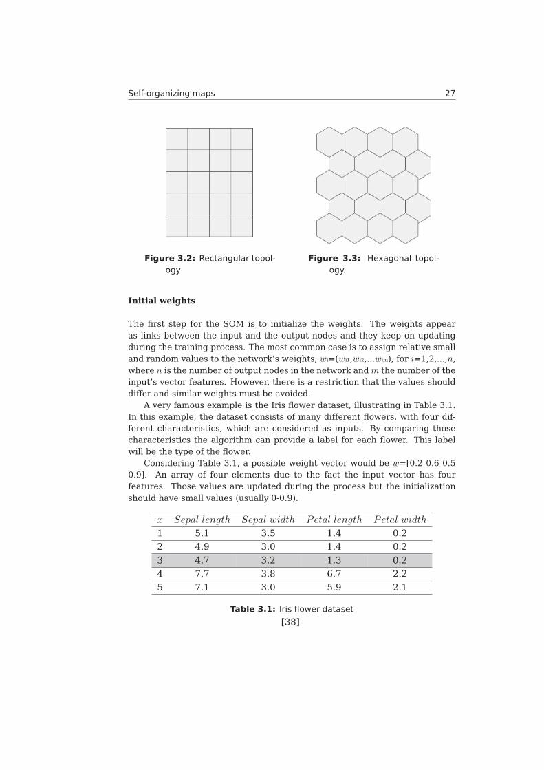
The typical shape of a SOM network topology is usually a rectangular ora hexagonal grid and each of these two shapes has different properties. Withthe use of the rectangular topology each node will have four neighbor nodes,while with the hexagonal it will have six [37]. For that particular reason, thehexagonal structure is more popular and is the structure that is used in thisproject. Figures 3.2 and 3.3 are illustrating the two different topologies.
3.3 Training a self-organizing map
The training process includes several steps to cluster the data. This sectionwill discuss the necessary steps from the moment the data arrive in the sys-tem, until the moment that the clusters have been formed.
Self-organizing maps 27
Figure 3.2: Rectangular topol-ogy
Figure 3.3: Hexagonal topol-ogy.
Initial weights
The first step for the SOM is to initialize the weights. The weights appearas links between the input and the output nodes and they keep on updatingduring the training process. The most common case is to assign relative smalland random values to the network’s weights, wi=(wi1,wi2,...wim), for i=1,2,...,n,where n is the number of output nodes in the network andm the number of theinput’s vector features. However, there is a restriction that the values shoulddiffer and similar weights must be avoided.
A very famous example is the Iris flower dataset, illustrating in Table 3.1.In this example, the dataset consists of many different flowers, with four dif-ferent characteristics, which are considered as inputs. By comparing thosecharacteristics the algorithm can provide a label for each flower. This labelwill be the type of the flower.
Considering Table 3.1, a possible weight vector would be w=[0.2 0.6 0.50.9]. An array of four elements due to the fact the input vector has fourfeatures. Those values are updated during the process but the initializationshould have small values (usually 0-0.9).
x Sepal length Sepal width Petal length Petal width
1 5.1 3.5 1.4 0.2
2 4.9 3.0 1.4 0.2
3 4.7 3.2 1.3 0.2
4 7.7 3.8 6.7 2.2
5 7.1 3.0 5.9 2.1
Table 3.1: Iris flower dataset
[38]
28 Self-organizing maps
Sampling
Select randomly input samples from the input space (training data set). Forexample, considering Table 3.1 and the Iris flower dataset, each flower (orsample x) has four different features. In the sampling step for this scenariosample x3, marked as gray, is chosen as a random sample.
Similarity matching
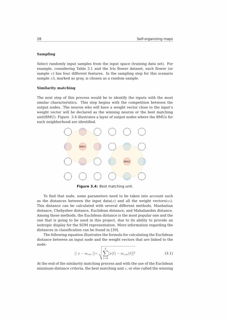
The next step of this process would be to identify the inputs with the mostsimilar characteristics. This step begins with the competition between theoutput nodes. The neuron who will have a weight vector close to the input’sweight vector will be declared as the winning neuron or the best matchingunit(BMU). Figure 3.4 illustrates a layer of output nodes where the BMUs foreach neighborhood are identified.
Figure 3.4: Best matching unit.
To find that node, some parameters need to be taken into account suchas the distances between the input data(x) and all the weight vectors(wi).This distance can be calculated with several different methods, Manhattandistance, Chebyshev distance, Euclidean distance, and Mahalanobis distance.Among those methods, the Euclidean distance is the most popular one and theone that is going to be used in this project, due to its ability to provide anisotropic display for the SOM representation. More information regarding thedistances in classification can be found in [39].
The following equation illustrates the formula for calculating the Euclideandistance between an input node and the weight vectors that are linked to thenode:
|| x− wim ||=√√√√ T∑
t=0
[x(t)− wi,m(t)]2 (3.1)
At the end of the similarity matching process and with the use of the Euclideanminimum-distance criteria, the best matching unit c, or else called the winning
Self-organizing maps 29
neuron, is detected after some iterations with the above equation:
c(t) = min(|| x− wim ||) = min(
√√√√ T∑t=0
[x(t)− wi,m(t)]2) (3.2)
where T is the maximum number of iterations that the network will perform.
Neighborhood function
The neighborhood function is responsible for providing a relation between asample and its neighbors, as well as the topological order of the map. In casethat this function is missing then the SOMs are the same with the k-means al-gorithm, which is an algorithm more based on averaging the selected sampleaccording to its neighbor samples. In contrast, SOMs are trying to match theselected sample with its closest neighbor and increase the distance with therest of the neighbors. The two most popular functions for this purpose are theGaussian (3.3) and the square function (3.4) :
hg(wij , wmn, r) = exp(− (i− n)2 − (j −m)2
2r2) (3.3)
hs(wij , wmn, r) =
{1 <=
√(i− n)2 + (j −m)2 ≤ r,
0 <=√
(i− n)2 + (j −m)2 > r.(3.4)
Where wij is the selected neuron in position i,j, wmn the neighbor neuron inposition m,n and r is the radius. In both functions, the radius r is decreasingto 0 or 1 during the training. The Gaussian neighborhood is considered as amore reliable solution when the square function requires less computations[40].
For this experiment, the Gaussian neighborhood function was used to ob-tain more accurate outputs.
Weight updating
After identifying the best matching units, their weights and the weights oftheir neighbor units are adjusted to become correlated to the input space fea-tures. The learning rate and the neighborhood size are the two most importantcharacteristics of this weight update.
The learning rate is in charge of the change on the weights and its valuecan differ from 0 to 1. However, the learning rate for the self-organizing mapsis not a stable variable and it is gradually decreasing as the number of itera-tions of the SOMs algorithm is increasing. This decrement can occur linearly,exponentially or inversely proportional to the iterations. In most of the neuralnetwork cases, the weights are assigned randomly and the learning rate startsfrom a very high value, close to 1 and reduces through the time. At the begin-ning of the training, more iterations are occurring, and they are reducing as
30 Self-organizing maps
the process goes on, as there are fewer necessary corrections that need to bedone.
The following formula indicates the updated weight vector wi(t+1) of thewinning neuron and all the neurons that lie in the neighborhood of it, with re-spect to the number of iterations (t), the learning rate (α) and the past weightvector wi(t) :
wi(t+ 1) = wi(t) + α(t)h(wbmu, wi, r)[x(t)− wi(t)] (3.5)
Where h is the neighborhood function, wbmu the weight vector of the bestmatching unit and r the radius of the formed neighborhood [41].
3.4 K-nearest neighbors
The k-Nearest-Neighbors or KNN is considered as one of the simplest algo-rithms for classification and regression. The main function of this algorithm isclassifying input data into outputs by identifying the most common character-istics on them and applying a new set of data from the same type to performpredictions about their outputs. The same approach applies to regression,where the algorithm predicts target values for new data [42].
In contrast with other algorithms, KNN is not using any training method.Instead of that, the moment the input data are available they are classified andafter that, any possible training is applied. However, to perform classification,the algorithm has to go through all the data points. This process makes thisalgorithm very expensive in terms of computation.
The process will follow the below steps :
• Calculate the distance between the selected input value (a random valuefrom the training dataset) and the rest of the training data inputs.
• Choose k amount of data points, located close to the selected data point.Those points are identified as the ones with the lowest distance values.
• Evaluate according to their distance value and the number of similardata in each class, to which class the selected data point will be classi-fied (or in case of regression what would be the predicted value) for therest of the data.
There are two factors to be taken under consideration before the KNNprocess starts. The first one is the value of k, which can just be a randomnumber or a fixed one after tests and optimizations. For this project k was setas 3, since that was the number that provided the most accurate results.
The second one would be the distance metric that the algorithm is going touse. As it was mentioned before for SOMs, there are many different methodsfor calculating this distance for KNN. Likewise SOMs, the Euclidean distanceis the most popular one, which is described in the previous section and the
Self-organizing maps 31
one that is used in the KNN model of this work. Equation 3.1 will be appliedfor the case of the KNN as well [43].
To summarize the KNN model includes the following steps:
• The load of the data.
• The initialization of the value for the k factor.
• Multiple iterations for each data in order to obtain the predicted class.
In the last step, the algorithm first calculates the distance between the testand each of the training data. Then according to the calculated distances thek top distances (the ones with the lowest values) will be selected. The mostfrequent class label among those elements will be obtained and assigned asthe predicted class.
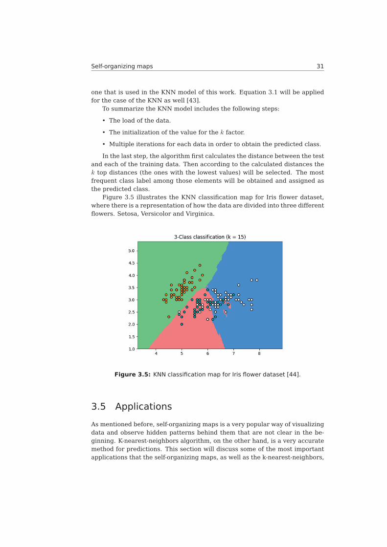
Figure 3.5 illustrates the KNN classification map for Iris flower dataset,where there is a representation of how the data are divided into three differentflowers. Setosa, Versicolor and Virginica.
Figure 3.5: KNN classification map for Iris flower dataset [44].
3.5 Applications
As mentioned before, self-organizing maps is a very popular way of visualizingdata and observe hidden patterns behind them that are not clear in the be-ginning. K-nearest-neighbors algorithm, on the other hand, is a very accuratemethod for predictions. This section will discuss some of the most importantapplications that the self-organizing maps, as well as the k-nearest-neighbors,
32 Self-organizing maps
are involved too.
Applications of self-organizing maps
One very interesting research has been published by Ryotaro Kamimura (2012),where SOMs is used as an algorithm for analyzing data for automobile indus-tries in Japan and predict the financial state of the country since researcheshave proved that those data are related and affect the country’s economy [45].
Another important application has been released by Suzanne Angeli et. al(2012). This study is investigating the classification of earth observation datawith the use of self-organizing maps. Those data are from sensors on earththat are monitoring the atmosphere and some geophysical properties such asidentifying the clouds or the areas that are covered by ice. To receive thatinformation, there is a need for pixel processing for the obtained picture froma satellite. The conventional approach to this is with the use of decision trees,but this research replaces the decision tree solution with the self-organizingmaps. The results are indicating that SOM is a very effective algorithm forthis application and it is providing a simpler solution to the problem [46].
At last, an interesting approach within the financial sector has been pub-lished by Li Jian et. al (2016). Due to the increase of fraudulent financialreporting over the last years, it has been observed that many reports containovervalued profits, sales, and assets, or understating liabilities and expenses.Those fault reported values can be usually observed through the financial ra-tios. The financial ratios are mainly divided into two groups, normal and ab-normal group and the fraudulent data are mostly located into the abnormalgroup. As a result, the SOMs are classifying the input data into two individ-ual classes. The results are showing that SOMs are effective in detecting thefraudulent financial data with high accuracy however the results could be fur-ther improved by enlarging the dataset or by trying and comparing differentunsupervised algorithms [47].
Applications of k-nearest neighbors
KNN algorithm is very popular as a text mining technique with a wide va-riety of applications. In their paper Suhatati Tjandral et. al (2015), theyare examining the use of the KNN as a text mining algorithm where the fi-nal design is used as a system by the government to receive complaints fromthe citizens. With the use of its data mining properties, KNN can detect thedepartment that should receive the complaint text and the mail is being for-warded to them. As was expected the results showed that KNN can be usedas a very reliable text mining system [48].
Facial image analysis is considered as a very important part of the imageprocessing area. It can be used for face recognition, psychological tests, andseveral more applications. Treesa George et. al (2014), in their research, ex-plore the application of the KNN algorithm for the detection of a smile within
Self-organizing maps 33
still images. With the use of another classification algorithm called Haar cas-cade, the necessary information to detect a mouth and a pair of eyes on a faceare extracted. Then those values are provided as input training data to theKNN algorithm. The results are showing that with the use of the mouth onlythe accuracy is 60% but including the eye pair as well the result is increasingand the algorithm becomes more accurate [49].
Finally, an interesting research paper is published from S.Venkata Lakshmiand T.Edwin Prabakaran (2014), where with the use of the KNN they are de-tecting cyber-attacks to a network, by examining some specific features andlooking for potential intrusions. The data for train and testing are provided bythe KDD Cup dataset, which is considered as the benchmark data in Intrusiondetection and contains 41 different features for each data. By changing thenumber and the type of features within 5 sets, different threats can be iden-tified. Set five appeared to be the most effective since the biggest amount ofthreats was identified with the use of those features while it had less amountof data compared to other datasets [50].
Combining self-organizing maps with k-nearest neighbors
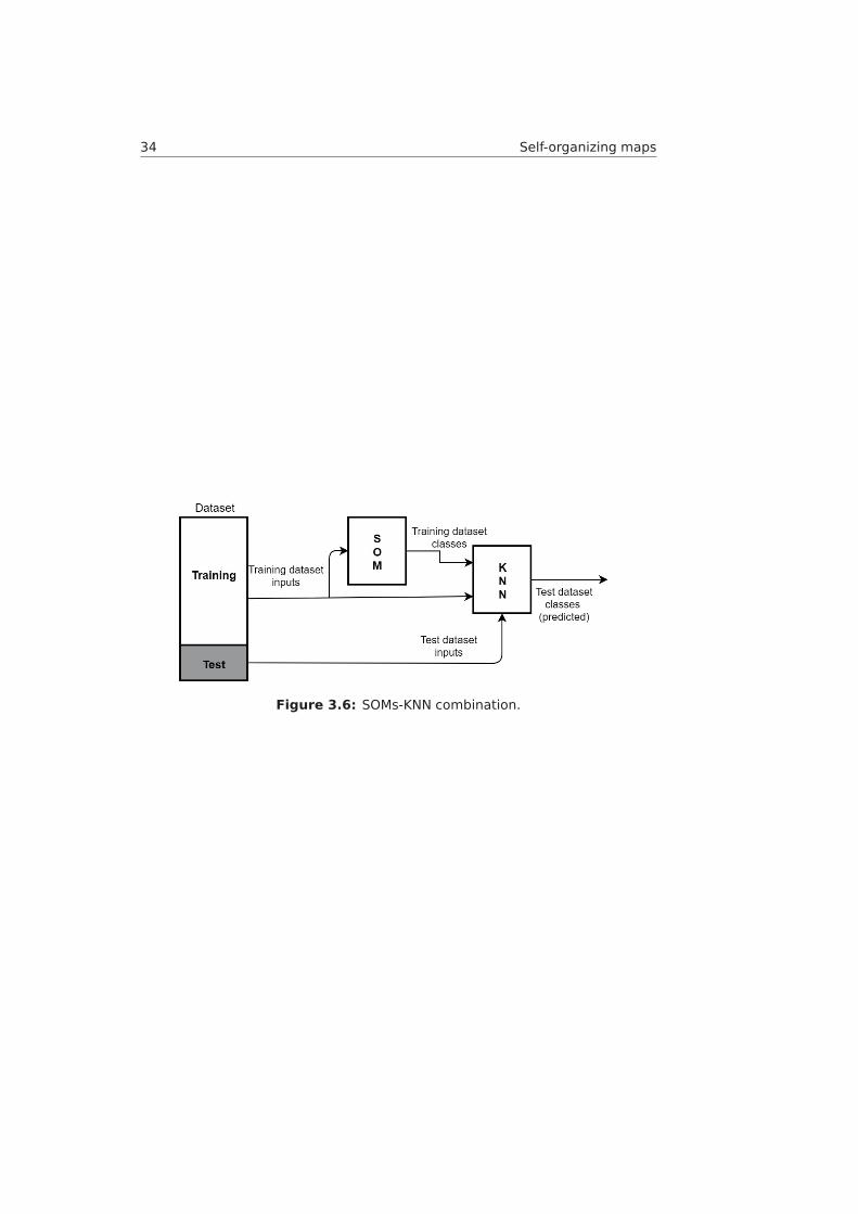
The two algorithms described before in the chapter, self-organizing maps (SOMs)and k-Nearest-Neighbors (KNN), are combined in this project to provide a finalresult and replace the conventional approach for the digital pre-distortion.
The self-organizing maps are used as a mean of classification. In otherwords, this algorithm is used to obtain a class value (label) by identifying thecommon characteristics among the input data. This, however, is applied onlyto a part of the input dataset. This dataset is called the training dataset.
The k-Nearest-Neighbors, on the other hand, are used as a mean of re-gression. Using the training dataset in combination with their class values,the algorithm can perform a class prediction for the rest of the data (calledtest set) by providing their input values.
Figure 3.6 illustrates a simple representation of the two algorithms com-bined. The next chapter will explain more in-depth how this concept is appliedto the design.
34 Self-organizing maps
Figure 3.6: SOMs-KNN combination.
Chapter4Implementation and results
This chapter will discuss the approach for the neural network based DPD de-sign, the architecture that was used and the given results. The simulationswere executed with the use ofMATLAB and the algorithm was developed withMATLAB’s neural network toolbox. Some additional simulations for calcu-lating the computational complexity were executed with the use of Pythonscripts.
4.1 Specifications
According to the current industry’s needs and to the 3GPP specifications, aproper EVM for a base station should be below 8% [51]. However, the PA isonly a part of the base station and there are other components in the systemsuch as the modulators and the RF transceivers that are affecting the totalEVM. For this reason, EVM just for the PA should be in lower levels, around4% or even less.
On the other hand, the ACPR of the conventional approach is around -45dBc which is considered as a very good and low ACPR. According to thepredicted performance losses, and the 5G NR specifications [52], an ACPRvalue for a PA with a channel offset of 400MHz, as the one used in this project,would be between -27dBc and -33dBc.
4.2 The concept
As it was shown in Figure 2.6, in the LUT-based model there are many differentLUTs according to the system’s memory taps. The idea of this project is toprove that all those LUTs could be replaced by just one that will use the inputx as an index and predict the y value (instead of (2.5)). Input x refers to thepre-distorter’s input and y to the pre-distorter’s output (for more details checksection 2.2 and 2.4). This implementation can reduce the required amount of
35
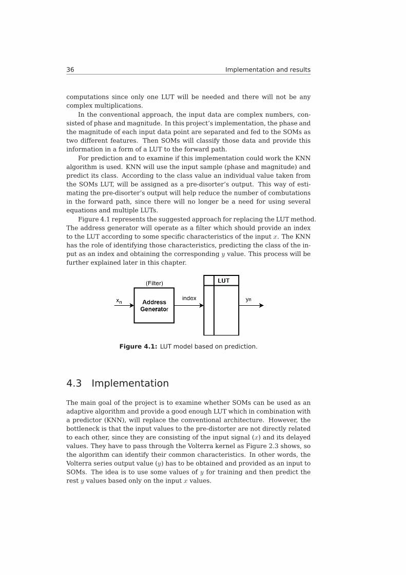
36 Implementation and results
computations since only one LUT will be needed and there will not be anycomplex multiplications.
In the conventional approach, the input data are complex numbers, con-sisted of phase and magnitude. In this project’s implementation, the phase andthe magnitude of each input data point are separated and fed to the SOMs astwo different features. Then SOMs will classify those data and provide thisinformation in a form of a LUT to the forward path.
For prediction and to examine if this implementation could work the KNNalgorithm is used. KNN will use the input sample (phase and magnitude) andpredict its class. According to the class value an individual value taken fromthe SOMs LUT, will be assigned as a pre-disorter’s output. This way of esti-mating the pre-disorter’s output will help reduce the number of combutationsin the forward path, since there will no longer be a need for using severalequations and multiple LUTs.
Figure 4.1 represents the suggested approach for replacing the LUTmethod.The address generator will operate as a filter which should provide an indexto the LUT according to some specific characteristics of the input x. The KNNhas the role of identifying those characteristics, predicting the class of the in-put as an index and obtaining the corresponding y value. This process will befurther explained later in this chapter.
Figure 4.1: LUT model based on prediction.
4.3 Implementation
The main goal of the project is to examine whether SOMs can be used as anadaptive algorithm and provide a good enough LUT which in combination witha predictor (KNN), will replace the conventional architecture. However, thebottleneck is that the input values to the pre-distorter are not directly relatedto each other, since they are consisting of the input signal (x) and its delayedvalues. They have to pass through the Volterra kernel as Figure 2.3 shows, sothe algorithm can identify their common characteristics. In other words, theVolterra series output value (y) has to be obtained and provided as an input toSOMs. The idea is to use some values of y for training and then predict therest y values based only on the input x values.
Implementation and results 37
The data set is split into two parts. The first one is the training set, whichincludes a part of the pre-distorter’s inputs. Those values are going to beconsidered as the input values for the training (i.e the first 40% of the pre-distorter’s input values). The second one is the test set, which will containa part of the rest of the pre-distorter’s input values (i.e the last 20% of theinput values). This set will be used as input to the KNN and the algorithmwill predict its outputs. The performance and accuracy of those results will bemeasured with the use of ACPR and EVM respectively and the computationalcomplexity by measuring the floating point operations (FLOP).
4.3.1 Training stage
For this project, the two feature input to SOMs will be the phase and the mag-nitude of y, which is obtained by splitting the real and the imaginary part ofthis complex value. When the values of y pass into the SOMs, then the neuralnetwork will divide them into classes by identifying their common character-istics, as it was explained in Chapter 3.
The next step will be to estimate an average y value for each class andstore it into a table. With this step the average y could be used instead ofthe original one for each input value, resulting in a significant decrease of thedifferent y values. At the end of this process, each class will have a unique y
value.
For example for a dataset of 100000 different values of x corresponding to100000 different values of y, applying this implementation using 1000 classescan reduce the number of y values from 100000 to just 1000 values, a decreaseof 99%. Of course, the main drawback of this implementation will be the lossin accuracy and that is a part of what this thesis is investigating.
Figure 4.2 illustrates how the above process is implemented in the system.This part is the training stage where the data are trained in order to providethe system with the required information for the processing stage, where theprediction is taking place.
It is worth to be mentioned that the conventional approach with the useof LUTs (Figure 2.6) will run for several iterations (5 in this project) in orderfor the coefficients to get updated and provide a more accurate result for y.The coefficients will have random values from 0 to 1 at the beginning of theprocess and they will be updated after each iteration through the equation(2.4). This process will occur only for the training set.
4.3.2 Processing stage
After each input x of the training dataset has a class and a y (average) value,the following step will be to provide this information to the KNN algorithm inorder to predict classes for the test set. Now the test set consists of x values aswell, since the initial dataset was split into two separate datasets. The training

38 Implementation and results
Figure 4.2: Training stage, classification of the input values.
dataset and the test dataset. After the KNN predicts a class for each of thetest set value, then the corresponding y for each class will be assigned, as itwas estimated in the training set. Of course, it is important that the trainingstage and the processing stage are using the same amount of classes so it ispossible to find an average y value for each class after the KNN predicts aclass value. By using fewer classes, for both testing and processing stage, theshrinking of the original amount of values can be achieved but this will lead toa decrease in the system’s accuracy.
Figure 4.3 represents how the class prediction for the test data is exe-cuted.
Figure 4.3: Processing stage, prediction of the output.
By providing the input x of the training set and their class values, theKNN can predict a class value for each of the test set values. This is achievedby finding the closest neighbors to the value or in other words the closestmatching classes. This closest matching class will be the predicted class.
After the KNN has predicted a class value for each test data x, this classwill be used as an index to the LUT (Training data table) to obtain the y (av-
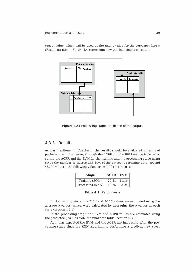
Implementation and results 39
erage) value, which will be used as the final y value for the corresponding x
(Final data table). Figure 4.4 represents how this indexing is executed.
Figure 4.4: Processing stage, prediction of the output.
4.3.3 Results
As was mentioned in Chapter 2, the results should be evaluated in terms ofperformance and accuracy through the ACPR and the EVM respectively. Mea-suring the ACPR and the EVM for the training and the processing stage using50 as the number of classes and 40% of the dataset as training data (around45000 values), the following values from Table 4.1 resulted.
Stage ACPR EVM
Training (SOM) -20.51 21.10Processing (KNN) -19.85 23.25
Table 4.1: Performance
In the training stage, the EVM and ACPR values are estimated using theaverage y values, which were calculated by averaging the y values in eachclass (section 4.3.1).
In the processing stage, the EVM and ACPR values are estimated usingthe predicted y values from the final data table (section 4.3.2).
As it was expected the EVM and the ACPR are increasing after the pro-cessing stage since the KNN algorithm is performing a prediction so a loss
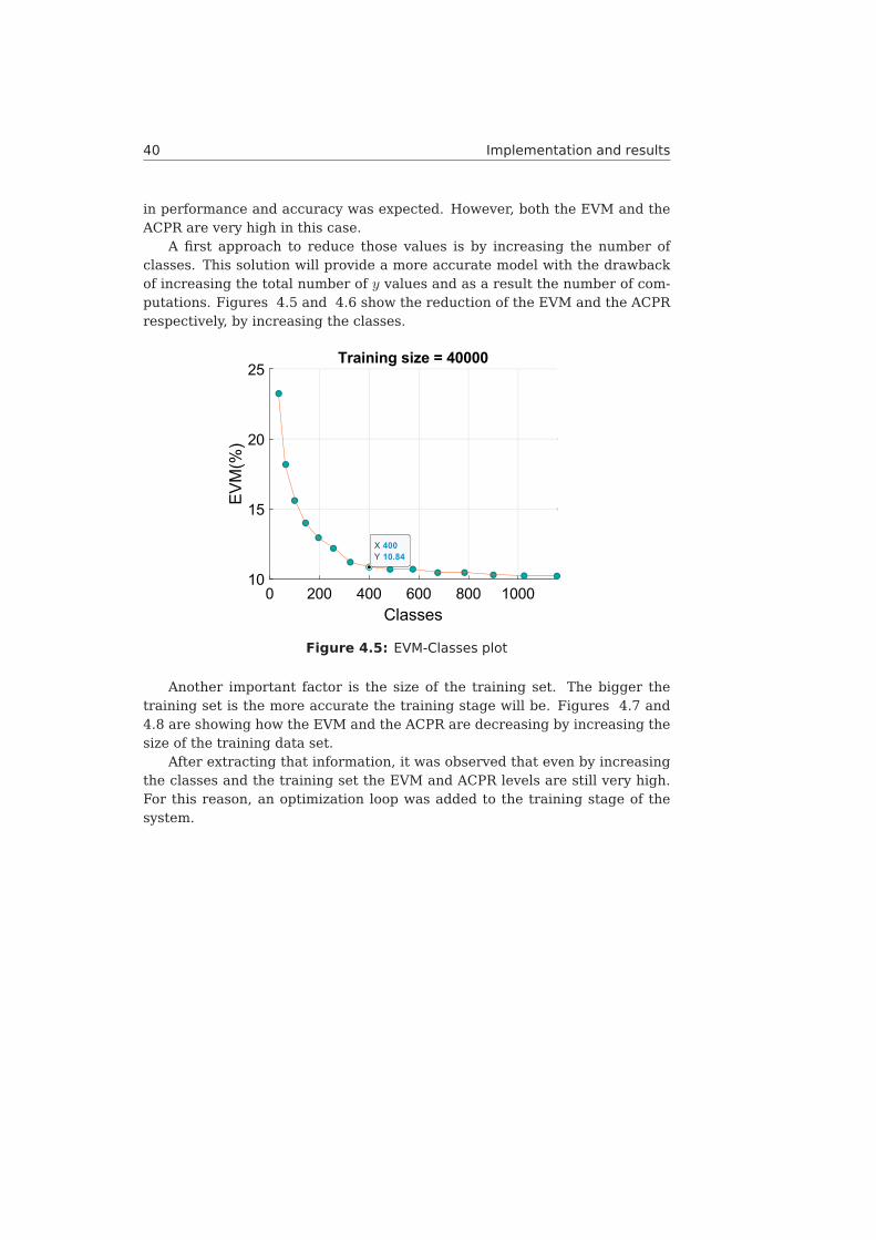
40 Implementation and results
in performance and accuracy was expected. However, both the EVM and theACPR are very high in this case.
A first approach to reduce those values is by increasing the number ofclasses. This solution will provide a more accurate model with the drawbackof increasing the total number of y values and as a result the number of com-putations. Figures 4.5 and 4.6 show the reduction of the EVM and the ACPRrespectively, by increasing the classes.
Figure 4.5: EVM-Classes plot
Another important factor is the size of the training set. The bigger thetraining set is the more accurate the training stage will be. Figures 4.7 and4.8 are showing how the EVM and the ACPR are decreasing by increasing thesize of the training data set.
After extracting that information, it was observed that even by increasingthe classes and the training set the EVM and ACPR levels are still very high.For this reason, an optimization loop was added to the training stage of thesystem.
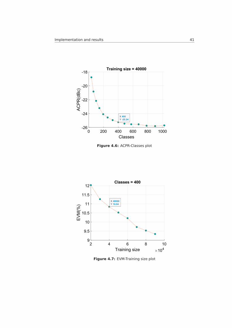
Implementation and results 41
Figure 4.6: ACPR-Classes plot
Figure 4.7: EVM-Training size plot
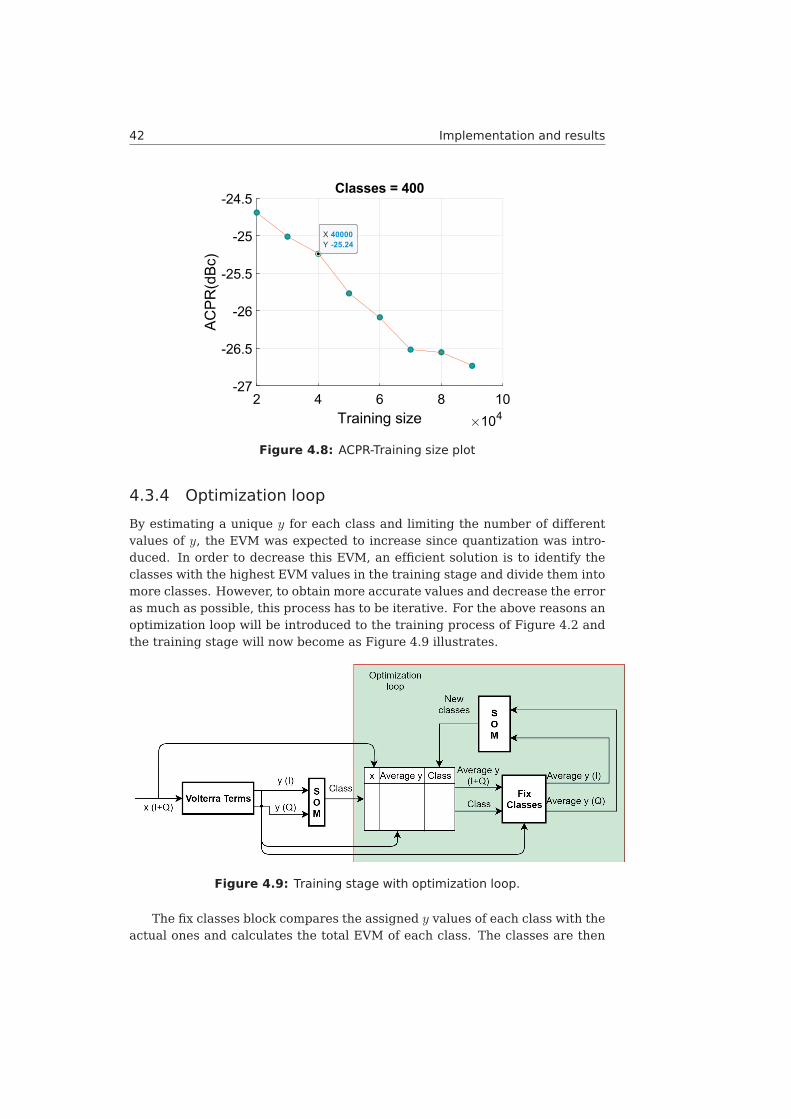
42 Implementation and results
Figure 4.8: ACPR-Training size plot
4.3.4 Optimization loop
By estimating a unique y for each class and limiting the number of differentvalues of y, the EVM was expected to increase since quantization was intro-duced. In order to decrease this EVM, an efficient solution is to identify theclasses with the highest EVM values in the training stage and divide them intomore classes. However, to obtain more accurate values and decrease the erroras much as possible, this process has to be iterative. For the above reasons anoptimization loop will be introduced to the training process of Figure 4.2 andthe training stage will now become as Figure 4.9 illustrates.
Figure 4.9: Training stage with optimization loop.
The fix classes block compares the assigned y values of each class with theactual ones and calculates the total EVM of each class. The classes are then
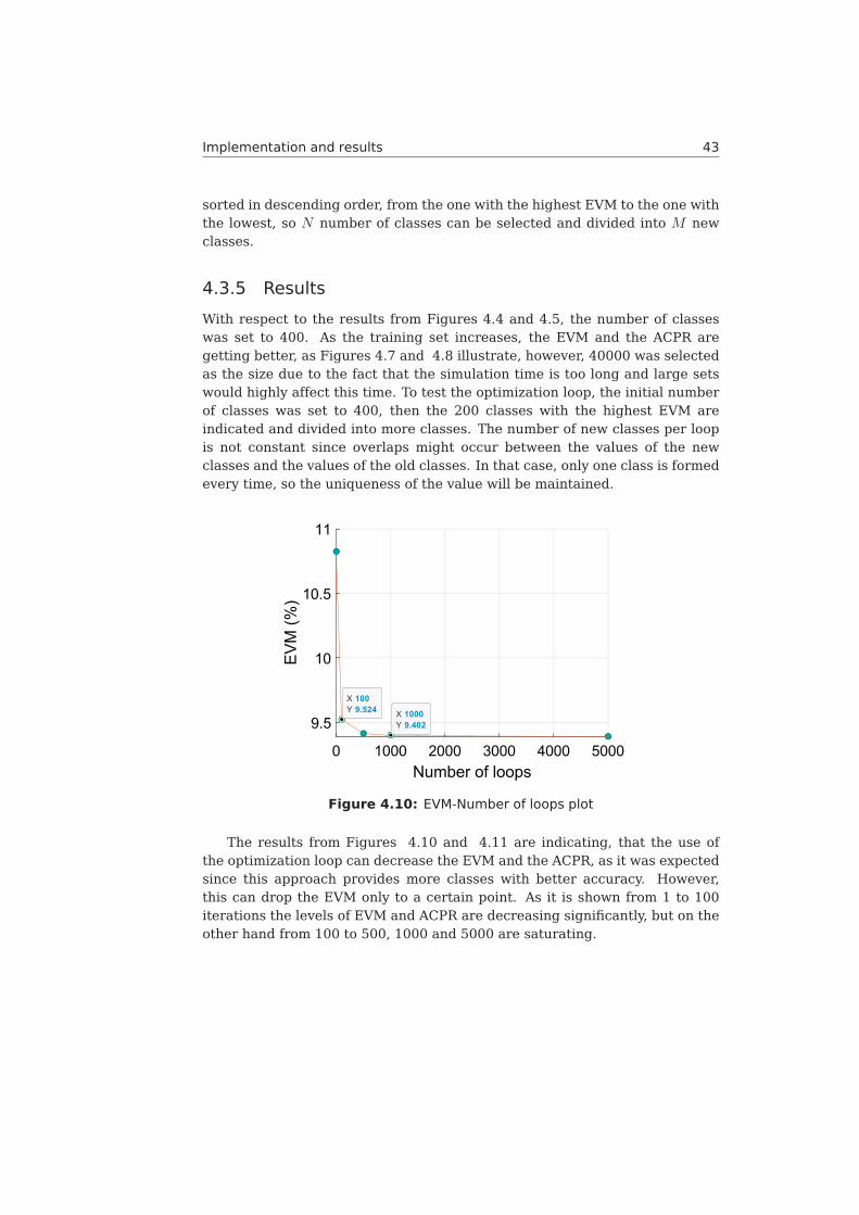
Implementation and results 43
sorted in descending order, from the one with the highest EVM to the one withthe lowest, so N number of classes can be selected and divided into M newclasses.
4.3.5 Results
With respect to the results from Figures 4.4 and 4.5, the number of classeswas set to 400. As the training set increases, the EVM and the ACPR aregetting better, as Figures 4.7 and 4.8 illustrate, however, 40000 was selectedas the size due to the fact that the simulation time is too long and large setswould highly affect this time. To test the optimization loop, the initial numberof classes was set to 400, then the 200 classes with the highest EVM areindicated and divided into more classes. The number of new classes per loopis not constant since overlaps might occur between the values of the newclasses and the values of the old classes. In that case, only one class is formedevery time, so the uniqueness of the value will be maintained.
Figure 4.10: EVM-Number of loops plot
The results from Figures 4.10 and 4.11 are indicating, that the use ofthe optimization loop can decrease the EVM and the ACPR, as it was expectedsince this approach provides more classes with better accuracy. However,this can drop the EVM only to a certain point. As it is shown from 1 to 100iterations the levels of EVM and ACPR are decreasing significantly, but on theother hand from 100 to 500, 1000 and 5000 are saturating.
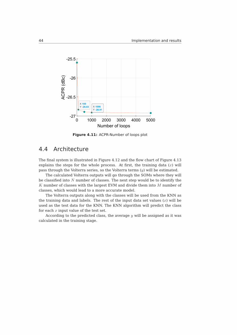
44 Implementation and results
Figure 4.11: ACPR-Number of loops plot
4.4 Architecture
The final system is illustrated in Figure 4.12 and the flow chart of Figure 4.13explains the steps for the whole process. At first, the training data (x) willpass through the Volterra series, so the Volterra terms (y) will be estimated.
The calculated Volterra outputs will go through the SOMs where they willbe classified into N number of classes. The next step would be to identify theK number of classes with the largest EVM and divide them into M number ofclasses, which would lead to a more accurate model.
The Volterra outputs along with the classes will be used from the KNN asthe training data and labels. The rest of the input data set values (x) will beused as the test data for the KNN. The KNN algorithm will predict the classfor each x input value of the test set.
According to the predicted class, the average y will be assigned as it wascalculated in the training stage.
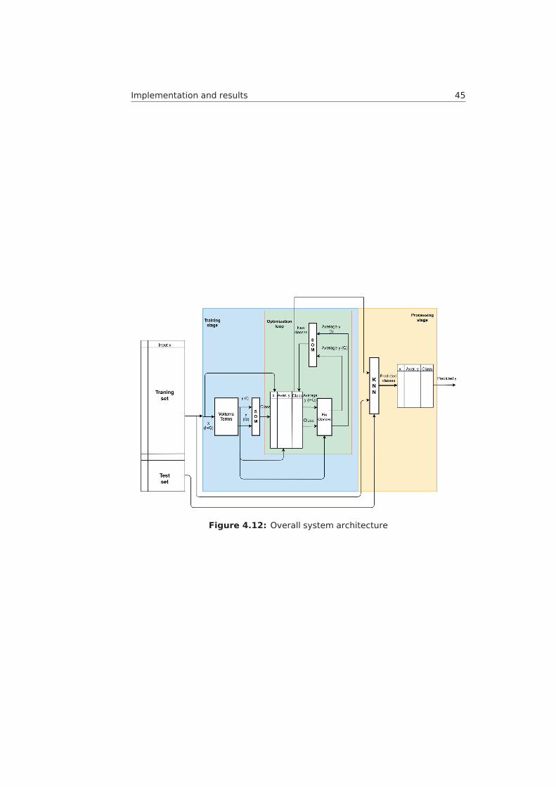
Implementation and results 45
Figure 4.12: Overall system architecture
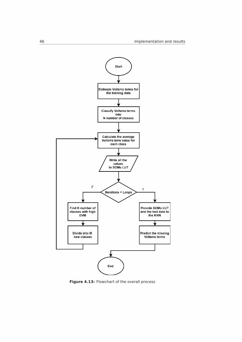
46 Implementation and results
Figure 4.13: Flowchart of the overall process
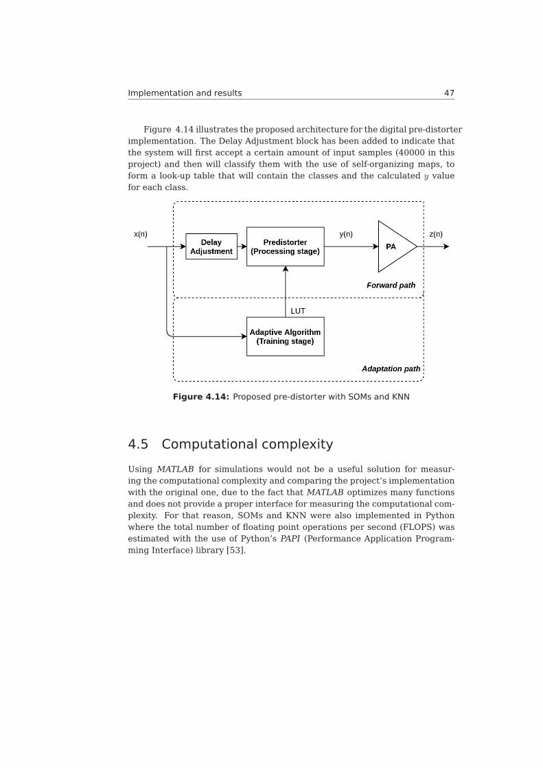
Implementation and results 47
Figure 4.14 illustrates the proposed architecture for the digital pre-distorterimplementation. The Delay Adjustment block has been added to indicate thatthe system will first accept a certain amount of input samples (40000 in thisproject) and then will classify them with the use of self-organizing maps, toform a look-up table that will contain the classes and the calculated y valuefor each class.
Figure 4.14: Proposed pre-distorter with SOMs and KNN
4.5 Computational complexity
Using MATLAB for simulations would not be a useful solution for measur-ing the computational complexity and comparing the project’s implementationwith the original one, due to the fact that MATLAB optimizes many functionsand does not provide a proper interface for measuring the computational com-plexity. For that reason, SOMs and KNN were also implemented in Pythonwhere the total number of floating point operations per second (FLOPS) wasestimated with the use of Python’s PAPI (Performance Application Program-ming Interface) library [53].
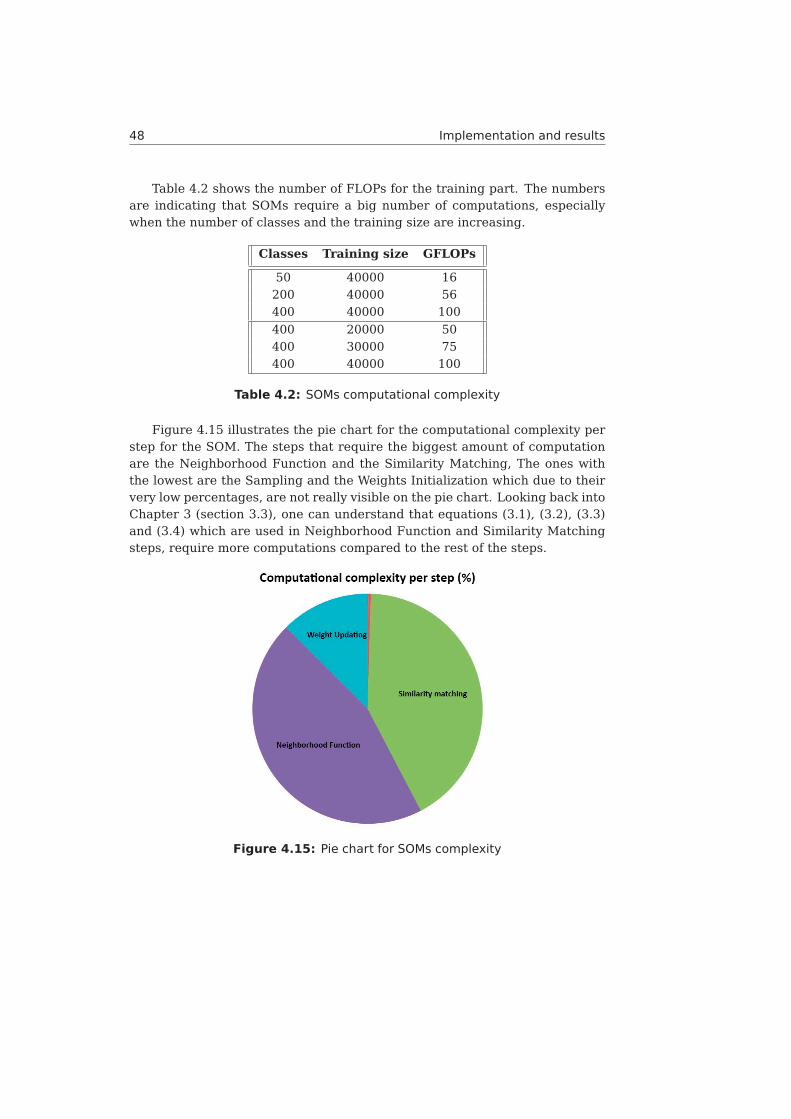
48 Implementation and results
Table 4.2 shows the number of FLOPs for the training part. The numbersare indicating that SOMs require a big number of computations, especiallywhen the number of classes and the training size are increasing.
Classes Training size GFLOPs
50 40000 16200 40000 56400 40000 100
400 20000 50400 30000 75400 40000 100
Table 4.2: SOMs computational complexity
Figure 4.15 illustrates the pie chart for the computational complexity perstep for the SOM. The steps that require the biggest amount of computationare the Neighborhood Function and the Similarity Matching, The ones withthe lowest are the Sampling and the Weights Initialization which due to theirvery low percentages, are not really visible on the pie chart. Looking back intoChapter 3 (section 3.3), one can understand that equations (3.1), (3.2), (3.3)and (3.4) which are used in Neighborhood Function and Similarity Matchingsteps, require more computations compared to the rest of the steps.
Figure 4.15: Pie chart for SOMs complexity
Implementation and results 49
Classes Training size MFLOP/sample EVM(%) ACPR(dBc)
50 40000 14.2 18.3 -20.8200 40000 13.9 12.6 -24.2400 40000 14.7 10.8 -25.2
400 20000 8.7 12 -24.74400 30000 11.5 11.25 -25.22400 40000 14.7 10.8 -25.2
Table 4.3: KNN computational complexity
Table 4.3 illustrates the computational complexity of the KNN pre-distorter.As the results are showing, there is no difference on the amount of computa-tions when the number of classes is increased. However, this is not the caseabout the training size. As it was expected the training size affects the amountof computations, since the KNN algorithm compares its input sample with allthe values of the training set. The number of classes will not affect that com-parison since it will always be one feature, but with different range of valuesdepending on the total classes. In contrast, increasing the training size willincrease the number of samples that will have to be compared with the KNN’sinput size and it is easy to understand that this will affect the computations.
4.6 Comparison to the Look-Up Table (LUT) pre-distorter
In the proposed implementation the training part is required to run only onceand form the LUT, that will be provided to the KNN. For that reason the KNNpre-distorter is compared in this section with the LUT approach.
According to Figure 4.10 and 4.11, the best results for the KNN pre-distorter were obtained after the use of the optimization loop. This will requireSOMs to be executed multiple times so the number of computations for thetraining part will increase even more. Since the difference after the first 100iterations was not that big, the KNN pre-distorter results for 100 SOMs opti-mization loops will be used and be compared with the LUT pre-distorter(seeFigure 4.11 and 4.12). The selected training size is 40000 and the total num-ber of classes after 100 loops was around 6000.
The project’s simulation data were taken from a 28GHz band PA, withbandwidth up to 400MHz. The pre-distorter’s memory depth for the LUT im-plementation was 3 and the polynomial order 5.
pre-distorter MFLOP/sample EVM(%) ACPR(dBc)
KNN 14.6 9.5 -26.8
LUT 71 3.8 -45.2
Table 4.4: Summary of KNN and LUT pre-distorter

50 Implementation and results
Observing Table 4.4, one can conclude that the KNN pre-distorter requiresa small amount of computations per sample, compared to the original ap-proach. However, the accuracy and the performance has dropped significantlyand such an implementation would be difficult to meet the industry’s specifi-cations as those mentioned on Section 4.1. The next chapter will focus ondiscussing this projects results and some possible improvements that could bemade to get this design one step closer to the industry’s requirements.
Chapter5Conclusions and future work
5.1 Conclusions
The main goal of this thesis project was to develop an innovative solution fordigital pre-distortion with the use of self-organizing maps and investigate thequality of the results. Using the LUT-based pre-distorter scheme as a baseand a mean of comparison, this implementation is targeting on reducing themultiple LUTs on the forward path with only one that will be formed by SOMsand provided to the KNN algorithm in order to estimate the pre-distortersoutput value. In addition to that, this project’s implementation needs to usethe Memory Polynomial only for a limited amount of data in the beginning ofthe process to form the LUT.
The results are indicating that as it was expected the accuracy of themodel is worse than the conventional one since it is based on predictions.However, in terms of computational complexity the KNN pre-distorter is moreefficient than the LUT pre-distorter for the used PA. This difference can beeven more significant if the KNN pre-distorter is compared with pre-distorterswith higher memory depth and polynomial order due to the fact that in thosecases the FLOPs are increasing in the conventional approach but will not af-fect the forward path of this design. However, it will affect the adaptation pathwith SOMs, which needs to be executed initially to form the LUT.
By investigating further the results, some interesting parts were observedsuch as that the accuracy of the model could be increased by increasing thenumber of classes. A scenario that makes sense. since predicting the output,using a limited number of pre-estimated values, generates some quantizationto the output values which will lead to an increase of the error. In order toaim for the quality and not the quantity of the classes, the optimization loopwas introduced and the error was reduced while the number of classes wasmaintained on a reasonable level. Due to the long simulation time in thisproject not all the possible scenarios and combinations were tested.
The project concludes that theoretically by starting with a small number ofclasses and introducing new classes through the optimization loop, the EVMand the ACPR can reach even lower levels and they might be able to meet
51

52 Conclusions and future work
the specifications. To achieve that more simulations are required, with verylong execution time, which will also lead to an increment in the amount ofcomputations in the adaptation path, since SOMs will be executed more times.
5.2 Future work
As an extension of this thesis, I would like to mention four basic points thatcould be further examined and improved:
• The optimization of the existing system to reach better EVM and ACPRlevels and meet the specifications.
• The replacement of the KNN with a different prediction algorithm thatcould be more accurate and hardware-friendly in terms of computations.
• The hardware implementation of the system and the testing in real-lifescenarios with bigger amount of data.
• A comparison of this design with different pre-distorters with biggermemory depth and polynomial order.

References
53
References
[1] Electronics Hub, What is a Power Amplifier? Types, Classes, Appli-cations, 2018. https://www.electronicshub.org/power-amplifier/#What_is_a_Power_Amplifier
[2] John Price and Terry Goble„ Signals and noise.Elsevier Inc, 1993.
[3] Xilinx, IncUnderstanding Key Parameters for RF-Sampling Data Convert-ers. White Paper: Zynq UltraScale+ RFSoCs, February 20, 2019.
[4] Erik Andersson, Christian Olsson, Linearization of Power Amplifier usingDigital Predistortion, Implementation on FPGA. Department of ElectricalEngineering, Linköpings universitet, Linköping, Sweden, 2014.
[5] Wei Wei, Ole Kiel Jensen, Jan H. Mikkelsen, Self-heating and memoryeffects in RF power amplifiers explained through electrothermal. IEEEPress, Aalborg Universitet, Denmark, 2013.
[6] Christian Henn, Burr-Brown International, GmbH. Intermodulation Dis-tortion (IMD). Burr-Brown International,Texas Instruments Incorpo-rated, Tucson, Arizona, 2000.
[7] Ibrahim Can Sezgin, Different Digital Predistortion Techniques for PowerAmplifier Linearization. Department of Electrical and Information Tech-nology Faculty of Engineering, LTH, Lund, Sweden, 2016.
[8] Aidan Wilson, A Brief Introduction to Supervised Learning. TowardsData Science, September 29, 2019. https://towardsdatascience.com/a-brief-introduction-to-supervised-learning-54a3e3932590
[9] Barber, D, Bayesian Reasoning and Machine Learning. Cambridge Uni-versity Press, 2012.
[10] Nagyfi Richárd. The differences between Artificial and BiologicalNeural Networks. Sep 4, 2018. https://towardsdatascience.com/the-differences-between-artificial-and-biological-neural-networks-a8b46db828b7
54
References 55
[11] Sylvester Kaczmarek, What You Need to Know About Ma-chine Learning. Electronic Design an informa business, 2017.https://www.electronicdesign.com/industrial-automation/what-you-need-know-about-machine-learning
[12] Q.Wu and Z.Ni, Car assembly line fault diagnosis based on triangularfuzzy support vector classifier machine and particle swarm optimization.Expert Syst, 2011.
[13] M. Gardner and J. Bieker, Data mining solves tough semiconductor man-ufacturing problems. In Proc. 6th ACM SIGKDD Conference, 2000.
[14] Darko Stanisavljevic and Michael Spitzer, A Review of Related Work onMachine Learning in Semiconductor Manufacturing and Assembly Lines.SamI40 workshop at i-KNOW’, Graz, Austria, 2016.
[15] A. F. Tabrizi et al. A machine learning framework to identify detailedrouting short violations from a placed netlist. DAC, 2018.
[16] A. F. Tabrizi, N. K. Darav, L. Rakai, A. Kennings, and L. Behjat Detailedrouting violation prediction during placement using machine learning.VLSI-DAT, 2017.
[17] W.-T. J. Chan, P.-H. Ho, A. B. Kahng, and P. Saxena Routability optimiza-tion for industrial designs at sub-14nm process nodes using machinelearning. ISPD, 2017.
[18] Wei Zeng, Azadeh Davoodi, and Yu Hen Hu Design Rule Violation HotspotPrediction Based on Neural Network Ensembles. University of Wiscon-sin–Madison, 2018.
[19] Dennis R. Morgan, Zhengxiang Ma, Jaehyeong Kim, Michael G. Zierdt,and John Pastalan A Generalized Memory Polynomial Model for DigitalPredistortion of RF Power Amplifiers. IEEE Transactions on Signal Pro-cessing, 2006.
[20] Ibrahim Can Sezgin, Different Digital Predistortion Techniques for PowerAmplifier Linearization. Department of Electrical and Information Tech-nology, Faculty of Engineering, LTH, Lund University, 2016.
[21] Henna Paaso and Aarne Mämmelä, Comparison of direct learning andindirect learning predistortion architectures. ISWCS ’08. IEEE, 2008
[22] Takao Inoue, Digital Predistortion (DPD) Design-to-Prototype Frameworkfor PA’s. National Instruments, AWR Corporation, 2013.
[23] F.M Ghannouchi and Oualid Hammi, Behavioral Modeling and Predistor-tion. Microwave Magazine, IEEE, 2010.
[24] Maria Canavate-Sanchez, Andrea Segneri, Apostolos Georgiadis, SavvasKosmopoulos, George Goussetis, Yuan Ding System performance evalua-tion of power amplifier behavioural models. Heriot-Watt University, 2018.
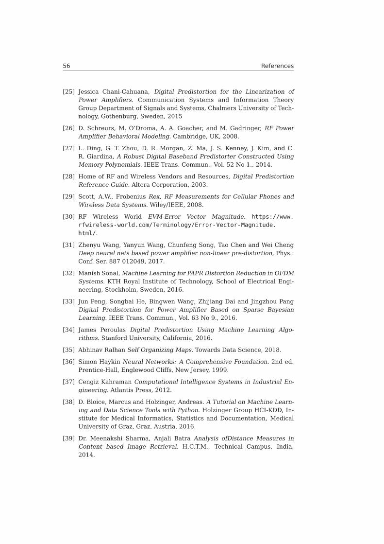
56 References
[25] Jessica Chani-Cahuana, Digital Predistortion for the Linearization ofPower Amplifiers. Communication Systems and Information TheoryGroup Department of Signals and Systems, Chalmers University of Tech-nology, Gothenburg, Sweden, 2015
[26] D. Schreurs, M. O’Droma, A. A. Goacher, and M. Gadringer, RF PowerAmplifier Behavioral Modeling. Cambridge, UK, 2008.
[27] L. Ding, G. T. Zhou, D. R. Morgan, Z. Ma, J. S. Kenney, J. Kim, and C.R. Giardina, A Robust Digital Baseband Predistorter Constructed UsingMemory Polynomials. IEEE Trans. Commun., Vol. 52 No 1., 2014.
[28] Home of RF and Wireless Vendors and Resources, Digital PredistortionReference Guide. Altera Corporation, 2003.
[29] Scott, A.W., Frobenius Rex, RF Measurements for Cellular Phones andWireless Data Systems. Wiley/IEEE, 2008.
[30] RF Wireless World EVM-Error Vector Magnitude. https://www.rfwireless-world.com/Terminology/Error-Vector-Magnitude.html/.
[31] Zhenyu Wang, Yanyun Wang, Chunfeng Song, Tao Chen and Wei ChengDeep neural nets based power amplifier non-linear pre-distortion, Phys.:Conf. Ser. 887 012049, 2017.
[32] Manish Sonal,Machine Learning for PAPR Distortion Reduction in OFDMSystems. KTH Royal Institute of Technology, School of Electrical Engi-neering, Stockholm, Sweden, 2016.
[33] Jun Peng, Songbai He, Bingwen Wang, Zhijiang Dai and Jingzhou PangDigital Predistortion for Power Amplifier Based on Sparse BayesianLearning. IEEE Trans. Commun., Vol. 63 No 9., 2016.
[34] James Peroulas Digital Predistortion Using Machine Learning Algo-rithms. Stanford University, California, 2016.
[35] Abhinav Ralhan Self Organizing Maps. Towards Data Science, 2018.
[36] Simon Haykin Neural Networks: A Comprehensive Foundation. 2nd ed.Prentice-Hall, Englewood Cliffs, New Jersey, 1999.
[37] Cengiz Kahraman Computational Intelligence Systems in Industrial En-gineering. Atlantis Press, 2012.
[38] D. Bloice, Marcus and Holzinger, Andreas. A Tutorial on Machine Learn-ing and Data Science Tools with Python. Holzinger Group HCI-KDD, In-stitute for Medical Informatics, Statistics and Documentation, MedicalUniversity of Graz, Graz, Austria, 2016.
[39] Dr. Meenakshi Sharma, Anjali Batra Analysis ofDistance Measures inContent based Image Retrieval. H.C.T.M., Technical Campus, India,2014.
References 57
[40] Victor J.A.S. Lobo Application of Self-Organizing Maps to the MaritimeEnvironment. Springer, 2009.
[41] Algobeans Self-organizing maps tutorial. Layman Tutorials in analytics,Algobeans.com, November 2, 2017.https://algobeans.com/2017/11/02/self-organizing-map/
[42] Onel Harrison Machine Learning Basics with the K-Nearest NeighborsAlgorithm. Towards Data Science, 2018.
[43] Devin Soni Introduction to k-Nearest-Neighbors. Towards Data Science,March, 12, 2018.https://towardsdatascience.com/introduction-to-k-nearest-neighbors-3b534bb11d26/
[44] Pedregosa, F. et al. Scikit-learn: Machine Learning in Python. JMLR 12,pp. 2825-2830, 2011.https://scikit-learn.org/stable/auto_examples/neighbors/plot_
classification.html/
[45] Ryotaro Kamimura Social Interaction and Self-Organizing Maps. Appli-cations of Self-Organizing Maps, Magnus Johnsson, IntechOpen, 2012.
[46] Suzanne Angeli, Arnaud Quesney and Lydwine Gross Image Simplifica-tion Using Kohonen Maps: Application to Satellite Data for Cloud De-tection and Land Cover Mapping. Applications of Self-Organizing Maps,Magnus Johnsson, IntechOpen, 21 November, 2012.
[47] Li Jian, Yang Ruicheng and Guo Rongrong Self-Organizing Map Methodfor Fraudulent Financial Data Detection. IEEE, 3rd International Confer-ence on Information Science and Control Engineering, 2016.
[48] Suhatati Tjandral, Amelia Alexandra, Putri Warsito and Judi Prajetno Su-giono Determining Citizen Complaints to The Appropriate GovernmentDepartments using KNN Algorithm. IEEE, 13th International Conferenceon ICT and Knowledge Engineering, 2015.
[49] Treesa George, Sumi. P. Potty and Sneha Jose Smile Detection from StillImages Using KNN Algorithm. IEEE, International Conference on Con-trol, Instrumentation, Communication and Computational Technologies(ICCICCT), 2014.
[50] S.Venkata Lakshmi and T.Edwin Prabakaran Application of k-NearestNeighbour Classification Method for Intrusion Detection in NetworkData. IJCA, International Journal of Computer Applications, Volume 97–No.7, July 2014.
[51] Dr. Oliver Werther and Roland Minihold LTE: System Specifications andTheir Impact on RF Base Band Circuits . Rohde Schwarz, 2013.

58 References
[52] Keysight Technologies. 5G NR (New Radio). Technical Overview litera-ture number 5992-2916EN, 2019. https://www.keysight.com/se/en/assets/7018-06127/technical-overviews/5992-2916.pdf/
[53] Fabien Loison, Mathilde Boutigny. PyPAPI’s documentation. Github,2017. https://flozz.github.io/pypapi/
[54] Intg Ckts, Adjacent Channel Power Ratio (ACPR). 2018. http://analog.intgckts.com/adjacent-channel-power-ratio-acpr/

Self-organizing Maps for DigitalPre-distortionMICHAIL ISAAKIDISMASTER´S THESISDEPARTMENT OF ELECTRICAL AND INFORMATION TECHNOLOGYFACULTY OF ENGINEERING | LTH | LUND UNIVERSITY
Printed by Tryckeriet i E-huset, Lund 2020
MIC
HA
IL ISAA
KID
ISSelf-organizing M
aps for Digital Pre-distortion
LUN
D 2020
Series of Master’s thesesDepartment of Electrical and Information Technology
LU/LTH-EIT 2020-789http://www.eit.lth.se