Michael Palman, Boris Leizeronok and Beni Cukurel*

Comparative study of numerical approaches toadaptive gas turbine cycle analysis

https://doi.org/10.1515/tjeng-2021-0021Received June 6, 2021; accepted June 28, 2021;published online July 9, 2021

Abstract: Significant increase in task complexity formodern gas-turbine propulsion systems drives the need forfuture advanced cycles’ development. Further perfor-mance improvement can be achieved by increasing thenumber of engine controls. However, there is a lack ofcycle analysis tools, suitable for the increased complexityof such engines. Towards bridging this gap, this work fo-cuses on the computation time optimization of variousmathematical approaches that could be implemented infuture cycle-solving algorithms. At first, engine model isdescribed as a set of engine variables and error func-tions, and is solved as an optimization problem. Then,the framework is updated to use advanced root-findingparadigms. Starting with Newton-Raphson, the model isimproved by applying Broyden’s and Miller’s schemesand implementing solution existence validation. Finally,algorithms are compared in representative condition usingincreasingly complex turbojet and adaptive cycle turbofanconfigurations. As evaluation cases become more timeconsuming, associated time benefits also improve.

Keywords: adaptive cycle engine; engine modelling; nu-merical simulations; optimization; root-finding techniquecomparison.

Introduction

Modern gas turbine engine designs that are predominantlybased on conventional engine architecture are typicallydesigned to effectively operate in single flight condition.

However, as the requirements from modern flight plat-forms reach into operational range with multitude ofcharacteristic conditions, such as slow-speed loiter andhigh-speed cruise, contemporary propulsion systems arereaching the peak of their performance within currenttechnological limits. Consequently, the natural evolutionof jet engine technology will lead themarket towards noveladaptive cycle engine concepts.

This growing interest in adaptive cycle research canalready be observed in the work of gas turbine industryleaders [1,2] and throughout recent academic studies[3–6]. As these preliminary studies mostly focus on theadaptive cycle thermodynamics, the most commonapproach is to start the research with numerical simula-tion of the engine components and the complete cycle.These studies usually utilize commonly available enginesimulation frameworks and commercial tools. How-ever, as these codes are generally developed for well-established aerial and power gas turbine configurations,which are typically characterized by a small number ofsimulation variables, development of new adaptive cycleengines with numerous control parameters createssignificantly enhanced computational load.

Motivation

In an attempt to alleviate this increasingly challengingproblem, the present effort focuses on the computationtime optimization of various mathematical approachesthat could be implemented in future advanced cycle-solving algorithms. Drawing inspiration from previouslydeveloped enhanced numerical methods, this paper com-pares the performance of representative solvers for a setof increasingly complex engine architectures. For eachconfiguration, the computational efficiency of each solveris depicted using typical flight conditions. The outcomes ofthis work are intended to provide basis for future devel-opment of optimized modal agile simulation tools foradvanced thermodynamic cycles’ analysis. According tothe authors’ best knowledge, this is a first comparison ofvarious mathematical methods systematically applied tothe field of gas turbines with comparative findings, appli-cable to a generic development platform.

*Corresponding author: Beni Cukurel, Turbomachinery and HeatTransfer Laboratory, Department of Aerospace Engineering, Technion– Israel Institute of Technology, 3200003 Haifa, Israel,E-mail: beni@cukurel.orgMichael Palman and Boris Leizeronok, Turbomachinery and HeatTransfer Laboratory, Department of Aerospace Engineering,Technion – Israel Institute of Technology, 3200003 Haifa, Israel,E-mail: p.michael@campus.technion.ac.il (M. Palman),borisl@technion.ac.il (B. Leizeronok)

Int J Turbo Jet Eng 2021; aop

Engine numerical model

During jet engine design process, each engine module isdesigned,manufactured and tested independently. Similarapproach should be applied in engine simulation frame-work, where each engine segment can be represented viaindependent modules. Such approach creates flexibletoolbox that would be used towards designing differentengine models. This way, a simple turbojet engine isrepresented by five major modules - intake, compressor,combustor, turbine and nozzle. In same framework, con-version of turbojet to a single-spool turbofan configurationwould only require integrating an additional compressormodule, which will stand for the fan. The two architecturesare schematically described in Figure 1. Each segment willthen evaluate the inlet and outlet conditions and calculatevalues for various parameters. The data is shared amongthe modules to complete the overall cycle calculation. Anexemplary solver built using this methodology and theindividual component thermodynamics are described indetail in Ref. [7]. The methodology can be easily expandedto two- and three-spool machines by introducing addi-tional turbine modules.

In order to accurately characterize the performance ofdifferent turbomachinery components (fans, compressorsand turbines), themodules can be suppliedwith componentmaps that describe the operational range in terms of massflow rates, rotational speeds, pressure ratios and effi-ciencies. In the caseof compressormodule, it is theoreticallypossible to have same mass flow rate but different pressureratio (choking) or same pressure ratio with different massrate on the same speed line. Therefore, it is impractical touse pressure ratio and mass flow rate to directly read mapdata and new auxiliary β-line coordinate should be intro-duced. β-lines are non-crossing lines that completely coverthe component map and cross each speed line only once.Thereby, a monotonous injective system of spool speedand β-line coordinates can be defined. Each set of theseparameters describes a unique performance point on thecomponent map in terms of efficiency, pressure ratio andmass flow rate. Detailed procedure of rebuilding maps withβ-lines is described in Ref. [7].

Engine performance simulation

After defining individual components, all engine modulesneed to be synchronized to correctly evaluate the integralengine performance. To satisfy conservation of massrequirements,mass flow rates throughout the engine shouldbe matched. Then, mechanical couplings must be addedbetween relevant components. For example, the high-pressure compressor and the high-pressure turbine arecoupled by a common shaft. In turbofan configuration, thefan can be connected to the same shaft directly or via agearbox. Alternatively, it can be coupled to a second low-pressure compressor in twin- or triple-spool configuration.Finally, correct power balance between all componentsshould be preserved. For instance, in simple single-spoolarchitectures, the turbine is the only power source in theengine. Therefore, in this case, it needs to support both theengine compressor and any external loads such as fanand aircraft alternator. Power can be evaluated based onenthalpy difference through power consuming or gener-ating component, multiplied by mass flow rate. Propermechanical efficiencies of the coupling elements (shaft andgearbox) should also be taken into account. To illustrate thisconcept, power demand for exemplary single-spool turbojetarchitecture with an alternator can be calculated from

PWturb = PWcomp + PWalt

ηm, (1)

(ma + mf ) ⋅ Δhturb ⋅ ηm = ma ⋅ Δhcomp + PWalt . (2)

If geared turbofan configuration is considered instead,the power requirement should be calculated from:

PWturb = PWcomp + PWalt

ηm

+ PWfan

ηm ⋅ ηgb, (3)

(ma + mf ) ⋅ Δhturb ⋅ ηm = mcomp ⋅ Δhcomp + mfan

⋅ Δhfan/ηgb + PWalt . (4)

When every component and the necessary couplingsare fully defined, simulation is initialized using knowninlet conditions. One of the established approaches is to

Figure 1: Engine block diagram - (a) turbojetengine, (b) single-spool turbofan engine.

2 M. Palman et al.: Adaptive GT cycle analysis

select initial operating point guess on the compressormap,thereby imposing initial β-line coordinate. This β-linecoordinate then becomes the first simulation variable. Infollowing, the engine combustion chamber can be solvedby estimating combustion temperature, which becomesthe second variable. Now, turbine inlet mass flow rate isimposed by mass flow conservation, while turbine outletmassflow rate is calculated based on required turbine load.The two values must match, and their difference can beused to define convergence error via two surfaces.

An illustrative example of such surfaces is charted inFigure 2, where it was calculated for ground conditions atthe design spool speed of a typical turbojet engine, usingrepresentative component maps from open literature [8].The green surface depicts turbine inlet mass flow rate,which is imposed by the compressor flow rate and fueladdition in the combustor. Turbine outlet mass flow rate isplotted using blue surface. The mass flow differencebetween the two surfaces at each combination of variablesis the error surface, labeled as ERROR1.

In following, the turbine outlet mass flow rate shouldbe matched with the nozzle outlet mass flow rate, imposedby nozzle pressure ratio. The two mass flow surfaces arepresented in Figure 2. The delta between the two values isthe second convergence error, ERROR2. The problem isnow fully defined by two variables and two error functions,and cross-section spline between the two error surfaces canbe defined, dashed red line in Figure 3. The solution con-verges when the errors decay below a predefined conver-gence criterion. When converged, the spline should crosszero plane (grey surface in Figure 3) and change sign. Thispoint, marked with red circle in Figure 3, is the convergedpoint of the simulation, where both errors are equal to zero.The module-by-module simulation algorithm is summa-rized as a block diagram in Figure 4.

Turbofan configuration can be solved in a similarmanner. The simulation starts with the core of the engine,which is described like a regular turbojet. Additional loadof the fan and changing core inlet conditions are taken intoaccount. The flow that is not ingested into the core isevaluated in bypass nozzle.

This straight-forward algorithmhas one prominent flaw- it is extremely high computational inefficiency. In thescope of this paper, all mass flow rate surfaces are resolvedwith resolution of 40 β-coordinates and temperature stepsof 10 K. Thus, evaluation of each turbojet spool speedrequires more than 2500 calculations. Consequently, a sin-gle turbojet operating line that consists of 25 spool speedstakes 62 s to convergeusingMATLABonamodern computerequipped with Intel Core i7-8700 CPU and 32 GB DDR42667 MHz RAM. Considering that turbojet has a singlecontrol variable (fuel flow rate, which imposes the spool

Figure 2: Turbine inlet and outlet (left), nozzle inlet and outlet (right) mass flow rates.

Figure 3: Two error surfaces and the converged point of thesimulation algorithm.

M. Palman et al.: Adaptive GT cycle analysis 3

speed), introduction of additional control parameterswouldexponentially increase computational complexity, resultingin simulation times beyond reasonable. Therefore, in orderto simulate future adaptive cycleswith numerous degrees offreedom, present approach is impractical and different pathshould be adopted.

Surrogate and particle swarm optimizationmodel

In an attempt to resolve the high computation time prob-lem, one of the logical approaches is to convert the simu-lation into an optimization problem. Then, the goal of theproblem becomes to find the minimum in multidimen-sional error surface, which is defined as the Euclidian normof the two error functions. Minimal error point is consid-ered converged if this vertex is below the predefinedallowable error. An exemplary error surface is depicted inFigure 5, with the solution marked with red circle. Theadvantage of this approach is that it significantly simplifiessimulation programming as only the variables’ ranges andengine error function need to be prepared. The algorithmofthis approach is described in Figure 6.

Additional benefit of this method lies in the fact thatmany sub-routines already exist for various optimizationschemes. For example, one of the most advanced and

popular schemes, known as the "Surrogate Optimization",has premade implementations in MATLAB, C++, Pythonand other programming environments. This method,described in details in Refs. [9–12], has two major phases -creation of a surrogate surface and evaluation of the builtsurface minimum. At first, the algorithm takes samples ofan error surface at randompointswithin the bounds. Basedon this sampling, and using interpolation, it creates sur-rogate error surface. Then, the algorithm searches for aminimum of the created surface by sampling severalthousand random points within the bounds. Next, errorvalues on the error surface are calculated at the samepoints. Based on the differences between the surrogate anderror surfaces, best points are chosen to iteratively updatethe surrogate surface. The iterations are stopped whenthe found minimum falls into prescribed allowable errorbounds.

Using MATLAB, implementation of this function in theoptimization problem resulted in calculation time of 47.1 s.To speed up calculations, parallel computing can be used todivide a given job to several data packages and solve themsimultaneously using different processor cores. However, inthe present case, it increased the simulation time to 79 s asthe problem division and preparation of data packagesfor each core also consumes significant time. Therefore,parallelization remains beneficial only in higher-dimensionproblems.

In a bid to further reduce optimization time, lessnumerically demanding particle swarm optimization canbe considered. Particle swarm is a population-basedalgorithm, described in details in Refs. [13–15]. Calcula-tion starts with spread of “particles” over the error surfaceinside prescribed bounds. Then error is evaluated for eachparticle and they get prescribed velocity based on the

Figure 4: Module-by-module simulationapproach.

Figure 5: Error norm in an optimization problem. Figure 6: Optimization problem algorithm.

4 M. Palman et al.: Adaptive GT cycle analysis

distance travelled at each iteration. After movement on theerror surface each particle is re-evaluated. The particles areattracted to some degree to the best location they havefound individually and to the best location found by anymember of the swarm. Using MATLAB, implementation ofthis function in the optimization problem resulted incalculation time of 21.6 s. Similar to first optimizationattempt, parallel computing resulted in calculation timeincrease to 34.1 s.

Newton-Raphson algorithm

Although optimization approach significantly reducedindividual calculation time, introduction of additionalengine control parameters would still result in significantcomputational load. Therefore, instead of solving theengine model as an optimization problem, an attempt canbe made to improve the solution efficiency by modifyingand optimizing the solver for root-finding formulation.Instead of resorting to grid search over entire error sur-faces, thereby obtaining zero-point through numerouscalculations, several efficient numerical methods can beimplemented.

One of the most efficient ways to numerically find thefunction root is the Newton - Raphson (NR) method [16]. Itis a powerful tool that solves equations based on the idea oflinear approximation. This approach relies on the notionthat any function can be rewritten using Taylor seriesexpansion:

f(x) = ∑∞

n=0

f (n)(x0)n!

(x − x0)n. (5)

If x0 is an estimated root of the function, shorteningthe series to first two significant terms results in:

f(x) ≈ f(x0) + f ′(x0)(x − x0) = 0. (6)

This way, the root can be obtained using an iterativeprocedure

x(i+1) = x( i) − f(x(i))f ′(x( i)) , (7)

where the function derivative can be found using forward-stepping finite difference formula. Multivariable NRmethod is direct extension of the single variable formula-tion. This time, it can be used to solve system of equationsthat has the form of

f1(x) = 0⋮fn(x) = 0

, (8)

where x is the variables vector x = [x1,…, xn]. In thisformulation, partial function derivatives take the form ofJacobian matrix:

J =

⎡⎢⎢⎢⎢⎢⎢⎣

∂f1∂x1

…∂f1∂xn

⋮ ⋱ ⋮∂fn∂x1

…∂fn∂xn

⎤⎥⎥⎥⎥⎥⎥⎦. (9)

Iterative procedure for a system of multivariablenonlinear equations is represented by

x(i+1) = x( i) − J−1(x(i)) ⋅ f(x( i)). (10)

The advantages of the NR method are its fast conver-gence and simplicity of implementation. However, thismethod has several disadvantages, one of which is theabsence of stopping criteria in cases with no solution.Therefore, to prevent infinite loop, existence of a solutionin computational domain should be confirmed beforeexecution of this technique.

Computational domain

Computational domain can be defined by subtraction be-tween the two error surfaces. As the spool speed decreases,nozzle inlet pressure drops. If it reaches sub-atmosphericvalues, solution no longer exists, limiting the range offeasible computations. The possible solutions range isfurther limited by β-coordinate, which not only further af-fects nozzle pressure, but also imposesminimal combustorinlet temperature. The aggregate influence of the two ef-fects results in a shift of computational domain towardstop-right corner, Figure 7.

The suggested process of finding the computationaldomain boundaries is illustrated in Figure 8 (left) forrepresentative flight conditions of Mach 0.3 and altitude of5000 m, and relative spool speed of 0.38. At first, thetheoretical area of all β-lines and temperatures is truncatedto only include possible turbine inlet temperatures forgiven spool speed. Then, the remaining region is coveredby fanning auxiliary beams, originating from bottom-leftcorner, Figure 8 (left). Along each beam, interactive prob-ing is used to identify the computational field’s bound-aries, magenta marks in Figure 8 (left). As each beam canonly cross the boundary once or twice at best, the crossingsprovide lower and upper bounds of the computationaldomain. Together, the found points form the computa-tional polygon of the simulation.

In the exemplary case of Figure 8 (left), 13 beams arecrossing the region and the polygon consists of 26 vertices.

M. Palman et al.: Adaptive GT cycle analysis 5

Figure 7: Error surface and computational domain with respect to changes in spool speed for representative flight conditions of Mach 0.3 andaltitude of 5000 m.

Figure 8: Example of computational domainpolygon identification (left) and edges ofthe zero-plane spline (right) at M = 0.3,H = 5000 m, N = 0.38.

6 M. Palman et al.: Adaptive GT cycle analysis

If all of these points have the same sign, the two errorsurfaces do not have a crossing in the computationaldomain and the solution does not exist, allowing the al-gorithm to quickly shift to next spool speed. Else, the edgesof the spline that lies on the zero plane can be identified,Figure 8 (right), defining the crossing between the two errorsurfaces. Following same logic, if the sign of the two endpoints is the same, there is no solution. Therefore, only ifthe curve edges have opposite signs, solution exists and itmust lie within the computational polygon.

As present work relies on iterative solvers, this checknegates the risk of running into infinite iteration loop,which is inherent in initial condition-sensitive iterativesolvers. This boundary-definingmethod is also useful in theframeworks of engine control systems and operational en-velope definitions, where the boundaries of engine opera-tion are of larger interest rather than its actual performance.

After identifying the computational polygon and con-firming solution existence, NRmethod can be implementedin confidence. Center of the field, red circle in Figure 8 (left),is a good first guess for initializing the simulation. Thecomplete algorithm is described in Figure 9. Implementa-tion of this algorithm in MATLAB yields 4.3 s simulationtime for single-spool turbojet.

Broyden’s method

One of the numerical disadvantages of the NR method, isthe inherent requirement to reevaluate the Jacobianmatrix

during each iteration. For systems with n variables, Jaco-

bian matrix has the size of n × n. Therefore, n2 derivativesare needed to reconstruct the matrix during each iteration.As the derivatives are calculated using finite differences,

Jacobian matrix construction can entail up to 2n2 errorfunction evaluations. The actual number of calculationswill be somewhat lower, as engine model provides twoerrors simultaneously and the previously calculated pointcan also be retained. To ease this computational burden, itis possible to implement a quasi-Newton technique. One ofthe most successful and commonly used quasi-Newtonmethods was developed by Broyden [17]. This approachrequires Jacobian matrix calculation only once whenthe iterative procedure is launched. Then, in the process offinding the root for a given problem, Jacobian matrixis approximated from previous iteration, significantlyreducing the number of computations. The iterative pro-cedure for Broyden’s method is identical to that used in NRmethod, with the only difference of using approximationmatrix B instead of Jacobian matrix:

x(i+1) = x(i) − B−1(x( i)) ⋅ f(x( i)). (11)

The approximation matrix is defined as:

B( i) = B(i−1) + y( i) − B(i−1)s(i)

‖s( i)‖22(s(i))T , (12)

where

y( i) = f (X(i)) − f (X(i−1)),  s( i) = X(i) − X(i−1). (13)

Implementation of Broyden’s method in MATLAB forsame engine architecture further reduced simulation timeto 4.09 s.

Grid resolution

Beyond the efforts to reduce calculation times for root-finding problem, major part of the computational burden

Figure 9: NR simulation algorithm for turbojet engine.

Figure 10: Computational polygon resolutioncomparison. Polygon at N = 038 (left) andoperating lines (right) at M = 0.3,h = 5000 m.

M. Palman et al.: Adaptive GT cycle analysis 7

lies on solution existence validation. The number of cal-culations that are used to identify computational is directlyproportional to resolution of auxiliary beams. Therefore,coarse resolution can significantly decrease simulationtime, however it should be approached with caution asinsufficient beam number would be detrimental to simu-lation performance. Figure 10 (left) presents comparison offound computational field for grid resolutions of 20, tenand five lines. It can be seen that while reduction to 10 linesstill results in reasonable polygon shape, highly inaccurateshape can be observed after further reduction to five lineresolution. This is reflected in engine simulation perfor-mance. When comparing operating line on compressormap as found by the simulation for different auxiliarybeam resolution, Figure 10 (right), ten-line values correlatewell to higher resolution data, whereas there are visiblebreakdowns in the five-line simulation that couldn’tconverge in several cases.

Muller’s method

Additional approach to reduce calculation time duringsolution existence validation can be by focusing onimproving the edge search for cross section line. Instead ofusing simple bisection method, which is known to be oneof the less efficient root finding methods, a faster conver-gence technique can be implemented. One of themost agilemethodologies is Muller’s Method [18]. This algorithmstarts with an initial guess of three points. Then, parabolais constructed through these locations. One of the parabolaroots becomes the next root estimation. In following, valueof the error spline at the new root is used to construct newparabola. The procedure is repeated until convergence.Overall, the iteration procedure is described as

X(i+1) = X(i) − 2C

B ±B2 − 4AC

√ , (14)

where A, B and C are the parabola coefficients that can becalculated according to

A = qF(X(i)) − q(1 + q)F(X(i−1)) + q2F(X(i−2)),B = (2q + 1)F(X( i)) − (1 + q)2F(X(i−1)) + q2F(X(i−2)),

C = (1 + q)F(X(i)), (15)

q = X( i) − X(i−1)

X(i−1) − X(i−2) . (16)

Clear advantage of Mueller’s method can be demon-strated using exemplary case study of Figure 8 (right).Figure 11 describes iterative procedure for the upper andlower spline edges search along polygon boundary, usingboth bisection and Muller’s methods. In both cases,Muller’s method is significantly advantageous to classicalbisection approach. During upper edge search, Muller’salgorithm converged within three steps, whereas bisectionmethod required 14 iterations. Same tendencies are presentin lower edge calculation, where it took Muller’s techniqueonly four iterations to identify the edge compared to 14steps of bisection convergence.

Optimized algorithm validation

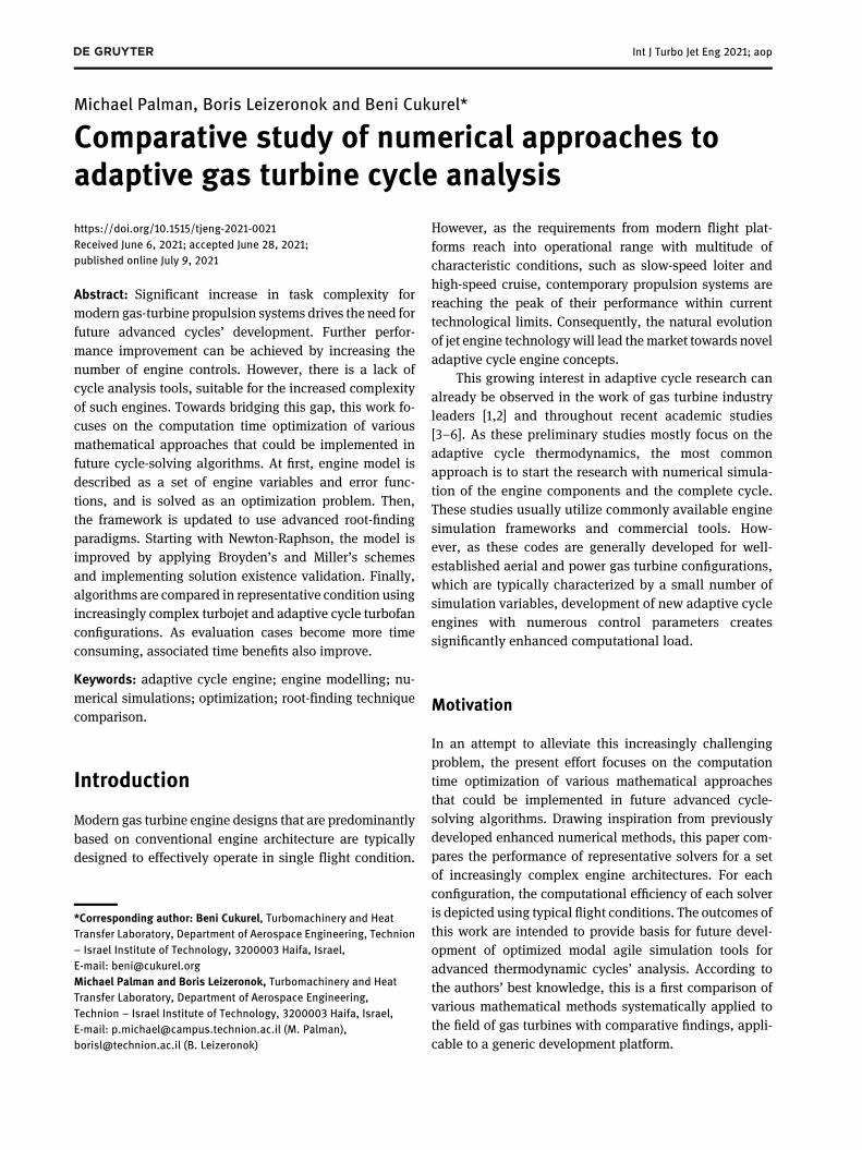
The proposed numerical approaches can be implementedinto optimized simulation tool, which can be validatedagainst commercial GasTurb13 software. Same single-spool turbojet engine is modeled in GasTurb13 and theresults of the commercial and in-house codes arecompared in Figures 12 and 13 in terms of operating line,thrust rating and fuel consumption respectively. Thefindings are in close agreement with 1.35% average devi-ation in operating line, 1.84% average deviation in thrustrating and 0.64% average deviation in fuel consumption.This deviation magnitude suggests that the algorithm is

Figure 11: Search for the upper (left) andlower (right) spline edge (M = 0.3,H = 5000 m, N = 0.38).

8 M. Palman et al.: Adaptive GT cycle analysis

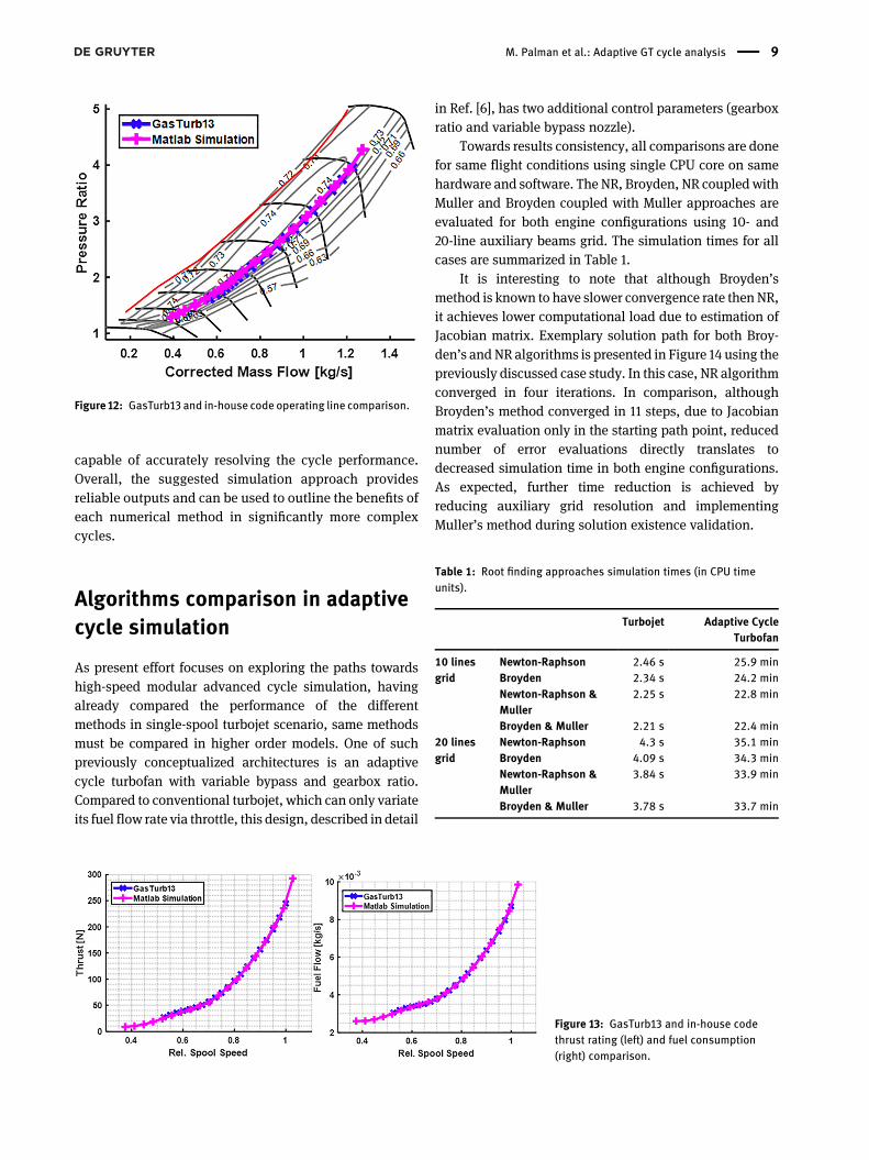
capable of accurately resolving the cycle performance.Overall, the suggested simulation approach providesreliable outputs and can be used to outline the benefits ofeach numerical method in significantly more complexcycles.

Algorithms comparison in adaptivecycle simulation

As present effort focuses on exploring the paths towardshigh-speed modular advanced cycle simulation, havingalready compared the performance of the differentmethods in single-spool turbojet scenario, same methodsmust be compared in higher order models. One of suchpreviously conceptualized architectures is an adaptivecycle turbofan with variable bypass and gearbox ratio.Compared to conventional turbojet, which can only variateits fuel flow rate via throttle, this design, described in detail

in Ref. [6], has two additional control parameters (gearboxratio and variable bypass nozzle).

Towards results consistency, all comparisons are donefor same flight conditions using single CPU core on samehardware and software. The NR, Broyden, NR coupled withMuller and Broyden coupled with Muller approaches areevaluated for both engine configurations using 10- and20-line auxiliary beams grid. The simulation times for allcases are summarized in Table 1.

It is interesting to note that although Broyden’smethod is known to have slower convergence rate then NR,it achieves lower computational load due to estimation ofJacobian matrix. Exemplary solution path for both Broy-den’s and NR algorithms is presented in Figure 14 using thepreviously discussed case study. In this case, NR algorithmconverged in four iterations. In comparison, althoughBroyden’s method converged in 11 steps, due to Jacobianmatrix evaluation only in the starting path point, reducednumber of error evaluations directly translates todecreased simulation time in both engine configurations.As expected, further time reduction is achieved byreducing auxiliary grid resolution and implementingMuller’s method during solution existence validation.

Figure 12: GasTurb13 and in-house code operating line comparison.

Figure 13: GasTurb13 and in-house codethrust rating (left) and fuel consumption(right) comparison.

Table : Root finding approaches simulation times (in CPU timeunits).

Turbojet Adaptive CycleTurbofan

linesgrid

Newton-Raphson . s . minBroyden . s . minNewton-Raphson &Muller

. s . min

Broyden & Muller . s . min linesgrid

Newton-Raphson . s . minBroyden . s . minNewton-Raphson &Muller

. s . min

Broyden & Muller . s . min

M. Palman et al.: Adaptive GT cycle analysis 9

To further highlight the difference between NR andBroyden methods, additional complexity can be added toengine architecture. For example, addition of recuperationto the cycle will impose another computational variableinto the algorithm. A simplified heat exchanger model canbe added according to Ref. [19].

Based on recuperator design condition, off-design ef-ficiency and pressure losses on the cold and the hot sidescan be evaluated. Efficiency is defined as

η = 1 − mmds

(1 − ηds), (17)

cold side pressure loss is evaluated from

Pin − Pout

Pin= (Pin − Pout

Pin)

ds

⎛⎝minPin⎞⎠2

T1.55out

T0.55in

⎛⎝minPin⎞⎠2

ds

T1.55out, ds

T0.55in, ds

, (18)

and hot side pressure loss is calculated via

Pin − Pout

Pin= (Pin − Pout

Pin)

ds

m2inTin

(m2inTin)

ds

. (19)

In recuperated engine cycle, combustor inlet temper-ature, which is the heat exchanger cold side outlet, is thenew simulation variable. Evaluated off-design efficiencyprovides hot side inlet temperature directly from heatexchanger efficiency definition

η = Tcold, out − Tcold, in

Thot, in − Tcold, in. (20)

After solving the combustion chamber and the turbinemodules, iterated recuperator efficiency is compared toinitial estimate. The difference between the two values isadditional simulation error. Thus, engine model formula-tion Should now be described by three variables and threeerror functions. In this case, the size of Jacobian matrixbecomes 3 × 3, significantly increasing the number of errorfunction evaluations.

This effect of adding heat exchanger module is eval-uated in both engine configurations. Design point effi-ciency of 80%with 3% pressure drop on both cold and hotside is assumed. The recuperated cycles are evaluated onlyusing 10-line auxiliary beams grid. Outcome of this inves-tigation is summarized in Table 2.

It can be observed that despite increased size of theJacobian matrix, due to pressure losses in the heatexchanger, the simulation times are close to non-recuperated engines. As pressure loss is directly propor-tional to engine flow rate, higher spool speeds imposehigher pressure loss. This phenomenon significantly re-duces the number of converged operating points, withunsuitable points filtered out by solution existence check.However, regardless of this effect, an increasing gap be-tween NR and Broyden’s methods can still be registered.

To highlight the usefulness of this simulationapproach, preliminary analysis of conceptual micro-turbojet to micro-turbofan conversion project can beconsidered. Using the same engine core, this would requireincreased power extraction from the turbine to support thefan stage. In this scenario, increased core inlet pressurewould not only allow higher turbine power, but would alsoresult in higher thermodynamic cycle efficiency. Althoughlarge-scale turbofan engines typically have booster stagesto achieve this effect, a different concept can be adopted inthis hypothetical micro gas turbine project, where smallspatial scales could potentially prevent booster installa-tion. Instead, hub loaded fan with higher hub pressureratio can perform as a booster stage. In this atypical case,the fan hub and tip regions will have separate fan maps,

Figure 14: Converged solution paths of Broyden’s and NR methods(M = 0.3, h = 5000 m, N = 0.38).

Table : Simulation time of recuperated engine configurations (inCPU time units).

Turbojet withHEX

Adaptive Cycle Turbofanwith HEX

Newton-Raphson . s . minBroyden . s . minNewton-Raphson &Muller

. s . min

Broyden & Muller . s min

10 M. Palman et al.: Adaptive GT cycle analysis

which need to be individually accounted by separate setsof β-coordinates, leading to increased simulation times.

To emphasize the differences between the solvers inthis case, they can be evaluated in realistic mission designspace. In this case, the enginemodel needs to be solved forranges of Mach numbers and altitudes. A realistic flightenvelope covers Mach range of 0–0.9 and altitude range of0–9 km and can be resolved with Mach number steps of 0.1and altitude steps of 1 km. Thus, the design space wouldresult in 81 distinct flight conditions. Knowing the repre-sentative solution time for each flight condition allowsevaluation of simulation time for the complete envelope.The results for each solver are summarized in Table 3.Clearly, in this case, simulation time is of tremendousimportance and optimized simulation methodology be-comes increasingly crucial tool.

It is important to note that although all cases werecompared using MATLAB towards simplicity and fasterimplementation, it is an interpretive programing language,which is relatively slow. For example, it is known to be upto 11 times slower than C++ programing language [20, 21].Thus, using compiled programming language and furtheroptimizing the code will lead to significantly reducedsimulation times akin to those, which are typical in variouscommercial cycle simulation codes. Regardless, the bene-fits of the presented methods will also scale accordingly.

Summary and conclusions

The present paper focuses on comparison of various nu-merical approaches in the framework of simulationdevelopment for increasingly complex engine models.Starting with outlining the numerical challenges of typicalmodular engine simulation tool, several paths are sug-gested to improve computation times for engine operatingpoint. At first, the engine model is solved as an optimiza-tion problem using surrogate and particle swarm ap-proaches. Although this formulation reduces simulation

time, the outcomes are insignificant on the grandscale.Moreover, parallelization attempts result in higher timeswhen compared to single core formulation.

In following, several suggestions are made to enhancethe classical solution procedure. NR algorithm is imple-mented to shorten the root finding time. To further reducecomputational load, a solution existence check method-ology is implemented and NR is replaced with significantlyfaster Broyden’s procedure. Additional improvement isdone by reducing auxiliary grid resolution and applyingMuller’s technique during computational domain identifi-cation phase. The combined effect of Muller’s and Broy-den’s techniques reduces the overall flight envelopesimulation time by 3.3, 7.3 and 12.3% when compared tocombination of Newton-Raphson and Muller’s methods,only Broyden’s method and only Newton-Raphsonmethod, respectively.

The impact of sequential code improvement is high-lighted in representative single-spool turbojet and adap-tive cycle turbofan configurations. As adaptive cycleengine has additional gear and bypass ratio control pa-rameters when compared to the turbojet architecture,which can only variate spool speed, the increased modelcomplexity results in significantly increased simulationtimes. The engine model is then further expanded toinclude recuperation. Although addition of heat exchangerimposes another degree of freedom, the pressure lossesreduce the number of converged engine operating points.Therefore, due to solution existence validation procedure,which filters un-convergable points prior to simulationstart, the computation time remains unchanged. Finally,micro-turbofan with hub loaded fan is considered and isused to highlight the code differences in realistic designspace.

According to the best knowledge, the present work isthe first quantitative comparison of individual solvers andtheir cumulative effect, particularly geared towardsadvanced gas turbine cycle simulations. It is the hope ofthe authors that the findings of this study would helpestablish the path towards future optimized simulationcodes, regardless of the selected implementationframework.

Author contributions: All the authors have acceptedresponsibility for the entire content of this submittedmanuscript and approved submission.Research funding: The present research effort was partiallysupported by the U.S. Office of Naval Research Global underaward number N62909-17-1-217; Peter Munk Research

Table : Adaptive cycle turbofan with booster flight envelopesimulation.

Adaptive Cycle Turbofanwith Booster

Flight EnvelopeSimulation

Newton-Raphson . h . dayBroyden . h . dayNewton-Raphson& Muller

. h . day

Broyden & Muller . h . day

M. Palman et al.: Adaptive GT cycle analysis 11

Institute under award number 110101; and the Bernard M.Gordon Center for Systems Engineering under awardnumber 1017930. Also, supported by Minerva ResearchCenter (Max Planck Society Contract No. AZ5746940764).Conflict of interest statement: The authors declare noconflicts of interest regarding this article.

References

1. WILLIAM K. Pratt and Whitney receives $437M for continuedadaptive engine development. Available from: https://www.sae.org/news/2018/09/pratt–whitney-receives-usd437m-for-continued-adaptive-engine-development.

2. Rolls-Royce. Rolls-Royce North American Technologies, Inc.Selected by U.S. Air Force to complete ADVENT researchdemonstrator Program. Available from: http://www.defense-aerospace.com/articles-view/release/3/109107/rolls_royce-selected-for-advent-demonstrator.html.

3. Kowalski M. Adaptive jet engines. J KONES Powertrain Transport2011;18.

4. Patel HR, Wilson DR. Parametric cycle analysis of adaptive. AIAAPropul Energy 2018. 2018 Joint Propulsion Conference, July 9-11,2018, Cincinnati, Ohio, US. https://doi.org/10.2514/6.2018-4521.

5. Visser MOWPJ, Kogenhop O. A generic approach for gas turbineadaptive modeling. J Eng Gas Turbines Power 2006;128:13–19.

6. Palman M, Leizeronok B, Cukurel B. Mission analysis andoperational optimizationof adaptive cyclemicroturbofan engine insurveillance and firefighting scenarios. J Eng Gas Turbines Power2019;141. https://doi.org/10.1115/1.4040734.

7. Kadosh K Cukurel B. Micro-turbojet to turbofan conversion viacontinuously variable transmission: thermodynamic performancestudy. ASME J Eng Gas Turbines Power 2017;139. https://doi.org/10.1115/1.4034262.

8. Lichtsinder M, Levy Y. Jet engine model for control and real-timesimulations. J Eng Gas Turbines Power 2006;128:745–53.

9. Powell MJD. The theory of radial basis function approximation in1990. In: Light WA, editor. Advances in numerical analysis,volume 2, wavelets, subdivision algorithms, and radial basisfunctions. Oxford: Clarendon Press; 1992:105–210 pp.

10. Regis RG, Shoemaker CA. A stochastic radial basis functionmethod for the global optimization of expensive functions. Inf JComput 2007;19:497–509.

11. Wang Y, Shoemaker CA. A general stochastic algorithmframework for minimizing expensive black box objectivefunctions based on surrogate models and sensitivity analysis.2014. arXiv:1410.6271v1. Available from: https://arxiv.org/pdf/1410.6271.

12. Gutmann H-M. A radial basis function method for globaloptimization. J Global Optim 2001;19:201–27.

13. Kennedy J, Eberhart R. Particle swarm optimization. In:Proceedings of the IEEE International Conference on NeuralNetworks. 1995:1942–5.

14. Mezura-Montes E, Coello CA. Constraint-handling in nature-inspirednumerical optimization: past, present and future. Swarmand Evolutionary Computation 2011;1:173–94.

15. Pedersen ME. Good parameters for particle swarm optimization.Luxembourg City, Luxembourg: Hvass Laboratories; 2010.

16. Ryaben’kii VS, v Tsynkov S. A theoretical introduction tonumerical analysis. BocaRaton, Florida, US: CRCPress; 2006:243p. ISBN 9781584886075.

17. Broyden CG. A class of methods for solving nonlinearsimultaneous equations math. Math Comput 1965;19:577–93.

18. Muller DE. A method for solving algebraic equations using anautomatic computer. MTAC; 1956. p. 208–15. https://doi.org/10.1090/s0025-5718-1956-0083822-0.

19. Walsh PP, Fletcher P. Gas turbine performance. Hoboken, NewJersey, US: Blackwell Publishing; 2004.

20. Gouy I. The computer language benchmarks game. Availablefrom: https://benchmarksgame-team.pages.debian.net/benchmarksgame.

21. AruobaSB, Fernansez-Villaverde J. A comparison of programminglanguages in macroeconomics. J Econ Dyn Control 2015;58:265–73.

12 M. Palman et al.: Adaptive GT cycle analysis