Michael M. Richter - University of Calgarypages.cpsc.ucalgary.ca/~mrichter/ML/ML 2010/Experience and...
74
Michael M. Richter University of Calgary 2010 Machine Learning Michael M. Richter Case Based Reasoning Email: [email protected]
Transcript of Michael M. Richter - University of Calgarypages.cpsc.ucalgary.ca/~mrichter/ML/ML 2010/Experience and...

Michael M. Richter University of Calgary
2010
Machine Learning
Michael M. Richter
Case Based Reasoning
Email: [email protected]

Michael M. Richter
Learning by Experience• Experiences are stored stories of
– successful solutions: Do it again!
– or failures: Avoid this!
• These stories are in a memory.
• We have two problems to use them:
– The situation in the experience is not exactly the same as the
actual solution
– How to find the most useful experience?
• For the first problem we observe that the experience is
not totally different from the actual situation; it is similar or
analogous.
• Experiences are also called cases.
University of Calgary
2010

Michael M. Richter
Case Based Reasoning
• Case Based Reasoning makes systematic use of these
ideas.
• Central is the concept of similarity: It determines when an
old experience is possibly useful for solving a new
problem.
• The success depends on:
– The set of available cases (the case base)
– The quality of the similarity measure.
• This approach has been generalized to situation where
no experiences are available by establishing a similarity
between the problem and the solution directly.
University of Calgary
2010

Michael M. Richter
University of Calgary
2009
-
Description of an Experience (1)
• We deal with a particular diagnostic situation
• The story records several features and their specific values
occurred in that situation.
Feature Value
Problem (Symptoms)
• Problem: Front light doesn’t work
• Car: VW Golf IV, 1.6 l
• Year: 1998
• Battery voltage: 13,6 V
• State of lights: OK
• State of light switch: OK
Solution
• Diagnosis: Front light fuse defect
• Repair: Replace front light fuse
C
A
S
E
1

Michael M. RichterUniversity of Calgary 20
2010-
Description of an Experience (2)
• Each case
describes one
particular situation
• All cases are
independent of
each other
Problem (Symptoms)
• Problem: Front light doesn’t work
• Car: VW Golf III, 1.6 l
• Year: 1996
• Battery voltage: 13,6 V
• State of lights: OK
• State of light switch: OK
Solution
• Diagnosis: Front light fuse defect
• Repair: Replace front light fuse
C
A
S
E
1
Problem (Symptoms)
• Problem: Front light doesn’t work
• Car: Audi A4
• Year: 1997
• Battery voltage: 12,9 V
• State of lights: surface damaged
• State of light switch: OK
Solution
• Diagnosis: Bulb defect
• l: Replace front light
C
A
S
E
2
Now we have two
experiences

Michael M. Richter
University of Calgary
2009
-
Finding an Experience (1)
• Now: A new problem has to be solved
• We make several observations in the current situation
• Observations define a new problem
• Not all feature values have to be known
Note: The new problem is a “case” without solution part
FeatureValue
Problem (Symptom):
• Problem: Break light doesn’t work
• Car: Audi 80
• Year: 1989
• Battery voltage: 12.6 V
• State of light: OK

Michael M. Richter
University of Calgary
2010
-
Finding an Experience (2)
• When are two cases similar?
• How to rank the cases according to their similarity?
Similarity is crucial!
• We can assess similarity based on the similarity of each feature
• Similarity of each feature depends on the feature value.
• BUT: Importance of different features may be different
New Problem
C
A
S
E
x
Similar?
Compare the New Problem with Each Case
What is the most useful experience?

Michael M. RichterUniversity of Calgary 2010
-
Finding an Experience (3)
• Assignment of similarities for features values.
• Express degree of similarity by a real number between 0 and 1
• Examples:
– Feature: Problem
– Feature: Battery voltage (similarity depends on the difference)
• Different features have different importance (weights)!
– High importance: Problem, Battery voltage, State of light, ...
– Low importance: Car, Year, ...
Not similar Very similar
Front light doesn’t work Break light doesn’t work
Front light doesn’t work Engine doesn’t start
0.8
0.4
12.6 V 13.6 V
12.6 V 6.7 V
0.9
0.1

Michael M. Richter
University of Calgary
2010
-
Finding an Experience (4)
• Similarity computation by weighted average similarity(new,case 1) = 1/20 * [ 6*0.8 + 1*0.4 + 1*0.6 + 6*0.9 + 6* 1.0 ] = 0.86
Problem (Symptom)
• Problem: Break light doesn’t work
• Car: Audi 80
• Year: 1989
• Battery voltage: 12.6 V
• State of lights: OK
Experience 1 (Symptoms)
• Problem: Front light doesn’t work
• Car: VW Golf III, 1.6 l
• Year: 1996
• Battery voltage: 13.6 V
• State of lights: OK
• State of light switch: OK
Solution
• Diagnosis: Front light fuse defect
• Repair: Replace front light fuse
0.8
0.4
0.6
0.9
1.0
Very important feature: weight = 6
Less important feature: weight = 1

Michael M. Richter
University of Calgary
2010
-
Finding an Experience (5)
• Similarity computation by weighted average similarity(new,case 2) = 1/20 * [ 6*0.8 + 1*0.8 + 1*0.4 + 6*0.95 + 6*0 ] = 0.585
Case 1 is more similar: due to feature “State of lights”
Problem (Symptom)
• Problem: Break light doesn’t work
• Car: Audi 80
• Year: 1989
• Battery voltage: 12.6 V
• State of lights: OK
Experience 2 (Symptoms)
• Problem: Front light doesn’t work
• Car: Audi A4
• Year: 1997
• Battery voltage: 12.9 V
• State of lights: surface damaged
• State of light switch: OK
Solution
• Diagnosis: Front light fuse defect
• Repair: Replace front light fuse
0.8
0.8
0.4
0.95
0
Very important feature: weight = 6
Less important feature: weight = 1

Michael M. Richter University of Calgary
2010
Using an Experience
• New Solution:
• Diagnosis: Break light fuse defect
• Repair: Replace break light fuse
Problem (Symptom):
• Problem: Break light doesn’t work
• Car: Audi 80
• Year: 1989
• Battery voltage: 12,6 V
• State of light: OK
Adapt Solution:
How do differences in the
problems affect the solution?
Problem (Symptoms):
• Problem: Front light doesn’t work
• ...
Solution:
• Diagnosis: Front light fuse defect
• Repair: Replace front light fuse
C
A
S
E
1
Observation: case 1 is not the same as the new problem!!

Michael M. Richter
University of Calgary
2010
-
An Application Scenario:
Call Centre• Technical Diagnosis of Car Faults:
– symptoms are observed (e.g., engine doesn’t start) and
values are measured (e.g., battery voltage = 6.3V)
– goal: Find the cause for the failure (e.g., battery empty) and
a repair strategy (e.g., charge battery)
• Case-Based Diagnosis:
– a case describes a diagnostic situation and contains:
• description of the symptoms
• description of the failure and the cause
• description of a repair strategy
– store a collection of cases in a case base
– find case similar to current problem and reuse repair strategy

Michael M. Richter
University of Calgary
2010
-
Difference to Other Methods
• Learning in CBR does not generate an explicit generalization
• Learning = Storage of specific experiences
• Problem solving: Using specific experiences by analogy
• Contrast:
• Generalization = Compilation of experiences
• Learning by similarity = Interpretation of experiences
ex1, ex2, .....exn ex1, ex2, .....exn
compilation interpretation
Michael M. Richter
University of Calgary
2010
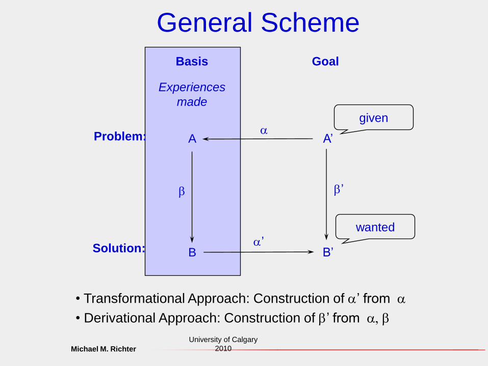
General Scheme
A
B
A’
B’a’
a
b b’
Basis Goal
Experiences
made
Problem:
Solution:
given
wanted
• Transformational Approach: Construction of a’ from a
• Derivational Approach: Construction of b’ from a, b

Michael M. Richter
University of Calgary
2010
-
Transformational Approach (1)
• Transform the solution of a similar problem
New Solution
New ProblemSimilarity
Solution transformation
Solution
Problema
a’
b
Eperiences made

Michael M. Richter University of Calgary 2010
-
Transformational Approach (2)• Previous experiences are stored:
Problem + Solution
• General approach:
– Search in the experience data base for experiences with similar
problem descriptions
– Find the solution belonging to the old problem description
– (incremental) transformation of the old solution until it satisfies the
demands and constraints of the new problem sufficiently well.
– Validation of the found solution
– If the transformation had no success or the found solution was
incorrect: Search for other experiences

Michael M. Richter
University of Calgary
2010
-
Derivational Approach (1)
• Transform the inference leading to the solution of a
similar problem:
New
Problem
Solution of the
new problem
solved
problem2
Solution of the
old problem2
partial mapping
Solution of the
old problem1
Solved
problem1
Recall
the inference
influ
ences
Michael M. RichterUniversity of Calgary 2010
-
Derivational Approach (2)
• Previous experiences are stored:
Problem + Solution + Inference (solution path)
• General approach:
– Search in an experience data base for experiences with similar
problem descriptions
– Isolate commonalities between the actual problem and the
experiences.
– Determine those parts of the solution paths that can be
transformed.
– Recall the found partial solution paths in the context of the actual
problem.
Michael M. Richter
University of Calgary
2010
-
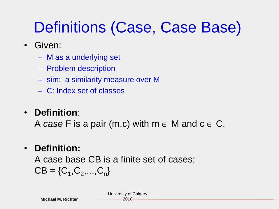
Definitions (Case, Case Base)• Given:
– M as a underlying set
– Problem description
– sim: a similarity measure over M
– C: Index set of classes
• Definition:
A case F is a pair (m,c) with m M and c C.
• Definition:
A case base CB is a finite set of cases;
CB = {C1,C2,...,Cn}
Michael M. Richter
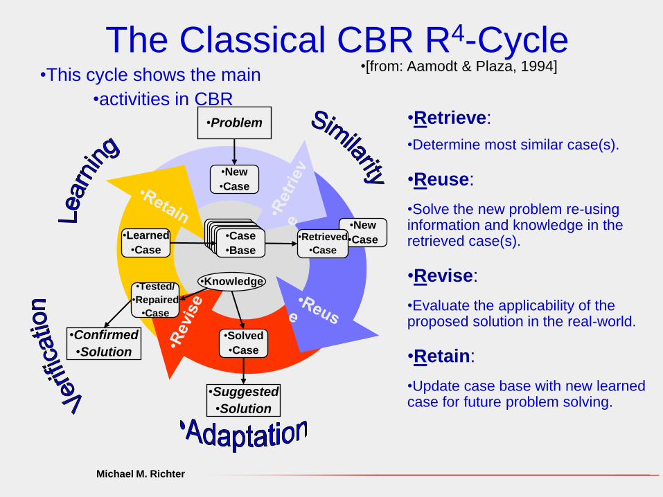
The Classical CBR R4-Cycle•[from: Aamodt & Plaza, 1994]
•Retrieve:
•Determine most similar case(s).
•Reuse:
•Solve the new problem re-using information and knowledge in the retrieved case(s).
•Revise:
•Evaluate the applicability of the proposed solution in the real-world.
•Retain:
•Update case base with new learned case for future problem solving.
•Case
•Base
•Knowledge
•New
•Case
•New
•Case•Retrieved
•Case
•Solved
•Case
•Learned
•Case
•Tested/
•Repaired
•Case
•Suggested
•Solution
•Problem
•Confirmed
•Solution
•This cycle shows the main
•activities in CBR
Michael M. Richter
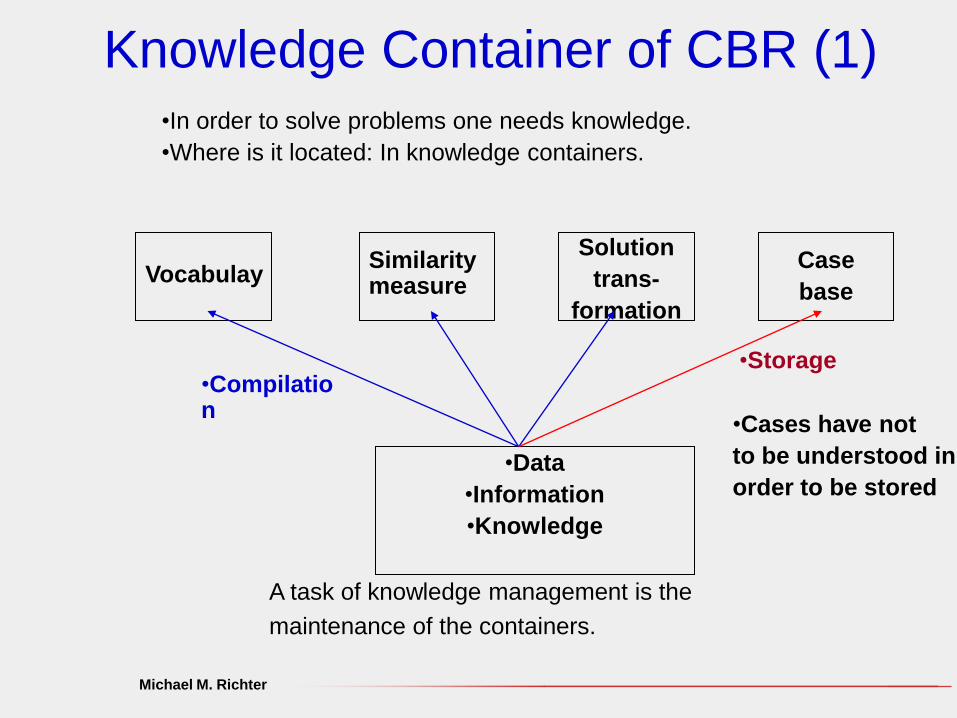
Knowledge Container of CBR (1)
Solution
trans-
formation
Case
baseVocabulay
Similaritymeasure
•Data
•Information
•Knowledge
•Storage•Compilation
•Cases have not
to be understood in
order to be stored
•In order to solve problems one needs knowledge.
•Where is it located: In knowledge containers.
A task of knowledge management is the
maintenance of the containers.

Michael M. Richter
The Knowledge Containers (2)
University of Calgary 2010
-

Michael M. Richter University of Calgary 2010
-
Similarity Measures
• Idea: Numerical modeling of similarity (more or less similar)
• Along with ordinal information there is also a quantitative
statement about the degree of similarity:
• Definition: A similarity measure on a set M is a real function
sim: M2 [0,1]. The following properties can hold:
– " x M: sim(x,x) = 1 (Reflexivity)
A similarity measure is symmetrical ) :
– " x,y M: sim(x,y) = sim(y,x) (Symmetry)
• Induced similarity relation:
– sim(x,y) > sim(x,z) “x is more similar to y than to z”
0 1
sim(x,yi)
y1y2y3y4
Michael M. Richter University of Calgary 2010
-
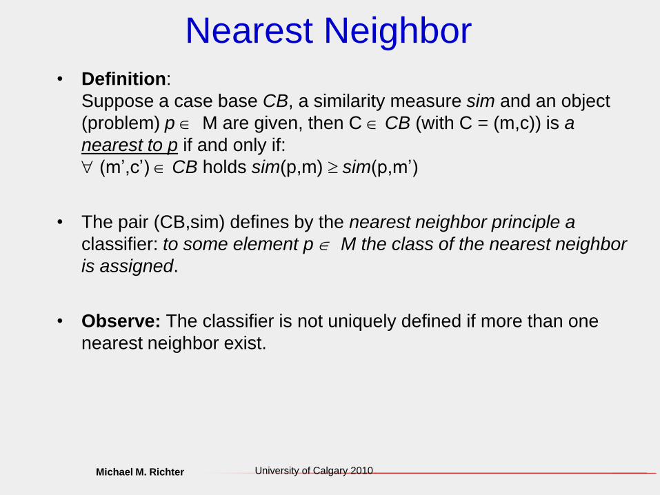
Nearest Neighbor• Definition:
Suppose a case base CB, a similarity measure sim and an object
(problem) p M are given, then C CB (with C = (m,c)) is a
nearest to p if and only if:
" (m’,c’) CB holds sim(p,m) sim(p,m’)
• The pair (CB,sim) defines by the nearest neighbor principle a
classifier: to some element p M the class of the nearest neighbor
is assigned.
• Observe: The classifier is not uniquely defined if more than one
nearest neighbor exist.

Michael M. Richter University of Calgary 2010
-
Distance Functions / Measures• Instead of using similarity functions often one takes distance functions,
the dual notion.
• Definition: A distance measure on a set M is a real valued function d: M2 IR+.
• The following properties can hold:
– " x M d(x,x) = 0 (Reflexivity)
A distance measure is symmetrical ) :
– " x, y M d(x,y) = d(y,x) (Symmetry)
A distance measure is a metric ) :
– " x, y M d(x,y) = 0 x = y
– " x, y, z M d(x,y) + d(y,z) d(x,z) (Triangle Inequality)
• Induced similarity relation:
– d(x,y) < d(x,z) “x is more similar (less distant) to y than to z”
Michael M. Richter University of Calgary 2010
-
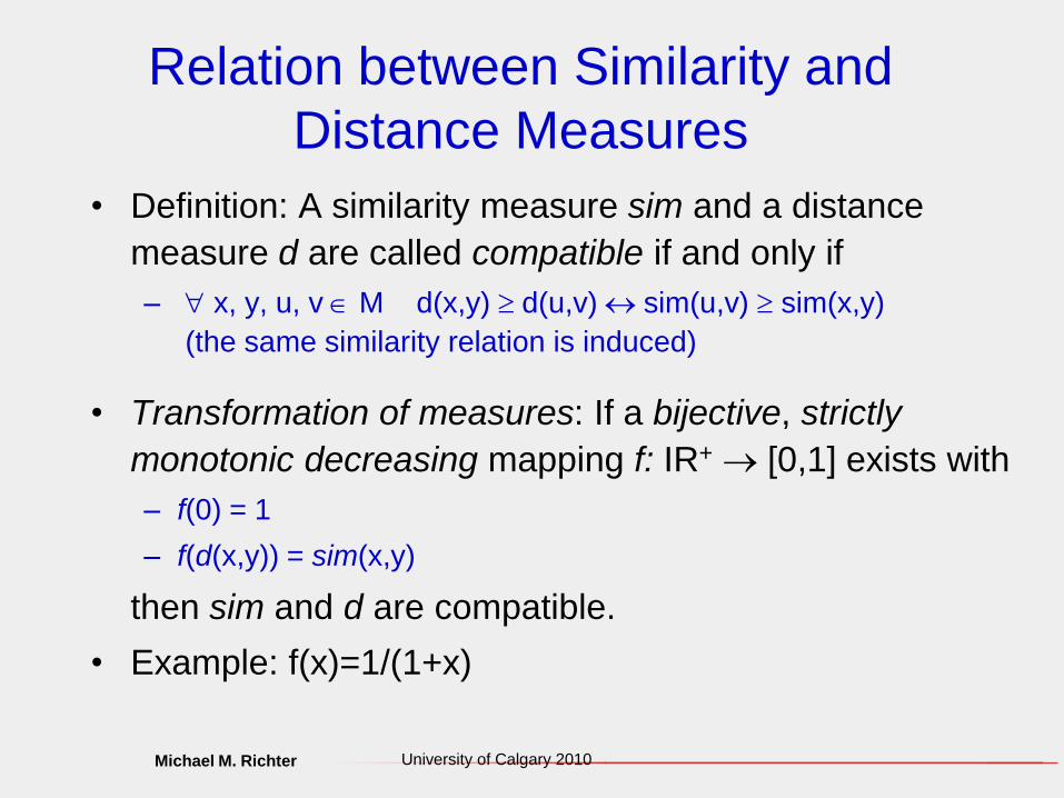
Relation between Similarity and
Distance Measures
• Definition: A similarity measure sim and a distance
measure d are called compatible if and only if
– " x, y, u, v M d(x,y) d(u,v) sim(u,v) sim(x,y)
(the same similarity relation is induced)
• Transformation of measures: If a bijective, strictly
monotonic decreasing mapping f: IR+ [0,1] exists with
– f(0) = 1
– f(d(x,y)) = sim(x,y)
then sim and d are compatible.
• Example: f(x)=1/(1+x)

Michael M. Richter University of Calgary 2010
-
Example 1: Hamming Disance and
Simple Matching Coefficient
• Regarding similarity between two objects x and y:
x = (x1,...,xn) xi {0,1}
y = (y1,...,yn) yi {0,1}
• Distance Measure:
• Properties:
– H(x,y) [0,n] n is the maximum distance
– H(x,y) is the number of distinguishing attribute values
– H is a distance measure:
• H(x,x) = 0
• H(x,y) = H(y,x)
– H( (x1,...,xn), (y1,....,yn) ) = H( (1-x1,...,1-xn), (1-y1,....,1-yn) )
H x y n x y x yi ii
n
i ii
n
( , ) ( ) ( )
1 1
1 1

Michael M. Richter University of Calgary 2010
-
Examples 2 : Real-Valued Attributes
• Real-valued attributes xi , yi IR for all i
• Generalization of the Hamming Distance to the
City-Block-Metric:
• Alternative metrics
Euclidean Distance:
Weighted Euclidean Distance:
d x y x yi i
i
n
( , ) | |
1
d x y x yi i
i
n
( , ) ( )
2
1
d x y x yi i i
i
n
( , ) ( )
a 2
1

Michael M. Richter
Weights
• The weighted Euclidean measure takes care of the fact that
not all attributes are of the same importance.
• Higher weight means that the attribute has more influence on
the measure and on the chance to be selected as nearest
neighbor.
• Weights are a general means to reflect importance and can
be applied in a wide range of measures.
• Often, the choice of good weights is a major and difficult task
that can require additional learning methods.
University of Calgary
2010

Michael M. RichterUniversity of Calgary 2010
-
A General Similarity
Measure
• Given two problem descriptions C1, C2
• p attributes y1, ..., yp used for the representation
p
1j
jj (C1,C2)simSIM(C1,C2) ω
simj : similarity for attribute j (local measure)
wj : describes the relevance of attribute j for the problem

Michael M. Richter University of Calgary 2010
-
Classifiers• (CB,sim) is a classifier description
• The description is distributed over CB and sim; a
change of CB or sim can lead to a different classifier
• Two extreme cases:
a) The whole classification information is in the case base:
• CB = { (p, class(p)) | p M }
• sim(x,y) = 1 if x=y
sim(x,y) < 1 otherwise
b) The whole classification information is in the similarity measure:
• CB = “One case per class”
• sim(x,y) = 1 if class(x) = class(y)
sim(x,y) < 1 otherwisemeasure
knows the
classifier
trivial measure

Michael M. Richter
No Experiences
• Often, no experiences are available. This is e.g. the case
in e-commerce where no specific (problem, demand)
solutions are recorded.
• Instead one records directly the similarity between
problems and solutions.
• An example in e-commerce is the similarity between a
demand and an available product.
• The analog of a case base is now a product base and the
nearest neighbor to a demand is a product that satisfies
the customer demand in an optimal way.
• In general, the products are again called cases.
University of Calgary
2010

Michael M. Richter
Example : Selling Cars
• The problem is a customer demand:
– Description D of a demanded car
• Case base:
– Descriptions of the available cars C
• The customer is offered a car C where
sim(D, C) is maximal
• The does not refer to previous sales.
• The CBR techniques remain the same.
• However, previous sales may be used for improving the
similarity measure.
University of Calgary
2010

Michael M. Richter
How to Determine the Weights? (1)
• Basic idea: Weights reflect importance
• Importance for what? For finding a good solution.
• That means, if we consider just one attribute A, it is more
important than an attribute B if the solution found by using
A is better than using B.
• Better can mean different things, e.g.
– The probability for finding the correct solution is higher
– The expected costs for false solutions are lower
– Etc
• These aspects should be reflected in the weights
University of Calgary 2010
Michael M. Richter
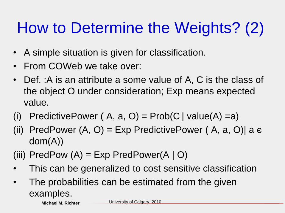
How to Determine the Weights? (2)
• A simple situation is given for classification.
• From COWeb we take over:
• Def. :A is an attribute a some value of A, C is the class of
the object O under consideration; Exp means expected
value.
(i) PredictivePower ( A, a, O) = Prob(C | value(A) =a)
(ii) PredPower (A, O) = Exp PredictivePower ( A, a, O)| a є
dom(A))
(iii) PredPow (A) = Exp PredPower(A | O)
• This can be generalized to cost sensitive classification
• The probabilities can be estimated from the given
examples.University of Calgary 2010

Michael M. Richter University of Calgary 2010
-
Learning of Attribute Weights• Goal: Improved similarity measure by weight
adaptation
• There are different ways to model weights:
– global weights:
– local (class specific) weights:
wij: Relevance matrix
– case specific weights:
• Adaptation of weights: Change the relevance of
features for the solution.
sim q c w sim q ci i i i
i
n
( , ) ( , )
1
sim q c w sim q ci class c i i i
i
n
( , ) ( , ), ( )
1
sim q c w sim q ci c i i i
i
n
( , ) ( , ),
1

Michael M. Richter
Local Similarity Measures
for Integer/Real
• Similarity often based on difference:– linearly scaled value ranges: simA(x,y) = f(x-y)
– exponentially scaled value ranges: simA(x,y) = f(log(x)-log(y))
• Generally, for f we claim:– f: IR [0..1] or Z [0..1]
– f(0) = 1 (Reflexivity)
– f(x): monotonously decreasing for x>0 and monotonously increasing for x<0
– Examples:
•1
•f
•symmetric
•1
•f
•asymmetric
•x: query; y: case
•query is minimum demand
•asymmetric
•x: query; y: case
•query is maximum demand
•1
•f
Michael M. Richter
Property:
Continuous or Sudden Decrease
• Depending on the distance between two values,
distinguish between decrease
– at a point ( Example a))
– in an interval ( Example b))
• Example:
a) decrease of the whole similarity at the distance X
b) decrease in the interval [xmin;xmax]•sim
•d•X •x•max
•min•x
•a)
•b)

Michael M. Richter
Local Similarities for Taxonomies (1)
• Assumption: considered objects can be ordered in a Taxonomy or set
of notions (tree or graph structure)
• Example:
• The ELSA 2000 is more similar to the Stealth 3D than to one of the S3 Trio adapters or MGA adapters.
Graphics Card
S3 Graphics Card MGA Graphics Card
ELSA 2000 Stealth 3D200 Miro Video
Matrox Mill. 220 Matrox Mystique
220
VGA V64
S3 Virge Card S3 Trio Card

Michael M. Richter
Local Similarities for Taxonomies (2)
• Definition of similarity for leaf nodes:
– assignment of a similarity value to each inner node
– similarity values for successor nodes become larger
– similarity between two leaf nodes is computed by the
similarity value at the deepest common predecessor
• Example:
sim (ELSA 2000, Stealth 3D) = 0,7
sim (ELSA 2000, VGA V64) = 0,5
sim (ELSA 2000, Matrox Mill.) = 0,2
Graphics Card
S3 Graphics Card MGA Graphics Card
ELSA 2000 Stealth 3D200 Miro Video
Matrox Mill. 220 Matrox Mystique
220
VGA V64
S3 Virge Card S3 Trio Card•0.7 •0.9
•0.5 •0.8
•0.2

Michael M. Richter
University of Calgary 2010
-
Learning of Weights with/without Feedback
• Many learning methods for both variants are known.
• Learning of Retrieval / Reuse without Feedback
– Make use of the distribution of cases in the case base for
determining the relevance of features
• Learning with Feedback
– Correct or false case selection / classification result leads to
correction of weights
+
+
A1
+
+
-
-
-
-
A2
A1 is more important than A2

Michael M. Richter University of Calgary 2010
-
Learning of Weights without Feedback• Detemination of class specific weights:
– Binary coding of the attributes by
• Discretization of integer and real valued attributes
• Transformation of symbolic attributes to n binary attributes
– Suppose
• wik is the weight for attribute i for class k
• class(c) is the class (solution) in case c
• ci the attribute i of case c
– Set: wik = Prob( class(c)=k | ci)
Conditional probability for a class k of c under the condition
of attribute ci.
– Estimate of the probabilities is done using “samples” of the
case base.

Michael M. Richter University of Calgary 2010
-
Learning of Weights with Feedback
• Correct or false classification leads to a correction of the
weights:
wik := wik + Dwik
• Different variants for determining the weight changes:
• Approach of Salzberg (1991) for binary attributes:
– Feedback = positive (correct classification):
• Weight of coincident attributes is increased
• Weight of differing attributes is decreased
– Feedback = negative (false classification):
• Weight of coincident attributes is decreased
• Weight of differing attributes is increased
– Here: Dwik is constant.

Michael M. Richter
University of Calgary 2010
-
Feedback Method: Gradient Descent
• We consider the classification error
• Experimentally to determine: e.g. leave-one-out test
• Goal: Optimizing the values of the weights s.t., e.g.
classification quality becomes optimal.
• Change of weights
in direction of steepest descent.
• Compare: Backpropagation
E (classification error)
w
best weight

Michael M. Richter University of Calgary 2010
-
Algorithm for Gradient Descent
1. Initialize the weight vector w and die learning rate l
2. Compute the error E(w) for the weight vector w
3. While not stop criterion Do
a) Learning step:
b) Compute:
c) If Then Else
" a w w Ea a
wa
:
l
E w( )
E w E w( ) ( )< w w: ll
2

Michael M. Richter University of Calgary 2010
-
Learning Rate
• Choice of the learning rate l

Michael M. Richter University of Calgary 2010
-
Further Parameters of the Algorithm
• Choice of the the stop-criterion:
– Fixed number of steps
– Minimal change of the error function
– Minimal change of the weights
– Minimal change of the learning rate

Michael M. Richter
University of Calgary 2010
-
Retrieval Methods
• There are many retrieval methods
• Trivial but too slow: Sequential Retrieval
• Important: k-dimensional binary search tree (Bentley,
1975).
• Idea: Decompose data (i.e. case base) iteratively in
smaller parts
• Use a tree structure
• Retrieval:
– Searching in the tree top-down with backtracking

Michael M. Richter
University of Calgary 2010
-
Example: kd-Tree
10 20 30 40 50 60 70
10
20
30
40
50
A1
A2
A
B
C
D
E
FG
H
I
C(20, 40)
E(35, 35)
H(70, 35)
I(65, 10)
F(50, 50)
G(60, 45)
A1
A(10, 10) B(15, 30) D(30, 20)
A2A2
A1
>35
>35>30
>15
<35
<30 <35
<15
CB={A,B,C,D,E,F,G,H,I}

Michael M. Richter
University of Calgary 2010
-
Definition: kd-Tree• Given:
– k ordered domains T1,...,Tk of the attributes A1,...,Ak,
– a base CB T1x...xTk. and
– some parameter b (bucket size).
A kd-tree T(CB) for the base CB is a binary tree
recursively defined as:
– if |CB| b: T(CB) is a leave node (called bucket) which is
labelled with CB
– if |CB| > b: T(CB) then T(CB) is a tree with the properties:
• the root is labelled with an attribute Ai and a value viTi
• the root has two kd-treesT (CB) and T>(CB>) as successors
• where CB := {(x1,...,xk) CB | xi vi} and
CB> := {(x1,...,xk) CB | xi > vi}

Michael M. Richter
University of Calgary 2010
-
Properties of a kd-Tree
• Ein kd-tree partitions a base:
– the root represents the whole base
– a leave node (bucket) represents a subset of the base which is
not further partitioned
– at all inner nodes the base is further partitioned s.t. base is
divided according to the value of some attribute.

Michael M. Richter University of Calgary 2010
-
Retrieval with kd-Trees
?
BOB test:Ball-overlap-Boands
1. Search the tree top-down to a leave
2. compute similarity to objects found
3. Determine termination by BWB-test
4. Determine additional candidates usinga BOB-test
5. If overlapping buckets existthen search in alternative branches(back to step 2)
6. Stop if no overlapping buckets
Idea for an algorithm:
overlap
?Most similarobject in the bucket
BWB testBall-within-Boands
Most similarobject in the
bucket

Michael M. Richter University of Calgary 2010
-
BOB-Test: Ball-Overlap-Bounds
?
m-most similar object in scq
overlap
boundaries of
the actual node
n-dimensional
hyper ball
A1
A2
Are there more similar objects then the m-most similar object
found in the neighbor subtree ?

Michael M. Richter University of Calgary 2010
-
BWB-Test: Ball-Within-Bounds
Is there no object in the neighboring subtree
that is more similar than the m-most-object?
? m-most-similar object in scq
A1
A2
boundaries of
the actual node
n-dimensional
hyper balll

Michael M. Richter University of Calgary 2010
-
Case Based Learning• Given: A sequence of training cases C1, C2 ,..., Ck
• Ddfinition:
• Case based learning determines, starting with an
empty case base CB0 and an initial measure sim0 a
sequence of tupels:
(CB1,sim1),(CB2,sim2),...,(CBk,simk) with CBi
{C1,...,Ci}
With each occurence of a training case can happen:
– the case base is changed (e.g. by including the case)
– the measure is changed
– both are changed

Michael M. Richter
University of Calgary 2010
-
Information in Similarity Measures
• Goal: Mesure the knowledge contained in similarity
measures:
• Def: The measure sim1 of a case based system
S1=(CB,sim1) is relative to CB better informed than the
measure sim2 of the system S2=(CB,sim2), if S1 classifies
more cases correctly than S2.
• Def: A case base CB of a case based system (CB,sim) is
called minimal if there is no case base CB’ CB s.t.
(CB’,sim) classifies at least so many cases correctly than
(CB,sim) does.
Michael M. Richter University of Calgary 2010
-
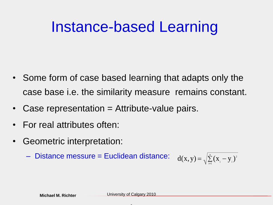
Instance-based Learning
• Some form of case based learning that adapts only the
case base i.e. the similarity measure remains constant.
• Case representation = Attribute-value pairs.
• For real attributes often:
• Geometric interpretation:
– Distance messure = Euclidean distance:
n
1i
2
ii)yx()y,x(d

Michael M. Richter
University of Calgary 2010
-
Three Incremental Learning Algorithms
IB1, IB2, IB3• Given:
– Similarity measure: Euclidean distance
– Sequence of training examples C1,C2,...,Cn
• Wanted:
– case base CB = CBn
• Approach:
– Determine a sequence of case bases CB1,...,CBn
• ThreeVariants:
– IB1: Takes all cases into the case base
– IB2: Takes cases only if the actual case base performs a
misclassification
– IB3: Takes cases only if the actual case base performs a
misclassification and removes in addition „bad“ cases.

Michael M. Richter University of Calgary 2010
-
IB1Let T = (F1,...,Fn) be the given sequence of training
examples
algorithm:
CB = {}
FOR i=1 to n DO
CB := CB {Fi}
Problem:
– case base grows fast.
– If IB1 would be used in the Retain-Phase of the CBR-Cycle then
tshe case base would grow each time a problem is solved

Michael M. Richter University of Calgary 2010
-
IB2Let T = (F1,...,Fn) be the given sequence of training
examples
algorithm:
CB={}
FOR i=1 to n DO
Set Ci = (p,c) (* p = problem; c = class*)
Choose from CB a case C’=(p’,c’) which is a nearest
neighbor to Ci .
IF c c’ THEN (* Failure *)
CB := CB {Fi}

Michael M. Richter University of Calgary 2010
-
Properties of IB2• IB2 depends on presentations sequence!
– Although a training case is correcty classified in the training
phase and is therefore not taken into the case base it may
very well happen that this case is misclassified in the final
case base.
• IB2 stores much less cases.
• In experiments: IB2 has a classification performance
almost as good as IB1.
1+
2-
3+4-
Is not stored
Michael M. Richter University of Calgary 2010
-
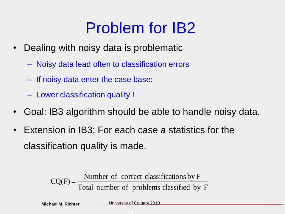
Problem for IB2• Dealing with noisy data is problematic
– Noisy data lead often to classification errors
– If noisy data enter the case base:
– Lower classification quality !
• Goal: IB3 algorithm should be able to handle noisy data.
• Extension in IB3: For each case a statistics for the
classification quality is made.
Fby classified problems ofnumber Total
Fby tionsclassificacorrect ofNumber )F(CQ

Michael M. Richter University of Calgary 2010
-
IB3 (1)Let T = (F1,...,Fn) be the given sequence of training examples
Algorithm:
CB={}
FOR i=1 to n DO
Let Fi = (p,c) (* p = problem; c = class*)
CBacc := { F CB | acceptable(F) }
IF CBacc {}
THEN
choose from CBacc a case F’=(p’,c’) which is a
nearest neighbor to Fi.
ELSE
choose randomly between 1 and |CB|
choose from CB a case F’=(p’,c’) which has the
j-largest similarity to Fi hat.
IF c c’ THEN CB := CB {Fi}

Michael M. Richter University of Calgary 2010
IB3(2)Continuation of the algorithm (still in the outer loop):
FOR ALL F*=(p*,c*) from CB with sim(p,p*) sim(p,p’) DO
update the statistics CQ(F) depending on c and c*:
- for correct classification (c=c*) increase denominator and numerator of
CQ(F);
- for false classification (cc*) increase denominator of KG(F).
IF F* is significantly bad THEN
CB := CB \ {F*}
CB
CBacc
acceptable?significantly bad?

Michael M. Richter
University of Calgary 2010
-
Criteria: Acceptable and Significantly
Bad
• Different statistical measures for the classification quality
are possible.
• A simple variant:
acceptable(F) iff CQ(F) > q1
F is significantly bad iff CQ(F) < q2
q1 and q2 are parameters with with which the algorithm
can be controlled.
Michael M. Richter University of Calgary 2010
-
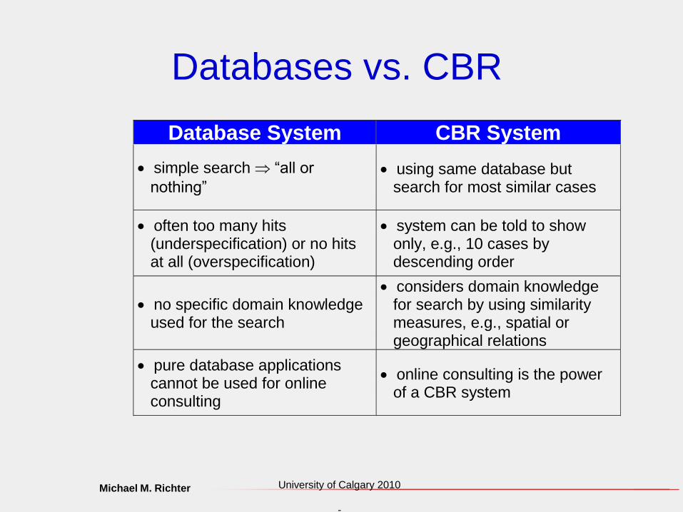
Databases vs. CBR
Database System CBR System
simple search “all or
nothing” using same database but
search for most similar cases
often too many hits(underspecification) or no hitsat all (overspecification)
system can be told to showonly, e.g., 10 cases bydescending order
no specific domain knowledgeused for the search
considers domain knowledgefor search by using similaritymeasures, e.g., spatial orgeographical relations
pure database applicationscannot be used for onlineconsulting
online consulting is the powerof a CBR system

Michael M. Richter University of Calgary 2010
-
Example: SIMATIC Knowledge
Manager• Customers use a www site to describe the problem in
terms of
– a textual query
– some information of the domain and the devices involved.
• By similarity based retrieval the most useful document is
presented to the customer.
• There are three types of documents:
– FAQ’s: Contain well established knowledge
– User information notes: Are less reliably
– Informal notes: Draft notes which give informal hints and may be
unreliable.

Michael M. RichterUniversity of Calgary 2010
-
SIMATIC KM (FAQ 241)Title: Order numbers of CPUs
with which communication is
possible.
Question: Which order
numbers must the S7-CPUs
have to be able to run basic
communications with SFCs?
Answer: In order to
participate in
communications via SFCs
without a configured
connection table, the
module needs the correct
order number. The following
table illustrates which order
number your CPU must
have to be able to
participate in these S7
homogeneous
communications.

Michael M. Richter University of Calgary 2010
-
SIMATIC Knowledge Manager
www.ad.siemens.de
Case Server
Structure
Information about the
Structure of the
SIMATIC Information
System
Order No.
Relation
order numbers
-productnames
Dictionary
InformationEntities
Similarities
Similarity model
Documents in the Customer SupportInformation System

Michael M. Richter
Positioning the CBR Method
•Closed Knowledge Model •Open Database
•Expert Systems
•CBR Systems
•Databases
•Increasing
•Knowledge Centralization
•Increasing
•Example Orientation
•Knowledge,•Models
•Data,•Examples
•Case Base
•Knowledge Model
•Similar•Case
•New•Case
•Adapted•Solution
•*
•*•
•Verified•Solution
•*•
•Stored•Solution
•RETRIEVE
•REUSE•REVISE
•RETAIN

Michael M. Richter
Tools• Purpose of the tools:
• Possibilties of
– Defining attributes and their domains
– Defining similarity measures (local similarities, weights)
– Entering case
– Nearest neighbor retrieval
• The tool should return the nearest neighbor(s)
• There are several such (quite efficient) tools available
• We will shortly discuss the tool mycbr
• See (This contains a tutorial and the tool can be
downloaded):
• http://mycbr-project.net/
University of Calgary 2010

Michael M. Richter
MyCBR
• It uses attribute value descriptions
• Similarity Modeling in mycbr has global similarity measure
functions composed of local measures of each slot (type
of the attribute).
• One can choose between the following similarity modes
(depending on the type of you slot):
• Integer, Symbol: Taxonomy,ordered, symbol,
table,…String: For each type one can define subtypes.
• The advanced similarity mode can be chosen for the slot
types integer and float. One should use this in case the
similarity measure function cannot be represented by the
standard similarity mode.
University of Calgary 2010

Michael M. Richter
University of Calgary 2010
-
Summary
• General scheme
• Transformational and derivational analogy
• Similarity measures, distances
• Retrieval
• Case based learning
• IB1, IB2, IB3
• Learning of weights with/without feedbacks

Michael M. Richter
University of Calgary 2010
-
Recommended References
• Aha, D. Kibler, M.K. Albert 1991. ”Instance Based Learning
Algorithms”. Machine Learning 6 (1991), pp. 37-66.
• Carbonell, J. 1986. ”Derivational analogy: a theory of reconstructiveproblem solving and expertise acquisition”. In: Machine Learning: AnArtificial Intelligence Approach, Vol. 2 (ed. R. Michalski, J. Carbonell,T. Mitchell), Morgan Kaufmann 1986, pp. 371-392.
• Forbus, K. 2001. ”Exploring analogy in the large”. In: Gentner,D,Holyoak, K.,Kokinov, B. (Eds.): Analogy: Perspectives from CognitiveSciences. MIT Press, pp. 24–58.
• Wilke, W. & Bergmann, R. (1996) Considering decision cost during
learning of feature weights. Advances in CBR: Proceedings
EWCBR’96. Springer.