Do Managers Understand Asymmetric Cost Behavior?*

MICHAEL E. BRADBURY, Massey University, Albany

TOM SCOTT, University of Auckland

Version of 12 March 2014

* For comments on earlier drafts of this paper we thank Stephen Kean, David Lont, Paul Rouse, Ros Whiting

and participants at the 2013 Auckland Region Accounting Conference and a University of Otago workshop.

Corresponding author email address: m.e.bradbury@massey.ac.nz

1

Do Managers Understand Asymmetric Cost Behavior?

Abstract:

This paper examines cost behavior in the local government setting and finds

evidence of cost stickiness. Furthermore, as local governments in New

Zealand are required to produce disaggregated forecasts, it allows the

investigation of whether forecasts incorporate asymmetric cost behavior. We

document an association between costs and revenue, and that forecast cost

behavior is asymmetric as costs are forecast to increase even when revenues

are forecast to decrease. As the actual data produces similar results, managers

seem to understand cost behavior as reflected in actual trends. Thus we

contribute to the cost stickiness literature by extending it to a local government

setting and showing the relationship between costs and revenues implicit in

managerial forecasts.

Key Words: Cost stickiness; Cost behavior; Forecasts; Local government

JEL Classifications: M41; D24; H70

2

1. Introduction

Prior literature has found that costs are sticky (i.e., the relation between the

change in costs and change in revenues is asymmetric). Anderson, Banker, and

Janakiraman (2003) document, in a sample of industrial firms, that selling,

general and administrative costs increase by 0.55% for a 1% growth in sales,

but decrease by only 0.35% for a 1% reduction in sales. A growing field of

literature has confirmed that costs are sticky and that the determinants of cost

stickiness relate to various factors (such as resource utilization and managerial

ability to influence costs). However, it is currently unknown whether

managers understand asymmetric cost behavior and incorporate it into

financial forecast data. This paper extends the cost stickiness literature by

considering whether managers forecast that costs are sticky.

We conduct our tests in the New Zealand local government setting.

Beginning with the Resource Accounting and Budgeting regime, local

governments in New Zealand (councils) are required to produce annual reports

that follow sector neutral accounting standards, are audited and based on

accrual accounting (Pallot and Ball 1996; Pallot 2001). Furthermore, since

2007 they are legally obligated to produce Long Term Council Community

Plans (LTCCPs) every three years which contain forecast data for the next ten

years. Draft LTCCPs are circulated and must be agreed upon by the local

community, accrual based, follow International Financial Reporting Standards

(IFRS) and be audited. The New Zealand setting also has the advantage of

3

being a low inflation environment.1 Hence, any costs stickiness is not caused

by a differential impact of inflation on costs and revenues (e.g., de Madeiros

and Costa (2004) adjust Brazilian data for inflation).

This setting allows us to extend the cost stickiness literature by

considering whether costs are asymmetric in a local government setting. The

homogenous setting also controls for product diversity and product

competition, both of which are expected to impact asymmetric cost behavior

(Anderson, Chen, and Young 2005). Prior research has provided evidence of

cost stickiness across a range of sectors (e.g., Anderson et al. 2003) and in a

specific sector such as hospitals (e.g., Balakrishnan and Grucia 2008). Cost

behavior in local government is likely to differ from hospitals because as

councils are not centrally funded they are less likely to have pressure to ‘use or

loose’ funding. For local governments, changes in costs may be driven by

electoral commitments and therefore disconnected from changes in revenue.

Prior literature has shown that information on local governments is electorally

relevant (Ingram and Copeland 1981; Feroz and Wilson 1994). More

specifically, the difference between the LTCCP forecast operating expense

and actual operating expense is electorally relevant (Bradbury and Scott

2013). Understanding cost behavior of local governments is necessary for

users of financial statements to enhance predictive ability (Banker and Chen

2006) and as cost stickiness impacts conservatism, financial statement analysis

1 The Reserve Bank of New Zealand uses monetary policy to monitor price stability and

annual inflation is generally less than 3%.

4

(Banker, Byzalov, Ciftci, and Chen 2013b). However, our main contribution

to the cost stickiness literature is examining whether local governments

include asymmetric cost behavior in their forecasts. Thus we test whether

changes in forecast revenues are associated with changes in forecast costs, and

whether this relation is different depending on the sign of the change in the

forecast revenue.

We run our cost stickiness tests on changes in operating costs and

operating revenue as reported in annual reports over 2008 to 2012. This results

in a sample of 328 observations from 73 councils. We use operating revenues

and expenses as they are consistently reported across all local governments

and exclude gains and losses unrelated to revenue levels (e.g., the change in

fair value related to asset revaluations). Our results show that costs are related

to revenues and that that the relation between costs and revenues in the local

government sector seems weaker than in the corporate sector. Furthermore,

costs increase even when revenues decrease, albeit at a slower rate, suggesting

poor cost controls. One reason could be that local governments have less

scope to effect costs due to greater contractual rigidity to provide council

services. Alternatively, managers may have fewer incentives to maximize

profit by adjusting costs in response to revenue downturns. Next, we find an

association between forecast costs and revenues, and that managers forecast

costs increase when they forecast a decrease in revenue. As this is similar to

the results found using actual data, managers seem to understand both the

relation between costs and revenues and asymmetric cost behavior.

5

Our results are consistent when time horizon, forecast period, asset and

debt intensity, local government size and outliers are controlled for. There are

similar results when alternative revenue and cost definitions are used, although

a significant association between total costs and total revenues is only found

for the forecast sample. We infer that asset revaluations or impairments, which

by their nature are not forecast, could drive the lack of association between

total costs and total revenues in the actual data. In addition, there is a different

relation between cost and revenue based on electoral cycles for both the actual

and forecast sample. This suggests that electoral incentives have an impact on

accounting behavior for local governments. We also find consistent evidence

that whether revenue increase or decreases does not affect the accuracy of

forecast costs relative to actual costs, suggesting that managers understand

cost behavior for bother increases and decreases in revenue.

Overall, we contribute to the cost stickiness literature by showing that

there is an asymmetric relation between costs and revenues in the local

government setting as costs increase even when revenues decrease.

Furthermore, as there are similar results for forecast data, we make an

important contribution to the literature by showing that managers, in a local

government setting, understand underlying asymmetric cost behavior. As we

show that managers incorporate asymmetric costs into forecasts, we contribute

to the debate over whether asymmetric costs represent managerial decisions or

underlying cost behavior (Banker, Basu, Byzalov, and Mashruwala 2014).

6

The next section provides background on the institutional setting and

cost stickiness literature, from which the hypotheses are developed. The third

section describes the model and variables. The fourth section discusses the

results, including additional tests, and the last section provides a conclusion.

2. Background and literature review

Institutional setting

Financial reporting in the local government setting is important to examine as

it plays a key role in providing accountability (FRSB 1993; Local Government

Act 2003). Local government financial statements prepared using accrual

accounting, indicate the source and disposition of public resources, and

therefore are useful for evaluating custodial efficiency.2 New Zealand is an

interesting setting to examine local government financial reporting. The New

Zealand government began a Resource Accounting and Budgeting regime,

based on accrual accounting in 1989 (see Pallot and Ball 1996; Pallot 2001).

Local accounting standards are sector neutral (i.e., a single set of standards for

both public and private entities). International Financial Reporting Standards

(IFRS) are mandatory in New Zealand from 2007 (Bradbury and van Zijl

2006), and New Zealand equivalents of IFRS were modified to maintain sector

neutrality (Baskerville and Bradbury 2008).3 Annual reports are audited and

2 The custodial function refers to the collection of taxes, the issuance of debt and the

allocation of public resources among various programs and services (Baber 1994). 3 In April 2012, a new Accounting Standards Framework was introduced in New Zealand. The

new Framework is based on a multi-sector, multi-tiers reporting approach and is being rolled-

out progressively during the 2012-2015 period.

7

there is a high level of reporting that is transparent and consistent across the

local government sector.

A further development of reporting in New Zealand, required local

governments to produce Long Term Council Community Plans (LTCCPs)

every three years. Under the Local Government Act of 2002 (the Act),

LTCCPs contain forecasts for the next ten years and draft plans are required to

involve community (public) consultations (s93 the Act). The first LTCCPs

contained forecasts for the financial year ending June 2007 to 2016. LTCCPs

are also audited by either Audit NZ or a Big 4 accounting firm. These

measures reflect the Act, which ‘promotes the accountability of local

authorities to their communities’ (s3(c) the Act). The LTCCP therefore

contains disaggregated financial forecasts that are 1) subject to community

consultations, 2) follow IFRS, 3) audited and 4) prepared on a basis consistent

with the annual report (i.e., actual data).

We argue that the revenue cost model can be appropriately applied to

the local government sector. Local governments have the ability to control

costs through reducing service frequency or cutting administration costs.4

Local governments have incentives to control costs in response to revenue

changes to avoid overspending, for example US state voters react to increased

taxation and spending (Niemi et al. 1995; Lowry et al. 1998). In a New

Zealand content, the difference between the forecast and actual operating

4 Other non-profits also have incentives to manage costs to maximise donation (Krishnan et al.

2006).

8

expenditure is electorally relevant (Bradbury and Scott 2013), suggesting there

are incentives for local governments to control costs. New Zealand councils

also have the ability to cut costs as shown by the Mayor of Auckland City

Council threatening to reduce service provision, including rubbish collection

(Orsman 2013).

Hypothesis development

Early cost theories relating to changes in activity classify costs into fixed or

variable (Noreen and Soderstrom 1997). Anderson et al. (2003) find an

asymmetric relation to changes in activity. In a sample of industrial firms, they

document that selling, general and administrative costs increase by 0.55% for

a 1% growth in sales, but decrease by only 0.35% for a 1% reduction in sales.

Cost stickiness arises because managers may prefer to under-utilize resources

rather than break contracts for resources after a decline in sales (Cooper and

Kaplan 1992). Subramaniam and Weidenmier (2003) find similar evidence,

but a higher association for both increases and decreases in revenue. Calleja,

Steliaros, and Thomas (2006) show that in addition French and German

companies’ costs are stickier than US or UK companies. Balakrishnan and

Gruca (2008) also show that costs are sticky in hospitals.

However, cost stickiness has been criticized in recent years.

Specifically, there are issues with reported aggregation of expense data, the

controllability of costs by managers and time horizon affects fixed and

variable costs (Balakrishnan, Labro, and Soderstrom 2011). Anderson,

9

Banker, Huang, and Janakiraman (2007) argue that costs may be sticky if

managers expect revenues to increase in the future. Balakrishnan, Labro, and

Soderstrom (2004) argue that spare capacity affects the stickiness of costs.

Holzhacker, Krishnan, and Mahlendorf (2014) find that moving towards fixed-

price funding for German hospitals decreases the asymmetry of costs.

The stickiness of costs also varies with managerial ability to adjust

labor costs in revenue downturns as measured by a country employment

protection index (Banker, Byzalov, and Chen (2013a). Therefore, both the sign

and size of the change in revenue may affect stickiness (Calleja et al. 2006).

Dalla Via and Perego (2013) find mixed evidence on cost stickiness, with

labor costs sticky across listed and private Italian firms but operating costs are

only sticky for listed companies. Chen, Xu, and Sougiannis (2012) find that

cost stickiness increases with agency costs as measured by free cash flow,

CEO tenure and percentage of CEO at risk pay.

We ask the question: are local government operating expenses sticky?

Revenues are predominantly based on land tax, and consequently, they may be

unrelated to activity levels. Expenses for local government may be

predominantly driven by electoral commitments (social contracts) and funded

by debt. However, local governments do have incentives to be financially

efficient (Ingram and Copeland 1981; Feroz and Wilson 1994).5 Therefore, it

5 Holzhacker et al. (2014) find cost asymmetry in both for-profit, non-profit and government

hospitals, suggesting that incentives besides profit maximisation may drive asymmetric cost

behavior.

10

is an empirical question whether costs are sticky in local government. The first

hypothesis, stated in the null form, is:

HYPOTHESIS 1. Local government operating costs are not

asymmetric; the rate of increase in costs is no different than the rate of

decline in costs as revenues change.

Management forecasts are an important source of information to the

market, with Beyer, Cohen, Lys, and Walther (2010) estimating that they

account for 15.67% of quarterly return variance. However, corporate

management forecasts are voluntary, with Hirst, Koonce, and Venkataraman

(2008) documenting that 82% of publicly traded companies provide annual

earnings guidance. Thus the firms’ environment provides managers with

different incentives to disclose (e.g. Penman 1980; Skinner 1994; 1997).

However, despite disaggregation arguably increasing the credibility of

forecast, companies typically only forecast earnings (Hirst, Koonce, and

Venkataraman 2007).

Prior literature has found that firms with less cost stickiness have less

accurate earnings forecasts (Weiss 2010) and that the incentive to meet

earnings forecasts can reduce cost stickiness to offset decreases in revenue

(Kama and Weiss 2013). However, due to most firms not releasing forecasts

of expenses, the literature has not explicitly considered whether managers

adjust for asymmetric cost behavior in forecasts. In contrast, all New Zealand

local governments must provide disaggregated forecasts that have been agreed

11

by the local community and audited. If managers understand costs are sticky

they should forecast asymmetric cost behavior. That is, the relation between

costs and revenue should be weaker when the change in revenue is negative.

On the other hand, managers may not understand that costs are sticky.

Managers may be overly optimistic about their ability to decrease expenses

when revenue decreases or have incentives to forecast that they can do so. The

second hypothesis, stated in the null form, is:

HYPOTHESIS 2. Forecasted local government operating costs are not

asymmetric; the rate of increase in forecast costs is no different from

the rate of decline in forecast costs as forecast revenues change.

3. Research Method

Model

Our main regression model is specified as:

(1)

Where:

= [

]

= [

]

= a dummy variable =1 when operating revenues for period t have

decreased relative to t-1 and 0 otherwise.

12

Although prior cost stickiness literature has examined selling, general

and administrative expenses (e.g., Anderson et al. 2003; Anderson et al. 2007;

Chen et al. 2012), it may be inappropriate to focus on these costs in a local

government setting as councils often do no report a clearly defined selling,

general and administrative expense. We use operating costs and operating

revenues as our measure of costs and revenues, respectively (Calleja et al.

2006; Balakrishnan and Gruca 2010; Kama and Weiss 2013). As defined by

local governments, operating expenses includes ‘employee costs’, ‘current

grants, subsidies, and donations expenditure’, and ‘purchases and other

operating expenditure’. Correspondingly, operating revenue is defined as the

sum of ‘rates’ (local government levied land tax), ‘regulatory income and

petrol tax’, and ‘current grants, subsidies, and donations income’. We use

logarithm changes to obtain a more normal distribution. Asymmetric cost

behavior is identified by Dum. The coefficient on expresses the change in

operating costs for a 1% increase in operating revenues and the coefficient on

measures the change in operating costs for a 1% decrease in operating

revenues. If is negative, it suggests cost behavior is asymmetric.

We also control for several determinants of asymmetric costs. First, the

previous year’s change in revenue is included to control for any lagged

adjustment to changes in revenue (Anderson et al. 2003; Dalla Via and Perego

2013). The model is specified as:

(2)

13

Where:

= [

]

= a dummy variable = 1 when operating revenues for period t-1

have decreased relative to t-2 and 0 otherwise.

Other variables are defined in previous models.

Last we control for the effect of asset and debt intensity on asymmetric

costs. Prior literature has found that these variables may affect the firms’

resource utilization and thus cost stickiness (Balakrishnan, Petersen, and

Soderstrom 2004; Dalla Via and Perego 2013; Holzhacker et al. (2014)). This

regression model is specified as:

(3)

Where:

= [

]

= [

]

We examine whether managers adjust for asymmetric costs in their

forecasts and use the above models to examine forecast data. We use the label

‘actual sample’ to refer to actual data reported in annual reports and ‘forecast

sample’ to refer to data reported in the LTCCPs.

14

4. Results

Data collection and descriptive statistics

As LTCCPs were first produced in 2007 and data is required at t-1, our sample

data ranges from 2008-2012. As we are interested in whether managers

understand cost behavior we estimate forecast and actual data over the same

period.6 We exclude the 12 regional councils and transport authorities as they

are less homogenous than district and city councils. Two District Councils are

excluded as their very small size and electoral peculiarities make them

outliers.7 From 2010 onwards, the sample was reduced by eight councils due

to mergers and four councils due to natural disasters to eliminate the impact of

major unexpected economic events (earthquakes and floods). This results in

both actual and forecast samples of 328 observations from 73 councils.

Table 1 presents descriptive statistics for both the full sample and

relevant variables for the forecast sample. From the actual sample, the mean

operating expense is NZ$47.7m and operating revenue is NZ$52.6m. The Cost

and Rev variables show that local government operating costs are increasing at

a faster rate than revenue with mean increases of 5.6% and 4.3%, respectively.

6 We have more actual cost data available than forecast data. The choice to limit our tests to a

matched time period is to ensure a common set of economic conditions. On the other hand, the

use of the same period limits our ability to infer causality. That is, is it managements

understanding of actual cost behavior reflected in forecast costs or is it management’s actual

behavior conforming to forecast. For this reason, we run sensitivity tests using a longer period

of actual data prior to forecasts. 7 Chatman Island and Mackenzie District Councils.

15

One concern about examining sticky costs in a not-for-profit, local

government setting, is that there may not be enough variation in the Cost and

Rev variables and few decreases in revenue. This does not appear to be an

issue as the maximum (minimum) for Cost and Rev are 43.6% (-33.4%) and

35.2% (-25.6%), respectively. Furthermore Dum indicates that 23.8% of

observations are a decrease in revenue from the prior year.

In terms of the forecast sample, local governments are optimistic in

terms of both revenue and expense forecasts (i.e., under-estimate expenses and

over-estimate revenues relative to actual). Furthermore, the forecast increase

in costs is lower than the forecasted increase in revenue (5.8% FC_Cost

relative to 6.6% FC_Rev). This suggests that local governments forecast

greater fiscal prudence than reflected in reality. The forecast decline in

revenue (FC_Dum) is 15.5%. Therefore, there appear to be institutional

constraints (e.g. public consultations, audit) that enforce negative forecasts.

With regards to other variables, the mean total assets and liabilities are

NZ$1,131m and $84m. Thus, local government in New Zealand are, on

average, not small organizations and have low debt levels.

[Insert Table 1 about here]

Actual sample

Table 2 reports regression results for H1: whether the association between

changes in actual costs and revenues depends on the sign of the change in

revenue. The F-test is significant at 0.001, in-line with prior literature.

Multicollinearity is low as the maximum variance inflation factor is 2.688 (on

16

Rev in Model 2).8 The Durbin-Watson statistics for all models are between

2.07 and 2.08.

Across the different regression models an increase in revenue increases

costs. In Model 1, a 1% increase in revenue results in a 0.357% increase in

costs. The coefficient on Dum*Rev is significantly negative and a 1% decrease

in revenue results in a 0.038% increase in costs (0.357% - 0.395%). Thus costs

are asymmetric in relation to changes in revenue and H1 is rejected.

Furthermore, the results show that not only are costs sticky, but that costs

increase even when revenues decrease. This suggests that local governments

have poor cost controls or are focused on providing a service rather than

producing an operating surplus. A joint Wald test on the coefficients (Rev +

Dum*Rev = 0) is not significant (p-value = 0.762). This suggests that costs do

not increase in magnitude relative to a decrease in costs.9

[Insert Table 2 about here]

Model 2 includes the dummy variable equal to one for decreases in

revenue (Dum), to allow for a potential change in fixed costs. This result is

similar to the base model (Model 1) and confirms that there is no change in the

behavior of fixed costs when there are revenue downturns.

Following Anderson et al. (2003), we control for a lagged effect from a

prior year’s change in revenue in Model 3. There is similar evidence of cost

8 We investigated the effect of outliers by deleting observations with the largest 1% or 5% of

Cook’s distance and the results are not qualitatively different. 9 One reason for this could be local government promises not to increase costs more than the

cost of inflation.

17

stickiness and PriorDum*PriorRev is significantly positive at the 5% level.

When interpreted with the other coefficients, there is less cost stickiness when

there is a decline in the previous period. This supports the idea that managers

need time to adjust costs in response to unexpected decreases in revenue.

However, as the coefficients on Rev and Dum*Rev are similar between Model

1 and 3, it suggests that asymmetric cost behavior is not solely driven by a

timing difference between the revenue decrease and any accompanying

expense decrease. Model 4 controls for the effect of asset and debt intensity.

The results are similar to Model 1 and asset and debt intensity variables are

not significant.10

Overall, there is consistent evidence that costs are asymmetric in a

local government setting. If we compare our results to Anderson et al. (2003),

a 1% increase in revenue results in 0.357% increase in costs, compared to

0.55% in Anderson et al. (2003). However, a decrease in revenue results in an

increase of 0.038% in costs compared to a 0.35% decrease in Anderson et al.

(2003). Although we cannot statistically compare our results to the findings of

sticky cost studies in corporate entities, local government costs seem less

responsive to both positive and negative changes in revenue. We also note that

we have smaller adjusted R2’

s than cost studies set in the private sector. A

weaker relation between costs and revenue might be expected if local

governments are less able, or have fewer incentives, to respond to revenue

downturns. For example, social contracts to maintain electoral promises or

10

Due to multicollineraity we cannot interact AssetInt or LiabInt with Rev or Dum*Rev.

18

service levels may result in costs that are more related to public demand than

changes in revenue. Furthermore, local government managers likely have

fewer incentives than corporate counterparts to adjust costs during revenue

downturns.11

In particular, costs could increase even when revenues decrease

due to pressure to keep electoral promises even when revenues decrease.

Forecast sample

We next test whether manager’s forecasts take into account that costs are

asymmetric (H2). The results for the forecast sample are reported in Table 3

and parallel those in Table 2. Although comparing ocefficings in different

regression models is problematic, the coefficient on Rev in Model 1 is smaller

for the forecast sample (0.210) compared to the actual sample (0.357). This

suggests that managers understand the relation between increases in revenue

and costs but, on average, forecast a smaller increase in costs for a 1%

increase in revenue than actual data would imply. The coefficient on

FC_Dum*FC_Rev is significantly negative consistent with managers

forecasting asymmetric cost behavior and the actual sample results.

Furthermore, as the coefficient on FC_Dum*FC_Rev is larger than that on

FC_Rev, local governments also forecast costs increase when revenue is

forecast to decrease. This further confirms the reluctance of local governments

to even forecast reductions in social spending, however forecasts do represent

11

For example, Bushee (1998) finds companies are more likely to cut research and

development expenditure to mean short-term earnings goals when they have more

unsophisticated investors.

19

the reality of local governments being unwilling to cut costs during downturns.

Similar results for a joint Wald test on the coefficients to the actual data is also

found.

[Insert Table 3 about here]

In Model 2, the coefficient on FC_Dum is not significant. This

suggests that local governments do not alter fixed costs in their forecasts with

revenue levels. In Model 3 the coefficient on FC_PriorDum*FC_PriorRev is

negative and significant at the 10% level. Therefore, managers also take into

account prior period revenue decreases when forecasting costs, consistent with

our actual data. Model 4 includes controls for asset and debt intensity (AssetInt

and LiabInt). Neither of these variables is significant and they do not alter the

size and significance of the variables of interest. This is a similar to the actual

sample result, and suggests that managers understand the insignificant

association between assets and liabilities and costs for local governments.

If forecasts are a reflection of managers’ understanding of cost

behavior, we conclude that managers appear to understand the relations

between costs and revenues, although they do forecast a weaker association. In

addition, as costs are forecast to increase when revenues decreases, managers

also appear to understand asymmetric cost behavior. Accordingly, H2 is

rejected. Prior literature has also argued that asymmetric costs reflect

managerial decisions and influenced by incentives (Chen et al. 2012; Banker

et al. 2014). Our findings contribute to this debate by showing that managers

20

incorporate asymmetric costs into forecasts. However, forecasts (and actual)

may also be affected by incentives. For local governments the incentives are

likely to be greatest in election years.

Additional tests: Election year

Prior research has found an association between accounting numbers and

electoral results (for example, Ingram and Copeland 1981; Feroz and Wilson

1994; Bradbury and Scott 2013). Furthermore, Kido, Petacchi, and Weber

(2012) find lower accruals immediately preceding elections. Hence, there may

be incentives for local governments to manage costs in election years which

will be reflected in cost behavior.

We consider the effect of an election year in the actual sample through

the following model:

(4)

Where:

= a dummy variable = 1 if the local government election was held

that year (2010) and 0 otherwise. New Zealand has triennial election cycle,

with all local government elections held on the second Saturday in October

every three years. This date is set by statute and cannot be changed by the

local council.

21

For the forecast sample, the third year is the year before the next

election and we adopt the following regression model:

(5)

Where:

FC_3 is a dummy = 1 if the forecast is in the third year in the LTCCP

planning cycle and 0 otherwise.12

The results when controlling for the election year are presented in

Table 4. In Model 1, we find the election year variables (ElectYr*Rev and

ElectYr*Dum*Rev) are significant, suggesting that costs increase less, both in

relation to increases and decreases in revenue during an election year. This

suggests that local governments in New Zealand try to change the operating

cost to revenue relation to appear efficient during an election year, consistent

with prior literature showing that elections can alter accounting choices (Kido

et al. 2012).

Model 2 in Table 4 the election year variables in the forecast sample

are significant. The negative coefficient on FC_3*FC_Rev suggests that local

governments adjust forecasts in the election year by having a small decrease

(0.04%) in costs when revenues increase (1%). However, when revenues

12

We also examine for alternative time effects (e.g., the year before an election and the

second year horizon forecast) and find they do not affect cost behavior.

22

decrease by 1%, costs increase by 0.021%. Hence, elections alter both actual

cost behavior and impact forecast cost behavior.13

[Insert Table 4 about here]

Additional tests: Alternative cost and expense measures

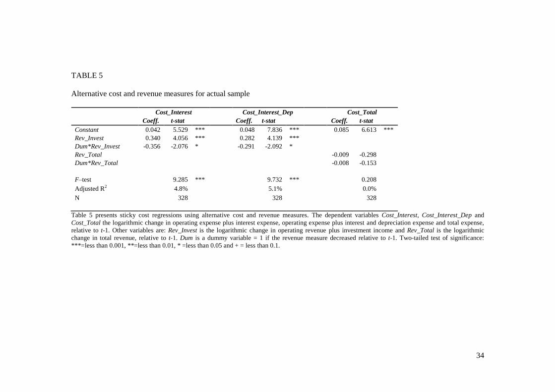
Table 5 reports regressions on the actual sample using alterative cost and

revenue measures. When we include interest costs, depreciation and compare

relative to operating revenue plus investment income, costs are still associated

with revenue and asymmetric. However, changes in total costs are not

associated with changes in total revenue. As the difference is predominantly

due to impairments and asset revaluations, it suggests that such changes are

not related to revenue.

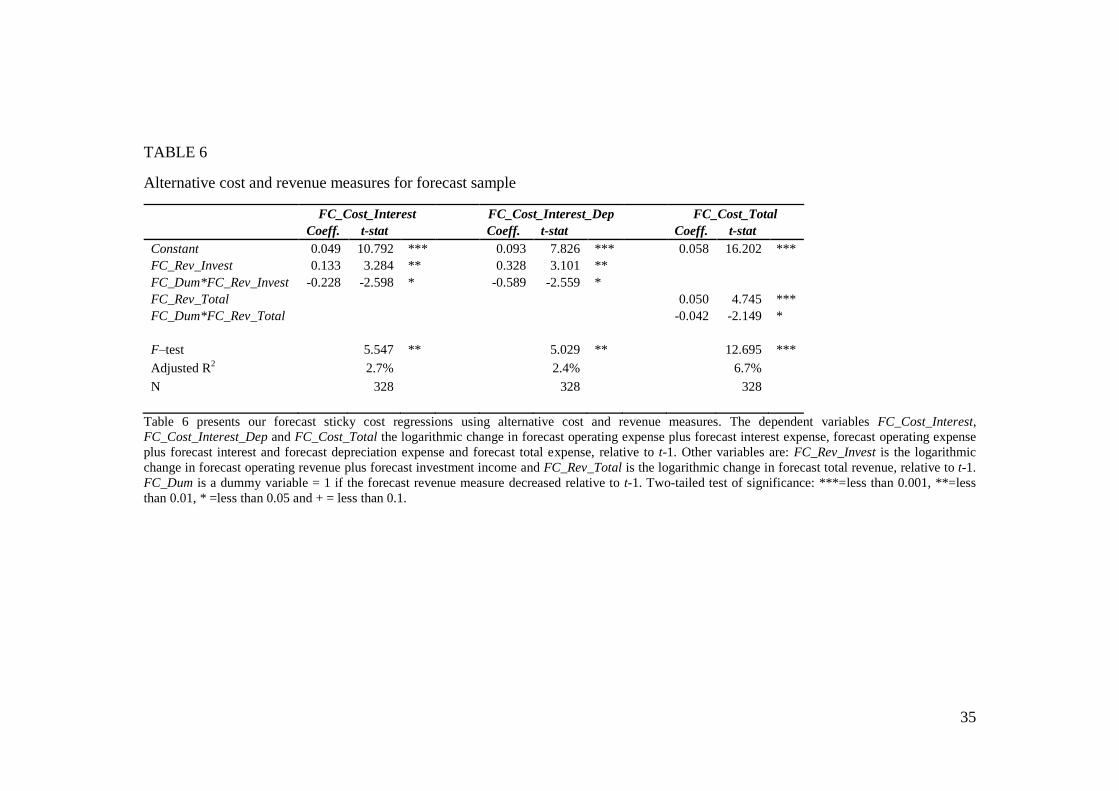
Using alternative measures of cost and revenue for forecast data (see

Table 6) produces similar results to the main analysis. In addition, total cost

and total revenue are significantly associated and managers forecast total costs

to be sticky relative to total revenues. One reason for this is that asset

revaluations and impairments are by their nature typically not forecast. The

alternative cost and revenue measures are also robust to the inclusion of other

variables and robustness tests outlined below.

[Insert Table 5 and 6 about here]

13

An alternative is that forecasts for three years out are simple extrapolations from forecast

assumptions.

23

Alternative tests: Differences in absolute forecast error

One potential criticism is that forecasts may be systematically biased and our

tests capture an artifact in the data rather than forecast cost stickiness. To

alleviate this concern, we conduct an alternative test on whether managers

understand asymmetric cost behavior. Specifically, if managers forecast

asymmetric cost behavior, we would expect the absolute difference between

actual and forecast costs to be no different in years where revenue increases as

opposed to decrease. We calculate our variable of interest for these tests as the

absolute difference between actual and forecast costs in year t, scaled by

actual costs. We find not significant differences for absolute forecast error

depending on whether revenue increased or decreased from the previous year.

This result is unchanged across our alternative revenue and cost measures

outlined above. Therefore, we find evidence consistent with our main results

of managers being equally good at forecasting when revenue increases or

decreases and thus incorporating cost behavior into forecasts.

[Insert Table 7 about here]

Additional tests: Robustness tests

Cheng, Jiang, and Zeng (2012) find that costs of smaller firms decrease more

when revenue falls than they increase when costs rise. Therefore, we split the

sample based on local government size (total assets and population) and type

(district or city). These results are qualitatively similar results (untabulated) to

Model 1 for both the actual and forecast samples. We also rerun the actual

24

sample over a longer time period of 2003-2012. The main inferences, that

costs are asymmetrically related to revenues, are robust to the longer time

period. However, the election year variables (ElectYr*Rev and

ElectYr*Dum*Rev) are no longer significant. This suggests that although

impending elections impact forecast data they have no effect on impact on

actual cost behavior. However, we note that this result is driven by the period

before LTCCPs, it suggests that LTCCP are effective in promoting financial

accountability in the local government setting.

We also control for factors that may drive costs in a local government

setting. Specifically, change in population and income levels (from the 2007

Census) are not associated with changes in costs. Including year fixed effects

does not change the main inferences, although Rev*Dum and

FC_Rev*FC_Dum are only significant at the 10% level (one-tailed tests). The

year fixed effects suggest there are time patterns in the data, however, such

patterns are better explained by electoral year variables, as outlined in Section

4.4.

A further robustness test is to controlling for the magnitude revenue

change. Due to the small sample size there is not enough statistical power to

analyze the effect of changes above 10% (the level used in Calleja et al. 2006).

However, the magnitude of the change in forecast does moderate the size of

the result found in Table 3, although we cannot examine the magnitude of

negative changes in forecast (there are only 44 forecasts for a decrease in

revenue).

25

5. Conclusions

Local government in New Zealand is required to report audited annual reports

following sector neutral accounting standards. Furthermore, they must report

Long Term Council Community Plans containing disaggregated forecast data.

As all local governments must produce forecast data, this provides a strong

setting to examine whether cost stickiness is incorporated into forecasts. We

first find that costs are associated with revenue in a local government setting

and that the relation between costs and revenues seems weaker in local

government than the corporate sector. Furthermore, costs are not only sticky,

but increase even when revenues decrease, albeit at a slower rate. Weak cost

control is consistent with local governments having less incentives to change

costs, especially during revenue downturns. Next, we test whether managers

incorporate asymmetric cost behavior into forecasts. We find similar results to

the actual data, as there is a relation between forecast costs and revenue and

that local governments forecast costs to increase even when revenues are

forecast to decrease. This suggests managers understand the relation between

costs and revenue during downturns and b) local governments have incentives

to increase spending even during downturns.

Overall, our results contribute to the cost stickiness literature by

showing that costs are asymmetric in the local government sector and

managers understand both underlying and asymmetric cost behavior. This is

26

an important contribution to the accounting literature as it demonstrates that

managers understand ‘sticky’ costs as they incorporate asymmetric cost

behavior into forecasts. However, we also observe that costs increase

regardless of the directional change in revenue. This suggests that local

governments either have weak cost controls or have incentives to maintain

expenditure related to ‘social contracts’. The ‘social contract’ explanation is

further supported by the results that electoral cycles (social contract

incentives) impact the forecast and actual relation between cost and revenue.

27

References

Anderson, M., R. Banker, and S. Janakiraman. 2003. Are selling, general and

administrative costs “sticky”? Journal of Accounting Research 41 (1):

47–64.

Anderson, M., R. Banker, R. Huang, and S. Janakiraman. 2007. Cost behavior

and fundamental analysis of SG&A costs. Journal of Accounting,

Auditing and Finance 22 (1): 1–28.

Anderson, M., C. Chen, and S. Young. 2005. Sticky costs as competitive

response: Evidence on strategic cost management at Southwest

Airlines. Working paper, Rice University.

Baber, W. 1994. The influence of political competition on governmental

reporting and auditing. Research in Governmental and Nonprofit

Accounting 8: 109–27.

Balakrishnan, R., M. Peterson, and N. Soderstrom. 2004. Does capacity

utilization affect the “stickiness” of cost? Journal of Accounting,

Auditing and Finance 19 (3): 283–99.

Balakrishnan, R., and T. Gruca. 2008. Cost stickiness and core competency: a

note. Contemporary Accounting Research 25 (4): 993–1006.

Balakrishnan, R., E. Labro, and N. Soderstrom. 2011. Cost structure and

sticky costs. Working paper, University of Iowa.

Banker, R., and L. Chen. 2006. Predicting earnings using a model of cost

variability and cost stickiness. The Accounting Review 81 (1): 285

–307.

Banker, R., D. Byzalov, and L. Chen. 2013a. Employment protection

legislation, adjustment costs and cross-country differences in cost

behavior. Journal of Accounting and Economics 55 (1): 111–27.

Banker, R., S. Basu, D. Byzalov, and J. Chen. 2013b. The confounding effect

of cost stickiness in conservatism research. Working paper, Temple

University.

Banker, R., S. Basu, D. Byzalov, and J. Mashruwala. 2014. The moderating

effect of prior sales changes on asymmetric cost behavior. Journal of

Management Accounting Research (forthcoming).

Baskerville, R., and M. Bradbury. 2008. The NZ in NZ IFRS: Public benefit

entity amendments. Australian Accounting Review 18 (3): 185–90.

Beyer, A., D. Cohen, T. Lys, and B. Walther. 2010. The financial reporting

environment: Review of the recent literature. Journal of Accounting

and Economics 50 (2–3): 296–343.

Bradbury, M., and T. van Zijl. 2006. Due process and the adoption of IFRS in

New Zealand. Australian Accounting Review 16 (3): 86–94.

Bradbury, M., and T. Scott. 2013. The association between accounting and

constituent response in political market. Working paper, University of

Auckland.

Bushee, B. 1998. The influence of institutional investors on myopic R&D

investment behavior. The Accounting Review 73 (3): 305–33.

28

Calleja, K., M. Steliaros, and D. Thomas. 2006. A note on cost stickiness:

some international comparisons. Management Accounting Research 17

(2): 127–40.

Chen, C. X., H. Lu, and T. Sougiannis. 2012. The agency problem, corporate

governance, and the asymmetrical behavior of selling, general, and

administrative costs. Contemporary Accounting Research 29 (1): 252

–82.

Cheng, S., W. Jiang, and Y. Zeng. 2012. Cost Stickiness in Large Versus

Small Firms. Working paper, University of Maryland.

Cooper, R., and R. Kaplan. 1992. Activity based cost systems: Measuring the

cost of resource usage. Accounting Horizons 6: 1–13.

de Madeiros O., and P. Costa. 2004. Cost stickiness in Brazilian firms.

Working paper, Universidade de Brasilia.

Dalla Via, N., and P. Perego. 2013. Sticky cost behaviour: evidence from

small and medium sized companies. Accounting and Finance

(forthcoming).

Feroz, E., and E. Wilson. 1994. Financial accounting measures and mayoral

elections. Financial Accountability and Management 10 (3): 161–74.

Financial Reporting Standards Board. 1993. Statement of Concepts for

General Purpose Financial Reporting, Wellington, NZ: Institute of

Chartered Accountants of New Zealand.

Hirst, D., L. Koonce, and S. Venkataraman. 2007. How disaggregation

enhances the credibility of management earnings forecasts. Journal of

Accounting Research 45 (4): 811–37.

Hirst, D., L. Koonce, and S. Venkataraman. 2008. Management earnings

forecasts: a review and framework. Accounting Horizons 22 (3): 315

–38.

Holzhacker, M., R. Krishnan, M. Mahlendorf. 2014. The impact of changes in

regulation on cost behavior. Contemporary Accounting Research

(forthcoming).

Ingram, R., and R. Copeland. 1981. Municipal accounting information and

voting behavior. The Accounting Review 56 (4): 830–43.

Kama, I., and D. Weiss. 2013. Do earnings targets and managerial incentives

affect sticky costs? Journal of Accounting Research 51 (4): 201–24.

Kido, N., R. Petacchi, and J. Weber. 2012. The influence of elections on the

accounting choices of government entities. Journal of Accounting

Research 50 (2): 443–76.

Krishnan, R., M. Yetman and R. Yetman. 2006. Expense misreporting in

nonprofit organizations. The Accounting Review 81 (2): 399–402

Local Government Act of New Zealand. 2002.

http://www.legislation.govt.nz/act/public/2002/0084/latest/DLM1708

3.html.

Lowry, R., J. Alt, and Ferree, K. 1998. Fiscal policy outcomes and electoral

accountability in American states. The American Political Science

Review 92 (4), 759-774.

29

Niemi, R., H. Stanley, and R. Vogel. 1995. State economies and state taxes:

Do voters hold governors accountable? American Journal of Political

Science 39 (4), 936-57.

Noreen, E., and N. Soderstrom. 1994. Are overhead costs strictly proportional

to activity volume? Journal of Accounting and Economics 17 (1–2):

255–78.

Pallot, J. 2001. A decade in review: New Zealand’s experience with resource

accounting and budgeting. Financial Accountability and Management

17 (4): 383–400.

Pallot, J., and I. Ball. 1996. Resource accounting and budgeting: The New

Zealand experience. Public Administration 74 (3): 527–41.

Penman, S. 1980. An empirical investigation of the voluntary disclosure of

corporate earnings forecasts. Journal of Accounting Research 18 (1):

132–60.

Orsman, B. 2014. Major cuts in Auckland Council's 10-year budget. New

Zealand Herald, 7th

of July 2014.

Skinner, D. 1994. Why firms voluntarily disclose bad news. Journal of

Accounting Research 32 (1): 38–60.

Skinner, D. 1997. Earnings disclosures and stockholder lawsuits. Journal of

Accounting and Economics 23 (3): 249–82.

Subramaniam, C., and M. Weidenmier. 2003. Additional evidence on the

behavior of sticky costs. Working paper, Texas Christian University.

Weiss, D. 2010. Cost behavior and analysts’ earnings forecasts. The

Accounting Review 85 (4): 1441–71.

30

TABLE 1

Sample descriptive statistics

Variables Mean SD Min p25 p50 p75 Max

Actual sample

Operating Expense 47,748 57,096 5,061 18,045 34,037 53,178 455,763

Operating Revenue 52,660 59,435 5,217 21,482 38,360 62,174 509,862

Cost 0.056 0.090 -0.334 0.005 0.055 0.098 0.436

Rev 0.043 0.087 -0.256 0.003 0.044 0.085 0.352

Dum 0.238

Forecast sample

FC Operating Expense 45,178 54,783 3,873 15,969 28,449 52,411 408,340

FC Operating Revenue 54,422 60,507 5,051 20,643 37,922 64,961 502,480

FC_Cost 0.058 0.075 -0.154 0.021 0.038 0.066 0.601

FC_Rev 0.066 0.103 -0.414 0.029 0.060 0.103 0.553

FC_Dum 0.155

Other

Total Assets 1,131,092 1,342,498 52,350 393,791 770,703 1,258,624 9,660,995

Total Liabilities 84,107 122,376 1,624 13,711 36,572 104,624 923,923

Table 1 presents sample descriptive statistics. Operating Expense and Operating Revenue are as reported in the annual at year t in NZ thousands of dollars.

Cost, is the logarithmic change in operating expense relative to t-1, Rev is the logarithmic change in operating revenue relative to t-1, Dum is a dummy

variable = 1 if operating revenue decreased relative to t-1, PriorRev is the logarithmic change in operating revenue in t-1 relative to t-2, , our sticky cost

regressions. FC Operating Expense and FC Operating Revenue are the forecasts as reported in the LTCCP in NZ thousands of dollars. FC_Cost, is the

logarithmic change in forecast operating expense relative to actual operating expense at t-1, FC_Rev is the logarithmic change in forecast operating revenue

relative to actual operating revenue at t-1, FC_Dum is a dummy variable = 1 if forecast operating revenue decreased relative to actual operating revenue at

t-1. Total Assets and Total Liabilities are as reported in the annual at year t in NZ thousands of dollars

31

TABLE 2

Actual sample regressions

Dependent variable = Cost

Model 1

Model 2

Model 3

Model 4

Coeff. t-stat

Coeff. t-stat

Coeff. t-stat

Coeff. t-stat

Constant 0.034 4.462 *** 0.038 4.278 ***

0.042 4.455 ***

0.068 1.466

Rev 0.357 4.305 ***

0.325 3.590 ***

0.366 4.434 ***

0.350 4.194 ***

Dum*Rev -0.395 -2.271 *

-0.455 -2.430 *

-0.429 -2.377 *

-0.392 -2.238 *

Dum

-0.015 -0.868

PriorRev

-0.052 -0.645

PriorDum*PriorRev

0.404 2.175 *

AssetInt

-0.012 -0.739

LiabInt

-0.001 -0.163

F–test

10.262 ***

7.087 ***

6.890 ***

5.248 ***

Adjusted R

2

5.4%

5.3%

7.9%

4.9%

N

328

328

328

328

Table 2 presents sticky cost regressions for the actual sample. The dependent variable Cost, is the logarithmic change in operating expense relative to t-1.

Other variables are: Rev is the logarithmic change in operating revenue relative to t-1, Dum is a dummy variable equal to one if Rev is negative, PriorRev is

the logarithmic change in operating revenue in t-1 relative to t-2, PriorDum a dummy variable equal to one when the operating revenues for period t-1 have

decreased relative to t-2 and 0 otherwise, AssetInt is the logarithm of total assets divided by operating revenue and LiabInt is the logarithm of total liabilities

divided by operating revenue. Two-tailed test of significance: ***=less than 0.001, **=less than 0.01, * =less than 0.05 and + = less than 0.1.

32

TABLE 3

Forecast sample regressions

Dependent variable = FC_Cost

Model 1

Model 2

Model 3

Model 4

Coeff. t-stat

Coeff. t-stat

Coeff. t-stat

Coeff. t-stat

Constant 0.040 6.435 *** 0.035 5.019 *** 0.054 5.846 *** 0.023 0.594

FC_Rev 0.210 3.904 ***

0.242 4.234 ***

0.224 3.660 *** 0.208 3.847 ***

FC_Dum*FC_Rev -0.323 -2.813 **

-0.252 -2.053 *

-0.389 -2.765 ** -0.317 -2.749 **

FC_Dum

0.025 1.624

FC_PriorRev

-0.099 -1.417

FC_PriorDum*FC_PriorRev

0.304 1.929 +

AssetInt

0.006 0.470

LiabInt

0.003 0.603

F–test

7.648 ***

6.004 ***

4.226 **

3.943 **

Adjusted R2

3.9%

4.4%

4.8%

4.7%

N

328

328

257

328

Table 3 presents sticky cost regressions for the forecast sample. The dependent variable FC_Cost, is the logarithmic change in forecast operating expense

relative to t-1, Other variables are: FC_Rev is the logarithmic change in forecast operating revenue relative to t-1, FC_Dum is a dummy variable equal to

one if FC_Rev is negative, FC_PriorRev is the logarithmic change in forecast operating revenue in t-1 relative to t-2, FC_PriorDum a dummy variable

equal to one when the forecast operating revenues for period t-1 have decreased relative to t-2 and 0 otherwise, AssetInt is the logarithm of total assets

divided by operating revenue, LiabInt is the logarithm of total liabilities divided by operating revenue. Two-tailed test of significance: ***=less than 0.001,

**=less than 0.01, * =less than 0.05 and + = less than 0.1.

33

TABLE 4

Sensitivity to the electoral cycle

Dependent variable = Cost Dependent variable = FC_Cost

Model 1 Model 2

Coeff. t-stat

Coeff. t-stat

Constant 0.037 5.020 *** Constant 0.043 7.067 ***

Rev 0.415 5.037 ***

FC_Rev 0.289 5.200 ***

Dum*Rev -0.548 -3.229 **

FC_Dum*FC_Rev -0.494 -3.603 ***

ElectYr*Rev -0.464 -3.285 **

FC_3*FC_Rev -0.329 -4.206 ***

ElectYr*Dum*Rev 2.108 4.980 ***

FC_3*FC_Dum*FC_Rev 0.555 3.124 **

F–test

12.468 ***

F–test

8.964 ***

Adjusted R2

12.3%

Adjusted R

2

8.9%

N

328

N

328

Table 4 presents sensitivity of results to the electoral cycle. For the actual sample the dependent variable Cost, is the logarithmic change in operating

expense relative to t-1. Other variables are: Rev is the logarithmic change in operating revenue relative to t-1, Dum is a dummy variable equal to one if Rev

is negative. For the forecast variables similar variables are estimated and labeled with the prefix FC_. ElectYr is a dummy variable if it is an election year

(2004, 2007 or 2010) and 0 otherwise. FC_3 is a dummy variable = 1 if the forecast is the third year in the LTCCP planning cycle (2009 and 2012) and 0

otherwise. Two-tailed test of significance: ***=less than 0.001, **=less than 0.01, * =less than 0.05 and + = less than 0.1.

34

TABLE 5

Alternative cost and revenue measures for actual sample

Cost_Interest Cost_Interest_Dep Cost_Total

Coeff. t-stat

Coeff. t-stat

Coeff. t-stat

Constant 0.042 5.529 *** 0.048 7.836 *** 0.085 6.613 ***

Rev_Invest 0.340 4.056 ***

0.282 4.139 ***

Dum*Rev_Invest -0.356 -2.076 *

-0.291 -2.092 *

Rev_Total

-0.009 -0.298

Dum*Rev_Total

-0.008 -0.153

F–test

9.285 ***

9.732 ***

0.208

Adjusted R

2

4.8%

5.1%

0.0%

N

328

328

328

Table 5 presents sticky cost regressions using alternative cost and revenue measures. The dependent variables Cost_Interest, Cost_Interest_Dep and

Cost_Total the logarithmic change in operating expense plus interest expense, operating expense plus interest and depreciation expense and total expense,

relative to t-1. Other variables are: Rev_Invest is the logarithmic change in operating revenue plus investment income and Rev_Total is the logarithmic

change in total revenue, relative to t-1. Dum is a dummy variable = 1 if the revenue measure decreased relative to t-1. Two-tailed test of significance:

***=less than 0.001, **=less than 0.01, * =less than 0.05 and + = less than 0.1.

35

TABLE 6

Alternative cost and revenue measures for forecast sample

FC_Cost_Interest FC_Cost_Interest_Dep FC_Cost_Total

Coeff. t-stat

Coeff. t-stat

Coeff. t-stat

Constant 0.049 10.792 *** 0.093 7.826 *** 0.058 16.202 ***

FC_Rev_Invest 0.133 3.284 **

0.328 3.101 **

FC_Dum*FC_Rev_Invest -0.228 -2.598 *

-0.589 -2.559 *

FC_Rev_Total

0.050 4.745 ***

FC_Dum*FC_Rev_Total

-0.042 -2.149 *

F–test

5.547 **

5.029 **

12.695 ***

Adjusted R2

2.7%

2.4%

6.7%

N

328

328

328

Table 6 presents our forecast sticky cost regressions using alternative cost and revenue measures. The dependent variables FC_Cost_Interest,

FC_Cost_Interest_Dep and FC_Cost_Total the logarithmic change in forecast operating expense plus forecast interest expense, forecast operating expense

plus forecast interest and forecast depreciation expense and forecast total expense, relative to t-1. Other variables are: FC_Rev_Invest is the logarithmic

change in forecast operating revenue plus forecast investment income and FC_Rev_Total is the logarithmic change in forecast total revenue, relative to t-1.

FC_Dum is a dummy variable = 1 if the forecast revenue measure decreased relative to t-1. Two-tailed test of significance: ***=less than 0.001, **=less

than 0.01, * =less than 0.05 and + = less than 0.1.

36

TABLE 7

Alternative test of whether managers understand asymmetric costs (increases in revenue – decreases in revenue)

Dum Dum_Rev_Invest Dum_Rev_Total

Mean Diff. t-stat z-score Mean Diff. t-stat z-score Mean Diff. t-stat z-score

Diff_Cost 0.006 0.610 0.429

Diff_Cost_Interest

-0.003 -0.310

-0.508

Diff_Cost_Interest_Dep

-0.005 -0.673

-0.792

-0.017 -1.388

-0.663

Diff_Cost_Total

Table 7 presents alternative univariate tests on whether managers forecast sticky cost. We report Student t-stats and Mann-Whitney U z-scores for

continuous variables. Diff_Cost, Diff_Cost_Interest, Diff_Cost_Interest_Dep and Diff_Cost_Total are the absolute difference between the actual and

forecast operating expense, operating expense plus interest expense, operating expense plus interest and depreciation expense and total expense scaled by

the actual cost number for year t. Dum, Dum_Rev_Invest, Dum_Rev_Total are dummy variables equal to one if the logarithmic change in operating revenue,

operating revenue plus investment income or total revenue, is negative relative to t-1.Two-tailed test of significance: ***=less than 0.001, **=less than

0.01, * =less than 0.05 and + = less than 0.1.