Kristján Páll Pétursson

Investigation of the Influence of Different Generation Types on Islanding Security Region

Master 's Thesis, October 2009

Kristján Páll Pétursson

Investigation of the Influence of Different Generation Types on Islanding Security Region

Master 's Thesis, October 2009

2

Investigation of the Influence of Different Generation Types on Islanding Security Region,

Author(s): Kristján Páll Pétursson Supervisor(s): Yu Chen, PhD Student, CET, DTU. Zhao Xu, Associate Professor, CET, DTU. Jacob Østergaard, Professor, Head of CET, DTU.

Department of Electrical Engineering Centre for Electric Technology (CET) Technical University of Denmark Elektrovej 325 DK-2800 Kgs. Lyngby Denmark www.elektro.dtu.dk/cet Tel: (+45) 45 25 35 00 Fax: (+45) 45 88 61 11 E-mail: cet@elektro.dtu.dk

Release date:

October 2009

Class:

1 (offentlig)

Edition:

1. udgave

Comments:

This report is a part of the requirements to achieve Master of Science in Engineering (MSc) at Technical University of Denmark. The report represents 30 ECTS points.

Rights:

© Kristjan Petursson, 2009

3

ABSTRACT

In the recent years, there has been a rapid growth in distributed generators, increasing the overall penetration in the distribution grid. This has caught the interest of researchers, policy makers, energy planers and others in the islanding operation. The objective of this project is to investigate the influence of different generation types on the islanding security reagion. Within the project the definition of islanding operation is discussed and the critera for successful islanding are considered. The influence of different generation types in the islanding security region is evaluated by theory and simulation with respect to a reference system. Also the influence of load shedding control scheme and Demand as Frequency Reserve (DFR) are investigated. A program code is developed to assist with the analysis of the ISR and graphically show the region of secure islanding and the influences of different generation type.

5

7

TABLE OF CONTENT

Abstract ........................................................................................................................... 3

List of figures ................................................................................................................... 9

List of tables .................................................................................................................. 11

Abbreviations ................................................................................................................ 13

1 Introduction ........................................................................................................... 15 1.1 Background ...................................................................................................... 15 1.2 Problem Formulation ....................................................................................... 15 1.3 Methods and Limitations ................................................................................. 16

2 Theory ..................................................................................................................... 19 2.1 Introduction ...................................................................................................... 19 2.2 Electric Power System ..................................................................................... 19 2.3 Definition of Island and Islanding Transition .................................................. 21 2.4 The Islanding Security Region (ISR) ............................................................... 28 2.5 Reference Island Model ................................................................................... 34 2.6 Different Generation Types.............................................................................. 38 2.7 Study of ISR Criteria ........................................................................................ 39 2.8 Different Combination of Conventional Generators ........................................ 51 2.9 Demand as Frequency Reserve ........................................................................ 52 2.10 Load Shedding .............................................................................................. 56 2.11 Part Conclusion ............................................................................................ 58

3 Programming for ISR Analysis ............................................................................ 59 3.1 Introduction ...................................................................................................... 59 3.2 DIgSILENT Power Factory ............................................................................. 59 3.3 ISR Evaluation Script Problems ...................................................................... 61 3.4 Part conclusion ................................................................................................. 68

4 Simulation Results ................................................................................................. 69 4.1 Introduction ...................................................................................................... 69 4.2 ISR: For the Reference Island Model............................................................... 69 4.3 ISR: For Different Generator Inertia ................................................................ 71 4.4 ISR: Different Prime Mover Time Constant .................................................... 74

Table of content

8

4.5 ISR: For Different Droop Settings .................................................................... 76 4.6 Influence of DFR .............................................................................................. 79 4.7 Different Combination of Conventional Generators ........................................ 80 4.8 Load Shedding .................................................................................................. 82 4.9 Part Conclusion ................................................................................................. 84

5 Conclusion .............................................................................................................. 85

References ...................................................................................................................... 87

A Matlab ISR Source code and functions ................................................................... 89

B Power Factory ISR Source Code ............................................................................ 105

C Component Details for the PF demo model .......................................................... 119

D Matlab Calculations and Scripts ............................................................................ 143

E Contents of Attached CD ........................................................................................ 151

9

LIST OF FIGURES

Figure 2-1: Elements of a power system.[3] .................................................................. 20

Figure 2-2: Facility Island, switch CB1 open for islanding operation. ......................... 23

Figure 2-3: Lateral Island, Switch RC1 open for islanding operation. .......................... 24

Figure 2-4: Circuit Island, CB2 is open for islanding operation ................................... 25

Figure 2-5: Substation Bus Island, breaker CB5 and section breaker CB3 are open for islanding mode. ....................................................................................... 26

Figure 2-6: Substation Island, CB4 and CB5 are open for islanding operation. ........... 27

Figure 2-7: Example of ISR. .......................................................................................... 29

Figure 2-8: Program flow chart for developing ISR in Power Factory[1]. ................... 30

Figure 2-9: Control mechanisme for intentional islanding transition [1]. ..................... 32

Figure 2-10: Original Island model. .............................................................................. 35

Figure 2-11: The reference island model, used for analyzing the ISR region ............... 36

Figure 2-12: Example droop control for the 2 generators in the island model. ............. 40

Figure 2-13: Example of theoretical ISR region for an example system, based only on steady state frequency limits fmin = 49,8Hz and fmax =50,2Hz. ................ 43

Figure 2-14: Scenario 1: Simplified island with power import before islanding .......... 43

Figure 2-15: Scenario 2: Simplified island with power export before islanding ........... 44

Figure 2-16: Simplified block model of the system to analyse frequency behavior at islanding transition ............................................................................. 46

Figure 2-17: Block model from Figure 2-16 rotated to directly analyse frecuency as a function of power mistmatch at islanding. .................................... 46

Figure 2-18: Frequency response at islanding, with with 3 different of droop settings(R). ............................................................................................................ 48

Figure 2-19: Frequency response at islanding, with with 3 different of inertia of generators(H). ................................................................................................... 49

Figure 2-20: Frequency response at islanding, with with 3 different prime mover time constants(Ta). ..................................................................................... 50

List of figures

10

Figure 2-21: Example of theoretical ISR region for the reference system, based only on only frequency derivative criterion (max df/dt = 2,5) .............................. 51

Figure 2-22: Illustration of how the dispatched power of the two machines in the reference model can be offset. ......................................................................... 52

Figure 2-23: Sudden load change and influence on grid dependent on different types of DFR.[15] .................................................................................................. 55

Figure 2-24: Reference island with DFR load. .............................................................. 56

Figure 3-1: Example of how basic ISR parameter values can be changed. ................... 60

Figure 3-2: PF ISR script for analyzing the influence of different generator types. ...................................................................................................................... 62

Figure 3-3: Flow chart for Matlab program, development of ISR curve. ...................... 64

Figure 4-1: ISR for the reference island model (plot also includes each simulation instance, whether it is successful or unsuccessful transition). ............. 70

Figure 4-2: Frequency for two simulation instances on the reference model ................ 71

Figure 4-3: ISR for the reference model with variousinertia. ........................................ 72

Figure 4-4: ISR for the reference model with variousinertia (on top view). .................. 72

Figure 4-5: ISR for the reference model with variousinertia with focus on smaller ISR area. .................................................................................................... 73

Figure 4-6: ISR for the reference model with prime mover time constants. .................. 74

Figure 4-7: ISR for the reference model with various prime mover time constants. ................................................................................................................ 75

Figure 4-8: Frequency plot at islanding for various prime mover time constants. ................................................................................................................ 76

Figure 4-9: ISR for the reference model with various droop control settings. ............... 77

Figure 4-10: ISR for the reference model with various droop control settings. ............. 78

Figure 4-11: ISR for the reference model with DFR implemented. ............................... 79

Figure 4-12: ISR for the reference model with DFR implemented. ............................... 80

Figure 4-13: Different combinations of Conventional Generators. ............................... 81

Figure 4-14: Different combinations of Conventional Generators. ............................... 81

Figure 4-15: ISR for the reference model with two different load shedding implimentations. .................................................................................................... 83

Figure 4-16: ISR for the reference model with two different load shedding implimentations. .................................................................................................... 83

11

LIST OF TABLES

Table 2-1: Typical energy sources, generator types and prime movers. ....................... 20

Table 2-2: Criteria for islanding transition to be considered successful (ISR) .............. 34

Table 2-3: Generators in the referance island model ..................................................... 37

Table 2-4: Transformers in the referance island model. ................................................ 37

Table 2-5: Lines in the referance island model. ............................................................. 37

Table 2-6: Loads in the original island model. .............................................................. 38

Table 2-7: Model and parameters for investigating the influence of different generation on ISR .................................................................................................. 39

Table 2-8: Values used for this example of showing steady state influence of droop control ......................................................................................................... 40

Table 2-9: Potentials for household electricity DFR [13] .............................................. 53

Table 2-10: Comparison of DFR I and DFR II.[14] ...................................................... 54

Table 3-1: Example of the output format from Power Factory ISR scrip. Each column and array extends in both directions. ........................................................ 63

Table 3-2: Matlab functions for Load Simulation Data. ................................................ 65

Table 3-3: Matlab functions for Evaluate ISR. .............................................................. 66

Table 3-4: Matlab functions for Output. ........................................................................ 67

Table 4-1: General simulation parameters. .................................................................... 69

Table 4-2: Parameters to evaluate ISR.with focus on smaller ISR area. ....................... 73

Table 4-3: Simulation parameters for different combination of conventional generators. ............................................................................................................. 80

13

ABBREVIATIONS

Abbreviations Definition

CB Circuit breaker

DPL DIgSILENT Power Factory programming language

DR Distributed Resources

DSO Distribution System Operator

ISR Islanding Security Region

EPS Electric Power System

N.C Normally closed (switch/breaker)

NG3 NextGen Part 3: Control Architecture for Intentional Islanding Operation in Future Distribution Network with High Penetration of Distributed Generation

PF DIgSILENT Power Factory calculation program

RC Recloser

TSO Transmission System Operator

15

1 INTRODUCTION

1.1 Background In the recent years, new types of energy sources are emerging to the market continuously, the proportion of distributed sources is increasing, especially in countries where windpower policies are enforcing increased proportion of windpower production. High penetration of windpower and other Distributed Resources (DR) can give increased challenges in controlling the Electric Power Systems (EPS). Also an increased penetration of DR’s can potentially introduce reliability benefits if it allows for parts of the EPS to be defined as islands, where the islands can then disconnect from the EPS in case of contingencies or maintenance on the EPS outside the defined island. In this way, the customers within the defined island would remain supplied from the DR’s and would potentially experience improved reliability. However, this means that a controller must be in place to handle the transition, where the defined island is disconnected from EPS. In the ongoing project, “NextGen Part 3: Control Architecture for Intentional Islanding Operation in Future Distribution Network with High Penetration of Distributed Generation” (NG3), studies on such controller are being carried out. With the controller in place and a well developed control strategy, this could then potentially improve the reliability of customers within a defined island.

1.2 Problem Formulation This project is about investigating the influence of different generation types on Islanding Security Region (ISR). The islanding security region defines the condition for which, a part of a grid can be islanded from the remaining Electric Power System (EPS) and still supply the customers within the island electric power within acceptable quality limits. This would then potentially improve the reliability for customers within a defined island. Previous analysis on the ISR were made and published in [1]. A program code has been developed to evaluate the ISR curve, for a specified grid model, that defines the

Introduction

16

condition for which the system can safely transition into islanding mode. Further work is being carried out on this subject as well as further studies are being made on the subject of designing a controller for operating the secure transition to islanding mode [2]. The above mentioned work is being carried out in parallel with this project. In the research paper [1], where ISR is proposed, it is assumed that only one generation type is adapted within the defined island. The subject of the project is to investigate the influence of different generation types on the islanding transition operation. To do so, the definition of an island and islanding transition must be defined. The control theory for conventional generators must be studied and the impact of changing some of the characteristic parameters on the islanding process. To be able to analyse influence of the different generation types, the original ISR code must also be adapted for this purpose. Also it is of interest to see if load shedding scheme or the emerging technology Demand as Frequency Reserve (DFR) can improve the ISR conditions. Based on the above, the problem formulation can be summarized into one main problem and 6 subproblems. The main problem:

• Investigation of the Influence of Different Generation Types on Islanding Security Region.

Subproblems:

• Define island and islanding transition. • Study the influence of control parameters. • Study the influence of generator parameters. • Study the influence of prime movers. • Program and adapt the ISR script. • Influence of DFR and Load shedding on ISR.

1.3 Methods and Limitations The methods used in this project are generally as follows. To analyse and explain the theory for the criteria issues regarding the ISR. There will be made simulations on a predefined reference island model, in Digsilent Power Factory (PF). The results from the simulations will be interfaced to Matlab where the simulation analysis will be conducted. The project will conclude from the theory and results of the simulations analysis. A big part of the project is to learn and understand the Digsilent Programming Language (DPL), and to get familiar with the program itself. Also it is clear that when

Introduction

17

analysing the ISR, a lot of data is must be processed. One of the reasons why Matlab was chosen to be used in this project is that it processes data better than PF. The ISR is greatly dependent on the grid layout, implemented control, components and system status, however for this project the analyses are limted to the modified nine-bus system, introduced in [1]. A more detail description of this model will be given in the chapter 2.5. Developing models of different types of DR’s is outside the scope if this project, the models used will be constrained to those available in PF library. However, some models which have been created in previous work, done by others, will be adapted for the ISR simulations. Attached CD holds calculation scripts, models, Matlab files, Power Factory files and more. The full contents list can be viewed in appendix E.

19

2 THEORY

2.1 Introduction The theory which is relevant to this project is introduced in this chapter. As mentioned in the introduction, the idea is to investigate the influence of different types of generation on the ISR. To start off, an introduction is made to the concept and purpose of the ISR and the criteria for successful islanding, as well as a little introduction to power systems. The generation types which are to be investigated will also be introduced and discussed. A method of investigating the influence of different types of DR’s on the ISR will be introduced. Also, the theory behind the ISR criteria will be studied and some examples given. Finally, influence of Demand As Frequency Reserve, load shedding and different combination of generation will be discussed.

2.2 Electric Power System An Electric Power System (EPS) is generally defined as the whole electric grid from the generation of the electric power via power transmission means to the power consumers (loads). Even though originally power systems were DC, today most major transmission systems are three phase AC systems, either 50 Hz or 60 Hz. In this project the focus will be on 50Hz power system even though the same theory will apply for 60 Hz system with some minor adjustments. Figure 2-1 gives an overview of a power system.

Theory

20

Figure 2-1: Elements of a power system.[3]

Power generation is typically produced by the means of one of the following energy sources. These are fossil fuel, kinetic energy of water or wind and nuclear fission. A prime mover (turbine) produces the mechanical energy, from those energy sources, then transfers the mechanical energy to an electric generator. Most common prime movers and generators associated with these types of energy sources can be seen in table 2-1 Energy source Turbine Generator Fossil fuel Steam turbine Synchronous Kinetic energy of water Hydrolic turbine Synchronous Kinetic energy of wind Wind turbine Synchronous or Asynchronous Nuclear fission Steam turbine Synchronous

Table 2-1: Typical energy sources, generator types and prime movers.

Theory

21

Also other sources are available but not as widely adopted. Examples of such, to name a few, are tidal, wave and photovoltaic (solar cells) [4]. The generators in the power system are typically synchronous generators. Also in some cases asynchronous generators are used or even DC generators. DC generators, photovoltaics and other power generators that cannot produce the power fulfilling the grid requirements are typically connected to the power system via power converter. The power converters can then be either DC-AC or AC-DC-AC. The inverter charateristics can be adapted to specific needs but are often designed to immitade the characteristics of the synchronous generator. The power transmission system is classified in three subsystems [5].

• Transmission system. • Subtransmission system. • Distribution system.

Each subsystem operates at specific voltage level. The voltage levels are standardized but vary after specific grid codes. The transmission system is usually 230 kV and above. The transmission system interconnects all the main power plants and main load centers. The transmission system transfers large amount of electric power, from the power plants to the load centers at higher voltage level and by doing so minimizes power losses in the powerlines. The subtransmission system transfers smaller amount of power from the transmission substations to the distribution stations, typically at voltage levels from 69 kV to 138 kV. The distribution system, typically operated at 4 kV to 34,5 kV, transfers the electric power to industrial customers at this voltage level and to low voltage substations that then supply the low voltage customers (0,4 kV).

2.3 Definition of Island and Islanding Transition Islanding is the concept of disconnecting a part of a power system from the remaining power system. The part of the system which is then disconnected is regarded as an island. The island can in theory be a part of a distribution grid, or even more as in distribution grids and an interconnecting subtransmission system or parts of the transmission system. To be able to run the island while disconnected from the main power system it must have some producing units, central unit and/or an aggregation of decentral production units (DR) within the island. The island can then be islanded as a part of planned islanding or during disturbances, for example short circuits, on the main system, therefore contribute to higher reliability for the customers (loads) in the island.

Theory

22

While in island mode the system must maintain stability, frequency limits must be observed as well as voltage limits. However the system does not need to be in synchronism with the main power system while in island mode but before connecting the system again it must be brought back into synchronism. While in island mode the aggregated production in the island must be sufficient to supply the loads which are connected and maintain the system requirements, which is by controlling the frequency and voltage of the island so that it is within required limits as well as ensuring system stability. In cases where the load is higher than the production capabilities of the island, it can be considered to disconnect some of the loads in the island (load shedding). Load shedding scheme should be in place where loads are prioritised and the loads of highest priority should be maintained as long as stability and power quality can be ensured. Types of Islands There can be a many different configurations of islands. In [6] they are categorized into five different configurations, which are as follows:

1. Facility Island. 2. Lateral Island. 3. Circuit Island. 4. Substation Bus Island. 5. Substation Island.

For this project there will be a main focus on a Substation Island allthough the theory and simulations could also be applied to the other types of islanding. The following is a brief description of the island types in the order as presented above.

Theory

23

2.3.1 Facility Island This type of island describes an island where the load and DR are served within the same facility. This could for example be a production facility running their own generator in parallel with the EPS. In case of outage of the power system, the facility can be selfsufficient with their DR. An example of a facility island is shown in Figure 2-2.

Figure 2-2: Facility Island, switch CB1 open for islanding operation.

Theory

24

2.3.2 Lateral Island A lateral island has DR generation feeding in on the lateral and can serve the lateral loads while islanded. Reason for islanding can be EPS outage or to decrease load on the circuit (and EPS), having the lateral generating units providing for the lateral loads, see Figure 2-3. It should be noted that the lateral loads are not shown on the figure but should be assumed to be further down the lateral, outside the boundaries of the figure.

Figure 2-3: Lateral Island, Switch RC1 open for islanding operation.

Theory

25

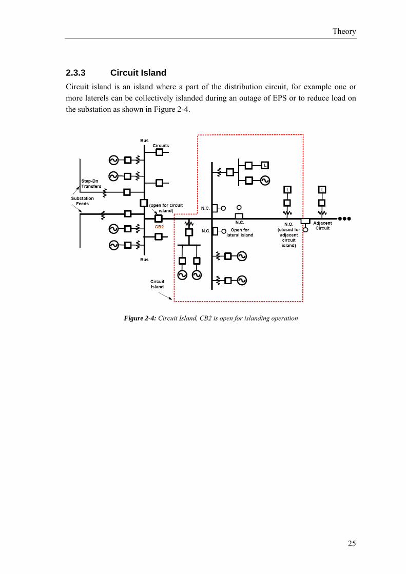
2.3.3 Circuit Island Circuit island is an island where a part of the distribution circuit, for example one or more laterels can be collectively islanded during an outage of EPS or to reduce load on the substation as shown in Figure 2-4.

Figure 2-4: Circuit Island, CB2 is open for islanding operation

Theory

26

2.3.4 Substation Bus Island Bus island can be defined as an island where a bus is isolated from other busses in the substation by opening the sectionbreakers and disconnecting the feeding transformer from the bus. This way the bus can be islanded with all its connected loads and DR in case of a feeder or transformer outage or to reduce the load of the bus feeder. See Figure 2-5.

Figure 2-5: Substation Bus Island, breaker CB5 and section breaker CB3 are open for islanding mode.

Theory

27

2.3.5 Substation Island A substation island is an island where the loads are typically served by one substation and a collection of DR. The substation can then disconnect from the feeding transformer, effectly putting the substation with its loads in island mode. This can be done in case of EPS outage or to reduce load on the substation feeder transformers or any overlying elements. This type of island is most similar to the one that will be used for analysis in this project. An example of substation island can be seen in Figure 2-6.

Figure 2-6: Substation Island, CB4 and CB5 are open for islanding operation.

2.3.6 Considerations When transitioning to island mode, or while in island mode, there are some issues that need to be considered. A number of key considerations are listed in [7] and is also introduced here:

• Possible damage to customer equipment. • Maintenance of the producing units in the island. • Reduced reliability of the EPS to which the island is connected. • Reduced power quality. • Fault detection. • System protection.

Theory

28

• Coordination with load shedding schemes. • Deferral of system improvements (reinforcements). • Voltage regulation.

Many of these considerations are outside the scope of this project and therefore not handled in the report. However it is clear that in case of unsuccessful islanding transition frequency variations or frequency derivatives could cause damage to customer equipment as well as voltage increases or collapses, therefore it is important to know before the islanding transition, if the transition will be successful or not. Also while in island mode, the reliability of the overlying EPS might be reduced as some of the DR, and therefore reserve, is no longer available. While in island mode the source impedance within the island will be higher compared to the source impedance while the island is connected to the EPS, this can then decrease the power quality as it is likely to see more harmonics, depending on the loads in the system. The fault current will be smaller and that can influence the fault detectionIn cases where the fault current is reduced to levels below what is neccisary to trigger the protection elements, then a possible solution could be to have alternate settings for the elements while in island mode. Depending on the types of DR and the available reactive power control the voltage regulation can also become a problem.

2.4 The Islanding Security Region (ISR) To avoid system instability during an islanding transition, the concept of the ISR is proposed in the article [1] as well as a control mechanism. The ISR maps the condition for which an islanding transition can be successfully performed for a pre-defined island. That is the conditions where a part of a grid, for example a substation island (described in chapter 2.3.5) can be disconnected from the feeding transformer and the grid, where as the island can run on DR’s supplying the loads within the island. Whether the islanding transition is successful any island is highly dependent on the load and generation conditions in the grid at the time of transition. For example it is clear that in many cases when the load is much greater than the generation, in the defined island, and there is a sudden or unplanned outage of the feeding grid, it is more likely that a transition to islanding mode will be unsuccessful. This is clear as there will be too little active power available from the DR’s and the mismatch of power will be extracted from the kinetic energy of the generators, resulting in frequency drop. In comparison, if the difference between load and generation is small, or close to zero, it is more likely that the transition will be successful. The success of the transition is highly dependant on the conditions before the transition and the general ability of the defined island to cope after islanding. The regulating response of the DR’s in the grid has a big influence as well as the total inertia. Other factors can also influence transition, most importantly primary control of the DR as well as other load controlling concepts such as load shedding and

Theory

29

or Dynamic Frequency controlled Reserve (DFR), which is a technology still under development (further explained in chapter 2.9). On the other hand, when the islanding is planned, theoretically if any additional DR’s are offline at the time, they can be brought online to increase the reserve in the island and improve the conditions for islanding. This way a better balance between load and generation can be reached before the islanding transition.

2.4.1 The ISR Evaluation Script The ISR can be graphically defined with the ISR evaluation script, as shown in Figure 2-7.

Figure 2-7: Example of ISR.

In the above figure (Figure 2-7), the curve indicates the boundaries for stable transition, however in this case frequency deviation limits are only considered, not derivatives, voltage or other criteria. That is, if the defined island is island loads and generation are within the curve, islanding transition should be successful. The Y-axis indicates how much active power is generated within the island pre-islanding and the X-axis shows the load within the island.

Theory

30

The island model used in this example is the reference model, which is introduced in chapter 2.5. The reason why simulations are done on exactly this system is so that the ISR can be compared to that found in [1], and it is shown to be the same. It should however be noted that the per-unit base values in this example has been redefined. The generation base value is defined as the total rated active power in the island, here 320 MVA and the load base value is defined as total full active load in the system, here 320 MVA. The way the curve in Figure 2-7 is developed in [1] is best described with the flow chart shown in Figure 2-8.

Figure 2-8: Program flow chart for developing ISR in Power Factory[1].

The flow chart above describes how the ISR is evaluated by a programmed script in PF. The first block is a program modification block and this is where the main parameters

Define variables/

inputs

Output results P1, P2, …Pq (Q=1,2,3…)

First loop for gen., P_gen1≥P_gen≤Pgen2

Simulation with islanding operation

Second loop for loads,P_lod1≥P_lod≤P_lod2

Increase gen by x% Pgen_m=Pgen_(m-1)·(1+x%)

(m=1,2,3,…)

Frequency f1≥f≤f2

(in 15sec)

Increase loads by y% Pload_n=Pload_(n-1)·(1+y%)

(n=1,2,3,…)

Record results: Pk(P_load,P_gen),

(k=1,2,3,…)

Yes

No

No

No

Yes

Yes

Theory

31

for the script are set. These parameters are set depending on what ISR range is to be plotted and what resolution should be used, this will also greatly influence the computation time for developing the ISR curve – larger range and higher resolution increase the simulation time.

• P_gen1 & P_gen2 defines the lower and upper limit of the DR power production condition before islanding, respectively.

• P_lod1 & P_lod2 defines the lower and upper limit of the loads condition

before islanding, respectively.

• x% & y% defines the resolution of which the generation and loads are increased by, for each increment(each loop), respectively. Higher resolution will produce curves with higher detail.

The next block is a decision block (outer loop). The first time the script reaches this block, it will set the generation equal to P_gen1, the lower limit. Then for each run of the loop, it will evaluate if the generation is within the limits set in the first block. If the outcome is positive, the script will continue, if it is negative, the script has finished and will output the results. The third block is also a decision block (inner loop). The first time the script reaches this block, it will set the generation equal to P_lod1, the lower limit. Then for each run of the loop, it will evaluate if the load is within the limits set in the first block. If the outcome is positive, the script will continue, if it is negative, the script will return to outer loop and the process is repeated until the outer loop has reached its limit and the script has finished outputting the results. The fourth block is also a decision block, it evaluates if the island fulfills the criterias set for successful islanding. As shown here it only evaluates if the frequency deviation is within limits and if positive it registers the values of P_gen and P_load and then continues to the inner loop. In the process of the project work, there have been made some changes and additions to this script. These are documented in chapter 3. It should also be noted that during the period of this project, the ISR script is being refined and worked on, by others.

Theory

32

2.4.2 Control Mechanism In the article [1], where the ISR is proposed along with a control mechanism, the functionality of the control mechanism is described. The flow chart seen in Figure 2-9 is given, explaining in more detail the performance of the mechanism.

Figure 2-9: Control mechanisme for intentional islanding transition [1].

It is suggested that a central controller unit is to be within the defined island for the monitoring, controlling and islanding processes. The chart shows operation of the controller in three states which the defined island can be in. Either it is in grid connection mode, which is the normal operating conditions, or transition mode, where

Grid connection mode, Real-time

system state moni-tored

Alarm state, with control techniques

Control & coordina-tion scheme search & establish based on PIP

or PEP

No control, or mod-erate control

Perform islanding operation

Post-Islanding transition state

TSO island-ing signal

TSO island-ing signal

System state within ref. ISR

No

Yes

Stage 1: Grid connection mode; Monitoring, super-vision and ISR assessment

Stage 2: Transition mode; Control, Coordination and ISR re-assessment

Stage 3: Islanding mode; Post-islanding transition

No

No

No

Yes Yes

Yes System state within im-proved ISR

Theory

33

the controller establishes whether or not the island is ready for islanding transitions, and finally there is the islanding mode, where the defined island has been been disconnedted from the main grid. Depending on the control scheme, there can be additional controllers involved, for example for load shedding to improve the system state when outside the ISR region. Stage 1, Grid Connection mode: The central controller monitors the production and loads within the defined island. It will continuously compare the system state with the reference ISR, depending on the outcome of whether the system is within the ISR will be ready to take the appropriate action when an islanding signal is received. The islanding signal can be received either due to an outage, contingencies or when a planned islanding occurs. The islanding signals can be received from TSO, DSO or relays indicating the need for islanding. When an islanding signal is received, stage 2 (Transition mode) is initiated. Stage 2, Transition mode: The controller enters transition mode by one of the two paths shown in the flow chart, dependent on the output of the first decision block (system state in stage 1). If the system is within the reference ISR, no control or moderate control is needed and the controller can immidetly procede to stage 3 (island mode). However, if the transition signal is received while the system state is outside of the reference ISR, some control scheme must be activated or the transition is not successful. The control scheme inplace is dependent on the resources available and what kind of control has been implemented in the specific grid, the controller should then chose the most appropriate control action depending on the system state. After the control action, the system state is then evaluated again against the reference ISR and if the system state is improved, and is now within the boundaries of the ISR, then and only then will the controller procede to stage 3 (island mode). Stage 3, Island mode: In this stage, the defined island has been separated from the surrounding grid and should be running autonomously with power supplied to the customers within acceptable quality limits. The proposed control mechanism does not discuss how to reconnect the island again into grid connection mode and this is considered outside of the project scope.

2.4.3 Criteria for ISR The criterion for successful islanding, used to define the ISR is in [1] the frequency deviation. The frequency should be between 49,8 Hz and 50,2 Hz 15 seconds after the

Theory

34

islanding. This criterion will be used in this project, however it is suggested by project supervisor to also include critera for frequency derivative (derivative should be less than 2,5 at any time) and that voltage limits should be between 0,8 pu and 1,2 pu 15 seconds after islanding. The critera for successful islanding, used for the project is summarized in Table 2-2. Criterion Min value Max value Frequency deviation 49,80 Hz 50,20 Hz Frequency derivative -2,50 Hz/s 2,50 Hz/s Voltage 0,80 pu 1,20 pu

Table 2-2: Criteria for islanding transition to be considered successful (ISR)

2.5 Reference Island Model As mentioned previously a reference model will be defined, which will be used throughout this report for simulations and evaluations, with minor adjustments. The island model is introduced in [1] and is a modified version of a demo model found in PF. In this chapter there will be given details about the model, modifications and layout. The original model can be seen in Figure 2-10. This model is included as a demo in the PF software and is designed for the following types of analysis:

• Transient stability calculations. • Impact of different voltage controllers.

Theory

35

Figure 2-10: Original Island model.

In theory, any grid model could be used with the developed ISR evaluation script. How-ever the script is developed with some limitations, for example only synchronous gene-rators are considered. If a different model is to be used, some additional programing would be needed for the ISR script to handle other types of components.

2.5.1 Details of the Original Island Model The island represented in Figure 2-10 is the PF demo model. It is operated at four voltage levels, generation at 16,5kV, 18kV and 13,8kV where as transmission/distribution is at 230kV. Loads and generation are lumped together into few units to give an easy overview of the whole system. The components in the model include many component details for the lines, generators, transformers etc. The component parameters for the original PF grid are listed in C (component specs.). This model is the basis for the model that will be used for analysis of ISR region, the reference islanding model the modifications which weremadeare described in the following chapter.

Theory

36

2.5.2 Reference Islanding Model For simulation purposes, a reference model is introduced. This model is chosen as it is the same as used in [1]. The reference model is a slightly modified version of the 9 bus model mentioned in chapter 2.5.1. The modifications made to the nine bus system, is to imitate a defined island that is connected to an EPS. This island will only have one connection point to the main grid. One of the three generators in Figure 2-10, G1, is replaced by a feeder reprisenting the EPS. An additional line and one bus are also added where the coupling to and from island mode will initiated. The resulting island model can be seen in Figure 2-11.

Figure 2-11: The reference island model, used for analyzing the ISR region

When simulating island mode, the breakers for line 7 are opened, leaving the grid supplied by only the two generators, G2 and G3. The system parameters for the reference island can be seen in Table 2-3 - Table 2-6.

Defined island.

Theory

37

Generator Type Rated Power [MW]

Rated Voltage [kV]

Inertia H [s] Droop Control, R

Prime mover Time constant, Ta [s]

G1 Sync. 192 16,5 4,165 0,02 0,2

G2 Sync. 128 18,0 2,765 0,03 0,2

Table 2-3: Generators in the reference island model

There are three transformerswhich parameters are shown in Table 2-4.

Transformer Rated Power [MVA] Rated HV [kV] Rated LV [kV]

T1 250 230 16,5

T2 200 230 18

T3 108,8 230 13,8

Table 2-4: Transformers in the reference island model.

Transmission lines parameters are given in Table 2-5.

Line Rated Current [kA] Impedance [Ω/km] Susceptance[μS/km]

Line 1 1,000 5,290+j44,965 60,00

Line 2a+b 1,000 16,928+j85,169 150,00

Line 3 1,000 4,4965+j38,088 70,00

Line 4 1,000 6,2951+j53,323 70,00

Line 5 1,000 20,631+j89,83 50,00

Line 6 1,000 8,993+j48,668 50,00

Line 7 1,000 5,290+j44,965 70,00

Table 2-5: Lines in the reference island model.

There are three loads in the grid and are detailed inTable 2-6.

Theory

38

Loads Active Power [MW] Reactive Power [ MVAr]

Load A 120 60

Load B 125 60

Load C 72 36

Table 2-6: Loads in the original island model.

For the ISR simulations in chapter 4, the frequency and voltage will be monitored on bus 8 as done in [1].

2.6 Different Generation Types Distributed resources are typically a combination of energy source, prime mover (turbine), generator and a controller or controllers. The possible combinations of these elements are many and it must be considered impractical to model each type of generation to investigate the influence on the ISR. Therefore it is proposed here that to investigate the influence of different generation types on the ISR, a standard synchronous generator model will be used along with a steam turbine model, which are already integrated in the reference model. By adjusting the parameters on these standard models, we can try to replicate different types of generation to investigate the influence on the ISR. For the turbine, the key parameter will arguably be the time constant. Considering a steamturbine a large time constant can be used to immitade a steamturbine where a large fraction of the mechanical torque produced is supplied by the reheater part of the turbine. A smaller constant will then reprisent a prime mover with smaller or no fraction of the torque produced from a reheater (faster turbine). Even though some of the prime mover characteristics will be lost, it should give a good idea of what the influence of different prime mover types would have on the ISR. For the generator, a model of the synchronous machine can be used and here the parameter is the generator inertia. The inertia is then an indication of the rotational energy stored in the rotating rotor and turbine combined. For the controller, the droop setting will be used as the main parameter. Depending on turbine type, the droop controler is implemented in different ways. Here the focus is on the way proportional part of the controller. The droop characterises how the controller reacts to frequency disturbances in the grid.

Theory

39

By focusing only on these three parameters, the number of simulations and work is limited considerably on the expense of the accuracy of the results. To summuarize, the models used for the general investigation of different generation types, are a steam turbine, synchronous generator and a droop controller. The parameters investigated are the turbine time constant, generator inertia and the droop setting of the power controller, see Table 2-7. Generator Prime mover Power Control

Model used: Synchronous Steam turbine Droop control

Parameter of interest: Inertia (H) Time constant (Ta) Droop (R)

Table 2-7: Model and parameters for investigating the influence of different generation on ISR

2.7 Study of ISR Criteria In Table 2-2, there are defined three criteria for ISR, which are the frequency deviation, frequency derivative and voltage and these will be studied here. It should also be mentioned that system stability should also be considered. The nature of stability problems are in [8], dividet up into three main categories

• Angle stability. • Frequency stability. • Voltage stability.

When the angle stability is considered, the contingencies are divided in two groups, depending on their characteristics. These are small signal- and transient stability contingencies. Small signal contingencies are minor disturbances on the grid, such as small load or generation variations. The transient stability is considered to be when the system is subject to more sever contingencies such as outage of generating unit or short circuit. Therefore an islanding transition should be considered more as transient stability issue. Without going deeper into stability theory the criteria for successful ISR will be studied.

2.7.1 Frequency Deviation The frequency deviation is highly dependant on the droop settings of each generating unit controller within the defined island and the pre-islanding conditions. The droop

Theory

40

percentage R is the difference of min (full load) and max (no load) frequency which can be expected from a synchronous machine with respect to the system frequency (under normal operation), see equation 2.1.

system

loadfullloadno

fff

R __ −= [9] ( 2.1)

Where: R is droop constant. fno_load is frequency at no load [Hz]. ffull_load is frequency at full load [Hz]. fsystem is set point frequency [Hz]. Figure 2-12 shows ideal steady state characteristics of a governor with speed droop. In the following example, data from G2 and G3 in Table 2-3 will be used. The values are summarized in Table 2-8. Generator Rated power [MW] Controller Droop G2 192 0,02 G3 128 0,03

Table 2-8: Values used for this example of showing steady state influence of droop control.

Figure 2-12: Example droop control for the 2 generators in the island model.

Figure 2-12 illustrates the steady state output of generator G2 when subjected to a frequency deviation. The frequency deviation can be, for an example, caused by

Theory

41

generation and load power mismatch after islanding. The calculations can be seen in appendix D. The regulation constant of an islanded system (K) depends on the participation of each producing units in the island. It is related to droop of the units and can be determined for each machine by the equation 2.2. The total regulation constant for the island is the sum of the regulation constants for each machine within the island.

system

rated

fRP

K⋅

= ( 2.2)

Where: R is droop constant. K is regulation constant [MW/Hz] Prated is the rated active power [MW] fsystem is the set point frequency [Hz] For the island model used in the project the regulation constant K of the island can becalculate as an example. For G1, data from Table 2-3 is used:

HzMWKG /19200,5002.0

00,1922 =

⋅=

For G2, data from Table 2-3 is used:

HzMWKG /33,8500,5003.0

00,1282 =

⋅=

Resulting in:

HzMWKKK GGisland /33,27732 =+=

For 1 Hz drop in the frequency a collective increase in power output from the two units

prime mover of 277,33 MW should expected.

When the defined island transitions from grid connection mode to island mode, it can be expected that there is a power mismatch between generation and consumption. The level of mismatch highly depends on pre-transition conditions. Steady state output change for the generating units after transition can be calculated by equations 2.3 and

Theory

42

2.4, if the transition is simply treated as load change, either an increase or decrease of consumption in the island. PPP prePost Δ+= ( 2.3)

islandpostpre KffP ⋅−=Δ )( ( 2.4)

Where: Ppost is the steady state power output after islanding transition, assuming droop control. fpost is the frequency after islanding. Ppre is the dispatched power of the generators before islanding transition. fpre is the frequency before islanding transition. ∆P is the power mismatch immediatly after islanding transition, after steady state is reachedIt is contributed by the droop controllers. Therefore, the steady state post islanding frequency deviation is calculated as follows based on the power mismatch post islanding transition.

island

prepost KPff Δ

−= ( 2.5)

From equation 2.5, the required pre-islanding conditions can be evaluated based on the steady state frequency limits (ISR region based only on steady state frequency). These depend on the limits given in the grid codes of where the ISR would be implemented. In Figure 2-13 gives an example of such ISR limits based on allowed max and min frequency which are 50,2 Hz and 49,8 Hz respectively, these are also the limits used in [1].However according to the nordic grid codes, the frequency should remain within 49.9 Hz – 50,1 Hz for normal operation [10]. Other island values used in this example are those given in Table 2-8. See appendix D for detailed calculations.

Theory

43

Figure 2-13: Example of theoretical ISR region for an example system, based only on steady state

frequency limits fmin = 49,8Hz and fmax =50,2Hz.

Not considered in the above plot is that, depending on the power dispatch of each machine pre-islanding, it is possible that one of the generators have reached their power limits, and would therefore influence the shape of the ISR. The following two scenarios can be used to further illustrate the theoretical steady state frequency after islanding. First example should illustrate a scenario where the defined island is importing power before islanding where as the second example illustrates a scenario where the island is exporting power before islanding.

1. First scenario, Here the power is being importet to the island before islanding transition, shown in Figure 2-14:

Figure 2-14: Scenario 1: Simplified island with power import before islanding

Defined island: Kisland=277,33 MW/Hz G2 G3 Power imported from

external grid, 10MW

Load 106MW

57,6MW 38,4MW

Theory

44

Generators G2 and G3 within the defined island, are producing 57,6 MW and 38,4 MW, respectively, and the total load in the island (including any losses) is 106 MW. This means that the difference of 10 MW is being supplied from the power system before islanding. Assuming 50 Hz grid frequency pre-transition, the post islanding steady state frequency within the island can then be calculated by equation 2.5 to be:

Hzf post 96,4933,277

00,1000,50 =−=

2. Second scenario, Here the power is being exportet from the island before

islanding transition, shown in Figure 2-15:

Figure 2-15: Scenario 2: Simplified island with power export before islanding

Generators G2 and G3 within the island, are producing 57,6 MW and 38,4 MW, respectively, and the total load in the defined island (including any losses) is 80 MW. This means that the difference of 16MW is being supplied from the power system before islanding. Still assuming 50 Hz grid frequency pre-transition, the post islanding steady state frequency within the island can then be calculated with equation 2.5 to be:

Hzf post 06,5033,27700,1600,50 =

−−=

Based on the above it is clear that when the island is exporting power, an increased steady state frequency should be expected post-islanding. Reversely the steady state frequency will be lower post-islanding if the island is importing power pre-islanding.

2.7.2 Frequency derivative Generally a sudden increase or decrease in load or generation will influence the frequency. The larger and faster the change is, the steeper frequency change should be expected (higher derivative). Frequency derivatives are not covered in the Nordic grid

Defined island: Kisland=277,33 MW/Hz G2 G3 Power exported to

external grid, 16MW

Load 80MW

57,6MW 38,4MW

Theory

45

codes, but as suggested by this projects superviser a derivative limit of 2,5 Hz/s should be set as a criterion for successful islanding. The derivative can be defined as follows. From equation (2.6) the effects of imbalance electromagnetic and mechanical torque is described. An expression for frequency derivative as a function of system inertia and change in power can be derived.

emam TTT

dtd

J −==ω

[11] ( 2.6)

c

system

system

EfP

dtdf

⋅

⋅Δ=

2 ( 2.7)

Where: J is combined moment of inertia for generator and turbine [kg·m2] ωm is the angular velocity of the rotor [rad/s] Ta is the accelerating torque [N·m] Tm is the mechanical torque [N·m] Te is the electrical torque [N·m] Esystem is the rotational energy stored in the system (kinetic energy) [MW·s] The rotational energy of the system should include all rotating machines connected directly to the system. The rotating energy in the system can be summed up for each machine as follows:

∑=

⋅=N

iiisystem SHE

1 ( 2.8)

From equations 2.7 and 2.8 it is clear that the frequency derivative is inversely proportional to the rotational energy in the system and proportional to the change in power. Therefore it can be assumed that higher inertia within the island should contribute to lower frequency derivative.

2.7.3 Simplified Model of the Islanding System and Frequency Response To try to realize the influence of the different parameters on the islanding transition response a transfer function of simplified model of the system can be created. In this chapter a much simplified transfer function of an island will be introduced, so that the frequency response of islanding transition can be analysed and compared to the simulation results in later chapter.

Theory

46

The proposed simplified model can be seen in Figure 2-16.

Figure 2-16: Simplified block model of the system to analyse frequency behavior at islanding transition

The block model, in figure 2-16, can be rotated to show the frequency as function of the power mismatch at the time of islanding. From the model, the transferfunction can also be directly derived, see Figure 2-17.

Figure 2-17: Block model from Figure 2-16 rotated to directly analyse frecuency as a function of power mistmatch at islanding.

The transferfunction for the simplified system is therefor as follows:

sHK

sTsHK

sTsHP island

arefisland

aoutout ⋅⋅

⋅⋅⋅+

⋅+⋅⋅

⋅⋅⋅+

⋅Δ−⋅⋅

⋅Δ=Δ2

11

12

11

12

1 ωωω

K_island sTa+1

1

Hs⋅21

Droop control Prime Mover

System inertia

∆ωout

ωref

+

+

+

Power mismatch at islanding

∆P

-

K_island sTa+1

1Hs⋅21

Droop control Prime Mover System inertia

∆ωout ωref

-

+ +

+

Feedback of measured freq (ω)

Power mismatch at islanding

∆P

Theory

47

As the main interested is in the frequency response, due to power mismatch, the reference frequency can be set to zero and the function is thereby simplified. The system frequency can then be superimposed on the response after calculation. The resulting transferfunction can be seen in equation 2.9.

sHK

sT

sHP

islanda

out

⋅⋅⋅⋅

⋅++

⋅⋅=ΔΔ

21

111

21

ω ( 2.9)

Now the frequency response of the simplified system can be analysed with respect to the parameters of main interest. That is the time constant of the prime mover, the regulation constant (derived directly from the droop control) and the system inertia. As basics for the analysis there will be used the same data, as for the previous calculations, which is the same model which will be used for the simulations in chapter 4. Due to the simplifications in this model, developed in this chapter, the analysis does not include many of the parameters that otherwise would influence the system response when islanding. As an example the frequency behavior for an islanding transition can be looked at, where the defined island is in power import mode, and immediatly after islanding there will be a power mismatch of ∆P = -10 MW as indicated in Figure 2-14. Firstly the influence of the droop control can be visualized as shown in Figure 2-18. The calculations are shown in appendix D. Three different droop settings are tested:

1. Droop settings as set in the reference model RG2 = 0,02 and RG3 = 0,03.

2. Increased droop, to 200% , that is RG2 = 0,04 and RG3 = 0,06.

3. Increased droop, to 50% , that is RG2 = 0,01 and RG3 = 0,015.

Theory

48

Figure 2-18: Frequency response at islanding, with with 3 different of droop settings(R).

Figure 2-18 shows that the droop, which is inversely proportional to regulation constant, will greatly influence the steady state frequency. This is also expected as the regulation constant functions as proportional controller. Higher gains will giver faster response and less steady state deviation. Secondly the influence of different inertia can be analysed with this model. Three different inertia values are tested:

1. Inertia as set in the reference model HG2 = 4,125 s and HG3 = 2,765 s.

2. Increased droop, to 200%, that is HG2 = 8,250 s and HG3 = 5,530 s.

3. Decreased droop, to 50%, that is HG2 = 2,063 s and HG3 = 1,383 s.

Theory

49

Figure 2-19: Frequency response at islanding, with with 3 different of inertia of generators(H).

From Figure 2-19 it is clear that increased inertia within the island will decrease the frequency derivative and allow the frequency to settle faster to a steady state. The steady state frequency will be the same for all cases as the regulating constant (Kisland) is the same for all cases. In Table 2-2 critera for frequency derivitative is given and should be lower than 2,5. From the above it is therefore clear that, if the inertia of the generators (and all rotational energy) in the defined island is higher it would potentially increase the ISR for the island. Thirdly the influence of different prime mover time constant can be analysed with this model.

Three different time constant values of the prime movers are tested:

1. Time constant as set in the reference model TG2 = TG3 = 0.2 s

2. Increased time constant, to 200% , that is TG2 = TG3 = 0.4 s

3. Decreased time constant, to 50% , that is TG2 = TG3 = 0.1 s

Theory

50

Figure 2-20: Frequency response at islanding, with with 3 different prime mover time constants(Ta).

Figure 2-20 shows that time constants of prime movers will influence the output response of the generator. Shorter time constant will allow the prime mover to react faster to the power mismatch at the islanding transistion so that steady state frequency is reached sooner. The frequency oscillation will also be reduced as the prime mover can react faster to the oscillation. Longer time constant will result in longer oscillation off higher amplitude. The steady state frequency in all cases is the same as the droop controller setting is the same. Also the frequency derivative will be approximately the same as the rotational energy in the system is the same for the three different time constant tests. From the simplified model developed in this chapter, the ISR can be further limited to the frequency derivative, as this is one of the criteria that must be fulfilled when islanding. Using the same example as before, the ISR limits can be plotted for the frequency derivative critera, Figure 2-21.

Theory

51

Figure 2-21: Example of theoretical ISR region for the reference system, based only on only frequency

derivative criterion (max df/dt = 2,5)

For the example shown here, it is clear that the island would be outside the frequency derivative critera before it would be outside the steady state frequency critera (shown in Figure 2-13). In the plot shown in figure 2-21, it is not considered how the dispatch sharing is pre-islanding or if either of the generators reaches its maximum rating, as this would also influence the shape of the ISR.

2.8 Different Combination of Conventional Generators When the ISR curve is being developed by powerfactory simulation, the loads and generation are incremented for each loop. They are incremented proportionally from zero to100% of the rated power, as smaller generators get incremented by fewer MW than the bigger generators. It is however of interest to see the influence of different combination of dispatched power on the ISR as the machines have slightly different characteristic. But primarily this would be expected to change the ISR when the machines are getting closer to being fully loaded. This is because depending on the offset, the machine can no longer participate to the frequency control.

Theory

52

For this simulation, the following scenarios will be considered.

1. PG2 offset to PG3 are by + 10 MW 2. PG2 offset to PG3 are by + 20 MW 3. PG2 offset to PG3 are by + 30 MW

Figure 2-23 shows the power offset discussed in this section.

Figure 2-22: Illustration of how the dispatched power of the two machines in the reference model can be

offset.

By offsetting the dispatch power, total power will remain the same. Simulations of these cases are found in chapter 4.7.

2.9 Demand as Frequency Reserve A Demand as Frequency Reserve (DFR) could potentially improve the conditions of islanding transition. It is therefore of interest to includ simulations of the influence the DFR could have on ISR and the islanding transition. The DFR concept is discussed in [12] and consideres remotely controlled demand side appliances (loads) which can function as system reserves when the system is heavily loaded and the system frequency is considered too low. The types of appliences are chosen based on minimum disturbance for the consumer. For example a set of refrigerator elements can be shut off for a short period when system frequency is below nominal. The refrigerator temperature would rise as a result, but within levels that would be considered acceptable.

Generator increments for ISR evaluation.

Rated PG2

Rated PG3

PG3

PG3

Generator increments for ISR evaluation.

Rated PG2

Rated PG3

PG3

PG3

offs

et

Theory

53

To give an idea of what kind of appliances are suitable, en example of suggested appliances are shown Table 2-9 along with characteristics.

Table 2-9: Potentials for household electricity DFR [13]

In [12] a Power Factory model is developed based on a electric heater, and there are two primary types These types are as follows:

• DFR I, where the elements will shut-off at a certain frequency, suggested shut-off frequency is between 50 - 49,9 Hz (each element with a minor offset to avoid overshoot).

• DFR II, suggests that instead of shut-off frequency, the thermostat setpoint is varied dynamically depending on the frequency.

This is also illustrated in Table 2-10 with advantages and disadvantages.

Theory

54

Table 2-10: Comparison of DFR I and DFR II.[14]

Figure 2-23 shows the system response due to sudden load change with different types of the DFR models (DFR I and DFR II at three different settings), simulated in Power Factory. To illustrate the influence a DFR could have on the ISR, the following example is given.

• Load change ∆P = 30MW at 1000 s

Theory

55

Figure 2-23: Sudden load change and influence on grid dependent on different types of DFR.[15]

From the simulation in Figure 2-23 it can be seen that the frequency deviation after the load change is reduced. Dependent on the type of DFR, the frequency deviation will increase after some time. This happens as more of the heater units are reaching the lower limit and will start to require active power to stay within the acceptable boundaries. The DFR II model is included in simulations in chapter 4 to analyse the influence on the ISR region. The model simulates 100 heater units and the following are the relevant paramters.

• PMean (kW) Mean power of each of the 100 heaters heater.

• offPCT Indicates how large portion of the heaters start in OFF mode when simulation is started

Theory

56

• ampfac Amplification factor for the total power consumption.

For the simulation purposes, the DFR load is added to the reference grid as shown in Figure 2-24.

Figure 2-24: Reference island with DFR load.

The DFR load is added to a new bus, DFR station bus. The DFR station bus is connected to bus 6 via an ideal line (no losses etc.). The simulations are carried out with the following scenarios and compared to the reference model.

1. Max 14 MW heater load added and load B reduced by 35MW Simulation results for the above are presented in chapter 4.6.

2.10 Load Shedding In cases where lines or systems are being overloaded, generally a load shedding scheme can be considered. This could also be considered to the advantage of the ISR. If a defined island is being overloaded and cannot maintain the power quality needed, certain loads within the loads can be disconnected to improve the power quality.

Theory

57

The load shedding can therefore potentially improve the ISR. General care must be taken when implementing load shedding controls, so that high priority loads will not be disconnected before lower priority loads. Load priority must be evaluated and included in the load shedding strategy. Load shedding can also occur on subtransmission level, where larger groups of customers are shed with little or no discrimination between customers [16]. For load shedding to be possible, frequency relays must be implemented. And in some cases it might be beneficial that they can be activated by the proposed islanding controller. There are two types of load shedding relays.

• Under frequency relay Is activated when frequency goes below a set threshold.

• Frequency derivative relay Is activated when absolute frequency derivative goes above the set threshold.

Typically they are setup in multilevels, so the amount of shed load depends on how much the frequency deviates from the setpoint frequency, or in case of frequency derivative relay – how high the frequency derivative is. For the purpose to see the influences of load shedding control scheme on the ISR, the following simple load shedding strategy is implemented into the reference model. Load shedding relays type “under frequency relay” are implemented and simulated in chapter 4.8, so that, when frequency goes below 49,9 Hz the first level loads are disconnected and if the frequency goes below 49,8 Hz (which is the criterion for successful islanding transition in the ISR in [1]), the second level of loads are disconnected. The amount of load shedding is dependant on the defined island but for illustrational purposes the two following scenarios are simulated.

1. First level shedding 3% (at 49,9Hz) : Second level shedding 3% (at 49,8 Hz ). 2. First level shedding 6% (at 49,9Hz) : Second level shedding 6% (at 49,8 Hz ).

The results of these load shedding strategies can be seen in chapter 4.8. Furthermore if load shedding is to be implemented with the proposed islanding controller, it could be suggested that for occurances when the islanding mode duration is longer, load shedding interchanges should be implemented. This could be done in a way

Theory

58

so that the customers can be reconnected after a defined duration on the expence of other customers.

2.11 Part Conclusion In this chapter most of the relevant theory is covered. The concept of ISR and a control mechanism is introduced. A reference model is defined, based on what previous work by others has been carried out on. A method for investigating the influence of different generation types on ISR is suggested – to investigate the influence, the characteristic parameters of the generator, turbine and power controller are investigated. Some calculation examples are given, where the theory on frequency deviation and deriviative are applied on the reference model. Other technologies such as Demand as Frequency Reserve (DFR) and load shedding are introduced. These, together with the other analysis, will be simulated in chapter 4.

59

3 PROGRAMMING FOR ISR ANALYSIS

3.1 Introduction To analyse an islanding transition problem, with respect to the ISR, the island can be modeled in DIgSILENT Power Factory (PF) and islanding transition can be simulated. In this chapter there will be given a brief introduction to PF simulation program, some details of problems occurring with programming and simulations and details of changes made in the ISR script as a result. Also a number of Matlab functions are developed to replace some of the PF ISR script and to simplify the analysis of the of the ISR region. Source code program scripts and functions can be viewed in appendixes and on the attached CD. Matlab Script and relevant functions can be seen in appendix A. DIgSILENT Power Factory script can be seen in appendix B. The simulations presented in next chapter will have somewhat low resolution, in respect to number of simulations per ISR development. This is due to long simulation runtimes, the plots can be developed with much higher resolution but at greater runtime.

3.2 DIgSILENT Power Factory Power Factory DIgSILENT is a calculation program that is designed for engineering analysis. It is focused on electrical power systems and control analysis. It allows for system design in one line diagrams and includes a large library of power system components. Some of the key features of Power Factory DIgSILENT are:

• Definition, modification of cases. • Power system element database (based on IEEE definitions). • Integrated calculation functions. • Manual script/function programming in DPL language. • Loadflow and short circuit calculations. • Transient and stability simulations.

Programming for ISR Analysis

60

PF is a good candidate for ISR analysis and has been used for that purpose in [1]. In this project it will also be used in combination with Matlab. During the simulations required when developing the ISR curve, there is a large amount of data involved. Handling this large amount of data has turned out to be problematic in the process of this project. However Matlab has good properties for handling and manipulating larger amount of data as well as it has simple mathematical programming language, therefore is Matlab being introduced and used for some of the calculations.

3.2.1 DIgSILENT Programming Language The DIgSILENT Programming Language (DPL) is similar to C++ programming language. It has a small syntax which is ment to do simple calculations and other basic operations as loops. The DPL allows running simulations and changing simulation parameters as well as element parameters from within the script. This makes it possible to run series of simulations for different grid conditions as suggested in the ISR flow chart, shown in Figure 2-8. The DPL user interface allows for variables to be decleared in an option window, where basic parameters for the scripts can be easily adjusted, as shown in Figure 3-1.

Figure 3-1: Example of how basic ISR parameter values can be changed.

Programming for ISR Analysis

61

3.3 ISR Evaluation Script Problems The ISR script is designed to work with almost any grid model, however it is limited in the way that it as designed in [1], as it only consideres synchronous generators as generation sources and only non-rotational constant loads. During the process of this project there have been series of problematic occurrances when working with and modifying the ISR script developed in [1]. Primarily the problems were a programming error causing the script to fail and return with an error message and no simulation results. The error would occoure when some parameters where change and /or when changes are applied done in the script. Debugging and problem solving in the DPL programming language has proven time consuming and difficult, this is partly because of lack of prior experience with PF and the fact that the PF documentation is limited [17]. Mainly the available documentation is from the PF help files. It is not possible to view instances where system is stable or unstable individually. This would help to further analyse and study the ISR region. Based on above it has been decided for this project to interface the simulation results from PF to Matlab, which is a large amount of data. Then in Matlab simulation results can be handled, the ISR region can be defined and plottet. Also individual instances (grid condition) can be plottet for further analysis, as well as simple parameters such as frequency critera etc. can be changed and visualized without the whole simulation being performed again, only the matlab script will be re-executed.

3.3.1 Changes Made to the ISR Evaluation Script Due to the fact that this project analyses the influences of different generation types on the ISR, some changes are made to the ISR script proposed in [1]. The different generation types are analysed by defining the ISR for a reference island model (introduced in chapter 2.5.2) and then parameters are changed referring to the different generator types. Also to solve the problem of simulation errors discussed previously, the output of the individual simulations is interfaced with Matlab, where post-simulation, the ISR curve is evaluated and visulized. The flow chart introduced in chapter 2.4.1 shows the original ISR program. The new design of the program structure based on the above is shown in Figure 3-2.

Programming for ISR Analysis

62

Figure 3-2: PF ISR script for analyzing the influence of different generator types.

The flow chart in Figure 3-2 is similar to the original flow chart in Figure 2-8, where as a third loop has been added, where a third variable can be sweeped (called Z in flow chart). The variable can be set to be any element parameter in the islanding system with minor modification in the ISR script code. This is useful to see the influence of different inertia, prime mover time constant and droop control on the ISR. Also, in the modified script the registered results are not only generated power and load, but also the frequency and voltage at the monitored bus for each simulation. Other change in the program structure is that the decision block, where frequency limits where evaluated, has been removed as the main ISR evaluation will be performed in Matlab. When the program script is run it will sweep the three parameters and when all parameters have been sweeped, it will output the registered simulation data to a file which in turn can be loaded in matlab for further analysis.

Define variables/

inputs

Output registered results for further analysis in Matlab

First loop for Z, Z1≥Z≤Z2

Simulation with islanding transition

Second loop for gen., P_gen1≥P_gen≤Pgen2

Increase Z by z% Z_k=Z_(k-1)·(1+z%)

(k=1,2,3,…) Reset P_gen

Second loop for loads,P_lod1≥P_lod≤P_lod2

Increase loads by y% Pload_n=Pload_(n-1)·(1+y%)

(n=1,2,3,…)

Register results, P_gen, P_lod, Freq and Volt

Yes

No

No

No

Yes

Yes

Increase gen by x% Pgen_m=Pgen_(m-1)·(1+x%)

(m=1,2,3,…) Reset P_lod

Programming for ISR Analysis

63

Output Data The output data is dumped into three separate files. The first file holds the frequency and time results for each simulation. The second file holds the frequency data and third file holds grid condition data, where the power generation and load as are pre-islanding. The data structure is a matrix format as illustrated in Table 3-1. The example shown in the table shows a slice of frequency and time for for three simulation loop generated in the ISR script.

Table 3-1: Example of the output format from Power Factory ISR scrip. Each column and array extends

in both directions.

After a PF simulation, the Matlab scrip can be used to visualize the ISR region. The script loads the simulation data and plots the ISR curve based on the set criteria. The Matlap script program structure is illustrated in the following flow chart in Figure 3-3.

… … … … … … 50,000 19,975 50,000 19,975 50,000 19,975 50,000 19,985 50,000 19,985 50,000 19,985 50,000 19,995 50,000 19,995 50,000 19,995 49,975 20,005 49,967 20,005 49,957 20,005 49,958 20,015 49,944 20,015 49,928 20,015 49,944 20,025 49,926 20,025 49,905 20,025 49,933 20,035 49,911 20,035 49,886 20,035 49,923 20,045 49,898 20,045 49,870 20,045 49,914 20,055 49,886 20,055 49,864 20,055

… … … … … …

Freq [Hz] Time [s] Freq [Hz] Time [s] Freq [Hz] Time [s]

Simulation nr. n Simulation nr. n+1 Simulation nr. n+2

Slic

e fr

om P

F sc

ript o

utpu

t file

Programming for ISR Analysis

64

Figure 3-3: Flow chart for Matlab program, development of ISR curve.

Define variables/

criteria

Output results Plot of ISR

Loop for Simulation numbers:

Sim n≤Sim n total

Increment simulation num-ber:

Frequency Deriva-tive

df/dt n≤ df/dt max

Evaluate: Frequency deviation, Frequency derivative,

Bus voltage

Bus Voltage df/dt_n≤ df/dt_max

Develop ISR curve from registered successful ISR

simulation indexes.

Register index of simulation, ISR

successful

No

No

No

Yes

Yes

Load data from last PF simula-

tion

Load new simula-tions data (or use

previous)?

Use previously loaded data

No

Yes

Frequency Deviationf_min≥f_n≤f_max

No

Register index of simulation, ISR

unsuccessful

Yes

Yes

Part 4: Output Part 1: Definition of ISR criteria

Part 2: Load simulation data

Part 3: Evaluate ISR

Programming for ISR Analysis

65

Part 1: Definition of ISR Criteria In the matlab script, the parameters for the ISR evaluation are set manually. The main parameters are the criteria to be fulfilled so that islanding can be considered successful, these parameters are as follows.

• Frequency deviation Maximum and minimum criterion for frequency deviation.

• Frequency derivative Max value for frequency derivative criterion .

• Voltage Maximum and minimum voltage criterion .

Other criteria for successful ISR could easily be added, and would then also be added as a decision block in part 3, shown in the flow chart (Figure 3-3), where each simulation is evaluated. Part 2: Load Simulation Data In part two of the flow chart, there is a user option of loading new simulation data or re-run previously loaded data. This is useful, as the influences of different ISR criteria can be quickly evaluated without running a whole simulation in PF. For loading the data, a specific Matlab function has been developed to load the simulation data from the three data files mentioned in earlier in this chapter. Table 3-2 shows the function and short description. . Matlab Function Function description b=read_txt(filename) The function opens a text file “filename”,

reads the matrix text for each matrix location, and converts it to double format and returns a double format matrix “b”.

Table 3-2: Matlab functions for Load Simulation Data.

Part 3: Evaluate ISR At this stage the ISR is evaluated. It is based on a loop that evaluates each individual PF simulation instance. Each criterion for ISR is checked and if the simulation results show that values are outside any of the set critera, it is registered as unsuccessful islanding transition and next simulation instance is evaluated. If all criteria are fulfilled, the simulation instance is registered as successful and the next simulation instance is evaluated until all simulation instances have been processed.

Programming for ISR Analysis

66

For the purpose of this evaluation, a number of Matlab functions have been developed, they are listed in Table 3-3 with a short description,. Matlab Function Function description voltt=volttime(volt,time,t1) The function returns the voltage from a

supplied voltage array (volt) based on the supplied time array (time) at the specified time (t1) for one instance of simulation.

freqt=freqtime(freq,time,t1) The function returns the frequency from a supplied frequency array (freq) based on the supplied time array (time) at the specified time (t1) for one instance of simulation.

max=maxdfdt(freq,time) The function evaluates the max frequency derivative based on the supplied frequency (freq) array and time array (time) for one instance of simulation.

Table 3-3: Matlab functions for Evaluate ISR.

Part 4: Output. The output part is where the ISR curve is developed based on successful and unsuccessful simulation instances. The curve is plottet on Y/X axis where the Y axis indicate the total dispatched active power pre islanding transition, and X axis indicate the active power load in the island pre islanding transition. Also when a third parameter is considered, the ouput will add the Z-axis for plotting ISR curve based on that specific parameter, such as the inertia of the generators in the defined island. For the purpose of developing the output curves, two Matlab functions have been created, they are listed in table 3-4 with a short description, Matlab Function Function description x=returnIndexed(data,index)

The function collects data from the matrix (data), based on the index given in the array (index), then retuns the collected data matrix (x).

outMatrix=outlineMatrix(cases)

The function developes outline coordinates for the ISR curve based on the matrix of stable cases (cases), returns a matrix holding the x,y coordinates for the

Programming for ISR Analysis

67

curve. plotOutlines(outLineMatrix)

The function plots the outlines based on the supplied x,y coordinate matrix (outLineMatrix).

plot3DISR(cases)

The function plots the outlines based on the supplied x,y,z coordinate matrix (cases) (holds index successful islanding transitions, Generation, load and third parameter, for example inertia).

Table 3-4: Matlab functions for Output.

3.3.2 Running the ISR Evaluation script For running the developed ISR scripts, a PF project file, including the island model and ISR script must be imported to PF. For the various simulations, small adjustments are made to the script, adapting it to the various analyses, for each analysis, a separate project file is created and is available on the attached CD. The Location on the CD is as follows.

• [CD-drive] :\Simulations\PF_projects\ … To run an ISR evaluation within PF, the case must be activated within the imported project file. The case to be activated is in each of the projects is.

• Basic 10-bus for islanding Before executing the script, care should be taken that the output path of the simulation data is correctly defined in the ISR script. The path can be adjusted in the basic parameters of the script. This path should then be added to the Matlab path if it isn’t already included. The Matlab script and functions can be added to the default Matlab folder or any folder, but care should be taken that the path is included in the Matlab’s observed paths (Matlab settings). The Matlab files are available the attached CD. The Location on the CD is as follows.

• [CD-drive] :\Simulations\Matlab_files\ …

Programming for ISR Analysis

68

When the PF project file is loaded and the Matlab files copied, simulation can be started. Starting by running the ISR script in PF and when simulation finishes, the Matlab script (evaluateISR.m) is executed.

3.4 Part conclusion Due to the fact that during this project there where problems developing the ISR with the script designed in [1], some extensive adjustments were made to the program and program architecture. The developed combination of PF and Matlab program does define the ISR for the reference model and allows for the possibility of varying the third parameter, which could be for example system inertia or governor time constant. Also, with the method used here, where Matlab is used for the data analysis, all the data is available for further analysis after simulation and specific simulation instances can be plotted – this can be convenient for further understanding the system behavior. Also ISR criteria can be added, removed or adjusted and the influence on the ISR region can be plottet without running a time consuming Power Factory simulation again.

69

4 SIMULATION RESULTS

4.1 Introduction In this chapter, the simulations results are plottet and evaluated. For most of the analysis, the same simulation parameters will apply, the general simulation parameters are shown in Table 4-1. Parameter Value Unit Simulation time 40 sec Islanding time 20 sec Voltage, Freq and df/dt observed at time 35 sec Min generation 0,05 pu Max generation 1,00 pu Generation increments 0.03 pu Min load 0,05 pu Max load 1,00 pu Load increments 0.03 pu

Table 4-1: General simulation parameters.

The above parameters will be used for all simulations unless other parameters are specified. It should also be noted that the axis on the plots are in p.u. and there are different base values for the generation and load, they are 272 MW and 317 MW respectively. The load indicated in the simulations does not include losses, it is purely the general loads, Load A, Load B and Load C from Figure 2-11.

4.2 ISR: For the Reference Island Model Here the first simulation on the reference island model is performed. Figure 4-1 shows the ISR region but also indicates all simulation instances and whether they were successful or not.

Simulation Results

70

Figure 4-1: ISR for the reference island model (plot also includes each simulation instance, whether it is

successful or unsuccessful transition).

The frequency and voltage for specific cases within or outside the ISR can be plotted, and an example of that is shown here in Figure 4-2.

See Figure 4-2. For frequency plot of two simulation instances

Simulation Results

71

Figure 4-2: Frequency for two simulation instances on the reference model

The frequency is plottet for two simulation instances, in one case within the ISR but the other is outside the ISR. The chosen instances are critical as they are close to the boundaries between successful and unsuccessful islanding. For the case outside the ISR itbecomes clear that the frequency deviation and derivative violate the critera set in Table 2-2.

4.3 ISR: For Different Generator Inertia By varying the inertia (H) of each DR, the lower and higher rotational energy for each for the combined prime mover and generator system is emulated. The per unit values of the inertia shown here are based on the total inertia of the reference model. The results show the ISR for 50%, 100% (reference inertia), 150% and 200% of the reference inertia, see Figure 4-3.

Simulation Results

72

Figure 4-3: ISR for the reference model with variousinertia.

It is clear from the figure that with higher inertia the ISR is larger and islanding transition would be made easier. The ISR for an island model where the inertia is 150% and 200% of that in the reference model, the ISR is considerably larger. On the other hand, with less inertia in the system, the ISR decreases. The following illustrates the same results from an on-top view, Figure 4-4.

Figure 4-4: ISR for the reference model with variousinertia (on top view).

Simulation Results

73

From the above figures, Figure 4-3 and Figure 4-4, the ISR curves for the separate inertia values, are partially overlapping each other. This is due to the fact that the simulation resolution is rather large, or 3% increase in load and generation for each loop, as specified in Table 4-1. Running the simulation with higher resolution would yield a better visualisation of the ISR curves but is impractical due to simulation time. Instead it is possible to reduce the area of interest and focus on smaller area. Changing the simulation parameters according to Table 4-2 the ISR can be visulized as shown in Figure 4-5. Parameter Value Unit Min generation 0,20 pu Max generation 0,37 pu Generation increments 0,003 pu Min load 0,30 pu Max load 0,35 pu Load increments 0.003 pu

Table 4-2: Parameters to evaluate ISR.with focus on smaller ISR area.

Figure 4-5: ISR for the reference model with variousinertia with focus on smaller ISR area.

Figure 4-5 shows the lower boundaries of the ISR. The simulation range is reduced considerably compared to the previous plots. Here it is clearer that the with higher DR inertia the ISR is increased. It can be concluded from the above plots that with increased

Simulation Results

74

DR inertia, the overall ISR performance is improved, at least in the range simulated here. This is also what should be expected (found in chapter 2.7) as the frequency derivative is decreased as the inertia is increased.

4.4 ISR: Different Prime Mover Time Constant By varying the time constant of each DR, we can see the impact on the ISR. By varying the time constant we can get an idea of the impact of slower or faster responding prime movers. However the time constant of the prime mover is not the only parameter influencing its characteristic, but is the only one included in this simulation. The per unit values of the time constant (Ta) shown in Figure 4-6, is based on the time constant for the prime movers in the reference model. The values for the reference model can be seen in Table 2-3. The result shows the ISR for 50%, 100%, 150% and 200% of the reference time constant see Figure 4-6.

Figure 4-6: ISR for the reference model with prime mover time constants.

It could be expetcted that a faster responding prime mover would improve the ISR, however, in this simulation, it is clear that in the time constant range simulated, it does not have a big influence. This could be explained by the fact that in this particular islanding model, the frequency deviation criteria is dominant for the ISR. And reducing or increasing the time constant will not directly influence the frequency deviation as discovered in chapter 2.7.

Simulation Results

75

The range for the time constant simulated is from 0,1s to 0,4s. However when the time constant is set to 200% of that in the reference, it is clear that the ISR has degraded, compared to that of smaller time constants as shown in Figure 4-7.

Figure 4-7: ISR for the reference model with various prime mover time constants.

By looking at the frequency for a specific condition, we can also see the response difference for the time constants. Figure 4-8 shows a plot of the frequency after islanding transition simulation in PF. The conditions are the same for each curve, that is, generation is 0,50 pu and load is 0,40 pu.

Simulation Results

76

Figure 4-8: Frequency plot at islanding for various prime mover time constants.

Each of the simulation instances in the above plot fulfills the critera for ISR but there are obvious differences. With higher time constant, the oscilation is more severe and damping is slower.

4.5 ISR: For Different Droop Settings By varying the time droop setting for each DR controller, we can see the impact on the ISR. The per unit values of the droop setting (R) shown in Figure 4-9, is based on the droop setting for the controllers of the reference model. The result shows the ISR for 50%, 100%, 150% and 200% of the reference droop setting, see Figure 4-9.

Simulation Results

77

Figure 4-9: ISR for the reference model with various droop control settings.

As seen in chapter 2.7.1, the droop is inversly proportional to the gain of the controller. This means that lower droop will give less frequency deviation, which is confirmed in the simulation results as it increases the ISR. Figure 4-10shows the ISR from on-top view.

Simulation Results

78

Figure 4-10: ISR for the reference model with various droop control settings.

It is clear in Figure 4-10 that lower droop will in some cases improve the ISR, however for the lowest droop setting the increased gain increasis the frequency derivative, so that in some parts of the curve, the ISR is reduced. Based on the above it is clear that an optimal droop setting for ISR operation could be found and potentially adjusted when the system is prepering for islanding or is in alert state as shown in Figure 2-9 for the controller flow chart.

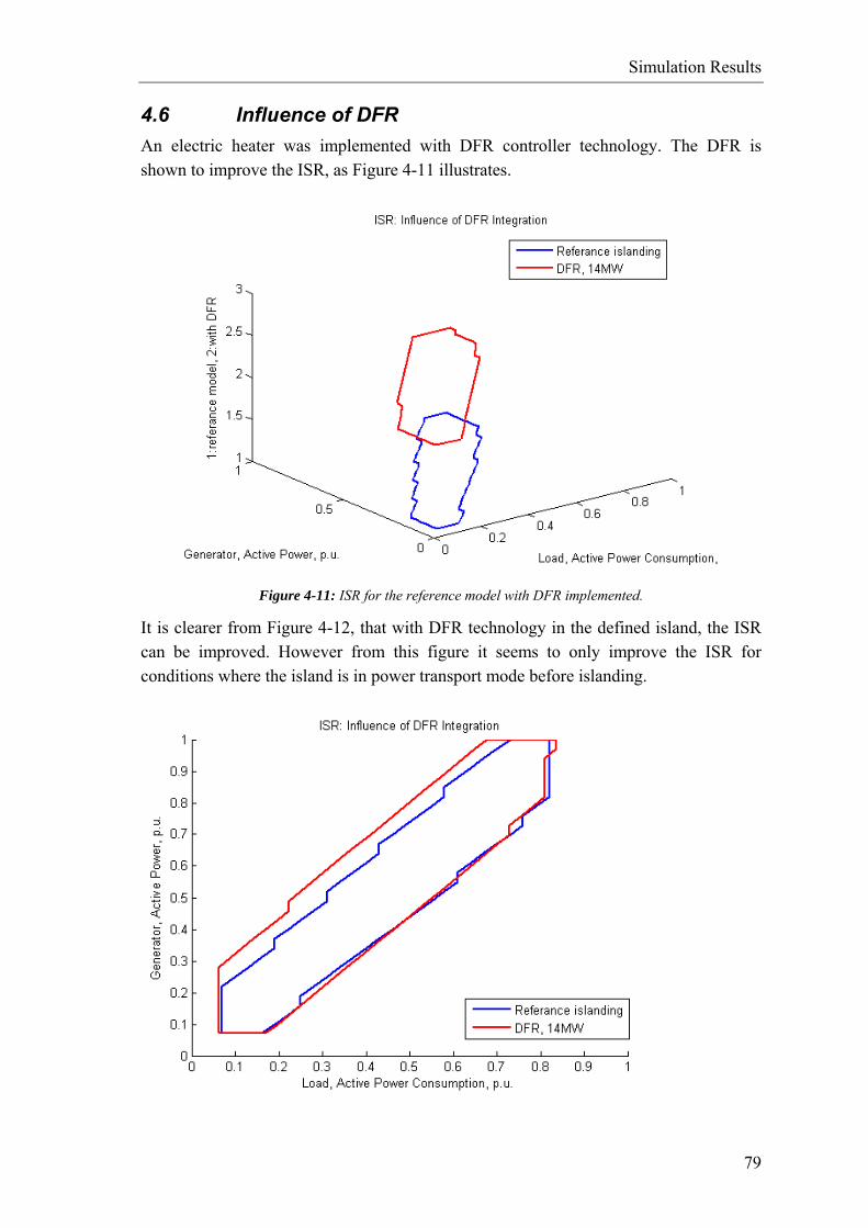
Simulation Results

79

4.6 Influence of DFR An electric heater was implemented with DFR controller technology. The DFR is shown to improve the ISR, as Figure 4-11 illustrates.

Figure 4-11: ISR for the reference model with DFR implemented.

It is clearer from Figure 4-12, that with DFR technology in the defined island, the ISR can be improved. However from this figure it seems to only improve the ISR for conditions where the island is in power transport mode before islanding.

Simulation Results

80

Figure 4-12: ISR for the reference model with DFR implemented.

4.7 Different Combination of Conventional Generators In this chapter the influence of different generator combination is tried. The results in Figure 4-13, shows that it does not have much impact on the general area of the ISR. Table 4-3 show the parameters used for this simulation. Parameter Value Unit Min generation 0,10 pu Max generation 0,90 pu Generation increments 0,03 pu Min load 0,10 pu Max load 0,90 pu Load increments 0.03 pu

Table 4-3: Simulation parameters for different combination of conventional generators.

The range simulated is reduced so that the generators are not in negative production, and that they are not overloaded before islanding transition.

Simulation Results

81

Figure 4-13: Different combinations of Conventional Generators.

The same results better illustrated, as shown from top in Figure 4-14.

Figure 4-14: Different combinations of Conventional Generators.

Simulation Results

82

The ISR is nearly unaffected of the different combinations. Only where the grid is highly loaded, is there a little difference in ISR. This can be partly explained by the fact that the machines in the reference island model are fairly similar.

4.8 Load Shedding By implementing frequency relays, the ISR can be improved as shown in Figure 4-15 and Figure 4-16. The ISR is improved as some of the loads are dropped when the island is being overloaded and the frequency becomes too low. The degree of improvement of the ISR depends on the amount of load shedding available.

Simulation Results

83

Figure 4-15: ISR for the reference model with two different load shedding implimentations.

Figure 4-16: ISR for the reference model with two different load shedding implimentations.

Simulation Results

84

From Figure 4-16, it is clear that the load shedding mostly improves the ISR for conditions when the defined island is in import mode before the islanding transition. This is because it will introduce under-frequency within the island after islanding transition. However in cases of overfrequencies, the load shedding offers little or no improvement.

4.9 Part Conclusion The different parameters for the generator, controller and prime mover were successfully simulater. The simulation results show tha ISR curve, where it can be compared to the reference model results as well as other results. The simulations results confirm the theoretical analysis on the influences of these different parameters. It is also found by simulations that both DFR and load shedding can improve the ISR region. And a combination of both technologies would potentially improve ISR further.

85

5 CONCLUSION

This project has investigated the influence of different generation types on the ISR. Also the impact of load shedding and the emerging energy technology DFR are investigated. The Islanding Security Region (ISR) used together with a control mechanism can potentially improve the reliability of the electric supply to customers. Simulation results and evaluation show that increased generator inertia can improve the ISR. This was clearly illustrated as the results for a reference island are compared to that of a reference island with increased generator inertia on the one hand and decreased inertia on the other. The turbine time constant, which should indicate how fast a turbine and its fuel system will react to controller input, showed that faster or slower time constant do not have a very big influence on the ISR unless the changes in the time constant are much greater compared to that of the reference model. The droop controller does influence the ISR and can improve the ISR area greatly, less droop gives better ISR. The generators in the reference model have a very low droop setting and lowering it further will not necessarily improve the ISR, as other factors will start to be decisive. Load shedding by frequency relays does show improvements to the ISR, and depending on the level of acceptable load shedding, the ISR can be improved considerably. However it should be noted that it only improves the lower region of the ISR curve, when the island is importing electric power at the time of islanding. Also the DFR can improve the ISR as shown with simulations. The investigation of different generation types on the ISR must be considered a very broad problem, as there are many aspects to consider. In this project most of the tasks on the tasklist are discussed and evaluated in the report. It is clear that most of the subjects handled in this project could be investigated in much more detail, for example it would be interesting to focus on different types power control in more detail. Some simplifications are justified with respect to influence of different generation types, so that the influence is primarily investigated by the means of varying the characteristic parameters of a generator, prime mover and controller unit.

Conclusion

86

Most of the work is done on adjusting and improvements to the program script for evaluating the ISR of a grid model. The improvements to the script allow for visual comparison of the influence for various generation types, as well as easier means of analyzing the simulation data. Even though there is an primarily focus on one type of an island model (Reference Island), the script could easily be adapted to any other grid model for quickly evaluating the ISR and influence of different generation types on that model. The plots shown in this report have a rather low resolution, and in some cases that makes comparing the different generation types difficult. The reason for not having higher resolution is to limit the simulation time, as simulations presented in this report take anything from 3 hours to 30 hours to execute. The program code and functions created for this project could be applied on other island models and other possibly more specific analysis.

87

REFERENCES

[1] Zhao Xu, Jacob Østergaard Yu Chen, "Control Mechanism and Security Region for intentional Islanding Transition," Article.

[2] Yu Chen, NextGen - Control Architecture for Inetntional Islanding Operation in Future Distribution Network with High Penetration of Distributed Generation, 2007-04-01 to 2010-03-31, Ongoing.

[3] Prabha Kundur, "Power System Stability and Control," in Power System Stability and Control, 1st ed.: McGraw-Hill, Inc., 1994, p. page 7.

[4] International Energy Agency. (2007, January) renewable_factsheet. [Online]. http://www.iea.org/papers/2006/renewable_factsheet.pdf

[5] Prabha Kundur, "Power System Stability and Control," in Power System Stability and Control.: McGraw-Hill, Inc., 1994, pp. 3 - 14.

[6] IEEE, "IEEE P1547.4/Draft 6.0 Draft Guide for Design, Operation and Integration of Distributed Resource Island Systems with Electric Power Systems," in Power System Stability and Control., 2009, pp. 13 - 17.

[7] IEEE, "IEEE P1547.4/Draft 6.0 Draft Guide for Design, Operation and Integration of Distributed Resource Island Systems with Electric Power Systems," IEEE, Guide, (draft) 2009.

[8] Prabha Kundur,.: Power System Stability and ControlMcGraw-Hill, Inc., 1994, pp. 17 - 45.

[9] Prabha Kundur,.: McGraw-Hill, Inc., 1994, p. 590. [10

] Norway, Sweden & Finland TSO’s of Denmark, "Nordic Grid Code 2007," in Nordic Grid Code 2007., 2007, p. 74.

[11]

Prabha Kundur, "Power System Stability and Control," in Power System Stability and Control.: McGraw-Hill, Inc., 1994, p. 128.

[12]

Mikael and Jacob Zhao, Demand as Frequency Controlled Reserve., 2008.

[13]

Mikael and Jacob Zhao, "Demand as Frequency Controlled Reserve," in Demand as Frequency Controlled Reserve., 2008, p. 18.

[14]

Mikael and Jacob Zhao, "Demand as Frequency Controlled Reserve," in Demand as Frequency Controlled Reserve., 2008, pp. page 33 - table 4.

Conclusion

88

[15]

Mikael and Jacob Zhao, "Demand as Frequency Controlled Reserve," in Demand as Frequency Controlled Reserve., 2008, p. 44.

[16]

Powercor Citipower. http://www.powercor.com.au. [Online]. http://www.powercor.com.au/docs/pdf/Customer%20Information/Fact%20Sheet%20-%20Load%20Shedding.pdf

[17]

DIgSILENT Power Factory, User Manual, 1322007th ed.

89

A MATLAB ISR SOURCE CODE AND FUNCTIONS

The following is a list of scripts and function created in matlab during the progress of this project. Despcrition of the scripts and functions is given within the files.

• evaluateISR.m • freqdev.m • freqtime.m • maxdfdt.m • outlineMatirx.m • outlineMatrix3D.m • paraChangeCounter.m • peakfreq.m • plot3DISR.m • plotISR.m • plotISR2d.m • plotOutlines.m • plotOutlines3D.m • plotSimple.m • read_txt.m • returnIndexed.m • sortMatrix.m • volttime.m

evaluateISR.m % script evaluateISR.m % % Purpose: Evaluate and plot ISR for PF simulation. % % Input: Simulation data files are input, and should be placed in % C:/matlab7/work, % file names should be % settings: settings2Txt.txt % conditions: case2Txt.txt % Freq and time arrays: freq2Txt.txt % voltage: volt2Txt.txt % Alternatively, the file locations could be added to matlab path % % Output: Plots of the ISR %

Matlab ISR Source code and functions

90

% written 2009 as a part of MSc thesis % Kristjan P Petursson, stnr. s071538 %Load data R=0; clc disp('Options:') disp(' Press "1" to use previously loaded data.') disp(' Press "2" to load Power Factory data.') disp(' Press "3" to cancel.') R=input('Press 1, 2 or 3:'); if R ==1 [N,M]=size(a); if N==0 disp('No data available. PF data will be loaded.') R=2; end disp('New data not loaded, previously loaded data will be used.') end if R==2 disp('Reading data...') clear a0=read_txt('settings2Txt.txt'); %setngs2Txt.txt is produced in pf disp('settings2Txt.txt is loaded') a=read_txt('freq2Txt.txt'); %freq_kpp.txt is produced in pf disp('freq2Txt.txt is loaded') a1=read_txt('volt2Txt.txt'); %volt_kpp.txt is produced in pf disp('volt_kpp.txt is loaded') aX=read_txt('case2Txt.txt'); %case_kpp.txt is produced in pf a2(1,:)=aX(1,:); %a2 holds only pu values of gen and load a2(2,:)=aX(2,:); a3(1,:)=aX(3,:); %a3 holds only anctual values of gen and load a3(2,:)=aX(4,:); [N,M]=size(aX); if N==5 a4(1,:)=aX(5,:); %holds any third varialbe that is beeing sweeped in simulation else disp('cases file has the following number of variables') disp(N) end clear aX; %clears the variable a4, as it is not used anymore. disp('case_kpp.txt is loaded') disp('Reading data completed.') elseif R==3 error('Operation aborted') end %characteristics and limits %limits for frequency %times where freq should be observed tBefore = 15; % to check freq before islanding tIsland = 20; % time when grid goes to island mode (external disconnected) tAfter = 15+1; % frequency should be within limits within 15 sec from dist. %Limits: %frequency limits fMinBefore=49.99; %freq limit before islanding fMaxBefore=50.01; %freq limit before islanding fMinAfter=49.8; %freq limit after islanding fMaxAfter=50.2; %freq limit after islanding dfdtMaxLim=2.5; %derivative freq limit %voltage limits vMinBefore=0.5; %freq limit before islanding vMaxBefore=1.5; %freq limit before islanding vMinAfter=0.8; %freq limit after islanding vMaxAfter=1.2; %freq limit after islanding

Matlab ISR Source code and functions

91

[N,M]=size(a); stableIndex=[]; %clearing stable indexes before starting sweep unstableIndex=[]; %clearing unst. indexes before starting sweep nrStable=0; %clearing number of stable cases nrUnstable=0; %clearing number of unstable cases allCases=[]; allStableCases=[]; allUnstableCases=[]; %sort data, freq, volt, P and Load into matrixes k=1; %is counter for the loop and indexes where %we are in the freq matrix. k1=1; %is counter for the loop and indexes where %we are in the volt matrix. while k<=M b=[]; %resets the matrixes bb=[]; d=[]; h=1; while h<=N if a(h,k)~= 0 %stoppes filling b&c when values are zero. b(h,1)=a(h,k); %b array holds frequency values, while... bb(h,1)=a(h,k+1); %c array holds the time values, while... end h=h+1; end h=1;%loop for creating volt arrays if k1<=M/2 while h<=N if a1(h,k1)~= 0 %stoppes filling when values are zero. d(h,1)=a1(h,k1); %d array holds volt values. end h=h+1; end end %---------------------------------------------------------------------- %get freq data before and after islanding fBefore=volttime(b,bb,tBefore); %freq before islanding vBefore=freqtime(d,bb,tBefore); %voltage before islanding fAfter=freqtime(b,bb,tIsland+tAfter); %freq after islanding vAfter=volttime(d,bb,tIsland+tAfter); %volt after islanding [fDevMin,fDevMax]=freqdev(b); %check freq deviation dfdtMax=maxdfdt(b,bb); %check freq derivative %function uses absolute value, so there %is no need for min. %check if stable stable=0; %variable stable is assumed 0(unstable) %untill check reveals 1(stable) allCases(1,k1)=fBefore; allCases(2,k1)=fAfter; allCases(3,k1)=dfdtMax; allCases(4,k1)=vBefore; allCases(5,k1)=vAfter; %this criteria checks only if freq is within limits before and %after islanding, no voltage or derivative criteria

Matlab ISR Source code and functions

92

%Consider freq before Island, after island and derivative during %whole simulation %Consider freq and voltage before and after, derivative not included if fBefore<=fMaxBefore && fBefore>=fMinBefore... %freq crit && fAfter<=fMaxAfter && fAfter>=fMinAfter... %freq crit && vBefore<vMaxBefore && vBefore>vMinBefore... %volt crit && vAfter<vMaxAfter && vAfter>vMinAfter %volt crit % % %Consider only freq criterion % if fBefore<=fMaxBefore && fBefore>=fMinBefore... %freq crit % && fAfter<=fMaxAfter && fAfter>=fMinAfter... %freq crit % % %Consider df/dt criterion % if fBefore<=dfdtMax <= dfdtMaxLim... %derivative % % %Consider only voltage criterion % if fBefore<= vBefore<vMaxBefore && vBefore>vMinBefore...%volt crit % && vAfter<vMaxAfter && vAfter>vMinAfter %volt crit stable=1; %marking simulation instance as stable end %actions to be taken when stable case is found can be added under %the following "if" if stable == 1 nrStable=nrStable+1; %Save stable indexis %note "(k+1)/2" will index the right column in the case %matrix (a2). stableIndex(nrStable,1)=(k+1)/2; allStableCases(1,nrStable)=fBefore; allStableCases(2,nrStable)=fAfter; allStableCases(3,nrStable)=dfdtMax; allStableCases(4,nrStable)=vBefore; allStableCases(5,nrStable)=vAfter; else nrUnstable=nrUnstable+1; %Save unstablestable indexis %note "(k+1)/2" will index the right column in the case %matrix (a2). unstableIndex(nrUnstable,1)=(k+1)/2; allUnstableCases(1,nrUnstable)=fBefore; allUnstableCases(2,nrUnstable)=fAfter; allUnstableCases(3,nrUnstable)=dfdtMax; allUnstableCases(4,nrUnstable)=vBefore; allUnstableCases(5,nrUnstable)=vAfter; end k1=k1+1; k=k+2; %----------------------------------------------------------------- end %------------------------------------ %now Stable cases have been found and indexed, ISR region can therefore be %plotted: %if there are made Powerfactory simulations where the third parameter is %beeing, sweeped, that is not only load and generation, the results will be %sorted so that the results can be displayed correctly. %check if simulations have been set to 3D (done in PF ISR script) if a0(1,1)==1 %then the plot has the third parameter. a2stable= returnIndexed(a2,stableIndex); a3stable= returnIndexed(a3,stableIndex); a4stable= returnIndexed(a4,stableIndex); %full plot with X marking stable cases, O is unstable figure clf %clears old graphics from figure figurenr=gcf; %gets number of created figure

Matlab ISR Source code and functions

93

set(figurenr,'color',[1 1 1]) hold on if nrStable ~=0 %so if nr stable is zero, then nothing to plot plotISR([a2;a4],stableIndex,'x') end if nrUnstable ~=0 %so if nrunstable is zero, then nothing to plot plotISR([a2;a4],unstableIndex,'ro') end title('ISR region 3D') ylabel('Generator, Real Power Production') xlabel('Load, Real Power Consumption') zlabel('3rd parameter') axis auto view(3) hold off %plot 3d outlines plot3DISR([a2stable;a4stable]) elseif a0(1,1)==0 %then its normal 2d plot %plot with pu values figure clf %clears old graphics from figure figurenr=gcf; %gets number of created figure set(figurenr,'color',[1 1 1]) hold on plotISR2D(a2,stableIndex,'x') %plots stable cases plotISR2D(a2,unstableIndex,'ro') %plots unstable cases title('ISR region') ylabel('Generator, Active Power, p.u.') xlabel('Load, Active Power Consumption, p.u.') axis([0.1 1.0 0.1 1.]) view(2) hold off %plot with actual values figure clf %clears old graphics from figure figurenr=gcf; %gets number of created figure set(figurenr,'color',[1 1 1]) hold on plotISR2D(a3,stableIndex,'x') %plots stable cases plotISR2D(a3,unstableIndex,'ro') %plots unstable cases title('ISR region') ylabel('Generator, Active Power, [MW]') xlabel('Load, Active Power Consumption, [MW]') axis([0.1*272 1.0*272 0.1*272 1*272]) view(2) hold off %make outlineplot of region %create outline matrix for pu plot a2stable= returnIndexed(a2,stableIndex); ISRoutlines=outlineMatrix(a2stable); %plot outlines figure(1) hold on plotOutlines(ISRoutlines) hold off %create outline matrix for actual values plot a3stable= returnIndexed(a3,stableIndex); ISRoutlines=outlineMatrix(a3stable); %plot outlines figure(2) hold on plotOutlines(ISRoutlines) hold off end

Matlab ISR Source code and functions

94

%--------------------------------------

Freqdev.m function [min,max]=freqdev(freq) % % Purpose: finds the deviation, given that its a 50Hz system, max and min % % Input: freq is a vector of the frequency values. % % Output: max returns the double value for the positive peak frequency % deviation % min returns the double value for the negatative(or lowest) peak % frequency deviation % % written 2009 as a part of MSc thesis % Kristjan P Petursson, stnr. s071538 [N,M]=size(freq); k=1; max=0; %assuming 50Hz system, the start values for max and min will min=0; %... as shown here, 50Hz while k<=N f1=freq(k,1)-50; %-50 because it is a 50Hz system if f1>max max=f1; end if f1<min min=f1; end k=k+1; end %alternatively, could have used functions max & min return

• freqtime.m function freqt=freqtime(freq,time,t1) % % Purpose: gets frequency at chosen time in the simulation % % Input: freq is a vector of the frequency values. % time is a vector of the time values % t1 is a double value for the time of interest, where freq will % be extracted % % Output: freqt is the frequency at the chosen time % % written 2009 as a part of MSc thesis % Kristjan P Petursson, stnr. s071538 [N,M]=size(freq); k=0; t2=0; while t2<=t1 k=k+1; t2=time(k,1); end freqt=freq(k,1); return

• maxdfdt.m

Matlab ISR Source code and functions

95

function max=maxdfdt(freq,time) % % Purpose: finds the highest derivative for the frequency to be analysed % % Input: freq is a vector of the frequency values. % time should be the time vector supplied with the frequency % % Output: max returns the double value for the highest derivative of the % supplied freq,time % % written 2009 as a part of MSc thesis % Kristjan P Petursson, stnr. s071538 [N,M]=size(freq); k=2; max=0; while k<=N && freq(k,1)> 5 f1=freq(k-1,1); f2=freq(k,1); t1=time(k-1,1); t2=time(k,1); %calculate the df/dt df=abs(f2-f1); dt=abs(t2-t1); if dt ~=0 dfdt=df/dt; if dfdt>max max=dfdt; end end k=k+1; end return

• outlineMatirx.m function outMatrix=outlineMatrix(cases) % % Purpose:Creates outlines of the ISR region % % Input: cases is the gen and load settings for each simulation % index, indexes which ones of the cases are stable % % Output: OUT is a x,y matrix of the outlines of the ISR region % % written 2009 as a part of MSc thesis % Kristjan P Petursson, stnr. s071538 [N,M]=size(cases); k=1; k2=1; while k<=M %get data if cases(1,k)~= 0 YX(k2,1)=cases(1,k); %gen YX(k2,2)=cases(2,k); %load k2=k2+1; end k=k+1;

Matlab ISR Source code and functions

96

end %the Gen part is always growing, while load goes in loops, therefore we %know gen starts at its lowest value and goes upwards. %first point will be bottom left (min gen, min load) Gen=YX(1,1); [N,M]=size(YX); k=1; p=1; k1=1; while k <= N if YX(k,1)==Gen temp(k1,1)=YX(k,2); %saves the load value for each gen setting into an array %needs another counter that starts from 1 %in each loop else maxTemp(p,:)=[Gen,max(temp)]; minTemp(p,:)=[Gen,min(temp)]; temp=[]; %resets temp and counter for varialble k1=0; Gen=YX(k,1); k=k-1; %needs to go down here to counteract +1 below p=p+1; %because one point was found end if k==N %final loop to get the higest gen value maxTemp(p,:)=[Gen,max(temp)]; minTemp(p,:)=[Gen,min(temp)]; Gen=YX(k,1); end k=k+1; k1=k1+1; end %now to make it plot-able, they must be sorted: [N,M]=size(maxTemp); p_counter=1; p_counter2=1; while p_counter<=N outMatrix(p_counter2,:)=maxTemp(p_counter,:); p_counter=p_counter+1; p_counter2=p_counter2+1; end p_counter=p_counter-1; while p_counter>0 outMatrix(p_counter2,:)=minTemp(p_counter,:); p_counter=p_counter-1; p_counter2=p_counter2+1; end %the last point must be added to be the same as first to finish closed area [N,M]=size(outMatrix); outMatrix(N+1,:)=outMatrix(1,:);

Matlab ISR Source code and functions

97

• outlineMatrix3D.m function outMatrix=outlineMatrix3D(cases) % % Purpose:Creates outlines of the ISR region % % Input: cases is the gen and load settings for each simulation % index, indexes which ones of the cases are stable % % Output: OUT is a x,y matrix of the outlines of the ISR region % % written 2009 as a part of MSc thesis % Kristjan P Petursson, stnr. s071538 ZZ=cases(3,1); %inertia is not changin in this function, stored in ZZ [N,M]=size(cases); k=1; k2=1; while k<=M %get data if cases(1,k)~= 0 YX(k2,1)=cases(1,k); %gen YX(k2,2)=cases(2,k); %load k2=k2+1; end k=k+1; end %the Gen part is always growing, while load goes in loops, therefore we %know gen starts at its lowest value and goes upwards. %first point will be bottom left (min gen, min load) Gen=YX(1,1); [N,M]=size(YX); k=1; p=1; k1=1; while k <= N if YX(k,1)==Gen temp(k1,1)=YX(k,2); %saves the load value for each gen setting into an array %needs another counter that starts from 1 %in each loop else maxTemp(p,:)=[Gen,max(temp),ZZ]; minTemp(p,:)=[Gen,min(temp),ZZ]; temp=[]; %resets temp and counter for varialble k1=0; Gen=YX(k,1); k=k-1; %needs to go down here to counteract +1 below p=p+1; %because one point was found end if k==N %final loop to get the higest gen value maxTemp(p,:)=[Gen,max(temp),ZZ]; minTemp(p,:)=[Gen,min(temp),ZZ]; Gen=YX(k,1); end k=k+1; k1=k1+1; end

Matlab ISR Source code and functions

98

%now to make it plot-able, they must be sorted: [N,M]=size(maxTemp); p_counter=1; p_counter2=1; while p_counter<=N outMatrix(p_counter2,:)=maxTemp(p_counter,:); p_counter=p_counter+1; p_counter2=p_counter2+1; end p_counter=p_counter-1; while p_counter>0 outMatrix(p_counter2,:)=minTemp(p_counter,:); p_counter=p_counter-1; p_counter2=p_counter2+1; end %the last point must be added to be the same as first to finish closed area [N,M]=size(outMatrix); outMatrix(N+1,:)=outMatrix(1,:);

• paraChangeCounter.m

function sortedMatrix=paraChangeCounter(cases) % % Purpose: sort cases by the value of the third parameter, this helps with % plotting the ISR % % Input: matrix of parameter values % % Output: matrix returns how often it changed % % written 2009 as a part of MSc thesis % Kristjan P Petursson, stnr. s071538 [N,M]=size(cases); k=1; k2=1; temp=cases(3,1); %just putting some value that will not befound... counter=1; % in any parameters while k<=M sortedMatrix(k2,counter)=cases(k,1); sortedMatrix(k2,counter+1)=cases(k,2); sortedMatrix(k2,counter+2)=cases(k,3); if cases(3,k)~=temp temp=cases(1,k); counter=counter+3; k2=0; %reset this counter because need too %start in new line in sorted matrix end k2=k2+1; k=k+1; end

• peakfreq.m

function [min,max]=peakfreq(freq) % % Purpose: finds the peak frequencies, max and min % % Input: freq is a vector of the frequency values. % % Output: max returns the double value for the positive peak frequency % min returns the double value for the negatative(or lowest) peak frequency %

Matlab ISR Source code and functions

99

% written 2009 as a part of MSc thesis % Kristjan P Petursson, stnr. s071538 [N,M]=size(freq); k=1; max=50; %assuming 50Hz system, the start values for max and min will min=50; %... as shown here, 50Hz while k<=N f1=freq(k,1); if f1>max max=f1; end if f1<min min=f1; end k=k+1; end %alternatively, could have used functions max & min return

• plot3DISR.m

function plot3DISR(cases) % % Purpose:Takes care of data for 3d plotting and plots % % Input: cases is the stable gen, load and 3rd parameter matrix % % Output: plot of ISR region in 3d % % written 2009 as a part of MSc thesis % Kristjan P Petursson, stnr. s071538 %plot outlines of each most outer loop, making a 3D plot sortedCases=sortMatrix(cases); [N,M]=size(sortedCases); k=1; figure hold on while k <= N ISRoutlines=outlineMatrix3D([sortedCases(k,:);sortedCases(k+1,:);sortedCases(k+2,:)]); plotOutlines3D(ISRoutlines) k=k+3; end hold off

• plotISR.m

function plotISR(cases,index,color) % % Purpose:plots 3d of the ISR region, gen, load and a third variable(f.x. % inertia) % % Input: cases is the gen and load settings for each simulation % index, indexes which ones of the cases are stable % % Output: plot of stable region % % written 2009 as a part of MSc thesis % Kristjan P Petursson, stnr. s071538 %figure figurenr=gcf; %gets number of created figure

Matlab ISR Source code and functions

100

set(figurenr,'color',[1 1 1]) hold on [N,M]=size(index); k=1; while k<=N %get index ind=index(k,1); %get3d data y=cases(1,ind); x=cases(2,ind); z=cases(3,ind); %mark on plot where system is stable plot3(x,y,z,color); k=k+1; end hold off

• plotISR2d.m

function plotISR2D(cases,index,color) % % Purpose:plots 2d of the ISR region, only of gen and load are the only % variables % % Input: cases is the gen and load settings for each simulation % index, indexes which ones of the cases are stable % color should be a string, indicating what color to plot and symbol % % Output: plot of stable region % % written 2009 as a part of MSc thesis % Kristjan P Petursson, stnr. s071538 [N,M]=size(index); if N<1 disp('function plotISR2D(cases,index): to few stable cases') return end k=1; while k<=N %get index ind=index(k,1); %get3d data y=cases(1,ind); %gen x=cases(2,ind); %load %mark on plot where system is stable plot(x,y,color); k=k+1; end

• plotOutlines.m

Matlab ISR Source code and functions

101

function plotOutlines(outLineMatrix) % % Purpose: plots outlines of the ISR % % Input: outLineMatrix is the outline matrix, holding the outline points % % Output: plots of the ISR. % % written 2009 as a part of MSc thesis % Kristjan P Petursson, stnr. s071538 if outLineMatrix ==1 disp('function plotOutlines(outLineMatrix): Nothing to plot') return end X=outLineMatrix(:,1); Y=outLineMatrix(:,2); plot(Y,X,'k','LineWidth',2)

• plotOutlines3D.m

function plotOutlines3D(outLineMatrix) % % Purpose: plots outlines of the ISR in 3 dimension, including the third % parameter sweep (not only load and generation) % % Input: outLineMatrix is the outline matrix, holding the outline points % % Output: plots of the ISR 3d. % % written 2009 as a part of MSc thesis % Kristjan P Petursson, stnr. s071538 if outLineMatrix ==1 disp('function plotOutlines(outLineMatrix): Nothing to plot') return end size(outLineMatrix) X=outLineMatrix(:,1); Y=outLineMatrix(:,2); Z=outLineMatrix(:,3); plot3(Y,X,Z)

• plotSimple.m function plotSimple(cases,casenr) % % Purpose:plots the freq over time % % Input: cases is all the f vectors % casenr is the number of which one to plot % % Output: plot of frequency for chosen case. % % written 2009 as a part of MSc thesis % Kristjan P Petursson, stnr. s071538 [N,M]=size(cases); casenr=casenr*2; b=[]; %resets the matrixes c=[];

Matlab ISR Source code and functions

102

h=1; while h<=N && cases(h,casenr-1)>5 %stoppes filling b&c when values are zero. b(h,1)=cases(h,casenr-1); %b array holds frequency, while... c(h,1)=cases(h,casenr); %c array holds the time. h=h+1; end plot(c,b)

• read_txt.m

function b=read_txt(filename); % % Purpose: reads a costum made Powerfactory variable file in txt format % (Variables saved in columns). % % Input: filename should be a string, the name of the file to load % % Output: b returns the double value matrix with the information stored in % the txt file % % written 2009 as a part of MSc thesis % Kristjan P Petursson, stnr. s071538 fid = fopen(filename); c=0; %var only used as counter while 1 c= c+1; tline = fgetl(fid); %disp(tline) if ~ischar(tline), break, end if tline ~= -1 %this is to skip final string in tline which is -1 a=str2num(tline); if size(a)~=[0,0] % to abvoid filling the first row with blanks %disp(a) b(c,:)=a; else end else end end fclose(fid); return

• returnIndexed.m function x=returnIndexed(data,index) % % Purpose: Returns the indexed columns from the matrix/array called data % % Input: data is a vector or matrix % index should index the columns that will be returned

Matlab ISR Source code and functions

103

% % Output: x is the resulting matrix % % written 2009 as a part of MSc thesis % Kristjan P Petursson, stnr. s071538 [N,M]=size(index); [N,M]=size(index); if N<1 disp('function returnIndexed(data,index): to few stable cases') x=1; return end k=1; while k<=N k2=index(k,1); %gets the reference from the index matrix x(:,k)=data(:,k2); %gets the indexed value from data matrix k=k+1; end

• sortMatrix.m function sortedMatrix=sortMatrix(cases) % % Purpose: sort cases by the value of the third parameter, this helps with % plotting the ISR % % Input: matrix of stable parameter values, Gen, Load and third parameter % % Output: matrix returns how often it changed % % written 2009 as a part of MSc thesis % Kristjan P Petursson, stnr. s071538 [N,M]=size(cases); k=1; k2=1; temp=cases(3,1); %just putting some value that will not befound... counter=1; % in any parameters counter2=1; while k<=M %identify change in 3rd parameter, if it changes, counters are set %abd temp value for comparison is updated. if cases(3,k)~=temp temp=cases(3,k); counter=counter+3; counter2=counter2+1; %returns the number of changes in param k2=1; %reset this counter because need too %start in new line in sorted matrix end sortedMatrix(counter,k2)=cases(1,k); sortedMatrix(counter+1,k2)=cases(2,k); sortedMatrix(counter+2,k2)=cases(3,k); k2=k2+1; k=k+1; end

Matlab ISR Source code and functions

104

• volttime.m

function voltt=volttime(volt,time,t1) % % Purpose: gets voltage at chosen time in the simulation % % Input: volt is a vector of the voltage values. % time is a vector of the time values % t1 is a double value for the time of interest, where volt will % be extracted % % Output: voltt is the voltage at the chosen time (t1) % % written 2009 as a part of MSc thesis % Kristjan P Petursson, stnr. s071538 [N,M]=size(volt); k=0; t2=0; while t2<=t1 k=k+1; t2=time(k,1); end voltt=volt(k,1); return

105

B POWER FACTORY ISR SOURCE CODE

The following is the variables introduced in the basic options window: Type Var name value description int 3D 1 tells matlab if it should make 3d plots or 2d double ScaleLoad 0.03 Scale for Loads double ScaleGen 0.03 Scale for Gens double Pgenmaxpct 0.90 Percentage of base gen‐max double Pgenminpct 0.10 Percentage of base gen‐min double Ploadmaxpct 0.90 Percentage of base load‐max double Ploadminpct 0.10 Percentage of base load‐min double Tstop 40 s Stop time, or total simulation time double Tstart ‐0.01 s Start time double Tstep 0.01 s Step time double Tisland 20 s Islanding moment

double Tobserve 15 sFreq. observed time moment for assessment, after islanding

double Tbefore 10 s Freq0, acquired at the time before islanding string Busisland 'Bus 8' the bus for frequency observation in island string Busexternal 'Bus 1' the bus for frequency observation in external grid

string path route/path for output window files. (with *.out extension file name)

string freqTxt 'C:\MATLAB7\work\freq2Txt.txt' Path to frequency and time result file string caseTxt 'C:\MATLAB7\work\case2Txt.txt' Path to case result file string voltTxt 'C:\MATLAB7\work\volt2Txt.txt' Path to Voltage result file

string settingsTxt 'C:\MATLAB7\work\settings2Txt.txt' Path to settings (to determine how to handle result files in matlab)

double maxDiff 80 max abs diff of load &gen, or sim is skipped (saves time) double xtramaxpct 15 This will be used as a max for third paramter double xtraminpct 5 This will be used as a min for third paramter double xtraStep 5 This will be used as a stepsize for third paramter

The following is the source code of the ISR script part from PF. ** the code is from [1] but modified for the purpose of this project. !------------------------------! !Internal Variables definitions! !------------------------------! int selected;!used for reminding operator of 'General Selection'. int l, g; !used for counting how many Loads and Gens.

Power Factory ISR Source Code

106

int i;!used for incease of Load scale int j;!used for incease of Gen scale int k; int z, zz; int Nval, Nvar; int Nfreq, Nfreq0; !used to identify the 'Nfreq'th frequency we want int i1; !i1 represents the number of varialbe 'm:fehz' int i5; !is the voltage m:u int h; int m; int pNRow, r, rr, rrr; int a, b, c, d, aa, bb; int dd; !XXXX kpp addition int kp1, kp2, kp3,kp4, ticktack; double kpp1,NvalMax,corrFactor,Pgenratetot2,xtraVal,ticktackvar; !xxxxx double Ploadmax, Ploadmin, Pgenmax, Pgenmin; double Pgentot, Pgentot1, Ploadtot, Ploadratetot, Pgenratetot;!total Power of Gens and Loads double pplini; double x, y;!used to calculate how many circles for load double Scaleloadmin, Scaleloadmax, Scalegenmin, Scalegenmax; double Pgenrate1, Pgenrate2, Pgenrate3, Pgenrate4, Pgenrate5; double Pgen1, Pgen2, Pgen3, Pgen4, Pgen5; double time, freq, freq0, freqresA, freqresB, loadresA, loadresB, loadres0; double mi, nj; double valueMatrix; double valueMatrixStable; double normal, min, max; double v1, v2; double minimum, maximum, GenPower; double P; double cc, cc1, cc2, loadmintop, loadmaxtop, loadmindown, loadmaxdown, pgenmax, pgenmin; double value; object pComInc, pComSim, ObejctInRes;!used for getting Commands. object O; object pEvent, pSwitchEvt; object switchevent; object res; object aGrf, aPg, aPg1, aPlot1, aPlot2, aPlot3, aPlot4; object bus1, bus2; object OO; object case; object Redirect; string generator; set sAllLoad, sAllGen;!used for collecting all loads and Gens. set allElements; !holds all elements set Events; set Pload, Pgen; set allbus; !----------------! !Program starting! !----------------! ClearOutput(); EchoOff(); NvalMax=0; MatrixRes.Init(1,6); MatrixRes.ColLbl('freqresA', 1); MatrixRes.ColLbl('loadresA', 2); MatrixRes.ColLbl('freqresB', 3); MatrixRes.ColLbl('loadresB', 4); MatrixRes.ColLbl('loadres0', 5); MatrixRes.ColLbl('Pgentot', 6);

Power Factory ISR Source Code

107

Matrixall.Init(1,4); Matrixall.ColLbl('freqres', 1); Matrixall.ColLbl('loadres', 2); Matrixall.ColLbl('loadres0', 3); Matrixall.ColLbl('Pgentot', 4); MatrixStable.Init(1,4); MatrixStable.ColLbl('freqres', 1); MatrixStable.ColLbl('loadres', 2); MatrixStable.ColLbl('loadres0', 3); MatrixStable.ColLbl('Pgentot', 4); MatrixMinMax.Init(1, 3); MatrixMinMax.ColLbl('MIN', 1); MatrixMinMax.ColLbl('MAX', 2); MatrixMinMax.ColLbl('Pgentot', 3); Max.Init(1, 2); Max.ColLbl('Max', 1); Max.ColLbl('Pgentot', 2); Min.Init(1, 2); Min.ColLbl('Min', 1); Min.ColLbl('Pgentot', 2); ParaLLEL.Init(1,2); ParaLLEL.ColLbl('load',2); ParaLLEL.ColLbl('Pgentot',2); MatrixCurve.Init(1,18); MatrixCurve.ColLbl('MINIMUM', 1); MatrixCurve.ColLbl('MAXIMUM', 2); MatrixCurve.ColLbl('TOTGEN', 3); MatrixCurve.ColLbl('Pmax', 4); MatrixCurve.ColLbl('Pmin', 5); MatrixCurve.ColLbl('Plodlimit', 6); MatrixCurve.ColLbl('Plodlimit1', 7); MatrixCurve.ColLbl('xaxis', 8); MatrixCurve.ColLbl('yaxis', 9); MatrixCurve.ColLbl('MINIMUMpct', 10); MatrixCurve.ColLbl('MAXIMUMpct', 11); MatrixCurve.ColLbl('TOTGENpct', 12); MatrixCurve.ColLbl('Pmaxpct', 13); MatrixCurve.ColLbl('Pminpct', 14); MatrixCurve.ColLbl('Plodlimitpct', 15); MatrixCurve.ColLbl('Plodlimit1pct', 16); MatrixCurve.ColLbl('xaxispct', 17); MatrixCurve.ColLbl('yaxispct', 18); MatrixXY.Init(1, 2); MatrixXY.ColLbl('X', 1); MatrixXY.ColLbl('Y', 2); !Internal Variables definitions !Results.Init(); !pComInc.p_resvar=Results; !pComInc.Execute(); !Remind operator if all grid has been selected as 'General Selection' on page 'Basic Options' input(selected, 'All in "General Selection"?(0-Yes, 1-No)'); if (selected=1) exit(); output('General Selection is ready.'); !Get Commands: 'Calculation of Initial Conditions'&'Run Simulation' !pComLdf=GetCaseObject('ComLdf'); pComInc=GetCaseObject('ComInc'); pComSim=GetCaseObject('ComSim'); !Execute commands: 'Calculation of Initial Conditions'&'Run Simulation' !pComSim.Execute(); !Get All loads and All Gens

Power Factory ISR Source Code

108

sAllLoad=SEL.AllLoads(); sAllGen=SEL.AllSym(); pComInc.Execute(); !Count how many loads and Gens l=sAllLoad.Count(); g=sAllGen.Count(); printf('There are \cc%d \caLoads and \cc%d \caGens.', l, g); printf('(including in service and out of service.)'); !output all loads' rates !!Sort objects in the set to their name from A to Z sAllLoad.SortToName(0); sAllGen.SortToName(0); !---------------- !Print all loads. !---------------- O=sAllLoad.First(); !Q=sAllLoadorigin.First(); !parameter 'outserv' represents 'out of service': !0 means in service, 1 means out of service. if (O) printf(' \ceLOAD NAME | \ccRATE MW'); !else !printf('\ccThere is no load.'); !exit(); !parameter 'outserv' represents 'out of service': 0 means in service, 1 means out of service Ploadtot=0;!indicate total power of loads. h=0; while (O) if (O:outserv=0) h+=1; printf('\ce%10s \cc%f',O:loc_name, O:plini); !printf('\ce%10s \cc%f',O:loc_name, O:m:P:bus1); !printf('%10s %f',O:loc_name, O:plini); Ploadtot=Ploadtot+O:plini; !Q:pplini=O:plini; O=sAllLoad.Next(); !Q=sAllLoadorigin.Next(); Ploadratetot=Ploadtot;!store the rated total power to 'Ploadratetot' if (h=0) printf('\ccThere is no loads.'); exit(); else printf('Total rated Load Power: \cc%f \caMW', Ploadratetot); printf('There are \cc%d \caLoads in service.', h); Ploadmax=Ploadratetot*Ploadmaxpct; Ploadmin=Ploadratetot*Ploadminpct; printf('----------------------------------------------'); printf('Ploadmax=\cc%f\caMW Ploadmin=\cc%f \caMW', Ploadmax, Ploadmin); printf('----------------------------------------------'); !----------------------------------------------------------- !Define Gen. Matrix, which stores rated power for every Gen. !----------------------------------------------------------- !freqMatrix.Init(1,1); !voltMatrix.Init(1,1); !caseMatrix.Init(1,1);

Power Factory ISR Source Code

109

MatrixGen.Init(1, 1); h=0; O=sAllGen.First(); while (O) if (O:outserv=0) h+=1; MatrixGen.Resize(1, h); MatrixGen.ColLbl(O:loc_name, h); MatrixGen.Set(1, h, O:P_max); O=sAllGen.Next(); if (h=0) printf('\ccThere is no Gen.'); exit(); !---------------------- !output all Gens' rates !---------------------- O=sAllGen.First(); if (O) printf(' \ceGEN NAME | \ccRATE MW'); !else !printf('\ccThere is no Gen.'); !exit(); m=1; Pgenratetot=0;!rated real power !Pgenratetot2=0;!is the rated real power while (m<=h) generator=MatrixGen.ColLbl(m); !valueMatrix=MatrixGen.Get(1, m); !dispatched valueMatrix=MatrixGen.Get(1, m); !rated power printf('\ce%10s | \cc%f', generator, valueMatrix); Pgenratetot=Pgenratetot+valueMatrix; !real dispatched power !Pgenratetot2=Pgenratetot2+valueMatrix2; !(real rated power) m+=1; !corrFactor= Pgenratetot/Pgenratetot2; !will be used to display actual rated power on plots(not dispatched) printf('Total Current Output Gens: \cc%f MW', Pgenratetot); printf('Total Rated Gens: \cc%f MW', Pgenratetot2); printf('There are \cc%d Gens:', h); printf('CurrentOutput/Ratedoutput = \cc%f :', corrFactor); Pgenmax=Pgenratetot*Pgenmaxpct; Pgenmin=Pgenratetot*Pgenminpct; printf('--------------------------------------------'); printf('Pgenmax=\cc%f MW Pgenmin=\cc%f MW', Pgenmax, Pgenmin); printf('--------------------------------------------'); !---------------------------------------------------- !----------------------------------------- !define simulation time and islanding time !----------------------------------------- pComSim:tstop=Tstop;!Stop time, or simulation time pComInc:tstart=Tstart;!Start time, can be negative !pComInc:dtout=Tstep;!Step time pComInc:dtgrd=Tstep;!Step time: pComInc:dtout above has no effect. printf('Simulation starts at \ceTstart=\cc%8.5f \cas', pComInc:tstart); printf('Time step is: \ceTstep=\cc%8.5f \cas', pComInc:dtout); printf('Simulation stops at \ceTstop=\cc%8.5f \cas', pComSim:tstop); !-------------------

Power Factory ISR Source Code

110

!Search Switch Event !------------------- pEvent=pComInc:p_event; Events=pEvent.GetContents(); pSwitchEvt=Events.FirstFilt('*.EvtSwitch'); !pSwitchEvt=Events.FirstFilt('island.EvtSwitch'); !if (pSwitchEvt.and.pSwitchEvt:outserv=0) !switchevent=pSwitchEvt; ! while(pSwitchEvt) if (pSwitchEvt:outserv=0) switchevent=pSwitchEvt; pSwitchEvt=Events.NextFilt(); !if (pSwitchEvt=0) !printf('There is no SwitchEvent.'); !exit(); ! switchevent:time=Tisland;!islanding time printf('Island moment at \ceTisland=\cc%f \cas', Tisland); ! !-------------------------------------- !Define change range for loads and Gen. !-------------------------------------- !how many cycles for load change? i=floor((1-Ploadminpct)/ScaleLoad)*(-1); mi=floor((Ploadmaxpct-1)/ScaleLoad); Scaleloadmin=1+ScaleLoad*i; Scaleloadmax=1+ScaleLoad*mi; !Scaleloadmax=1+ScaleLoad*floor((Ploadmax/Ploadratetot-1)/ScaleLoad); printf('Load changes from \cc%f \cato \cc%f, \caby ScaleLoad.', Scaleloadmin, Scaleloadmax); !how many cycles for Gen. change? j=floor((1-Pgenminpct)/ScaleGen)*(-1); nj=floor(((Pgenmax/Pgenratetot)-1)/ScaleGen); printf('j is \cc%f \ca and jn is \cc%f ', j, nj); !j=floor((1-Pgenmin/Pgenratetot)/ScaleGen)*(-1); Scalegenmin=1+ScaleGen*j; Scalegenmax=1+ScaleGen*nj; !Scalegenmax=1+ScaleGen*floor((Pgenmax/Pgenratetot-1)/ScaleGen); printf('Gen. changes from \cc%f \cato \cc%f, \caby ScaleGen.', Scalegenmin, Scalegenmax); !-------------------------------------------- !define variables to observe system frequency !-------------------------------------------- allbus=SEL.AllBars(); bus1=allbus.FirstFilt(Busisland); bus2=allbus.FirstFilt(Busexternal); NewIslandingResults.AddVars(bus1, 'm:fehz'); NewIslandingResults.AddVars(bus2, 'm:fehz'); NewIslandingResults.AddVars(bus1, 'm:u'); !pComInc:p_resvar=NewIslandingResults; !pComInc.Execute(); !pComSim.Execute(); !--------- !draw plot !--------- pComInc:p_resvar=NewIslandingResults; aGrf=GetGraphBoard();

Power Factory ISR Source Code

111

if (aGrf) aPg=aGrf.GetPage('Frequency', 1); if (aPg) aPlot1=aPg.GetVI('Freq-island','VisPlot', 1); if (aPlot1) aPlot1.Clear(); aPlot1.AddResVars(NewIslandingResults, 'm:fehz', bus1); aPlot1.SetScaleY();!autoscale Y-axis, if no scaleing aPlot1.SetScaleX();!autoscale X-axis, if no scaleing aPlot2=aPg.GetVI('Freq-External', 'VisPlot', 1); if (aPlot2) aPlot2.Clear(); aPlot2.AddResVars(NewIslandingResults, 'm:fehz', bus2); aPlot2.SetScaleY();!autoscale Y-axis aPlot2.SetScaleX();!autoscale X-axis !XXXXXXXXXXXXXXXXXXXXXXXXXXXXXX start !Before loops start, the 3rd (extra) parameter must be saved so it can be restored !MatrixXtra.Init(1, 1); !h=0; !allElements=AllRelevant(); !add all elements to the set !O=allElements.FirstFilt('*.TypSym'); !Filter so only synTyp are considered, this hilds inertia !while (O) !h+=1; !printf('Xtra item number %d is being processed',h); !MatrixXtra.Resize(1, h); !MatrixXtra.Set(1, h, O:hpn); !O=allElements.NextFilt(); ! !XXXXXXXXXXXXXXXXXXXXXXXXXXXXXX end !-------------------- !Two loops start here !-------------------- k=1; z=1; zz=1; !--------------------- !--------------------- !OUTER LOOP for 3rd parameter. !--------------------- !--------------------- freqresA=0; loadresA=0; freqresB=0; loadresB=0; kp2=1; kp4=1; xtraVal=xtraminpct; !start 3rd loop outside load and gen loop.

Power Factory ISR Source Code

112

while (xtraVal <= xtramaxpct) !set each element that needs to be changed here, start at xtramin then add increase by xtraval O=allElements.FirstFilt('*.TypSym'); h=0; !set counter parameter for gen loop to original value printf('xtraVal foing from \cc%f\ca to \cc%f\ca, now at \cc%f', xtraminpct,xtramaxpct,xtraVal); !--------------------- !--------------------- !OUTER LOOP for Gen. !--------------------- ticktack=1; O=sAllGen.First(); h=0; while (O) if (O:outserv=0) h+=1; valueMatrix=MatrixGen.Get(1, h); generator=MatrixGen.ColLbl(h); O:pgini=valueMatrix*(1+j*ScaleGen)+xtraVal/2*ticktack; !adds 5 MW to fyrst, subtracts from next ticktack=ticktack*(-1); !Pgen1=O:pgini; Pgentot=Pgentot+O:pgini; printf('Power of Gen\cc%10s \cais changed to \cc%f\ca, scalegenfacotr,\cc%f,ticktack flag is, %f', generator, O:pgini,1+j*ScaleGen,ticktack); O=sAllGen.Next(); !printf('Now the total Gen. is: %f ', Pgentot); !--------------------- !INNER LOOP for load !--------------------- i=floor((1-Ploadminpct)/ScaleLoad)*(-1); while (i<=mi) Ploadtot=0; !printf('i=%d',i); O=sAllLoad.First(); while (O) !printf('%10s %f',O:loc_name, O:m:P:bus1); if (O:outserv=0) O:scale0=1+ScaleLoad*i; pComInc.Execute(); Ploadtot=Ploadtot+O:m:P:bus1; O=sAllLoad.Next(); !printf('Now the total load is: %f ', Ploadtot); if(maxDiff>=abs(Ploadtot-Pgentot)) !if the difference between load and gen is to great, then no need to run sim. assumed unstable pComInc.Execute(); pComSim.Execute(); !******Obtain freq. value at 15s, and judge whether freq. within [49.9, 50.1] !obtain the wanted frequency

Power Factory ISR Source Code

113

res=pComInc:p_resvar; LoadResData(res); Nval=ResNval(res,0); Nvar=ResNvars(res); if(Nval>NvalMax) NvalMax=Nval; !printf('%8.5f', Nval); !printf('%8.5f', Nvar); i1=ResIndex(res, bus1, 'm:fehz'); i5=ResIndex(res, bus1, 'm:u'); !Returns the column number of the variable m:u(voltage) of object Bus1(island bus) in the result object 'res' Nfreq=(((Tisland+Tobserve)/Tstep)-Tstart/Tstep)+1; Nfreq0=((Tbefore/Tstep)-Tstart/Tstep)+1; GetResData(time, res, Nfreq); GetResData(freq, res, Nfreq, i1); GetResData(freq0, res, Nfreq0, i1); !XXXXXXXmy addition !save the frequency caracteristic to matrix file !and voltage to matrix file kp1=1; while (kp1<=Nval) GetResData(kpp1, res, kp1, i1); !i1 indexes frequency column !kpp1 only temporerily stores the value reached freqMatrix.Set(kp1, kp2, kpp1); !value put into kpp matrix freqMatrix.Set(kp1,kp2+1,(Tstop-Tstart)/Nval*kp1+Tstart); !sets time value correctly for for frequency GetResData(kpp1, res, kp1, i5); voltMatrix.Set(kp1, kp4, kpp1); !value put into kpp matrix kp1+=1; !save the Load and Gen date to a matrix file caseMatrix.Set(1,kp4,(1+j*ScaleGen)); !row one holds total power generated by the generatorsbefore islanding caseMatrix.Set(2,kp4,(1+ScaleLoad*i)); !row two holds load pct /2 bevause then the scale fits nicely with gen scale. caseMatrix.Set(3,kp4,Pgentot); !row two holds real gen power caseMatrix.Set(4,kp4,Ploadtot); !row two holds real load without losses caseMatrix.Set(5,kp4,xtraVal); !row holds value of inertia or other parameter that is beeing sweeped. kp4+=1; kp2+=2; !XXXXXXX !Judge whether freq. is within accepted standard? if (freq<50.2.and.freq>49.8.and.freq0<50.01.and.freq0>49.99.and.Ploadtot>Ploadmin.and.Ploadtot<Ploadmax) freqresA=freq; printf('\ceStable\ca:Pload=%f, Pgen=%f,difference=%f in gen pct of load =\ce%f', Ploadtot,Pgentot,abs(Ploadtot-Pgentot),(Ploadtot-Pgentot)/Pgentot); O=allElements.FirstFilt('*.TypSym');

Power Factory ISR Source Code

114

!####to make sure 3rd parameter is changed #### h=0; while (O) h+=1; printf('Parameter of element %d set to %f', h, O:hpn); O=allElements.NextFilt(); !####to make sure 3rd parameter is changed #### loadresA=Ploadtot; !printf('i=%d',i); loadres0=Ploadratetot*(1+ScaleLoad*i); !used to confirm !whether the value of 'loadresA' is correct. !printf('Total Loads: %f MW_after islanding_stable',Ploadtot); ! Matrixall.ColLbl('freqres', 1); ! Matrixall.ColLbl('loadres', 2); ! Matrixall.ColLbl('Pgentot', 3); Matrixall.Set(z, 1, freqresA); Matrixall.Set(z, 2, loadresA); Matrixall.Set(z, 3, loadres0); Matrixall.Set(z, 4, Pgentot); MatrixStable.Set(zz, 1, freqresA); MatrixStable.Set(zz, 2, loadresA); MatrixStable.Set(zz, 3, loadres0); MatrixStable.Set(zz, 4, Pgentot); z+=1; zz+=1; !i+=1; else !l+=1; printf('f_before = %fHz f_after = %fHz Load is %f and gen is %f', freq0,freq,1+ScaleLoad*i,1+j*ScaleGen); printf('\ccUnstable\ca:Pload=%f, Pgen=%f,difference=%f in gen pct of load =\cc%f', Ploadtot,Pgentot,abs(Ploadtot-Pgentot),(Ploadtot-Pgentot)/Pgentot); freqresB=freq; loadresB=Ploadtot; !print info for each that is not stable loadres0=Ploadratetot*(1+ScaleLoad*i); z+=1; !i+=1; ! end of if loop, which limits number of simulations of gen and load diff is too high i+=1; !end of load loop j+=1; !end of gen loop xtraVal=xtraVal+xtraStep; !end of my loop, for the xtra paramterer(outermost) !—Write to files ------------------- !------------------------------------------------------- !write freqMatrix file to txt file fopen(freqTxt,'w',0); !this opens the output file and delets whatever is in it. !outputTxt holds the location on harddisk where file will be stored kp3=1; SetLineFeed(0); !no automatic line breaks

Power Factory ISR Source Code

115

while(kp3<=NvalMax) !outer loop, sweeps each column kp1=1; while (kp1<=kp2-1) !now sweeping each row for values and appending on the back of string !get matrixvalue kpp1=freqMatrix.Get(kp3, kp1); !print to file fprintf(0,'%f\t', kpp1); kp1+=1; fprintf(0,'\n'); !insert a line-feed kp3+=1; fclose(0); SetLineFeed(1); !no automatic line breaks !write voltMatrix file to txt file fopen(voltTxt,'w',0); !this opens the output file and delets whatever is in it. !outputTxt holds the location on harddisk where file will be stored kp3=1; SetLineFeed(0); while(kp3<=NvalMax) !outer loop, sweeps each column kp1=1; while (kp1<kp4) !now sweeping each row for values and appending on the back of string !get matrixvalue kpp1=voltMatrix.Get(kp3, kp1); !print to file fprintf(0,'%f\t', kpp1); kp1+=1; fprintf(0,'\n'); !insert a line-feed kp3+=1; fclose(0); SetLineFeed(1); !automatic line breaks !write caseMatrix file to txt file fopen(caseTxt,'w',0); !this opens the output file and delets whatever is in it. !outputTxt holds the location on harddisk where file will be stored SetLineFeed(0); kp3=1; while(kp3<=5) !set to 4 rows, because at the moment only 4 vars are saved in the matrix, can be changed later. kp1=1; while (kp1<kp4)!now sweeping each row for values and appending on the back of string !get matrixvalue kpp1=caseMatrix.Get(kp3, kp1); !kp3 indicates what row, here row 1 is gen data, row 2 is load data !write to file fprintf(0,'%f\t', kpp1);

Power Factory ISR Source Code

116

kp1+=1; fprintf(0,'\n'); !new line kp3+=1; fclose(0); SetLineFeed(1); !automatic line breaks on. !write Settings file to txt file !settings will be used to inform matlab what kind of simulation is being imported. fopen(settingsTxt,'w',0); !this opens the output file and delets whatever is in it. !outputTxt holds the location on harddisk where file will be stored SetLineFeed(0); !write to file fprintf(0,'%f\t', 3D); !first row will inform if the results are 1=3D or 0=2D fprintf(0,'\n'); fprintf(0,'%f\t', ScaleLoad); !second inform stepsize in load changes fprintf(0,'\n'); fprintf(0,'%f\t', ScaleGen); !third row will inform tepsize in gen changes fprintf(0,'\n'); fprintf(0,'%f\t', Pgenmaxpct*corrFactor); !4 will inform Max Gen limit, in PU fprintf(0,'\n'); fprintf(0,'%f\t', Pgenminpct*corrFactor); !5 will inform Min Gen limit, in PU fprintf(0,'\n'); fprintf(0,'%f\t', Ploadmaxpct*corrFactor); !6 will inform Mmax load limit, in PU fprintf(0,'\n'); fprintf(0,'%f\t', Ploadminpct*corrFactor); !7 will inform Min load limit, in PU fprintf(0,'\n'); fprintf(0,'%f\t', Tstop-Tstart); !8 row will inform total simulation time fprintf(0,'\n'); fprintf(0,'%f\t', Tstep); !9 row will inform stepsize for simulation time fprintf(0,'\n'); fclose(0); SetLineFeed(1); !!!!!!!!!!!!!!!!!!!!!!!!! !Recover all system data !!!!!!!!!!!!!!!!!!!!!!!!! Pgentot=0; O=sAllLoad.First(); while (O) O:scale0=1; O=sAllLoad.Next(); !restore extra parameter O=allElements.FirstFilt('*.TypSym'); !Filter so only synTyp are considered, this hilds inertia h=0; while (O) h+=1; kpp1=MatrixXtra.Get(1, h); O:hpn=kpp1; O=allElements.NextFilt(); !restore generator data O=sAllGen.First(); h=0; while (O) if (O:outserv=0) h+=1; valueMatrix=MatrixGen.Get(1, h); O:pgini=valueMatrix;

Power Factory ISR Source Code

117

Pgentot=Pgentot+O:pgini; printf('Power of Gen%d is back to %f MW.', h, valueMatrix); O=sAllGen.Next(); printf('Total Gen. is back to %f MW.', Pgentot); pComInc.Execute(); pComSim.Execute(); EchoOn();

119

C COMPONENT DETAILS FOR THE PF DEMO MODEL

This Appendix includes more details, than included in the main report, about each component used in the island model. There are three generators in the grid, their main parameters are as follows in Table C-1.

Generator Type Rated Power [MW] Rated Voltage [kV] Inertia [s] Control

G1 Sync. 247,5 16,5 9,55 VCO

G2 Sync. 192 18,0 4,165 VCO

G3 Sync. 128 13,8 2,756 VCO

Table C-1: Generators in the original island model

The three transformers as shown in Table C-2.

Transformer Rated Power [MVA] Rated HV [kV] Rated LV [kV]

T1 250 230 16,5

T2 200 230 18

T3 108,8 230 13,8

Table C-2: Transformers in the original island model.

Transmission lines, are labeled as overhead lines but can be assumed to be cables due to the fact that they have very high capacitance, see Table C-3

Component Details for the PF demo model

120

Line Rated Current [kA] Impedance [Ω] Susceptance[μS]

Line 1 1,000 5,290+j44,965 332,70

Line 2a+b 1,000 16,928+j85,169 578,45

Line 3 1,000 4,4965+j38,088 281,66

Line 4 1,000 6,2951+j53,3232 395,08

Line 5 1,000 20,631+j89,83 676,75

Line 6 1,000 8,993+j48,668 298,69

Table C-3: Lines in the original island model.

There are three loads in the grid, see Table C-4

Loads Active Power [MW] Reactive Power [ MVAr]

Load A 125 50

Load B 90 30

Load C 108,8 23

Table C-4: Loads in the original island model.

Generators G1- Details

Component Details for the PF demo model

121

Component Details for the PF demo model

122

Component Details for the PF demo model

123

G2 – Details

Component Details for the PF demo model

124

Component Details for the PF demo model

125

G3 – Details

Component Details for the PF demo model

126

Component Details for the PF demo model

127

Transformers T1 – Details

T2 – Details

Component Details for the PF demo model

128

T3 – Details

Component Details for the PF demo model

129

Lines: Line 1 – Details

Component Details for the PF demo model

130

Component Details for the PF demo model

131

Line 2 a – Details

Component Details for the PF demo model

132

Line 2 b – Details

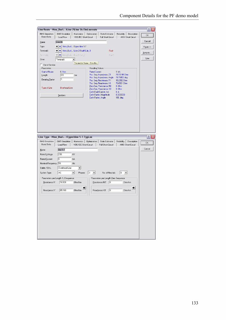
Component Details for the PF demo model

133

Component Details for the PF demo model

134

Line 3 – Details

Component Details for the PF demo model

135

Component Details for the PF demo model

136

Line 4 – Details

Component Details for the PF demo model

137

Component Details for the PF demo model

138

Line 5 – Details

Component Details for the PF demo model

139

Line 6 – Details

Component Details for the PF demo model

140

Component Details for the PF demo model

141

143

D MATLAB CALCULATIONS AND SCRIPTS

In this appendix the source code for the matlab calculations and plots introduced in the main rapport is available. Also the files are included in the attached CD at the folder.

• [CD-drive] :\Calculations\Matlab_Files \ … Illustration of droop Matlab code, droop.m: % % Purpose:illustrate droop % % Input: see paramters % % Output: plot of P and f relationship for droop controlled generator % % written 2009 as a part of MSc thesis % Kristjan P Petursson, stnr. s071538 %droop curve %parameters: R=0.05; %droop f_system=50; %system frequency %freq calculations delta_f=R*f_system; f_fullload=f_system-delta_f/2; f_noload=f_system+delta_f/2;; % load set, in pu. p_noload=0 % no load p_fullload=247.5 % full load %slope h=(f_fullload-f_noload) %x-values p=p_noload:1:p_fullload; %y-values f=f_noload+p.*h/p_fullload; %plot figure(1) clf %clears old graphics from figure figurenr=gcf; %gets number of created figure set(figurenr,'color',[1 1 1]) %sets colors of figure, all white plot(p,f) axis([p_noload p_fullload f_fullload-f_fullload*0.02 f_noload+f_noload*0.02]) title(['Relationship between power output and frequency. f_n_o_l_o_a_d=',num2str(f_noload),'Hz and f_f_u_l_l_l_o_a_d=',… num2str(f_fullload),'Hz']) xlabel('Generator Output, [pu]') ylabel('Frequency [Hz]')

Matlab Calculations and Scripts

144

Plot of ISR considering only steadty state frequency limits Matlab code, steadystateISR.m: % % Purpose:developing theoretical steady state frequency ISR region % % Input: see paramters % % Output: plot of the ISR based on steady state freq limits. % % written 2009 as a part of MSc thesis % Kristjan P Petursson, stnr. s071538 %assuming steady state is reached within 15 seconds. %Limits f_max = 50.2; %upper limit for allowed frequency. f_min = 49.8; %lower limit for allowed frequency. f_system = 50; %system frequency %parameters P_rated = 192+128; %total rated power within the island K_island = 192+85.33; %regulating const. for all generators in the island %calculation of Power limits P_export=(f_max-f_system)*K_island; P_import=(f_min-f_system)*K_island; %set X values, load as 0 to Prated load=0:1:P_rated; %syt Y values for limits for when island is en export mode P_lim_export = load+P_export; %syt Y values for limits for when island is en import mode P_lim_import = load+P_import; %plot limits figure(1) clf %clears old graphics from figure figurenr=gcf; %gets number of created figure set(figurenr,'color',[1 1 1]) %sets colors of figure, all white plot(load,P_lim_export,load,P_lim_import) axis([0 P_rated 0 P_rated]) title('Steady State Frequency Limits') ylabel('Power Generation pre-islanding [MW]') xlabel('Load [MW]') legend('Upper limit, Power export mode','lower limit, Power import mode'... ,'location','SouthEast')

Developing df/dt=f(H) Swing equation:

emam TTT

dtd

J −==ω

J is combined moment of inertia for generator and turbine [kg·m2] ωm is the angular velocity of the rotor [rad/s] Ta is the accelerating torque [N·m] Tm is the mechanical torque [N·m] Te is the electrical torque [N·m] J, Moment of inertia in terms of H(pu inertia)

Matlab Calculations and Scripts

145

basem

SHJ ⋅= 20

2ω

S is base value of appearant power H is inertia in pu sec P=T·ω and E=H·S

system

system

EfP

dtdf

⋅

⋅Δ=

2

∆P is change in power Analyzing frequency response of a system based on parameters, prime mover time constant (Ta), island system inertia (H) and generator controller droop (R) Also plot of ISR considering only steadty state frequency derivative limits for the given system parameters. Matlab code, freqDerivative.m: % script "freqDerivative.m" % % Purpose:1.analyse the freq. response with respect to different parameters % 2.define an ISR based on the frequency derivative criteria % % Input: see paramters % % Output: frequency response % % written 2009 as a part of MSc thesis % Kristjan P Petursson, stnr. s071538 %paramters %machine paramters Prated=[192 128]; % rated P Hgen=[4.125 2.765]; %inertia factor R=[2 3]; %droop in persentage case2 %other paramters fN=50; %system frequency Ta=0.2; %Ta time constant for prime mover dP=-10; t_step=0:0.002:10; %simulation time and stepseize, here limited %to 10 seconds dfdtcriteria=2.5; %critera for acceptable frequency derivative %Base values. Base values can be set here do represent results in pu. Sbase=1; %in MVA fbase=1; %Hz %Calculation of other base values Kbase = Sbase/fbase; %MW/HZ Hbase = 1/fbase; %Regulation constants for each machine, for k=1:length(Prated) K(k)=Prated(k)/R(k)/fN*100; end %Ksystem and frequency and power mismatch(in pu if base values are set in %paramters) Ksystempu=sum(K/Kbase); fNpu=fN/fbase; dPpu=dP/Sbase;

Matlab Calculations and Scripts

146

%Rotational energy of the system constant (p.u. if set) for k=1:length(Hgen) Erot(k)=Hgen(k)*Prated(k); %Kinetic energy of the system end Hsystem = sum(Erot)/sum(Prated); %System transfer function: %There are many ways to construct the transfer function, but I feel that %the following is the most illustrative, this is also how it is shown in %the report % The following notation is used % E(s) is the transfer function for inertia % F(s) is the transfer function for prime mover % G(s) is the transfer function for conotroller (gain) E=tf(1,[2*Hsystem 0] ); %inertia F=tf(1,[Ta 1]); %prime mover G=Ksystempu; %simple gain to represent the droop control H=E/(1+E*F*G) %the transfer function % % influence of the controller droop parameter, 3 settings tested %======================================================================== % normal droop E=tf(1,[2*Hsystem 0] ); F=tf(1,[Ta 1]); G=Ksystempu; H=E/(1+E*F*G) figure(1) clf %clears old graphics from figure figurenr=gcf; %gets number of created figure set(figurenr,'color',[1 1 1]) %sets colors of figure, all white [y,x]=step(fN+dPpu*H,t_step); subplot(2,1,1),plot(x,y,'g') % [temp1,temp2]=size(y); f_steady1=y(temp1,temp2); hold on %derivative a=makedfdt(y,x); subplot(2,1,2),plot(a(:,2),a(:,1),'g') peak1=max(abs(a(:,1))); hold on % increased droop Rpct=200; %droop increase to 200% for k=1:length(Prated) K(k)=Prated(k)/(R(k)*Rpct/100)/fN*100; end Ksystempu=sum(K/Kbase); E=tf(1,[2*Hsystem 0] ); F=tf(1,[Ta 1]); G=Ksystempu; H=E/(1+E*F*G) [y,x]=step(fN+dPpu/1*H,t_step); subplot(2,1,1),plot(x,y,'b') [temp1,temp2]=size(y); f_steady2=y(temp1,temp2); a=makedfdt(y,x); subplot(2,1,2),plot(a(:,2),a(:,1),'b') peak2=max(abs(a(:,1))); % %decreased droop Rpct=50; %droop increase to 50% for k=1:length(Prated) K(k)=Prated(k)/(R(k)*Rpct/100)/fN*100; end Ksystempu=sum(K/Kbase); E=tf(1,[2*Hsystem 0] );

Matlab Calculations and Scripts

147

F=tf(1,[Ta 1]); G=Ksystempu; H=E/(1+E*F*G) [y,x]=step(fN+dPpu*H,t_step); subplot(2,1,1),plot(x,y,'r') [temp1,temp2]=size(y); f_steady3=y(temp1,temp2); a=makedfdt(y,x); subplot(2,1,2),plot(a(:,2),a(:,1),'r') peak3=max(abs(a(:,1))); %plotting parameters, text and legends subplot(2,1,1),legend(['R \rightarrow f_s_t_e_a_d_y = ',num2str(f_steady1),'Hz'],['R\cdot200% \rightarrow f_s_t_e_a_d_y = ',num2str(f_steady2),'Hz'],['R\cdot50% \rightarrow f_s_t_e_a_d_y = ',num2str(f_steady3),'Hz'],'Location','SouthEast') subplot(2,1,2),legend(['R \rightarrow df/dt = ',num2str(peak1)],['R\cdot200% \rightarrow df/dt = ',num2str(peak2)],['R\cdot50% \rightarrow df/dt = ',num2str(peak3)],'Location','SouthEast') subplot(2,1,1),title(['Frequency Response when Due to Islanding Transition, \DeltaP = ',num2str(dP),' MW']) subplot(2,1,2),title(['Frequency Derivative for same Conditions']) subplot(2,1,2),xlabel('Time [s] - Islanding transition at t=0') subplot(2,1,1),ylabel('Frequency [Hz]') subplot(2,1,2),ylabel('Frequency [Hz]') hold off % % influence of the generator inertia, 3 settings tested %======================================================================== % normal inertia %resetting droop as set in parameters for k=1:length(Prated) K(k)=Prated(k)/R(k)/fN*100; end Ksystempu=sum(K/Kbase); E=tf(1,[2*Hsystem 0] ); F=tf(1,[Ta 1]); G=Ksystempu; %XXX H=E/(1+E*F*G) figure(2) clf %clears old graphics from figure figurenr=gcf; %gets number of created figure set(figurenr,'color',[1 1 1]) %sets colors of figure, all white [y,x]=step(fN+dPpu*H,t_step); subplot(2,1,1),plot(x,y,'g') % [temp1,temp2]=size(y); f_steady1=y(temp1,temp2); hold on %derivative a=makedfdt(y,x); subplot(2,1,2),plot(a(:,2),a(:,1),'g') peak1=max(abs(a(:,1))); hold on % increased inertia Hpct=200; %inertia increase to 200% for k=1:length(Hgen) Erot(k)=Hgen(k)*Hpct/100*Prated(k); %Kinetic energy of the system end Hsystem = sum(Erot)/sum(Prated); E=tf(1,[2*Hsystem 0] ); F=tf(1,[Ta 1]); G=Ksystempu; H=E/(1+E*F*G) [y,x]=step(fN+dPpu/1*H,t_step); subplot(2,1,1),plot(x,y,'b') [temp1,temp2]=size(y); f_steady2=y(temp1,temp2); a=makedfdt(y,x); subplot(2,1,2),plot(a(:,2),a(:,1),'b') peak2=max(abs(a(:,1)));

Matlab Calculations and Scripts

148

%decreased inertia Hpct=50; %inertia increase to 50% for k=1:length(Hgen) Erot(k)=Hgen(k)*Hpct/100*Prated(k); %Kinetic energy of the system end Hsystem = sum(Erot)/sum(Prated); E=tf(1,[2*Hsystem 0] ); F=tf(1,[Ta 1]); G=Ksystempu; H=E/(1+E*F*G) [y,x]=step(fN+dPpu*H,t_step); subplot(2,1,1),plot(x,y,'r') [temp1,temp2]=size(y); f_steady3=y(temp1,temp2); a=makedfdt(y,x); subplot(2,1,2),plot(a(:,2),a(:,1),'r') peak3=max(abs(a(:,1))); %plotting parameters, text and legends subplot(2,1,1),legend(['H \rightarrow f_s_t_e_a_d_y = ',num2str(f_steady1),'Hz'],['H\cdot200% \rightarrow f_s_t_e_a_d_y = ',num2str(f_steady2),'Hz'],['H\cdot50% \rightarrow f_s_t_e_a_d_y = ',num2str(f_steady3),'Hz'],'Location','SouthEast') subplot(2,1,2),legend(['H \rightarrow df/dt = ',num2str(peak1)],['H\cdot200% \rightarrow df/dt = ',num2str(peak2)],['H\cdot50% \rightarrow df/dt = ',num2str(peak3)],'Location','SouthEast') subplot(2,1,1),title(['Frequency Response when Due to Islanding Transition, \DeltaP = ',num2str(dP),' MW']) subplot(2,1,2),title(['Frequency Derivative for same Conditions']) subplot(2,1,2),xlabel('Time [s] - Islanding transition at t=0') subplot(2,1,1),ylabel('Frequency [Hz]') subplot(2,1,2),ylabel('Frequency [Hz]') subplot(2,1,1),axis([0 10 49.5 50.2]) subplot(2,1,2),axis([0 10 -3 2.5]) hold off % % influence of the prime mover time constant Ta, 3 settings tested %======================================================================== %Normal prime mover time constant Ta %Resetting inertia as set in parameters for k=1:length(Hgen) Erot(k)=Hgen(k)*Prated(k); %Kinetic energy of the system end Hsystem = sum(Erot)/sum(Prated); E=tf(1,[2*Hsystem 0] ); F=tf(1,[Ta 1]); G=Ksystempu; %XXX H=E/(1+E*F*G) figure(3) clf %clears old graphics from figure figurenr=gcf; %gets number of created figure set(figurenr,'color',[1 1 1]) %sets colors of figure, all white [y,x]=step(fN+dPpu*H,t_step); subplot(2,1,1),plot(x,y,'g') [temp1,temp2]=size(y); f_steady1=y(temp1,temp2); hold on %derivative a=makedfdt(y,x); subplot(2,1,2),plot(a(:,2),a(:,1),'g') peak1=max(abs(a(:,1))); hold on % increased prime mover time constant Ta Tapct=200; %Ta increase to 200% E=tf(1,[2*Hsystem 0] ); F=tf(1,[Ta*Tapct/100 1]); G=Ksystempu; H=E/(1+E*F*G) [y,x]=step(fN+dPpu/1*H,t_step); subplot(2,1,1),plot(x,y,'b') [temp1,temp2]=size(y); f_steady2=y(temp1,temp2);

Matlab Calculations and Scripts

149

a=makedfdt(y,x); subplot(2,1,2),plot(a(:,2),a(:,1),'b') peak2=max(abs(a(:,1))); %decreased prime mover time constant Ta Tapct=50; %Ta increase to 50% E=tf(1,[2*Hsystem 0] ); F=tf(1,[Ta*Tapct/100 1]); G=Ksystempu; H=E/(1+E*F*G) [y,x]=step(fN+dPpu*H,t_step); subplot(2,1,1),plot(x,y,'r') [temp1,temp2]=size(y); f_steady3=y(temp1,temp2); a=makedfdt(y,x); subplot(2,1,2),plot(a(:,2),a(:,1),'r') peak3=max(abs(a(:,1))); %plotting parameters, text and legends subplot(2,1,1),legend(['T_a \rightarrow f_s_t_e_a_d_y = ',num2str(f_steady1),'Hz'],['T_a\cdot200% \rightarrow f_s_t_e_a_d_y = ',num2str(f_steady2),'Hz'],['T_a\cdot50% \rightarrow f_s_t_e_a_d_y = ',num2str(f_steady3),'Hz'],'Location','SouthEast') subplot(2,1,2),legend(['T_a \rightarrow df/dt = ',num2str(peak1)],['T_a\cdot200% \rightarrow df/dt = ',num2str(peak2)],['T_a\cdot50% \rightarrow df/dt = ',num2str(peak3)],'Location','SouthEast') subplot(2,1,1),title(['Frequency Response when Due to Islanding Transition, \DeltaP = ',num2str(dP),' MW']) subplot(2,1,2),title(['Frequency Derivative for same Conditions']) subplot(2,1,2),xlabel('Time [s] - Islanding transition at t=0') subplot(2,1,1),ylabel('Frequency [Hz]') subplot(2,1,2),ylabel('Frequency [Hz]') subplot(2,1,1),axis([0 10 49.5 50.2]) subplot(2,1,2),axis([0 10 -3 2.5]) hold off % % ISR based on df/dt criteria %======================================================================== %reset the transfer function for the system: for k=1:length(Prated) K(k)=Prated(k)/R(k)/fN*100; end Ksystempu=sum(K/Kbase); fNpu=fN/fbase; dPpu=dP/Sbase; %Rotational energy of the system constant (p.u. if set) for k=1:length(Hgen) Erot(k)=Hgen(k)*Prated(k); %Kinetic energy of the system end Hsystem = sum(Erot)/sum(Prated); E=tf(1,[2*Hsystem 0] ); %inertia F=tf(1,[Ta 1]); %prime mover G=Ksystempu; %simple gain to represent the droop control H=E/(1+E*F*G) %the transfer function %set power mismatch array dPvar=0:0.1:sum(Prated); %find limits when island is in import mode flag=0; %flag for when system is no longer within criteria k=1; %counter while flag ==0 && k<length(dPvar) [y,x]=step(fN+dPvar(k)*H,t_step); a=makedfdt(y,x); %calculate the derivative peak=max(abs(a(:,1))); %get absolute highest value of df/dt if peak > dfdtcriteria flag = 1; k=k-1; %minus here only to compensate for last %count after max value has been found [temp1,temp2]=size(y); %register steady state freq

Matlab Calculations and Scripts

150

f_steady=y(temp1,temp2); end k=k+1; end P_export=dPvar(k); disp(['(export mode) Max dP = ',num2str(dPvar(k)),... ' resulting in max df/dt = ',num2str(peak),... ' and steady state frequency f = ',num2str(f_steady)]) %finding the lower limit, when island is in export mode flag=0; %flag for when system is no longer witin criteria k=1; %counter dPvar=dPvar*(-1); while flag ==0 && k<length(dPvar) [y,x]=step(fN+dPvar(k)*H,t_step); a=makedfdt(y,x); %calculate the derivative peak=max(abs(a(:,1))); %get absolute highest value of df/dt if peak > dfdtcriteria flag = 1; k=k-1; %minus here only to compensate for last % count after max value has been found [temp1,temp2]=size(y); %register steady state freq f_steady=y(temp1,temp2); end k=k+1; end P_import=dPvar(k); disp(['(import mode) Max dP = ',num2str(dPvar(k)),... ' resulting in max df/dt = ',num2str(peak),... ' and steady state frequency f = ',num2str(f_steady)]) %plot the ISR limits based on above %set X values, load as 0 to Prated load=0:1:sum(Prated); %syt Y values for limits for when island is en export mode P_lim_export = load+P_export; %syt Y values for limits for when island is en import mode P_lim_import = load+P_import; %plot limits figure(1) clf %clears old graphics from figure figurenr=gcf; %gets number of created figure set(figurenr,'color',[1 1 1]) %sets colors of figure, all white plot(load,P_lim_export,load,P_lim_import) axis([0 sum(Prated) 0 sum(Prated)]) title('Frequency Derivative Limits') ylabel('Power Generation pre-islanding [MW]') xlabel('Load [MW]') legend('Upper limit, Power export mode','Lower limit, Power import mode'... ,'location','SouthEast')

151

E CONTENTS OF ATTACHED CD

Contents of CD

• Calculations Plot_3curves.fig Steadystate_ISR.m Droop.m freqDerivative.m freqdev.m madedfdt.m maxdfdt.m

• Project Report Influence of Different Generation on ISR.docx Influence of Different Generation on ISR.pdf

• Simulations o Matlab Script functions

evaluateISR.m freqdev.m freqtime.m maxdfdt.m outlineMatrix3D.m outlineMatrix.m paraChangeCounter.m peakFreq.m plot3DISR.m plot2DISR.m plotISR.m plotSimple.m read_txt.m returnIndexed.m sortMatrix.m test_of_stablematrix.m volttime.m

o PF-projects

Contents of Attached CD

152

9bus – aggregation.dz 9bus – DFR.dz 9bus – dispatch.dz 9bus – droop.dz 9bus – load shedding.dz 9bus – prime mover.dz 9bus – reference model.dz 9bus – inertia.dz 9bus – WT.dz

www.elektro.dtu.dk/cet Department of Electrical Engineering Centre for Electric Technology (CET) Technical University of Denmark Elektrovej 325 DK-2800 Kgs. Lyngby Denmark Tel: (+45) 45 25 35 00 Fax: (+45) 45 88 61 11 E-mail: cet@elektro.dtu.dk [Skriv: ISBN XX-XXXXX-XX-X (eller slet)]