MGMT90141 Business Analysis and Decision Making Week 1 ... · MGMT90141 Business Analysis and...

MGMT90141 Business Analysis and Decision MakingWeek 1 – Introduction to Business Analytics and Linear Programming

Dr. William Ho

Associate Professor of Operations ManagementDepartment of Management and MarketingFaculty of Business and EconomicsThe Spot [email protected]

• 10 lectures and tutorials + 1 revision + 1 class presentations

• 2 recommended textbooks– Anderson, D.R., Sweeney, D.J., Williams, T.A., Camm, J.D.,

and Martin, K. (2014), An Introduction to Management Science: Quantitative Approaches to Decision Making, 14th edition, South-Western Cengage Learning

– Anderson, D.R., Sweeney, D.J., Williams, T.A., Camm, J.D., and Cochran, J. (2014), Statistics for Business Economics, 12th edition, South-Western Cengage Learning

• LMS– Lecture slides– All subject related documents

Studying for MGMT90141

• Each week– Prepare for lecture and tutorial:

• Read through equivalent book chapter(s)– After lecture and tutorial:

• Re-read, try problems for any part of lecture and tutorialwhich is not clear

• Try to apply the quantitative methods in real situations• Discuss with your subject coordinator if you found any

interesting and/or difficult subject-related matters

• Assessments– A 2000 word group assignment, due Week 5 (15%)– A 4000 word group assignment, due Week 11 (30%)– A 10 minute oral presentation, due Week 12 (5%)– A 2-hour closed book examination, end of semester (50%)

Studying for MGMT90141

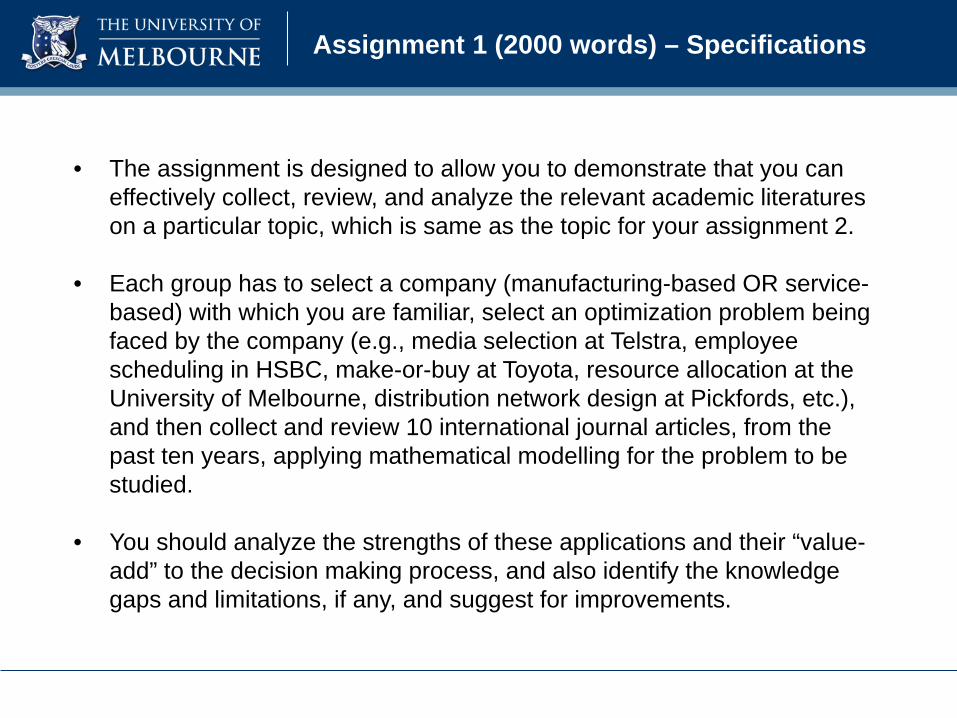
Assignment 1 (2000 words) – Specifications

• The assignment is designed to allow you to demonstrate that you can effectively collect, review, and analyze the relevant academic literatures on a particular topic, which is same as the topic for your assignment 2.

• Each group has to select a company (manufacturing-based OR service-based) with which you are familiar, select an optimization problem being faced by the company (e.g., media selection at Telstra, employee scheduling in HSBC, make-or-buy at Toyota, resource allocation at the University of Melbourne, distribution network design at Pickfords, etc.), and then collect and review 10 international journal articles, from the past ten years, applying mathematical modelling for the problem to be studied.

• You should analyze the strengths of these applications and their “value-add” to the decision making process, and also identify the knowledge gaps and limitations, if any, and suggest for improvements.

Assignment 1 – Expected Contents of Report

• Introduction – company background, description of the business optimization problem, justification of selection, identification of the company’s requirements or evaluation criteria, etc.

• Methodology – description of the method used to collect the journal articles, such as databases, searching and filtering criteria, etc.

• Strengths – analysis of the strengths of the articles with respect to the evaluation criteria.

• Weaknesses – analysis of the weaknesses of the articles with respect to the evaluation criteria.

• Discussions and Conclusions – suggestions for improvement.

• References

• Appendices – including the minutes/notes of meetings.

Assignment 1 – Marking Criteria

Criteria Possible Mark

Identification and description of the problem to be analyzed

2

Collection and discussion of relevant academic literatures 3

Analysis of the strengths of these applications and their “value-add” to the decision making process

4

Identification of the knowledge gaps and limitations, if any, and suggestion for improvements

4

Structure and presentation. Use of appropriate language, spelling, grammar, and punctuation

2

Total 15

Assignment 1 – Word Limits and Submission Due

• Word limits – The total length of the report is a maximum of 2,000 words (excluding figures, tables, references, and appendices).

• Submission due – 5pm 20 August 2018

Assignment 1 – Useful Online Sources

• http://ieeexplore.ieee.org/Xplore/home.jsp

• http://www.emeraldlibrary.com

• http://www.ingentaconnect.com

• http://www.sciencedirect.com

• http://www.scopus.com

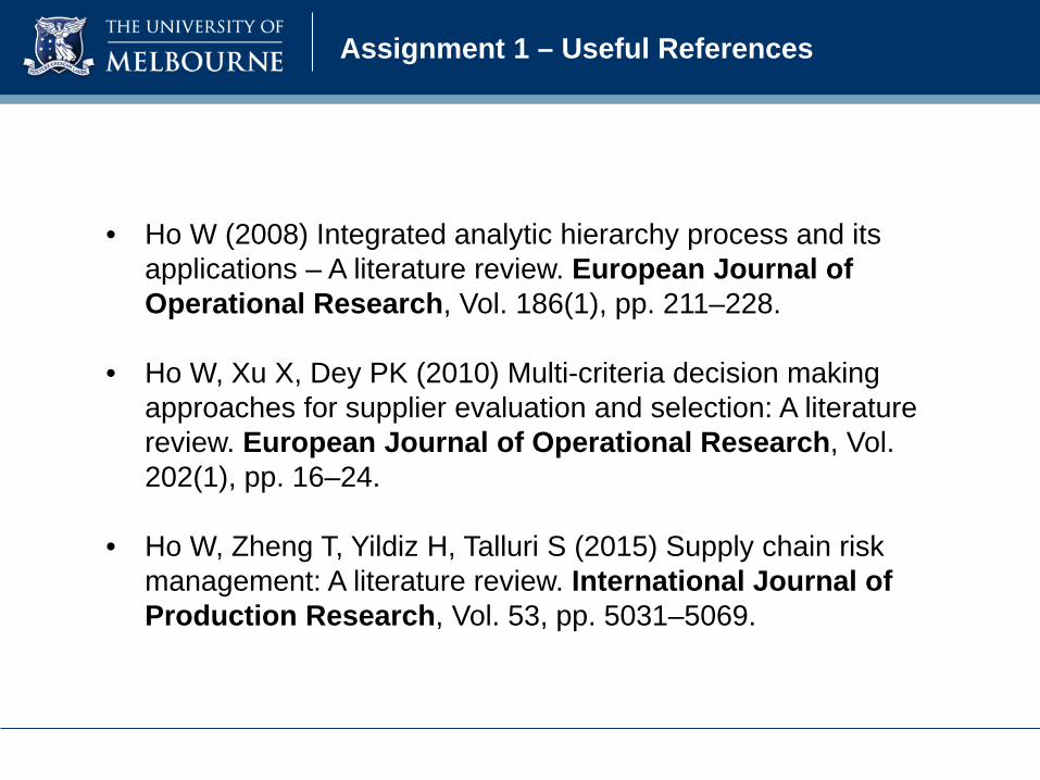
Assignment 1 – Useful References

• Ho W (2008) Integrated analytic hierarchy process and its applications – A literature review. European Journal of Operational Research, Vol. 186(1), pp. 211–228.

• Ho W, Xu X, Dey PK (2010) Multi-criteria decision making approaches for supplier evaluation and selection: A literature review. European Journal of Operational Research, Vol. 202(1), pp. 16–24.

• Ho W, Zheng T, Yildiz H, Talluri S (2015) Supply chain risk management: A literature review. International Journal of Production Research, Vol. 53, pp. 5031–5069.

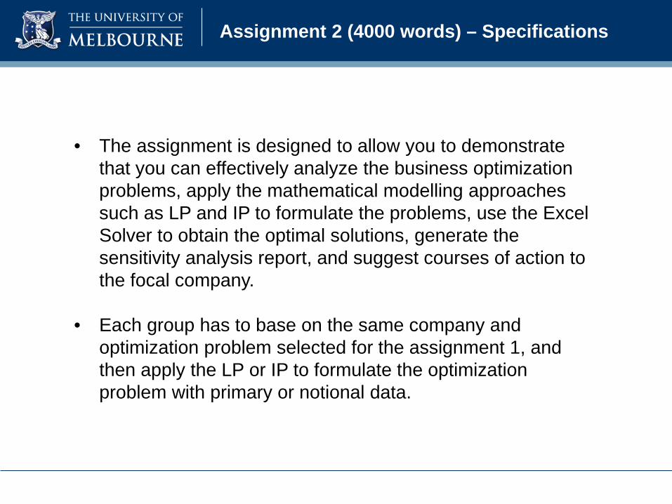
Assignment 2 (4000 words) – Specifications

• The assignment is designed to allow you to demonstrate that you can effectively analyze the business optimization problems, apply the mathematical modelling approaches such as LP and IP to formulate the problems, use the Excel Solver to obtain the optimal solutions, generate the sensitivity analysis report, and suggest courses of action to the focal company.

• Each group has to base on the same company and optimization problem selected for the assignment 1, and then apply the LP or IP to formulate the optimization problem with primary or notional data.

Assignment 2 – Expected Contents of Report

• Introduction – company background, description of the business optimization problem, justification of selection, etc.

• Literature review – summary of the findings from the assignment 1.

• Methodology – description and illustration of the mathematical modelling approach for the problem.

• Implementation – formulation of the problem by using the mathematical modelling approach, application of the Excel Solver to optimize the mathematical model, and execution of the sensitivity analysis.

• Discussions and Conclusions – suggestions for courses of action to the selected company as well as the evaluation of the mathematical modelling approach.

• References

• Appendices – including the minutes/notes of meetings.

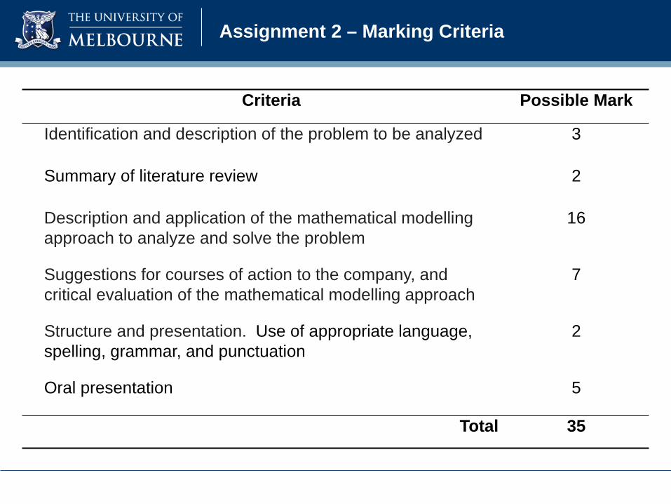
Assignment 2 – Marking Criteria

Criteria Possible Mark

Identification and description of the problem to be analyzed 3

Summary of literature review 2

Description and application of the mathematical modellingapproach to analyze and solve the problem

16

Suggestions for courses of action to the company, and critical evaluation of the mathematical modelling approach

7

Structure and presentation. Use of appropriate language, spelling, grammar, and punctuation

2

Oral presentation 5

Total 35

Assignment 2 – Word Limits and Submission Due

• Word limits – The total length of the report is a maximum of 4,000 words (excluding figures, tables, references, and appendices).

• Submission due – 5pm 8 October 2018

• Part one (25%): 1 compulsory question

• Part two (75%): 3 out of 4 questions

• All questions are equally weighted

Note: Successful completion of this subject requires a pass (50%) in the final exam.

Examination

• To explain what is business analytics

• To introduce the linear programming elements, formulation, and solution approaches

• To differentiate between the minimization and maximization linear programming problems

• To recognize the sensitivity analysis of the linear programming models

Objectives of Lecture

• The use of data, information technology, statistical analysis, quantitative methods, and mathematical or computer-based models to help managers gain improved insight about their business operations and make better, fact-based decisions

• Supported by various tools such as Microsoft Excel and various Excel add-ins, commercial statistical software packages such as SAS or SPSS, and more complex business intelligence suites that integrate data with analytical software.

Business Analytics – Introduction

• Descriptive: categorize, characterize, consolidate and classify data to convert it into useful information for the purposes of understanding and analysing past and current business performance and make informed decisions.

• Predictive: analyze past performance in an effort to predict the future by examining historical data, detecting patterns or relationships in these data, and then extrapolating these relationships forward in time.

• Prescriptive: use optimization to identify the best alternatives to minimize or maximize a single or multiple objective. The mathematical and statistical techniques of predictive analytics can also be combined with optimization to make decisions that take into consideration the uncertainty in the data.

Business Analytics – Elements

• In the world of management science or operations research, programming refers to modelling and solving a problem mathematically.

• LP is widely used mathematical technique designed to help managers plan and make the decisions necessary to allocate resources.

• Many business decisions involve trying to make the most effective use of an organization’s resources. Resources typically include machinery, labour, money, time, and raw materials. These resources may be used to produce products or services.

Linear Programming – Introduction

• A set of decision variables: which are used to stand for the quantity of each product or service to be produced.

• An objective function: which measures the extent to which alternative feasible decisions achieve the aim being pursued.

• A set of constraints: which define in mathematical terms the values of the decision variables that are feasible.

Linear Programming – Elements

Max or Min c1x1 + c2x2 + … + cnxn

Subject to: a11x1 + a12x2 + … + a1nxn ≤ b1a21x1 + a22x2 + … + a2nxn ≤ b2………………………………………

am1x1 + am2x2 + … + amnxn ≤ bm

All x1, …, xn ≥ 0.

c1, …, cn: Objective function coefficientsa11, …, amn: Technical coefficientsb1, …, bm: Right-hand-sides (RHS)x1, …, xn: Decision variables

Linear Programming – General Form

• Deterministic model

– All ci, aij, bj (for i = 1, …, n; j = 1, …, m) are known with certainty.

• Implications of linearity

– Divisibility: All variables are continuous. For example, we could produce whole tons of products or proportions of tons.

– Proportionality: Value of the function is in direct proportion to the values of the decision variables. For example, if we increase the cost per unit shipped by 10%, then we will increase the total cost of the shipments by 10% .

Linear Programming – Assumptions

The Shader Electronics Company produces two products: (1) the Shader x-pod, a portable music player, and (2) the Shader BlueBerry, an internet-connected colour telephone. The production process for each product is similar in that both require a certain number of hours of electronic work and a certain number of labour-hours in the assembly department. Each x-pod takes 4 hours of electronic work and 2 hours in the assembly shop. Each BlueBerry requires 3 hours in electronics and 1 hour in assembly. During the current production period, 240 hours of electronic time are available, and 100 hours of assembly department time are available. Each x-pod sold yields a profit of $7; each BlueBerry produced can be sold for a $5 profit.

Shader’s problem is to determine the best possible combination of x-pods and BlueBerrys to manufacture to reach the maximum profit.

Linear Programming – Maximization

Step 1: Fully understand the managerial or optimization problem being faced

Hours required to produce one unit

Department x-pods BlueBerrys Available hours

Electronic 4 3 240

Assembly 2 1 100

Profit per unit $7 $5

How many x-pods and BlueBerrys should Shader manufacture to reach the maximum profit, while not exceeding the limited amount of electronic and assembly time?

Linear Programming – Formulation

Step 2: Define the decision variables

x1 = number of x-pods to be producedx2 = number of BlueBerrys to be produced

Step 3: Identify the objective function

Maximize profit or z = 7x1 + 5x2

Step 4: Identify the constraints

4x1 + 3x2 ≤ 240 (Electronic department resource constraint)2x1 + 1x2 ≤ 100 (Assembly department resource constraint)x1 and x2 ≥ 0 (Non-negativity)


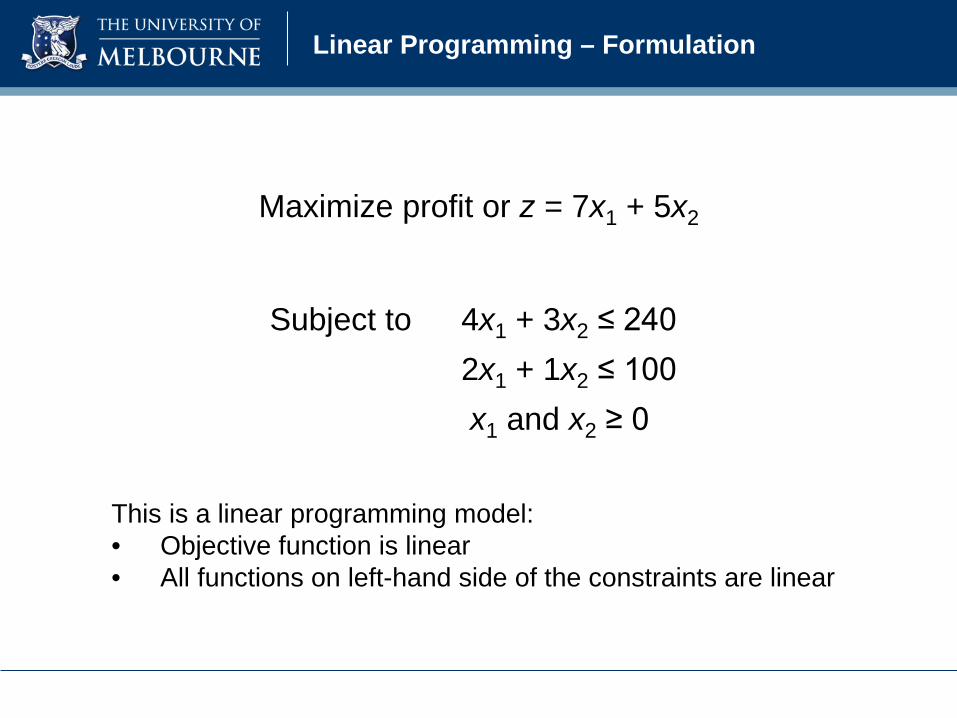
Maximize profit or z = 7x1 + 5x2

Subject to 4x1 + 3x2 ≤ 2402x1 + 1x2 ≤ 100x1 and x2 ≥ 0

This is a linear programming model:• Objective function is linear• All functions on left-hand side of the constraints are linear


• Graphical Solution Method:– Plot the solution on a two-dimensional graph

• Simplex Method:– It is the basis of most LP optimization software. It works by finding corner point solutions, evaluating the objective function at each, and stopping when no more improvement to the objective function value (z) is possible.

• Optimization Software:– such as Lindo, SAS etc.

• MS Excel:– Solver add-in is needed.

Linear Programming – Solution

• A free (limited) version can be downloaded from http://www.lindo.com

• Once the software is running, the first window is untitled. You should enter your model in this window and then save, naming the file as you wish.

• For the Shader problem the input file is:

Linear Programming – Lindo

http://www.lindo.com/

• When this has been saved, proceed as follows:– Click “Debug” in “Solve” submenu to debug any errors– When no more errors, click “Solve” in “Solve” submenu– Answer “No” to the question: “Do Range (Sensitivity) Analysis?”– To view the solution, Click “Solution” in “Reports” submenu

Linear Programming – Lindo

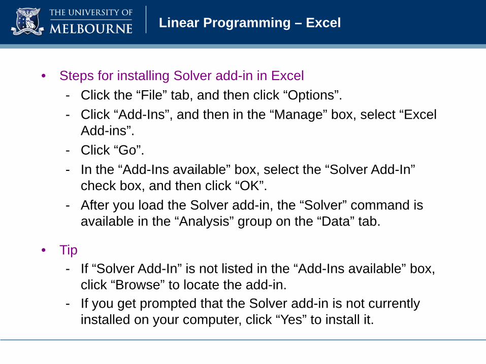
• Steps for installing Solver add-in in Excel- Click the “File” tab, and then click “Options”.- Click “Add-Ins”, and then in the “Manage” box, select “Excel

Add-ins”.- Click “Go”.- In the “Add-Ins available” box, select the “Solver Add-In”

check box, and then click “OK”.- After you load the Solver add-in, the “Solver” command is

available in the “Analysis” group on the “Data” tab.

• Tip- If “Solver Add-In” is not listed in the “Add-Ins available” box,

click “Browse” to locate the add-in.- If you get prompted that the Solver add-in is not currently

installed on your computer, click “Yes” to install it.

Linear Programming – Excel

• Data Input

=SUMPRODUCT(B7:C7,B12:C12)

=SUMPRODUCT(B4:C4,B12:C12) =SUMPRODUCT(B5:C5,B12:C12)


• Parameters setting(Data > Solver)

Enter the cell address for the objective function value.

Specify the location of the values for the variables. Solver will put the optimal values here.

Click “Add” to add the constraints to Solver.

Check this box to make the variables non-negative.

Click and select “Simplex LP” from the menu that appears.Check “Solve” to solve the LP.


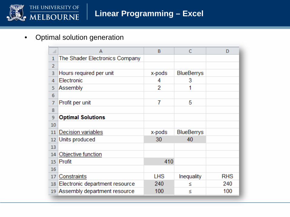
• Optimal solution generation


• Changes in the objective function coefficients- Reduced cost: how much the objective function coefficient of each

decision variable would have to improve before that variable could assume a positive value in the optimal solution.

- Allowable increase and decrease: what are the limits that the objective function coefficients can be adjusted without affecting the optimality of the current solution.

• Changes in the constraints or right-hand-side (RHS) values- Shadow price or dual prices (in Lindo): how much objective function

value can be improved if the RHS value of a constraint is increased by one unit.

- Allowable increase and decrease: what are the limits that RHS value of a constraint can be adjusted without affecting the validity of the shadow price.

Linear Programming – Sensitivity Analysis

• For Lindo, in the “Reports” submenu, click “Solution”.• In the “Reports” submenu, click “Range”.


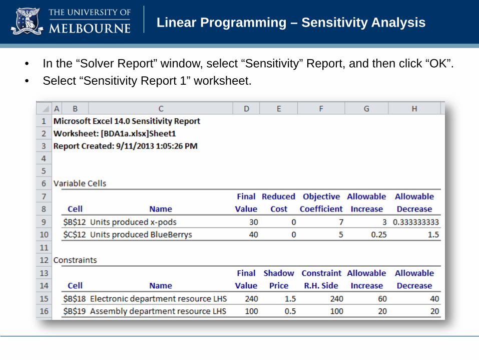
• In the “Solver Report” window, select “Sensitivity” Report, and then click “OK”.• Select “Sensitivity Report 1” worksheet.


As part of a quality improvement initiative, Consolidated Electronics employees complete a 3-day training program on teaming and a 2-day training program on problem solving. The manager of quality improvement has requested that at least 8 training programs on teaming and at least 10 training programs on problem solving be offered during the next 3 months. In addition, senior-level management has specified that at least 25 training programs must be offered during this period. Consolidated Electronics uses a consultant to teach the training programs. During the next 3 months, the consultant has 84 days of training time available. Each training program on teaming costs $10,000 and each training program on problem solving costs $8,000.

Consolidated Electronics’s problem is to determine the number of training programs on teaming and the number of training programs on problem solving that should be offered in order to minimize the total cost.

Linear Programming – Minimization

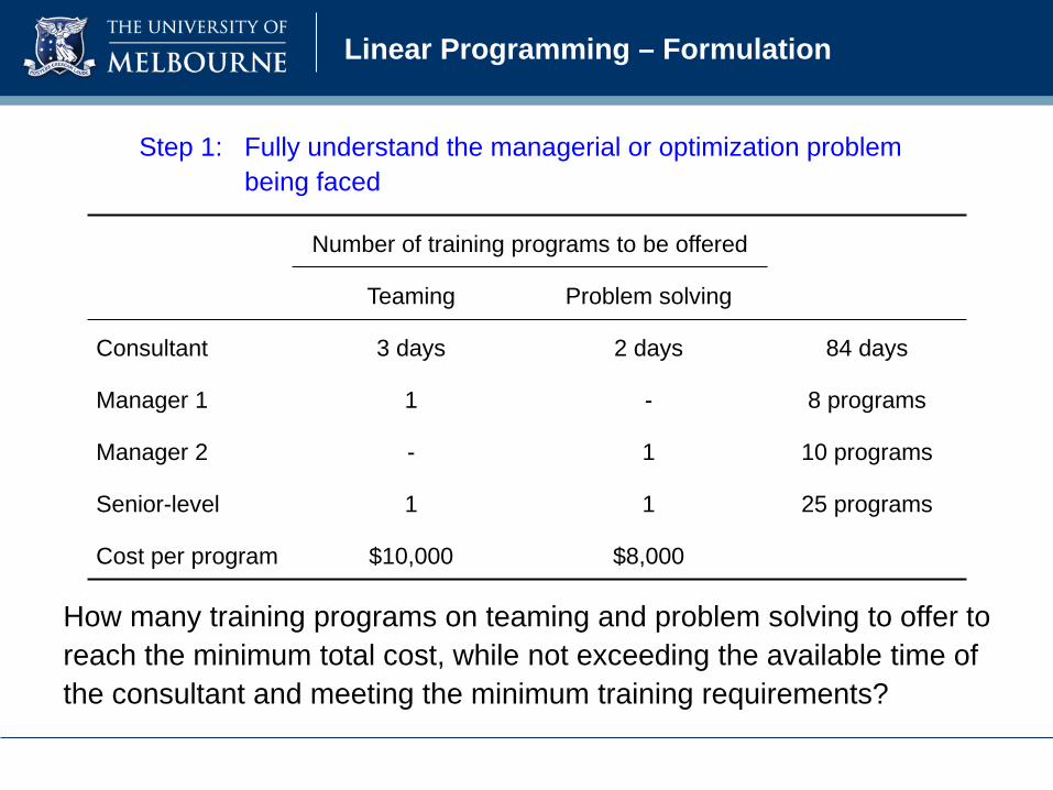
Step 1: Fully understand the managerial or optimization problem being faced

Number of training programs to be offered

Teaming Problem solving

Consultant 3 days 2 days 84 days

Manager 1 1 - 8 programs

Manager 2 - 1 10 programs

Senior-level 1 1 25 programs

Cost per program $10,000 $8,000

How many training programs on teaming and problem solving to offer to reach the minimum total cost, while not exceeding the available time of the consultant and meeting the minimum training requirements?


Step 2: Define the decision variables

Step 3: Identify the objective function

Step 4: Identify the constraints


• Data Input

Linear Programming – Excel Solution

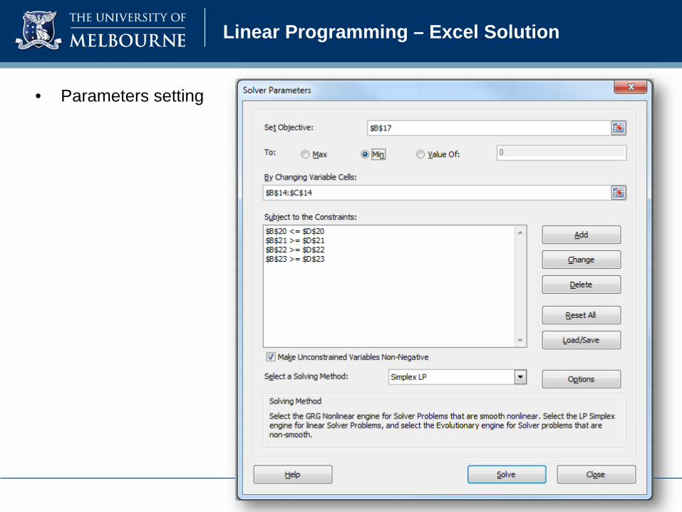
• Parameters setting


• Optimal solution generation


• Sensitivity analysis


Failsafe Electronics Corporation primarily manufactures four highly technical products, which it supplies to aerospace firms that hold NASA contracts. Each of the products must pass through the following departments before they are shipped: wiring, drilling, assembly, and inspection. The time requirements in each department (in hours) for each unit produced and its corresponding profit value are summarized below:

Department

Product Wiring Drilling Assembly Inspection Unit Profit

XJ201 0.5 3 2 0.5 $9

XM897 1.5 1 4 1 $12

TR29 1.5 2 1 0.5 $15

BR788 1 3 2 0.5 $11

Tutorial

The production time available in each department each month and the minimum monthly production requirement to fulfill contracts are as follows:

Failsafe Electronics Corporation’s problem is to determine the production quantities of the four highly technical products in order to maximize the total profit.

Department Capacity (hours) Product Minimum production level

Wiring 1,500 XJ201 150

Drilling 2,350 XM897 100

Assembly 2,600 TR29 200

Inspection 1,200 BR788 400

Tutorial

Summary of Lecture

• Explained what is business analytics

• Introduced the linear programming elements, formulation, and solution approaches

• Differentiated between the minimization and maximization linear programming problems

• Recognized the sensitivity analysis of the linear programming models

1) Readings– Chapters 2 and 3 (An Introduction to

Management Science: Quantitative Approaches to Decision Making)

2) Useful websites– http://www.theorsociety.com/– https://www.informs.org/– http://ifors.org/web/

Announcements

MGMT90141 Business Analysis and Decision Making Week 1 ... · MGMT90141 Business Analysis and...

Documents

Transcript of MGMT90141 Business Analysis and Decision Making Week 1 ... · MGMT90141 Business Analysis and...