MFE8812 Bond Portfolio Management - Nanyang …2p… · Bond Prices and Yields Measurement of...

Bond Prices and YieldsMeasurement of Interest Rate Risk

MFE8812 Bond Portfolio Management

William C. H. Leon

Nanyang Business School

January 16, 2018

1 / 63 William C. H. Leon MFE8812 Bond Portfolio Management


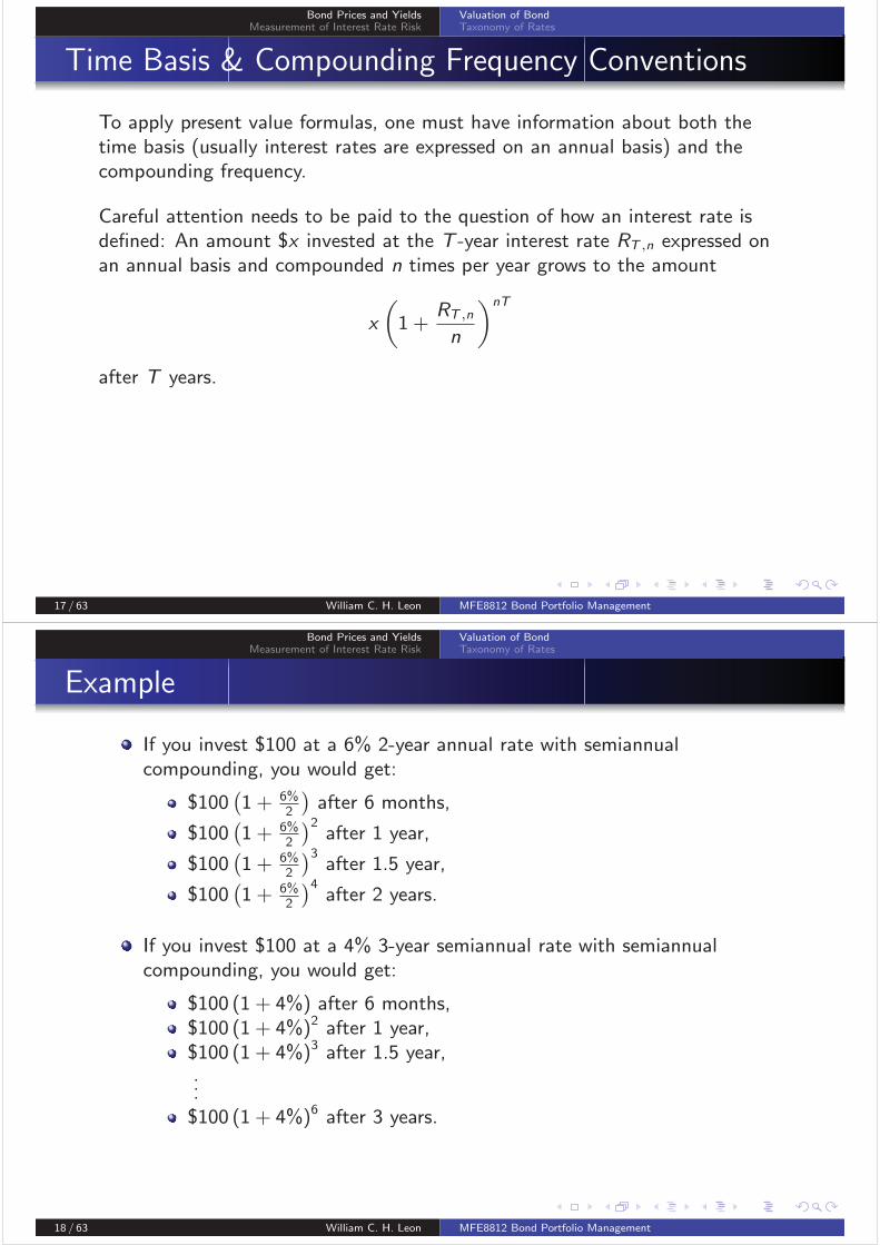
1 Bond Prices and YieldsOverview

Valuation of BondValue of Cash FlowsValue of a BondPresent Value Formula

Taxonomy of Rates

2 Measurement of Interest Rate RiskOverview

Full Valuation Approach

Duration & Convexity Approach



Valuation of BondTaxonomy of Rates

Overview

Bond pricing is typically performed by taking the discounted value of thebond cash flows.

We shall review the basics of the mathematics of discounting, includingtime basis and compounding conventions, and introduce various types ofinterest rates involved in the fixed-income world, including the notions ofcoupon rate, current yield, yield to maturity, spot rate, forward rate andbond par yield.




Present Value of a Cash Flow

Consider a cash flow CFT that occurs at time T :

Time t0

Present1 2 3 . . . T

Future

Discount rate rT

Cash Flow CFT

CFTPV =CFT

(1 + rT )T




Present Value of a Stream of Cash Flows

Consider a stream of cash flow CF1,CF2,CF3, . . . ,CFT :

Time t0

Present1 2 3

. . .

. . . TFuture

Discount rate rt for maturity t

CFTCF3CF2CF1

PV =CF1

1 + r1+

CF2

(1 + r2)2+

CF3

(1 + r3)3+ · · ·+

CFT

(1 + rT )T=

T∑t=1

CFt

(1 + rt)t.




Valuing a Bond

Valuing a bond can be viewed as a three-step process:

Step 1: obtain the cash flows the bondholder is entitled to.

Step 2: obtain the discount rates for the maturities corresponding to thecash flow dates.

Step 3: obtain the bond price as the discounted value of the cash flows.




Obtaining Cash Flows of a Bond

If we are dealing with a straight default-free, fixed-coupon bond, the valueof cash flows paid by the bond are known with certainty ex ante, i.e., onthe date when pricing is performed.

In general, two parameters that are needed to fully describe the cash flowson a bond.

The first is the maturity date of the bond, on which the principal orface amount of the bond is paid and the bond retired.The second parameter needed to describe a bond is the coupon rate.

For a non-standard bond, the following are some of the problemsassociated with estimating cash flows:

The due date for the payment of the principal may be altered.The coupon payments may be reset periodically.There may be an option to convert or exchange one security foranother security.




Example

A Canadian Government bond issued in the domestic market pays one-half ofits coupon rate times its principal value every 6 months up to and including thematurity date. Thus, a bond with an 8% coupon and $5,000 face valuematuring on December 1, 2xx5, will make future coupon payments of 4% ofprincipal value, that is, $200 on every June 1 and December 1 between thepurchase date and the maturity date.




Obtaining Discount Rates

Given that the cash flows are known with certainty ex ante, only the time-valueneeds to be accounted for, using the present value rule, which can be writtenas the follow

PV (CFt) =CFt(

1 + R(0, t))t = B(0, t)CFt ,

where PV (CFt) is the present value of the cash flow CFt received at date t,R(0, t) is the annual spot rate (or discount rate) at date 0 for an investment upto date t, and B(0, t) is the price at date 0 (today) of a zero-coupon bond (orpure discount bond) paying $1 on date t.

Note that it would be easy to obtain B(0, t) if we can find zero-coupon bondscorresponding to all possible maturities.




Obtaining Bond Price

The price of a bond

P0 = PV (Bond) =

T∑t=1

CFt(1 + R(0, t)

)t =

T∑t=1

B(0, t)CFt .

We must address the following important issues to turn the above simpleprinciple into sound practice:

Where do we get the discount factors B(0, t) from?

Do we use the equation to obtain bond prices or implied discount factors?

Can we deviate from this simple rule? Why?




Mathematics of Discounting

Suppose that all cash flows and all discount rates across various maturities areidentical and, respectively, equal to CF and y . Then

PV

(T∑t=1

CF

)=

T∑t=1

CF(1 + y

)t =CF

y

(1−

1(1 + y

)T).

For a bond, we have

P0 =C

y

(1−

1(1 + y

)T)

+N(

1 + y)T .

where P0 is the present value of the bond, T is the maturity of the bond, N isthe nominal value of the bond, C = c × N is the coupon payment, c is thecoupon rate and y is the discount rate.




Example

Consider the problem of valuing a bond with a 5% coupon rate, annual couponpayments, a 10-year maturity and a $1,000 face value; assuming all discountrates equal to 6%.

Step 1: The cash flows of the bond is

CF1 = CF2 = · · · = CF9 = $50 and CF10 = $1, 050.

Step 2: The discount rate y = 0.06.

Step 3: The value of the bond is

P0 =

9∑t=1

50

1.06t+

1050

1.0610=

50

0.06

(1−

1

1.0610

)+

1000

1.0610

= $926.39913.




Priced at Par

When the coupon rate is equal to the discount rate (i.e., c = y or equivalentlyC = y N), then the bond value is equal to its face value.

P0 =c N

y

(1−

1(1 + y

)T)

+N(

1 + y)T

=y N

y

(1−

1(1 + y

)T)

+N(

1 + y)T = N.




Premium, Par & Discount

More generally, depending on the relation between coupon rate, c, anddiscount rate, y , a bond may be priced:

at a premium, P0 > N;

at par, P0 = N; or

at a discount, P0 < N.

P0 = N

(c

y

(1−

1(1 + y

)T)

+1(

1 + y)T

),

c > y P0 > N, i.e., at a premium

c = y P0 = N, i.e., at par

c < y P0 < N, i.e., at a discount




Perpetual Bond

A bond paying a given coupon amount every year over an unlimited horizon isknown as a perpetual bond. The price of such bond is

P0 = limT→∞

T∑t=1

C(1 + y

)t = limT→∞

C

y

(1−

1(1 + y

)T)

=C

y.




Annual vs. Semiannual Coupons

Consider a bond with a coupon rate c, a maturity T year, a face value N, anda discount rate y .

If the bond delivers coupon annually, its price

P0 =

T∑t=1

c N(1 + y

)t +N(

1 + y)T =

c N

y

(1−

1(1 + y

)T)

+N(

1 + y)T .

If the bond delivers coupon semiannually, its price

P0 =

2T∑t=1

c N/2(1 + y/2

)t +N(

1 + y/2)2T

=c N

y

(1−

1(1 + y/2

)2T)

+N(

1 + y/2)2T .




Time Basis & Compounding Frequency Conventions

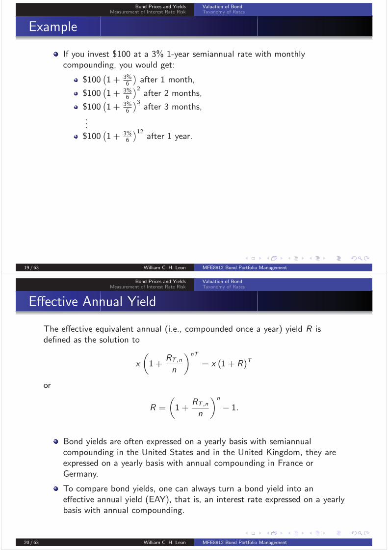
To apply present value formulas, one must have information about both thetime basis (usually interest rates are expressed on an annual basis) and thecompounding frequency.

Careful attention needs to be paid to the question of how an interest rate isdefined: An amount $x invested at the T -year interest rate RT ,n expressed onan annual basis and compounded n times per year grows to the amount

x

(1 +

RT ,n

n

)nT

after T years.




Example

If you invest $100 at a 6% 2-year annual rate with semiannualcompounding, you would get:

$100(1 + 6%

2

)after 6 months,

$100(1 + 6%

2

)2after 1 year,

$100(1 + 6%

2

)3after 1.5 year,

$100(1 + 6%

2

)4after 2 years.

If you invest $100 at a 4% 3-year semiannual rate with semiannualcompounding, you would get:

$100 (1 + 4%) after 6 months,$100 (1 + 4%)2 after 1 year,$100 (1 + 4%)3 after 1.5 year,...$100 (1 + 4%)6 after 3 years.




Example

If you invest $100 at a 3% 1-year semiannual rate with monthlycompounding, you would get:

$100(1 + 3%

6

)after 1 month,

$100(1 + 3%

6

)2after 2 months,

$100(1 + 3%

6

)3after 3 months,

...$100

(1 + 3%

6

)12after 1 year.




Effective Annual Yield

The effective equivalent annual (i.e., compounded once a year) yield R isdefined as the solution to

x

(1 +

RT ,n

n

)nT

= x (1 + R)T

or

R =

(1 +

RT ,n

n

)n

− 1.

Bond yields are often expressed on a yearly basis with semiannualcompounding in the United States and in the United Kingdom, they areexpressed on a yearly basis with annual compounding in France orGermany.

To compare bond yields, one can always turn a bond yield into aneffective annual yield (EAY), that is, an interest rate expressed on a yearlybasis with annual compounding.




Continuous Compounding

It seems desirable to have a homogeneous convention in terms of compoundingfrequency. This is where the concept of continuous compounding is useful.

Let the compounding frequency increase without bound,

limn→∞

x

(1 +

RT ,n

n

)nT

= x eRcT

where Rc expressed on an annual basis is a continuously compounded rate.

Note that

Rc = lim

n→∞

RT ,n = limn→∞

ln

(1 +

RT ,n

n

)n

.




Continuous Compounding: Proof

Since

ln

(1 +

RT ,n

n

)n

= n ln

(1 +

RT ,n

n

)= RT ,n

ln(1 +

RT,n

n

)− ln 1

RT,n

n

,

and limn→∞

RT,n

n= 0 and limy→0

ln(1+y)−ln 1y

= 1, we have

limn→∞

ln

(1 +

RT ,n

n

)n

= limn→∞

RT ,n = Rc .




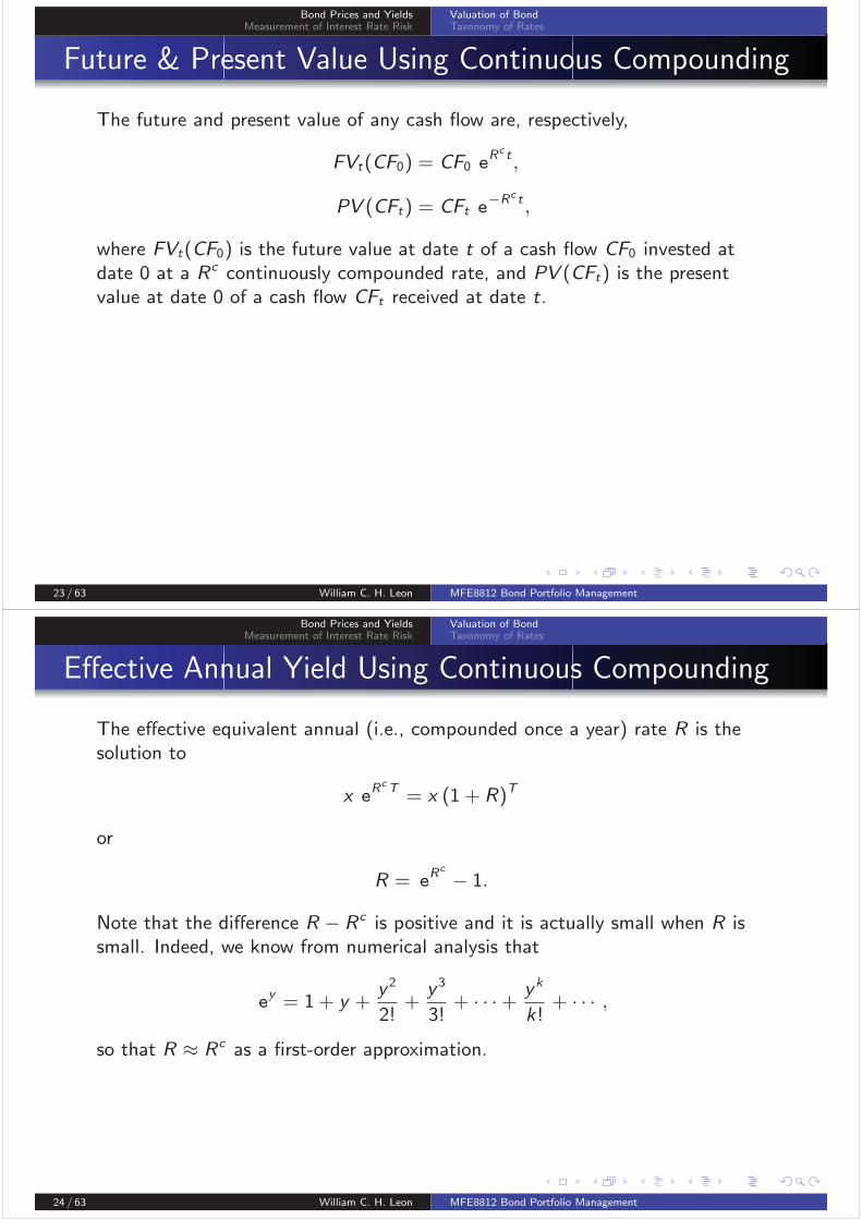
Future & Present Value Using Continuous Compounding

The future and present value of any cash flow are, respectively,

FVt(CF0) = CF0 eRc t ,

PV (CFt) = CFt e−Rc t ,

where FVt(CF0) is the future value at date t of a cash flow CF0 invested atdate 0 at a Rc continuously compounded rate, and PV (CFt) is the presentvalue at date 0 of a cash flow CFt received at date t.




Effective Annual Yield Using Continuous Compounding

The effective equivalent annual (i.e., compounded once a year) rate R is thesolution to

x eRcT = x (1 + R)T

or

R = eRc

− 1.

Note that the difference R − Rc is positive and it is actually small when R issmall. Indeed, we know from numerical analysis that

ey = 1 + y +

y 2

2!+

y 3

3!+ · · ·+

y k

k!+ · · · ,

so that R ≈ Rc as a first-order approximation.




Different Types of Rates & Yields

There are a host of types of interest rates involved in the fixed-income jargon.

Coupon rates.

Current yields.

Yields to maturity.

Spot zero-coupon rates.

Forward rates.




Coupon Rates

The coupon rate is the stated interest rate on a security, referred to as anannual percentage of face value.

It is called the coupon rate because bearer bonds carry coupons forinterest payments. Each coupon entitles the bearer to a payment when aset date has been reached. Today, most bonds are registered in holdersnames, and interest payments are sent to the registered holder, but theterm coupon rate is still widely used.

Coupon or interest payment is commonly made twice a year (in the UnitedStates, for example) or once a year (in France and Germany, for example).

The coupon rate is essentially used to obtain the cash flows and shall notbe confused with the current yield.




Current Yield

The current yield yc is obtained using the following formula

yc =c N

P,

where c is the coupon rate, N is the nominal value and P is the current price.

For example, a par $1,000 bond has an annual coupon rate of 7%, so itpays $70 a year.

If you buy the bond for $900, your actual current yield is

7.78% =$70

$900.

If you buy the bond for $1,100, your actual current yield is

6.36% =$70

$1, 100.




Yield to Maturity

The yield to maturity (YTM) is the single rate that sets the present value ofthe cash flows equal to the bond price, i.e., the YTM y solves the equation

T∑t=1

CFt(1 + y

)t = P,

where CFt is the cash flow at time t, T is the number of cash flows, and P isthe current price.




Yield to Maturity(Continue)

More precisely, the bond price P is found by discounting future cash flows backto their present value as indicated in the two following formulas depending onthe coupon frequency:

When coupons are paid annually,

P =

T∑t=1

CFt(1 + y

)t ,where the yield denoted by y is expressed on a yearly basis with annualcompounding, and T is the number of annual periods.

When coupons are paid semiannually,

P =

2T∑t=1

CFt(1 + y2

2

)t ,where the yield denoted by y2 is expressed on a yearly basis withsemiannual compounding, and 2T is the number of semiannual periods.




Exercise

Consider a $1,000 face value 3-year bond with 10% annual coupon, whichsells for 101. What is the yield to maturity of this bond?

Consider a $1,000 nominal value 2-year bond with 8% coupon paidsemiannually, which sells for 103–23 (i.e., 103 23

32). What is the yield to

maturity of this bond?




Answer




Yield to Maturity & Internal Rate of Return

The YTM is the internal rate of return (IRR) of the series of cash flows.Hence, each cash flow is discounted using the same rate. We implicitlyassume that the yield curve is flat at a point in time.

An IRR is an average discount rate assumed to be constant over thedifferent maturities. It is equivalently the unique rate that would prevail ifthe yield curve happened to be flat at date t (which of course is notgenerally the case). It is computed by trial and error, but may be easilydetermined by using built-in functions in financial calculators orspreadsheet softwares (e.g., the IRR function in Microsofts Excel).




Yield to Maturity as a Total Return Rate

A YTM may also be seen as a total return rate.

Consider a bond with a 3-year maturity and a YTM of 10% selling for$875.66. The bond pays an annual coupon of $50 and a principal of$1,000 at maturity.

If we buy the bond today, we will receive $50 at the end of the firstyear, $50 at the end of the second year and $1,050 after 3 years.Assuming that we reinvest the intermediate cash flows, i.e., thecoupons paid after 1 year and 2 years, at an annual rate of 10%.The total cash flows we receive at maturity are

$50× (1 + 10%)2 + $50× (1 + 10%) + $1, 050 = $1, 165.50.

Our investment therefore generates an annual total return rate y

over the period, such that

(1 + y)3 =1, 165.50

875.66=⇒ y = 10%.




Yield to Maturity & Price

Under certain technical conditions, there exits a one-to-onecorrespondence between the YTM and the price of a bond. Thus, giving aYTM for a bond is equivalent to giving a price for the bond. It should benoted that this is precisely what is actually done in the bond market,where bonds are often quoted in YTM, i.e., YTM is just a convenient wayof reexpressing bond price.

A bond YTM is not a very meaningful number. This is because there isno reason one should discount cash flows occurring on different dates witha unique discount rate. Unless the term structure of interest rates is flat,there is no reason one would consider the YTM on a T -year bond as therelevant discount rate for a T -year horizon. The relevant discount rate isthe T -year pure discount rate. In other words, YTM is a complex averageof pure discount rates that makes the present value of the bondspayments equal to its price.




Spot Zero-Coupon Rate

The spot zero-coupon rate R(0, t) is implicitly defined by

B(0, t) =1(

1 + R(0, t))t

where B(0, t) is the market price at date 0 of a bond paying off $1 at date t.

Note that such a bond may not exist in the market.

The yield to maturity and the zero-coupon rate of a strip bond (i.e., azero-coupon bond) are identical.

In practice, when we know the spot zero-coupon yield curve t �→ R(0, t),we are able to obtain spot prices for all fixed-income securities with knownfuture cash flows.

Zero-coupon rates make it possible to find other very useful forward ratesand par yields.




Forward Rate

If R(0, t) is the rate at which you can invest today in a t period bond, we candefine an implied forward rate (or forward zero-coupon rate) between years t1and t2 as

F (0, t1, t2 − t1) =

⎛⎜⎝

(1 + R(0, t2)

)t2

(1 + R(0, t1)

)t1

⎞⎟⎠

1t2−t1

− 1.

It is the forward rate as seen from date t = 0, starting at date t = t1, andwith residual maturity t2 − t1.

Basically, it is the rate at which you could sign a contract today to borrowor lend between periods t1 and t2.

In practice, it is very common to draw the forward curve τ �→ F (0, t, τ)with rates starting at date t.

Denote its continuously compounded equivalent as F c(0, t1, t2 − t1).




Forward Rate: A Rate That Can Be Guaranteed

The forward rate is the rate that can be guaranteed now on a transactionoccurring in the future.

Suppose we simultaneously borrow and lend $1 repayable at the end of 2years and 1 year, respectively. The cash flows generated by thistransaction are as follows:

Today In 1 Year In 2 Year

Borrow (2 Year) 1 −(1 + R(0, 2)

)2Lend (1 Year) −1 1 + R(0, 1)

Net Cash Flow 0 1 + R(0, 1) −(1 + R(0, 2)

)2This is equivalent to borrowing 1 + R(0, 1) in 1 year, repayable in 2 years

at the amount(1 + R(0, 2)

)2.




Forward Rate: A Rate That Can Be Guaranteed(Continue)

Borrowing 1 + R(0, 1) in 1 year and repaying(1 + R(0, 2)

)2in 2 years has

the implied rate on the loan given by(1 + R(0, 2)

)21 + R(0, 1)

− 1 = F (0, 1, 1).

Thus, F (0, 1, 1) is the rate that can be guaranteed now for a loan startingin 1 year and repayable after 2 years.




Spot Zero-Coupon Rate & Forward Rate

The spot zero-coupon rate R(0, ·) and forward rates F (0, ·, ·) are related asfollow:

R(0, t) =((

1 + R(0, 1))(1 + F (0, 1, 1)

)(1 + F (0, 2, 1)

). . .

. . .(1 + F (0, t − 1, 1)

)) 1t− 1

and

F (0, t1, t2− t1) =((

1+F (0, t1, 1))(1+F (0, t1+1, 1)

)(1+F (0, t1+2, 1)

). . .

. . .(1 + F (0, t2 − 1, 1)

)) 1t2−t1

− 1.




Forward Rate as a Break-Even Point

The forward rate may be considered as the break-even point that equalizes therates of return on bonds (which are homogeneous in terms of default risk)across the entire maturity spectrum.

Suppose that a zero-coupon yield curve today from which we derive theforward yield curve starting in 1 year is as follow:

Zero-coupon Rate Forward Rate Starting in 1 Year

R(0,1) 4.00% F(0,1,1) 5.002%

R(0,2) 4.50% F(0,1,2) 5.504%

R(0,3) 5.00% F(0,1,3) 5.670%

R(0,4) 5.25% F(0,1,4) 5.878%

R(0,5) 5.50%




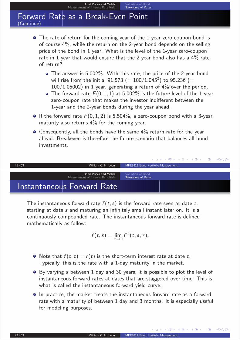
Forward Rate as a Break-Even Point(Continue)

The rate of return for the coming year of the 1-year zero-coupon bond isof course 4%, while the return on the 2-year bond depends on the sellingprice of the bond in 1 year. What is the level of the 1-year zero-couponrate in 1 year that would ensure that the 2-year bond also has a 4% rateof return?

The answer is 5.002%. With this rate, the price of the 2-year bondwill rise from the initial 91.573 (= 100/1.0452) to 95.236 (=100/1.05002) in 1 year, generating a return of 4% over the period.The forward rate F (0, 1, 1) at 5.002% is the future level of the 1-yearzero-coupon rate that makes the investor indifferent between the1-year and the 2-year bonds during the year ahead.

If the forward rate F (0, 1, 2) is 5.504%, a zero-coupon bond with a 3-yearmaturity also returns 4% for the coming year.

Consequently, all the bonds have the same 4% return rate for the yearahead. Breakeven is therefore the future scenario that balances all bondinvestments.




Instantaneous Forward Rate

The instantaneous forward rate f (t, s) is the forward rate seen at date t,starting at date s and maturing an infinitely small instant later on. It is acontinuously compounded rate. The instantaneous forward rate is definedmathematically as follow:

f (t, s) = limτ→0

Fc(t, s, τ).

Note that f (t, t) = r(t) is the short-term interest rate at date t.Typically, this is the rate with a 1-day maturity in the market.

By varying s between 1 day and 30 years, it is possible to plot the level ofinstantaneous forward rates at dates that are staggered over time. This iswhat is called the instantaneous forward yield curve.

In practice, the market treats the instantaneous forward rate as a forwardrate with a maturity of between 1 day and 3 months. It is especially usefulfor modeling purposes.




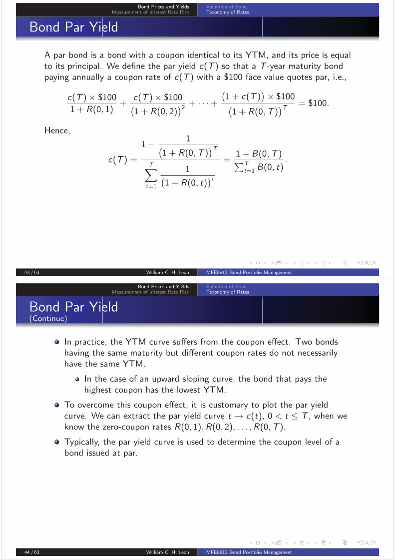
Bond Par Yield

A par bond is a bond with a coupon identical to its YTM, and its price is equalto its principal. We define the par yield c(T ) so that a T -year maturity bondpaying annually a coupon rate of c(T ) with a $100 face value quotes par, i.e.,

c(T )× $100

1 + R(0, 1)+

c(T )× $100(1 + R(0, 2)

)2 + · · ·+

(1 + c(T )

)× $100(

1 + R(0,T ))T = $100.

Hence,

c(T ) =

1−1(

1 + R(0,T ))T

T∑t=1

1(1 + R(0, t)

)t=

1− B(0,T )∑T

t=1 B(0, t).




Bond Par Yield(Continue)

In practice, the YTM curve suffers from the coupon effect. Two bondshaving the same maturity but different coupon rates do not necessarilyhave the same YTM.

In the case of an upward sloping curve, the bond that pays thehighest coupon has the lowest YTM.

To overcome this coupon effect, it is customary to plot the par yieldcurve. We can extract the par yield curve t �→ c(t), 0 < t ≤ T , when weknow the zero-coupon rates R(0, 1),R(0, 2), . . . ,R(0,T ).

Typically, the par yield curve is used to determine the coupon level of abond issued at par.



Full Valuation ApproachDuration & Convexity Approach

Overview

The value of a bond moves in the opposite direction to a change ininterest rates. If interest rates increase (decrease), the price of a bond willdecrease (increase).

A key to measuring the interest rate risk is the accuracy in estimating thevalue of the position after an adverse interest rate change. A valuationmodel determines the value of a position after an adverse interest ratemove. Consequently, if a reliable valuation model is not used, there is noway to properly measure interest rate risk exposure.

There are two approaches to measuring interest rate risk:

1 the full valuation approach, and2 the duration & convexity approach.




Full Valuation Approach

The full valuation approach approach requires the re-valuation of a bond orbond portfolio for a given interest rate change scenario.

The full valuation approach is a straightforward approach but can be verytime consuming.

If one has a good valuation model, assessing how the value of a bond willchange for different interest rate scenarios measures the interest rate riskof the bond.

This approach is sometimes referred to as scenario analysis because itinvolves assessing the exposure to interest rate change scenarios.




Example

Consider a $10 million par value position in a 20-year bond with 9% semiannualcoupon. The current price of the bond is 134.67216 with a yield to maturity of6%. The market value of the position is $13,467,216 (= 134.67216%× $10million). Suppose that yields change instantaneously for the following threescenarios:

1 50 basis point increase;

2 100 basis point increase; and

3 200 basis point increase.

The following table shows what will happen to the bond position if the yield onthe bond increases from 6% to (1) 6.5%, (2) 7%, and (3) 8%:

Yield New New New Percentage

Scenario Change (bp) Yield Price Value ($) Change

1 50 6.5% 127.76054 12,776,054 −5.13%

2 100 7.0% 121.35507 12,135,507 −9.89%

3 200 8.0% 109.89639 10,989,639 −18.40%




Full Valuation Approach(Continue)

A common question that often arises when using the full valuationapproach is which scenarios should be evaluated to assess interest rate riskexposure.

There may be specified scenarios established by regulators forregulated entities.

It is common for regulators of depository institutions to requireentities to determine the impact on the value of their bond portfoliofor a 100, 200, and 300 basis point instantaneous change in interestrates.

Risk managers tend to look at extreme scenarios to assess exposureto interest rate changes. This practice is referred to as stress testing.The state-of-the-art technology involves using a complex statisticalprocedure (such as principal component analysis) to determine alikely set of interest rate scenarios from historical data.

The full valuation approach can also handle scenarios where the yieldcurve does not change in a parallel fashion.




Duration

Duration is a measure of the approximate price sensitivity of a bond to interestrate changes. More specifically, duration of a bond, D, is the approximatepercentage change in price for a change in rates, i.e.

D = −ΔP/P

Δy=

P−− P+

2P Δy, (1)

where

P is the current price,

Δy is the change in the yield,

P− is the price when yield decreases by Δy , and

P+ is the price when yield increases by Δy .




Price-Yield Relationship for an Option-Free Bond







Duration(Continue)

Duration is the linear approximation of the percentage price change.

To improve the approximation provided by duration, an adjustmentfor “convexity” can be made. Combining duration with convexity toestimate the percentage price change of a bond caused by changes ininterest rates is called the duration & convexity approach.

Duration is interpreted as the approximate percentage change in price fora 100 basis point change in rates.

A common question asked about this interpretation of duration is theconsistency between the yield change that is used to computeduration using equation (1) and the interpretation of duration.Note that regardless of the yield change Δy used to estimateduration in equation (1), the interpretation is the same. i.e., if weused a 25 basis point change in yield to compute the prices used inthe numerator of equation (1), the resulting duration is stillinterpreted as the approximate percentage price change for a 100basis point change in yield.




Modified Duration & Effective Duration

Modified duration is the approximate percentage change in a bonds pricefor a 100 basis point change in yield assuming that the bonds expectedcash flows do not change when the yield changes.

This means that in calculating the values of P− and P+ for thevalue of duration, the same cash flows used to calculate P are used.Therefore, the change in the bonds price when the yield is changed isdue solely to discounting cash flows at the new yield level.

Effective duration is the approximate percentage change in a bonds pricefor a 100 basis point change in yield taking into account how the expectedcash flows may change when the yield changes.

Some valuation models for bonds with embedded options take intoaccount how changes in yield will affect the expected cash flows.Thus, when P− and P+ are the values produced from thesevaluation models, the resulting duration takes into account both thediscounting at different interest rates and how the expected cashflows may change.




Exercise

Consider a 20-years standard par bond with a 6% annual coupon.

What is the duration, assuming the yield increases or decreases 10 basispoints?




Answer




Application of Duration

To approximate the percentage price change, ΔP/P, for a given change inyield, Δy (in decimal), and a given duration, D, we may use the followingformula:

ΔP

P= −DΔy .

The negative sign on the right-hand side of the equation is due to theinverse relationship between price change and yield change (e.g., as yieldsincrease, bond prices decrease).




Exercise

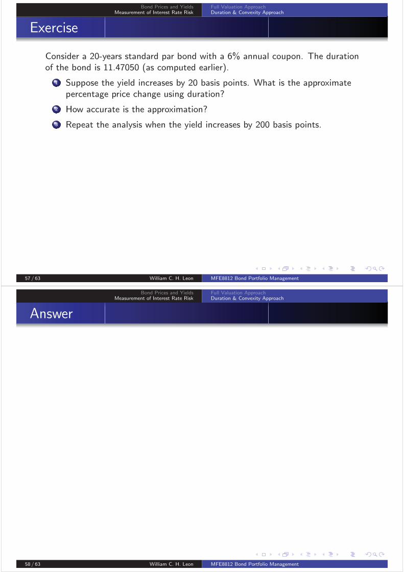
Consider a 20-years standard par bond with a 6% annual coupon. The durationof the bond is 11.47050 (as computed earlier).

1 Suppose the yield increases by 20 basis points. What is the approximatepercentage price change using duration?

2 How accurate is the approximation?

3 Repeat the analysis when the yield increases by 200 basis points.




Answer




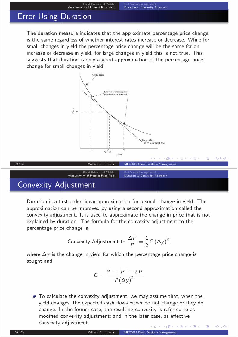
Error Using Duration

The duration measure indicates that the approximate percentage price changeis the same regardless of whether interest rates increase or decrease. While forsmall changes in yield the percentage price change will be the same for anincrease or decrease in yield, for large changes in yield this is not true. Thissuggests that duration is only a good approximation of the percentage pricechange for small changes in yield.




Convexity Adjustment

Duration is a first-order linear approximation for a small change in yield. Theapproximation can be improved by using a second approximation called theconvexity adjustment. It is used to approximate the change in price that is notexplained by duration. The formula for the convexity adjustment to thepercentage price change is

Convexity Adjustment toΔP

P=

1

2C(Δy

)2,

where Δy is the change in yield for which the percentage price change issought and

C =P− + P+

− 2P

P(Δy

)2 .

To calculate the convexity adjustment, we may assume that, when theyield changes, the expected cash flows either do not change or they dochange. In the former case, the resulting convexity is referred to asmodified convexity adjustment; and in the later case, as effectiveconvexity adjustment.




Duration & Convexity Adjustment

The following formula provides a better approximation of the percentage pricechange, ΔP/P, for a given change in yield, Δy (in decimal), and a givenduration, D, and convexity, C :

ΔP

P= −DΔy +

1

2C(Δy

)2.




Exercise

Consider a 20-years standard par bond with a 6% annual coupon. The durationof the bond is 11.47050 (as computed earlier).

1 Using a 10 basis points change in the yield, compute the convexity of thebond.

2 Suppose the yield increases by 200 basis points. What is the approximatepercentage price change using duration and convexity?

3 How accurate is the approximation?




Answer


MFE8812 Bond Portfolio Management - Nanyang …2p… · Bond Prices and Yields Measurement of...

Documents

Transcript of MFE8812 Bond Portfolio Management - Nanyang …2p… · Bond Prices and Yields Measurement of...