MFC and proportional valves - cms.esi.info

System Catalog 6

Solenoid valves I Process and control valves I Pneumatics

Sensors I MicroFluidics I MFC and proportional valves

The smart choice of Fluid Control Systems

All technical details were valid at the

time of going to print. Since we are

continuously developing our products,

we reserve the right to make technical

alterations. Unfortunately, we also

cannot fully exclude possible errors.

Please understand that no legal claims

can be made bared upon either the

details given or the illustrations and

descriptions provided.

Texts, photographs, technical draw-

ings and any other form of presenta-

tions made in this publication are pro-

tected by copyright and property of

Bürkert Fluid Control Systems GmbH

& Co. KG.

Any further use in print or electronic

media requires the express approval

of Bürkert GmbH & Co. KG. Any form

of duplication, translation, processing,

recording on microfilm or saving in

electronic systems is prohibited with-

out the express approval of

Bürkert GmbH & Co. KG.

Bürkert GmbH & Co. KG

Fluid Control Systems

Christian-Bürkert-Straße 13-17

D-74653 Ingelfingen

Contents

1. Principles of thermal mass flow measurement 1.1. Measuring gaseous substances Page 9

1.2. Explanation of the thermal (anemometric) measuring method Page 11

1.3. Calibration of thermal mass fLow meters Page 12

2. Basic design of mass flow controllers (MFC) and mass flow meters (MFM)

2.1. Description of the control loop Page 13

2.2. Characteristic parameters Page 13

3. Components of a mass flow controller/meter 3.1. Mass flow sensor Page 15

3.1.1. Inline sensor, direct measurement in the main flow Page 15

3.1.2. Bypass sensor, indirect measurement in the bypass flow Page 16

3.1.3. Bypass CMOS sensor, direct measurement in the bypass flow Page 17

3.2. Digital electronics Page 17

3.3. Proportional solenoid valve acting as final control element in a mass flow controller Page 17

4. Expanded functionality of Bürkert MFCs/MFMs4.1. Special hardware features Page 19

4.2. Mass Flow Communicator communication software Page 20

5. MFC/MFM range Page 21

6. Brief instructions: How to select the right Page 22MFC/MFM for an application

7. Bürkert MFC/MFM Type descriptions 7.1. MFC Type 8712, MFM Type 8702 Page 24

7.2. MFC Type 8710, MFM Type 8700 Page 25



8. Example applications 8.1. Industrial furnace control Page 28

8.2. Burner control Page 29

8.3. Bioreactor control Page 29

9. Proportional valves9.1. Features of solenoid-operated proportional valves Page 30

9.2. Actuating proportional valves Page 33

9.3. Characteristic parameters of proportional valves Page 34

9.4. Rating of proportional valves Page 35

9.5. Use of proportional valves in open and closed control loops Page 37

10. Proportional valve range 10.1. Brief instructions: How to find the right proportional valve? Page 40

10.2. Type selection diagrams Page 41

10.3. Overview of possible actuators Page 43

11. Type descriptions of proportional valves and actuators

11.1. Type 2821 Direct-acting 2/2-way Proportional Valve Page 44








11.9. Type 6024 Direct-acting 2/2-way Proportional Valve low-∆p Page 48

11.10. Type 6223 Servo-assisted 2/2-way high-flow Proportional Valve Page 48

11.11. Type 1094 Control electronics for proportional valves Page 49

11.12. Type 8623-2 Flow controller for proportional valves 0

11.13. Type 8624-2 Flow-pressure controller for proportional valves Page 50

11.14. Type 8625-2 Temperature controller for proportional valves Page 51

12. Application example Page 52

13. Conversion of various units Page 54

14. List of keywords Page 55

6/7

Digital right

from the start

Whether for use in the automotive or

aircraft sector, chemical or biotechno-

logy industries – mass flow controllers

from Bürkert are among the most in

demand for thermal mass flow measu-

rement due to their incomparable

accuracy and reproducibility. This

success is based on the fact that from

the very outset, MFCs were made

with future technology in mind, or to

be more precise, with digital technol-

ogy. The advantage of controlling all

the required processes via software

and the ability to save the relevant

data in the memory is still a major

feature in favor of the practical

system technology supplied from

the Ingelfingen based company.

Measured by the future

With their outstanding control proper-

ties, such as optimal dynamic and

digital control via serial interfaces or

field bus, Bürkert MFCs are ideal for

the applications of the future. But

even as we speak, the trend is moving

towards miniaturized semiconductor

sensors that are positioned in the ac-

tual gas flow. The latest sensor tech-

High tech for mass f low measurement

nology enables the achievement of

even faster and more sensitive meas-

urement results. Even measurements

in the main flow can become a matter

of course with Bürkert technology.

In short, our developers set the

standards for pioneering mass flow

technology.

Error diagnostics

included

The new generation of mass flow

controllers notify the operator if they

require servicing or are malfunction-

ing. While this is not a sensation,

of course, it simply demonstrates the

overall vision at Bürkert. Technical

“intelligence” in every sense of the

word is combined to form a system

that ensures that production process

can continue at all times. Maximum

economy is one of the main features

of the effective functioning of the me-

asurement and control systems, which

handle a whole range of flow measu-

rement volumes, from large

industrial furnaces to dosing 20 milli-

liters per hour. Technology that adds

up. A claim that we make for every

single component and every single sy-

stem.

When the going gets

tough

Mass flow controllers are components

that are responsible for ensuring the

precise control of gases even under

the harshest conditions (see our illu-

strated example). MFCs from Bürkert

are control instruments that reduce

the tolerances between individual

batches and therefore dramatically in-

crease the quality of the product. One

example of this is hardening materials

for which specific furnace atmospheres

are required. Among other things,

mass flow controllers control the ni-

trogen, ammonia, carbon dioxide

and air levels in the furnace chamber.

This means that gas consumption

can be controlled more accurately

than ever before. And moreover, new

processes, recipes and gas volumes

can be created in a particularly re-

producible form. The bottom line is

maximum quality in the process and

thus also in the end product.

8/9

Bürker t Mass F low Contro l lers | Meter

0

0 1,8 3

30 50

30

500

Mass flow meters (MFM) for gases

Type 8710

Type 8716

Type 8626

Type 8706

Type 8006

Type 8702

Type 8700

Type 8712

90

1500

m3N/h

Air

lN/min

0.02 – 50 lN/min

25 – 500 lN/min

25 – 1500 lN/min

25 – 1500 lN/min

25 – 1500 lN/min0.02 – 50 lN/min

0.05 – 30 lN/min

0.05 – 30 lN/min

Mass flow controllers (MFC) for gases

Range of possible measuring range limits using the example of Type 8712The instrument can be calibrated in the minimum case to a measuring range of 0.4 – 20 mlN/min or in the maximum case to 1 – 50 lN/min, each relating to using air as the medium.

1.1.Measuring gaseoussubstances

In contrast to liquids, gases can becompressed. The gas density changesdepending on the pressure and temperature. Pursuant to the idealstatus equation for gases

the volume in the example in Figure 1changes from 1 m3 upstream of thecompressor to 0.172 m3 downstreamof the compressor. Since there is a flow in the example, the volume isspecified dependent on the time (volume flow).

The transported quantity of substanceis independent of the pressure andtemperature.The figure shows the air mass flow.This remains constant at 1.205 kg/hover the entire distance. The densitychanges from 1.205 kg/m3 upstream of the compressor to

downstream of the compressor. Thegas volumes can only be compared if they relate to the same conditions.In general the mass flow is specifiedas a standard volume flow, in otherwords, in the form of a volume flow as defined in DIN 1343.

,

1. Pr inc ip les of thermal mass f low measurement

Figure 1: Diagram of volume flow change, depending on the measurementposition

=p1 · V1

T1

p2 · V2

T2

· ·= =V2 = 0.172 m3p1 · V1

T1

T2

p2

1 bar · 1 m3

293K

353K7 bar

= = 7.0012 =mV2

1.205 kg0.172 m3

kgm3

Inlet air

Volume flow 1 m3/h 0.172 m3/h 0.167 m3/hTemperature 20 °C (293 K) 80 °C (353 K) 20 °C Pressure 1 bar(a) 7 bar(a) 6 bar(a) Density 1.205 kg/m3 7.001 kg/m3 7.23 kg/m3

Mass flow 1.205 kg/h 1.205 kg/h 1.205 kg/h

Load—Meter 1

Compressor Long pipe run

Meter 2 Meter 3

�

10/11

The conventional measuring methods for measuring gas volumes are

■ Floats (rota meters):In practice, floats do not perform their measurement either in the volume flow or in the mass flow. They can be used for gases or fluids with a low pressure loss. The measuring span is approx. 10:1. If floats are operated in calibrated conditions, they supply the mass flow.

■ Orifices:With orifices, the gas quantity is obtained by deriving it from the pressure differential. To obtain the mass flow, it must be ensured that the pressure and temperature re-main constant at the measurement point. The measuring span is the same as for floats.

■ Vortex:Vortex sensors measure the volumeflow that then has to be converted into the mass flow. They have a very linear characteristic curve and are suitable for contaminated media.Special attention must be paid to the design of the input and output sections for this measuring method.

■ Coriolis:Sensors of this type measure the mass flow itself. They do not need any input and output sections and can also measure fluids. The meas-uring method and the sophisticated electronics are reflected in the price.

■ Anemometers(thermal measurement):Anemometers measure the mass flow itself, independent of the pressure and temperature, and offera good measuring span of greateror equal to 50:1. Depending on the design of the sensor, they canalso be used to measure fluids.

Bürkert Mass Flow Controllers and Meters (MFCs and MFMs) use the anemometric principle: measurement signals can be easily evaluated and the measur-ing method is very sensitive to slight flow-rate changes.

Table 1: Principles of thermal mass flow measurement

Measured variable Definition Typ. units RemarksVolume flow Q Gas volume flow The most common (operating flow rate) per unit of time l/min flow rateMass flow m Gas volume flow Measured variable relevant

per unit of time kg/h, g/s for most applications,Normal volume flow Gas volume flow a compromise between conventional QN=m/ N per unit of time, and relevant measured variable, (DIN 1343) converted into its volume in gas type-specific mass flow

standard conditions (T=0 °C/273K relating to the defined referenceand p=1013 mbar/760 Torr) lN/min, mN

3/h conditions. Standard volume flow Gas volume flow QS=m/ S per unit of time, converted

into its volume instandard conditions (T=20 °C/ lS/min, slpm,293K and p=1013 mbar/760 Torr) mS

3/h, sccm

.

.

.

�

�

1.2. Explanation of thethermal (anemometric)measuring method

The measured value pick-ups for thethermal measuring method are electri-cal resistors and part of a measure-ment bridge circuit (Figure 2). Theymay be in the actual flow channel (inline instrument) or wound aroundthe flow channel (bypass instrument).

The controller in Figure 2 sets thecurrent I so that the temperature dif-ferential between the heating resistorRS and the measuring resistor RT iskept constant at all times. Since RT

is very high ohm compared to RS, thecurrent IS is almost identical to currentI. The resistor RS is always heated tosuch a degree that there is always acertain overtemperature to the fluidtemperature, measured with RT. If gas flows past RS, heat is dissipatedmore or less effectively depending onthe gas. The heating current that is required to maintain the overtempera-ture is a function of the gas flow pass-ing through the channel and repre-sents the primary measured variable.The method is known as the CTA,Constant Temperature Anemometer,and is a variant of the thermal measu-ring method. Mass flow controllers/meters are designed as main flow orbypass flow instruments.

Figure 3 shows the measuring ele-ment of an inline instrument. The flow conditioning produces a uniformflow through the channel cross-sec-tion on the inline instrument. Inputsections to smooth the flow are there-fore not necessary.

Figure 2: Simplified electrical diagram of the measurement bridge circuit(resistors placed directly in the flow channel)

Bypass capillary

Laminar flow element

Main channel

RT RS

Flow

Temperature

No flow

Flow

L/2Pipe length

∆T

0 L

RT RS

T0

T1

Figure 4: Sketch of a bypass sensor block

Im

Controller

R T R S

I S

R K

R 2 R 1

Figure 3: Cross section of a main flow sensor block

Sensor electronics

Flow conditioning and upstream filter

Resistor RT (platinumlayer measuring resistorin thin-layer technology)

Supporting element

Resistor RS (platinumlayer measuring resistorin thin-layer technology)

.

12/13

Bypass flow or bypass sensors (seeFigure 4) essentially have a bypasscapillary around which the measuringresistors RT and RS are wrapped, aswell as a laminar flow element. The laminar flow element generates a pressure drop proportionate to theflow, which drives the flow throughthe bypass capillary. The element mustbe designed so that both the flow inthe bypass and in the main channel islaminar and that the proportions re-main constant.

Depending on the gas flow, the tem-perature conditions registered by themeasuring resistors change. Differenttechnical designs for the bypass principle are possible. The thermalmeasurement is based on the thermal properties of the gas, the geometricdesign of the measuring body and theflow velocity of the gas. In thermalterms, gases differ by their specificheat capacity cp and heat conductivity�F. This means that, depending on themeasured gas, the measuring range ofa unit can be greater or smaller.

1.3. Calibration of thermal mass flowmeters

In the calibration process, the measu-rement signal range of the sensor isclearly assigned to the flow control ormeasuring range. For this purpose,flow rates are set and the relevantsensor signals recorded on the basisof highly accurate flow normals (forexample, heating wire anemometers,which are regularly tested on a testbench with super-critical nozzles thathas been approved by the calibrationauthority). When the flow characteri-stic curve has been registered, theelectrical inputs and outputs can becalibrated. All the data are saved indigital form in an EEPROM. Mass flowcontrollers or meters generally containa calibration curve for a certain gas.They can only be used to control ormeasure a different gas if a secondcalibration curve has been stored. Exceptions to this rule are gases withvery similar properties (e.g. oxygenand nitrogen). In this case, a singleconversion factor is sufficient for theentire flow range. In principle, everygas mixture can be measured, provi-ded its composition does not change.

Mass flow controllers or meters areoften calibrated for the following gases:■ Air, nitrogen, oxygen and nitrous

oxide (laughing gas)■ Argon, helium, neon, krypton

(inert gases)■ Hydrogen, methane (natural gas),

ethylene, propane, butane■ Ammonia, carbon dioxide, carbon

monoxide, sulfur dioxide■ Mixtures of nitrogen and hydrogen

or methane, endogas, exogas, city gas, mixtures of methane andcarbon dioxide.

Figure 5: Calibration protocol

which enables a reproducible flowprofile at the site of the sensor andtherefore precise calibration. Long input and output sections to smooththe flow, such as those required forsensors bolted into pipelines are notnecessary. All MFCs and MFMs alsocontain input filters that can be re-placed easily without damaging anyother components.

2.2.Characteristic parameters

■ Full scale value range/Nominal flow rateThe full scale (F.S.) value range isthe range of possible measuringrange limits. The minimum value isthe smallest possible full scale val-ue for the nominal flow rate whilethe maximum value is the highestpossible full scale value for the nominal flow rate. Any full scale values between these are also pos-sible of course. The specificationsrefer to defined reference condi-tions (for example, standard litersper minute or standard cubic centi-meters per minute).

■ Operating medium/calibrationmediumThe operating medium is generallyused for the calibration process, although a reference gas (for example nitrogen) may be used in exceptional cases.

with the registeed control deviation(xd). The frequency of the PWM signalis tailored to the proportional valveused. In addition, the actual value isoutput by an analog electrical interfaceor a field bus (xout) and is available tothe user for control purposes or forfurther evaluation (for example toestablish consumption by integration).The mass flow meter has the samecomponents as the MFC with the exception of the proportional valve acting as a positioning valve, thus these instruments can only be used tomeasure mass flow, not to control it.The compact and integrated con-struction of mass flow controllers andmass flow meters ensures easy in-stallation and operation of the entireclosed-loop flow-rate control or mea-surement system. Additional worksuch as wiring and tuning individualcomponents or taking into accountpipe lengths is not necessary. The instruments supply very high-qualitymeasurement results. One of the reasons for this is that a great deal ofattention has been put into flow tech-nology. Inline instruments have a flowconditioning system at the input side,

xd = w – x

x

xout

w

p

y2

Q sensor Proportional valve

Controller

Figure 6: Components of a mass flow controller

2.1.Description of the control loop

Type 8626, 8716, 8712 and 8710mass flow controllers are compact instruments designed to control themass flow of gases. They maintain aspecified flow-rate set-point regard-less of disturbance variables such aspressure fluctuations or flow resi-stance that differs over time, for exam-ple as a result of filter contamination.MFCs contain a flow sensor (Q sen-sor), electronics (with signal process-ing, control and valve actuation func-tions) and a proportional solenoidvalve acting as the final control ele-ment or actuator (see Figure 6).

The set-point value (w) is defined byelectrical means using a standard sig-nal or field bus. The actual value (x)recorded by the sensor is comparedto the set-point value in the controller.A pulse width modulated voltage sig-nal is supplied to the proportional valveby the controller to act as the controlvariable (y2). The duty cycle of the voltage signal is varied in accordance

2. Basic design of mass f low contro l lers (MFC) andmass f low meters (MFM)

14/15

■ AccuracyThe most realistic is a combined figure in ± x % of rate ± y % of full scale value.

■ RepeatabilityFigure in ± x % of full scale value. Repeatability, or reproducibilityas it is also called, is a measure of the distribution of the actual valuesthat result from the repeated ad-justment of a reproduced set-point value, starting from a specific start-ing value.

■ LinearityFigure in ± x % of full scale value. Maximum deviation of the signaled actual value from the set-point val-ue, if this is passed slowly over the entire range.

■ SensitivityFigure in ± x % of full scale value. The smallest change in set-point value that results in a reproducible change in the flow rate.

■ SpanSpecified as a ratio, for example 1:50. Ratio of the smallest flow rate that can be adjusted to the nominal flow rate.

■ Settling timeTime required by the MFC to achieve 95 % of the difference between the old and new flow rate.

■ Response timeTime required by a MFM to adjust its display to 95 % of the new value after a sudden change in flow rate from Q1 to Q2.

=QMFM (t95)

Q1 + 0.95 (Q2 - Q1)

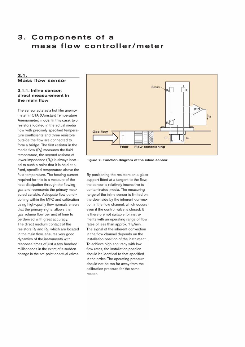
3.1. Mass flow sensor

3.1.1. Inline sensor, direct measurement in the main flow

The sensor acts as a hot film anemo-meter in CTA (Constant TemperatureAnemometer) mode. In this case, tworesistors located in the actual mediaflow with precisely specified tempera-ture coefficients and three resistorsoutside the flow are connected toform a bridge. The first resistor in themedia flow (RT) measures the fluidtemperature, the second resistor oflower impedance (RS) is always heat-ed to such a point that it is held at afixed, specified temperature above thefluid temperature. The heating currentrequired for this is a measure of theheat dissipation through the flowinggas and represents the primary mea-sured variable. Adequate flow condi-tioning within the MFC and calibrationusing high-quality flow normals ensurethat the primary signal allows the gas volume flow per unit of time to be derived with great accuracy.The direct medium contact of the resistors RT and RS, which are locatedin the main flow, ensures very gooddynamics of the instruments with response times of just a few hundredmilliseconds in the event of a suddenchange in the set-point or actual valves.

3. Components of a mass f low contro l ler/meter

By positioning the resistors on a glasssupport fitted at a tangent to the flow,the sensor is relatively insensitive tocontaminated media. The measuringrange of the inline sensor is limited onthe downside by the inherent convec-tion in the flow channel, which occurseven if the control valve is closed. It is therefore not suitable for instru-ments with an operating range of flowrates of less than approx. 1 lN/min.The signal of the inherent convectionin the flow channel depends on the installation position of the instrument.To achieve high accuracy with lowflow rates, the installation positionshould be identical to that specified in the order. The operating pressureshould not be too far away from thecalibration pressure for the same reason.

Sensor

RT RS

Flow conditioningFilter

Gas flow

RK

R1R2

IS

PID

Figure 7: Function diagram of the inline sensor

16/17

3.1.2. Bypass sensor, indirect measurement in the bypass flow

In this case, the measurement is takenusing the bypass principle. A laminarflow element in the main channel ge-nerates a slight pressure drop, whichdrives a small proportion of the fullflow through the actual sensor tube.Two heating resistors are wound onthin stainless steel tubes and areinterconnected to form a measurementbridge. When the medium passesthrough the tube, heat is transportedin the direction of the flow and thismisaligns the previously balancedbridge.The dynamics of the measurement isdetermined by the wall of the sensortube that acts as a thermal barrier andis therefore considerably poorer thanthat offered by sensors with resistorsdirectly in the medium flow, simply byvirtue of the principle employed. Using software algorithmus settling times are achieved which are ade-quate for the majority of applications(generally a few seconds).These sensors can also be used tocontrol some aggressive gases, sinceall the main parts that come into contact with the medium are made of stainless steel.

IBr

R1 R2

Sensor tube

Filter Laminar flow element

Gas flow P1 P2

Figure 8: Function diagram of the bypass measuring principle

3.1.3. Bypass CMOSsensor, direct measure-ment in the bypass flow

The measurement is taken directly inthe bypass channel. A laminar flowelement in the main channel generatesa slight pressure drop, which drives a small proportion of the full flowthrough the bypass channel. The sen-sor located therein records the massflow rate directly by measuring thetemperature differential. The measure-ment in this case is taken in a speciallyshaped flow channel whose wallscontain a Si chip in one place with an exposed diaphragm. Using CMO-Sens® technology, a heating resistoris connected to this diaphragm alongwith two temperature sensors up-stream and downstream of it.If the heating resistor is supplied witha constant voltage, the voltage differ-ential of the temperature sensors is a measure of the mass flow of the gas flowing through the flow channelpast the chip.

The low thermal mass of the tempera-ture sensors and their direct contactwith the flow (apart from a protectivelayer) means the sensor signal reactsextremely fast to quick flow-rate chan-ges and the MFC is capable of sett-ling set-point value or actual valuechanges within a few hundred milli-seconds. In addition, they are extre-mely sensitive, even with very low flow rates, and also offer additionalcorrection and diagnostic facilities viathe signal of a separate temperaturesensor located on the chip.

3.2. Digital electronics

Microprocessor electronics is used toprocess the current set-points andactual flow rates and actuate the finalcontrol element (proportional valve).The analog sensor signal is filtered bythe control electronics and convertedinto a value that corresponds to theactual flow rate using a calibrationcurve stored in the instrument. Thecontrol deviation xd between the set-point value w and the actual value x isprocessed by the controller using a PIalgorithm and is used to calculate themanipulated variable y2, with whichthe control valve is actuated. The control parameters are set during thecalibration process. To allow for theproperties of the controlled system,the controller uses system-dependentamplification factors that are detectedautomatically using a self-optimizationroutine (autotune). An overshoot (seeFigure 10) must be accepted for highdynamic requirements. The control dynamics can, however, be adjustedretrospectively using the Mass FlowCommunicator communication soft-ware. This also applies to the filter level and the smoothing of the actualvalue signal, which is returned. Figure10 shows the step response of massflow controller Type 8712 (withCMOS sensor), Figure 11 shows thesame from the mass flow controllerType 8626 (with inline sensor). The figures show the responses of the actual value and controller output signals when the set-point value is increased from 10 % to 95 %. Depending on the design of the in-strument, the set-point and actual value signals can be specified and returned in analog form via the stand-ard signal interface or in digital formvia an RS-232 or field bus interface.

Gas flow

Sensor element Heater T sensors

Figure 9: Function diagram of the bypass sensor in CMOSens® technology(cross section from the bypass channel)

18/19

Communication with the Mass FlowCommunicator software (see Section 4for further information) is via the RS-232 or RS-485 (depending on the instrument).In addition to reduced drift and offsetby the components, microprocessor-based digital electronics offer the majoradvantage that all the required pro-cesses can be controlled by software(flash-programmed, in other words, theelectronics can be updated). Data rele-vant to this (calibration curves, correc-tion functions, control functions, etc.)can be stored in the memory.

3.3. Proportional solenoidvalve acting as finalcontrol element in amass flow controller

Direct-acting plunger-type proportionalvalves (see Section 9, Proportionalvalves) from the Bürkert valve rangeare used as final control elements inall MFC series. Constructive measures,in particular on valves in the MFCs forlow flow rates (Types 8710 and 8712),ensure that the moving plunger is guided with low friction. Together withthe PWM actuation, this ensures aconstant, almost linear characteristiccurve along with high response sen-sitivity. Both of these features are important for optimal function in theMFC’s closed control loop. The nomi-nal diameters of the valves result fromthe required nominal flow rate Qnom,the pressure conditions in the appli-cation and the density of the operat-ing gas. Using these data, a propor-tional valve can be selected whoseflow-rate coefficient kVs allows the maximum flow of at least the requirednominal flow rate in the specifiedpressure conditions and in compliancewith the flow-rate equations:

The “valve authority” is important forthe MFC control properties in the sy-stem. It should not be below a valueof 0.3 ... 0.5.

Meaning of formula symbols:

kVa Flow-rate coefficient of sy-stem without installed MFCin m3/h

kVs Flow-rate coefficient of theMFC with final control ele-ment fully open in m3/h

(�p)0 Pressure drop through theentire system

(�p)V0 Proportion of this that dropsthrough the MFC with thevalve fully open.

The system section should not be designed in terms of its flow-ratecoefficient kVa, so that at the requirednominal flow rate, the vast majority ofthe available pressure is used thereand thus the selected nominal valvediameter is too large. In this case, thevalve authority is too small, in otherwords, only a small proportion of thevalve working range is used. This con-siderably impairs the resolution andcontrol quality of the MFC. If the sy-stem section is designed to be too“small”, increasing the nominal valvediameter will not help, and the remedyis either to increase the supply pres-sure or increase the kVa value, e.g. bymeans of a larger pipe diameter.

Time [s]

w, x, y2 [%]

010

0 0,2 0,4 0,6 0,8 1,0

20304050

Controller output signal y2

Actual value x

Set-point value w

60708090

100

Figure 10: Step response of Type8712 Mass Flow Controller after aset-point step from 10 % to 95 %

Time [s]

w, x, y2 [%]

01020304050

Controller output signal y2

Actual value x

Set-point value w

60708090

100

0 0,2 0,4 0,6 0,8 1,0

Figure 11: Step response of Type8626 Mass Flow Controller after aset-point step from 10 % to 95 %

� = = (∆p)V0

(∆p)0

kVs2

[kVa2 + kVs

2]

4.1. Special hardware features

■ All standard signals in analog form are available for the input ofthe set-point value or output of the actual value.Communication in digital form isenabled via the RS-232/RS-485 or field bus (e.g. Profibus DP orDeviceNet).

■ Digital microprocessor electronicsallow two gas calibrations in a single instrument (under the condition that the application parameters of the two gases canbe covered with the same rating).

■ Display of the operating status of the instrument using LEDPOWER-LED: The unit is readyCOMMUNICATION-LED: The instrument is communicating viafield bus or serial interfaceLIMIT (y)-LED: The instrument hasreached the settling or measuringlimitERROR-LED: Error display

■ 3 binary inputs (on Type8710/8700, 2 binary inputs)A fixed function can be assigned to the binary inputs, which is thenexecuted when the input is set. The following functions may be assigned (Table 2):

■ No additional shut-off valve is re-quired on the MFC since the finalcontrol element (proportional valve)performs the tight-closing function.

■ 2 relay outputs (on Type8710/8700, 1 relay output) takethe form of voltage-free SPDT contacts. Fixed events can be assigned to the relay outputs. If the event occurs, the output is set.The following assignments arepossible, for example (Table 3):

4. Expanded funct ional i ty o f Bürker tMFCs/MFMs

Table 2: without function No function is assigned to the binary input.

activate autotune The MFC goes into autotune mode in which the parameters dependent on the controlled system are optimized.

activate gas 2 This binary input allows the system to switch to gas 2 if the instrument has been calibrated for 2 gases.

safety value active If the binary input is set, the MFC settles on the flow rate set in the safety value, regardless of the set-point value.

reset totalizer The totalizer value is set to zero.safety value inactive Inverse action like a “safety value active”

(safety value is settled if the binary input is not set).

start predefined The pre-adjusted set-point profile is run.profilecontrol mode active The controller is no longer in control mode.

The valve pulse duty factor 0 ... 100 % is controlled by set-point figures 0 ... 100 %.

close valve The valve is closed regardless of the completely set-point value.open valve The valve is fully opened regardless of the completely set-point value.

Table 3:Power ON Voltage supply is connected to the unitAutotune active Autotune mode activeLimit Value has moved above or below the set limit value (e.g. for

actual value, set-point value, control signal or totalizer) Error Error has occurred (e.g. sensor break)

20/21

4.2. Mass Flow Communi-cator communicationsoftware

■ Customers can configure and pa-rameterize the instrument using theMass Flow Communicator PC soft-ware via the RS-232, e.g. configu-ration of binary inputs and outputs,LEDs, limit values, etc.

■ Limit value switches (limits) for set-point/actual value, control signaland integrated totalizer can be configured.

■ The dynamics of the instrumentcan be adjusted to the application.

■ Instrument behavior can be definedin the event of an error, for example:go to safety value, fully open orclose valve.

■ Autotune function: automatic adjustment of the controller to the system conditions.

■ Adjustable ramp function for theset-point value can be configured.

■ Set-point profile can be definedand stored. Set-point values withthe relevant time intervals can beentered in the required order inwhich the instrument automaticallymoves to them at a later time (forexample, after activating a binaryinput).

The latest version of the configurationsoftware can be downloaded from theBürkert website (www.buerkert.com).

5. MFC/MFM range

0.05–30 Bypass 10 VA 2821 2 1 Standard signal,(standard) 1.4305 2822 RS-232

0.02–50 Bypass 10 VA 2821 3 2 Standard(CMOS) 1.4305 2822 signal, RS-232

or fieldbus

25–1500 Inline 10 VA 6022 3 2 Standard 1.4305, 2834 signal, RS-232 Al 6024 or field busanod. 2836

8706:25–1500 Inline 10 VA 6022 3 2 Standard 8716: 1.4305, 2834 signal, RS-232 25–500 Al 6024 or field bus

anod.

Nom

inal

flow

rat

es

[l N/m

in]

(air

or N

2)

Mea

surin

gpr

inci

ple

Max

. ope

ratin

g pr

essu

re [b

ar]

Bod

y m

ater

ial

Pro

port

iona

l val

ves

(n

ot in

MFM

)

Bin

ary

inpu

ts

Bin

ary

outp

uts

Com

mun

icat

ion

Table 4: Overview of Bürkert Mass Flow Controllers/Meters

MFM type MFC type

8700 8710

8702 8712

8006 8626

8706 8716

22/23

Do you want to control/dose the gasor just measure it?

Mass flow controllers contain a pro-portional control valve that sets therequired gas throughput. Mass flowmeters only return the current gasthroughput in the form of an actual value signal.

What medium do you want to control or measure?

A mass flow controller/mass flow meter is calibrated for the operatinggas. If the operating gas is a mixture,the precise composition in percen-tages is important for the rating and calibration of the instrument. The relative humidity of the gas can be almost 100 %, but a liquid phasemust be avoided under all circum-stances. Particle contents should be removed by upstream filters. The medium resistance of wettedMFC/MFM components must be ensured. As a result of the gas properties, it may be necessary to carry out the calibration with the operating medium. For example, this will guarantee the reproducibility and accuracy of the instrument.

What process data are available?

To achieve the optimal design, in ad-dition to the required maximum flowrate Qnom, the pressure values imme-diately upstream and downstream of the MFC (p1, p2) at this flow rate Qnom

must be known. These often differfrom the input and output pressure ofthe system as a whole because bothupstream and downstream of theMFC, there may be additional flow resistors (pipes, shut-off valves, nozz-les, etc.). If the input pressure (p1)and output pressure (p2) are notknown or cannot be obtained by mea-surement, an estimate must be made,taking into account the approximatepressure drops through the flow resis-tors upstream and downstream of theMFC at Qnom. For rating purposes, it is also necessary to provide details of the medium temperature T1 and thestandard density �N of the medium(can be obtained for mixtures usingthe percentage values).

The possible measuring span must be checked to determine whether the minimum flow rate Qmin can be adjusted.The maximum expected input pressurep1max must be specified to ensure the tight-closing function of the final control element in the MFC under all operating conditions.

How can the MFC/MFM be connected to the pipes?

As a standard feature, the instrumentsare mounted using the screw-in threadto match the flow rate. However, in-struments can also be supplied withscrew-in connectors. The external dia-meter with a metric (mm) or imperial(inch) figure is important for the sizeof the screw-in connectors.

6. Br ie f inst ruct ions: How to se lect the r ight MFC/MFM for an appl icat ion

In what form is theset-point value setand the actual valuereturned?

The control electronics is digital. The interfaces may be either analog or digital. For analog transfer, it is possible toselect from the range of conventionalstandard signals, for digital commu-nication you can choose between RS-232 or RS-485 and field bus.

For information about all the relevantdesign data, please refer to the speci-fication sheet on the last page of thedata sheet.

Figure 12: Specification sheetThis enables you to benefit from the experience of Bürkert engineers in the planning phase of your system.

Figure 13: ConfiguratorThe data on the specification sheet are evaluated using the Bürkert MFC/MFM configurator. This tool aids Bürkert engineers in selecting the correct instrument on-site.

MFC application MFM application Quantity Required delivery date

Medium data Type of gas (or gas proportion for gas mixtures)Density [kg/m3]Media temperature [°C]

Fluidic data

Maximum flow Qnom lN/min 1) cmN

3/min 1)

mN3/h 1)

cmS3/min (sccm) 2)

kg/h lS/min (slpm) 2)

Minimum flow Qmin, lN/min 1) cmN

3/min 1)

mN3/h 1)

cmS3/min (sccm) 2)

kg/h lS/min (slpm) 2)

Pressure conditions Inlet pressure p1 [bar] Outlet pressure p2 [bar]Max. inlet pressure p1 [bar]Pipe run (outer-Ø) metric [mm] imperial [inch]MFC/MFM port connection without screw-in fitting G-thread (DIN ISO 228/1) NPT-thread (ANSI B1.2) with screw-in fittingMFC/MFM installation horizontal vertical, flow upwards vertical, flow downwards

Ambient temperature °C

Material data Body material Aluminum, anodised Stainless steelSeal material FPM Viton EPDM other:

Electrical data

Output/input signal 0-20 mA / 0-20 mA 4-20 mA /4-20 mA 0-10 V / 0-10 V 0-5 V / 0 - 5 VFieldbus communication Profibus-DP DeviceNet

How can we contact you?

Company Department

Contact person

Street Telephone/Fax

Postcode/Town E-Mail

Please copy, fill out and send to your nearest Burkert facility – you will find a Burkert address list on p. 372 of this catalogue

Specification sheet for MFC/MFM applications

operating at Qnom

1) at 1.013 bar (a) and 0°C 2) at 1.013 bar (a) and 20°C

24/25

7.1. MFC Type 8712, MFM Type 8702

The Type 8712 Mass Flow Controller and Type 8702 Mass Flow Meter arecharacterized by their new semiconductor flow sensors featuring CMOStechnology. This revolutionary bypass measuring technology enables attaining measurement and display times of a few hundred milliseconds.

Typical applications include■ Process engineering■ Packaging and food industries■ Environmental engineering■ Surface treatment■ Material coating■ Burner control systems■ Fuel cell technology

Characteristics:■ High level of accuracy■ Fast response and settling time■ Excellent span■ Optional calibration for two gases■ Integrated totalizer■ Field bus optional■ Mass Flow Communicator

(PC configuration software)■ 3 binary inputs and 2 binary

outputs (relay outputs)■ Galvanic isolation of inputs

and outputs

Main technical data:■ Full scale range 0.02 – 50 lN/min

(N2 at 273.15 K and 1013.25 mbar)

■ Settling time < 300ms■ Accuracy ± 0.8 % of rate ± 0.3 %

F.S. ■ Repeatability ± 0.1 % F.S. ■ Linearity ± 0.1 % F.S.■ Span 1:50, 1:500 on request■ Max. operating pressure 10 bar

depending on the application■ Type of protection IP 65■ Port connection G1/4, NPT1/4,

screw-in connector■ Analog signal transmission or

digital communication (RS-232,RS-485, field bus)

■ Voltage supply 24 V DC■ Power consumption max. 10 W■ Dimensions 115 x 137.5 x 37 mm■ Stainless steel body

7. Bürker t MFC/MFM type descr ip t ions

Figure 15: Electrical interfaces Type 8712/8702

(* Not with MFM)

15-pin socket

8-pin socket

Internal

External

9-pin socket

Actual value (analog)

Binary output 1 and 2 (NC or NO)PWM signal *(valve actuation)

LED display 1-4

Set-point value (analog) *and binary inputs 1-3

Sensor signal

Mass Flow controller(MFC)

Mass Flow Meter(MFM)

Input

Digital communicationI/O

Output

Serial interface (RS-232)

Field bus (PROFIBUSDP or DeviceNet)

Figure 14: MFC 8712, MFM 8702

Voltage supply

Figure 16: MFC 8710, MFM 8700

Typical applications include■ Process engineering■ Packaging and food industries■ Environmental engineering■ Surface treatment■ Material coating

Characteristics:■ High level of accuracy■ Excellent span■ Calibration of critical gases

with air and conversion factor■ Optional calibration for two gases■ Integrated totalizer■ Mass Flow Communicator


output (relay output)

Main technical data:■ Full scale range 0.05 –30 lN/min

(N2 at 273,15K and 1013.25 mbar)■ Settling time approx. 3 seconds■ Accuracy ±1.0 % of rate ± 0.3 %

F.S. ■ Repeatability ±0.2 % F.S. ■ Linearity ±0.25 % F.S.■ Span 1:50■ Max. operating pressure 10 bar

depending on the application■ Type of protection IP 50■ Port connection G1/4, NPT1/4,

screw-in connector■ Analog signal transmission or

digital communication (RS-232, RS-485, field bus)

■ Voltage supply 24 V DC■ Power consumption max. 7.5 W■ Dimensions 80 x 109 x 25 mm■ Stainless steel body

Figure 17: Electrical interfaces type 8710/8700

(* Not with MFM)

15-pin socket

Internal

External

Actual value (analog)Binary output 1 (NC or NO)

PWM signal* (valve actuation)

LED-Display 1-3

Set-point value (analog)*and binary inputs 1-2Voltage supply

Sensor signal

Mass Flow Controller(MFC)


Input


Output



MFC Type 8710 and MFM Type 8700 use the classical bypass measuringmethod. This indirect measuring method offers the advantage that the measuring resistors are not in direct contact with the medium and there-fore can also be used to measure and control aggressive gases.

26/27


For large flow rates, the MFC 8716 and MFM 8706, with their inline measuring method, are used. As a result of this measuring method, these units feature excellent dynamics and very low sensitivity to dirt.

Typical applications include■ Process engineering■ Packaging and food industries■ Environmental engineering■ Surface treatment■ Material coating■ Burner control systems■ Fuel cell technology



outputs (relay outputs)■ Galvanic isolation of inputs and

outputs

Data:■ Full scale range 25–500 lN/min

(8716) 25–1500 lN/min (8706),(N2 at 273.15 K and 1013,25 mbar)

■ Settling time < 500 ms■ Accuracy ± 1.5 % of rate ± 0.3 %

F.S.■ Repeatability ±0,1 % F.S.■ Linearity ± 0.25 % F.S.■ Span 1:50■ Max. operating pressure 10 bar

depending on the application■ Type of protection IP 65■ Port connection G1/4-3/4,

NPT1/4-3/4, screw-in connector■ Analog signal transmission or

digital communication (RS-232, RS-485, field bus)

■ Voltage supply 24 V DC■ Power consumption max. 32.5 W■ Stainless steel or aluminum body


(* Not with MFM)

Figure 19: MFM 8706

15-pin socket

8-pin socket

Internal

External

9-pin socket


Binary output 1and 2 (NC or NO)PWM signal* (valve actuation)

LED-Display 1-4

Set-point value (analog)* and binary inputs 1-3

Voltage supply

Sensor signal



Input


Output



Figure 18: MFC 8716


Types 8626 (MFC) and 8006 (MFM) are particularly suitable for very large flow rates and harsh conditions. They also use the inline measuringmethod, enabling these units to offer excellent dynamics as well as low sensitivity to dirt and low pressure loss.

Typical applications include■ Process engineering■ Packaging and food industries■ Environmental engineering■ Heat treatment of metals■ Burner control systems■ Fuel cell technology



outputs (relay outputs)■ Galvanic isolation of inputs

and outputs

Data:■ Full scale range 25–1500 lN/min

(N2 at 273.15K and 1013.25 mbar)■ Settling time <500 ms■ Accuracy ± 1.5 % of rate ± 0.3 %

F.S.■ Repeatability ± 0.1% F.S.■ Linearity ± 0.25 % F.S.■ Span 1:50■ Max. operating pressure 10 bar

depending on the application■ Type of protection IP 65■ Port connection G1/4-3/4,

NPT1/4-3/4, screw-in connector■ Analog signal transmission or

digital communication (RS-232,RS-485, field bus)

■ Voltage supply 24 V DC■ Power consumption max. 50 W■ Stainless steel or aluminum body


(* Not with MFM)

15-pin socket

8-pin socket

Internal

External

9-pin socket


Binary output 1 and 2 (NC or NO)PWM signal* (valve actuation)

LED-Display 1-4

Set-point value (analog) *and binary inputs 1-3

Voltage supply

Sensor signal



Input


Output



Figure 21: MFC 8626

Figure 22: MFM 8006

28/29

8. Example appl icat ions

8.1. Industrial furnace control

Using the program controller and the MFC, it is possible to create arange of recipes (gas atmospheres)in the furnace. Gas control system for industrial furnaces, for example for nitriding or plasma coatings, have a similar design.

Program controller

Acetylene

Propane

Air

Carbon dioxide

Non-return valve

Shut-off valve MFC

Shut-off valve MFC

Changeover valve MFC

Ball valve

Non-return valve

Ball valve

Non-return valve

Ball valve

Pressure Temperature

Furnace

Figure 24: Gas control system for a heat treating furnace

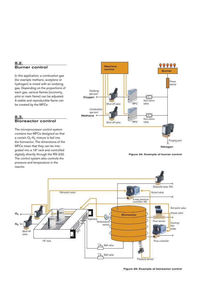
8.2. Burner control

In this application, a combustion gas(for example methane, acetylene orhydrogen) is mixed with an oxidizinggas. Depending on the proportions ofeach gas, various flames (economy,pilot or main flame) can be adjusted.A stable and reproducible flame canbe created by the MFCs.

8.3. Bioreactor control

The microprocessor control systemcontains two MFCs designed so thata certain O2-N2 mixture is fed into the bioreactor. The dimensions of theMFCs mean that they can be inte-grated into a 19” rack and controlled digitally directly through the RS-232.The control system also controls thepressure and temperature in the reactor.

Machine control

Burner

Oxygen

Oxidizing gas port

Shut-off valve MFCNon-return valve

Non-return valveMFCShut-off valve

Methane

Combustiongas port

Flame barrier

Nitrogen

Purging port

O2

N2

Ball valve

Temperaturesensor

Bioreactor

Pressure sensor

Ball valve

19” rack

Shut-off valve

Flow sensor

Flow controller

MFC

MFC

Set-point value Actual value

Actual value

Cooling/Hot water

Solenoid valve, NO

2-way pressure controller, NC

Set-point value

TFT

Keyboard

Figure 25: Example of burner control

Figure 26: Example of bioreactor control

30

9.1.Features of solenoid-operated proportionalvalves

Positioning valves can be combinedwith pneumatic, motorized, piezo-electric or solenoid actuators.The main differences between the various actuation principles are price,type of media separation and dynamicand force properties. Solenoid-oper-ated positioning valves are known inpractice as proportional valves andcover the nominal diameter range below 25 mm. The magnetic force required for larger nominal diameterswould require a coil size that is neitherpractical nor economical.

Open and closed control loops canbe developed using proportional valves. Open control loops control the valve without feedback signal,while closed control loops control the difference between the set-pointand actual values (see Section 9.5,Use of proportional valves in open orclosed control loops). Switching solenoid valves, which are normallyclosed, form the basis for Bürkert pro-portional valves. Making constructivemodifications to switching solenoidvalves can achieve a balance of thespring and magnetic force for any coilcurrent. The level of the coil currentand magnetic force determines thestroke of the plunger or the valve opening, whereby the valve opening and the current are ideally linked by a linear dependence.

Direct-acting proportional valves (up to a nominal diameter of 12 mm) receive their feed below their seat,while servo-assisted models (with anominal diameter over 12 mm) receivetheir feed above their seat. Since themedium pressure (on direct-actingvalves) and magnetic force actagainst the return spring that pressesthe plunger against the seat, it is a good idea to set the minimum andmaximum flow rate of the working range (coil current) in operating con-ditions. Bürkert proportional valvesare normally closed (NC).

9. Propor t ional va lves

30/31

Figure 27: Extract from Bürkert range of control valves

kVs-value (flow of water with a 1 bar pressure drop through the valve and a temperature of 20 °C)

>0 0.5 1.5 2.8 4.5 5.0 140 235

Servo-assisted valves with push-over(Type 6xxx) coil and cable plug controller

Electropneumaticallyoperated control valvesfor primary and secon-dary control loops

Direct-acting valveswith push-over (Type6xxx) or block-assem-bled (Type 28xx) coils

With shut-off valves, the magnetic force, generated by the minimum per-missible switching current, is greaterthan the spring force of the returnspring in every stroke position. Theminimum switch-on current opens thevalve (the curves in Figure 29 apply to normally closed valves). The greaterthe stroke, the smaller the air gap be-tween the armature and the oppositearmature pole, and the lower the re-quired coil current. This is becausethe smaller the air gap, the greater the force of attraction created by themagnets. Proportional solenoids have a considerably different stroke forcecharacteristic map. There is a plateauof at least the length of the workingstroke for all current values. That means that there is a well-defined point of intersection for the magneticforce with the spring force that actsdependent on the stroke. I.e. the current value can be used to de-termine the stroke and therefore theopening of the valve.

Stroke force characteristic curves with a plateau can be obtained bypreventing the large drop in magneticforce with a growing working air gapthat occurs with a flat geometry of the armature and opposite armaturepole, for example by using a conicaltransition area in the outer section ofthe opposite armature pole and a corresponding angle at the top of thearmature (see Figure 28).

Cross section of a direct-acting valve witha block-assembled coil

The coil on the direct-acting propor-tional valve in Figure 30 is secured tothe valve body by four screws (block-assembled). The armature, also knownas the plunger, contains a plungerseal that ensures that the valve is clo-sed tightly by spring force when nocurrent is applied to it. The plunger-type armature is guided by a pin and a glide ring. The PTFE glide ring has a negative effect as a result of thefriction it generates. Minimizing thisfriction is particularly important

inrespect to the hysteresis and re-sponse sensitivity (see Section 9.3,Characteristic parameters of propor-tional valves). This can be achievedthrough perfect guidance of the plunger with low friction glide ringsand electronically by using a suitableactuation system (see Section 9.2,Actuating proportional valves). Thepressure range can be establishedusing the adjusting screw in the op-posite armature pole.

Force F

Magnetic force characteristic with minimum switching current

Magnetic force characteristic curves for shut-off valves

Spring characteristic curve

Stroke h

Force FForce F

Characteristic curves for proportional valvesCharacteristic curves for proportional valves

Spring characteristic curveSpring characteristic curve

CurrentCurrent

Operating rangeOperating range

Stroke hStroke h

Figure 29: Comparison of the characteristic curves of shut-off and propor-tional valves

Oppositearmature pole

Armature

Pilot valve

Profiled armature

Armature

Proportional valve

Oppositearmature pole

Figure 30: Cross section drawing of Type 2834 proportional valve

Figure 28: Comparison of the geometries in the working air gapof shut-off and proportional valves

8 Coil, epoxy-encapsulated

7 Plunger, stainless steel

6 Stopper with integrated adjusting screw, stainless steel

5 Return spring, stainless steel

4 Glide ring, PTFE compound

3 O-ring, Viton (standard)

2 Plunger, Viton (standard)

1 Valve body, brass or stainless steel

3232/33

Cross section of a direct-acting valve withpush-over coil

In addition to direct-acting valves withblock-assembled coils, there are coilsthat are pushed over an armature guidetube and secured with a locknut (Fig-ure 31). Push-over coils can be turn-ed and replaced easily. In contrast to block-assembled valves, the arma-ture is guided by two glide rings.

In newly developed direct-acting pro-portional valves, such as Type 2822,shaped springs, rather than gliderings and spiral springs, are used forguidance and resetting. This form ofguidance results in virtually no friction.The bottom shaped spring guides the plunger while the top one takescare of the resetting action.

Cross section of aservo-assisted valve

In the case of seat valves, for largeflow rates, in other words large nomi-nal diameters, the force requirementson the solenoid actuator increase. The use of direct-acting proportionalvalves for large flow rates would therefore require very large solenoid actuators. For servo-assisted systems(Figure 32), the main seat of the finalcontrol element is not opened andclosed by the solenoid actuator, butrather by a pilot piston.The pilot piston supports the solenoidactuator, thus necessitating less effortand expense.

Figure 33 shows the operating princi-ple of such a valve. When it is closed,the medium at the input side has apressure of p1, the core or plunger (3)has dropped out and therefore presseson the pilot seat (4). As a result of this and the force of the piston spring,which acts on the piston (2), the mainseat (5) is closed. A restrictor port (6)allows the medium to enter the controlchamber (1) and press on the dia-phragm or gasket from above with apressure px. If the coil is operated at a higher current and the plunger istherefore attracted, the medium canescape from the control chamber.

Figure 31: Cross section drawing of a proportional valve with push-over coil

Figure 32: Cross section drawing of a servo-assisted proportional valve

12

5

34

6

px

p1

p2 Flow direction

Figure 33: Diagram of a servo-assisted proportional valve

Flange 11

10 Locknut

9 Coil, polyamide

8 Stopper with integrated adjusting screw, stainless steel


6 Glide ring, PTFE compound

5 Plunger, stainless steel

4 Armature guide tube, stainless steel

3 O-ring, Viton (standard)

2 Plunger seal, Viton (standard)


11 Stopper with adjusting screw, stainless steel


9 Armature guide tube, stainless steel

8 Glide rings, PTFE compound

7 Pilot seat seal, Viton (standard)


5 Pilot seat, PPS

4 Gasket, PTFE

3 O-rings, Viton (standard)

2 Seal, Viton (standard)


Flow direction

Coil, polyamide 16

Plunger, stainless steel 15

Hood, polyamide 14

Piston, PPS 13

Cover, stainless steel 12

c

Flow direction

As soon as the force formed from theproduct of px and the piston surfacearea Ak is lower than the force formedfrom the product of p1 and the circularring surface area (Ak – As), the medium at the input has a supportingrole in opening the main seat. If therestrictor port, pilot seat and area ra-tios on the main stage are rated ac-cordingly, the compression forces onthe piston reach equilibrium when theseat is opened by a certain position.With proportional pilot control, ideally,the piston follows the continuous axialmovement of the plunger precisely atthe distance that creates this equilib-rium. Theoretically, the force require-ment for the pilot solenoids can bedrastically reduced by the parallel re-duction of the pilot seat and the re-strictor port, but its sensitivity to dirt,the negative effects on the dynamics,and friction forces limit this process. A minimum input pressure is requiredfor servo-assisted systems to over-come the frictional forces that counter-act the opening motion of the piston.In addition, it must also overcome theforce of the piston spring, which pri-marily ensures the availability of ade-quate sealing force even if the pressureis low.

9.2.Actuating proportionalvalves

In principle, it is possible to actuatethe proportional solenoid with variableDC voltage, but as a result of the friction on the guiding points of theplunger, this results in poor responsesensitivity and characteristic curveswith high hysteresis and a step struc-ture (stick-slip effect). To prevent this,the standard input signal is convertedinto a continuously varying solenoid excitation. This kind of actuation re-sults in the plunger being made to oscillate constantly around its equili-brium position at low amplitude. Thismeans that it remains in its slidingfriction state. The conventional kind ofactuation is a pulse width modulatedvoltage signal (PWM actuation, seeFigure 34). With PWM actuation, theeffective solenoid current with a con-stant voltage supply is set by the dutycycle of the rectangular signal. ThePWM frequency is tailored to the in-trinsic frequency and attenuation ofthe spring-plunger system as well asthe inductance of the magnet circuit.If the control signal rises (Figure 34,top), the duty cycle t1/T (t1: on time,

T: cycle duration, f = 1/T: frequency)also rises. The effective coil current rises at the same time since the pulsewidth of the rectangular signal increa-ses (Figure 34, bottom).The reference signal is a periodic signal.

Functions of the control electronics

Essentially, the control electronics converts the analog set-point signal at the input into a corresponding pulse width modulated output signal,which is used to control the valve.In addition, the control electronics contains a current control facility tocompensate for coil heating, a facilityto adjust the minimum and maximumcoil current to the pressure conditionsin the specific application, a zeroswitch-off function to close the valveand a ramp function.

■ Current control facility to compensate for coil heatingSince the resistance changes over time as a result of the coil heating, a current control facility is integrat-ed into the control electronics. A current control facility is particularlyimportant in open control loops. The current control facility is irrelevant in closed process control loops.

Reference signal

UU, I

U

t1 t

t

T

Tt1

I

Control signal

24V

Figure 34: Pulse width modulationprinciple sketch

3434/35

9.3.Characteristic para-meters of proportionalvalves

■ kVs-value/QNn-valueValves are comparable in fluidic terms by their kV value (unit: m3/h), which is measured by the flow of water at 20 °C and 1 bar relative pressure at the valve input against 0 bar at the valve output. A secondflow characteristic, the QNn value, is often stated for gases. The QNn

value specifies the standard flow rate in lN/min of air (20 °C) at 6 bar(overpressure) at the valve input and 1 bar pressure loss through the valve. Reference conditions for the gas are 1.013 bar absolute and a temperature of 0 °C (273 K).

■ HysteresisThe maximum difference of the fluidoutput signal as it passes throughthe full electrical input signal rangein the upward and downward di-rections; stated as a percentage of the maximum fluid output signal(the flow rate is assumed for theexample in the sketch). Hysteresis is caused by frictionand magnetization.

■ Adjustment of the minimum and maximum coil current to the pressure conditions in thespecific applicationUnder operating conditions, poten-tiometers can adjust the currentvalues at which the valve starts toopen or reaches its fully open set-ting.

■ Zero switch-off function to close the valve The zero switch-off function en-sures that the valve is closed if the input signal is less than 2 % of the maximum value. The coil current is then set to zero. The zero switch-off function must generally be deactivated to set the minimum coil current.

■ Ramp function Set-point adjustments can be sent to the proportional valve witha delay of 0 – 10 seconds. Sudden changes in the set-pointvalue, which may cause oscillationsin some systems, can thus be suppressed.

■ SensitivitySmallest set-point differential thatresults in a measurable change inthe fluid output signal; stated as apercentage of the maximum fluidoutput signal.

■ LinearityMeasure of the maximum deviationfrom the linear (ideal) characteristiccurve; stated as a percentage ofthe maximum fluid output signal.

Hysteresis

Flow rate

Input signal

Figure 35

Sensitivity

Stroke difference

Set-point differential

Figure 36

Flow rate

Ideal curve, in this case, the mean value curve

Linearity deviation

Inputsignal

Figure 37

■ Repeatability (reproducibility)Range within which the fluid outputvariable deviates if the same elec-trical input signal, coming from the same direction, is set repeatedly; stated as a percentage of the maxi-mum fluid output signal.

■ SpanRatio of the kVs value to the mini-mum kV value at which the charac-teristic curve remains within a tolerance band about the idealcharacteristic curve in terms of its height and gradient.

9.4.Rating of proportionalvalves

To ensure smooth, problem-free con-trol functioning, proportional valvesmust be rated and selected for a spe-cific task. The most important charac-teristic parameters for selecting a proportional valve are the kV value andthe pressure range of the application.In addition to the kV value, the maxi-mum supply or input pressure is themain value required when selecting a valve (type and nominal diameter).The smaller the nominal diameter ofthe valve or the stronger the coil, thegreater the possible maximum pressureit can handle.

The kV value can be calculated usingthe following formulae.Using the calculated kV value and thepressure range of the application, it ispossible to find the valve type usingthe type selection diagram (see Sec-tion 10, Proportional valve range). The kV value of the application mustbe less than the kVs value of the valveachieved when it is fully open.

Flow rate

Repeatability

Inputsignal

Figure 38

kVkVs

Stroke hh100

1

10.02

Figure 39

00.0

0.1

0.2

0.3

0.4

0.5

0.6

0.7

0.8

0.9

1.0

40

51210

10 [V]20 [mA]20 [mA]

kVkVs

Figure 40: Typical flow-rate charac-teristic curve of a proportional valve

Span = kVs/kVmin

3636/37

kV = Characteristic flow rate in m3/h

Q = Flow rate of application in m3/h (Liquids)

QN = Normal flow rate in mN3/h QNn = QN ( p1=7 bar(a), P2 = 6 bar(a), T1=293 K)

p1 = Input pressure in bar(a)1

p2 = Output pressure in bar(a)∆p = p1-p2 in bar� = Density in kg/m3

�N = Normal density in kg/m3

T1 = Medium temperature in (273+t) K

1 bar(a) = absolute pressure, barg

corresponds to the pressure relative to

the atmospheric pressure (1.013 bar)

Conversion from standard or operating into normal conditions:

QS= Flow rate under standard(1.013 bar and 20 °C) or under other operating conditions

pS = Absolute pressure under stand-ard (=1.013 bar) or under other operating conditions

TS = Temperature under standard(=293 K) or under other operat-ing conditions (=(273+t)K)

QN= Normal flow ratepN = Normal pressure

(=1.1013 bar)TN = Normal temperature (= 273 K)

Conversion from kV into QNn

and kV into cV:kV = 1078 · QNn

kV = 0.86 · cV

cV = characteristic flow rate in USgal/min = 0.227 m3/h. Flow rate of water at a tem-perature of 60 °F and at a pressure drop of 1 psi throughthe armature (1 psi = 0.069 bar)

The aim is to avoid a situation wherethe “final few percentage points offlow rate are squeezed out of a sy-stem” by increasing the size of thevalve (kVs) too far. If kVs exceeds theflow-rate coefficient of the system kVa

to a great extent, the valve authority

becomes too low, leading to a situa-tion where only a small proportion ofthe operating range of the valve isused. This can result in impairment ofthe resolution and the general controlquality.In this, (∆p)V0 is the pressure dropthrough the fully opened valve and(∆p)0 is the pressure drop through the entire system.

The valve authority � should not be below 0.3 ... 0.5 in order to ensure anacceptable operating characteristiccurve for the system.

p2 >

p2 <

= Q · �

∆p · 1000�= Q ·

�

∆p · 1000�

Pressure gradient

Sub-critical

Super-critical

Liquids, kv in m3/h Gases, kv in m3/h

= · �N · T1

∆p · p2

QN

514 �= · �N · T1

QN

257 · p1�p1

2

p1

2

TN · pS

Ts · pNQN = QS ·

(∆p)V0

(∆p)0

kVs2

kVa2 + kVs

2� = =

Calculation formulae for determining the kV value

9.5.Use of proportionalvalves in open andclosed control loops

Comparisons of open and closedcontrol loops and continuous andon/off controllersFigure 41 shows a closed controlloop. Without returning the actual val-ue or controlled variable x by using ameasured value pick-up with an inte-gral transducer, an open control loopis produced. The influence of disturb-ance variables (z1, z2), for example coil heating in proportional valves, leads to control differences in opencontrol loops that cannot be compen-sated. The controller finds the controlsignal y depending on the control deviation xw (difference between set-point and actual value). The propor-tional valve is controlled by the manip-ulated variable with the aim of re-ducing or eliminating the deviation in the controlled system. Example: if the water supply to a tankis controlled (open control loop), thetank will overflow or be completelyemptied. Regulating the supply de-

pending on a signal relating to the filling level (level measurement) guarantees that the filling level will be regulated by the set-point value.

When a closed control loop is de-signed, the appropriate controller is selected for a specific controlled system. In addition to knowledge ofthe dynamic and static properties ofthe controlled system, this also re-quires knowledge about the proper-ties of the various controller versionsor controller types.Controllers can be divided into twomain groups, continuous and on/offcontrollers. Continuous controllersoutput a continuous control signal,while on/off versions output a cycledsignal. The positioning valve must therefore be capable of stopping inevery stroke position (positioning range) if a continuous controller isused, while a on/off valve will suffice if an on/off controller is used. De-pending on the cycle frequency, arange of set-point values can be han-dled. The drawback of on/off control-lers is the fluctuation of the actual

value around the set-point value.Examples of on/off controllers are two and three-point controllers.

Continuous (PI) controllersContinuous controllers are used for demanding closed-loop control tasks.There is a whole series of continuouscontrollers, with the main ones in usebeing P, PI, PD and PID controllers.These controller types differ from eachother in terms of their dynamics, in otherwords the speed with which they movethe actual value towards the set-pointvalue depending on the level of controldeviation. These controllers are charac-terized by their step response, or to bemore precise, by the speed with whichthey react after a sudden change in theinput variable, the control deviation xw.

Controller Continuouscontrol valve

Measured value pick-up plus transducer

Comparison point

W Xw Y X

Z 1 Z 2

Tank

Figure 41: General block diagram of the closed control loop

w: Set-point value or reference variable(required filling level)

x: Actual value or controlled variable(measured filling level)

xw: Control deviation (actual value – set-point value), also known as xd

y: Controller out put signal(control variable)

z1: Disturbance variable 1 (outflow from the tank)

z2: Disturbance variable 2 (evaporation of liquid from the tank)

38

Cable plug controllers, as shown inFigure 42, contain a PI controller andcan be mounted directly on propor-tional valves.

The PI algorithm consists of a pro-portional component and an integralcomponent. In a stationary state, thecontrol variable of the proportionalcomponent is directly proportional toits input variable (xw). The control variable of the P-component can becalculated as follows:

y = kp · xw = kp · (w – x)

Depending on kp the control variablemay be less than (kp< 1) or greaterthan (kp > 1) the control deviation. kp is known as the proportional gainfactor or proportional co-efficient.

Characteristics of a pure P controller:■ Operates without delay and very

quickly■ Control loops with a pure P con-

troller have a permanent controldeviation.

The integral component calculates itsshare of the control variable via thetime integral of the control deviation. Ifthere is a control deviation, the integralcomponent increases the control varia-ble. This avoids the permanent controldeviation that occurs on P controllersand PD controllers.

The control variable of a PI controlleris calculated as follows:

As can be seen from the above cal-culation formula for the control varia-ble, the influence of the I-componentis determined by parameter Tn. The lower Tn becomes, the greater the I-component becomes when calcu-lating the control variable. Integral-action time Tn is the time that the con-troller requires to generate a controlvariable of the same magnitude asthat which occurs immediately as theresult of the P-component by meansof the I-component (see Figure 43).

Characteristics of the PI controller:■ Responds quickly (P-component)

and eliminates control deviations(I-component)

■ Better adjustment to controlled system possible, since two para-meters can be adjusted.

Practical experience has shown thatthe following estimate on the suitabilityof conventional controller types canbe made for controlling importanttechnical controlled variables.

38/39

XwInput signal

Input step

Time

Y

Step response

Time

Y = Kp*Xw

Y = 2*Kp*Xw

Tn

Figure 43: Step response of the PI controller

y = Kp*( * (xw(t)dt) + xw(t)) 1Tn

�

Figure 42: Bürkert cable plug con-troller combined with a proportionalvalve

Additional, more detailed control information is contained in our “Competences” brochure.

Table 5: Suitability of various continuous controllers for controlling important technical controlled variables

Controller type

P PD PI PID

Controlled variable Permanent control deviation No permanent control deviation

Temperature Conditionally suitable Conditionally suitable Suitable Suitable for stringent demands

Flow Unsuitable Unsuitable Suitable Over-dimensioned

Pressure Suitable Suitable Suitable Over-dimensioned

Filling level Suitable Suitable Suitable Over-dimensioned

40

10.1.Brief instructions:How to find the rightproportional valve?

1. What medium do you want tocontrol or supply?The parts of the valve that come into contact with the medium must be suitable for it.

2. What is the maximum input pressure?The maximum input pressure p1max

must be checked to ensure that thevalve can completely close against the medium pressure.

3. What are the process data? To achieve the optimal design of thenominal valve diameter, in addition to the required maximum flow rateQnom, the pressure values immediatelyupstream and downstream of the valve(p1, p2) at this flow rate Qnom must beknown. These often differ from the in-put and output pressure of the systemas a whole because both upstream

and downstream of the valve, theremay be additional flow resistors (pipes, shut-off valves, nozzles, etc.). If the input pressure (p1) and outputpressure (p2) are not known or cannotbe obtained by measurement, an esti-mate must be made, taking into ac-count the approximate pressure dropsthrough the flow resistors upstreamand downstream of the valve at Qnom.For rating purposes, it is also neces-sary to provide details of the mediumtemperature T1 and the standard den-sity N of the medium (can be obtain-ed for mixtures using the percentagevalues). The possible measuring spanmust be checked to determine wheth-er the minimum flow rate Qmin can be adjusted.

In the type selection diagram, you can find valves that comply with thefollowing rules:■ kVs of valve > kV of the application

and ■ pressure p1max , that the valve can

switch > pressure p1max , that canapply upstream of the valve.

10. Proport ional valve range

40/41

Table 6: Overview of Bürkert Proportional Valves

Type 28xx 0.8..1.60, 0.018..0.05 12..6 1/8“, flange X X 4W 2821Block-assembled 0.3..1.0 0.002..0.03 10..2 1/8“, flange X X 1W 2822coil 0.8..4.0 0.018..0.33 16..2 1/8“ / 1/4“, flange X X 8W 2832

2..6 0.12..0.65 25..4 3/8“ X X 14W 28343..12 0.25..2.5 25..2 1/2“ / 3/4“ X X 24W 2836

Type 6xxx 0.8..1.6 0.018..0.05 12..6 1/8“ X X 4W 6021Push-over coil 0.8..4.0 0.018..0.33 16..2 1/8“ / 1/4“ X X 8W 6022

10W4..6 0.4..0.7 4..2 3/8“ X X 14W 60238..12 1.4..2.8 0.7..0.2 1/2“ / 3/4“ X X 18W 602410..20 1.4..5.0 10 3/8“–1“ X 8W 6223

10W14W

Nom

inal

di

amet

ers

DN

[mm

]

k Vs ra

nge

[m3/h

]

Max

. ope

ratin

gpr

essu

re

[bar

]

Por

t co

nnec

tions

Gas

es

Flui

ds

Max

. pow

erco

nsum

ptio

n

Type

�

10.2.Type selection diagrams

Table 7: kVs ≤ 0.05 m3/h


kVs DN Max. operating pressure [bar] Type[m3/h] [mm] 0 0.2 0.4 0.5 0.7 1 1.5 2 3 3.5 4 5 6 8 10 12 16 250.002 0.3 2822

0.004 0.4 2822

0.01 0.6 2822

0.018 0.8 2822

0.025 1.0 2822

0.018 0.8 28216021

0.025 1.0 28216021

0.04 1.2 28216021

0.05 1.6 28216021


60220.04 1.2 2832

60220.06 1.5 2832

60220.01 2.0 2832

60220.15 2.5 2832

60220.23 3.0 2832

60220,33 4,0 2832

60220.12 2.0 2834

0.25 3.0 2834

0.4 4.0 2834

0.7 6.0 2834

0.4 4.0 6023

0.7 6.0 6023

4242/43


0.4 4.0 2836

0.9 6.0 2836

1.4 8.0 2836

2 10.0 2836

2.5 12.0 2836

1.4 8.0 6024

2 10.0 6024

2.8 12.0 6024

1.4 10.0 6223

2.5 13.0 6223

5 20.0 6223


Set

-poi

nt v

alue

Set

-poi

ntva

lue

Act

ual v

alue

Act

ual v

alue

Act

ual v

alue

Act

ual v

alue

1094

1094

1094

Set

-poi

ntva

lue

Set

-poi

nt v

alue

Actual value

Set-pointvalue

Valve 2832, 2834, 2836, 6022, 6023, 6024, 6223

Cable plug –

Controller 1094

–

2821, 2822, 6021

2506, 2507 (28xx)

1094

–

2832, 2834, 2836, 6022, 6023, 6024, 6223

2508

1094

–

2832, 2834, 6022, 6023, 6024, 6223

–

–

8623-2, 8624-2, 8625-2

Figure 44: Possible combinations of Bürkert actuators with Bürkert Proportional Valves

Open control loop (control mode) Closed control loop

10.3.Overview of possible actuators

Set

-poi

nt

valu

e

Set

-poi

nt

valu

e

4444/45

11. Type descr ip t ions of propor t ional va lves and actuators

Data:■ For neutral gases or liquids

and vacuum■ kVs values 0.018 to 0.05 m3/h■ Max. operating pressure depending

on nominal diameter, 12 bar (175psi) (DN 0.8)

■ Stainless steel or brass valve body■ Viton seals, EPDM or PTFE on

request■ Hysteresis < 5 %■ Repeatability < 0.5 % F.S. ■ Span 1:25■ Medium temperature –10 to +90 °C

■ Type of protection IP 65■ Operating voltage 24 V DC■ Power consumption 4 W■ Control signal pulse width

modulated (PWM)

Characteristics:■ Process and product optimization

as a result of continuous control■ Tight-closing function in the event

of power failure■ High repeatability■ PWM control reduces stick-

slip risk■ Very short response time

(20 – 30 ms)

11.1. Type 2821

Direct-acting 2/2-way Proportional Valve; 1/8” or flange (DN 0.8 – 1.6 mm)

11.2. Type 2822

Direct-acting 2/2-way Proportional Valve; 1/8” or flange (DN 0.3 – 1.0 mm)

Data:■ For neutral gases or liquids and

vacuum■ kVs values 0.002 to 0.027 m3/h■ Max. operating pressure depending

on nominal diameter■ Stainless steel or brass valve body■ Viton seals, EPDM or PTFE on

request■ Hysteresis < 10 %■ Repeatability < 0.25 % F.S. ■ Span 1:500■ Medium temperature

– 10 to + 90 °C■ Type of protection IP 65■ Operating voltage 12 V or 24 V DC

■ Power consumption depending onnominal diameter, min.1W, max. 4 W

■ Control signal pulse width modulated (PWM)


as a result of continuous control■ Excellent span■ Good sensitivity

(< 0.1 % F.S.)■ High repeatability■ Low-friction and low-noise valve,

PWM control not necessary■ Low-power and low-flow valve■ Very short response time (< 20 ms)

Figure 45: Proportional Valve, Type 2821

Figure 46:Proportional Valve, Type 2822



on nominal diameter, 16 bar (DN 0.8, 230 psi)


request■ Hysteresis < 5 %■ Repeatability < 0.5 % F.S. ■ Span 1: 25■ Medium temperature

– 10 to + 90 °C■ Type of protection IP 65

■ Operating voltage 24 V DC■ Power consumption 8 W■ Control signal pulse width

modulated (PWM)■ Option EEx ed II C T4/ATEX/

Zone 2, 22




slip risk■ Very short response time (50 ms)

11.3. Type 2832

Direct-acting 2/2-way Proportional Valve; 1/8”, 1/4” or flange (DN 0.8 – 4.0 mm)



on nominal diameter, 25 bar■ Stainless steel or brass valve body■ Viton seals, EPDM or PTFE on


– 10 to + 90 °C■ Type of protection IP 65■ Operating voltage 24 V DC■ Power consumption 14 W

■ Control signal pulse width modulated (PWM)

■ Option EEx m II T4/ATEX/Zone 2, 22

■ Option steam design up to max. +140 °C.



of power failure■ High repeatability■ PWM control reduces

stick-slip risk■ Very short response time

11.4. Type 2834

Direct-acting 2/2-way Proportional Valve; 3/8” (DN 2 – 6 mm)



4646/47



on nominal diameter, 25 bar (DN 3,360 psi)


request■ Hysteresis < 5 %■ Repeatability < 1 % F.S.■ Span 1:25■ Medium temperature

– 10 to +90 °C■ Type of protection IP 65


modulated (PWM)■ Option steam design up to

max. +140 °C.



of power failure■ Good repeatability■ PWM control reduces stick-


11.5. Type 2836

Direct-acting 2/2-way Proportional Valve; 1/2” or 3/4” (DN 3 – 12 mm)

Data:■ For operation in closed control

loops■ For neutral gases or liquids and




request■ Hysteresis < 5 %■ Repeatability < 0.5 % F.S.■ Span 1:20■ Medium temperature

– 10 to + 90 °C


modulated (PWM)



of a power failure■ High repeatability■ PWM control reduces stick-


(20 – 30 ms)

11.6. Type 6021

Direct-acting 2/2-way Proportional Valve; 1/8” (DN 0.8 – 1.6 mm)










modulated (PWM)■ Option EEx m/em II T4,

TU –30 to +60 °C/ATEX/Zone 1, 21, 2, 22





11.7. Type 6022

Direct-acting 2/2-way Proportional Valve; 1/8” or 1/4”(DN 0.8 – 4.0 mm)


loops■ For neutral gases or liquids and


on nominal diameter, 4 bar (DN 4, 60 psi)


request■ Hysteresis < 5 %■ Repeatability < 0.5 % F.S.■ Span 1:10■ Medium temperature

– 10 to + 90 °C


modulated (PWM)





11.8. Type 6023

Direct-acting 2/2-way Proportional Valve; 3/8” (DN 4 or 6 mm)



4848/49

Data:■ For applications with low operating

pressures (< 700 mbar, e.g. naturalgas)

■ For neutral gases or liquids and vacuum

■ kVs values 1.4 to 2.8 m3/h■ Max. operating pressure depending

on nominal diameter, 700 mbar (DN 8, 10psi)


request■ Hysteresis < 7 %■ Repeatability < 0.5 % F.S■ Span 1:25

■ Medium temperature – 10 to + 90 °C


modulated (PWM)





11.9. Type 6024

Direct-acting 2/2-way low-�p Proportional Valve; 1/2” or 3/4”(DN 8 – 12 mm)


loops■ For neutral liquids■ kVs values 1.4 to 5.0 m3/h■ Max. operating pressure 10 bar

(145 psi)■ Minimum �p = 0.5 bar ■ Brass valve body■ Viton seals, EPDM or PTFE on

request■ Hysteresis < 5 %■ Repeatability < 1 % F.S.■ Span 1:10■ Medium temperature


■ Operating voltage 24 V DC■ Power consumption depending

on nominal diameter, 15 W■ Control signal pulse width

modulated (PWM)




slip risk■ Good response time (< 200 ms)

11.10. Typ 6223

Servo-assisted 2/2-way high-flow Proportional Valve; 3/8” – 1” (DN 10 – 20 mm)



Data:■ Control electronics either as

plug-on module or as a DIN-railmounting version

■ 1 standard signal input for set-point value

■ 1 PWM signal output for valve control (max. 800 Hz, version forType 2822 max. 6 kHz)

■ Max. output current to valve 1.1 A■ Operating voltage 24 V DC■ Max. power consumption 0.5 W■ Max. ambient temperature 55 °C

■ Dimensions:32 x 90 x 42 mm (plug-on module)46 x 76 x 31 mm (DIN-rail mountingversion)

■ Type of protection IP 65 (plug-onmodule)

Additional functions:■ Temperature compensation for

heating of the coil by integrated current control

■ Ramp function for damping suddencontrol signal changes

■ Adjustment of minimum and maximum flow to the real pressure conditions

■ Zero switch-off function

11.11. Type 1094

Control electronics for proportional valves

Figure 55: Control electronics, Type 1094 (top hat rail version)

Figure 56: Control electronics, Type 1094, mounted on a propor-tional valve

5050/51

Data:■ For liquids■ 2 frequency inputs for actual value

(2 – 1000 Hz), e.g. for ratio control■ 1 standard signal input for set-point

value■ 1 PWM signal output for valve

control (max. 400 Hz)■ Accuracy 1 % F.S.■ Max. output current to valve 1 A■ Max. output current to sensor 0.5 A■ Operating voltage 24 V DC■ Max. power consumption 1.5 W■ Set-point value internal or external■ Input signals scalable■ Ambient temperature

– 10 to + 60 °C■ Dimensions 54 x 54 x 61 mm,

polyamide■ Type of protection IP 65

■ Certified electromagnetic compatibility

■ Optional field bus communication

Characteristics:■ Fast and easy installation■ High reliability due to decentralized

intelligence■ Clear LCD display■ Programming of various ■ functions■ Tight-closing function

Programming:■ Selection of internal or external

set-point value ■ Setting of control parameters■ Selection of inverted or non-

inverted control■ Zero switch-off function■ Setting the unit and scaling

11.12. Type 8623-2

Compact flow controller for direct mounting2 frequency inputs (actual value); 1 standard signal input (set-point value); 1 PWM signal output

Data:■ For flowing gases or liquids■ Standard signal input for actual

value■ Standard signal input for set-

point value■ 1 PWM signal output for valve

control (max. 400 Hz)■ Max. output current to valve 1 A■ Max. output current to sensor 0.5 A■ Operating voltage 24 V DC■ Max. power consumption 1.5 W

■ Set-point value internal or external■ Input signals scalable 0 – 30 bar

(435 psi) ■ Ambient temperature

– 10 to + 60 °C■ Dimensions 54x54x61 mm,

polyamide■ Type of protection IP 65■ Certified electromagnetic

compatibility■ Optional field bus communication

11.13.Type 8624-2

Compact flow pressure controller for direct mounting1 standard signal input (actual value) and 1 standard signal input (set-pointvalue); 1 PWM signal output

Figure 57: Cable plug controller, Type 8623-2,mounted on a proportional valve


Data:■ 1 Pt100 signal sensor input■ 1 standard signal input for set-point

value■ 1 PWM signal output for valve

control (max. 400 Hz)■ Max. output current to valve 1 A■ 0.5 mA output for Pt100 sensor■ Operating voltage 24 V DC■ Max. power consumption 1.5 W■ Set-point value internal or external■ Input signals scalable

– 50 to + 150 °C (– 58 to 302 °F)■ Resolution 0.25 °C■ Accuracy 1 °C■ Ambient temperature

– 10 to + 60 °C■ Dimensions 54x54x61 mm,

polyamide■ Type of protection IP 65■ Certified electromagnetic compati-

bility■ Optional field bus communication


intelligence■ Clear LCD display■ Programming of various functions■ Tight-closing function




11.14.Type 8625-2

Compact temperature controller for direct mounting1 Pt100 signal input (actual value); 1 standard signal input (set-point value);1 PWM signal output


intelligence■ Clear LCD display■ Programming of various functions■ Tight-closing function■ Suitable for use as general-purpose

controller for all controlled variables





5252/53

12. Appl icat ion example

Flow control Pressure control

Flow control

Anode side

H2

Pressure sensor, Type 8323

Set-pointType 8624-2

Type 2834

Type 8623-2

Set-point

De-ionized water

Type 6022Flow sensor,Type 8045

2-way pressure control

Condensate draining valve onH2 end, Type 6125

Humidifier

Unobstructed output

Hydrogen

Mass Flow Controller, Type 8626

Set-point

Type 8623-2

Type 8045

Type 6022

Type 8626

Type 8323

Type 8624-2

Type 2834

Type 6125

Type 8625

Type 6223

Type 8417

Type 6125

Type 8323

Type 8624-2

Type 2834

Type 8623-2

Type 6022

Type 8045

Flow control

Temperature control

Flow control

Heat exchanger


Pump

Temperature sensor,

Type 8417

Cathode side

O2

Type 6223

Pressure sensor, Type 8323


Type 2834

Type 8623-2

Set-point

De-ionized water

Type 6022 Flow sensor, Type 8045

2-way pressure control

Condensate draining valve onO2 end, Type 6125

Fuel cell

Humidifier

Unobstructed output

Oxygen

Mass Flow Controller, Type 8626

Set-point

Temperature control Pressure control

5454/55

13. Convers ion of var ious uni ts

TemperatureCelsius Kelvin Fahrenheit

x °C – = (x + 273.15) K = (9

x + 32) °F–5

x K = (x – 273.15) °C –

x °F =5

=5

– · – · (x – 32) °C (– · [x – 32] + 273.15) K –= (9

[x - 273,15] + 32) °F9 9 5

5 5

– · ( = (9

[x - 273.15] + 32) °F5

PressurePa mWC Torr Inch H2O psi

1 bar 100000 10.20 750.1 401.6 14.505

mWC: meter water columnpsi: pound per square inch

Flow ratesccm slpm scfm

1 lN/min 1073.22 1.073 30.391 mN

3/h 63.4 0.063 1.82

Reference conditions■ Standard (Index "N”):

1013.25 mbar/273.15 K■ Normal (Index "s”):

1013.25 mbar/293.15 K

Lengths■ 1 inch [in] = 2.54 cm = 0.0254 m■ 1 foot [ft] = 30.48 cm = 0.3048 m■ 1 yard [yd] = 0.9144 m

Volume■ 1 cubic inch = 16.387 cm3

■ 1 cubic foot = 28.317 dm3

■ 1 cubic yard = 0.76455 m3

■ 1 gallon (GBr) [gal] = 4.54609 dm3 = 4.54609 l

■ 1 gallon (USA) [gal] = 3.78543 dm3

sccm: standard cubic centimeter per minuteslpm: standard liter per minutescfm: standard cubic foot per minute

AAccuracy Page 14Actual value Page 13Adjusting screw Page 30Anemometer Page 11Autotune Page 17

BBinary input Page 19Binary output Page 19Block assembled coil Page 30Bypass CMOS sensor Page 17Bypass sensor Page 16Bypass unit Page 11

CCable plug controller Page 37Calibration curve Page 12Calibration medium Page 13Calibration protocol Page 12Calibration Page 12Communication LED Page 19Communication software Page 29Configurator Page 22Continuous controllers Page 37Control deviation Page 13Control dynamics Page 17Control electronics Page 17Control variable Page 13Conversion factor Page 12Current control facility to compensate for coil heating Page 33Cv value Page 36

DDirect-acting proportionalvalves Page 30Display of operating status Page 19Durty cycle Page 33

EError LED Page 19

FField bus Page 19Flow conditioning Page 11Flow controller Page 50Flow-pressure controller Page 50Full scale value range Page 13

GGas mixture Page 12General-purpose controller Page 50

HHeat capacity, specific Page 11Heat conductivity Page 11Hysteresis Page 34

IInline sensor Page 15Input filter Page 13Integral-action time Page 38

KkVs value Page 34

LLaminar flow element Page 13Limit switch Page 20Limit(y) LED Page 19Linearity Page 34

MMass Flow Communicator Page 20Mass flow Page 9Measurement bridge circuit Page 11Measuring resistors Page 11Microprocessor electronics Page 17

NNominal flow rate Page 13

OOn time Page 33Operating medium Page 13

PPower LED Page 19Profiled armature Page 30Proportional coefficient Page 37Push-over coil Page 30PWM control Page 33PWM frequency Page 33

QQNn value Page 34

RRamp function Page 33Rating data Page 22Reference conditions Page 9Relay output Page 19Repeatability Page 35Reproducibility Page 35Response time Page 13RS-232 Page 19RS-485 Page 19

SSafety value Page 19Sealing function Page 19Self-optimizing routine Page 17Servo-assisted proportional valves Page 30Sensitivity Page 34Set-point profile Page 20Set-point value Page 13Settling time Page 13Span Page 35Specification sheet Page 22Standard volume flow Page 10Step response Page 17Stroke forcecharacteristic curve Page 31Sub-critical pressure gradient Page 35Super-critical pressure gradient Page 35

TTemperature controller Page 51Totalizer Page 20

VValve authority Page 35Volume flow Page 9

ZZero switch-off function Page 33

14. L is t o f keywords

56/59

Burkert Service and Distribution Network

AustraliaBurkert Fluid Control SystemsNo. 2 Welder Road,Seven Hills, NSW 2147Tel. +61 1300 888 868Fax +61 1300 888 076

AustriaBurkert-Contromatic Ges.m.b.H.Diefenbachgasse 1-3 1150 Wien (Vienna)Tel. +43 (0) 1 894 13 33Fax +43 (0) 1 894 13 00

BelgiumBurkert-Contromatic SABijkhoevelaan 32110 WijnegemTel. +32 (0) 3 325 89 00Fax +32 (0) 3 325 61 61

BrazilBurkert-Contromatic Brasil Ltda.Rua Américo Brasiliense no. 2171 cj 100704715-005 São Paulo - SPTel. +55 (0) 11 5182 0011Fax +55 (0) 11 5182 8899

CanadaBurkert Contromatic Inc.760 Pacific Road, Unit 3Oakville (Ontario) L6L 6M5Tel. +1 905 847-55 66Fax +1 905 847-90 06

ChinaBurkert Contromatic (Suzhou) Co., Ltd.9-2 Zhu Yuan Road,Suzhou New DistrictJiangsu, China. 215011Tel. +86 512 6808 19 16Fax +86 512 6824 51 06

Czech RepublicBurkert-Contromatic Ges.m.b.H.Branch-Office AustriaKrenova 35602 00 BrnoTel. +42 05 43 25 25 05Fax +42 05 43 25 25 06

DenmarkBurkert-Contromatic A/SHørkær 242730 HerlevTel. +45 44 50 75 00Fax +45 44 50 75 75

FinlandBurkert OyAtomitie 500370 HelsinkiTel. +358 (0) 9 549 70 600Fax +358 (0) 9 503 12 75

FranceBurkert Contromatic FranceRue du GiessenBP 2167220 Triembach au ValTel. +33 (0) 3 88 58 91 11Fax +33 (0) 3 88 57 20 08

GermanyBürkert GmbH & Co. KGChristian-Bürkert-Straße 13-17D-74653 IngelfingenTel. +49 (0) 7940 10 111Fax +49 (0) 7940 10 448

Hong KongBurkert-Contromatic (China/HK) Ltd.Unit 708, Prosperity Centre77-81, Container Port RoadKwai Chung N.T., Hong KongTel. +85 2 2480 1202Fax +85 2 2418 1945

ItalyBurkert Contromatic Italiana S.p.A.Centro Direzionale „Colombirolo“Via Roma 7420060 Cassina De´Pecchi (Mi)Tel. +39 02 95 90 71Fax +39 02 95 90 72 51

JapanBurkert-Contromatic Ltd.1-8-5 Asagaya MinamiSuginami-kuTokyo 166-0004Tel. +81 (0) 3 5305 3610Fax +81 (0) 3 5305 3611

KoreaBurkert Contromatic Korea Co., Ltd.287-2, Doksan 4 DongKumcheon-kuSeoul 153-811Tel. +82 (0) 3 3462 5592Fax +82 (0) 3 3462 5594

NetherlandsBurkert-Contromatic BVComputerweg 93542 DP UtrechtTel. +31 (0) 346 58 10 10Fax +31 (0) 346 56 37 17

New ZealandBurkert Contromatic Ltd.2A, Unit L, Edinburgh StPenrose, AucklandTel. +64 (0) 9 622 2840Fax +64 (0) 9 622 2847

NorwayBurkert Contromatic A/SHvamstubben 172013 SkjettenTel. +47 63 84 44 10Fax +47 63 84 44 55

PhilippinesBurkert Contromatic Philippines, Inc.8467 West Service RoadSouth Superhighway, SunvalleyParanaque City, Metro ManillaTel. +63 2 776 43 84Fax +63 2 776 43 82

PolandBurkert-Contromatic Ges.m.b.H.Branch-Office AustriaBernardynska street 14 a02-904 WarszawaTel. +48 22 840 60 10Fax +48 22 840 60 11

PortugalBurkert ContromaticTel. +351 21 382 80 00Fax +351 21 387 36 79

SingaporeBurkert Contromatic Singapore Pte. Ltd.51 Ubi Avenue 1, #03-14Paya Ubi Industrial ParkTel. +65 6844 2233Fax +65 6844 3532

South AfricaBurkert Contromatic (Pty) Ltd.233 Albert Amon RoadMillenium Business ParkMeadowaleEdenvaleTel. +27 (0) 11 397 2900Fax +27 (0) 11 397 4428

SpainBurkert Contromatic S.A.Avda. Barcelona, 4008970 Sant Joan Despi (Barcelona)Tel. +34 93 477 79 80Fax +34 93 477 79 81

SwedenBurkert-Contromatic ABSkeppsbron 13 B211 20 MalmöTel. +46 (0) 40 664 51 00Fax +46 (0) 40 664 51 01

SwitzerlandBurkert-Contromatic AG SchweizBösch 716331 HünenbergTel. +41 (0) 41 785 66 66Fax +41 (0) 41 785 66 33

TaiwanBurkert Contromatic Taiwan Ltd.3F, No. 475, Kuang-Fu South RoadTaipei, TaiwanTel. +886 (0) 2 2758 3199Fax +886 (0) 2 2758 2499

TurkeyBurkert Contromatic AkiskanKontrol Sistemleri Ticaret A.S.1203/8 Sok. No 2-EYenisehir, IzmirTel. +90 (0) 232 459 53 95Fax +90 (0) 232 459 76 94

United KingdomBurkert Fluid Control SystemsBrimscombe Port Business ParkBrimscombe, Stroud, Glos., GL5 2QFTel. +44 (0) 1453 73 13 53Fax +44 (0) 1453 73 13 43

USABurkert Contromatic USA2602 McGaw AvenueIrvine, CA 92614U.S.A.Tel. +1 949 223 3100Fax +1 949 223 3198

Systemkatalog 6

Magnetventile I Prozess- und Regelventile I Pneumatik

Sensoren I MicroFluidics I MFC und Proportionalventile


Systemkatalog 1




Systemkatalog 2




Systemkatalog 5




Service brochure

A systematic overview of the

range of products and services

offered by Bürkert. A network of

comprehensive solutions inte-

grating coordinated services.

Competence brochures

Essential information for the person

planning control loops and field

bus systems and who wants to

ensure basic knowledge of the

structure and selection of system

components.

Application brochures

Example applications for deriving

the appropriate system solution,

supplemented by information on

product advantages, user advan-

tages and the range of products

specifically available.

System catalogs

Background knowledge on product

technology, including an up-to-date

overview of the current offers.

Rounded out with information to

help you make your decision on

the best application option.

Technical data sheets

Detailed technical information

for checking specific suitability.

In addition, all the data needed

for direct ordering.

Information paves the path to the appropriate system solution. We provide five

different levels for accessing information, products and services, so that you can

easily find out everything you need to know to make the right choice.

8942

51/

09/0

3/ B

urea

u S

chirl

e

Bürkert Fluid Control Systems, Christian-Bürkert-Straße 13–17, 74653 Ingelfingen, Germany

Tel.+49 (0) 79 40/10-0,Fax+49 (0) 79 40/10-204, [email protected], www.buerkert.com

MFC and proportional valves - cms.esi.info

Documents

Transcript of MFC and proportional valves - cms.esi.info