Metrology-Based Process Modelling

Framework for Digital and Physical

Measurement Environments Integration

Xi Zhang

A thesis submitted for the degree of Doctor of Philosophy

University of Bath

Department of Mechanical Engineering

October 2013

COPYRIGHT

Attention is drawn to the fact that copyright of this thesis rests with the author. A copy

of this thesis has been supplied on condition that anyone who consults it is understood

to recognise that its copyright rests with the author and that they must not copy it or

use material from it except as permitted by law or with the consent of the author.

This thesis may be made available for consultation within the University Library and

may be photocopied or lent to other libraries for the purposes of consultation.

Signature:…………………………………………………

I

Abstract

Process modelling is the activity of constructing and analyzing models, which are

applicable and useful to solve predefined problems. It allows engineering process to

be analyzed, and consequently leads to quality and efficiency improvement. As

metrology becomes increasingly important in modern manufacturing, process

modelling based on measurement techniques and operations becomes necessary and

valuable. Measurement uncertainty, which is obtained from measurement operation, is

regarded as a key factor in metrology-based process modelling. By analyzing

measurement uncertainty, metrology-based process models can tangibly improve

manufacturing quality and efficiency, improve the actualize communication between

design and manufacturing, and, ultimately, achieve product lifecycle integration

between design, manufacturing and verification functions.

Digital measurement models can simulate measurement process, and predict

task-specific measurement uncertainty in the digital environment, before carrying out

capital-consuming physical measurements. However, the integration between digital

and physical measurement environments is not fully approved. Measurement

uncertainty predicted by the digital measurement model may show little practical

significance with that obtained from physical measurements. The quality of digital

measurement result highly relies on input quantities loaded into the digital

measurement model. And it is hardly possible to verify digital measurement results

for all of the measurement scenarios because of the high variability and complexity of

inspected features and measurement tasks.

This research has reviewed the fundamental technologies relating to measurement

process modelling and measurement uncertainty evaluation in a digital environment,

especially for coordinate measurement machines (CMMs). An initial verification

work has been carried out by ‘measuring’ small features on a large-volume

component in a realistic shop floor environment. This verification work has realized

the limitations of the digital measurement model, and the challenge of integrating

digital and physical measurement environments.

II

Based on the initial verification work, a Measurement Planning and Implementation

Framework has been proposed, aiming to analyse and improve the relationship

between digital and physical measurement environments. The Framework is deployed

with the statistics methods to analyse measurement uncertainty obtained from the

digital and the physical measurement environments, and quantitatively predict

influence levels of measurement uncertainty contributors. The verification work of the

Framework has been carried out in a finely-control laboratory environment with

environmental control. The robustness of the Framework has been evaluated,

indicating the potential of deploying statistical methods for measurement uncertainty

analysis, which extends the utilization of measurement uncertainty for

decision-making processes.

The contributions to knowledge of the research include:

(1) Verification of the performance of a digital CMM model under meaningful

measurement scenarios;

(2) Development of a metrology-based process modeling framework to integrate

digital and physical measurement environments through quantitative measurement

uncertainty analysis.

III

Acknowledgement

Thank you to my supervisor, Prof. Paul Maropoulos, for the wide opportunities over

the past few years. Thanks too to all of the ‘The Laboratory for Integrated Metrology

Applications (LIMA)’ at Bath for making my PhD research such a valuable learning

process.

I have greatly appreciated for being supported by Mr. Nick Orchard and Mr. Per

Saunders, from Rolls-Royce Plc, for making the research rich with practical data and

giving me vital experience in shop floor environment. Thanks to Prof. Alistair Forbes

and Dr. Alan Wilson, from the National Physical Laboratory (NPL), UK, for the

intensive laboratory work which has leaded the scientific analysis and argumentation

of the thesis. And thanks to Dr. Jon Balwin, from MetroSage, USA, and Mr. John

Horst, from the National Institute of Standards and Technology (NIST), USA, for

explaining the latest developments of quality system integration. And thanks to Prof.

Tang Xiaoqing and Dr. Du Fuzhou, from Beihang University, China, for helping me

to structure the thesis. Thank you all for the enjoyable and beneficial workshops

throughout my PhD research.

At last, I would like to thank my parents for all their love, patience and support.

IV

Contents

Abstract………………………………………………..………….……………………I

Acknowledgement………………………………………………………….…………II

Contents………………………………………………………………………………IV

List of Figures………………………………………………………………………..IX

List of Tables………………………………………………………………………..XII

Chapter 1 Introduction………………………………………………………………...1

1.1 Background ............................................................................................... 2

1.1.1 Metrology and measurement in high-value manufacturing ............... 2

1.1.2 Measurement process modelling ........................................................ 3

1.1.3 Measurement uncertainty and uncertainty analysis ........................... 6

1.2 Overall aims .............................................................................................. 7

1.3 Organization of the thesis ......................................................................... 7

Chapter 2 Literature Review ...................................................................................... 9

2.1 Fundamentals of coordinate measurement ................................................ 9

2.1.1 Fundamentals of measurement uncertainty ....................................... 9

2.1.2 GD&T standards - ASME Y14.5M ............................................. 14

2.1.3 ISO GPS framework for CMM measurement ................................. 17

2.1.4 Summary .......................................................................................... 25

2.2 CMM Measurement Planning and Modelling ........................................ 26

2.2.1 Inspection feature selection .............................................................. 27

2.2.2 Inspection sequence optimization .................................................... 29

2.2.3 Detailed probing strategy ................................................................. 31

2.2.4 Probing path generation ................................................................... 34

2.2.5 Post-measurement data processing .................................................. 35

2.2.6 Summary .......................................................................................... 37

2.3 Evaluation of task-specific measurement uncertainty using simulation . 41

2.3.1 Requirements of uncertainty evaluating software (UES) as specified

in ISO standard ............................................................................................ 41

2.3.2 The simulation methods for evaluating task-specific measurement

uncertainty .................................................................................................... 42

2.3.3 The verification of UES performance .............................................. 49

2.4 Chapter summary .................................................................................... 53

V

Chapter 3 Research Aims, Objectives and Methodology ........................................ 54

3.1 Aim of the Research ................................................................................ 54

3.2 Objectives of the Research ...................................................................... 54

3.3 Methodology of the Research ................................................................. 55

3.3.1 Research methods in engineering .................................................... 55

3.3.2 Methods for this research project ..................................................... 56

Chapter 4 Initial Study of Establishing Task Specific Uncertainty using a Digital

CMM Model and Physical Measurements ................................................................... 61

4.1 Introduction to the Digital CMM Model ................................................ 61

4.1.1 Working principle ............................................................................ 61

4.1.2 Operations flow ................................................................................ 62

4.1.3 The outputs ....................................................................................... 67

4.2 Pilot case study on verifying Digital CMM Model simulation results by

physical measurements on a large scale component ............................................ 68

4.2.1 Background ...................................................................................... 68

4.2.2 Physical measurements on a large-scale part with relatively

small-size feature ......................................................................................... 69

4.2.3 Simulation measurement results using Simulation-by-Constrain

(SBC) method .............................................................................................. 74

4.2.4 Measurement results comparison ..................................................... 76

4.2.5 Examining the impacts of measurement uncertainty contributors ... 86

4.2.6 In-depth analysis on the hole position measurement results ............ 93

4.2.7 Summary .......................................................................................... 96

4.3 Chapter summary .................................................................................... 97

Chapter 5 A Measurement Planning and Implementation Framework to Compare

Digital and Physical Measurement Uncertainty .......................................................... 98

5.1 Introduction ............................................................................................. 98

5.2 The limitations of task-specific uncertainty simulation model ............... 99

5.3 Examining uncertainty contributor effects by using Design of

Experiments (DOE) approach ............................................................................ 100

5.4 Design of a generic framework to compare digital and physical

measurement environments ............................................................................... 106

5.4.1 The ‘Task-specific Measurement Uncertainty Contributors’ ........ 108

5.4.2 The ‘Measurement Scenario Streamliner’ module ........................ 108

VI

5.4.3 The ‘Measurement Uncertainty Simulation’ module .................... 109

5.4.4 The ‘Physical Verification Process’ ............................................... 109

5.4.5 The ‘Post-Measurement Data Analyzing’ module ........................ 110

5.4.6 Comparison .................................................................................... 110

5.5 Overview of framework methodologies ............................................... 111

5.5.1 Task-specific measurement uncertainty contributors .................... 111

5.5.2 ‘Measurement Scenario Streamliner’ module: Taguchi experimental

design 112

5.5.3 Measurement Uncertainty Simulation module: the

simulation-by-constraints method .............................................................. 114

5.6 Overview of framework implementation .............................................. 116

5.6.1 Measurement uncertainty generation using the simulation software

116

5.6.2 Determining the uncertainty of physical measurements ................ 120

5.6.3 Evaluating the influence levels of uncertainty contributors .......... 121

5.7 Chapter summary .................................................................................. 125

Chapter 6 Experimental Work to Validate the Framework ................................... 126

6.1 Overall experiment plan ........................................................................ 126

6.2 Experiment procedures in the digital environment ............................... 129

6.2.1 Define the part and features to be measured .................................. 129

6.2.2 Select the measurement uncertainty contributors and their factorial

levels ……………………………………………………………………133

6.2.3 Reduce the number of measurement scenarios given to Taguchi

Orthogonal Array ....................................................................................... 141

6.2.4 The measurement process in the digital CMM model ................... 147

6.2.5 Collect simulation results ............................................................... 168

6.3 Digital measurement results and Taguchi experimental analysis ......... 168

6.3.1 Digital measurement results ........................................................... 168

6.3.2 Taguchi experimental analysis of digital measurement results ..... 171

6.3.3 Conclusion of the Taguchi experiment in digital environment ..... 184

6.4 Experiment procedures in the physical environment ............................ 185

6.4.1 Assessing and selecting measurement resources ........................... 186

6.4.2 Defining measurement environment and artefact .......................... 188

6.4.3 Performing physical measurements ............................................... 189

VII

6.5 Physical measurement results and Taguchi experimental analysis ....... 191

6.5.1 Physical measurement results ........................................................ 191

6.5.2 Taguchi experimental analysis of physical measurement results .. 193

6.5.3 Conclusion of Taguchi experiment method in physical environment

……………………………………………………………………204

6.6 Comparison between physical measurement results and digital

measurement results ........................................................................................... 204

6.6.1 Direct comparison .......................................................................... 204

6.6.2 Taguchi experimental result comparison ....................................... 210

6.6.3 Conclusion ..................................................................................... 220

6.7 Chapter Summary ................................................................................. 221

Chapter 7 Conclusions and Further Work ............................................................. 223

7.1 Conclusions ........................................................................................... 223

7.2 Contribution to knowledge ................................................................... 223

7.3 Future work ........................................................................................... 226

Appendix A. Data collection of the simulation results ............................................... 228

Appendix B. Example of Taguchi design of experiments .......................................... 230

Appendix C. Data Collection Sheet to record the digital and physical measurement

results………………………………………………………………………………..234

Reference ………………………………………………...………………………237

VIII

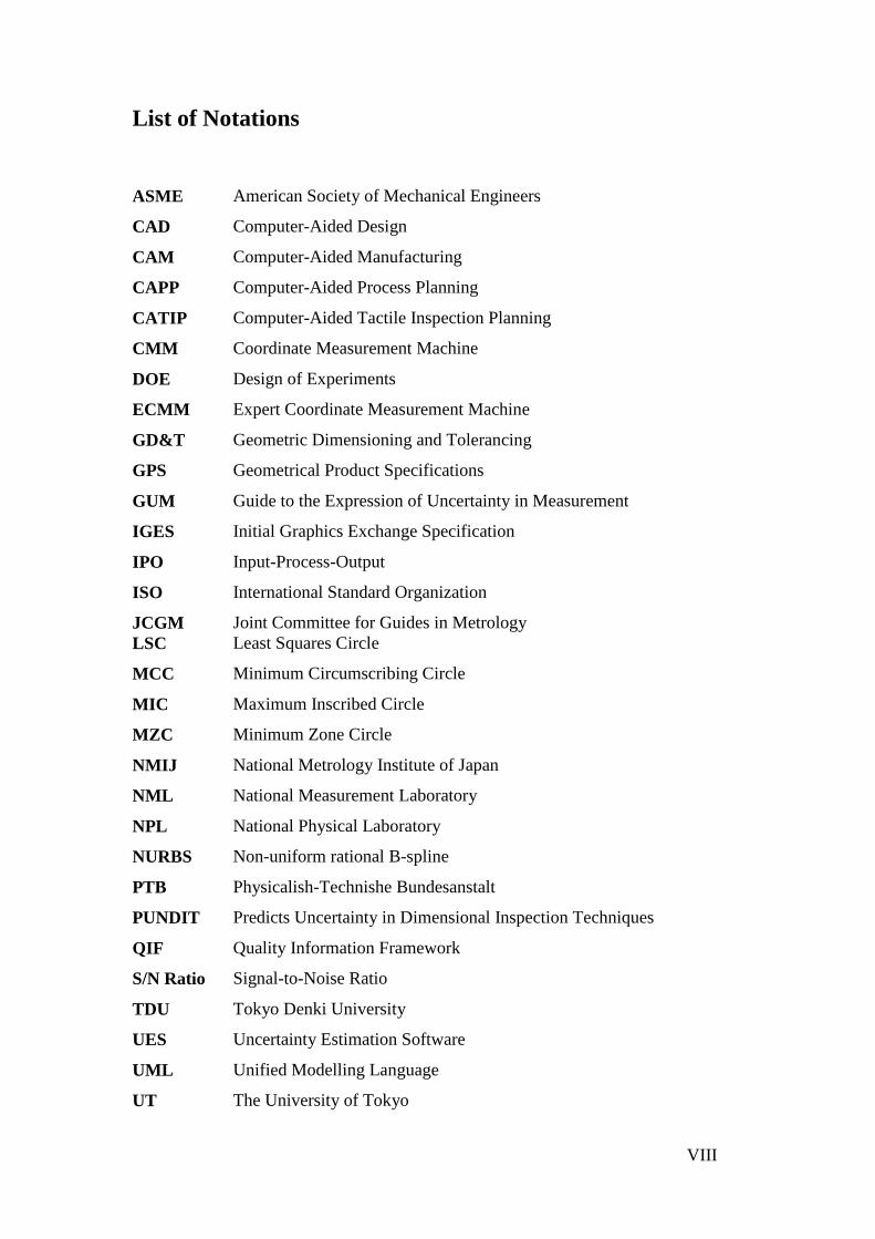
List of Notations

ASME American Society of Mechanical Engineers

CAD Computer-Aided Design

CAM Computer-Aided Manufacturing

CAPP Computer-Aided Process Planning

CATIP Computer-Aided Tactile Inspection Planning

CMM Coordinate Measurement Machine

DOE Design of Experiments

ECMM Expert Coordinate Measurement Machine

GD&T Geometric Dimensioning and Tolerancing

GPS Geometrical Product Specifications

GUM Guide to the Expression of Uncertainty in Measurement

IGES Initial Graphics Exchange Specification

IPO Input-Process-Output

ISO International Standard Organization

JCGM Joint Committee for Guides in Metrology

LSC Least Squares Circle

MCC Minimum Circumscribing Circle

MIC Maximum Inscribed Circle

MZC Minimum Zone Circle

NMIJ National Metrology Institute of Japan

NML National Measurement Laboratory

NPL National Physical Laboratory

NURBS Non-uniform rational B-spline

PTB Physicalish-Technishe Bundesanstalt

PUNDIT Predicts Uncertainty in Dimensional Inspection Techniques

QIF Quality Information Framework

S/N Ratio Signal-to-Noise Ratio

TDU Tokyo Denki University

UES Uncertainty Estimation Software

UML Unified Modelling Language

UT The University of Tokyo

IX

VCMM Virtual Coordinate Measurement Machine

VIM International Vocabulary of Metrology

X

List of Figures

Figure 1 Dimensional measurement instruments ........................................................... 3

Figure 2 Online measurement simulation software ....................................................... 4

Figure 3 Outline of the uncertainty calculation in GUM ............................................. 12

Figure 4 The basic concept of Monte Carlo Method ................................................... 13

Figure 5 Tolerance classification in GD&T standards ................................................ 15

Figure 6 Determine Volumetric Probing Error ............................................................ 22

Figure 7 Determine Volumetric Length Measuring Error ........................................... 22

Figure 8 Flowchart of the proposed feature-based inspection process planning

system…………………...............................................................................30

Figure 9. Fuzzy system structure to determine the number of measuring points. ....... 32

Figure 10 Areas where post-measurement data processing are served ........................ 36

Figure 11 Conclusion of CMM measurement planning and modelling ...................... 38

Figure 12. Measurement in digital and physical world ................................................ 40

Figure 13. The UES requirements specified in ISO 15530-4. ..................................... 41

Figure 14. Error components that lead to uncertainties ............................................... 43

Figure 15. The VCMM concept ................................................................................... 44

Figure 16. Overall scheme of the ECMM .................................................................... 46

Figure 17. Overall scheme of simulation-by-constraints method ................................ 48

Figure 19. The case study is an honourable corporation between three prestige

organizations. ................................................................................................. 59

Figure 20 Error sources considered in CMM modelling software .............................. 62

Figure 21 Operations flow . ......................................................................................... 63

Figure 22 Monte Carlo simulation applied to metrology ............................................. 64

Figure 23 CAD model of the complex product for the case study. ............................. 64

Figure 24 Points sampling of the oblique hole ............................................................ 66

Figure 25 Simulation Result ........................................................................................ 67

Figure 26 A representation of the gas turbine system .................................................. 70

Figure 27 A representation of the inspected part ......................................................... 71

Figure 28 A generic compontent input model ............................................................. 75

Figure 29 Comparison between physical measurement and simulation results........... 78

Figure 30 Uncertainty comparison between simulation result and GUM calculation . 83

XI

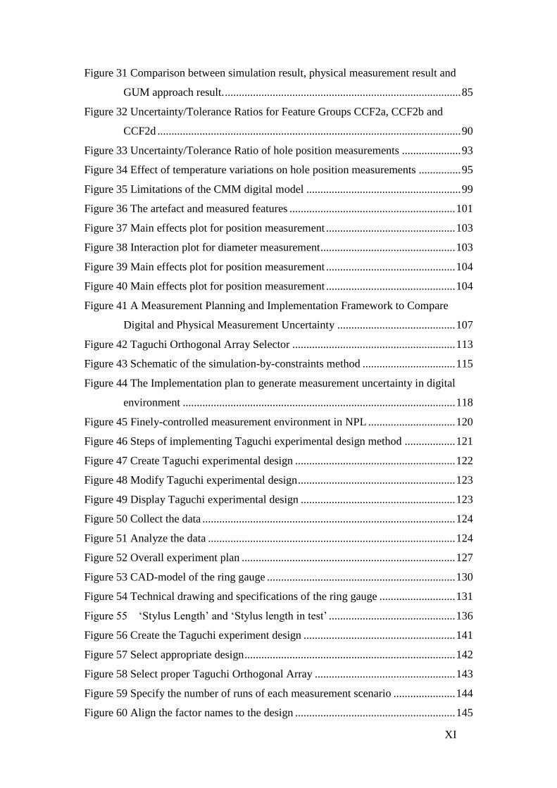
Figure 31 Comparison between simulation result, physical measurement result and

GUM approach result. .................................................................................... 85

Figure 32 Uncertainty/Tolerance Ratios for Feature Groups CCF2a, CCF2b and

CCF2d ............................................................................................................ 90

Figure 33 Uncertainty/Tolerance Ratio of hole position measurements ..................... 93

Figure 34 Effect of temperature variations on hole position measurements ............... 95

Figure 35 Limitations of the CMM digital model ....................................................... 99

Figure 36 The artefact and measured features ........................................................... 101

Figure 37 Main effects plot for position measurement .............................................. 103

Figure 38 Interaction plot for diameter measurement ................................................ 103

Figure 39 Main effects plot for position measurement .............................................. 104

Figure 40 Main effects plot for position measurement .............................................. 104

Figure 41 A Measurement Planning and Implementation Framework to Compare

Digital and Physical Measurement Uncertainty .......................................... 107

Figure 42 Taguchi Orthogonal Array Selector .......................................................... 113

Figure 43 Schematic of the simulation-by-constraints method ................................. 115

Figure 44 The Implementation plan to generate measurement uncertainty in digital

environment ................................................................................................. 118

Figure 45 Finely-controlled measurement environment in NPL ............................... 120

Figure 46 Steps of implementing Taguchi experimental design method .................. 121

Figure 47 Create Taguchi experimental design ......................................................... 122

Figure 48 Modify Taguchi experimental design ........................................................ 123

Figure 49 Display Taguchi experimental design ....................................................... 123

Figure 50 Collect the data .......................................................................................... 124

Figure 51 Analyze the data ........................................................................................ 124

Figure 52 Overall experiment plan ............................................................................ 127

Figure 53 CAD-model of the ring gauge ................................................................... 130

Figure 54 Technical drawing and specifications of the ring gauge ........................... 131

Figure 55 ‘Stylus Length’ and ‘Stylus length in test’ ............................................. 136

Figure 56 Create the Taguchi experiment design ...................................................... 141

Figure 57 Select appropriate design ........................................................................... 142

Figure 58 Select proper Taguchi Orthogonal Array .................................................. 143

Figure 59 Specify the number of runs of each measurement scenario ...................... 144

Figure 60 Align the factor names to the design ......................................................... 145

XII

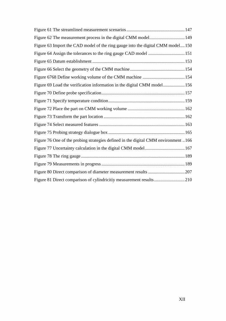
Figure 61 The streamlined measurement scenarios ................................................... 147

Figure 62 The measurement process in the digital CMM model............................... 149

Figure 63 Import the CAD model of the ring gauge into the digital CMM model .... 150

Figure 64 Assign the tolerances to the ring gauge CAD model ................................ 151

Figure 65 Datum establishment ................................................................................. 153

Figure 66 Select the geometry of the CMM machine ................................................ 154

Figure 6768 Define working volume of the CMM machine ..................................... 154

Figure 69 Load the verification information in the digital CMM model ................... 156

Figure 70 Define probe specification ......................................................................... 157

Figure 71 Specify temperature condition ................................................................... 159

Figure 72 Place the part on CMM working volume .................................................. 162

Figure 73 Transform the part location ....................................................................... 162

Figure 74 Select measured features ........................................................................... 163

Figure 75 Probing strategy dialogue box ................................................................... 165

Figure 76 One of the probing strategies defined in the digital CMM environment .. 166

Figure 77 Uncertainty calculation in the digital CMM model ................................... 167

Figure 78 The ring gauge ........................................................................................... 189

Figure 79 Measurements in progress ......................................................................... 189

Figure 80 Direct comparison of diameter measurement results ................................ 207

Figure 81 Direct comparison of cylindricitiy measurement results ........................... 210

XIII

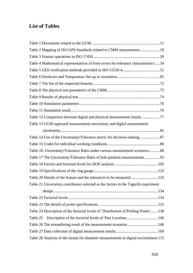
List of Tables

Table 1 Documents related to the GUM ...................................................................... 11

Table 2 Mapping of ISO GPS Standards related to CMM measurement .................... 18

Table 3 Feature operations in ISO 17450. ................................................................... 20

Table 4 Mathematical representatives of form errors for tolerance characteristics ..... 34

Table 5 UES verification methods provided in ISO 15530-4 ...................................... 51

Table 6 Hardware and Temperature Set-up in simulation ........................................... 65

Table 7 The list of the inspected features .................................................................... 72

Table 8 The physical test parameters of the CMM ...................................................... 73

Table 9 Results of physical test ................................................................................... 74

Table 10 Simulation parameters .................................................................................. 76

Table 11 Simulation result ........................................................................................... 76

Table 12 Comparison between digital and physical measurement results .................. 77

Table 13 GUM-approach measurement uncertainty and digital measurement

uncertainty ...................................................................................................... 82

Table 14 Use of the Uncertainty/Tolerance metric for decision-making..................... 87

Table 15 Codes for individual working conditions. ..................................................... 88

Table 16. Uncertainty/Tolerance Ratio under various measurement scenarios ........... 88

Table 17 The Uncertainty/Tolerance Ratio of hole position measurements ................ 93

Table 18 Factors and factorial levels for DOE analysis ............................................ 102

Table 19 Specifications of the ring gauge .................................................................. 132

Table 20 Details of the feature and the tolerances to be measured ............................ 132

Table 21 Uncertainty contributors selected as the factors in the Taguchi experiment

design ........................................................................................................... 134

Table 22 Factorial levels ............................................................................................ 134

Table 23 The details of probe specifications ............................................................. 135

Table 24 Description of the factorial levels of ‘Distribution of Probing Points’ ....... 138

Table 25 Description of the factorial levels of 'Part Location; ............................... 140

Table 26 The streamlining result of the measurement scenarios ............................... 146

Table 27 Data collection of digital measurement results ........................................... 169

Table 28 Analysis of the means for diameter measurements in digital environment 172

XIV

Table 29 Discussions of the control factor effects on diameter measurements in the

digital environment ...................................................................................... 175

Table 30 Analysis of the S/N ratios for diameter measurements in digital environment

...................................................................................................................... 176

Table 31 Analysis of the means for the cylindricity measurements in the digital

environment ................................................................................................. 178

Table 32 Discussions of the control factor effects on cylindricity measurements .... 181

Table 33 Analysis of the S/N ratios for cylindricity measurements in digital

environment ................................................................................................. 182

Table 34 Taguchi analysis result comparison between digital diameter measurement

and digital cylindricity measurement ........................................................... 184

Table 35 Available CMM machines in NPL ............................................................. 186

Table 36 Probe testing results .................................................................................... 187

Table 37 Physical measurement environment ........................................................... 188

Table 38 Probe used in the complementary study ..................................................... 190

Table 39 Measurement scenarios in the complementary study ................................. 190

Table 40 The measured features in the complementary study ................................... 191

Table 41 Data collection for physical measurement results ...................................... 192

Table 42 Analysis of the means for cylindricity measurements in physical environment

...................................................................................................................... 194

Table 43 Discussions of the control factor effects on diameter measurements in the

physical environment ................................................................................... 196

Table 44 Analysis of the S/N ratios for diameter measurements in physical

environment ................................................................................................. 198

Table 45 Analysis of the means for cylindricity measurements in physical

environment ................................................................................................. 200

Table 46 Analysis of the S/N ratios for cylindricity measurements in physical

environment ................................................................................................. 203

Table 47 Data collection for comparing diameter measurement results .................... 206

Table 48 Data collection for comparing cylindricity measurement results ............... 209

Table 49 Comparison of Taguchi analysis results of diameter measurements .......... 212

Table 50 Comparison of Taguchi analysis results of cylindricity measurements ..... 217

Table 51 L8 (2^7) Taguchi Orthogonal Array ........................................................... 230

Table 52 Example of Data Collection of Taguchi Experimental Design .................. 231

XV

Table 53 Example of Data Analysis of Taguchi Experimental Design ..................... 233

Table 54 Example of Analysis Result of Taguchi Experimental Design .................. 233

1

Chapter 1 Introduction

Dimensional Metrology is the science of calibrating and using physical measurement

equipment to quantify the physical size of or distance from any given object [1]. In

today’s global competitive market, high product quality becomes increasingly

important, and the accuracy assertion of the products becomes indispensable [2].

Consequently, dimensional metrology emerges as a critical step in manufacturing,

driving product development and quality control at steady and strong pace [3].

Improved measurement capability will open the door to significant productivity

benefits as improvements deliver.

Considerable progress has been made in dimensional measurement. In respect to

hardware, laser-based measurement instruments have been developed, allowing

measurement can be operated in contact, non-contact or hybrid manner. New

measurement technologies and techniques are continuously adopted by high-value

manufacturing line. In respect to software, measurement simulation packages are

created by using various simulation techniques. The measurement simulation package

can simulate the measurement process, and predict the measurement result. It allows

measurement operations executed in the digital environment, and therefore, save

financial and labour cost of executing physical measurements.

However, dimensional metrology still faces intense challenges to fulfil requirements

from high-value manufacturing. The practices of dimensional metrology are lack of

simplicity and standardization. Effective integration between digital and physical

measurement environments is not implemented. And measurement process

modelling has not been fully established.

In order to overcome these problems, a process model for measurement is imperative.

This process model should promote the integration between digital and physical

measurement environments, and release the potential of integrating measurement to

Product Lifecycle Management (PLM) system. In this thesis, attempts have been

towards this direction. A Measurement Planning and Implementation Framework has

been implemented to integrate digital and physical measurement environments, and a

2

metrology-based process modelling has been developed, in particular for coordinate

measurement machine (CMM).

In this chapter, the background of this research is presented in Section 1.1. Then the

overall aims of the research are described in Section 1.2. Finally, Section 1.3 gives an

organizational outline of the thesis.

1.1 Background

1.1.1 Metrology and measurement in high-value manufacturing

Global competition in high-value manufacturing requires high product quality and

product complexity. To realize a proper function of a complex part, a product designer

needs to assign sufficiently narrow tolerances to product features, while the

manufacturer needs to produce the part to fulfil design requirements [4]. To achieve

this goal, dimensional metrology becomes increasingly important.

Many world-leading high-value manufacturers have established the facilities and

resources for effective measurements. Metrology has been generally realized as a part

of manufacturers’ strategy to achieve standardised methods for producing and sharing

data around a global production network. The collection and analysis of measurement

data is expected to be integrated into a production system - speeding up the decision

making process and allowing changes to be made in real time wherever possible

[5]. The need to continually assess the validity of measurement data is emerging.

Measurement results are expected to be utilized in a more sensible manner [6].

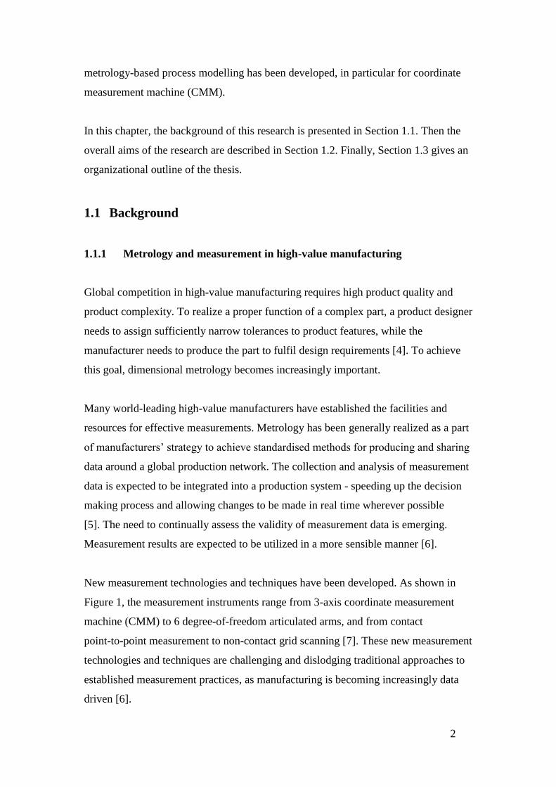
New measurement technologies and techniques have been developed. As shown in

Figure 1, the measurement instruments range from 3-axis coordinate measurement

machine (CMM) to 6 degree-of-freedom articulated arms, and from contact

point-to-point measurement to non-contact grid scanning [7]. These new measurement

technologies and techniques are challenging and dislodging traditional approaches to

established measurement practices, as manufacturing is becoming increasingly data

driven [6].

3

Figure 1 Dimensional measurement instruments

1.1.2 Measurement process modelling

In manufacturing, process modelling deals with determination of appropriate

operations and sequences to produce a tangible part from an engineering design [8].

With the booming development of computational techniques, the majority of process

modelling activities have been accomplished with the aid of digital environments [9].

Extensive research efforts have been made in process modelling, and have

demonstrated that process modelling is an effective and efficient technique for design

and manufacturing integration [10].

Measurement process modelling uses computational techniques to design, analyse and

optimize measurement processes. As metrology gets increasingly important in

high-value manufacturing, measurement process modelling becomes a key in

4

production efficiency improvement and cost reduction [6]. Proper measurement

process modelling can lead to a dramatic improvement in quality control and provide

smooth integration of product lifecycle management (PLM) [11].

Measurement process modelling could be generally categorized into three levels:

Direct measurement process modelling;

Measurement uncertainty estimation;

Robust measurement process modelling.

The details of these three levels are described in the following paragraphs.

Direct measurement process modelling

Direct measurement process modelling can be seen as an interface between physical

measurement operations and digital environment. As shown in Figure 2, features of

measurement instruments and measurement operations are established in direct

measurement process modelling. It visualizes physical measurement operations in

digital environment, collects measurement results and outputs these data to assist

product inspection and production quality control. Direct measurement process

modelling allows the realization of a physical measurement process in a digital

environment.

Figure 2 Online measurement simulation software

5

Measurement uncertainty estimation

Measurement uncertainty estimation considers measurement uncertainty* as a key

index of measurement process modelling. It allows end-users to configure

measurement scenarios in a measurement model, and employs sophisticated

quantitative analysis techniques to calculate task-specific measurement uncertainty

[12], the measurement uncertainty of a specific feature for the configured

measurement scenarios [13].

Process modelling for measurement uncertainty estimation allows knowing

measurement results priory to physical measurement results, and therefore saves

labour, time and resource cost from physical measurement operations [14]. Various

endeavours have been made to verify the performance of uncertainty estimation

models [15,16]. However, the verification work remains to be a challenge [17]. There

is an enormous diversity and complexity of measurement tasks. Controlling

uncertainty influence quantities in physical measurement is very expensive and

difficult. It is virtually impossible to replicate all of measurement tasks in physical

measurement environment.

Robust measurement process modelling

Robust measurement process modelling considers measurement as an essential

operation of product lifecycle, and therefore, aims to promote coherent integration of

measurement operation into product lifecycle.

Robust measurement process modelling is still at an early stage. One of the major

achievements is the introduction of the Qualify Information Framework (QIF) [18].

The QIF is an advanced measurement information-exchange platform, aiming to

provide seamless data transition between design, machining, measurement and quality

control. The genuine goal of the QIF is to enforce the total integration of PLM with

the aim of metrology operations [11]. Although the structures and the schemas of the

QIF are still under development, the QIF have shown promising prospect in terms of

* The details relating to measurement uncertainty can be referenced in Section 1.1.3.

6

manufacturing system integration. The proper adoption of the QIF will lead to the

standardization of measurement systems, and therefore greatly promote measurement

to integrate within manufacturing product lifecycle.

1.1.3 Measurement uncertainty and uncertainty analysis

Measurement uncertainty is the doubt that exists about the result of any measurement.

Since no measurement is entirely accurate, a statement of measurement uncertainty is

necessary to indicate the quality of measurement [19]. The fundamental concepts

relating to measurement uncertainty have been provided in the International

Vocabulary of Basic and General Terms in Metrology (VIM) [20] and the Guide to

the Expression of Uncertainty in Measurement (GUM) [21].

Given the high diversity and complexity of measurement operations, task-specific

measurement uncertainty has been introduced. Task specific uncertainty is the

measurement uncertainty associated with the measurement of a specific feature using

a specific measurement plan [13]. Task-specific measurement finely segments

complex measurement processes into manageable operations. The introduction of

task-specific measurement uncertainty allows the classification and standardization of

measurement processes, and consequently, enhances measurement process automation

and measurement system integration. In recent research, task-specific measurement

uncertainty has emerged as a key concept in coordinate measurement [22].

Various researches on measurement uncertainty analysis have been carried out, e.g.

conformance assessment [23], cost reduction [24] and risk management [25].

Enormous advances in computational science have made it feasible to deploy

sophisticated quantitative analysis techniques to measurement uncertainty analysis.

Measurement uncertainty analysis has gained increasing interests from academics and

industry. Refining methods of measurement uncertainty analysis are expected to speed

up the decision-making process in complex product manufacturing, and to improve

product verification capability and capacity in global supply chain [6].

7

1.2 Overall aims

The overall aims of this research are to develop generic methodologies for

measurement process modelling, and to integrate physical metrology systems within

the digital environment, allowing smooth integration between digital and physical

measurement environments.

The detailed aims and objectives will be discussed in Chapter 3.

1.3 Organization of the thesis

The thesis is organized in 8 chapters as follows:

In Chapter 1, the background related to this research is introduced and overall aims of

the research are given.

In Chapter 2, a review of the related research is discussed. Three topics that are

relevant to this research – coordinate measurement, computer-aided measurement

planning and modelling and evaluation of task-specific measurement uncertainty

using simulation, are reviewed.

In Chapter 3, the aims, objectives and the methodology of this research are given.

In Chapter 4, a pilot study on the digital measurement model is performed by carrying

out physical measurement on a realistic component in shop floor environment. From

the pilot study, the problems relating digital measurement verification are realized.

In Chapter 5, a Measurement Planning and Implementation Framework is proposed

aiming to integrate digital and physical measurement uncertainty by statistically

analysing task-specific measurement uncertainty.

8

In Chapter 6, the implementations of the Measurement Planning and Implementation

Framework are presented, and the corresponding verification work are planned and

carried out. The feasibility of the Framework is approved in a scientific manner.

Finally, Chapter 7 gives the conclusions and contributions to the knowledge of this

research. The suggestions for future work are also outlines.

9

Chapter 2 Literature Review

2.1 Fundamentals of coordinate measurement

2.1.1 Fundamentals of measurement uncertainty

The highest-level guidelines for all forms of metrology activities are constructed in

the International Vocabulary of Basic and General Terms in Metrology (VIM) [20]

and the Evaluation of Measurement Data - Guide to the Expression of Uncertainty in

Measurement (GUM) [21]. They provide the fundamentals of measurement and

measurement uncertainty. They aim to solve popular metrology issues, such as

traceability, accuracy, precision, uncertainty and error, etc. Since being drafted in

1997, the GUM and the VIM have been widely adopted by industrial applications and

in academia.

1) The International Vocabulary of Basic and General Terms in Metrology (VIM)

The VIM [20] provides the “basic and general concepts and associated terms” in

metrology. In the introduction, it is clarified that even the finest measuring process

cannot confirm the measuring result as a single true value. The objective of a modern

measuring process is to determine a set of information that contains an interval of the

measuring results and the deviation from this interval, named as “measurement

uncertainty”. The vocabularies in metrology are rigorously defined or precisely

described with detailed additional explanation. The VIM has defined critical

considerations on practicing a measurement activity as below [20]:

Measurement Result: set of quantity values being attributed to a measurand

together with any other available relevant information;

Uncertainty: non-negative parameter characterizing the dispersion of the

quantity values being attributed to a measurand, based on the information

used;

Error: measured quantity value minus a reference quantity value;

Accuracy: closeness of agreement between a measured quantity value and a

true quantity value of a measurand;

10

Precision: closeness of agreement between indications or measured quantity

values obtained by replicate measurements on the same or similar objects

under specified conditions;

Metrological traceability: property of a measurement result whereby the result

can be related to a reference through a documented unbroken chain of

calibrations, each contributing to the measurement uncertainty.

In the annex part of the VIM, a series of concept diagrams have been given to further

clarify the inter-relationships among the vocabularies and concepts.

2) The Evaluation of Measurement Data - Guide to the Expression of Uncertainty in

Measurement (GUM)

The GUM [21] provides general mathematical rules for computing the measurement

uncertainty. The GUM further developed the objective of measurement, that is “to

establish a probability that this essentially unique value lies within an interval of

measured quantity values, based on the information available from measurement”

[20].

Besides the main text of the GUM [21], under the banner of “Evaluation of

Measurement Data”, there are seven titles of the documents to further support or

explain the concepts in the GUM as listed in Table 1.

11

Table 1 Documents related to the GUM

Number Title Status

JCGM

100:2008

Evaluation of measurement data – Guide to the expression of

uncertainty in measurement [21] Approved

JCGM

104:2009

Evaluation of measurement data – An introduction to the "Guide

to the expression of uncertainty in measurement" and related

documents [26].

Approved

JCGM

101:2008

Evaluation of measurement data – Supplement 1 to the "Guide to

the expression of uncertainty in measurement" – Propagation of

distributions using a Monte Carlo method [27].

Approved

N/A Evaluation of measurement data – The role of measurement

uncertainty in conformity assessment. Being prepared

N/A Evaluation of measurement data – Concepts and basic principles. Being prepared

N/A

Evaluation of measurement data – Supplement 2 to the "Guide to

the expression of uncertainty in measurement" – Models with any

number of output quantities.

Being prepared

N/A Evaluation of measurement data – Supplement 3 to the "Guide to

the expression of uncertainty in measurement" – Modelling.

Early stage of

preparation

N/A Evaluation of measurement data – Applications of the

least-squares method. Early stage of

preparation

In JCGM100:2008, the main text of the GUM, it is re-enforced that the measurement

result is only complete if it provides an estimate of the quantity concerned (the

measurand interval) and a quantitative measure of the reliability of the estimate

(known as the uncertainty). In order to relate the input quantities (or uncertainty

sources) to generate a single measuring result, the GUM innovatively introduces a

GUM uncertainty framework [27]. It is a mathematical model where the uncertainty

and its components can be exactly computed by conceptualizing the standard

uncertainty, the combined standard uncertainty and the expand uncertainty, and by

utilizing the algorithms in the statistics and probability theorem, such as the

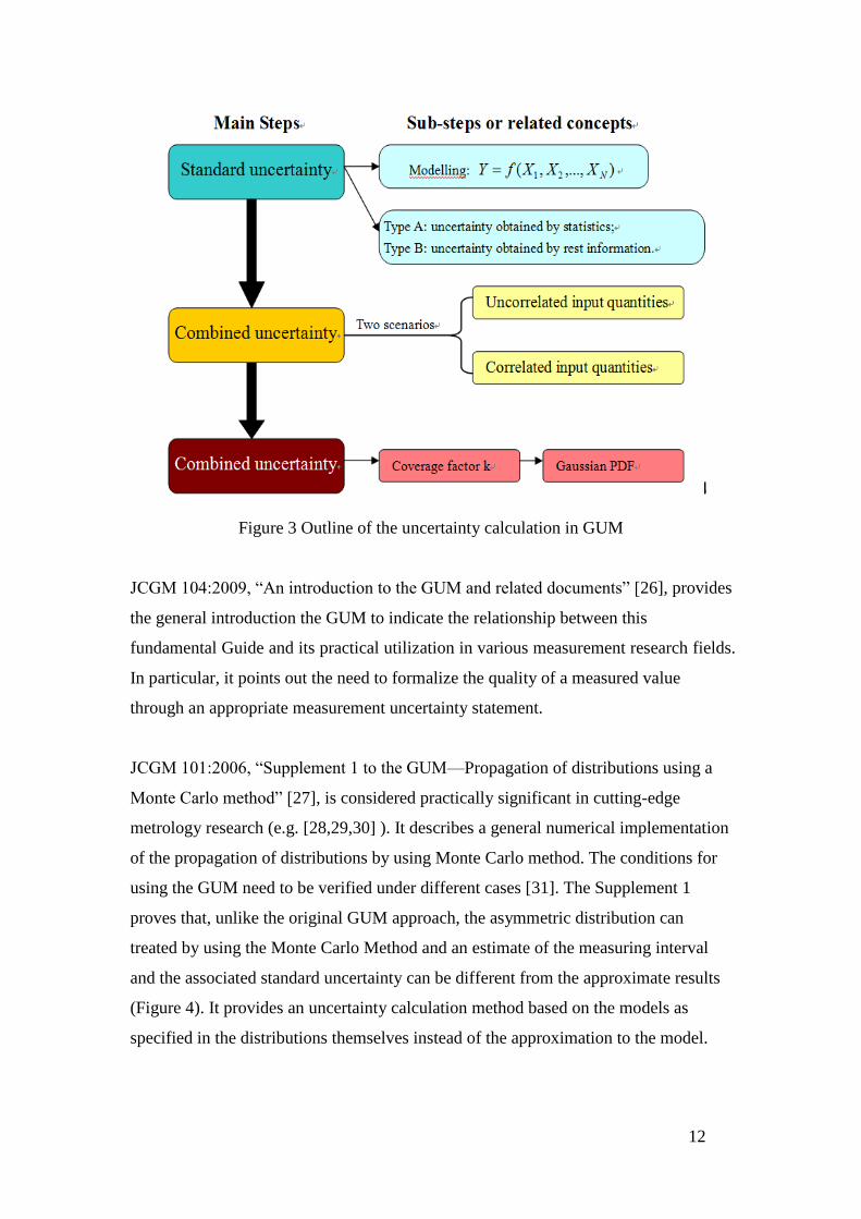
probability density function (PDF) and coverage factor (as outlined in Figure 3).

12

Figure 3 Outline of the uncertainty calculation in GUM

JCGM 104:2009, “An introduction to the GUM and related documents” [26], provides

the general introduction the GUM to indicate the relationship between this

fundamental Guide and its practical utilization in various measurement research fields.

In particular, it points out the need to formalize the quality of a measured value

through an appropriate measurement uncertainty statement.

JCGM 101:2006, “Supplement 1 to the GUM—Propagation of distributions using a

Monte Carlo method” [27], is considered practically significant in cutting-edge

metrology research (e.g. [28,29,30] ). It describes a general numerical implementation

of the propagation of distributions by using Monte Carlo method. The conditions for

using the GUM need to be verified under different cases [31]. The Supplement 1

proves that, unlike the original GUM approach, the asymmetric distribution can

treated by using the Monte Carlo Method and an estimate of the measuring interval

and the associated standard uncertainty can be different from the approximate results

(Figure 4). It provides an uncertainty calculation method based on the models as

specified in the distributions themselves instead of the approximation to the model.

13

Figure 4 The basic concept of Monte Carlo Method: The knowledge given to possible

values of each input quantity is expressed by a PDF and the knowledge of their

interrelationship with the values of the output quantity (measurand) by the model

function.

The rest of the GUM-related documents are not officially published yet. However, by

intensive literature review and closely following the current research in metrology,

concluding remarks can be conducted as below:

They extend the GUM in various ways, aiming to maintain a balance between

being updated with the current scientific advances and being stable as the

essential reference documents [32];

In “Evaluation of measurement data – Concepts and basic principle”, the

Bayesian probability theorem is proposed to provide a self-consistent method

permitting rigorous treatment of non-linear measurement models in

measurement data evaluation [32];

In “Evaluation of measurement data – The role of measurement uncertainty in

conformity assessment”, the problem of calculating the conformance

probability and the probabilities of the two types of error, given the

distribution, the specification limits and the limits of the acceptance zone is

addressed [33];

In “Evaluation of measurement data – Applications of the least-squares

method”, the guidance on the application of the least-squares method is

provided to data evaluation problems in metrology [34].

14

The topics in GUM supplements are abstracted from the latest research, of which

topics reflect the key trends in the metrology researches. But the current researches on

these topics are still unable to give a unified conclusion. There are challenges

remaining in metrology research, hence requiring to be further explored.

2.1.2 GD&T standards - ASME Y14.5M

Geometric Dimensioning and Tolerancing (GD&T) is a global engineering language

used in design, production and quality control. It is a system of symbols and

conventions used to specify the allowable limit of departure from the intended

geometry of a manufactured component. Primarily, it is aimed at ensuring

interchangeability. [35]. Today GD&T and the CMM are inseparably linked. It is

generally agreed that without the breaking-through invention of the CMM, efficient

inspection in accordance with its principles would be very much more difficult,

time-consuming and expensive.

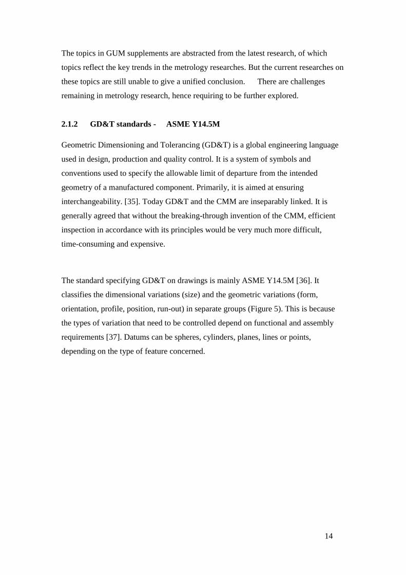
The standard specifying GD&T on drawings is mainly ASME Y14.5M [36]. It

classifies the dimensional variations (size) and the geometric variations (form,

orientation, profile, position, run-out) in separate groups (Figure 5). This is because

the types of variation that need to be controlled depend on functional and assembly

requirements [37]. Datums can be spheres, cylinders, planes, lines or points,

depending on the type of feature concerned.

15

Form

Straightens

Flatness

Roundness

Cylindricity

Profile

Any line on the surface must lie within a tolerance zone

formed by two parallel straight lines a distance t apart and in

the direction specified.

The surface must be contained within a tolerance zone

formed by two parallel planes a distance t apart.

The circumferential lie must be contained between a

tolerance zone formed by two coplanar concentric circles with

a difference in radii of t.

The cylindrical surface must be contained between a

tolerance zone formed by two coaxial cylinders with a

difference in radii of t.

The line or surface must be contained between a tolerance

zone formed by two lines or surfaces equidistant by t.

Orientation

Parallelism

Perpendicularity

Angularity

Profile

The line or surface must be contained between a tolerance

zone formed by two lines or planes a distance t apart and

parallel to the datum.

The line or surface must be contained between a tolerance

zone formed by two planes a distance t apart and

perpendicular to the datum.

The line or surface must be contained between a tolerance

zone formed by two planes a distance t apart at the specified

angle to the datum.

The line or surface must be contained between a tolerance

zone formed by two lines or planes a distance t enclosing the

theoretical profile relative to the datum(s).

Location

Position

Concentricity

Symmetry

Profile

The point, line or surface must be contained between a

tolerance zone form by a sphere or cylinder of diameter t, or

two planes a distance t apart, positioned as specified relative

to the datums.

The point or axis must be contained between a tolerance

zone formed by a circle or cylinder of diameter t concentric to

the datum

The surface must be contained within a tolerance zone

formed by two parallel places a distance t apart and which

are symmetrically disposed about the datum.

The line or surface must be contained between a tolerance

zone formed by two lines or surfaces equidistant by t

enclosing the theoretical profile relative to the datum(s).

Runout

Circular runout

Total runout

The line must be contained between a tolerance zone formed

by two coplanar and/or concentric circles a distance t apart

concentric with or perpendicular to the datum.

The surface must be contained between a tolerance zone

formed by tow coaxial cylinders with a difference in radii of t,

or planes a distance t apart, concentric with or perpendicular

to the datum.

Figure 5 Tolerance classification in GD&T standards (concluded from ASME Y14.5

Standard [36])

16

As stated in ASME Y14.5M, the original purpose of GD&T is to describe the

engineering intent of parts and assemblies [36]. Therefore, early research focussed on

practicing GD&T in tolerance analysis in order to sustain the part assembly and

functionality. As computer-added design (CAD) and computer-aided manufacturing

(CAM) were overwhelmingly adopted, considerable research efforts have been made

on extracting GD&T representations from CAD/CAM models and transforming the

tolerance analysis in a statistical way to govern manufacturing processes precisely

[38,39,40,41]. Shen et al. [42] proposed a semantic GD&T representation model,

named the “constraint-tolerance-feature-graph” that is claimed to satisfy all tolerance

analysis needs. Kong et al. [43] formulated an approach for the analysis of

non-stationary tolerance variation during a multi-station assembly process with

GD&T considerations.

Automated inspection is another area in which GD&T has been widely employed. By

properly executing GD&T methods, automated inspection systems can reliably and

effectively improve industrial manufacturing responsiveness, reduce the

time-to-market life cycle, and increase product competition [44]. Hunter et al [44]

established an approach to modelling and automating the part inspection process

design through the integration of part GD&T in a knowledge-based system (KBS).

Mohib et al [45] proposed a feature-based hybrid inspection planning, of which the

first step is to interpret the CAD models to gather the relevant design information and

GD&T specifications.

Since the development of non-contact scanning instruments, automated inspection

systems for 3-D scanning measurements have been increasingly focused. GD&T

analysis techniques are deployed in the 3-D scanning process. Prieto et al. [46,47]

implemented an approach to inspect free-form surface dimensional and geometric

tolerances using a set of 3D point clouds registered with a part CAD model and

verifying the specified tolerances. Son et al. [48] studied an automated inspection

planning system for free-form shape parts by laser scanning, which focused on

scanning orientation and path determination by recognizing GD&T representations.

Gao et al. [49] defined a Nominal Inspection Frame (NIF) for a nominal CAD model,

in which every GD&T specification may be defined and specified, particularly for

non-contact measurements.

17

To summarize, GD&T brings significant benefits to inspection activities. GD&T

representation ensures that the component parts can be assembled into final with the

intended functionality [36]. However, GD&T is sometimes mistakenly implemented

due to the misunderstanding on design process [50]. Moreover, it is common to

encounter the problems, e.g. lack of clarifying definitions in the feature locations, the

orientation controls, and the variation specifications [51]. Zhang et al [52] points out

that defining the GD&T requirements depends not only on capturing the functional

requirements, but also on the cost and quality issues, and this becomes an even more

challengeable element of the mechanical parts design. Maropoulos and Ceglarek [17]

conclude that the GD&T is not adjusted for measurability analysis, and is not

considered comprehensively for the planning of the measurement processes.

2.1.3 ISO GPS framework for CMM measurement

The original purpose of the ISO Geometrical Product Specification (GPS) framework

is the integration of design and manufacturing. A product representative language is

expected to be delivered in the ISO GPS framework to enable the communication

between design engineers and manufacturing engineers.

The British Standard BS8888 provides an overview of the ISO GPS framework [53].

It explains the concept of ISO GPS framework as [53]:

The GPS standards include several types of standards, dealing with the

fundamental rules of specification, global principles and definitions and

geometrical characteristics respectively;

The GPS standards provide several kinds of geometrical characteristics, such

as size, distance, angle, edge, form, orientation, location, roughness and

waviness;

The GPS standards define the workpiece characteristics as results of

manufacturing processes and specific machine elements;

The GPS standard can be applied at various steps of the product lifecycle,

including design, manufacturing, metrology and quality assurance.

However, the standards under the ISO GPS framework have been developed by

various ISO Technical Committees. There are still some standards missing or

incomplete [54].

18

Given the nature of this research, ISO 14660, ISO 17450, ISO 10360 and ISO 15530

are reviewed. The bibliographic details of the standards are listed in Table 2. The

contents of the standards are discussed individually in the following sub-sections.

Table 2 Mapping of ISO GPS Standards related to CMM measurement

Standard

No. Title Sub-Part No. Sub-Part title Year

BS EN

ISO 17450

General

concepts

BS EN ISO

17450-1:2011

Model for geometrical specification

and verification 2011

DD ISO/TS

17450-2:2002

Basic tenets,

specifications ,operators and

uncertainties

2002

BS EN

ISO 10360

Acceptance

and

reverification

tests CMM.

BS EN ISO

10360-1:2001 Vocabulary 2001

BS EN ISO

10360-2:2002 CMMs used for measuring size 2002

BS EN ISO

10360-3:2001

CMMs with the axis of the rotary

table as the fourth axis 2001

BS EN ISO

10360-4:2001

CMMs used in scanning measuring

mode 2001

BS EN ISO

10360-5:2001

CMMs using single and multiple

stylus contacting probing systems 2001

BS EN ISO

10360-6:2001

Estimation of errors in computing

Gaussian associated features 2001

DD CEN

ISO/TS

15530

Technique

for

determining

the

uncertainty

of

measurement

for CMM

DD CEN ISO/TS

15530-3:2007

Use of calibrated workpieces or

standards 2007

DD ISO/TS

15530-4:2008

Evaluating task-specific uncertainty

using Simulation 2008

1) ISO 17450 – General Concepts

ISO 17450 [55,56] is designated to provide concepts for the ISO GPS framework. It

aims to codify the geometric information of workpiece specifications in an

unambiguous fashion to integrate design, manufacturing and inspection.

A model for geometrical specification and verification is provided in ISO 17450 – 1

[55]. The fundamental concept is that a range of deviations of workpiece geometrical

specifications to be given to the workpiece’s function should be considered at the

product design stage. This design stage is named as ‘geometrical specification’, where

19

the geometrical information of the workpiece is specified and defined with tolerance

values. The verification procedure must start from the defined tolerances.

ISO 17450 [55, 56] develops a set of the terms and definitions to enable how well a

specification can express the workpiece function. To obtain ideal or non-ideal features,

ISO 17450 – 1 [55] concludes a series of specific operations as listed in Table 3.

20

Table 3 Feature operations in ISO 17450 (concluded from [55]).

Operation Description Example

Partition

A particular subset

of the real surface

is identified for

each surface to be

verified.

Extraction

A subset of the real

feature is

approximated using

a physical

extraction process

generating to a

finite set of point

this feature

operation

Filtration

The physical

extraction process

to reduce the

information of the

set of points to

describe only the

frequencies of

merit for the

verification of the

particular

surface-tolerance

combination.

Association

The filtered point

set is used to

estimate the closest

fitting substitute

geometry.

Collection

All the applicable

surfaces are

considered at the

same time, when

two or more

surfaces are

influenced by one

tolerance.

21

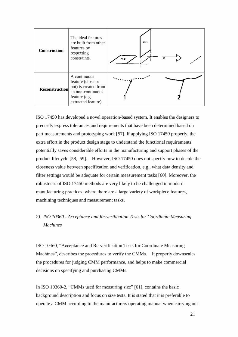
Construction

The ideal features

are built from other

features by

respecting

constraints.

Reconstruction

A continuous

feature (close or

not) is created from

an non-continuous

feature (e.g.

extracted feature)

ISO 17450 has developed a novel operation-based system. It enables the designers to

precisely express tolerances and requirements that have been determined based on

part measurements and prototyping work [57]. If applying ISO 17450 properly, the

extra effort in the product design stage to understand the functional requirements

potentially saves considerable efforts in the manufacturing and support phases of the

product lifecycle [58, 59]. However, ISO 17450 does not specify how to decide the

closeness value between specification and verification, e.g., what data density and

filter settings would be adequate for certain measurement tasks [60]. Moreover, the

robustness of ISO 17450 methods are very likely to be challenged in modern

manufacturing practices, where there are a large variety of workpiece features,

machining techniques and measurement tasks.

2) ISO 10360 - Acceptance and Re-verification Tests for Coordinate Measuring

Machines

ISO 10360, “Acceptance and Re-verification Tests for Coordinate Measuring

Machines”, describes the procedures to verify the CMMs. It properly downscales

the procedures for judging CMM performance, and helps to make commercial

decisions on specifying and purchasing CMMs.

In ISO 10360-2, “CMMs used for measuring size” [61], contains the basic

background description and focus on size tests. It is stated that it is preferable to

operate a CMM according to the manufacturers operating manual when carrying out

22

tests. Testing should also be done in conditions similar to those of the intended use.

The errors in CMM measurement are divided into two sets:

Volumetric Probing Error;

Volumetric Length Measuring Error.

Figure 6 Determine Volumetric Probing Error

Volumetric Probe error is caused when the CMM probe approaches the work piece

from different directions. As shown in Figure 6, to determine Volumetric Probe error,

25 point measurements are required to be made on the surface of a sphere, and then

the measurement results are computed to get the deviation of points from the Gaussian

associated sphere.

Figure 7 Determine Volumetric Length Measuring Error

Volumetric Length Measuring Error is the primary measure of the accuracy of a

CMM. As shown in Figure 7, to determine Volumetric Length Measuring Error, five

23

different calibrated lengths are placed in seven different locations and/or positions and

measured three times in each position for a total of 105 measurements.

ISO 10360-5, “CMMs Using Single and Multiple Stylus Contacting Probing

Systems”, covers the performance tests for contacting probing systems [62].

Volumetric Probing Error in ISO 10360-2 is taken out, and is integrated as ‘single

stylus probing system test’ in ISO 10360 – 5. Noticeably, probing system

performance is highly influenced by CMM performance. Probing system performance

cannot be isolated and tested as “stand-alone specification”. The tests procedures

specified in ISO 10360-5 are sensitive to many errors produced by the complex

“CMM” system. Therefore, in Annex B of ISO 10360-5, it is suggested to test

probing system performance prior to testing CMM performance.

ISO 10360 is developed for ‘standard’ Cartesian CMMs. But as non-Cartesian CMM

and optical systems gain more importance in applications, researchers have started to

re-assess the effectiveness of testing procedures in ISO 10360. Reference objects such

as step gauges can only be used for tactile photogrammetric systems which are

working similar to CMMs [63]. ISO 10360 does not consider triangulation systems.

Many optical systems are equipped by highly portable measuring sensors (e.g. camera

stations) and perform variable measuring accuracy under different scales and system

setups [64]. Extensive testing (as listed in ISO 10360) at the customer side brings up

some problems or obscurities in the requirement specifications [65]. But as ISO

10360 has been updated recently, a few researchers claimed that ISO 10360 allows

transferring test procedures to new measurement equipments based on an agreement

between supplier and CMM user [66].

3) ISO 15530 - Technique for Determining the Uncertainty of Measurement for

CMM

24

ISO 15530 deals with the general issues during CMM measurements tasks*. Major

parts of ISO 15530 are incomplete. One of the most referenced parts is ISO 15530 – 4,

Evaluating Task-Specific Measurement Uncertainty Using Simulation [67].

ISO 15530 – 4 aims to define the criteria for using computer simulation methods to

determine task-specific measurement uncertainties. Computer simulation methods are

expected to enable users to make quick judgements on the consistency of the

measuring process or to carry quick conformance assessments on the work piece as

required by ISO 14253 - 1.

ISO 15530 – 4 is the result of a long-term research focused on developing of Virtual

CMM, a simulation techniques applied to CMM measurement [13]. It proposes

three key concepts:

Uncertainty Evaluation Software (UES);

UES model and

UES validation [67].

The UES is software used to provide uncertainty evaluation by simulating the overall

CMM measuring process on a work piece. UES model is based on numerical

procedures to handle input quantities (e.g. CMM types, environmental conditions) and

to generate the measurement uncertainty. ISO 15530 – 4 provides two approaches

for UES validation: physical experimental validation on calibrated artefacts and

Computer-aided Verification and Evaluation (CVE).

At the time of writing the thesis, ISO 15530 - 4 is still in the first phase of the draft

status, which means it does not have the full status of an international standard. But

some researchers and software developers have already practiced ISO 15530 – 4 to

guide their CMM measurement simulation activities. Summerhays et al.[14]

developed a CMM measurement uncertainty prediction package, PUNDIT, given to

ISO 15530 requirements. Baldwin et al [15] presented several application examples to

demonstrate that simulation methods exhibit notable strength and versatility in

predicting CMM measurement uncertainty. Phillips et al. [22] compared two

commercially available UES, Virtual CMM and PUNDIT, and hence identified their

* This is the difference between ISO 15530 and ISO 10360. ISO 10360 is for judging CMM performance to serve

the decision-making on CMM selection.

25

advantages and disadvantages. However, the credibility of UES results remains

controversial. The study indicates the simulation results tend to be generally lower

than physical measurements [22]. Further refinements in UES and ISO 15530 – 4 are

necessary. Since ISO 15530 – 4 is designated for task-specific measurement

uncertainty, which “is the measurement uncertainty associated with the measurement

of a specific feature using a specific measurement plan [67]”, a universal UES, which

can comprehensively cover CMM measurement tasks, remains to be challenge to UES

developers and CMM measurement simulation researchers.

2.1.4 Summary

The fundamentals of measurement uncertainty have been introduced in the VIM and

the GUM, which aim to provide trustworthy guidance on metrology. The topics

discussed in the GUM supplements represent the latest focal points in measurement

uncertainty, e.g. conformity assessment, Monte-Carlo simulation method and

post-measurement data analysis. They have provided a platform to guide research on

using simulation techniques to predict measurement uncertainty, but these topics are

still under development. Therefore, simulation techniques based on the

VIM/GUM-approach need to be further explored and developed.

GD&T representation, ASME Y14.5M, ensures that component parts can be

assembled into final products and function as per the design intent. But it is

challenging to implement GD&T in a dual-communication manner, where both the

designer’s and manufacturer’s requirements are unambiguously represented. Crucially

to measurement and assembly, the GD&T is not adjusted for the measurability

analysis, and is not considered comprehensively for the measurement processes.

Therefore, simulation software based on GD&T concepts may not be able to interpret

the design intent and the manufacturing processes correctly or comprehensively.

The ISO GPS framework aims to provide a product representative language to enable

the tacit understanding between design and manufacturing. ISO 17450 [55, 56]

presents an approach to decoding the geometric information of workpiece

specifications in a fairly straightforward way, which has released the potential of

using simulation software to predict the manufacturing, inspection and measurement

26

results. ISO 15530 [67] has specifically explored how to evaluate task-specific

measurement uncertainty by using simulation software. The developments of the ISO

GPS framework have shed light on deploying simulation techniques for evaluating

CMM measurement uncertainty. However, as there may be a lack of consistency

between ISO GPS standards, the simulation algorithm developed under ISO GPS

standards should be used with considerable attention. Similarly, any simulation results

need to be verified and validated.

Conclusively speaking, the fundamentals for measurement uncertainty have been

developed and evolved. As theoretical attempts to defining measurement processes

and measurement uncertainty emerged, predicting measurement uncertainty in a

digital environment has become possible and popular. However, some inconsistencies

between the measurement standards inhibit the development of uncertainty evaluation

software (UES). The validation and verification of UES performance has become a

necessary and vital task for the UES developer and user.

2.2 CMM Measurement Planning and Modelling

CMM measurement planning is an essential part of the design and manufacturing

integration process [17]. It determines which features of a part to measure, what

resources are needed, and how to arrange the measurement procedures. It aims to

suggest the measurement strategy which achieves the desired measuring requirements

as well as consuming minimum measurement cost and time. Parts acceptance or

rejection is decided in the course of executing the measurement planning [68].

Therefore, CMM measurement planning has a significant effect on the product quality

and production time influencing cost and production profits.

Modern manufacturing is increasingly challenged by tight tolerances for producing

high quality and highly complex products. This leads to two major topics in CMM

measurement planning and modelling – automated measurement planning and online

measurement planning. Automated measurement planning provides accurate CMM

measurement models by using computer-aided support tools, assisting to make

decisions faster and better [68]. On-line measurement planning uses CMMs during the

machining process to achieve real-time production quality control rather than

27

acceptance or rejection of parts at the end. Many researchers in measurement planning

cover both of two topics, such as using computer-aided measurement planning for

online measurement. Given to the nature of the research, we focus on the review of

automated measurement planning [68].

Modern measurement process planning becomes a vital link to integrate design and

manufacturing [68]. Generally, recent research in this area is developed to accomplish

following the tasks:

Recognizing CAD models and features;

Optimizing inspection sequence;

Determining detailed measuring strategy (e.g. probe selection, number and

locations of measuring points, scanning speed);

Generating measuring paths;

Simulation and verification [69].

In terms of CMM measurement planning and modelling, the measuring stages are

generally defines as:

Inspection feature selection;

Inspection sequencing optimization;

Probing strategy determination;

Collision-free probe path generation;

CMM control command generation:

Post-measurement data processing, e.g. statistical cost analysis [70].

The recent measuring planning systems either covered all of the six stages, or focused

on accomplishing part of the stages.

2.2.1 Inspection feature selection

Feature selection and grouping is linked with feature recognition techniques in reverse

engineering where the CAD-models of parts are not available. Since the CAD-models

are usually available in CMM measurement planning, feature recognition is narrowed

to feature selection and grouping. Inspection features are the dimensions and

tolerances that have significant impact upon the parts’ functionalities [71]. The

purpose of feature selection and grouping is to determine which features are

necessarily to be measured, and to group them in preparation in the following steps of

28

measurement planning, e.g. inspection sequencing. On a traditional shop floor, the

selection and recognition of inspection features rely on the experiences of skilled

inspection engineers [68]. Early research either required manual input to specify the

inspection features, or automatically selected the inspection features only after

carefully monitoring the machining process. In contrast, recent research developed

feature selection techniques to the degree of full-automation. Inspection features can

be directly recognised/extracted from the CAD model. Most of the advances in feature

selection and grouping research happened not only in CMM measurement planning,

but also in on-line inspection planning using CMM or other measuring instruments.

Although the review was focused on CMM-based measuring planning, the research

reviewed CMM measurement planning to a more advanced level.

For CMM-based inspection planning, Zhang et. al [72] proposed a feature-based

inspection process planning system for CMM. To directly extract inspection features

from CAD models, the system sequentially undergoes five functional modules,

including tolerance feature analysis, accessibility analysis, clustering analysis, path

generation and inspection process simulation. Liamiem and ElMaraghy [73] proposed

a Computer-Aided Tactile Inspection Planning (CATIP) approach. Inspection features

are selected based from CAD model together with tolerance requirements, and

becomes the inputs of the system to optimize the inspection sequence. Hwang et al

[74] proposed a CMM inspection planning system, selecting inspection features based

on the tolerance specifications given by engineers.

Feature selection and grouping techniques for online measurement has made

significant advances. Wong et al. [75] proposed a feature recognition approach for

non-CMM inspection. This research classified the inspection features into seven

categories : (1) distance between two parallel faces which can be a length (e.g. width,

gap, slot, fin, height, protrusion, depth, recess or thickness, (2) diameter of a complete

cylinder/hole, (3) diameter or radius of a partial cylinder/hole or a cylindrical face, (4)

distance between a cylinder/hole and a parallel face, (5) distance between a pair of

cylinders/holes, (6) Coordinate measurement (or profile) measurement of a curved

surface (free-form or otherwise) with respect to a bounded reference plane, (7)

combination of the above. Based on the feature classification, a wide range of

29

measuring instruments could be selected. Lee et at. [76] proposed a two-stage

inspection process for the parts having many primitive features. The two stages are:

(1) Global inspection planning;

(2) Local inspection planning.

In Stage 1, the inspection features are selected by analysing features’ relations and

then grouped according to the extracted characteristics. In Stage 2, the features are

decomposed into their constituent geometric elements (e.g. plane, circle) for the

detailed measurement planning. Chung [77] developed an on-machining measurement

planning for free-form surfaces. The free-form features trimmed by NURBS are

translated by an IGES translator. The measurement codes are generated by means of

coordinate transformation and the uniform sampling software is linked with the IGES.

Cho and Seo [78] integrated the inspection process with the machining process by

analysing the machined surface errors. The geometrical form of the machined surface

is simulated in the system. Then the machining errors can be predicted by comparing

the simulated machined surface with the designed surface.

To conclude, latest research in feature selection and grouping has developed to the

automatic level by utilizing advanced digital engineering techniques. For CMM-based

measurement planning, inspection features are recognized and classified mainly on

the tolerance requirements. On-line inspection planning embraced diverse techniques

(e.g. feature grouping) and has made more advances. When a part is measured on the

same machining centre, the form of machining feature becomes more critical than the

tolerance value. Therefore online measuring planning used different techniques to

process the feature information and group them in another way.

2.2.2 Inspection sequence optimization

Optimizing the inspection sequences is closely linked with feature selection and

grouping in measurement process planning. Some recent research treated inspection

sequence optimization as part of feature selection and grouping, since features are

grouped under the consideration of optimizing the inspection sequence. The

sequencing of inspection features for CMM is mostly based on probe accessibility and

on minimizing probe orientations.

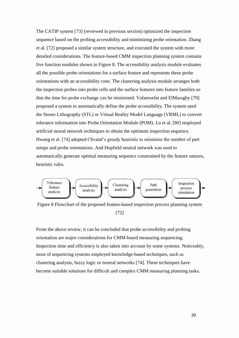
30

The CATIP system [73] (reviewed in previous section) optimized the inspection

sequence based on the probing accessibility and minimizing probe orientation. Zhang

et al. [72] proposed a similar system structure, and executed the system with more

detailed considerations. The feature-based CMM inspection planning system contains

five function modules shown in Figure 8. The accessibility analysis module evaluates

all the possible probe orientations for a surface feature and represents these probe

orientations with an accessibility cone. The clustering analysis module arranges both

the inspection probes into probe cells and the surface features into feature families so

that the time for probe exchange can be minimised. Vafaeesefat and ElMaraghy [79]

proposed a system to automatically define the probe accessibility. The system used

the Stereo Lithography (STL) or Virtual Reality Model Language (VRML) to convert

tolerance information into Probe Orientation Module (POM). Lu et al. [80] employed

artificial neural network techniques to obtain the optimum inspection sequence.

Hwang et al. [74] adopted Chvatal’s greedy heuristic to minimize the number of part

setups and probe orientations. And Hopfield neutral network was used to

automatically generate optimal measuring sequence constrained by the feature natures,

heuristic rules.

Figure 8 Flowchart of the proposed feature-based inspection process planning system

[72]

From the above review, it can be concluded that probe accessibility and probing

orientation are major considerations for CMM-based measuring sequencing.

Inspection time and efficiency is also taken into account by some systems. Noticeably,

most of sequencing systems employed knowledge-based techniques, such as

clustering analysis, fuzzy logic or neutral networks [74]. These techniques have

become suitable solutions for difficult and complex CMM measuring planning tasks.

31

2.2.3 Detailed probing strategy

Detailed sampling strategy mainly refers to topics relating to the CMM probe, e.g.

determining the measuring point density and distribution. The most common type of

CMM probe performs point-to-point contacting movements. Researchers focused on

minimizing the number of measuring points and measuring time as well as

maintaining measurement quality. The scanning probe collects sampling points by

continuous movement along the part surface, and hence shortens the inspection time.

As scanning probe technology matured, metrology researchers began to consider

including scanning probes in measurement planning and process.

Most research on point-to-point CMM measurement planning employed a

feature-based approach to determine proper measuring points. The density and

distribution of measuring points are decided for each measuring feature by

considering its tolerance value, geometric characteristics, and desired confidence level.

Huang et al. [81] proposed a knowledge-based inspection planning system for CMMs.

Part geometry, tolerance information and metrology expert knowledge were

considered together to determine the numbers and positions of measuring points. They

also applied their system to non-contact measuring systems. Cho et al [82] proposed a

fuzzy system for determining the optimum number of measuring points for the online

measurement system (Figure 9). The surface area, degree of tolerance and machine

accuracy were used as inputs into a ‘fuzzy system’. The Hammersley’s algorithm is

used to relocate the contacting measuring points on the target surfaces. Meanwhile,

the non-contact measuring points are generated by relocating the measuring points.

32

Figure 9. Fuzzy system structure to determine the number of measuring points [82].

The effect of selecting a particular sampling strategy has been recognized as a major

component of measurement uncertainty [83]. This effect is caused by the systematic

and random errors built-in the measurement systems [83]. Therefore, the CMM

measurement errors were usually categorised into two sets, systematic error and

random error, and the sampling strategy is optimized to reduce the two sets of errors

using statistical methods. Dowling et al. [84] addressed statistical issues in

feature-based measurement planning using CMM. The orthogonal least squares and

minimum-zone methods were used to evaluate the measuring deviation for a specific

feature. Jiang and Chiu [85] developed a statistical method for the determination of

the number of measurement points for 2D rotational part features. But Elkott et al. [86]

argued that research working on free-form feature measurement usually required large

sample sizes to inspect free-form features, and did not adequately explore how to

optimize the location of the measuring points. On the other hand, Zhao et al. [68]

claimed that these shortcomings can be solved by a hybrid measurement system,

which can automatically select a sampling algorithm that best fits the inspection

surface.

Abundant attempts have also been made to find a suitable sampling strategy for form

error evaluation. Form errors are the feature form deviations of a part resulting by the

combined effect of all the error sources in a real manufacturing environment.

Giovanni et al. [87] described form errors as ‘manufacturing signatures’, and tackled

33

the problem of determining sampling strategy starting from the characteristics of a

surface which is attributable to the manufacturing methods. Cui et al. [88] concluded

the mathematical representatives of form errors for various tolerance characteristics

(Table 4). There are four form error evaluation methods frequently used, which are,

least squares circle (LSC), minimum zone circle (MZC), maximum inscribed circle

(MIC), and minimum circumscribing circle (MCC). Chan et al. [92] studied the

influence of a number of points with equidistant sampling on the least square

parameters of a circle. Liu et al. [89] have studied the effect of CMM measurement

error on form tolerance using least squares and minimum zone methods. It is reported

that the Taylor sensitivity coefficients were obtained by regression, but the procedure

is not clearly described. Odayappan et al. [90] have studied the effect of sampling

strategies for circles. They have given recommendations for the minimum number of

points that have to be sampled for establishing the MZC, LSC, MCC and MIC. Cui et

al. [88] assessed the measurement results by using different form error evaluation

methods against CMM sampling. Some of the form error evaluation methods were

proposed particularly for circular features [91,92]. But now research was also

extended to free-form features [93,94].

34

Table 4 Mathematical representatives of form errors for tolerance characteristics [88]

Besides point-to-point measurement, the CMM scanning probe is attracting attention

from academia as its technology matures. Complete characterization of scanning

probe performances under various working conditions is in demand but still remains

unexplored. Moreover, the emergence of a scanning probe adds extra options for

CMM probe selection. Selecting the right type of CMM probe poses another

challenge for CMM measurement planning.

2.2.4 Probing path generation

The research in probing path generation focused on automatically generating

collision-free probing path when carrying out CMM measurement tasks.

Lu et al. [95] proposed an algorithm which uses a modified 3D octree ray tracing

technique to search for the colliding obstacles in an octree database on a selected path.

It also uses the global information about the obstacle vertices to reduce the zigzag

nature of the path generated by the octree based methods. Albuquerque et al. [96]

developed a collision-avoidance CMM inspection planning approach by defining the

relationships between features and configuring the tolerance types. This research

35

considered mainly circular and prismatic features. Ainsworth et al. [97] developed a

probe path generation system for free-form features. NURBS definition method was

adopted to mathematically represent the shape of a free-form surface. The probing

path was then generated through three stages: initial path generation, modification and

verification. They defined the probing movement as either uni-directional or

bi-directional. The implemented path planning software initially generates a

measurement path for each selected entity, based on the CAD model. The system also

allows users to modify the probing path parameters interactively. The final probing

path is processed into machine executable programming code. They used a turbine

blade which has an aerofoil shape to demonstrate their path generation system. Lin

and Murugappan [98] proposed an approach for automatically generating a CMM

probing path. It is assumed that the CMM probe is a point object. This assumption

simplifies the detection of collision into a single point and the part and fixtures are not

considered in this research.

To conclude the above review section, CMM probing path planning focuses on

automatically generating an optimum collision-free path. Graphic representation

methods are usually employed to recognise the feature shape, and hence to generate

the probing points and trigger the probing movements. Usually there is a verification

module, where the probing movements could be simulated in the digital environment;

therefore the automatically generated probing path could be verified.

2.2.5 Post-measurement data processing

After the CMM completes its physical measurements, the measurement results

collected from the parts are processed. This procedure is usually regarded as

‘post-measurement data processing’. It addresses data analysis techniques which can

improve the quality of the CMM measurement results. There are several broad types

of post-measurement processing objectives, such as to enhance the accuracy, to filter

the measurement ‘noise’ and to reduce the volume of measurement data collection.

Generally, the techniques for post-measurement processing are deployed in two

domains, design and production as shown in Figure 10. In the design domain,

post-measurement data are processed to serve reverse engineering. In the production

domain, post-measurement data are processed for quality control or cost analysis.

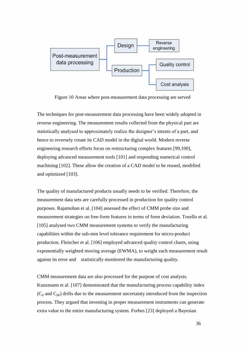
36

Figure 10 Areas where post-measurement data processing are served

The techniques for post-measurement data processing have been widely adopted in

reverse engineering. The measurement results collected from the physical part are

statistically analysed to approximately realize the designer’s intents of a part, and

hence to reversely create its CAD model in the digital world. Modern reverse

engineering research efforts focus on restructuring complex features [99,100],

deploying advanced measurement tools [101] and responding numerical control

machining [102]. These allow the creation of a CAD model to be reused, modified

and optimized [103].

The quality of manufactured products usually needs to be verified. Therefore, the

measurement data sets are carefully processed in production for quality control

purposes. Rajamohan et al. [104] assessed the effect of CMM probe size and

measurement strategies on free-form features in terms of form deviation. Tosello et al.

[105] analysed two CMM measurement systems to verify the manufacturing

capabilities within the sub-mm level tolerance requirement for micro-product

production. Fleischer et al. [106] employed advanced quality control charts, using

exponentially weighted moving average (EWMA), to weight each measurement result

against its error and statistically monitored the manufacturing quality.

CMM measurement data are also processed for the purpose of cost analysis.

Kunzmann et al. [107] demonstrated that the manufacturing process capability index

(Cp and Cpk) drifts due to the measurement uncertainty introduced from the inspection

process. They argued that investing in proper measurement instruments can generate

extra value to the entire manufacturing system. Forbes [23] deployed a Bayesian

37

decision-making approach to examine the measurement uncertainty impacts from the

economical perspective, and optimized the decision-making on rejecting or accepting

a part. The mathematical approach originated from the aero-engine shaft inspection,

where the shaft tolerances on radius and form error were inspected using a CMM.

Pendrill [108] developed a measurement uncertainty optimization model to balance

the testing costs and the cost associated with the consumer’s risk. Baldwin et al. [25]

proposed a CMM cost analysis approach by incorporating Taguchi Loss Function.

Despite of the above endeavours, research regarding the measurement cost and benefit

analysing is insufficient. It would be helpful if the measurement benefits could be

quantified, and could be demonstrated through focused research projects.

To conclude, post-measurement data processing is extensively adopted in reverse

engineering and quality control. The data collected by CMM measurements is usually

statistically processed in order to re-construct the parts’ CAD model or finely control

the production process. Recent research started to explore economical benefits by

statistically analysing the post-measurement data. But few of the approaches have

been progressed to focused research outcomes.

2.2.6 Summary

CMM measurement planning and modelling has been researched for decades. Recent

CMM measurement planning has achieved significant improvements with the

development of computer-aided design (CAD) and manufacturing (CAM)

technologies. As shown in Figure 11, the research is assigned to solve the problems in:

(1) inspection feature selection, (2) inspection sequencing optimization, (3) probing

strategy determination, (4) probing path generation (5) CMM servo control, and (6)

post-measurement data processing.

38

Scanning speed

Operation temperature

Maximum extension

Stylus length

Accuracy

Tolerance values

Factual ResourcesStages for CMM

measurement planning Reasoning algorithms

Inspection sequencing optimization

Feature accessibility

assessment

Probe orientation optimization

Detailed probing strategy

Point-to-point measurement

Scanning measurement

Number of measuring points

Distribution of measuring points

Probe selection (point-to-point

vs. scanning)

Scanning speed

Scanning trajectory

Collision-free probing path

generation

CMM control commands

generation

Post-measurement

data processing

Reverse engineering

Quality control

Cost analysis

Feature

characteristics

Heuristic resourcesFeature-based

CAD-model design

Standard feature

information

Standard feature

database

Standard

measurement

operation

Geometry

information

Tolerance

valute

Probe

information

Probe selection

Probe

orientaion

Number and

distribution of

sampling points

Probing paths

Measurement

sequence

optimization

Scanning

speed and

trajectory

Machining

information

Sensing direction

Inspection feature selection

Tolerance grade classification

Feature grouping

Feature relationship

identification

Working volumeWorking volume

ASME Y14.5M-

1994

GD&T design

standard

ISO 14253

ISO 10360

ISO CMM

verification standard

e.g. NPL Best Practices

Firmly-defined

Industrial best

practices (optional)

Gantry structure

CMM specification

(optional)

Knowledge-

based artificial

intelligence (AI)

techniques

Clustering

analysis

Fuzzy logic

Neutral

network Accuracy

Probe specification

Artificial

intelligence

techniques

Conformance assessment

Acceptance/Rejection decision-

making

Risk sharing between consumer

and producer

Figure 11 Conclusion of CMM measurement planning and modelling

39

Feature-based measurement planning has become the focus of recent research.

Standard Feature Database*, which documents standardized measurement operations

for each specific feature, have been proposed by various researchers. Due to the

high complexity of CMM measurement planning, knowledge-based artificial

intelligent techniques (e.g. clustering analysis, fuzzy logic) are frequently used to

generate proper measurement strategies from a Standard Feature Database. Although

Standard Feature Database poses certain challenges in real production practices, the

concept itself remains an optimistic solution which is able to deliver real efficiency

improvements for future CMM measurement planning.

Post-measurement data processing† has been developed. Measurement data sets are

statistically processed to serve the requirements from reverse engineering, quality

control and cost analysis. This introduces new research topics, e.g. conformance

assessment, decision-making under uncertainty and risk sharing. Further explorations

are still required in the post-measurement data processing area.

* As shown on the left-hand side of Figure 11.

† As highlighted in dark-blue in Figure 11.

40

Figure 12. Measurement in digital and physical world [1]

To conclude, as CMM technologies and techniques are getting highly advanced,

CMM measurement planning evolves as a necessary link to integrate design and

manufacturing. As shown in Figure 12, measurement becomes integral to

manufacturing processes, linking digital and physical worlds and interacting within

the phases of design and manufacturing integration process. But its development in

terms of measurement modelling and planning is embryonic when compared to

processes and additional research is needed in CMM measurement modelling and

planning.

41

2.3 Evaluation of task-specific measurement uncertainty using

simulation

2.3.1 Requirements of uncertainty evaluating software (UES) as specified in

ISO standard

The requirements for developing uncertainty evaluating software (UES) have been

informatively specified in ISO 15530-4 [67], “Evaluating Task-Specific Measurement

Uncertainty Using Simulation”.

E.g.

which CMM errors are

accounts for;

the types of CMMs for which

the software is applicable.

Claimed scope

E.g.

the geometrical deviations of the

CMM;

deviations of the probing system;

temperature gradients.

Uncertainty contributors accounted

by the UES

E.g.

CMM type;

CMM calibration test result;

CMM MPE value;

Operator effect.

UES inputs

E.g.

how the influence quantities are varied;

how the uncertainties are derived from

the simulated samples.

Additional documents

GUMSimulation

result

Figure 13. The UES requirements specified in ISO 15530-4 (concluded from [67]).

As shown in Figure 13, ISO 15530 – 4 claims that UES developers need to provide ‘a

claimed scope’ of the UES (including specifying uncertainty contributors taken into

account), the input quantities of the UES and additional documents involved to

support the UES development. Meanwhile, ISO 15530 – 4 points that all of the

statements provided by the UES developers need comply with GUM principles, and

the UES results need to be consistent with the ‘claimed scope’ initially provided by

the UES developer.

ISO 15530 – 4 provides a detailed checklist of the measurement uncertainty

contributors for CMM measurement. The UES developers are suggested to reference

42

the checklist to identify the key influence factors in defining the ‘claimed scope’ of

UES.

ISO 15530 – 4 points out that there can be two types of UES:

Online UES – where the simulation is integrated into a specific CMM

machine;

Offline UES – where the simulation is implemented as an independent system

on an external computer.

ISO 15530 – 4 describes the flowchart of the UES algorithm, which starts from a

specific measurement task, and then mathematically calculates the measurement

uncertainty taking into account the uncertainty contributors to the CMM measuring

process. The mathematical method to determine the task-specific measurement

uncertainty is also stated in the standard.

ISO 15530 – 4 has proposed the concept of Uncertainty Simulation Software (UES),

and informatively specifies the requirements for the UES development. The special

concerns in ISO 15530 -4 underline a key trend in computer-aided inspection - using

the simulation method to determine task-specific measurement uncertainty. However,

the comprehensiveness of the simulation method, e.g. considering all of the

measurement uncertainties during the simulation process, is virtually impossible to

achieve. The verification and validation of UES result is doubted by the final users of

the UES.

2.3.2 The simulation methods for evaluating task-specific measurement

uncertainty

The review paper [13] concerning task-specific measurement uncertainty has

identified error components that may lead to the measurement uncertainties (Figure

14), and concluded six methods for evaluating task-specific measurement uncertainty,

which are ‘sensitivity analysis’, ‘expert judgement’, ‘experimental method using

calibrated objects’, ‘computer simulation’, ‘statistical estimations from measurement

history’, and ‘ hybrid methods’. Various research efforts [12,109,110] have indicated

that the main flexible method for determining the uncertainty is the computer

simulation method.

43

Figure 14. Error components that lead to uncertainties

The computer simulation method offers the potential to configure highly complicated

CMM error models to the specific measurement task under consideration [15].

Various computer simulation packages have been developed, such as “Virtual CMM”

[111], “PUNDIT/CMM” [112], and “Expert CMM” [113]. Most of the methods work

on the basis of propagating uncertainty from the different sources to the measurement

results, but may operate in a slightly different approach.

A) The virtual CMM (VCMM)

The virtual coordinate measuring machine (VCMM) estimates task specific

measurement uncertainty for a specific CMM machine. The process starts by

assigning virtual probing points to an ideal geometry that represents the design

specification. At each probing point on a particular feature, the VCMM generates a

perturbed point [114]. The perturbed point is generated by modelling variations

coming from the different contributors to the measurement task. Each contributor is

simulated using a probability density function (PDF) and each perturbed point is

simulated by combining the information from all input contributors (PDFs).

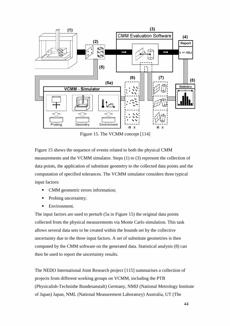
44

Figure 15. The VCMM concept [114]

Figure 15 shows the sequence of events related to both the physical CMM

measurements and the VCMM simulator. Steps (1) to (3) represent the collection of

data points, the application of substitute geometry to the collected data points and the

computation of specified tolerances. The VCMM simulator considers three typical

input factors:

CMM geometric errors information;

Probing uncertainty;

Environment.

The input factors are used to perturb (5a in Figure 15) the original data points

collected from the physical measurements via Monte Carlo simulation. This task

allows several data sets to be created within the bounds set by the collective

uncertainty due to the three input factors. A set of substitute geometries is then

computed by the CMM software on the generated data. Statistical analysis (8) can

then be used to report the uncertainty results.

The NEDO International Joint Research project [115] summarises a collection of

projects from different working groups on VCMM, including the PTB

(Physicalish-Technishe Bundesanstalt) Germany, NMIJ (National Metrology Institute

of Japan) Japan, NML (National Measurement Laboratory) Australia, UT (The

45

University of Tokyo) Japan and TDU (Tokyo Denki University) Japan. A discussion

[116] of how the VCMM concept could be generalised together with a general

methodology to take into account prior calibration information in uncertainty

estimation was also proposed by the NPL (National Physics Laboratory). Other

VCMM have been developed [117,118] to include enhanced user interfaces and 3D

simulation of the specific measurement task.

Several researchers have pointed out the disadvantages of VCMM. Firstly, VCMM

relies heavily on the accuracy of the CMM geometric description [119,120].

Secondly, the VCMM inputs (uncertainty associated with each contributor) need to be

assessed completely, but some of them cannot be economically measured or be easily

estimated. Thirdly, some essential uncertainty contributors (e.g. form error,

cleanliness, fixturing variability and operators) are not taken into account in the

VCMM approach [121,122].

B) The expert CMM (ECMM)

The Expert CMM project (ECMM) consisted of a collaboration between a national

metrology institute and industry [114]. The ECMM is a GUM-consistent UES

package dealing with task-specific measurement uncertainty. The ECMM developer

claims that ECMM requires minimum involvement of the user, and is capable to work

both online (for real-time inspection) and off-line (for alternative procedure

comparison). The ECMM keeps uncertainty contributors (e.g. CMM machine,

environment, workpiece) in separate groups, so it is easy to trace poor measurement

accuracy.

The ECMM method considers individual points of the measurand instead of

compound geometric features (e.g. diameters and angles), which is a breakthrough for

evaluating measurement uncertainty. The overall scheme of ECMM is shown in

Figure 16. The ECMM method assumes that the outputs, y, of the measuring system

are related to the inputs, x, through a transfer function, h(x). Nominal measurement

points, x0, are perturbed with errors from an error simulator using a Gaussian

pseudo-random number generator. The various simulated points are then fed through

46

the CMM software to produce a variety of outputs, y, which are statistically evaluated

to compute the variance covariance matrix to produce a complete uncertainty

statement as requested in GUM [21].

Figure 16. Overall scheme of the ECMM [12]

Testing of the ECMM has been done on a plate with two holes (60 mm and 20 mm in

diameter, 60 mm apart). The plate was measured in 100 positions and the length and

its uncertainty computed. In 89% of the cases the calibrated length was within the

computed uncertainty with a coverage factor of 2. Only geometric errors were used as

input factors during the ECMM simulation due to the fact that the machine was

47

located in a laboratory environment. The initial testing result is considered to be

successful [12].

C) Simulation-by-constraints

The simulation-by-constraints method [112,14] generalizes the VCMM simulation

concept, and allows the calculation of task-specific measurement uncertainty based on

standardized performance data, e.g. ANSI B89.4.1 CMM performance specifications

[123]. The overall scheme is illustrated in Figure 17.

The simulation-by-constraints method treats performance tests specifications as

mathematical constraints on the infinite number of possible virtual CMM states, each

of which is defined by specific parametric errors. These constraints, together with

reasonable assumptions (e.g. the CMM kinematic error model), greatly limit the

number of permissible states that the CMM may occupy. For example, the ANSI

B89.4.1 Standards provide volumetric performance test data for CMM. It includes the

measurement of ball bar lengths near the extremes of the CMM work zone. This is, in

effect, a boundary condition on the allowed parametric error functions. In order to be

self-consistent, the constrained parametric errors (e.g. the permissible virtual CMM

states) must faithfully reproduce the original performance specifications when a

simulation of the performance test is computed. Standard specifications provide

sufficient constraints to allow a reasonable calculation of task-specific uncertainty.

48

Figure 17. Overall scheme of simulation-by-constraints method

The simulation-by-constraints method does not require a full parametric error

description of the CMM machine, which is a major difference between the previously

described simulation methods*. The inspection engineers can use the

simulation-by-constraints results as the guidance for setting up a practical CMM

strategy as well as avoiding the need to physically error map all of the CMMs, which

is an expensive and impractical activity for industry.

A comparison between the VCMM method and the simulation-by-constraints method

[124] found that both methods approximated the experimental uncertainty values

calculated from the physical measurements of two ring gauges. The main difference

between the two methods is that the VCMM was likely to have a better description of

the machine geometry when compared with the MPE values used to describe the

machine geometry in the simulation-by-constraints method.

D) Hybrid approach

There are several approaches in the literature where researchers mixed the simulation

methods described above to address the task-specific measurement uncertainty

[125,126]. Generally, the hybrid approach employs the Monte Carlo technique to

generate the errors of each single measured point, and then uses the CMM

* Both of VCMM and ECMM require the assessment of the individual parametric errors of the CMM.

49

measurement program itself to propagate the measurement uncertainty. In the hybrid

approach, the CMM is not modelled, but its role in the measurement uncertainty

evaluation is emphasized as in the simulation-by-constraint method. The hybrid

approach provides an approximate yet reasonable evaluation of CMM measurement

uncertainty. Therefore it is supposed to fit an industrial production environment more

than a calibration laboratory.

Conclusively speaking, the simulation techniques for evaluating task-specific

measurement uncertainty have been developed for years. Nearly all of the simulation

techniques have been claimed to be consistent with GUM, while different simulation

methods require different accuracy levels of simulation parameter inputs. The more

accurate the simulation parameter inputs (e.g. a full error model of CMM machine)

fed to the simulation algorithm, the more accurate simulation result will potentially be

provided. But it is costly to determine an extreme accuracy description of simulation

parameters. Research is needed to scientifically explore the balance between the

accuracy of simulation parameter description and the simulation result.

Furthermore, due to the large versatility of CMM measurement tasks and inspected

features, it is virtually impossible to include all of the measurement uncertainty

contributors into the simulation algorithm. For example, it is hard to mathematically

define the interactions between the form error and the probing strategy, and hence it is

difficult to develop a fitting algorithm taking into account of form error.

2.3.3 The verification of UES performance

The computer code of the UES is not often disclosed by the UES developer, making it

difficult for the UES user to assess the reliability of the calculated uncertainty

statements. For a UES user, it is very important to verify the UES performance before

purchasing the software package. A set of UES verification procedures, which are

able to quantify the UES capability, would be of interest to both the UES developer

and the UES user.

The ISO 15530-4 [67] provides four verification methods for testing the UES

performance, which are:

Physical Testing on Individual CMM;

50

Computer-Aided Verification and Evaluation;

Comparison with Specific Reference Result;

Statistical Long-Term Investigation.

Each of the verification methods has their own advantages and disadvantages, which

are summarized in Table 5. Generally, the verification methods combine both physical

measurements and software measurements. Each of the verification methods has its

own advantages and disadvantages in terms of cost, application extension etc. A

comprehensive verification method is virtually prohibitive. While passing one

verification test may not necessarily guarantee a perfect UES, failing in one can

possibly reflect significant problems in a UES. ISO 15530-4 [67] suggests carrying

out multiple verification tests, and thus increases the UES result reliability.

51

Table 5 UES verification methods provided in ISO 15530-4

Verification

Method Procedure Highlight Advantage Disadvantage

Physical Testing

on Individual

CMM

Perform measurement

tasks in UES,

determining

measurement uncertainty

U;

Repeatedly perform

physical measurement on

a calibrated artefact,

determining the

measurement results y;

Comparison criteria:

122 UUyy calcal

Close to the

measurement

scenario;

Performed on

real CMM;

Able to detect

physical

measurement

mistakes.

Costly;

Requiring many

calibrated

artefacts;

Result is not

promising on

other CMMs.

Computer-Aided

Verification and

Evaluation

Simulate a CMM

measurement behaviour;

Use the simulated CMM

to generate MPE value;

Supply the MPE value to

obtain uncertainty U;

Compute the

measurement error, E, of

the simulated CMM;

Comparison criteria:

UE

Cost saving;

Able to

simulate a large

number of

CMMs and

artefacts;

Verification

procedure can be

performed under

specific focus;

Easy for

quantitative

comparison.

Difficult to

simulate all of

uncertainty

contributor

models;

Difficult to

cover all of the

uncertainty

contributors into

UES algorithm;

Requiring

information

exchange

between UES

developer and

user.

Comparison with

Specific Reference

Result

Specify a measurement

scenario;

Determine the

uncertainty, u, from UES;

Determine the reference

uncertainty, uref, from

physical measurements;

Direct comparison

criteria:

refuu

Comparison is

directly between

two uncertainty

values.

Limited to very

restricted

measurement

scenarios.

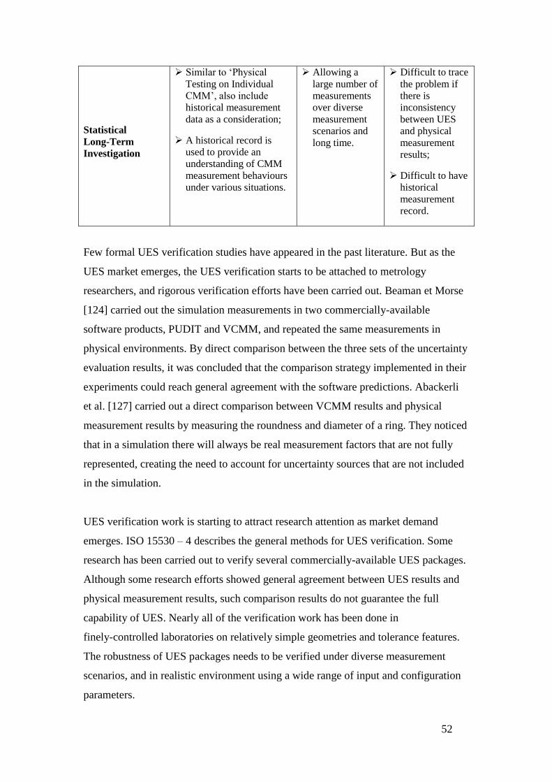
52

Statistical

Long-Term

Investigation

Similar to ‘Physical

Testing on Individual

CMM’, also include

historical measurement

data as a consideration;

A historical record is

used to provide an

understanding of CMM

measurement behaviours

under various situations.

Allowing a

large number of

measurements

over diverse

measurement

scenarios and

long time.

Difficult to trace

the problem if

there is

inconsistency

between UES

and physical

measurement

results;

Difficult to have

historical

measurement

record.

Few formal UES verification studies have appeared in the past literature. But as the

UES market emerges, the UES verification starts to be attached to metrology

researchers, and rigorous verification efforts have been carried out. Beaman et Morse

[124] carried out the simulation measurements in two commercially-available

software products, PUDIT and VCMM, and repeated the same measurements in

physical environments. By direct comparison between the three sets of the uncertainty

evaluation results, it was concluded that the comparison strategy implemented in their

experiments could reach general agreement with the software predictions. Abackerli

et al. [127] carried out a direct comparison between VCMM results and physical

measurement results by measuring the roundness and diameter of a ring. They noticed

that in a simulation there will always be real measurement factors that are not fully

represented, creating the need to account for uncertainty sources that are not included

in the simulation.

UES verification work is starting to attract research attention as market demand

emerges. ISO 15530 – 4 describes the general methods for UES verification. Some

research has been carried out to verify several commercially-available UES packages.

Although some research efforts showed general agreement between UES results and

physical measurement results, such comparison results do not guarantee the full

capability of UES. Nearly all of the verification work has been done in

finely-controlled laboratories on relatively simple geometries and tolerance features.

The robustness of UES packages needs to be verified under diverse measurement

scenarios, and in realistic environment using a wide range of input and configuration

parameters.

53

2.4 Chapter summary

In this chapter, the fundamentals of coordinate measurement, CMM measurement

planning and uncertainty evaluation simulation have been reviewed. The concepts of

coordinate measurement have been standardized in the international standard system.

There are many systems for computer-aided CMM measurement planning having

been developed to solve one or more CMM measurement challenges. These

developments have created a good foundation for the development of Uncertainty

Evaluation Software (UES), the software packages for evaluating task-specific

measurement uncertainty for CMM inspection. However, the performance of UES is

not universally agreed, hindering the industrial adoption of UES. One of the primary

reasons is that evaluating the task-specific measurement uncertainty, the key aim of

the UES, is a complex and sequential decision-making process, and there is a large

diversity and complexity of CMM resources and tasks. Determining the measurement

uncertainty as per ISO-VIM and ISO-GUM is complicated and abstract, and there is

some inconsistency between the ISO GPS standards. It is virtually impossible to

develop a CMM inspection planning algorithm which considers all of the problems

and parameters in the measurement process. Verifying the UES performance in a

physical environment has not been carried out comprehensively, and it is very

difficult to verify the UES results under all of the measurement scenarios.

Therefore, it is necessary to extend the UES verification studies into more

complicated and practical measurement scenarios. Moreover, it would be useful to

explore alternative approaches of utilizing UES evaluation results, and hence to

extend the applications of UES to a robust level. This is the major objective of the

thesis.

54

Chapter 3 Research Aims, Objectives and Methodology

This chapter presents the aims and specific objectives of the research. The general

research methodology in engineering has been discussed, and applied to this research

project.

3.1 Aim of the Research

On the basis of the literature review of the previous chapter, the aims of the research

are to verify the uncertainty simulation results of a particular UES software system

and to investigate the alternative means of utilizing the UES results. The physical

CMM measurement tasks will be carried out on a realistic-scale part under shopfloor

conditions. The physical measurement results will be compared with simulation

results in order to verify the UES performance and to identify alternative applications

of UES results. A new approach will be developed to provide an alternative means to

analysing UES results. The approach will analyse the UES results by embracing

statistical data analysing techniques. The statistics methods and characterizations will

be aligned into the CMM measurement. Hence, an approach suggesting a novel

perspective on UES application for CMMs will be established and proved.

The other broad aim of the research is to evaluate the newly developed Quality

Information Framework (QIF) from the perspective of using its constructs within

CMM measurement and inspection modelling and planning.

3.2 Objectives of the Research

To meet the aim of the research the following specific objectives have been

investigated:

1) To gain expert understanding on coordinate measurement, CMM measurement

modelling and uncertainty evaluation by literature review and industrial visits;

2) To verify UES performance under meaningful complexity measurement scenarios.

This objective will include:

55

a) Planning and carrying out the physical measurement on a real part under

shopfloor working conditions;

b) Simulating the same measurements using a UES system, and generating

simulation results;

c) Comparing physical and simulation measurement results;

3) To develop a novel measurement planning and implementation framework to

analyse and integrate digital and physical measurement uncertainty. The tasks

involved are:

a) To explore alternative applications of the UES by analysing the simulation

and physical measurement results;

b) Selecting statistical analysis method(s) which can be used for the

post-measurement data processing;

c) Aligning the statistical data analysing methods to the CMM measurement

reality;

4) To design and carry out test to validate the approach via the physical

measurements, define the details of the validation program, and draw conclusions;

5) To summarize the outcomes of the research, write papers and indentify future

research.

3.3 Methodology of the Research

3.3.1 Research methods in engineering

Generally, a research process follows either a deductive or inductive approach [128].

The inductive approach gathers data and then concludes a theory. The inductive

approach is more applicable to social science research. The deductive approach firstly

finds a theory (or a proposal) and is then tested with data. This is more appropriate to

engineering and science research, and is also adopted by this research.

56

According to the University of Bath, Mechanical Engineering course in Research

methods – ME50173 (2006), engineering research is described to have following

steps:

Encounter a problem;

Propose a solution;

Assess the consequences;

Decide How to embody the solution;

Embody it;

Test it;

Learn how dependable it was.

Blockley & Henderson [129] extended the above description, and further specified the

actions taken for engineering research:

Determine the basic area of the work;

Find out what is already known (review of previous work);

Identify the problem or gap exactly (problem definition and hypothesis

generation);

Develop a precise objective;

Perhaps propose and build a trial artefact;

Collect data on its performance;

Analyse the data;

Draw conclusions;

Disseminate findings.

3.3.2 Methods for this research project

The research methodology described above deals with an applied manufacturing

problem. It falls into our engineering research aim and objectives, and thus is adopted

by this research. Figure 18 lists the general research methodology in engineering

(highlighted in blue). The steps carried out in this research are underpinned by the

framework of general research and highlighted in red in Figure 18.

57

General research methodology in

engineering

Research methodology for this research

Fix the basic area of the work

Literature review to identify the problem and define the

aim and objectives – Chapter 2 & 3

Verify the UES performance under complicated

measurement scenarios – Chapter 4

Propose a framework to analyse UES results using

statistics approach – Chapter 5

Validate the framework and case study – Chapter 6

Conclusion and future work – Chapter 7

Develop a precise objective

Identify the problem or gap

Find out what is already known

Propose and build a trial artefact

Collect data on its performance

Analyse the data

Draw conclusions

Disseminate findings

Background, scope and contents of the thesis –

Chapter 1

(1)

(2)

(3)

(4)

(5)

(6)

Figure 18. Research method of this project

(1) Determine the basic area of the work - Background

In Chapter 1 – Background, scope and justification, the basic research area of the

work has been briefly introduced. The research area has been determined in the

verification of CMM measurement simulation for the complex product inspection and

assembly.

(2) Research problem definition and hypotheses - Literature review

As shown in Chapter 2, the literature review conducted in this research included a

current review from the academic and industrial points of view. Literature on the

fundamentals of coordinate measurements, computer-aided CMM measurement

planning and the development of uncertainty simulation techniques were thoroughly

surveyed and those relevant to the research reviewed. The literature review has been

used extensively to aid the understanding of current research activities of the UES

verification and application, to avoid repeating research, developing aims and

objectives to aid the construction of the hypotheses.

58

Following Chapter 2, the gaps in CMM measurement planning and modelling were

identified and hypotheses generated in this chapter (Chapter 3). The hypotheses can

be summarised as:

Metrology will play a vital role in the modern manufacturing, interlinking all of

the phases within a product lifecycle, from design, manufacturing, in-service to

maintenance;

Task-specific measurement uncertainty will play a leading role in measurement

uncertainty evaluation;

The performance of task-specific measurement uncertainty evaluation software

(UES) is not promising. There is a need to verify the UES performance

particularly under complicated measurement scenarios;

The UES results can be used to guide practical industrial production if being

deployed with more dedicated data analysis approach, e.g. Design of Experiments

(DOE);

The Design of Experiments (DOE) framework in the research serves for the

post-measurement data processing. It does not deal with the CMM inspection

process improvement and conformance assessment.

(3) Developing precise objectives – Pilot experiment

The aims and objectives of the research have been described in Section 3.1 and 3.2.

The more precise objectives have been developed in Chapter 4, where a pilot study of

UES verification has been carried out in the shopfloor environment, and hence the

limitation of UES capability has been realized.

(4) Proposing and building a prototype system – Proposing a DOE framework

To achieve the aims and objectives and realize the hypotheses, a novel framework

which is deployed by the Design of Experiments (DOE) approach is firstly proposed

and then implemented.

The proposed framework has three main modules: measurement scenario streamliner

module, measurement uncertainty simulation module and post-measurement data

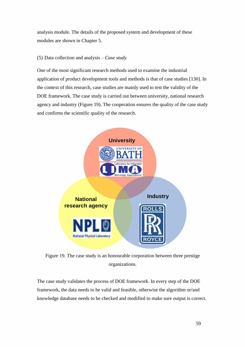
59

analysis module. The details of the proposed system and development of these

modules are shown in Chapter 5.

(5) Data collection and analysis – Case study

One of the most significant research methods used to examine the industrial

application of product development tools and methods is that of case studies [130]. In

the context of this research, case studies are mainly used to test the validity of the

DOE framework. The case study is carried out between university, national research

agency and industry (Figure 19). The cooperation ensures the quality of the case study

and confirms the scientific quality of the research.

University

National

research agency

Industry

Figure 19. The case study is an honourable corporation between three prestige

organizations.

The case study validates the process of DOE framework. In every step of the DOE

framework, the data needs to be valid and feasible, otherwise the algorithm or/and

knowledge database needs to be checked and modified to make sure output is correct.

60

Also by using the case studies, the performance of the DOE framework can be

identified.

Data collection and analysis has been carried out through the case study. The DOE

framework developed in the research is required to quantitatively evaluate the

influences of the uncertainty contributors of the CMM measurement. The main

concept of the case study is to validate the DOE results by the physical measurements.

The simulation data sets are collected through the commercial UES package,

PUNDIT/CMM, and analysed in the statistics software Minitab. In parallel, the

physical measurement data sets are collected in a finely-controlled environment. At

last, the two data sets are compared using NIST statistical comparison methods to find

out the statistical significance. The details of the case study are presented in Chapter

6.

(6) Conclusion and dissemination of findings – Conclusion and future work

The findings are disseminated as a thesis, and as publications in conferences and

journals. The conclusion and the future work of the research are presented in Chapter

7.

61

Chapter 4 Initial Study of Establishing Task Specific

Uncertainty using a Digital CMM Model and Physical

Measurements

4.1 Introduction to the Digital CMM Model

The digital CMM Model is usually a software package developed for evaluating the

task-specific CMM measurement uncertainty. A commercial software system,

PUNDIT, is employed in the research to demonstrate the performance of digital CMM

model. Based on the uncertainty predicted by the CMM model, further research is

developed. This section introduces the working principles and the operations flow of

the simulation software, and provides a demonstration study of using the CMM

modelling software.

The digital CMM system, PUNDIT, can be considered as a UES according to the

description of the standards. However, as PUNDIT does much more than uncertainty

estimation, it is only appropriate to describe it as digital CMM modelling system.

4.1.1 Working principle

The CMM measurement modelling software evaluates the task-specific measurement

uncertainty by the Simulation-by-Constrain (SBC) method, an uncertainty simulation

method reviewed in Chapter 2 – Literature Review. It performs the Monte Carlo

simulations regarding principal sources of error in CMM measurements by taking into

account machine geometry, probe, thermal conditions, feature surface characteristics,

sampling patterns, etc, as shown in Figure 20. It has a modular architecture that

facilitates enhancements of error models [22]. Deviation errors with random values are

added to the actual figures on each parameter. The combined uncertainty is obtained by

having the integration of the individual random errors into one uncertainty value [21].

62

CMM Geometry

WorkpieceFactors

Environment

SensorSystem

Data Analysis

SamplingStrategy

Figure 20 Error sources considered in CMM modelling software

As its first step in creating the uncertainty estimates, the CMM modelling software

incorporates a ‘Bounding Measurement Set’, which is a hypothetical CMM error states

found to be consistent with the ASME B89 test suite [123]. Since this set does not

completely describe the CMM, the software then proceeds to simulate inspection of the

part using each of the hypothetical CMMs in this set by randomly varying the errors of

each error contributor within the ‘Bounding Measurement Set’. Finally, for each

GD&T parameter to be determined the population of substitute geometry errors is used

to create an estimate of measurement uncertainty [131]. The inspection engineers can

use this estimation of measurement uncertainty as the guidance for setting up the

practical CMM probing strategy and companies can avoid the need to physically error

map all of the CMMs, which is an expensive and impractical activity for industry.

4.1.2 Operations flow

The operations flow of the CMM modelling software is fairly straight forward and

similar to the CMM measurement planning in a physical environment. Figure 21

shows the entire operations flows [131]. It starts from loading the workpiece CAD

model to the system. Then the users can manually characterize the factors appearing

during the CMM measurement process. These factors include the CMM, probe,

environment (mainly thermal environment), measurement plan and manufacturing

63

information. At last, the software runs Monte-Carlo Simulation and calculates the

measurement results.

Workpiece CMM Probe

EnvironmentMeasurement planManufacturing info

Results

Figure 21 Operations flow (concluded from [131]).

Monte Carlo Simulation is a broad class of computational algorithms that rely on

repeated random sampling to obtain numerical results [27]. As shown in Figure 22,

)(xf represents a measurement process. )( 1xg , )( 2xg and )( 3xg

are the

distribution functions of the input quantities, which represent the influence quantities

of the measurement process. Through the function box )(xf , )(yg is propagated to

represent the distribution function of the measurement results.

64

Figure 22 Monte Carlo simulation applied to metrology

To realize the operations flow of the digital CMM model, a brief study was organised

for measuring a mechanical product with complex geometry.

Figure 23 CAD model of the complex product for the case study.

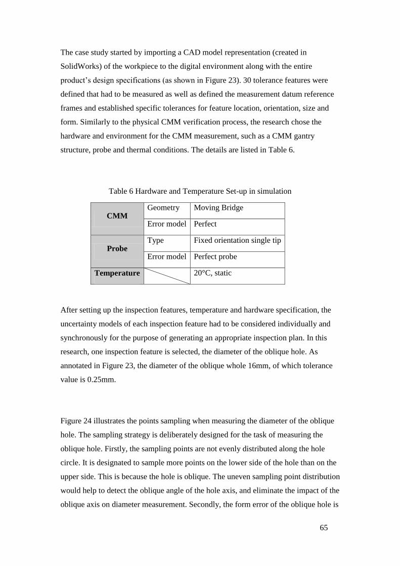
65

The case study started by importing a CAD model representation (created in

SolidWorks) of the workpiece to the digital environment along with the entire

product’s design specifications (as shown in Figure 23). 30 tolerance features were

defined that had to be measured as well as defined the measurement datum reference

frames and established specific tolerances for feature location, orientation, size and

form. Similarly to the physical CMM verification process, the research chose the

hardware and environment for the CMM measurement, such as a CMM gantry

structure, probe and thermal conditions. The details are listed in Table 6.

Table 6 Hardware and Temperature Set-up in simulation

CMM Geometry Moving Bridge

Error model Perfect

Probe Type Fixed orientation single tip

Error model Perfect probe

Temperature 20°C, static

After setting up the inspection features, temperature and hardware specification, the

uncertainty models of each inspection feature had to be considered individually and

synchronously for the purpose of generating an appropriate inspection plan. In this

research, one inspection feature is selected, the diameter of the oblique hole. As

annotated in Figure 23, the diameter of the oblique whole 16mm, of which tolerance

value is 0.25mm.

Figure 24 illustrates the points sampling when measuring the diameter of the oblique

hole. The sampling strategy is deliberately designed for the task of measuring the

oblique hole. Firstly, the sampling points are not evenly distributed along the hole

circle. It is designated to sample more points on the lower side of the hole than on the

upper side. This is because the hole is oblique. The uneven sampling point distribution

would help to detect the oblique angle of the hole axis, and eliminate the impact of the

oblique axis on diameter measurement. Secondly, the form error of the oblique hole is

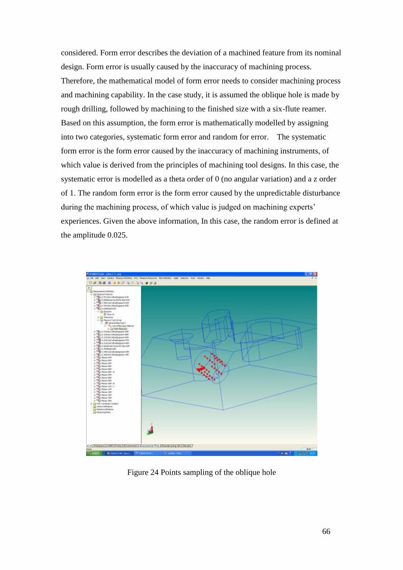
66

considered. Form error describes the deviation of a machined feature from its nominal

design. Form error is usually caused by the inaccuracy of machining process.

Therefore, the mathematical model of form error needs to consider machining process

and machining capability. In the case study, it is assumed the oblique hole is made by

rough drilling, followed by machining to the finished size with a six-flute reamer.

Based on this assumption, the form error is mathematically modelled by assigning

into two categories, systematic form error and random for error. The systematic

form error is the form error caused by the inaccuracy of machining instruments, of

which value is derived from the principles of machining tool designs. In this case, the

systematic error is modelled as a theta order of 0 (no angular variation) and a z order

of 1. The random form error is the form error caused by the unpredictable disturbance

during the machining process, of which value is judged on machining experts’

experiences. Given the above information, In this case, the random error is defined at

the amplitude 0.025.

Figure 24 Points sampling of the oblique hole

67

When all the influencing parameters have been specified, the number of 1,000

simulation cycles was selected to run and launch the simulation process.

4.1.3 The outputs

The Monte-Carlo simulation runs in the CMM measurement modelling software, and

outputs task-specific uncertainty estimates for the dimensions measured.

Figure 25 is the outputs of the simulation study in previous section. This simulation

results state the bias, variability and uncertainty estimation of task-specific

measurement. Ideally, the shape of the results is close to a normal distribution due to the

Monte Carlo simulation used. For the inspected oblique hole, the task-specific

measurement uncertainty statement can be expressed as “The uncertainty of the

diameter of this nominally 16 mm diameter hole is 0.121 mm, at 95% confidence.”

Figure 25 Simulation Result

68

4.2 Pilot case study on verifying Digital CMM Model simulation

results by physical measurements on a large scale component

4.2.1 Background

As stated in previous sections, estimation of the CMM measurement uncertainty for

real parts is a sophisticated undertaking. The ability of the uncertainty estimation

software remains arguable in terms of their accuracy and precision. In order to test the

performance of the uncertainty estimation software (UES) used, the physical and

virtual measurements have been carried out on a large-scale part, on which the critical

and relatively small-size features needed to inspected by CMM to meet their tight

tolerance requirements. The part is an essential component on a high-quality

aerospace product. The main challenge of the component is the fitting/assembly

problem. The physical measurement was carried out in an industrial aerospace facility

in the UK.

Prior to carrying out the physical measurements on the component, it is advised to

firstly identify the likely sources that would affect the measurement uncertainty. The

sources affecting the measurement uncertainty are identified as:

Variation in ambient temperature;

Variation in component temperature;

Choice of probing stylus;

Condition of the stylus (degree of wearing, damage or cleanliness);

Location of the component on CMM measurement volume;

Variation in the location of the part in any fixture used on the CMM table;

Machine to machine variation if two or more CMM are used in parallel on

the same part;

Variation between part programmes if more than one programme version is

used to control the inspection procedure on the same part;

Operator influence through variation in set up, probe qualification, datuming

practice or assessment of probe qualification results.

69

The above sources affecting measurement uncertainty are prioritized and grouped.

According to the aims and objectives of this research and research facility availability,

the following sources affecting measurement uncertainty are included in the study:

CMM;

Probe;

Temperature;

Measurement plan.

Although there are other uncertainty contributors, it is proposed that for the pilot

study, these other uncertainties are assumed to be small, and, hence can be ignored.

Additionally the following assumptions have been made:

Form errors are not a significant contributor to measurement uncertainty in

this case, and consequently can be ignore;

The error in machine location at any given point is not a function of how the

CMM got to that point. In other words, the dynamic errors are not considered

to be significant;

The part is perfectly constrained and not deformed by its fixture.

These assumptions are established given the metrology experts’ experiences and the

aims and the objectives of the research. The assumptions have made the pilot study

practicable in the shopfloor environment, and linked the study outcomes to the

research aims. Not only have the assumptions been made on reasonable ground, but

also they have provided an industrial focus to the case study.

4.2.2 Physical measurements on a large-scale part with relatively small-size

feature

Due to the data protection agreement with the industrial partner, the specific

information relating to the inspected part design and manufacturing are advised to be

non-disclosure. Generally speaking, the inspected part is a key component of a gas

turbine system which generates enormous and reliable power to drive high-tech

engineering products. The inspected part is the stator of the gas turbine system. As

circled in the red loop in Figure 26, it is located behind the rotary compressor to

uniform the gas flow exiting the compressor.

70

Figure 26 A representation of the gas turbine system

Figure 27 is a highly simplified representation of the inspected part. It is a large scale

part, of which the diameter is approximately 3 meters. Various holes are drilled on the

inspected part in order to rivet the inspected part with the housing hole. The positions

of the holes and the geometries of the inspected part are constrained with tight

tolerances. A very large coordinate measurement machine (CMM) is used to carry out

measurement tasks. However, it is challenging to determine a confident measurement

statement because of the unexceptionally large scales of the part and the CMM.

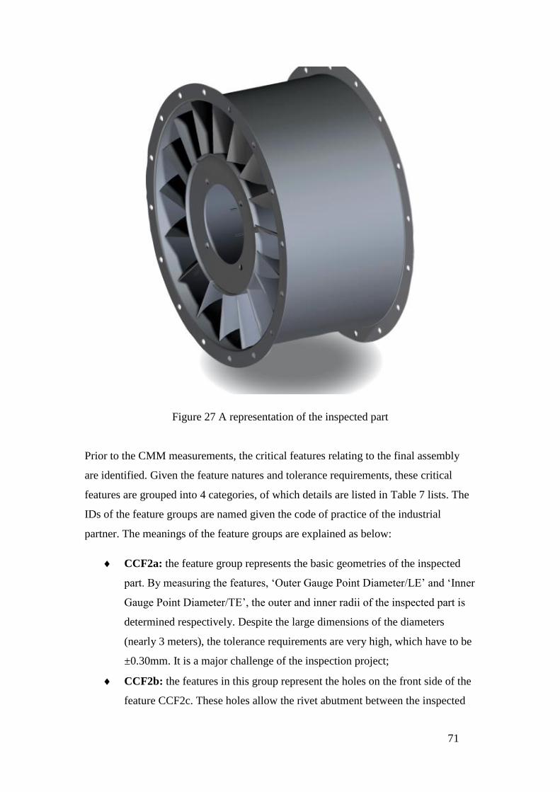
71

Figure 27 A representation of the inspected part

Prior to the CMM measurements, the critical features relating to the final assembly

are identified. Given the feature natures and tolerance requirements, these critical

features are grouped into 4 categories, of which details are listed in Table 7 lists. The

IDs of the feature groups are named given the code of practice of the industrial

partner. The meanings of the feature groups are explained as below:

CCF2a: the feature group represents the basic geometries of the inspected

part. By measuring the features, ‘Outer Gauge Point Diameter/LE’ and ‘Inner

Gauge Point Diameter/TE’, the outer and inner radii of the inspected part is

determined respectively. Despite the large dimensions of the diameters

(nearly 3 meters), the tolerance requirements are very high, which have to be

±0.30mm. It is a major challenge of the inspection project;

CCF2b: the features in this group represent the holes on the front side of the

feature CCF2c. These holes allow the rivet abutment between the inspected

72

part and the housing shell. By measuring these holes, the positions of these

holes are constrained to allow smooth joint between the inspected part and

the housing shell;

CCF2d: the features in this group represent the holes on the rear side of the

feature CCF2c. These holes have the same function as the ones in the feature

group CCF2b. By measuring these holes, the positions of these holes are

constrained to allow smooth joint between the inspected part and the housing

shell.

Table 7 The list of the inspected features

ID Feature Description Nominal

(mm)

Tolerance

(mm)

CCF2a Outer Gauge Point Diameter/LE

2981.8 ±0.30

Inner Gauge Point Diameter/TE§ 2946.78 ±0.30

CCF2b

Front Flange Bolt Hole Position/No1 791 ±0.25

Front Flange Bolt Hole Position/No15 791 ±0.25

Front Flange Bolt Hole Position/No45 791 ±0.25

CCF2d

Rear Flange Bolt Hole Position/No1 805 ±0.25

Rear Flange Bolt Hole Position/No7 805 ±0.25

Rear Flange Bolt Hole Position/No14 805 ±0.25

Rear Flange Bolt Hole Position/No20 805 ±0.25

Note: LE: Leading Edge;

§TE: Tailing Edge (sic).

The specifications of the CMM used in the test is listed in Table 8. The CMM is a

bridge type CMM with exceptionally large working volume ( mmm 444 ). The

CMM gantry is firmly embedded into the ground of shop floor. The maximum

permitted error (MPE) of the CMM is mmmmLmm 1000/)(109 quoted by

the manufacturer’s manual. The probe is the Renishaw SP25M. According the

temperature monitor in the shopfloor, the temperature control is CC 05.052.19 . The

inspected part is clamped on the ground by special fixtures within the CMM working

volume. Considering the large scale of the inspected part, the form errors are assumed

to be ignored.

73

Table 8 The physical test parameters of the CMM

Working Volume (approximate) mmm 444

MPE Quoted by Manufacturer mmmmLmm 1000/)(109

Probe Renishaw SP25M

Temperature CC 05.052.19

Manufacturing Assume no form error

The measurement plan is established as follows:

1) Calibration: Measure 4 points on a calibrated sample of holes to get the

self-calibration;

2) Datum establishment: Probing 3 points on top face of the inspected part to create a

plane. Then, probing 4 points on one of the Front Flange Bolt Holes to create a

circle;

3) Feature Group CCF2a Measurement: Probing certain critical points by following

the commands of the metrology experts in the shopfloor. The diameters of the

inner circle and the outer circle of the inspected part are calculated and reported

using the least-square fitting algorithm;

4) Feature Groups CCF2b and CCF2d Measurement: the holes are measured by

probing 4 points at the 2mm depth of the hole. The position of the holes are

calculated, and fitted using least square fitting algorithm.

All of the features listed in Table 7 have been measured by the CMM machine within

8 hours. The measurement results are listed in Table 9. The measurement results of

Feature Groups CCF2b and CCF2d, which indicate the hole positions, were originally

reported in polar coordinates. The results listed in Table 9 have been converted to

Cartesian coordinates in order to calculate the positional deviation.

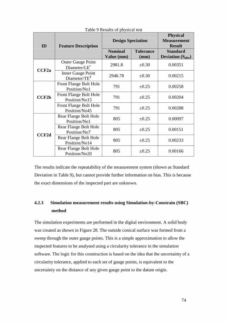
74

Table 9 Results of physical test

ID Feature Description

Design Speciation

Physical

Measurement

Result

Nominal

Value (mm)

Tolerance

(mm)

Standard

Deviation (Sphy)

CCF2a

Outer Gauge Point

Diameter/LE

2981.8 ±0.30 0.00351

Inner Gauge Point

Diameter/TE§

2946.78 ±0.30 0.00215

CCF2b

Front Flange Bolt Hole

Position/No1 791 ±0.25 0.00258

Front Flange Bolt Hole

Position/No15 791 ±0.25 0.00204

Front Flange Bolt Hole

Position/No45 791 ±0.25 0.00288

CCF2d

Rear Flange Bolt Hole

Position/No1 805 ±0.25 0.00097

Rear Flange Bolt Hole

Position/No7 805 ±0.25 0.00151

Rear Flange Bolt Hole

Position/No14 805 ±0.25 0.00233

Rear Flange Bolt Hole

Position/No20 805 ±0.25 0.00166

The results indicate the repeatability of the measurement system (shown as Standard

Deviation in Table 9), but cannot provide further information on bias. This is because

the exact dimensions of the inspected part are unknown.

4.2.3 Simulation measurement results using Simulation-by-Constrain (SBC)

method

The simulation experiments are performed in the digital environment. A solid body

was created as shown in Figure 28. The outside conical surface was formed from a

sweep through the outer gauge points. This is a simple approximation to allow the

inspected features to be analysed using a circularity tolerance in the simulation

software. The logic for this construction is based on the idea that the uncertainty of a

circularity tolerance, applied to each set of gauge points, is equivalent to the

uncertainty on the distance of any given gauge point to the datum origin.

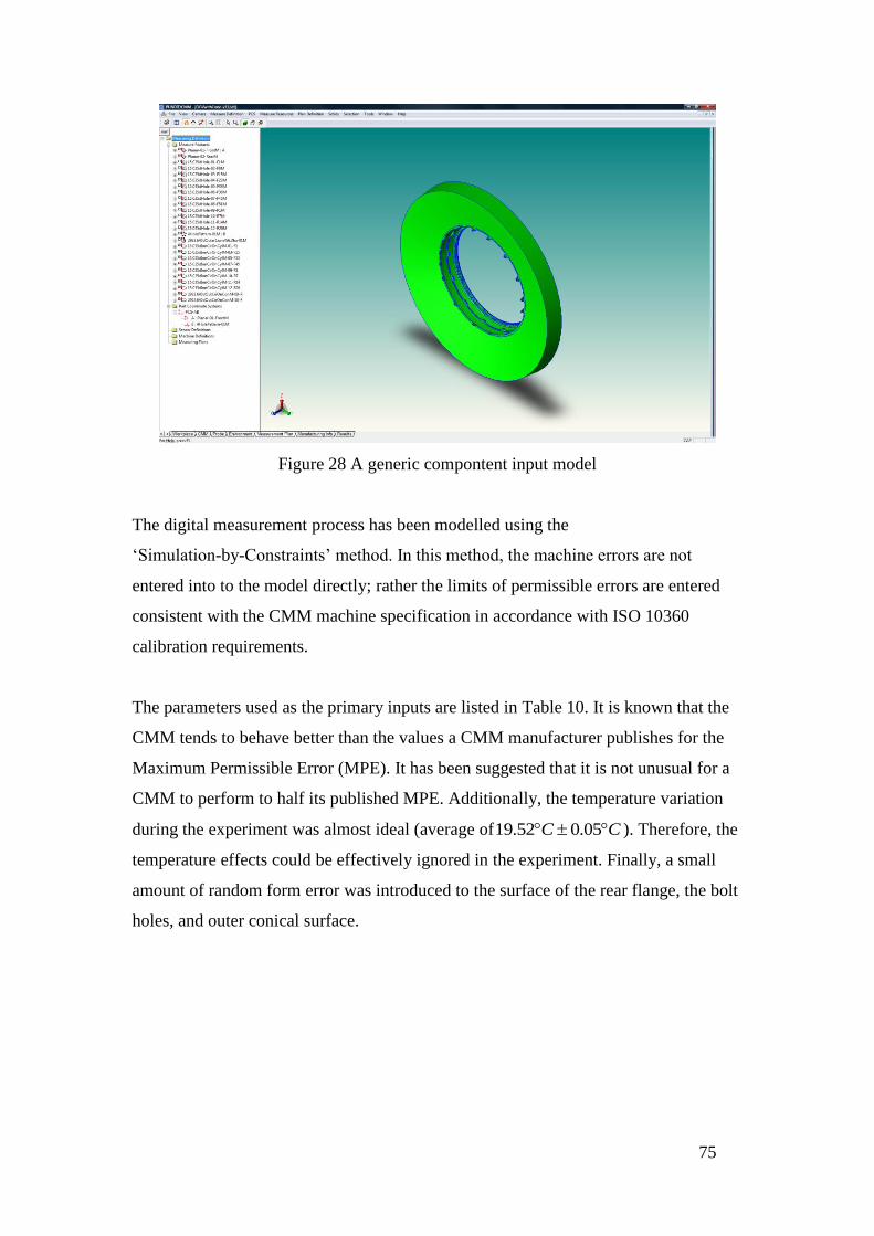
75

Figure 28 A generic compontent input model

The digital measurement process has been modelled using the

‘Simulation-by-Constraints’ method. In this method, the machine errors are not

entered into to the model directly; rather the limits of permissible errors are entered

consistent with the CMM machine specification in accordance with ISO 10360

calibration requirements.

The parameters used as the primary inputs are listed in Table 10. It is known that the

CMM tends to behave better than the values a CMM manufacturer publishes for the

Maximum Permissible Error (MPE). It has been suggested that it is not unusual for a

CMM to perform to half its published MPE. Additionally, the temperature variation

during the experiment was almost ideal (average of CC 05.052.19 ). Therefore, the

temperature effects could be effectively ignored in the experiment. Finally, a small

amount of random form error was introduced to the surface of the rear flange, the bolt

holes, and outer conical surface.

76

Table 10 Simulation parameters

CMM E = ±4.5μm + 5μm * [L (mm)/1000 mm]

(half the manufacturers’ stated MPE)

Probe Standard Deviation 1.0μm for 100m stylus

Environment CC 020 (minor change – to remove temperature effects

from the simulation)

Manufacturing 5µm random error on rear flange, holes and conical surface

Each simulation trial was conducted with 3,000 runs. The simulation results are listed

in Table 11.

Table 11 Simulation result

ID Feature

Simulation Result

Standard Deviation

(Spun)

Uncertainty

(Upun)

CCF2a Gauge Points (LE) 0.004377 0.0173

Gauge Points (TE) 0.004300 0.0171

CCF2b

Front Hole 1 (Pos) 0.005707 0.0210

Front Hole 15 (Pos) 0.006611 0.0262

Front Hole 45 (Pos) 0.006639 0.0265

CCF2d

Rear Hole 1 (Pos) 0.005335 0.0197

Rear Hole 7 (Pos) 0.006346 0.0249

Rear Hole 14 (Pos) 0.005245 0.0196

Rear Hole 20 (Pos) 0.006842 0.0275

4.2.4 Measurement results comparison

A) Comparison between physical and digital measurement results

The physical measurement results and the digital measurement results are listed

together in Table 12. Spun is the standard deviation predicted by the digital CMM

model, and Sphy is the standard deviation of the physical tests. Spun/Sphy is the ratio of

standard deviation by simulation versus the standard deviation from the physical

repeatability test.

77

Table 12 Comparison between digital and physical measurement results

ID Feature Tolerance

(mm)

Physical

Measurement Digital Measurement

Ratio

Spun/Sphy Standard

Deviation

(Sphy, mm)

Mean

Error

(mm)

Standard

Deviation

(Sphy, mm)

CCF2a

Gauge

Points

(LE)

0.30 0.00351 0.008575 0.004377 1.25

Gauge

Points

(TE)

0.30 0.00215 0.008453 0.0043 2.00

CCF2b

Front

Hole 1

(Pos)

0.25 0.00258 0.009567 0.005707 2.21

Front

Hole 15

(Pos)

0.25 0.00204 0.012934 0.006611 3.24

Front

Hole 45

(Pos)

0.25 0.00288 0.013244 0.006639 2.31

CCF2d

Rear

Hole 1

(Pos)

0.25 0.00097 0.00901 0.005335 5.50

Rear

Hole 7

(Pos)

0.25 0.00151 0.012233 0.006346 4.20

Rear

Hole 14

(Pos)

0.25 0.00233 0.00907 0.005245 2.25

Rear

Hole 20

(Pos)

0.25 0.00166 0.013847 0.006842 4.12

Given the data in Table 12, Figure 29 is constructed.

78

0

0.001

0.002

0.003

0.004

0.005

0.006

0.007

0.008

Gauge

Points

(LE)

Gauge

Points

(TE)

Front

Hole 1

(Pos)

Front

Hole

15

(Pos)

Front

Hole

45

(Pos)

Rear

Hole 1

(Pos)

Rear

Hole 7

(Pos)

Rear

Hole

14

(Pos)

Rear

Hole

20

(Pos)

Std

Dev

(n

m)

0

1

2

3

4

5

6

Ratio

Physical Measurement

Simulation Results

Ratio Between Simulation and Physical Measurement Results

Figure 29 Comparison between physical measurement and simulation results

From Figure 29, several points can be concluded:

The digital CMM model generally predicts higher measurement results than that

obtained from the physical measurement environment. The standard deviations for

positional measurements obtained from the digital measurement environment are

generally higher than that obtained through physical experiments.

This is caused by the nature of the SBC method. The SBC method does not

require a full description of the physical measurement environment. The

information loaded into the digital CMM model (which employs SBC method)

does not completely cover all aspects of measurement process. Therefore, the

measurement uncertainty predicted by the digital CMM model would be

generally higher than that obtained from the physical measurement.

The Ratio between Simulation and Physical Measurement Results varies

significantly across the inspected features. The Ratio ranges from 1.25 to 5.50.

For the Feature Group CCF2a, which includes ‘Gauge Points (LE)’ and ‘Gauge

Points (TE)’, the Ratio is relatively lower, ranging between 1.25 to 2.00. In

79

particular, for the ‘Gauge Point (LE), the standard deviations predicted by

simulation software become closer to physical measurement results. The Feature

Group CCF2a represents the outer and inner diameters of the inspected part. The

CCF2a measurements represent the measurements of size and dimension. The

comparison result shows promising capability of the digital CMM model in

predicting the dimension measurements.

For the Feature Group CCF2b, which includes three holes at the flange bolt fronts,

the Ratio gets larger, and the variations are larger. It indicates that the

performance of the digital CMM model is unstable in predicting the locations of

these front holes.

For the Feature Group of CCF2d, which includes four holes at the flange bolt

rears, the Ratio get significantly larger and variation increase. Despite

disregarding the human errors during the physical measurement process, the Ratio

values and its variation are not considered to be acceptable. In particular, there are

significant differences in measurement results on Rear Hole 1.

The above examinations on the Ratio between Simulation and Physical

Measurement Results indicate the unstable performance of the digital CMM

model in predicting different feature. Generally, the digital CMM model is more

capable of ‘measuring’ the dimension features (diameter in the pilot study) than

the form features (hole positions in the pilot study). This conclusion is close to

common understandings on uncertainty estimation software. Form features have

high geometric complexity. Estimating measurement uncertainty for form

measurement needs more comprehensive and sophisticated algorithms than that

for dimension measurement. Consequently, in the pilot study, the digital CMM

model performs better to predict the diameter measurement than the hole

positions.

The human-errors are considered. At the Rear Hole 1 (Pos), the ratio is

significantly high. It is very difficult to give a definitive explanation. It is very

possible that the significant high ratio value was caused by un-detected human

errors over the physical measurement process.

80

Generally speaking, no obvious tendency can be derived by simply comparing

physical measurements and simulation results. The performance of the digital CMM

model is not convincing. The digital measurement results are not reasonably close to

the physical measurement results. The large dimension and complex geometry of the

inspected part is a major problem. Through the measurement modeling process of the

pilot study, it is realized that the digital CMM model would be more suitable to

measure conventionally machining products, of which dimensions are within

traditional CMM working volume.

B) Calculating measurement uncertainty using GUM approach

Another approach to justifying the measurement results has been carried out by using

the GUM approach, the standardized guidance for measurement uncertainty

calculation. The GUM-approach measurement uncertainty is calculated given the

mathematically idealized conditions of measurement instruments and measurement

environments. The CMMs and measurement environments which vary in the ideal

mathematical ways are nicknamed as ‘being good’ in the shopfloor. Therefore, the

GUM-approach measurement uncertainty represents the measurement uncertainty of a

‘good’ CMM in a ‘good’ measurement environment. The comparisons between the

GUM-approach measurement uncertainty and digital measurement uncertainty

examine the consistence between the digital CMM model and the GUM method.

Priory to the comparisons, the measurement uncertainties are calculated using the

GUM approach.

The GUM advises that a value for uncertainty can be calculated by identifying the

uncertainty component sources and adding these values in quadrature [21]. Generally,

it is considered a CMM measurement system as having three major categories of

uncertainty: the CMM machine itself, the temperature effects, and random error

(‘Type A’). In our case, the temperature, as monitored as CC 05.052.19 , is likely to

be a small contributor to the overall uncertainty, and therefore is ignored. Therefore,

the uncertainty is approximated using the GUM method by considering just the MPE

of CMM machine and the Type A contribution (as calculated from the standard

deviation of the repeatability test).

81

In order to calculate the GUM-approach uncertainty (UGum), a combined standard

uncertainty was calculated by adding constituent standard uncertainties in quadrature,

and multiplying by a coverage factor of 2. This gives a value of expanded uncertainty

of 95%. The CMM uncertainty used for calculation was taken by the value for the

anticipated error from the MPE value at the nominal length and dividing by 3 (as

the distribution is assumed to be rectangular). The Type A uncertainty is calculated by

taking the standard deviation and dividing by 10 , where 10 is the number of values

used in the test.

The measurement uncertainties calculated given the GUM approach are listed in Table

13 together with the digital measurement uncertainty. The ratio between

GUM-approach uncertainty and digital measurement uncertainty is also calculated

and listed in Table 13.

82

Table 13 GUM-approach measurement uncertainty and digital measurement

uncertainty

Feature

Digital Measurement GUM-approach

Uncertainty Ratio

Upun/

UGUM

Standard

Deviation

(Spun)

Uncertainty

Upun CMM Type A UGUM

Gauge

Points (LE) 0.004377 0.0173 0.0069 0.0011 0.0140 1.2

Gauge

Points (TE) 0.0043 0.0171 0.0069 0.0007 0.0138 1.2

Front Hole

1 (Pos) 0.005707 0.0210 0.0049 0.0008 0.0099 2.1

Front Hole

15 (Pos) 0.006611 0.0262 0.0049 0.0006 0.0098 2.7

Front Hole

45 (Pos) 0.006639 0.0265 0.0049 0.0009 0.0099 2.7

Rear Hole 1

(Pos) 0.005335 0.0197 0.0049 0.0003 0.0099 2.0

Rear Hole 7

(Pos) 0.006346 0.0249 0.0049 0.0005 0.0099 2.5

Rear Hole

14 (Pos) 0.005245 0.0196 0.0049 0.0007 0.0100 2.0

Rear Hole

20 (Pos) 0.006842 0.0275 0.0049 0.0005 0.0099 2.8

Note: 1) In this table, uncertainty is calculated as the mean error plus two times of

standard deviation, U=E+2σ;

2) The GUM-approach measurement uncertainty, UGUM, is calculated in the

following way:

a) Calculate type A uncertainties given the equation

n

xn

xxn

U

n

i

n

i

iii

A

1 1

)1

(1

1

where the subscript A indicated the uncertainty type, and ix represents

the measurement results, and n represents the number of repeated

measurements.

b) Calculate type B uncertainties: two ‘systematic’ uncertainty sources are

included, which are CMM specification and temperature effects;

c) All type A and Type B uncertainties were combined in quadrature to

derived the combined standard uncertainty;

83

d) Calculate effective degrees of freedom to derive the appropriate K value

from a t-distribution table. In this calculation, K=2.

C) Comparison between digital measurement uncertainty and GUM-approach

measurement uncertainty

To compare the digital measurement uncertainty with the GUM-approach

measurement uncertainty, Figure 30 is drawn given the data in Table 13.

0.0000

0.0100

0.0200

0.0300

0.0400

0.0500

0.0600

Gauge

Points

(LE)

Gauge

Points

(TE)

Front

Hole 1

(Pos)

Front

Hole 15

(Pos)

Front

Hole 45

(Pos)

Rear Hole

1 (Pos)

Rear Hole

7 (Pos)

Rear Hole

14 (Pos)

Rear Hole

20 (Pos)

Un

cert

ain

ty (

nm

)

0.0

0.5

1.0

1.5

2.0

2.5

3.0

Rati

oGUM Uncertainty Simulation Uncertainty Ratio between Simulation/GUM Uncertainty

Figure 30 Uncertainty comparison between simulation result and GUM calculation

From Figure 30, it can be seen that the digital measurement uncertainty is

significantly higher than the GUM-approach measurement uncertainty. It again

reflects the nature of the SBC method, which the limited information input to the

digital CMM model restrains the fidelity of the digital measurement result.

On the other hand, the values of the Ratio between the digital measurement

uncertainty and the GUM-approach measurement uncertainty vary given the nature of

the inspected features. At the features of ‘Gauge Points (LE)’ and ‘Gauge Points (TE)’

(Feature Group CCF2a), which represent the dimension measurement, the Ratio

84

values get close to 1 and become stable. However, for the rest of the feature

measurements, which represent the geometry measurements, the Ratio values vary

significantly, and few tendencies could be examined. It further proves that it is very

complicated and difficult to simulate geometry measurement in the digital

environment. The digital CMM model needs to improve the capability of predicting

geometry measurement uncertainty.

For further analyzing the performance of the simulation results, the Simulation/GUM

Ratio* and the Simulation/Physical Ratio

† are compared, and their value variations

are illustrated in Figure 31. The values of Simulation/GUM Ratio vary between 1.2 to

2.8, whereas the values of Simulation/Physical Ratio vary between 1.25 to 4.20. The

Simulation/GUM ratio is generally lower than ‘Simulation/Physical ratio’, and the

Simulation/GUM Ratio is more convergent than ‘Simulation/Physical Ratio’. The

digital measurement uncertainty tends to be closer to the GUM-approach

measurement uncertainty to the physical measurement uncertainty. It indicates that the

digital CMM model has relatively good consistence with the GUM approach. The

uncertainty calculation algorithm utilized by the digital CMM model incorporates

well with the GUM instructions which are fundamental to measurement uncertainty

estimation. But the digital CMM model still needs to improve its performance in the

physical measurement environment.

*Simulation/GUM Ratio: the Ratio between the digital measurement uncertainty and the GUM-approach

measurement uncertainty; † Simulation/Physical Ratio: the Ratio between the digital measurement uncertainty and the physical measurement

uncertainty.

85

0.0

1.0

2.0

3.0

4.0

5.0

6.0

Gauge

Points (LE)

Gauge

Points (TE)

Front Hole

1 (Pos)

Front Hole

15 (Pos)

Front Hole

45 (Pos)

Rear Hole

1 (Pos)

Rear Hole

7 (Pos)

Rear Hole

14 (Pos)

Rear Hole

20 (Pos)

Ra

tio

Simulation/Physical Ratio Simulation/GUM Ratio

Figure 31 Comparison between simulation result, physical measurement result and

GUM approach result.

Noticeably, in Figure 31, the difference between the Simulation/Physical Ratio and

the Simulation/GUM Ratio at Rear Hole 1 (Pos) is significantly high. As explained in

previous paragraphs, the unexpectedly high Simulation/Physical Ratio is possibly

caused by human errors during the physical measurement process. Consequently, it

causes the unexpected high difference between the two ratios. However, it suggests

that the digital CMM model could be used to detect physical operation errors, which

alert production managers to examine the physical measurement process to prevent

the errors occurring again.

Conclusively, four major points can be made from the above comparisons:

1) The digital CMM model generally predicts higher measurement uncertainty than

GUM-approach uncertainty and physical measurement uncertainty. This indicates

the nature of the SBC methods;

2) The digital CMM model is more capable of predicting dimension measurement

uncertainty than geometry measurement uncertainty. Estimating uncertainty for

geometry measurement is sophisticated and difficult;

3) The digital CMM model has relatively good consistency with the GUM

instructions, which are fundamental to measurement;

86

4) The digital CMM model can possibly be used to prevent operation errors. By

comparing the results between digital measurement and physical measurement,

the operation errors can be detected, and alert the production manager.

The overall project indicates enormous difficulty and complexity of verifying the

performance of the digital CMM model in terms of controlling physical measurement

environments and financial and labor cost. It is neither feasible to control all of the

uncertainty contributors in the physical measurement environment, nor possible to

establish the digital measurement environment to be exactly identical to the physical

measurement environment. The nature of the SBC method also limits the fidelity of

the digital measurement result. These conclusions explicitly suggest exploring an

alternative approach to utilizing the digital CMM model and the SBC method. The

approach needs to be innovative, robust and practical to industrial production.

4.2.5 Examining the impacts of measurement uncertainty contributors

Previous experimental evidence does not provide conclusive evidence for validating

the use of the digital CMM model. Therefore, an extra set of experiments have been

designed and carried out in order to explore the alternative means of utilizing the

digital CMM model. In the extra set of experiments, the digital measurement

uncertainty is implemented into the CMM measurement capability assessment.

Special working conditions have been established in the digital environment, which

allows the digital CMM model to carry out sensitivity analysis of the measurement

uncertainty contributors.

The ratio between measurement and tolerance, noted as ‘Uncertainty/Tolerance Ratio’,

is introduced in the extra set of experiments. In industry, Uncertainty/Tolerance Ratio

is usually used for the measurement instrument selection. The rules of CMM

instrument selection given the Uncertainty/Tolerance Ratio are listed in Table 14. If

the CMM measurement uncertainty is lower than 15% of the designated tolerance, the

CMM would be good enough to perform measurement tasks, and there is no need to

act on further analysis. If the CMM measurement uncertainty is between 15% - 25%

of the designated tolerance, the CMM is on borderline condition, where Gauge R&R

87

Study* will be carried out to statistically analyse the CMM performance. If the CMM

measurement uncertainty is higher than 25% of the designated tolerance, the CMM

measurement is not capable enough to perform the measurement tasks, and

consequently, is rejected.

Table 14 Use of the Uncertainty/Tolerance metric for decision-making

Uncertainty / Tolerance Action

< 15% None. Measurement system is acceptable for the feature.

15% - 25% Borderline Case. Conduct Type 1 Gauge R&R Study.

> 25% Measurement system is unacceptable. Discuss with design.

Ideally, in this pilot study, the digital measurement uncertainty should have been

utilized as the uncertainty input in the ‘Uncertainty/Tolerance Ratio’ judgement to

assist the CMM machine selection. However, the validity of the digital measurement

result is not definitively proved. As a consequence, the digital measurement results

are deployed in the sensitivity analysis to evaluate the impacts of the measurement

uncertainty contributors. And the ‘Uncertainty/Tolerance Ratio’ judgement rule is

suggested to be used to assess the relative sensitivity of the environmental influence

parameters.

Priory to the sensitivity analysis, special working conditions are established in the

digital CMM model. Three major measurement uncertainty contributors, the CMM

gantry, the probe specification and the temperature effect, are selected given the

metrology experts’ experiences. One or more measurement uncertainty contributors

are set to be ‘perfect’ in due order, where the ‘perfect’ means the measurement

uncertainty contributor has no effect on measurement result. The combinations of the

uncertainty contributor states create 8 measurement scenarios as listed in

Table 15. The code of the measurement scenarios represents the states of the

measurement uncertainty contributors. The ‘perfect’ state is denoted as 0, whereas the

‘effective’ state is denoted as 1. For example, “1-0-0” means that only CMM gantry is

* Gauge R&R Study: Gage Repeatability and Reproducibility, a measurement systems analysis technique that uses

an analysis of variance (ANOVA) random effects model to assess a measurement system. It measures the

amount of variability induced in measurements by the measurement system itself, and compares it to the total

variability observed to determine the viability of the measurement system (ANOVA gauge R&R, Wikipedia).

88

effective in affecting the measurement uncertainty, while the probe and temperature

are perfect, having no effect on the measurement result.

Table 15 Codes for individual working conditions.

Code Measurement Uncertainty Contributor

CMM Gantry Probe Temperature

0-0-0 Perfect Perfect Perfect

0-0-1 Perfect Perfect Effective

0-1-0 Perfect Effective Perfect

0-1-1 Perfect Effective Effective

1-0-0 Effective Perfect Perfect

1-0-1 Effective Perfect Effective

1-1-0 Effective Effective Perfect

1-1-1 Effective Effective Effective

The digital measurements are carried out respectively in the measurement scenarios.

And the digital measurement results, the digital measurement uncertainties, are listed

in Table 16*.

Table 16. Uncertainty/Tolerance Ratio under various measurement scenarios

Featu

re

Grou

p

Feature

Measurement Scenario

0-0-

0

0-0-

1

0-1-

0

0-1-

1

1-0-

0

1-0-

1

1-1-

0

1-1-

1

CCF2

a

Gauge Points

(LE) 0.0% 0.0% 2.4% 2.4% 8.8% 8.7% 8.8% 8.8%

Gauge Points

(TE) 0.0% 0.0% 2.4% 2.4% 8.6% 8.6% 8.7% 8.7%

Average 0.00

%

0.00

%

2.40

%

2.40

%

8.70

%

8.65

%

8.75

%

8.75

%

CCF2

b

Front Hole 1

(Pos) 0.0% 1.7% 7.0% 7.3% 3.2% 3.8% 5.9% 6.0%

Front Hole 15

(Pos) 0.0% 1.7% 7.0% 7.1% 3.3% 3.7% 5.7% 5.9%

Front Hole 45

(Post) 0.0% 1.7% 7.0% 7.2% 3.3% 3.7% 5.6% 5.8%

Average 0.00 1.70 7.00 7.20 3.27 3.73 5.73 5.90

* Due to the data protection agreement with the industrial partner, the designed tolerance values are not allowed to

publish. So only the values of the Uncertainty/Tolerance Ratios are listed.

89

% % % % % % % %

CCF2

d

Rear Hole 1

(Pos) 0.0% 1.7% 6.9% 7.3% 3.3% 3.6% 5.6% 5.8%

Rear Hole 7

(Pos) 0.0% 1.7% 6.9% 7.1% 3.3% 3.7% 5.7% 6.0%

Rear Hole 14

(Pos) 0.0% 1.7% 6.9% 7.2% 3.3% 3.6% 5.7% 5.9%

Rear Hole 20

(Pos) 0.0% 1.7% 6.9% 7.2% 3.3% 3.7% 5.7% 6.0%

Average 0.00

%

1.70

%

6.90

%

7.18

%

3.30

%

3.68

%

5.70

%

5.98

%

Several points can be made by examining the data in Table 16:

1) For the Measurement Scenario 0-0-0 where all of the measurement uncertainty

contributors are set to be ‘perfect’, the digital measurement uncertainties is 0 for

all of the feature measurements;

2) In the same Feature Group, the values of Uncertainty/Tolerance Ratios are close to

each other. This indicates the digital CMM model employs the task-specific,

feature-based measurement simulation method. Therefore, the digital

measurement results vary little against the feature nature;

3) The Uncertainty/Tolerance Ratio has marked changes across the measurement

scenarios. This indicates the nature of the Simulation-by-Constraint (SBC) method

deployed in the digital CMM model. The measurement uncertainty contributors

are the ‘constraint’ inputs to the Simulation-by-Constraint method. The change of

the constraints has obvious effect on the digital measurement results.

Given the above observations, the average values of the Uncertainty/Tolerance ratios

are calculated in respect to Feature Groups and Measurement Scenario. The average

values are also listed in Table 16.

Given the data in Table 16, Figure 32 is constructed. It shows how the impacts of the

measurement uncertainty contributors on the digital measurement results for certain

Feature Groups.

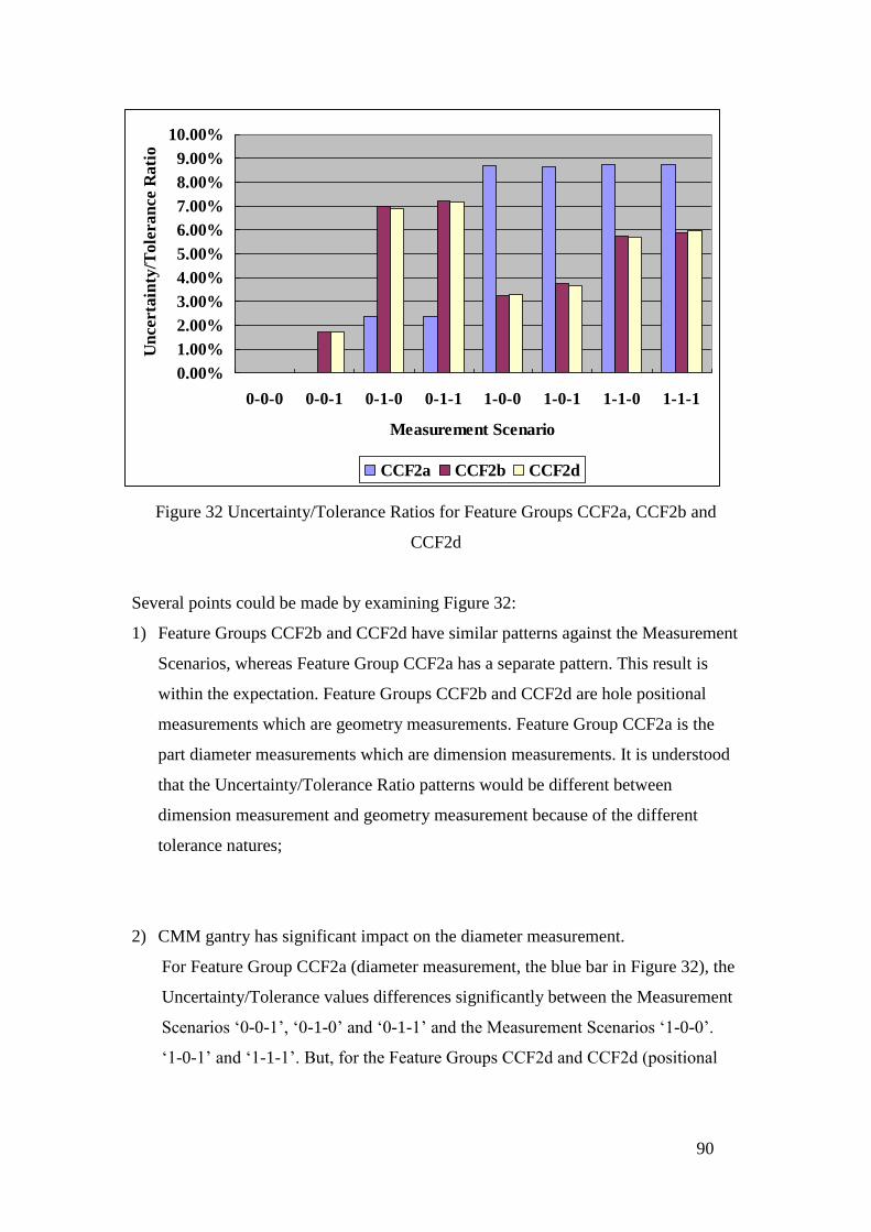
90

0.00%

1.00%

2.00%

3.00%

4.00%

5.00%

6.00%

7.00%

8.00%

9.00%

10.00%

0-0-0 0-0-1 0-1-0 0-1-1 1-0-0 1-0-1 1-1-0 1-1-1

Measurement Scenario

Un

certa

inty

/To

lera

nce R

ati

o

CCF2a CCF2b CCF2d

Figure 32 Uncertainty/Tolerance Ratios for Feature Groups CCF2a, CCF2b and

CCF2d

Several points could be made by examining Figure 32:

1) Feature Groups CCF2b and CCF2d have similar patterns against the Measurement

Scenarios, whereas Feature Group CCF2a has a separate pattern. This result is

within the expectation. Feature Groups CCF2b and CCF2d are hole positional

measurements which are geometry measurements. Feature Group CCF2a is the

part diameter measurements which are dimension measurements. It is understood

that the Uncertainty/Tolerance Ratio patterns would be different between

dimension measurement and geometry measurement because of the different

tolerance natures;

2) CMM gantry has significant impact on the diameter measurement.

For Feature Group CCF2a (diameter measurement, the blue bar in Figure 32), the

Uncertainty/Tolerance values differences significantly between the Measurement

Scenarios ‘0-0-1’, ‘0-1-0’ and ‘0-1-1’ and the Measurement Scenarios ‘1-0-0’.

‘1-0-1’ and ‘1-1-1’. But, for the Feature Groups CCF2d and CCF2d (positional

91

measurement, the purple and yellow bars in Figure 32), there is no such pattern to

be found.

The major differences between the Measurement Scenarios ‘0-0-1’, ‘0-1-0’ and

‘0-1-1’ and the Measurement Scenarios ‘1-0-0’. ‘1-0-1’ and ‘1-1-1’ are the

effectiveness of the CMM Gantry uncertainty contributor. When the CMM gantry

is effective, the uncertainty of diameter measurement (Feature Group CCF2a) is

significantly. The CMM gantry has significant effects on diameter measurement,

but not on positional measurement.

This judgement is reasonably consistent with the physical measurement

environment. For the diameter measurements, the CMM gantry needs to move

long distance due to the large scale of the part (about 3 meters in diameter).

Enormous kinematic errors have been introduced during the CMM gantry

movement. For the position measurements, the CMM gantry only needs to move

within a relatively small area to inspect the hole. Therefore, the CMM gantry has

an obvious impact on the diameter measurement uncertainty, but not on the

positional measurement uncertainty.

This analysis result suggests metrology engineers should notice the nature of a

feature when making the measurement plan, and to minimize the kinematic errors

of the CMM gantry movements especially for large-scale dimension

measurements.

3) Probe has lowest impact on the measurement uncertainty.

The Uncertainty/Tolerance Ratio is at the lowest on Measurement Scenario 0-0-1,

where only ‘Probe’ contributor is effective. In particular, the

Uncertainty/Tolerance Ratio value becomes nil on Measurement Scenario for the

Feature Group CCF2a (diameter measurement). The low measurement

uncertainty value and the relatively high tolerance value round up the Ratio value

to nil. It indicates that the Probe is not a significant factor for the large-scale

diameter measurement in this case.

92

This judgement is consistent with the common understanding on the physical

measurement process. Given this judgement, metrology engineers could

potentially save capital investment on purchasing better probes, and focus on

improving the CMM gantry movements and temperature control.

4) Two non-normative patterns have been realized from Figure 32.

Firstly, it is expect that the Uncertainty/Tolerance Ratio reaches a peak value at

the Measurement Scenario 1-1-1 where all of the three measurement uncertainty

contributors are effective. However, for the Feature Groups CCF2b and CCF2d

(positional measurement), the peak value of the Uncertainty/Tolerance Ratio

appears at the Measurement Scenario 0-1-1. This non-normative pattern reflects

the incapability of predicting the geometry measurement uncertainty in the digital

environment. The complexity of the geometry measurement is a crucial challenge

for measurement process modelling and measurement uncertainty estimation.

Secondly, the Temperature factor has little effect on the Feature Group CCF2a

(diameter measurement). For example, the value of the Uncertainty/Tolerance

Ratio of the Feature Group CCF2a (the blue bars in Figure 32) changes little

between the Measurement Scenario 1-0-1 and the Measurement Scenario 1-1-1,

the difference of which is the effectiveness of the Temperature factor. This digital

measurement result counters common understandings on thermal expansion rules,

and remains unexplainable. It indicates that the performance of the digital CMM

model still needs to be improved, especially for the large-scale measurement and

complex feature inspection.

Conclusively speaking, the reliability of the digital measurement results is critiqued

again. Due to the availability of the physical measurement resources, it is difficult to

design and perform an extra set of physical measurements to confirm the above

judgments. However, it indicates an alternative way of utilizing the digital CMM

measurement model, of which result can justify the impacts of measurement

uncertainty contributors. The digital measurement uncertainty can have sensible

applications to physical measurement, if the digital measurement uncertainty analysis

could be analyzed and examined in more sophisticated approach.

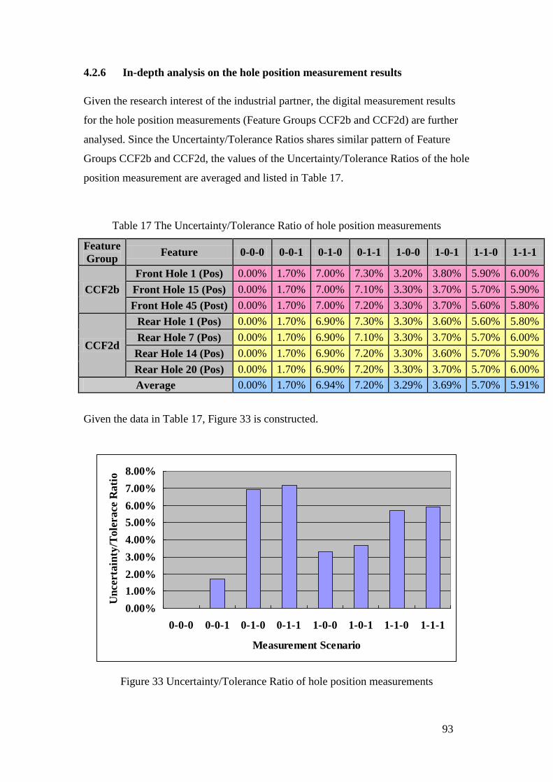
93

4.2.6 In-depth analysis on the hole position measurement results

Given the research interest of the industrial partner, the digital measurement results

for the hole position measurements (Feature Groups CCF2b and CCF2d) are further

analysed. Since the Uncertainty/Tolerance Ratios shares similar pattern of Feature

Groups CCF2b and CCF2d, the values of the Uncertainty/Tolerance Ratios of the hole

position measurement are averaged and listed in Table 17.

Table 17 The Uncertainty/Tolerance Ratio of hole position measurements

Feature

Group Feature 0-0-0 0-0-1 0-1-0 0-1-1 1-0-0 1-0-1 1-1-0 1-1-1

CCF2b

Front Hole 1 (Pos) 0.00% 1.70% 7.00% 7.30% 3.20% 3.80% 5.90% 6.00%

Front Hole 15 (Pos) 0.00% 1.70% 7.00% 7.10% 3.30% 3.70% 5.70% 5.90%

Front Hole 45 (Post) 0.00% 1.70% 7.00% 7.20% 3.30% 3.70% 5.60% 5.80%

CCF2d

Rear Hole 1 (Pos) 0.00% 1.70% 6.90% 7.30% 3.30% 3.60% 5.60% 5.80%

Rear Hole 7 (Pos) 0.00% 1.70% 6.90% 7.10% 3.30% 3.70% 5.70% 6.00%

Rear Hole 14 (Pos) 0.00% 1.70% 6.90% 7.20% 3.30% 3.60% 5.70% 5.90%

Rear Hole 20 (Pos) 0.00% 1.70% 6.90% 7.20% 3.30% 3.70% 5.70% 6.00%

Average 0.00% 1.70% 6.94% 7.20% 3.29% 3.69% 5.70% 5.91%

Given the data in Table 17, Figure 33 is constructed.

0.00%

1.00%

2.00%

3.00%

4.00%

5.00%

6.00%

7.00%

8.00%

0-0-0 0-0-1 0-1-0 0-1-1 1-0-0 1-0-1 1-1-0 1-1-1

Measurement Scenario

Un

certa

inty

/To

lera

ce R

ati

o

Figure 33 Uncertainty/Tolerance Ratio of hole position measurements

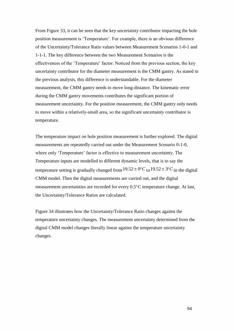
94

From Figure 33, it can be seen that the key uncertainty contributor impacting the hole

position measurement is ‘Temperature’. For example, there is an obvious difference

of the Uncertainty/Tolerance Ratio values between Measurement Scenarios 1-0-1 and

1-1-1. The key difference between the two Measurement Scenarios is the

effectiveness of the ‘Temperature’ factor. Noticed from the previous section, the key

uncertainty contributor for the diameter measurement is the CMM gantry. As stated in

the previous analysis, this difference is understandable. For the diameter

measurement, the CMM gantry needs to move long-distance. The kinematic error

during the CMM gantry movements contributes the significant portion of

measurement uncertainty. For the position measurement, the CMM gantry only needs

to move within a relatively-small area, so the significant uncertainty contributor is

temperature.

The temperature impact on hole position measurement is further explored. The digital

measurements are repeatedly carried out under the Measurement Scenario 0-1-0,

where only ‘Temperature’ factor is effective to measurement uncertainty. The

Temperature inputs are modelled to different dynamic levels, that is to say the

temperature setting is gradually changed from C 052.19 to C 352.19 in the digital

CMM model. Then the digital measurements are carried out, and the digital

measurement uncertainties are recorded for every 0.5C temperature change. At last,

the Uncertainty/Tolerance Ratios are calculated.

Figure 34 illustrates how the Uncertainty/Tolerance Ratio changes against the

temperature uncertainty changes. The measurement uncertainty determined from the

digital CMM model changes literally linear against the temperature uncertainty

changes.

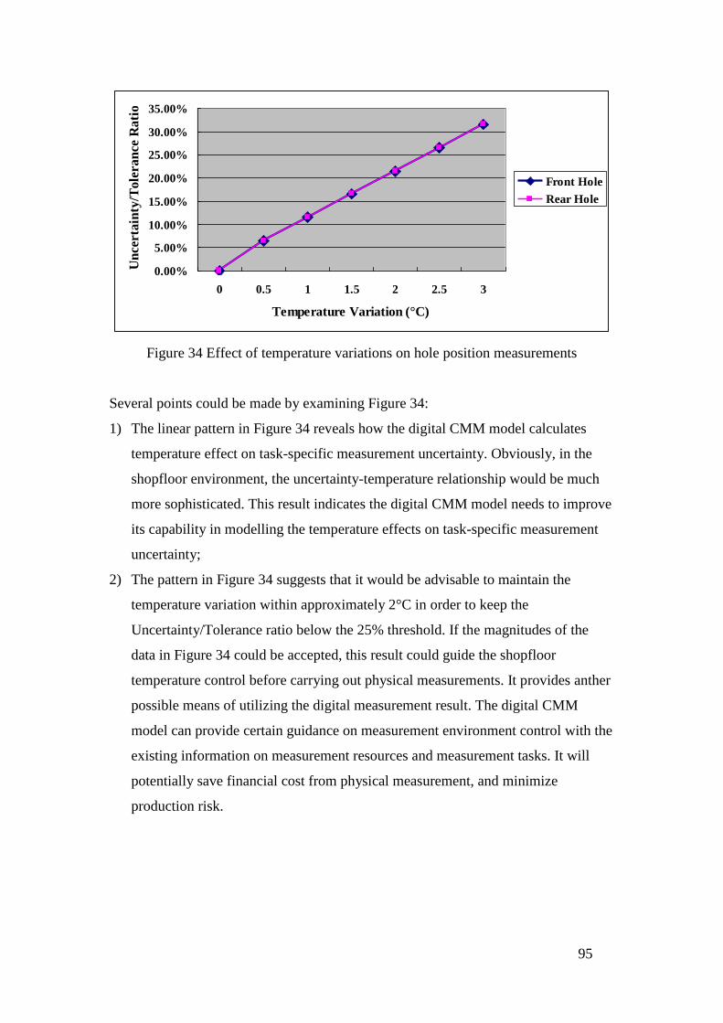
95

0.00%

5.00%

10.00%

15.00%

20.00%

25.00%

30.00%

35.00%

0 0.5 1 1.5 2 2.5 3

Temperature Variation (°C)

Un

certa

inty

/Tole

ran

ce R

ati

o

Front Hole

Rear Hole

Figure 34 Effect of temperature variations on hole position measurements

Several points could be made by examining Figure 34:

1) The linear pattern in Figure 34 reveals how the digital CMM model calculates

temperature effect on task-specific measurement uncertainty. Obviously, in the

shopfloor environment, the uncertainty-temperature relationship would be much

more sophisticated. This result indicates the digital CMM model needs to improve

its capability in modelling the temperature effects on task-specific measurement

uncertainty;

2) The pattern in Figure 34 suggests that it would be advisable to maintain the

temperature variation within approximately 2°C in order to keep the

Uncertainty/Tolerance ratio below the 25% threshold. If the magnitudes of the

data in Figure 34 could be accepted, this result could guide the shopfloor

temperature control before carrying out physical measurements. It provides anther

possible means of utilizing the digital measurement result. The digital CMM

model can provide certain guidance on measurement environment control with the

existing information on measurement resources and measurement tasks. It will

potentially save financial cost from physical measurement, and minimize

production risk.

96

4.2.7 Summary

The pilot study carried above is a useful exercise for learning about the potential

benefits and challenges of using the digital CMM model to predict task-specific

measurement uncertainty and analyze the CMM measurement capability.

In order to verify the performance of the digital CMM model, the physical

measurement environment has been established as identical as possible to the digital

measurement environment. Then the physical measurements have been carried out on

a large-scale component by measuring its dimension and geometry features. The

physical measurement results are compared with the digital measurement results.

Since the comparison results do not fully convince the performance of the digital

CMM model, extra set of experiments are carried out to explore the alternative means

of using the digital CMM model. Several conclusions have been drawn.

The uncertainty obtained from the digital measurement is generally higher than that

obtained from the physical measurement. It reflects the nature of the

Simulation-by-Constraint (SBC) method, which is employed by the digital CMM

model. Since the SBC method does not require a complete description of the CMM

process, the measurement uncertainty calculated by the SBC method tends to be

higher. On the other hand, by comparing the digital measurement uncertainty with the

GUM-approach uncertainty, it shows that the digital CMM model has relatively good

consistent with the GUM instructions.

The digital measurement results vary against the feature natures. It indicates the

digital CMM model carries out feature-based uncertainty calculation algorithm for

task-specific measurement. In particularly, the digital CMM model is more capable of

‘measuring’ dimension features than geometry features;

The performance of the digital CMM model is not fully verified by the physical

measurements. Due to the high complexity and diversity of the CMM measurement

tasks, it is very difficult to provide a digital CMM model which includes all of

measurement uncertainty contributors and measurement scenarios. Moreover, it is

barely feasible to establish the physical measurement environment exactly the same as

97

the digital measurement environment. It is virtually impossible to verify the diverse

measurement tasks by physical measurements for task-specific measurement

uncertainty estimation.

The alternative applications of the digital CMM model are considered. The digital

measurement results are further analyzed to examine the impacts of the measurement

uncertainty contributors. The analysis results have shown promising perspective. By

deploying delicate experiment design and data analysis techniques, the digital

measurement uncertainty could be utilized to answer the questions such as which

measurement uncertainty contributor(s) have the most significant impact on the

overall measurement system, and consequently to guide the measurement system

design in physical environment. It indicates the next step of the research is to establish

a robust algorithm and procedures to achieve this objective.

4.3 Chapter summary

The chapter explores how to utilize the digital simulation techniques to model the

CMM measurement process in the digital environment, and to determine the

task-specific measurement result. The chapter firstly introduces a digital CMM model.

It employs the Simulation-by-Constraint (SBC) method and performs Monte-Carlo

simulation to predict CMM task-specific measurement uncertainty in the digital

environment. Then a pilot study on ‘measuring’ a large-scale part in the digital CMM

model has been carried out. The simulation measurement results have been compared

with the physical measurement results to verify the performance the digital CMM

model. Through the verification work, the strengths and the limitations of the digital

CMM model have been explored. Further research on utilizing the digital

measurement results has been suggested.

98

Chapter 5 A Measurement Planning and Implementation

Framework to Compare Digital and Physical Measurement

Uncertainty

5.1 Introduction

Task-specific measurement uncertainty plays an important role in the CMM

measurement evaluation. Various digital CMM models have been developed to

predict the task-specific measurement uncertainty before carrying out physical

measurement. However, as concluded from the inspection study in Chapter 4, the

performance of the digital CMM model is not fully verified. The digital measurement

result depends highly on the inputs of measurement uncertainty contributors. The

closeness between the digital and physical measurement results remains inconclusive.

Moreover, it is virtually impossible to validate the simulation results under all of the

measurement scenarios due to the variety of CMM measurement tasks. The effective

integration between digital and physical measurement environments challenges both

of the simulation software developer and the end-user.

A pilot study has been carried out using Design of Experiments (DOE) method to

statistically analyze the simulation uncertainty and inform the integration between

digital and physical environments. Based on the pilot study, this chapter proposes a

novel measurement planning and implementation framework which employs the DOE

method. The framework serves for the post-measurement data analysis and evaluation,

aiming to provide closer integration between the digital and physical measurement

environments.

The Chapter firstly identifies the limitations of the CMM digital model for evaluating

task-specific measurement uncertainty. Then the design of a generic framework to

analyze the simulation uncertainty is introduced. The details of the modules of the

framework are explained in the following section. At last, the implementation of the

framework is provided to prove the integration between the digital measurement

environment and the physical measurement environment.

99

5.2 The limitations of task-specific uncertainty simulation model

The literature reviewed in Chapter 2 has pointed out the limitations of using

simulation techniques to evaluate the task-specific measurement uncertainty. The pilot

study has provided first-hand experience to realize the limitations of the CMM digital

model. From the literature review and the pilot studies, we summarize the difficulties

of verifying the performance of the CMM digital model, and align these difficulties

under the stages of verifying the CMM digital model as shown in Figure 35. The

stages of verification work include the ‘CMM digital model’ itself, ‘running the CMM

digital model’ and ‘verifying the performance of the CMM digital model’. The

difficulties of each simulation stage are further explained in Figure 35.

Simulation Stage Difficulty of Each stage

Digital CMM model

Running the digital CMM

model

It is difficult to conclude all of the

measurement uncertainty contributors into

the algorithm of a CMM digital model.

It is difficult to model the uncertainty

contributors in the right way, while the

simulation result of the CMM digital model

highly relies on the quality of the uncertainty

contributor inputs

Verifying the

performance of digital

CMM model

1) It is virtually impossible to verify all of the

simulation measurement scenarios in the

physical experiments;

2) It is difficult to know the uncertainty

reported by the digital CMM model is due to

the measurement uncertainty contributors or

due to a correct use of limited information.

Figure 35 Limitations of the CMM digital model

To conclude, the difficulties of verifying the CMM digital model are due to the

contradiction between the nature of task-specific measurement uncertainty and the

100

large diversity of the CMM measurement tasks. It is nearly impossible to simulate all

of the scenarios of the task-specific measurements in the digital measurement

environment The difficulties limit the development of evaluating task-specific

measurement uncertainty in digital environment.

5.3 Examining uncertainty contributor effects by using Design of

Experiments (DOE) approach

Given the limitations described in the previous section, the Design of Experiment

(DOE) approach is considered to explore whether the simulation results can be used

in statistical analysis for alternative purposes. A trial study has been carried out. The

trial study statistically analyzes the simulation results aiming to make a technical

contribution to decision-making through the quantification of uncertainties in the

relevant variables. The classical statistical approach, Design of Experiments (DOE),

is adopted in the trial study to process the post-measurement data given by the

simulation software. It aims to quantitatively evaluate which uncertainty contributors

have the biggest impact on the entire measurement system performance.

In order to determine the task-specific measurement uncertainty, a slotted block is

loaded in the digital CMM model (Figure 36). The 30mm-diameter shallow hole on

the slotted block is “measured”. The digital CMM model evaluates the measurement

uncertainties of the diameter and position of the shallow hole (as denoted in Figure

36).

101

Figure 36 The artefact and measured features

A full factorial design* is carried out. Three factors influencing the CMM

measurement uncertainty are selected; they are CMM Specification, Environment and

Probing Strategy respectively. Each of the factors is designed to have three levels.

The details of the factors and the factorial levels are listed in Table 18. One

combination of the random factorial levels is called a ‘measurement scenario’. For a

full-factorial experiment, there are 2733 measurement scenarios.

* In statistics, a full factorial experiment is an experiment whose design consists of two or more factors, each with

discrete possible values or "levels", and whose experimental units take on all possible combinations of these levels

across all such factors.

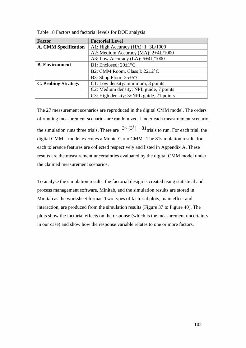
102

Table 18 Factors and factorial levels for DOE analysis

Factor Factorial Level

A. CMM Specification A1: High Accuracy (HA): 1+3L/1000

A2: Medium Accuracy (MA): 2+4L/1000

A3: Low Accuracy (LA): 5+4L/1000

B. Environment B1: Enclosed: 201C

B2: CMM Room, Class I: 222C

B3: Shop Floor: 255C

C. Probing Strategy C1: Low density: minimum, 3 points

C2: Medium density: NPL guide, 7 points

C3: High density: 3NPL guide, 21 points

The 27 measurement scenarios are reproduced in the digital CMM model. The orders

of running measurement scenarios are randomized. Under each measurement scenario,

the simulation runs three trials. There are 81)3(3 3 trials to run. For each trial, the

digital CMM model executes a Monte-Carlo CMM . The 81simulation results for

each tolerance features are collected respectively and listed in Appendix A. These

results are the measurement uncertainties evaluated by the digital CMM model under

the claimed measurement scenarios.

To analyse the simulation results, the factorial design is created using statistical and

process management software, Minitab, and the simulation results are stored in

Minitab as the worksheet format. Two types of factorial plots, main effect and

interaction, are produced from the simulation results (Figure 37 to Figure 40). The

plots show the factorial effects on the response (which is the measurement uncertainty

in our case) and show how the response variable relates to one or more factors.

103

LAMAHA

3.0

2.5

2.0

1.5

1.0

Shop FloorCMM RoomEnclosure

3*NPLNPLMinimum

3.0

2.5

2.0

1.5

1.0

CMM Specification

Me

an

Environment

Probing Strategies

Main Effects Plot for Diameter_01Data Means

Figure 37 Main effects plot for position measurement

Shop FloorCMM RoomEnclosure 3*NPLNPLMinimum

3

2

1

3

2

1

CMM Specification

Environment

Probing Strategies

HA

MA

LA

Specification

CMM

Enclosure

CMM Room

Shop Floor

Environment

Interaction Plot for Diameter_01Data Means

Figure 38 Interaction plot for diameter measurement

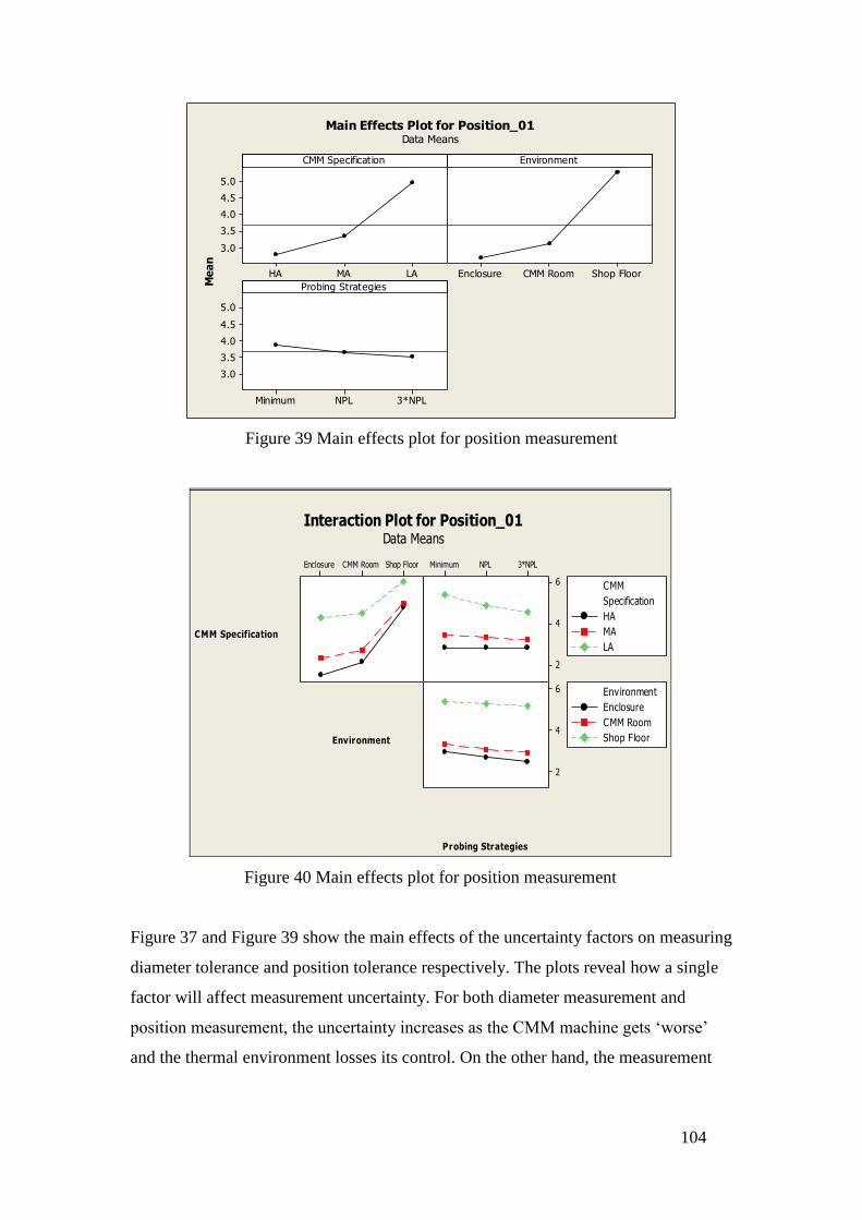
104

LAMAHA

5.0

4.5

4.0

3.5

3.0

Shop FloorCMM RoomEnclosure

3*NPLNPLMinimum

5.0

4.5

4.0

3.5

3.0

CMM Specification

Me

an

Environment

Probing Strategies

Main Effects Plot for Position_01Data Means

Figure 39 Main effects plot for position measurement

Shop FloorCMM RoomEnclosure 3*NPLNPLMinimum

6

4

2

6

4

2

CMM Specification

Environment

Probing Strategies

HA

MA

LA

Specification

CMM

Enclosure

CMM Room

Shop Floor

Environment

Interaction Plot for Position_01Data Means

Figure 40 Main effects plot for position measurement

Figure 37 and Figure 39 show the main effects of the uncertainty factors on measuring

diameter tolerance and position tolerance respectively. The plots reveal how a single

factor will affect measurement uncertainty. For both diameter measurement and

position measurement, the uncertainty increases as the CMM machine gets ‘worse’

and the thermal environment losses its control. On the other hand, the measurement

105

uncertainty decreases as the sampling points are intensified. The results are in

accordance with the general rules of measurement practice.

Moreover, Figure 37 and Figure 39 show the influence power of the uncertainty

factors in a quantitative way. For example, for the diameter measurement in Figure

37, the variability of main effect for the Environment factor is significantly bigger

than the ones for the CMM Specification factor and the Probing Strategy factor. It

suggests that the thermal environment has a greater influence on measurement

uncertainty than the other uncertainty factors. By further comparison, we can rank the

influence powers of the uncertainty factors as below:

"_""_""" PowerSamplingionSpecificatCMMtEnvironmen

This analytical result is consistent with the experiences of CMM measurement experts.

It quantitatively shows how to control the uncertainty factors in order to minimize the

measurement uncertainty. So when facing multiple yet limited choices of improving

CMM measurement process, measurement engineers can reference the analytical

result, and then decide how to control the measurement uncertainty contributors.

Figure 38 and Figure 40 respectively show the interactions of the uncertainty factors

on measuring the diameter and the position. The interaction plots display the

combined effects of the two factors on the measurement uncertainty. They provide the

comparison between two uncertainty factors without accounting the third factor’s

effect, and hence give further guidance to measurement engineers to prioritize the

choices of improving CMM inspection systems.

The Figure 38 and Figure 40 also show that thermal environment has the greatest

influence on the measurement uncertainty. Additionally, more details of the factorial

influences are shown up. For example, by examining the combined effect of CMM

Specification and Sampling Strategy (in the top right box in ), it can be concluded that

the Sampling Strategy has very small effect on the measurement uncertainty when

using a high-accuracy CMM machine, while still having a clear impact when using a

low-accuracy CMM. It suggests that when using a high-accuracy CMM, the number

of sampling points can be reduced, which consequently saves measurement time and

improves production efficiency.

106

Although Figure 38 and Figure 40 indicate similar trends, there are still nuances

exhibited in the two figures. The nature of the tolerance feature also has effect on the

measurement uncertainty. For example, the three curves in the top right box in Figure

38 get very close at the end. These curves represent the combined effect of CMM

Specification and Sampling Strategy when measuring the diameter. It suggests that

for the diameter measurement, improving the number of sampling points can reduce

the measurement uncertainty to a level close to which by improving the accuracy of

CMM machine. The same effect does not reveal in the case of position measurement

(the top right box in Figure 40). Measurement engineers need to take into account the

types of features of the part, and then decide to purchase a new CMM machine or

simply improve the sampling strategy.

The initial DOE analysis of the simulation results has shown promising results. The

analysis results have certain logic coherence with the common understanding on

CMM measurement process. Given the DOE analysis results, a framework to

integrate the digital and physical environments is proposed in the next section.

5.4 Design of a generic framework to compare digital and physical

measurement environments

The contradiction between the nature of task-specific measurement uncertainty and

the diversity of CMM measurement tasks prevents the integration of digital and

physical measurement environments. To solve the problem, a generic framework, is

proposed, aiming to compare the two measurement environments (as shown in Figure

41). The framework employs Design of Experiments (DOE) techniques to process the

post-measurement data sets, and evaluates the influence of measurement uncertainty

contributors.

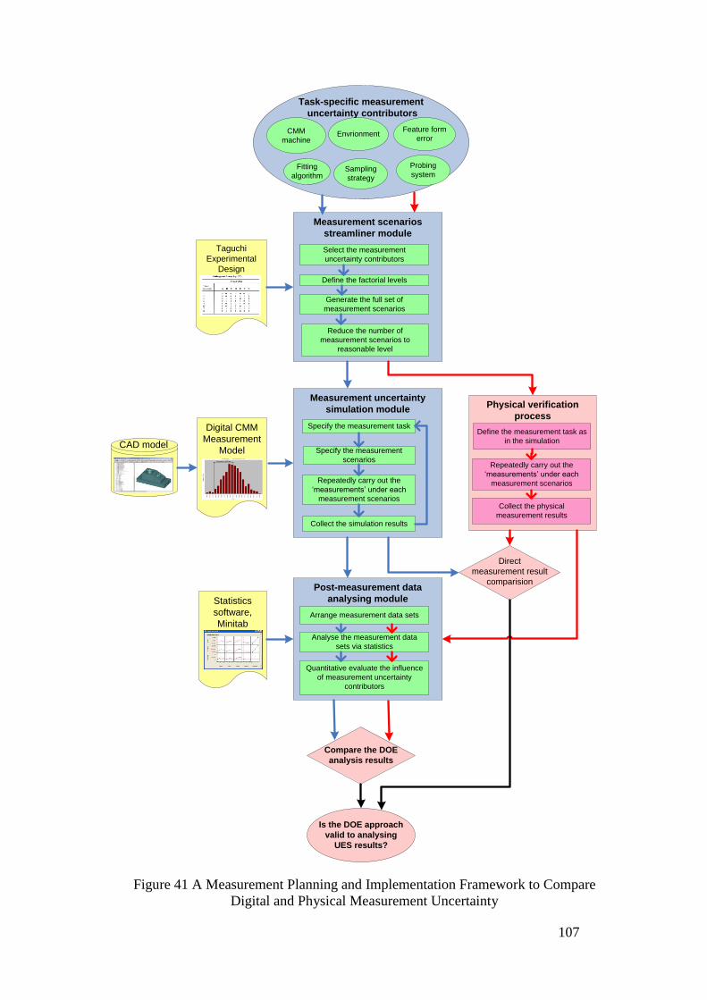
107

Task-specific measurement

uncertainty contributors

Taguchi

Experimental

Design

Measurement scenarios

streamliner module

Select the measurement

uncertainty contributors

Generate the full set of

measurement scenarios

Reduce the number of

measurement scenarios to

reasonable level

Define the factorial levels

Measurement uncertainty

simulation module

Post-measurement data

analysing module

Repeatedly carry out the

‘measurements’ under each

measurement scenarios

Specify the measurement task

Specify the measurement

scenarios

Collect the simulation results

Digital CMM

Measurement

ModelCAD model

Analyse the measurement data

sets via statistics

Arrange measurement data sets

Statistics

software,

Minitab

Quantitative evaluate the influence

of measurement uncertainty

contributors

Physical verification

process

CMM

machine Envrionment

Probing

systemFitting

algorithmSampling

strategy

Feature form

error

Define the measurement task as

in the simulation

Repeatedly carry out the

‘measurements’ under each

measurement scenarios

Collect the physical

measurement results

Direct

measurement result

comparision

Compare the DOE

analysis results

Is the DOE approach

valid to analysing

UES results?

Figure 41 A Measurement Planning and Implementation Framework to Compare

Digital and Physical Measurement Uncertainty

108

As shown in Figure 41, the entire framework is composed of three domains, which are

the digital measurement environment (blue in Figure 41), the physical measurement

environment (red in Figure 41) and the external resources (yellow in Figure 41)

respectively. The blue arrows represent the operations flow in the digital environment,

while the red arrows represent the operations flow in the physical environment. The

details of the digital and physical measurement flows and the comparison methods are

described separately in the following sub-sections.

5.4.1 The ‘Task-specific Measurement Uncertainty Contributors’

The working flow starts from collecting the measurement uncertainty contributors.

Six major uncertainty contributors are considered by the digital CMM model. These

uncertainty contributors include CMM machine, thermal environment, feature form

error, probing system, sampling strategy and fitting algorithm.

5.4.2 The ‘Measurement Scenario Streamliner’ module

The ‘Measurement Scenario Streamliner’ module collects the measurement

uncertainty contributors. The end-user can select the uncertainty contributors (control

factors) needed and define their factorial levels given the measurement aim. The

combinations of the selected uncertainty contributors and their factorial levels create a

full set of measurement scenarios.

The ‘Taguchi Orthogonal Array’ (shown in yellow in Figure 41) is deployed in the

‘Measurement Scenario Streamliner’ model to reduce the number of measurement

scenarios to a reasonable level. The Taguchi DOE method and its implementation are

described in sub-sections 5.5.2 and 5.6.1.

The ‘Measurement Scenario Streamliner’ module outputs the measurement scenarios,

given which the digital and physical measurements are carried out. After the

‘Measurement Scenario Streamliner’ module, the measurements are carried out

respectively in the digital measurement environment and the physical measurement

environment, where the task-specific measurement uncertainties are obtained.

109

5.4.3 The ‘Measurement Uncertainty Simulation’ module

The ‘Measurement Uncertainty Simulation’ module represents the measurements

carried out in digital environment.

The Module receives measurement scenarios information from the ‘Measurement

Scenario Streamliner’ module. Meanwhile, it perceives the feature-based design

information from the product CAD-model, and employs a standing-alone digital

CMM model to calculate the task-specific measurement uncertainty (shown in yellow

in Figure 41).

The Module integrates the above information, and allows the end-user to define the

details of digital measurements. Measurement tasks are specified given product design

information, and measurement scenarios are further clarified in the digital CMM

model. Then digital measurements are repeatedly carried out under each

measurement scenario. The digital measurement simulates CMM measurement

process and runs Monte-Carlo simulation. The output of the Module is a set of the

task-specific measurement uncertainty calculated by the digital CMM model under

the selected measurement scenarios.

5.4.4 The ‘Physical Verification Process’

The ‘Physical Verification Process’ module represents the CMM measurements which

are carried out in physical environment. The physical measurements are carried out

as close as in the digital environment. Therefore, the Physical Verification Process

includes similar operations as in the ‘Measurement Uncertainty Simulation’ module.

The Physical Verification Process includes:

Define measurement task as in the digital environment;

Repeatedly carry out measurements under each measurement scenario;

Collect the physical measurement results.

The output of the ‘Physical Verification Process’ is a set of measurement

uncertainties of selected measurement scenarios in the physical measurement

environment..

110

Both of the digital and physical measurement results are collected for comparison and

verification.

5.4.5 The ‘Post-Measurement Data Analyzing’ module

The ‘Post-Measurement Data Analyzing’ module receives the measurement result

data sets from both of digital measurements and physical measurements.

The Module collects the measurement results from the digital or physical

environments. It employs professional statistics software, Minitab, to run the Design

of Experiments (DOE) analysis, and obtains the DOE analysis results of the digital

measurement and physical measurement respectively. The details of DOE method

and implementation are described in subsections 5.5.2 and 5.6.3.

The outputs of the Module are a set of main effect plots, which represent influence

levels of uncertainty contributors for the defined measurement task.

5.4.6 Comparison

In order to verify the simulation performance, the digital and physical measurement

results are compared. Noticeably, there are two sets of measurement results obtained

from the above measurement activities. One is the direct measurement results, and the

other one is the DOE analysis results. The comparison of direct measurement results

assesses the capability of the digital CMM model in predicting the task-specific

measurement uncertainty. The comparison of DOE analysis results assesses the

capability of the DOE approach on evaluating the influence of measurement

uncertainty contributors. Consequently, it provides the verification of the digital

CMM measurement model in the physical environment.

The digital and physical operation flows are described in details in the next two

sections respectively.

111

5.5 Overview of framework methodologies

The measurement planning and implementation framework described in Section 5.4 is

a robust framework deployed with several methodologies in metrology, statistics and

software engineering. In this section, the principles of these methodologies are

explained and further introduced.

5.5.1 Task-specific measurement uncertainty contributors

Task-specific measurement uncertainty is the measurement uncertainty of measuring a

specific feature using a specific measurement strategy [13]. The definition of

‘task-specific measurement uncertainty’ addresses the traceability of measurement,

and consequently facilitates the importance of the measurement uncertainty

contributors. To determine the measurement uncertainty, it is vital to indentify the

measurement uncertainty contributors prior to executing measurement.

In our research, we have considered six measurement uncertainty contributors, which

are CMM machine, environment (temperature), feature form error, fitting algorithm,

sampling strategy and probing system respectively. There are 4 reasons of selecting

these measurement uncertainty contributors:

Importance: these six factors have significant influence on CMM measurement

uncertainty;

Independence: the six factors are relatively independent from each other*;

Operation: the effects of the six factors can be validated in the laboratory

environment;

Manageable: the selection of the six factors is consistent with the research focus

and expertise.

It is noticeable that the selection of measurement uncertainty contributors is

expandable. The selection can be beyond the ones proposed. The CMM measurement

planning and implementation framework proposed in this research is expected to be

applicable in more sophisticated measurement scenarios which includes a broader

diverse of measurement uncertainty factors.

* The independence of the factors will be quantitatively analyzed.

112

5.5.2 ‘Measurement Scenario Streamliner’ module: Taguchi experimental

design

‘Taguchi experimental design’ is deployed in the ‘Measurement Scenario Streamliner’

module. In classically designed experiments, the primary goal is to identify factors

that affect the mean response and control them to desirable levels. Taguchi focuses on

reducing variability, as well as setting the mean to target.

In Taguchi design of experiments, the control factors and their factorial levels are

firstly defined. The combination of the control factor and the factorial levels settings

produce a large number of experimental scenarios, which is possibly too high to be

practiced in the laboratory environment. To reduce the number of experimental runs,

the Taguchi Orthogonal Array is used.

The ‘Taguchi orthogonal arrays’ is a methodology of designing experiments that

usually requires only a fraction of the full factorial combinations. Figure 42 shows a

‘Taguchi Orthogonal Array Selector’. The column of ‘Taguchi Orthogonal Array

Selector’ is the number of experimental factors, and the row is the number of factorial

levels.

113

Figure 42 Taguchi Orthogonal Array Selector [132]

114

Given to experimental factors selected, their factorial levels and ‘Taguchi Orthogonal

Array Selector’, an appropriate orthogonal array is selected. Each column in the

orthogonal array represents a specific factor with two or more levels. Each row

represents a run; the cell values indicate the factor settings for the run. An orthogonal

array allows the design to be balanced so that factor levels are weighted equally.

Because of this, each factor can be evaluated independently of all the other factors, so

the effect of one factor does not influence the estimation of another factor [132].

An example of Taguchi design of experiment is given in Appendix B.

5.5.3 Measurement Uncertainty Simulation module: the

simulation-by-constraints method

The simulation-by -constraints method is deployed in the Digital CMM model, which

allows the ‘Measurement Uncertainty Simulation’ module to generate measurement

uncertainty. The simulation-by-constraints method has been reviewed in the Chapter 2

– Literature Review as one of four major simulation methods for evaluating

task-specific measurement uncertainty.

The simulation-by-constraints method starts with populating a large amount of virtual

CMMs, each of which has a random error state. Each virtual CMM is characterized by

the 21 parametric errors. Theoretically the data sets which describe the virtual CMMs

states could be infinite. But in practice, the random error state is “limited” by physical

CMM calibrated results. For example, a CMM calibration result shows that the largest

error of measuring a calibrated step gauge along the X-axis is 10m, it is unlikely the

X-axis scalar error of the CMM machine is significantly larger than 10m.

Therefore, the large amount of virtual CMMs reasonably represents the complete state

space of the CMM. This data set, which describes the virtual CMM states, is bounded

by a bounding measurement set, which is a set of actual measurement results of

certain reference length (e.g. a step gauge). The virtual CMMs carry out

measurements on the bounding measurement set. If the virtual CMM state shows the

same errors as the complete bounding measurement set, the virtual CMM is retained.

Otherwise it is rejected. Majority of the virtual CMM states are rejected, and only a

115

few are retained. The retention rate is between 0.01% and 0.00001%. Consequently,

the bounding measurement set defines a bounded area containing ‘good CMM states’.

Each of the ‘good CMM states’ could be the true state of the CMM during

measurement process.

Figure 43 illustrates an idealized machine which has only two error sources denoted

as and respectively. ‘SBC’ is short for ‘simulation-by-constraints’, and ‘FPS’ is

short for ‘full-parametric simulation’. Figure 43 shows the bounded region resulting

from the simulation-by-constraints method is much larger than that from the

full-parametric simulation method. If a very extensive bounding measurement set is

used, the bounding region from the simulation-by-constraints method will be the same

as the one with the full-parametric method.

Figure 43 Schematic of the simulation-by-constraints method

The advantage of the simulation-by-constraints method can work with incomplete

information of the CMM, whereas the full-parametric simulation requires a complete

description of CMM state. The simulation-by-constraints method does not require a

full error-mapping of CMM machine. The only requirement is that sufficient

measurements are taken to obtain bounding measurement set.

There are three reasons why the simulation-by-constraints method is selected to be

deployed in the Measurement Planning and Implementation Framework:

The simulation-by-constraints method calculates the influences of the constraints

on task-specific measurement uncertainty. This is consistent with the expected

outcomes of Taguchi experimental design;

116

Compared to the other simulation methods, the simulation-by-constraints method

does not require full parametric error-mapping of the CMM machine, which is

time-consuming and laborious to obtain. Using the simulation-by-constraints

method in the Framework can potentially reduce the workload of the metrology

engineers, if the Framework is validated;

The simulation-by-constraints method is available in the laboratory resources.

5.6 Overview of framework implementation

The implementation of the Measurement Planning and Implementation Framework

described here has been carried out in the digital and physical environments. In the

digital environment, the Framework is implemented by using commercially-available

software to determine task-specific measurement uncertainty and generate statistical

analysis result. In the physical environment, physical measurements are carried out in

the finely-controlled testing environment in collaboration with the National Physical

Laboratory (NPL), UK. This section describes the key stages of the Framework

implementation.

5.6.1 Measurement uncertainty generation using the simulation software

The primary objective of the Framework implementation is to generate task-specific

measurement uncertainty in the digital environment. Therefore, the digital

environment needs to have the following capabilities:

Able to provide a CMM task-specific measurement simulation environment;

Able to carry out the simulation-by-constraints approach;

Able to calculate measurement uncertainty.

Given the above considerations, the SolidWorks and PUNDIT/CMM software

package have been deployed to assist the Framework implementation.

The SolidWorks (coloured in green in Figure 44) is a commercial software package

allowing feature-based design in the digital environment [133]. The workpiece

CAD-model is created in SolidWorks, and converted into DMIS-coded file allowing

the CAD-model to be accepted by the digital CMM model.

117

PUNDIT/CMM (coloured in blue in Figure 44) has a built-in database of common

CMMs. It imports the CAD-model of a workpiece, and provides options allowing the

user to establish the CMM measurement tasks, e.g. selecting a CMM, formulating

feature form error, defining measurement plan [131]. The measurement uncertainty

calculation is based on the simulation-by-constraints approach of NIST [131]. Monte

Carlo simulation is also utilized to calculate the probability distribution of the

simulated measurement results [22]*.

Given the research aim and the capability of PUNIT/CMM, the implementation plan

of the Framework is designed and shown in Figure 44. It has three domains, which are,

‘Task-specific Measurement Uncertainty Generation Flow’, ‘PUNDIT Operation

Flow’, and ‘Supporting CAD/CAM Design Software’, respectively.

The central domain of the implementation plan is the ‘Task-specific Measurement

Uncertainty Generation Flow’. It is in the centre of Figure 44 and is highlighted in red.

The aim of the central domain is to generate task-specific measurement uncertainty in

the digital environment. It has five elements repenting the key steps of CMM

measurement. Over the operation of the ‘Task-specific Measurement Uncertainty

Generation Flow’, the elements trigger the external applications, SolidWorks and

PUNDIT/CMM, to realize the functionalities. The details of the five elements are

presented in the following paragraphs.

* The working principle and operation flow of PUNDIT/CMM can be referenced from the

previous Chapter.

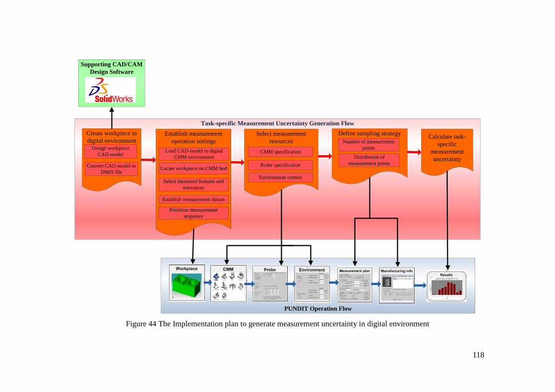
118

Task-specific Measurement Uncertainty Generation Flow

Establish measurement

operation settings

Select measurement

resources

Environment control

CMM specification

Probe specification

Define sampling strategy

Number of measurement

points

Distribution of

measurement points

Load CAD-model to digital

CMM environment

Prioritize measurement

sequence

Select measured features and

tolerances

Establish measurement datum

Locate workpiece on CMM bed

Calculate task-

specific

measurement

uncertainty

Create workpiece in

digital environmentDesign workpiece

CAD-model

Convert CAD-model to

DMIS file

Supporting CAD/CAM

Design Software

PUNDIT Operation Flow

Figure 44 The Implementation plan to generate measurement uncertainty in digital environment

119

Create workpiece in digital environment:

This element has two functions, which are to create workpiece CAD-model and to

convert the CAD-model into DMIS format. The element triggers the supporting

CAD/CAM software, the SolidWork, to realize these two functions. The

CAD-model of the measured part, including its dimension and geometry

information, is created in the SolidWork, and converted into DMIS-coded file

allowing the CAD-model to be accepted by the digital CMM model.

Establish measurement operation settings:

This element allows end-users to establish background information of

measurement operations in the digital CMM model. It has five functions, including

‘load CAD-model into the digital CMM environment’, ‘locate workpiece on CMM

bed’, ‘select measured features and tolerance’, ‘establish measurement datum’ and

‘prioritize measurement sequence’. These functions are achieved by the

‘Workpiece’ tab in PUNDIT/CMM. The workpiece CAD-model is loaded into the

PUNDIT/CMM environment, where the initial measurement operation settings are

established.

Select measurement resources:

This element allows end-users to characterize measurement resources in the digital

CMM model. It has three functions, including defining ‘CMM specification’,

‘probe specification’ and ‘environment control’ respectively. To achieve these

functions, the element triggers the CMM tab, the Probe tab and the Environment

tab in the PUNDIT/CMM. The information relating CMM measurement resources

is implemented into the digital measurement environment.

Define sampling strategy:

This element allows end-users to establish the sampling strategy on features to be

measured. It has two functions, including defining ‘number of measurement points’

and ‘distribution of measurement points’. The element triggers the Measurement

120

Plan tab and the Manufacturing Info tab to realize the above functions. The

sampling strategy of CMM measurement is implemented into the digital

measurement environment.

Calculate the task-specific measurement uncertainty:

At last, the simulation-by-constraints is performed in the digital CMM model. The

task-specific measurement uncertainty is generated in the digital environment.

5.6.2 Determining the uncertainty of physical measurements

Determining uncertainty in the physical environment is vital for verifying the digital

part of the Measurement Planning and Implementation Framework. To ensure the

scientific correctness of the physical measurement results, the physical measurement

experiments are designed and executed in collaboration with the metrology scientists

from National Physical Laboratory (NPL), where the measurement environments are

finely controlled, and the measurement instruments are deliberately calibrated and

maintained (Figure 45).

Figure 45 Finely-controlled measurement environment in NPL [134]

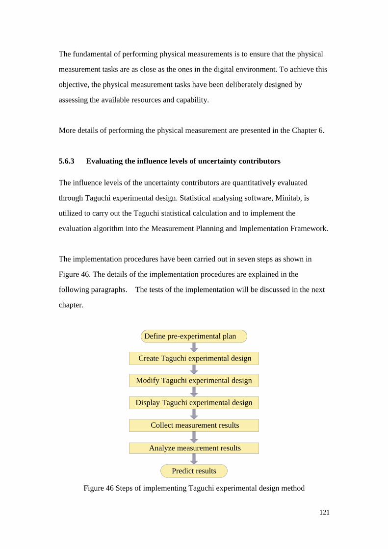
121

The fundamental of performing physical measurements is to ensure that the physical

measurement tasks are as close as the ones in the digital environment. To achieve this

objective, the physical measurement tasks have been deliberately designed by

assessing the available resources and capability.

More details of performing the physical measurement are presented in the Chapter 6.

5.6.3 Evaluating the influence levels of uncertainty contributors

The influence levels of the uncertainty contributors are quantitatively evaluated

through Taguchi experimental design. Statistical analysing software, Minitab, is

utilized to carry out the Taguchi statistical calculation and to implement the

evaluation algorithm into the Measurement Planning and Implementation Framework.

The implementation procedures have been carried out in seven steps as shown in

Figure 46. The details of the implementation procedures are explained in the

following paragraphs. The tests of the implementation will be discussed in the next

chapter.

Define pre-experimental plan

Create Taguchi experimental design

Modify Taguchi experimental design

Display Taguchi experimental design

Collect measurement results

Analyze measurement results

Predict results

Figure 46 Steps of implementing Taguchi experimental design method

122

Define pre-experimental plan:

Prior to carrying out the experiment, a plan is defined. The plan includes the

control factors and their factorial levels. The uncertainty contributors are selected

as the control factors in Taguchi experimental design, and their factorial levels are

defined given to the measurement environments and the measurement tasks. The

combinations of control factors and their factorial levels create a set of

measurement scenarios.

Create Taguchi experimental design:

In order to streamline the number of measurement scenarios, Taguchi experiment

design is created as shown in Figure 47. The appropriate Taguchi orthogonal array

is selected given to the number of control factors and the factorial levels defined in

the previous step.

Figure 47 Create Taguchi experimental design

Modify Taguchi experimental design:

The Taguchi experimental design is further modified as shown in Figure 48. The

control factors are assigned to the names of the selected measurement uncertainty

contributors of the CMM measurement tasks. The values of the factorial level are

added to the existing control factors.

123

Figure 48 Modify Taguchi experimental design

Display Taguchi experimental design:

Then the Taguchi experiment design is generated in the statistical software, as

shown in Figure 49. The streamlined measurement scenarios are displayed as a

Minitab worksheet. The rows of the worksheet show the uncertainty contributors,

and the columns show the settings of the measurement scenarios after being

applied Taguchi Orthogonal Arrays.

Figure 49 Display Taguchi experimental design

Collect measurement results:

The digital measurements are performed in the digital CMM mode. The

measurement results are collected, and then entered into the Minitab worksheet as

shown in Figure 50. These measurement results are the task-specific measurement

124

uncertainties attained from the digital or physical measurements. The worksheet is

stored in data collection for the uncertainty analysis.

Figure 50 Collect the data

Analyze measurement results:

After collecting experiment data, the measurement results are analysed as shown in

Figure 51. The analysis generates main effects and interaction plots of the S/N

ratios, means versus the control factors, and displays response tables and linear

model results for S/N ratios and means.

Figure 51 Analyze the data

125

Predict results:

Finally analysis results are generated. Analysis results indicate influence levels of

uncertainty contributors, and how the factors affecting the measurement process

are determined

By following the above steps, the algorithm which evaluates the influence levels of

measurement uncertainty contributors is implemented into the Measurement Planning

and Implementation Framework.

5.7 Chapter summary

The integration between digital and physical measurement environments is a critical

challenge for the CMM measurement planning and modelling. The complexity of the

CMM measurement tasks encounters against the fundamental concept of task-specific

uncertainty simulation model.

In this chapter, the limitations of the task-specific uncertainty simulation model have

been discussed. A full-factorial design has been performed to quantitatively compare

the influences of the uncertainty factors. Though not being scientifically verified in

the physical measurements, the DOE analysis results reveal certain agreement with

the physical CMM measurement reality. Based on this, a Measurement Planning and

Implementation Framework is proposed to analyze and integrate digital and physical

measurement uncertainty. The mathematical modelling methodologies deployed in

the Framework are deliberately investigated and extensively described. The details of

implementation of individual modules of the Framework are presented.

126

Chapter 6 Experimental Work to Validate the Framework

The Measurement Planning and Implementation Framework has been proposed in the

Chapter 5. It is a theoretical framework aiming to provide closer integration between

digital and physical measurement environments. In this chapter, the step by step

implementation of the proposed framework will be described. The experimental

work is designed and performed to validate the theoretical framework.

6.1 Overall experiment plan

Given the aim and procedures of the Measurement Planning and Implementation

Framework, this validation work has been designed. A set of experiments has been

planned, and the overall experiment plan is presented in Figure 52.

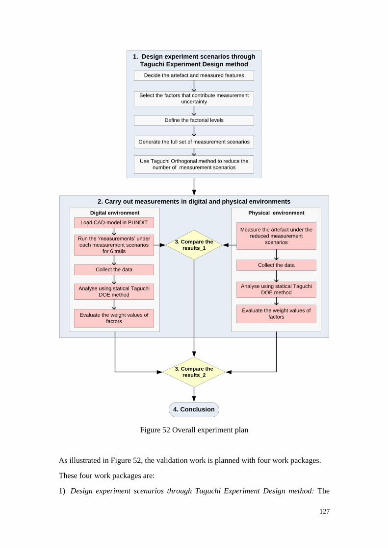
127

1. Design experiment scenarios through

Taguchi Experiment Design method

Select the factors that contribute measurement

uncertainty

Generate the full set of measurement scenarios

Use Taguchi Orthogonal method to reduce the

number of measurement scenarios

2. Carry out measurements in digital and physical environments

Define the factorial levels

Digital environment Physical environment

Decide the artefact and measured features

Load CAD-model in PUNDIT

Run the ‘measurements’ under

each measurement scenarios

for 6 trails

Analyse using statical Taguchi

DOE method

Evaluate the weight values of

factors

Measure the artefact under the

reduced measurement

scenarios

Collect the data

Analyse using statical Taguchi

DOE method

Evaluate the weight values of

factors

Collect the data

3. Compare the

results_1

3. Compare the

results_2

4. Conclusion

Figure 52 Overall experiment plan

As illustrated in Figure 52, the validation work is planned with four work packages.

These four work packages are:

1) Design experiment scenarios through Taguchi Experiment Design method: The

128

part is created, and features to be measured are selected. The measurement

uncertainty contributors are identified, which are ‘probe specification’, ‘number of

probing points’, ‘distribution of probing points’ and ‘part location’. Each of the

measurement uncertainty contributors are assigned with three factorial levels. The

combination of measurement uncertainty contributors and the factorial levels

produces a large number of measurement scenarios. The appropriate measurement

scenarios are selected by applying the Taguchi Orthogonal Array method.

2) Carry out measurements in the digital and physical environments: The digital and

physical measurements are carried out simultaneously. In the digital environment,

the part CAD-model is loaded into a digital CMM model. The digital CMM model

performs virtual measurements under the selected measurement scenarios, and

predicts task-specific measurement uncertainties. The digital CMM model runs six

trials for each measurement scenario. The simulation results are collected and

analyzed statistically according to the Taguchi Experiment Design method. In the

physical environment, physical measurements are carried out using the selected

measurement scenarios. The physical measurements are planned to be conducted

in the finely-controlled laboratory environment. So that the physical

measurements can be performed in a manner that allows good simulation fidelity.

The physical measurement results are collected and analyzed to determine the

influences of measurement uncertainty contributors.

3) Compare the results: two comparisons are carried out. Firstly, the digital

measurement results and the physical measurement results are compared directly

under respective measurement scenarios. This is an obvious method of examining

the validity of an uncertainty statement produced by computer simulation.

Secondly, the DOE analysis results derived from the digital and physical

experiments are compared. This comparison examines the validity of deploying

the Taguchi Experiment Design approach into the post-measurement data

processing as proposed in the Framework.

4) Conclusion: a conclusion is drawn from the experimental work. The validity of

the Framework is discussed.

129

The experimental activities are performed according to the above experimental plan.

The following sections respectively present the technical details of carrying out the

experimental activities, including

The experimental procedures in the digital measurement environment;

The experimental procedures in the physical measurement environment;

Data collection and experimental result analysis;

Comparison between physical measurement results and digital measurement

results.

6.2 Experiment procedures in the digital environment

The digital measurements are carried out simultaneously with the physical

measurements. The experimental procedures in the digital environment are designed

based on the needs of validating the digital CMM model and the Taguchi Experiment

Design method, but also considering the availability of the physical measurement

resources. The following sub-sections respectively present the key technical procedures

of carrying out the digital measurement. These key technical procedures include:

Define the part and features to be measured;

Arrange the measurement process in the digital CMM model;

Select the measurement uncertainty factors and their factorial levels;

Reduce the number of measurement scenarios using the Taguchi Orthogonal

Array method.

6.2.1 Define the part and features to be measured

One of the most direct methods of examining the validity of the digital measurement

model is to measure calibrated artefacts [124]. Using calibrated artefacts can provide

good simulation fidelity to the physical measurement environment. ISO 15530-4

suggests using calibrated artefacts in the physical measurement to test the performance

of measurement uncertainty simulation software [67]. In previous research, ring gauges

130

have been frequently used to validate the performance of CMM task-specific

measurement uncertainty software [22].

A ring gauge is selected to be the measurand in this research. To execute the

measurement in the digital CMM model, the following steps are taken:

1) Create a CAD model of the ring gauge:

The CAD model of the ring gauge is created as shown in Figure 53. The CAD model is

transformed into DMIS-formatted file in order to be comprehended by the CMM

measurement model.

Figure 53 CAD-model of the ring gauge

2) Define the specification of the ring gauge:

The design specifications of the ring gauge are defined. Figure 54 illustrates the

technical drawing of the ring gauge, and

131

lists the technical specifications of the ring gauge. The ring gauge is made of steel. The

tolerance grade of the ring gauge is AA (+0.10m to −0.05m). This tolerance grade

allows the form error of the ring gauge could be ignored. The inner and outer diameters

of the ring gauge are 10mm and 26mm respectively. The thickness of the ring gauge is

14mm.

Figure 54 Technical drawing and specifications of the ring gauge

132

Table 19 Specifications of the ring gauge

Artefact Name 10 Nominal Ring Gauge

Part No. No. L5/004

Tolerance Grade AA

Material Steel

Nominal Dimension

(mm)

Inner diameter 10

Outer diameter 26

Thickness 14

3) Select the feature to be measured:

As shown in Table 20, the inner hole of the ring gauge is selected to the feature to be

measured. The characteristics of the inner hole, diameter and cylindricity, are picked

to be inspected. These characteristics represent major tolerance types of circular

features. Diameter is the dimensional tolerance, and cylindricity is the form tolerance.

The validation work, which is based on validating dimension and form tolerances, can

provide a comprehensive evaluation on the digital CMM model performance.

Table 20 Details of the feature and the tolerances to be measured

Artefact Name Ring gauge

Measured Feature Inner hole

Measured

Characteristics

Diameter

Cylindricity

After defining the part and feature to be measured, the part CAD-model is ready to be

imported into the digital measurement environment.

133

6.2.2 Select the measurement uncertainty contributors and their factorial

levels

In the digital CMM model, the task-specific measurement uncertainty is calculated

given the input values of measurement uncertainty contributors. As discussed in the

pilot case study in Chapter 4, the uncertainty calculation result depends on the input

quantities of the measurement uncertainty contributors. The selection and delimitation

of the uncertainty contributors are important to the Framework validation.

As described in Chapter 5, the Measurement Planning and Implementation

Framework compromises he following groups of measurement uncertainty

contributors, ‘CMM machine’, ‘environment’, ‘feature form error’, ‘fitting algorithm’,

‘sampling strategy’ and ‘probing system’. In terms of the diversity and complexity of

CMM measurement tasks, each of the six groups is usually composed of sub-groups

presenting specific measurement uncertainty contributors. In real CMM measure

process, the measurement uncertainty contributors can go beyond these six groups.

Table 21 lists the specific measurement uncertainty contributors selected to be the

factors in the Taguchi experiment design. There are four uncertainty contributors

selected, which are ‘probe specification’, ‘number of probing points’, ‘distribution of

probing points’ and ‘part location’. They are numbered as ‘Factor A’, ‘Factor B’,

‘Factor C’ and ‘Factor D’ respectively. The four factors are from three uncertainty

contributor groups, which are ‘probing system’, ‘sampling strategy’ and

‘miscellaneous’.

134

Table 21 Uncertainty contributors selected as the factors in the Taguchi experiment

design

Uncertainty Contributor Group Factor Number Factor Name

Probing system Factor A Probe specification

Sampling strategy Factor B Number of probing points

Factor C Distribution of Probing points

Miscellaneous Factor D Part location

To prepare for the Taguchi experiment design, the factorial levels of the four factors

are defined as listed in Table 22. The selection of the factors and the delimitation of

the factorial levels are based on the availability of the physical measurement resources,

which is presented in the next section.

Table 22 Factorial levels

Level

Factor A

Probe

specification

Factor B

Number of

probing

points

Factor C

Distribution of

Probing points

Factor D

Part location

1 Probe 1 4 Evenly distributed

within 120

Corner of

CMM bed

2 Probe 2 9 Evenly distributed

within 240

Middle point

in-between

3 Probe 3 15

Evenly distributed

along the circle

(360)

Centre of

CMM bed

The explanations of these four factors and the factorial levels are described as below:

1) Factor A - Probe specification:

‘Probe specification’ represents hardware condition and performance of the probing

system. It is the Factor A in the Taguchi experiment design. Three probes, Probe 1,

Probe 2 and Probe 3, compose the three factorial levels. The details of the three

135

probes are listed in Table 23 together with their ‘name’, ‘stylus length in test’, ‘stylus

tip point in the - z CMM axis direction’ and ‘range of residuals to 25-point sphere fit’.

Table 23 The details of probe specifications

Probe

number Name

Stylus

length in

test

(mm)

Stylus tip point in

the - z CMM axis

direction

(mm)

Range of

residuals to

25-point sphere

fit

(mm)

Probe 1 1pt3D_22Z 22 67 0.0010

Probe 2 3D_78Z 78 128 0.0011

Probe 3 5D_40Z 40 98 0.0013

The meanings of the columns of Table 23 are explained as below:

‘Name’: the probe name is taken from NPL collection, where the physical

measurements are performed;

‘Stylus length in test’ and ‘Stylus tip points in the - z CMM axis direction’: the

meanings of these two columns are illustrated in Figure 55. The specific values of

these two in the respective columns in Table 23.

136

Figure 55 ‘Stylus Length’ and ‘Stylus length in test’

‘Range of residuals to 25-point sphere fit’: ‘Range of residuals to 25-point sphere

fit’ literally represents probe measurement performance. The values of the

‘‘Range of residuals to 25-point sphere fit’ are determined from the physical probe

tests, of which testing procedures are performed given to ISO 10360 requirements.

The details of the physical probe tests are presented in the next section.

2) Factor B - Number of probing points:

‘Number of probing points’ represents the number of sampling points per level. It is

the Factor B in the Taguchi experiment design.

It is expected that the larger the ‘number of probing points’, the lower the

measurement uncertainty tends to be. However, there is a trade-off between the

number of probing points and the working efficiency. Increasing probing points will

increase the measurement time, and consequently will lower the working efficiency. It

is sensible to select the ‘number of probing points’ as a factor in the Taguchi

137

experiment design. It estimates the influence of the ‘number of probing points’ on the

measurement uncertainty, and hence helps to identify the worthiness of increasing the

number of probing points during the CMM measurement process.

In this Taguchi experiment design, ‘number of probing points’ is designated to have

three levels, which are 4, 9 and 15 respectively. NPL Best Practice Guide

recommends to sampling 7 points of measuring a circle. The selection of the ‘number

of probing points’ in this experiment have considered the NPL Best Practice as well

as the feasibility of configuring the number of probing points in the digital CMM

model.

3) Factor C - Distribution of probing points:

‘Distribution of probing points’ represents the pattern of probing point distribution as

described in previous section. It is the Factor C in the Taguchi experiment design. As

shown in Table 24, the ‘distribution of probing points’ is designated to have three

levels, which are ‘evenly distributed within 120º’, ‘evenly distributed within 240º’

and ‘evenly distributed along the circle (360º)’ respectively. These distribution

patterns are illustrated in Table 24.

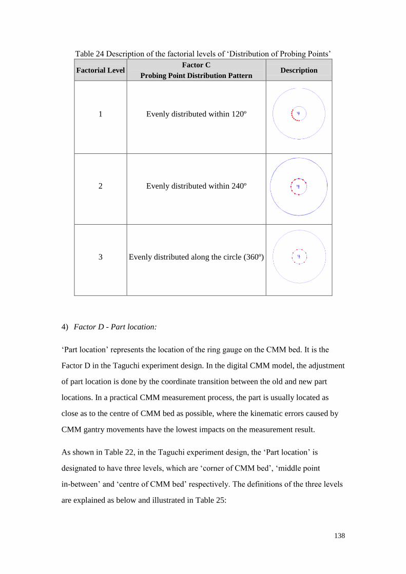
138

Table 24 Description of the factorial levels of ‘Distribution of Probing Points’

Factorial Level Factor C

Probing Point Distribution Pattern Description

1 Evenly distributed within 120º

2 Evenly distributed within 240º

3 Evenly distributed along the circle (360º)

4) Factor D - Part location:

‘Part location’ represents the location of the ring gauge on the CMM bed. It is the

Factor D in the Taguchi experiment design. In the digital CMM model, the adjustment

of part location is done by the coordinate transition between the old and new part

locations. In a practical CMM measurement process, the part is usually located as

close as to the centre of CMM bed as possible, where the kinematic errors caused by

CMM gantry movements have the lowest impacts on the measurement result.

As shown in Table 22, in the Taguchi experiment design, the ‘Part location’ is

designated to have three levels, which are ‘corner of CMM bed’, ‘middle point

in-between’ and ‘centre of CMM bed’ respectively. The definitions of the three levels

are explained as below and illustrated in Table 25:

139

Corner of CMM bed: the ‘corner of CMM bed’ is the origin (the (0,0,0) point) of

the CMM bed as shown in the first row of Table 25;

Centre of CMM bed: the ‘centre of CMM bed’ is the central point of the CMM

bed. The working volume of the CMM is mmmmmm 400500550 . Therefore

the coordinates of the ‘centre of CMM bed’ is (275, 250, 0). The location of the

‘centre of CMM bed’ is visualized in the digital CMM model as shown in the

third row of Table 25;

Middle point in-between: the ‘middle point in-between’ is the midpoint of the line

between the ‘corner of CMM bed’ and the ‘centre of CMM bed’. Therefore the

coordinates of the ‘middle point in-between’ is (137.5, 125, 0). The location of the

‘middle point in-between’ is shown in the second row of Table 25.

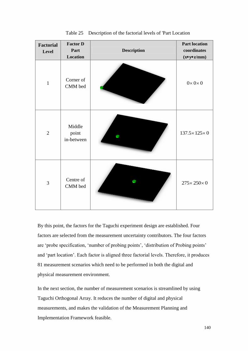
140

Table 25 Description of the factorial levels of 'Part Location

Factorial

Level

Factor D

Part

Location

Description

Part location

coordinates

(xyz/mm)

1 Corner of

CMM bed

000

2

Middle

point

in-between

01255.137

3 Centre of

CMM bed

0250275

By this point, the factors for the Taguchi experiment design are established. Four

factors are selected from the measurement uncertainty contributors. The four factors

are ‘probe specification, ‘number of probing points’, ‘distribution of Probing points’

and ‘part location’. Each factor is aligned three factorial levels. Therefore, it produces

81 measurement scenarios which need to be performed in both the digital and

physical measurement environment.

In the next section, the number of measurement scenarios is streamlined by using

Taguchi Orthogonal Array. It reduces the number of digital and physical

measurements, and makes the validation of the Measurement Planning and

Implementation Framework feasible.

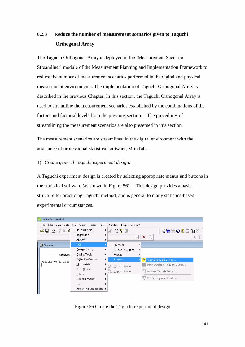
141

6.2.3 Reduce the number of measurement scenarios given to Taguchi

Orthogonal Array

The Taguchi Orthogonal Array is deployed in the ‘Measurement Scenario

Streamliner’ module of the Measurement Planning and Implementation Framework to

reduce the number of measurement scenarios performed in the digital and physical

measurement environments. The implementation of Taguchi Orthogonal Array is

described in the previous Chapter. In this section, the Taguchi Orthogonal Array is

used to streamline the measurement scenarios established by the combinations of the

factors and factorial levels from the previous section. The procedures of

streamlining the measurement scenarios are also presented in this section.

The measurement scenarios are streamlined in the digital environment with the

assistance of professional statistical software, MiniTab.

1) Create general Taguchi experiment design:

A Taguchi experiment design is created by selecting appropriate menus and buttons in

the statistical software (as shown in Figure 56). This design provides a basic

structure for practicing Taguchi method, and is general to many statistics-based

experimental circumstances.

Figure 56 Create the Taguchi experiment design

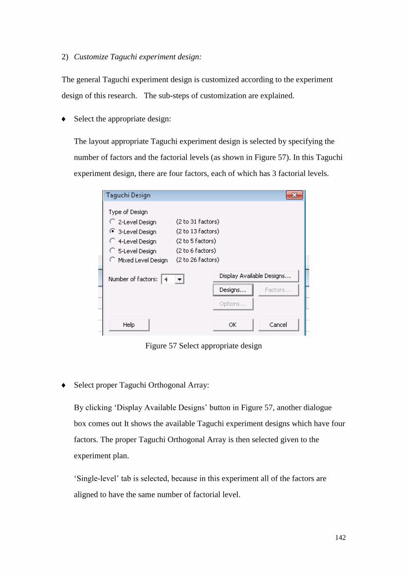
142

2) Customize Taguchi experiment design:

The general Taguchi experiment design is customized according to the experiment

design of this research. The sub-steps of customization are explained.

Select the appropriate design:

The layout appropriate Taguchi experiment design is selected by specifying the

number of factors and the factorial levels (as shown in Figure 57). In this Taguchi

experiment design, there are four factors, each of which has 3 factorial levels.

Figure 57 Select appropriate design

Select proper Taguchi Orthogonal Array:

By clicking ‘Display Available Designs’ button in Figure 57, another dialogue

box comes out It shows the available Taguchi experiment designs which have four

factors. The proper Taguchi Orthogonal Array is then selected given to the

experiment plan.

‘Single-level’ tab is selected, because in this experiment all of the factors are

aligned to have the same number of factorial level.

143

A table is listed as in Figure 58, summarizing the single-level Taguchi designs

available. The number following the "L" indicates the number of runs in the

design. The numbers in the table indicate the minimum and maximum number of

available factors for each design. Given to the requirements of this experiment

design, L9 (2-4) is selected. It indicates that the ring gauge measurements need to

run under nine measurement scenarios.

The experiment plan is a 4-factor and 3-factorial-level design, which originally

requires 81 experimental runs. By applying the Taguchi Orthogonal Array, the

number of experimental runs is reduced to 9.

Figure 58 Select proper Taguchi Orthogonal Array

Specify the number of trails for each run:

After specifying the number of runs, the number of trails for each run is selected.

Figure 59 is the dialogue box where the number of trails is selected. According to

the experiment plan, L27 (3-4) is selected. For each run, there are three trails to

perform. It indicates that the ring gauge measurements are performed three times

144

under each selected measurement scenario. Therefore, there are totally 27

measurements to perform.

Figure 59 Specify the number of runs of each measurement scenario

Align the factor names to the Taguchi experiment design:

According to the experiment plan, the names of measurement uncertainty

contributors are aligned to the Taguchi design factors through the dialogue box as

shown in Figure 60. The four measurement uncertainty contributors are ‘probe

specification’, ‘number of probing point’, ‘distribution of probing points’ and

‘part location’. Each of the factor has three factorial levels.

145

Figure 60 Align the factor names to the design

3) Streamline measurement scenarios:

By applying the Taguchi orthogonal array, the number of measurement scenarios is

reduced from 27 to 9. Table 26 concludes the measurement scenarios after

streamlining. The factors and the factorial levels appear equally in the selected

measurement scenarios, so the analysis can give a comprehensive result on the overall

experiment.

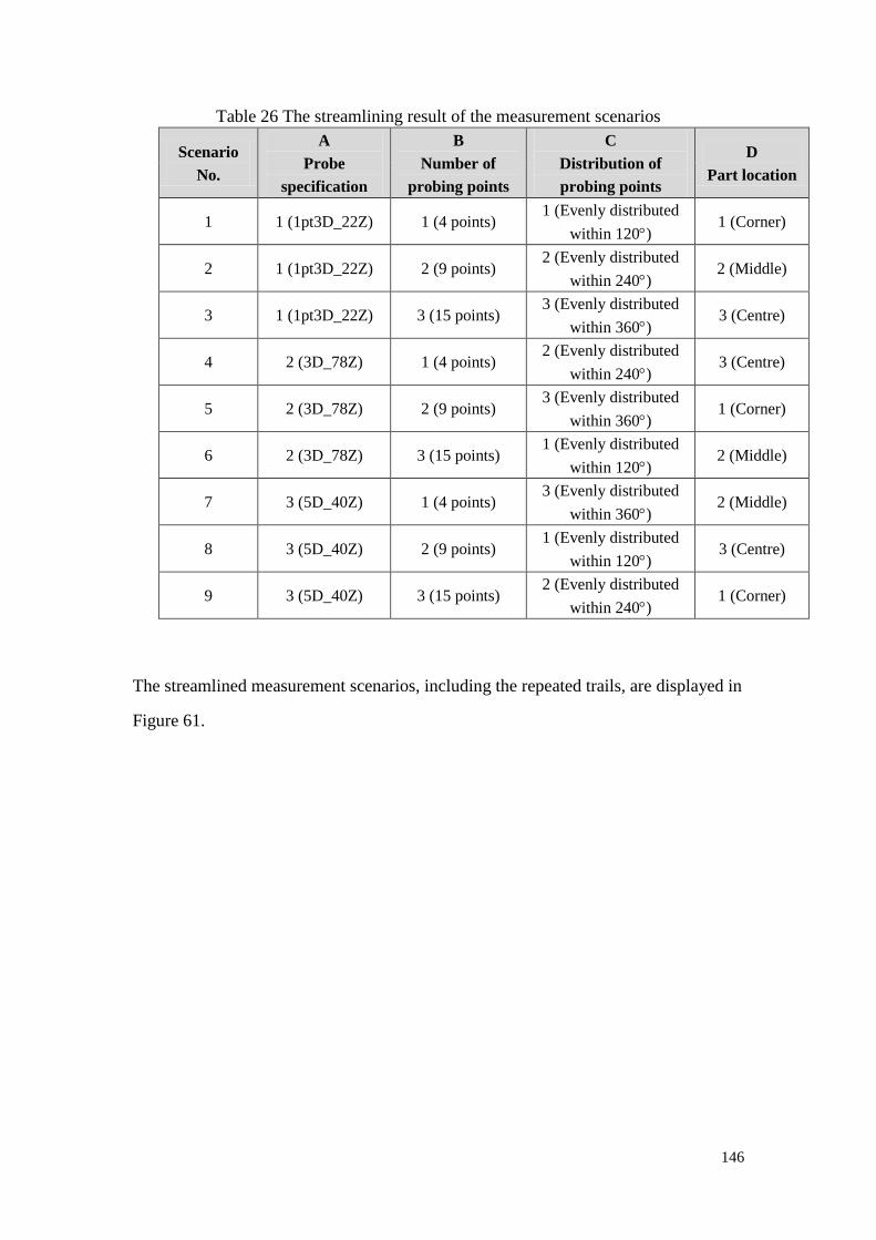
146

Table 26 The streamlining result of the measurement scenarios

Scenario

No.

A

Probe

specification

B

Number of

probing points

C

Distribution of

probing points

D

Part location

1 1 (1pt3D_22Z) 1 (4 points) 1 (Evenly distributed

within 120) 1 (Corner)

2 1 (1pt3D_22Z) 2 (9 points) 2 (Evenly distributed

within 240) 2 (Middle)

3 1 (1pt3D_22Z) 3 (15 points) 3 (Evenly distributed

within 360) 3 (Centre)

4 2 (3D_78Z) 1 (4 points) 2 (Evenly distributed

within 240) 3 (Centre)

5 2 (3D_78Z) 2 (9 points) 3 (Evenly distributed

within 360) 1 (Corner)

6 2 (3D_78Z) 3 (15 points) 1 (Evenly distributed

within 120) 2 (Middle)

7 3 (5D_40Z) 1 (4 points) 3 (Evenly distributed

within 360) 2 (Middle)

8 3 (5D_40Z) 2 (9 points) 1 (Evenly distributed

within 120) 3 (Centre)

9 3 (5D_40Z) 3 (15 points) 2 (Evenly distributed

within 240) 1 (Corner)

The streamlined measurement scenarios, including the repeated trails, are displayed in

Figure 61.

147

Figure 61 The streamlined measurement scenarios

4) Create data collection sheet:

At last, the streamlined measurement scenarios are collectively organized in the Excel

Table. The data collection sheet is created (as shown in Appendix C), which is used to

record the digital and physical measurement results.

6.2.4 The measurement process in the digital CMM model

The fundamentals of the digital CMM model have been introduced in the previous

chapters. The digital CMM model perceives the design and manufacturing

information from the part CAD model, and simulates the CMM measurement process

to predict task-specific measurement uncertainty. The digital CMM model provides

options allowing the end-user to customize the digital measurement given to the

conditions of the physical measurement. These options include diverse factors which

148

can potentially influence the CMM measurement process, e.g. temperature, CMM

machine specification, probe specification and probing strategy etc. These options

constrain the space of the CMM measurement uncertainty for the defined

measurement tasks. Then the digital CMM model performs the

simulation-by-constraints calculation to predict the task-specific measurement

uncertainty.

The digital measurement process in this section basically follows the above workflow,

but also is customized given to the special needs of the Framework validation. The

digital measurement process in this case is shown in Figure 62.

149

1) Import the CAD model into

digital CMM model

Create complete definition of

the ring gauge

Define measurement plan

Define measurement resources

2) Specify feature and

tolerances

3) Establish datum reference

frame

4) Characterize CMM machine

5) Define probe specification

6) Specify temperature

condition

7) Place the ring gauge on

CMM working volume

8) Select measured features

9) Define probing strategy

10) Calculate task-specific

measurement uncertainty using

simulate-by-constraints method

11) Collect simulation results

Figure 62 The measurement process in the digital CMM model

150

The individual steps of the digital measurement process are numbered in Figure 62.

The details of these individual steps are described as below:

1) Import the CAD model into digital CMM model:

The CAD model of the ring gauge is transformed into DMIS format file, and loaded

into the digital CMM model (as shown in Figure 63).

Figure 63 Import the CAD model of the ring gauge into the digital CMM model

2) Specify feature and tolerances:

The second step is to specify the tolerance characteristics of the measure feature.

Although the CAD-model of the ring gauge is created in the feature-based design

environment, this step is necessary. Because in the-state-of-the-art of computer-aided

151

inspection planning, the graphical entities that make up a solid model do not necessarily

correspond on a one-to-one basis with the measurement features of the part. It is still

necessary to create relationships between the graphical entities and the tolerance

features.

In this experiment, the tolerance characteristics are manually assigned to the

CAD-model of the ring gauge. As specified in the previous section, two tolerances are

assigned, which are diameter and cylindricity (as shown in Figure 64). The values of

the tolerances are also applied. The diameter of the inner hole is 10mm, of which

tolerance is 0.0009mm. The cylindricity tolerance of the inner hole is 0.0009mm.

Figure 64 Assign the tolerances to the ring gauge CAD model

152

At this point, the measured characteristics are assigned to the part. The remaining tasks

are to establish measurement datum, and to infer the measured characteristics with the

measurement datum.

3) Establish datum reference frame:

The method and concerns of establishing measurement datum are the same in both of

the digital CMM model and the physical measurement process. The datum reference

frame is established given to the nature of the ring gauge and the measurement tasks.

The top surface of the ring gauge serves as the primary datum feature, by measuring

which a flat plane is created. The surface of inner hole serves as the secondary datum

feature, by measuring which the central axis of the inner hole is created. The plane and

the central axis intersect at one point, which creates the datum point. Based on this

datum point, the datum reference frame is established.

In the digital CMM model, the top surface of the ring gauge is selected to be the

primary datum and denoted as DRF-A. The surface of the inner hole is selected to be

the secondary datum and denoted as DRF-B. On the computer screen, the DRF-B label

is dragged under the DRF-A label, and a completed datum reference frame is created as

shown in Figure 65.

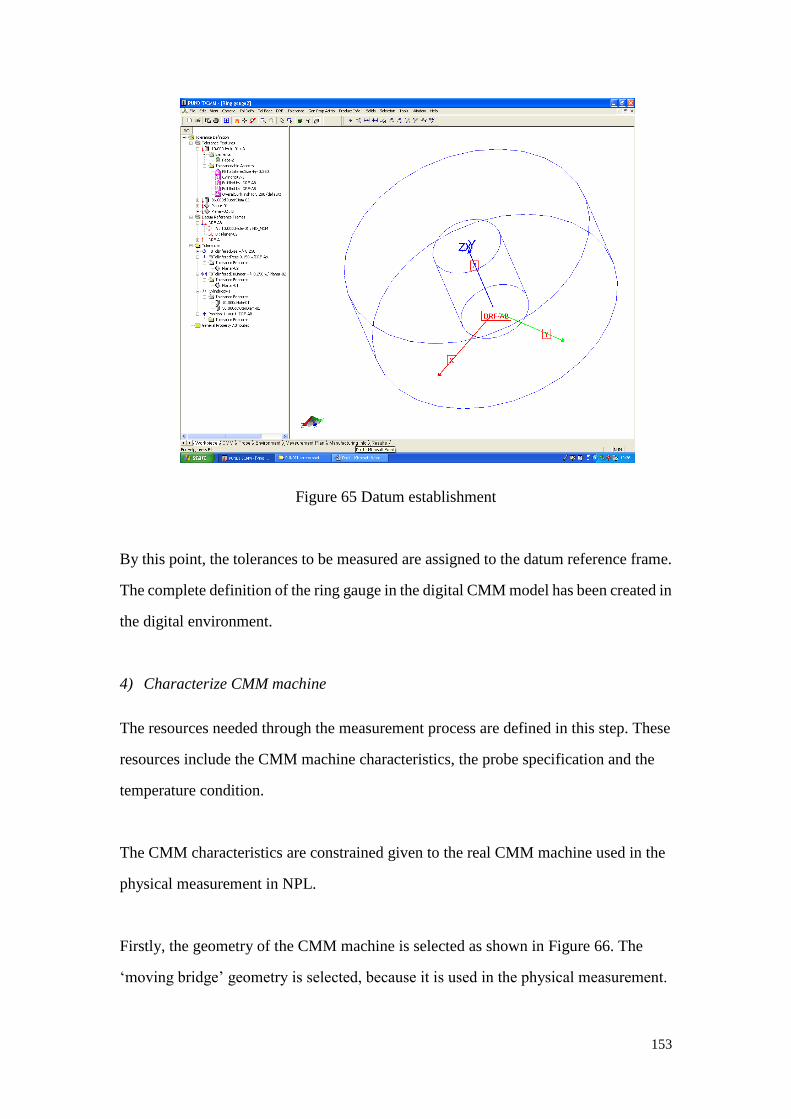
153

Figure 65 Datum establishment

By this point, the tolerances to be measured are assigned to the datum reference frame.

The complete definition of the ring gauge in the digital CMM model has been created in

the digital environment.

4) Characterize CMM machine

The resources needed through the measurement process are defined in this step. These

resources include the CMM machine characteristics, the probe specification and the

temperature condition.

The CMM characteristics are constrained given to the real CMM machine used in the

physical measurement in NPL.

Firstly, the geometry of the CMM machine is selected as shown in Figure 66. The

‘moving bridge’ geometry is selected, because it is used in the physical measurement.

154

Figure 66 Select the geometry of the CMM machine

Secondly, the working volume of the CMM machine is defined in the digital CMM

model (as shown in Figure 6768). Given to the CMM machine used in the physical

measurement, the working volume of the digital CMM machine is defined as 550mm x

500mm x 400mm.

Figure 6768 Define working volume of the CMM machine

155

Thirdly, the verification information of the CMM machine is loaded in the digital

CMM model (as shown Figure 69). The verification information requires the

specification of four categories of information inputs, which are ‘Error Model’, ‘Model

Data Source’, ‘Artefact Type’ and ‘Error of Indication’. The details and specific input

values to these modules are described below:

‘Error Model’: The ‘Error Model’ asks the end-user to specify the uncertainty

calculation method. The digital CMM model provides three uncertainty calculation

methods, which are ‘Perfect Machine’, ‘Simulation by Constraints’ and ‘Full

Parametric Specification’. Given the research aim, the Error Model is selected to be

‘Simulation by Constraints’.

‘Model Data Source’: The ‘Model Data Source’ module asks the end-user to

specify the verification standard based on which the CMM machine is tested. The

verification methods and results create the CMM performance data set as

mentioned in the previous sections. The CMM performance data set establishes the

constraints of the CMM performance in the digital environment. Then the digital

CMM model performs a simulation-by-constraints calculation to calculate

task-specific measurement uncertainty.

As shown in Figure 69, the digital CMM model provides three Model Data Sources,

which are ASME B89, ISO 10360 and the USAF calibration test. ASME B89

requests full linear accuracy test, of which result is not supplied with the CMM

machine in the physical measurement. USAF calibration is the verification standard

used by US Air Force, which is not accessible. Therefore, ISO 10360 is selected to

represent the CMM verification standard.

‘Artefact Type’ and ‘Position’: The ‘Artefact Type’ module and ‘Position’

module requests the end-user to specify the details during the full liner accuracy

test, including which type of calibrated artefact is used and how the calibrated

artefact is position on the CMM machine. ISO 10360, selected in the ‘Model Data

156

Source’, does not require the full liner accuracy test. Therefore, the two modules are

left blank (as shown in Figure 69).

Figure 69 Load the verification information in the digital CMM model

‘Error of Indication’: The ‘Error of Indication’ module asks the end-user to specify

the CMM verification result(s) given on the verification standard selected. In this

case, the CMM verification result is 1.3 + L/300 m, which is loaded in the digital

CMM model as shown in Figure 69.

5) Define probe specification:

The probe used to measure the ring gauge is defined in this step. Figure 70 shows the

dialogue box through which the probe specification is defined in the digital CMM

model.

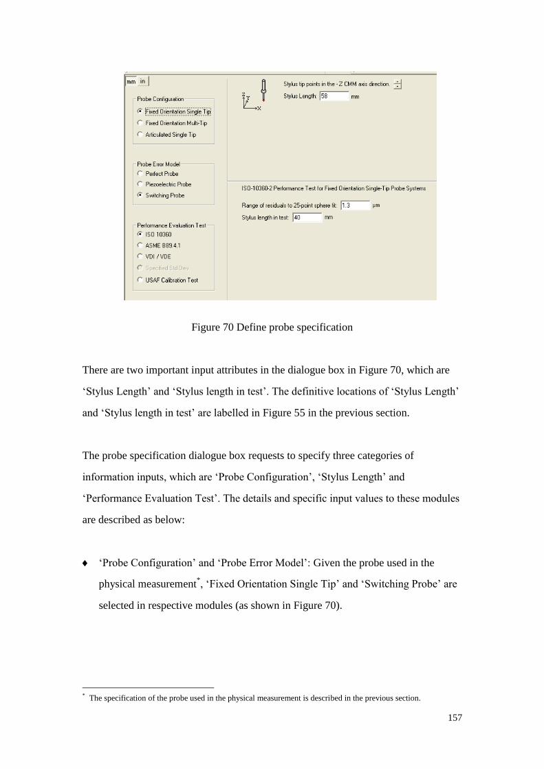
157

Figure 70 Define probe specification

There are two important input attributes in the dialogue box in Figure 70, which are

‘Stylus Length’ and ‘Stylus length in test’. The definitive locations of ‘Stylus Length’

and ‘Stylus length in test’ are labelled in Figure 55 in the previous section.

The probe specification dialogue box requests to specify three categories of

information inputs, which are ‘Probe Configuration’, ‘Stylus Length’ and

‘Performance Evaluation Test’. The details and specific input values to these modules

are described as below:

‘Probe Configuration’ and ‘Probe Error Model’: Given the probe used in the

physical measurement*, ‘Fixed Orientation Single Tip’ and ‘Switching Probe’ are

selected in respective modules (as shown in Figure 70).

* The specification of the probe used in the physical measurement is described in the previous section.

158

‘Stylus Length’ et al.: The ‘Stylus Length’ module in Figure 70 asks the end-user to

specify how the probe head is mounted in the CMM machine by designating the axis

direction that corresponds to the stylus tip pointing and stylus length.

In the Taguchi experiment design, the ‘Stylus Length’ is selected to be an

uncertainty contributor. Therefore, the input values of the ‘Stylus Length’ vary

between the measurement scenarios, the details of which will be presented in the

next section.

‘Performance Evaluation Test’ et al.: ‘Performance Evaluation Test’ and other

modules ask the end-user to specify the probe testing procedure and testing results.

The probes used in the physical measurements in NPL are tested accoording to the

ISO 10360 requirements, and hence the option ‘ISO 10360’ in the ‘Performance

Evaluation Test’ module is selected.

The rest of two attribute inputs, ‘Range of residuals to 25-point sphere fit’ and

‘Stylus length in test’ represent the probe testing results, which is selected to be an

uncertainty contributor in the Taguchi experiment design. The input values of these

attributes vary between the measurement scenarios. The details of their input values

are presented in the previous section.

6) Specify temperature condition:

The temperature condition during the measurement process is specified in this step.

Figure 71 shows the dialogue box where end-user can define the temperature condition

in the digital CMM model.

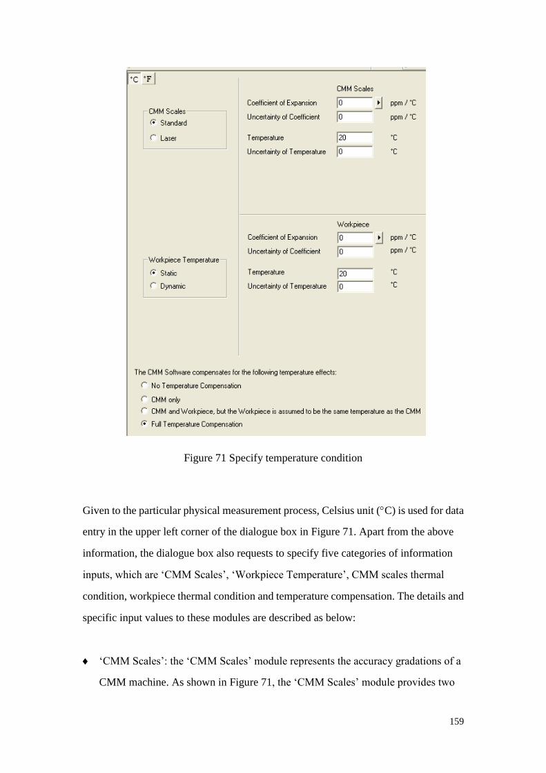
159

Figure 71 Specify temperature condition

Given to the particular physical measurement process, Celsius unit (C) is used for data

entry in the upper left corner of the dialogue box in Figure 71. Apart from the above

information, the dialogue box also requests to specify five categories of information

inputs, which are ‘CMM Scales’, ‘Workpiece Temperature’, CMM scales thermal

condition, workpiece thermal condition and temperature compensation. The details and

specific input values to these modules are described as below:

‘CMM Scales’: the ‘CMM Scales’ module represents the accuracy gradations of a

CMM machine. As shown in Figure 71, the ‘CMM Scales’ module provides two

160

options, ‘Standard’ and ‘Laser’. The majority of CMMs are equipped with

mechanical scales and optical reader heads that move along those scales to encode

the axis positions. A few CMMs, primarily, those designed to produce

measurements of extremely high accuracy are equipped with laser interferometer

scales. For the CMM used in the physical measurement of this research, ‘Standard’

CMM scale is selected.

‘Workpiece Temperature’: the ‘Workpiece Temperature’ module represents the

workpiece temperature changes over time. It provides two options, ‘Static’ and

‘Dynamic’. A ‘Static’ temperature model means that the temperature does not

change over the time, while a ‘Dynamic’ temperature model means that the

workpiece temperature may change with time. The physical measurements are

carried out in the finely-controlled laboratory environment, where the temperature

variation is very low. Therefore, in the digital CMM model, the ‘Static’ workpiece

temperature model is selected (as shown in Figure 71).

CMM Scales thermal condition: The attributes to define the CMM scales thermal

condition is on the upper right side in the dialogue box in Figure 71. It concerns the

thermal state of the CMM machine under the environment temperature change. The

physical measurements are carried out in the finely-controlled laboratory where the

temperature is maintained at 20C. Therefore, in the digital CMM model, the CMM

scales are established to work under the temperature of 20C, and the dynamic

thermal effects on the CMM machine are ignored (as shown in Figure 71).

Workpiece thermal condition: the attributes to define the workpiece thermal

condition is on the lower right side in the dialogue box in Figure 71. It concerns

the thermal condition of the workpiece under the environment temperature change.

The physical measurements are carried out in the finely-controlled laboratory

where the temperature is maintained at 20C. Therefore, in the digital CMM model,

the workpiece is established to work under the temperature of 20C, and the

dynamic thermal effects on the workpiece are ignored (as shown in Figure 71).

161

Temperature compensation: The temperature compensation module defines the

extent to which the CMM software attempts to compensate for thermal effects. Four

options are provided in the digital CMM model as shown in Figure 71. In the

physical measurement process, the CMM control software employs the ‘full

temperature compensation’ mode to manoeuvre the movements of CMM machine.

Consequently, in the digital measurement environment, the digital CMM model is

set to be ‘Full Temperature Compensation’ to follow the physical measurement

environment.

By this point, the resources needed for the measurement have been defined in the digital

CMM model. The next stage is to define the measurement plan as shown in Figure 62.

7) Place the ring gauge on CMM working volume:

In the digital CMM model, the measurement plan defines how the ring gauge is to be

measured: where it will be placed in the CMM working volume, which features will be

measured, how many data points are to be taken, where they are to be taken and with

what probe(s).

The first step of defining the measurement plan is to specify where to place the ring

gauge on the CMM working volume in the digital CMM model. The part location can

be defined through the dialogue box shown in Figure 72. The part can be moved by

entering the coordinates of the new location relative to the origin point which is at the

corner of the CMM’s working volume. This transformation process can be visualized

as shown in Figure 73.

162

Figure 72 Place the part on CMM working volume

Figure 73 Transform the part location

The part placement is selected to be an uncertainty contributor in the Taguchi

experiment design. The input values of these attributes vary between the measurement

scenarios. The details of their input values are presented in the previous section.

8) Select measured features:

163

In this step, the features to be measured are edited, so that the digital definitions of the

measurement tasks and operations can truly reflect the measurements needed in the

digital CMM mode. A ‘Measurement Definition’ tree is generated as shown in Figure

74. The Measure Features folder is populated to list the key features of the ring gauge.

For each Measure Feature there is an Elements sub-folder, a Datum Reference Frame

sub-folder and a Tolerances sub-folder. Each Measure Feature also has a Measure Task

Group folder.

Figure 74 Select measured features

As shown in Figure 74, the ring gauge has four features, which are the inner circle

(denoted as 10.000dHole-01M:A in Figure 74), the outer circle (denoted as

36.0000dOuter Diam-02M in Figure 74), the top surface (denoted as Planar-01M in

164

Figure 74) and the bottom surface (denoted as Plananr-02M:B in Figure 74). The inner

circle is the feature to be measured, so the folder of ‘10.000dHole-01M:A’ is expanded.

The ‘10.000dHole-01M:A’ folder has four sub-folders, which contains the key

information of measuring the inner circle of the ring gauge. The four sub-holders are

‘Elements’, ‘Datum Reference Frames’, ‘Tolerance’ and ‘Measure Task Group’. The

details of these four groups are described as below:

Elements: The ‘Elements’ sub-folder shows the surfaces which compose the inner

circle of the ring gauge. This sub-folder allows the end-user to define the measured

features by directly clicking the surfaces of the part CAD model.

Datum Reference Frames: The ‘Datum Reference Frames’ sub-folder shows the

measurement datum to which the measure feature is referenced. As defined in the

previous step, the datum for measuring the inner circle is composed by the

intersection of the central axis of the inner circle and the top surface of the ring

gauge, which are respectively denoted as ‘A’ and ‘B’ in the ‘Measurement

Definition’ tree in Figure 74.

Tolerance: The ‘Tolerance’ sub-folder shows the tolerances to be measured for the

feature. As shown in Figure 74, there are two tolerances to be measured on the inner

circle of the ring gauge, which are diameter and cylindricity.

Measure Task Group: The ‘Measure Task Group’ sub-folder shows the probing

strategy for measuring the feature. The details of defining the probing strategy,

which supplies the content of the ‘Measure Task Group’ sub-folder, are presented

in the next step.

9) Define probing strategy:

The details of the probing strategy are defined in this step. The number and placement of

measurement points for each feature are designated in the digital CMM model.

165

Figure 75 shows the dialogue box through which the probing strategy is aligned to the

inner circle of the ring gauge. For the geometric nature of the inner circle, the probing

strategy is defined through three attributes, which are ‘Points per Level’, ‘Number of

Levels’ and ‘Patter Type’. The values of the three attributes are manually inputted in

the digital CMM model to generate a complete probing strategy.

Figure 75 Probing strategy dialogue box

The result of arranging the probing strategy is visualized in the widow of the digital

CMM model. Figure 76 shows one of the probing strategies defined for measuring the

inner circle of the ring gauge. In this case, the ‘‘Points per Level’, ‘Number of Levels’

are set to be 20 and 5 respectively, meaning the sampling point distribution is 20 points

per level, and 5 levels. And the point distribution pattern is ‘Rectangular’.

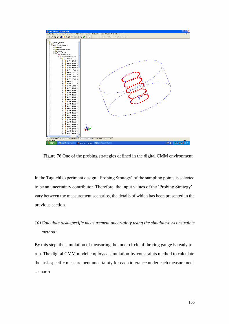
166

Figure 76 One of the probing strategies defined in the digital CMM environment

In the Taguchi experiment design, ‘Probing Strategy’ of the sampling points is selected

to be an uncertainty contributor. Therefore, the input values of the ‘Probing Strategy’

vary between the measurement scenarios, the details of which has been presented in the

previous section.

10) Calculate task-specific measurement uncertainty using the simulate-by-constraints

method:

By this step, the simulation of measuring the inner circle of the ring gauge is ready to

run. The digital CMM model employs a simulation-by-constraints method to calculate

the task-specific measurement uncertainty for each tolerance under each measurement

scenario.

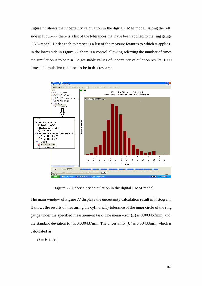
167

Figure 77 shows the uncertainty calculation in the digital CMM model. Along the left

side in Figure 77 there is a list of the tolerances that have been applied to the ring gauge

CAD-model. Under each tolerance is a list of the measure features to which it applies.

In the lower side in Figure 77, there is a control allowing selecting the number of times

the simulation is to be run. To get stable values of uncertainty calculation results, 1000

times of simulation run is set to be in this research.

Figure 77 Uncertainty calculation in the digital CMM model

The main window of Figure 77 displays the uncertainty calculation result in histogram.

It shows the results of measuring the cylindricity tolerance of the inner circle of the ring

gauge under the specified measurement task. The mean error (E) is 0.003453mm, and

the standard deviation () is 0.000437mm. The uncertainty (U) is 0.00433mm, which is

calculated as

2 EU.

168

6.2.5 Collect simulation results

The task-specific uncertainties calculated by the digital CMM model are recorded and

kept in the Excel table(s) for further analysis.

By this point, the task-specific measurement uncertainties are generated in the digital

CMM model based on the selected measurement scenarios. The input values of the

digital CMM model are decided given to the resources availability of the physical

measurements, and the measurement scenarios defined by the ‘Measurement Scenario

Streamliner’ module in the Measurement Planning and Implementation Framework.

The data collection from the digital measurement process is presented in the next

section.

6.3 Digital measurement results and Taguchi experimental analysis

6.3.1 Digital measurement results

The digital measurements are carried out as defined by the experiment design. The

measurement results are collected and presented in Table 27.

169

Table 27 Data collection of digital measurement results

Run

No.

Measurement scenarios Diameter result (m) Cylindricity result (m)

Probe

specification

Number of

probing

points

Distribution of

probing points

Part

location

Mean

error

Standard

deviation

Uncertainty Mean

error

Standard

deviation

Uncertainty

1 1pt3D_22Z 4 120 Corner 12.768 4.387 21.542 9.890 1.980 13.850

2 1pt3D_22Z 4 120 Corner 12.707 4.248 21.203 9.880 1.955 13.790

3 1pt3D_22Z 4 120 Corner 12.457 4.155 20.767 9.990 1.956 13.902

4 1pt3D_22Z 9 240 Middle 7.967 3.824 15.615 7.263 0.541 8.345

5 1pt3D_22Z 9 240 Middle 8.011 3.993 15.997 7.329 0.589 8.507

6 1pt3D_22Z 9 240 Middle 8.026 3.956 15.938 7.358 0.628 8.614

7 1pt3D_22Z 15 360 Centre 6.045 3.913 13.871 2.887 0.216 3.319

8 1pt3D_22Z 15 360 Centre 6.013 3.673 13.359 2.843 0.164 3.171

9 1pt3D_22Z 15 360 Centre 6.148 3.912 13.972 2.853 0.181 3.215

10 3D_78Z 4 240 Centre 4.157 1.655 7.467 2.812 0.439 3.690

11 3D_78Z 4 240 Centre 4.134 1.654 7.442 2.809 0.459 3.727

12 3D_78Z 4 240 Centre 4.134 1.654 7.442 2.788 0.447 3.682

13 3D_78Z 9 360 Corner 4.980 1.674 8.328 2.732 0.472 3.676

14 3D_78Z 9 360 Corner 4.966 1.647 8.260 2.726 0.466 3.658

15 3D_78Z 9 360 Corner 4.960 1.593 8.146 2.730 0.467 3.664

16 3D_78Z 15 120 Middle 6.487 1.868 10.223 2.487 1.440 5.367

17 3D_78Z 15 120 Middle 6.419 1.867 10.153 2.486 1.430 5.346

18 3D_78Z 15 120 Middle 6.431 1.856 10.143 2.488 1.470 5.428

19 5D_40Z 4 360 Middle 3.662 1.653 6.968 1.576 0.535 2.646

20 5D_40Z 4 360 Middle 3.576 1.560 6.696 1.564 0.536 2.636

21 5D_40Z 4 360 Middle 3.562 1.627 6.816 1.615 0.579 2.773

170

22 5D_40Z 9 120 Centre 5.518 1.678 8.874 3.570 0.840 5.250

23 5D_40Z 9 120 Centre 5.550 1.549 8.648 3.570 0.840 5.250

24 5D_40Z 9 120 Centre 5.556 1.633 8.822 3.570 0.940 5.450

25 5D_40Z 15 240 Corner 3.981 1.430 6.841 3.077 0.544 4.165

26 5D_40Z 15 240 Corner 3.899 1.480 6.859 3.087 0.554 4.195

27 5D_40Z 15 240 Corner 3.800 1.420 6.640 3.076 0.546 4.168

171

6.3.2 Taguchi experimental analysis of digital measurement results

The main effects plots of the means and S/N ratios are generated versus the control

factors. The linear model results for S/N ratios and means are displayed with respects

to diameter measurements and cylindricity measurements in the digital CMM model.

1) Diameter analysis result

The Taguchi analysis results of diameter measurements in digital environment are

summarized in Table 28 and Table 30. Table 28 shows the response table and main

effects plot for the means, and Figure 71 shows the response table and main effects

plot for the S/N ratios. The interpretations of Table 28 and in Figure 71 are presented

in the following paragraphs.

A. The effects of the control factors on the mean values

Table 28 reveals the effects of the selected control factors on the mean values of

measurement uncertainty by measuring the diameter of the ring gauge in the digital

CMM model. The numbers in Table 28 quantitatively represent the effects on the

mean value of measurement uncertainty for each level of each control factor. Based

on these numbers, the ‘Main Effects Plot for Mean’ is constructed. The Plot visually

shows how the selected control factors influence the measurement results.

172

Table 28 Analysis of the means for diameter measurements in digital environment

Response Table for Means

Factorial

Level

Control Factors

Probe

specification

Number of

probing points

Distribution of

probing points

Part

location

1 16.918 11.816 13.375 9.989

2 8.623 10.959 10.027 12.065

3 7.463 10.229 9.602 10.950

Delta 9.456 1.587 3.773 2.077

Rank 1 4 2 3

Main Effects Plot for Means

5D_40Z3D_78Z1pt3D_22Z

16

14

12

10

8

1594

360240120

16

14

12

10

8

CornerMiddleCentre

Probe specification

Me

an

of

Me

an

s

Number of probing points

Distributrion of probing points Part location

Main Effects Plot for MeansData Means

Key

words: Digital measurement, diameter, mean.

From the ‘Main Effects Plot for Mean’ in Table 28, two tendencies are observed

directly: a) the diameter measurement is influenced by the selected measurement

uncertainty contributors; b) Different measurement uncertainty contributors have

different effects on the diameter measurement results. These two points are described

and discussed in more detail in the following paragraphs.

a) The diameter measurement is influenced by the selected measurement uncertainty

contributors. The mean value of the diameter measurement uncertainties,

173

determined from the digital measurements, changes over the changes of ‘probe

specification’, ‘number of probing points’, ‘distribution of probing points’ and

‘part location’. Several points are made by examining the ‘Main Effects Plot for

Mean’ against the control factors:

Probe specification: The mean value of measurement uncertainty decreases

significantly when it is switched to better CMM probe. In particularly, the

measurement uncertainty reduces significantly between Probe 1pt3D_22Z and

3D_78Z. The Taguchi analysis result of the factor effect conforms to common

understandings on CMM measurement.

Number of probing points: The mean value of measurement uncertainty

decreases when the number of probing points increases. The measurement

results are improved by probing more points on the feature. The Taguchi

analysis result of the factor effect conforms to common understandings on

CMM measurement.

Distribution of probing points: The mean value of measurement uncertainty

decreases significantly, when the probing points are distributed more evenly

around the circle. In particularly, the measurement uncertainty reduces

significantly between 120-distribution and 240-distribution. The Taguchi

analysis result of the factor effect conforms to common understandings on

CMM measurement.

Part location: The mean value of measurement uncertainty changes over the

change of part location. As the part is moved from the corner of the CMM bed

to the centre, the Plot shows an overall decrease of the measurement

uncertainty. However, on the middle point of the centre-corner line, the

measurement uncertainty unexpectedly goes higher than the one on the corner

point. The Taguchi analysis result of the factor effect conforms to common

understandings on CMM measurement, except the one at the ‘middle’ point. It

is possibly accounted by the nature of ‘simulation-by-constraints’ method,

which popularizes a large amount of digital CMMs, and consequently is lack

of the sensitivity to the part location adjustment on CMM bed.

174

b) Different measurement uncertainty contributors have different effects on the

diameter measurement results. The range of the measurement uncertainty change

varies between the selected control factors. The ranks of the factor effects are

assigned based on the Delta statistics calculation*, which compare the relative

magnitude of effects. The Delta values of the control factors are presented in the

‘Response Table for Means’ in Table 28.

From Table 28, it can be seen that ‘probe specification’ has the greatest effect on

the mean value of measurement uncertainty. ‘Distribution of probing points’ has

the second greatest effect, followed by ‘part location’ and ‘number of probing

points’. This Taguchi analysis results suggest that, the most effective way to

minimize the measurement uncertainty is to switch to a better CMM probe, and

the second effective way is to evenly distribute probing points. Positioning the

part in the centre of CMM bed is fairly effective, but not as effective as the former

two options. Increasing the density of probing points has least effective impact on

CMM measurement result.

The rank drawn from the digital measurement environment is fairly close to the

rules-of-thumb in physical measurement. The rank of the control factor effects is

discussed in Table 29.

* The Delta statistic is the highest minus the lowest average for each factor. Rank 1 assigns to the

highest Delta value, rank 2 assigns to the second highest, and so on. Use the level averages in

the response tables to determine which level of each factor provides the best result.

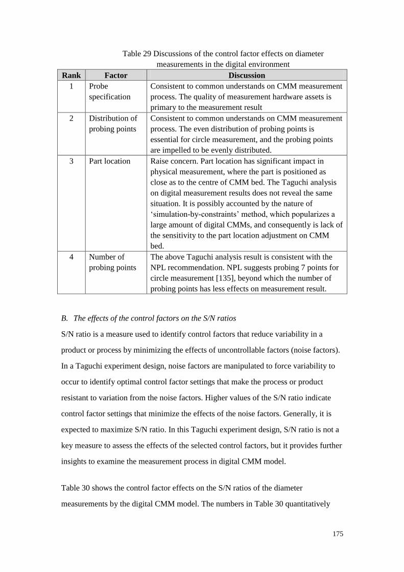
175

Table 29 Discussions of the control factor effects on diameter

measurements in the digital environment

Rank Factor Discussion

1 Probe

specification

Consistent to common understands on CMM measurement

process. The quality of measurement hardware assets is

primary to the measurement result

2 Distribution of

probing points

Consistent to common understands on CMM measurement

process. The even distribution of probing points is

essential for circle measurement, and the probing points

are impelled to be evenly distributed.

3 Part location Raise concern. Part location has significant impact in

physical measurement, where the part is positioned as

close as to the centre of CMM bed. The Taguchi analysis

on digital measurement results does not reveal the same

situation. It is possibly accounted by the nature of

‘simulation-by-constraints’ method, which popularizes a

large amount of digital CMMs, and consequently is lack of

the sensitivity to the part location adjustment on CMM

bed.

4 Number of

probing points

The above Taguchi analysis result is consistent with the

NPL recommendation. NPL suggests probing 7 points for

circle measurement [135], beyond which the number of

probing points has less effects on measurement result.

B. The effects of the control factors on the S/N ratios

S/N ratio is a measure used to identify control factors that reduce variability in a

product or process by minimizing the effects of uncontrollable factors (noise factors).

In a Taguchi experiment design, noise factors are manipulated to force variability to

occur to identify optimal control factor settings that make the process or product

resistant to variation from the noise factors. Higher values of the S/N ratio indicate

control factor settings that minimize the effects of the noise factors. Generally, it is

expected to maximize S/N ratio. In this Taguchi experiment design, S/N ratio is not a

key measure to assess the effects of the selected control factors, but it provides further

insights to examine the measurement process in digital CMM model.

Table 30 shows the control factor effects on the S/N ratios of the diameter

measurements by the digital CMM model. The numbers in Table 30 quantitatively

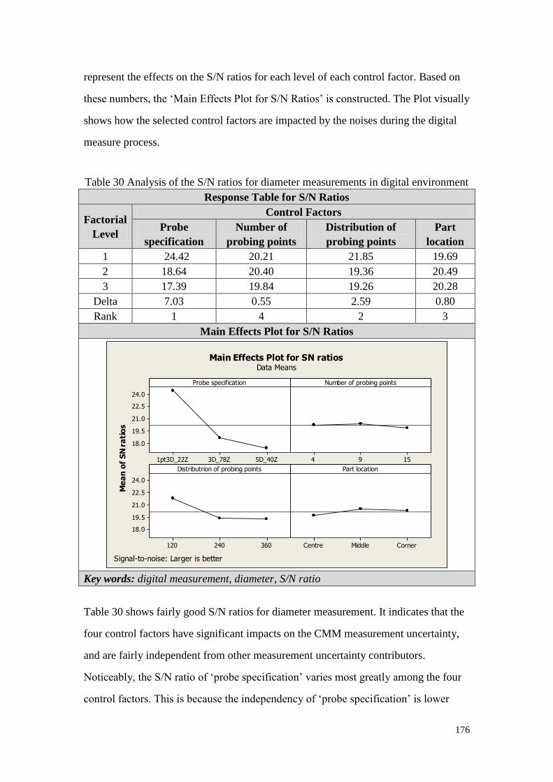
176

represent the effects on the S/N ratios for each level of each control factor. Based on

these numbers, the ‘Main Effects Plot for S/N Ratios’ is constructed. The Plot visually

shows how the selected control factors are impacted by the noises during the digital

measure process.

Table 30 Analysis of the S/N ratios for diameter measurements in digital environment

Response Table for S/N Ratios

Factorial

Level

Control Factors

Probe

specification

Number of

probing points

Distribution of

probing points

Part

location

1 24.42 20.21 21.85 19.69

2 18.64 20.40 19.36 20.49

3 17.39 19.84 19.26 20.28

Delta 7.03 0.55 2.59 0.80

Rank 1 4 2 3

Main Effects Plot for S/N Ratios

5D_40Z3D_78Z1pt3D_22Z

24.0

22.5

21.0

19.5

18.0

1594

360240120

24.0

22.5

21.0

19.5

18.0

CornerMiddleCentre

Probe specification

Me

an

of

SN

ra

tio

s

Number of probing points

Distributrion of probing points Part location

Main Effects Plot for SN ratiosData Means

Signal-to-noise: Larger is better

Key words: digital measurement, diameter, S/N ratio

Table 30 shows fairly good S/N ratios for diameter measurement. It indicates that the

four control factors have significant impacts on the CMM measurement uncertainty,

and are fairly independent from other measurement uncertainty contributors.

Noticeably, the S/N ratio of ‘probe specification’ varies most greatly among the four

control factors. This is because the independency of ‘probe specification’ is lower

177

than the other control factors. The ‘probe specification’ is composed by three

components, ‘stylus length in test’, ‘stylus tip point in the - z CMM axis direction’

and ‘range of residuals to 25-point sphere fit’, which possibly contribute more noises

over the measurement process. The digital analysis on S/N ratio conforms to the

physical measurement reality.

To conclude, the above Taguchi analysis has produced reasonable results in predicting

the effects of the control factors on measurement uncertainty of the diameter

measurements in a digital environment. Although the effect of ‘part location’ does not

completely conform to the rule-of-thumb in physical measurements, it can be

explained by the natural blemish of the simulation-by-constraints method employed in

the digital CMM model. The simulation-by-constraints method popularizes large

amount of virtual CMMs, and ignores the characteristics of individual CMM

machines. This limits the CMM digital model to sense the part location adjustments

on individual CMM machine. Consequently, it leads to the defect in Taguchi analysis

result of predicting the ‘part position’ effect on measurement uncertainty.

2) Cylindricity analysis result

The Taguchi analysis results of cylindricity measurements in the digital environment

are summarized in Table 31 and Table 33. Table 31 shows the response table and

main effects plot for the means, and Table 33 shows the response table and main

effects plot for the S/N ratios. The explanations of Table 31 and Table 33 are

presented in the following paragraphs.

A. The effects of the control factors on the mean values

Table 31 reveals the effects of the selected control factors on the mean values of

measurement uncertainty by measuring the cylindricity of the ring gauge in the digital

CMM model. The effects of the control factors observed from cylindricity

measurement are similar to the ones from diameter measurement.

178

Two tendencies are noted: a) The cylindricity measurement is influenced by the

selected measurement uncertainty contributors; b) Different measurement uncertainty

contributors have different effects on the cylindricity measurement results. These two

points are described and discussed in more detail in the following paragraphs.

Table 31 Analysis of the means for the cylindricity measurements in the digital

environment

Response Table for Means

Factorial

Level

Control Factors

Probe

specification

Number of

probing points

Distribution of

probing points

Part

location

1 6.699 4.769 5.326 3.078

2 2.673 4.539 4.400 5.243

3 2.745 2.809 2.392 3.796

Delta 4.026 1.960 2.934 2.165

Rank 1 4 2 3

Main Effects Plot for Means

5D_40Z3D_78Z1pt3D_22Z

9.0

7.5

6.0

4.5

3.0

1594

360240120

9.0

7.5

6.0

4.5

3.0

CornerMiddleCentre

Probe specification

Me

an

of

Me

an

s

Number of probing points

Distributrion of probing points Part location

Main Effects Plot for MeansData Means

Key words: digital measurement, cylindricity, mean

a) The cylindricity measurement is influenced by the selected measurement

uncertainty contributors. The mean value of the cylindricity measurement

uncertainties, determined from the digital measurements, changes over the

179

changes of ‘probe specification’, ‘number of probing points’, ‘distribution of

probing points’ and ‘part location’. Several points are made by examining the

‘Main Effects Plot for Mean’ against the control factors.

Probe specification: The mean value of measurement uncertainty decreases

significantly when it is switched to better CMM probe. In particularly, the

measurement uncertainty reduces significantly between Probe 1pt3D_22Z and

3D_78Z. This digital analysis result conforms to common understandings on

CMM measurement.

Number of probing points: The mean value of measurement uncertainty

decreases when the number of probing points increases. The measurement

results are improved by probing more points on the feature. This digital

analysis result conforms to common understandings on CMM measurement.

Distribution of probing points: The mean value of measurement uncertainty

decreases fairly significantly, when the probing points are distributed more

evenly around the circle. This digital analysis result conforms to common

understandings on CMM measurement.

Part location: The mean value of measurement uncertainty changes over the

change of part location. As the part is moved from the corner of the CMM bed

to the centre, the Plot shows an overall decrease of the measurement

uncertainty. However, on the middle point of the centre-corner line, the

measurement uncertainty unexpectedly goes higher than the one on the corner

point. This digital analysis result generally conforms to common

understandings on CMM measurement, except the one at the ‘middle’ point. It

is possibly accounted by the nature of ‘simulation-by-constraints’ method,

which popularizes a large amount of digital CMMs, and consequently is lack

of the sensitivity to the part location adjustment on CMM bed.

b) Different measurement uncertainty contributors have different effects on the

cylindricity measurement results. The range of the measurement uncertainty

change varies between the selected control factors.

180

From Table 31, it can be seen that ‘probe specification’ has the greatest effect on

the mean value of measurement uncertainty. ‘Distribution of probing points’ has

the second greatest effect, followed by ‘part location’ and ‘number of probing

points’. This Taguchi analysis results suggest that, the most effective way to

minimize the measurement uncertainty is to switch to a better CMM probe, and

the second effective way is to evenly distribute probing points. Positioning the

part in the centre of CMM bed is fairly effective, but not as effective as the former

two options. Increasing the density of probing points has the least effective impact

on the CMM measurement result.

The rank drawn from the digital measurement environment is fairly close to the

rules-of-thumb in physical measurement. The discussions of the control factor

effects are summarized in Table 32.

181

Table 32 Discussions of the control factor effects on cylindricity measurements

Rank Factor Discussion

1 Probe

specification

Consistent with the rule-of-thumb in physical measurement.

The quality of measurement hardware assets is primary to

the measurement result

2 Distribution

of probing

points

Consistent with the rule-of-thumb in physical measurement.

The even distribution of probing points is essential for circle

measurement, and the probing points are impelled to be

evenly distributed.

3 Part location Raise concern. Part location has significant impact in

physical measurement, where the part is positioned as close

as to the centre of CMM bed. The Taguchi analysis on

digital measurement results does not reveal the same

situation. It is possibly accounted by the nature of

‘simulation-by-constraints’ method, which popularizes a

large amount of digital CMMs, and consequently is lack of

the sensitivity to the part location adjustment on CMM bed.

4 Number of

probing points

The Taguchi analysis result is consistent with the NPL

recommendation. NPL suggests probing 7 points for circle

measurement [135], beyond which the number of probing

points has less effects on measurement result. The above

Taguchi analysis result is consistent with the NPL

recommendation.

B. The effects of the control factors on the S/N ratios

Table 33 shows the control factor effects on the S/N ratios of the cylindricity

measurements by the digital CMM model.

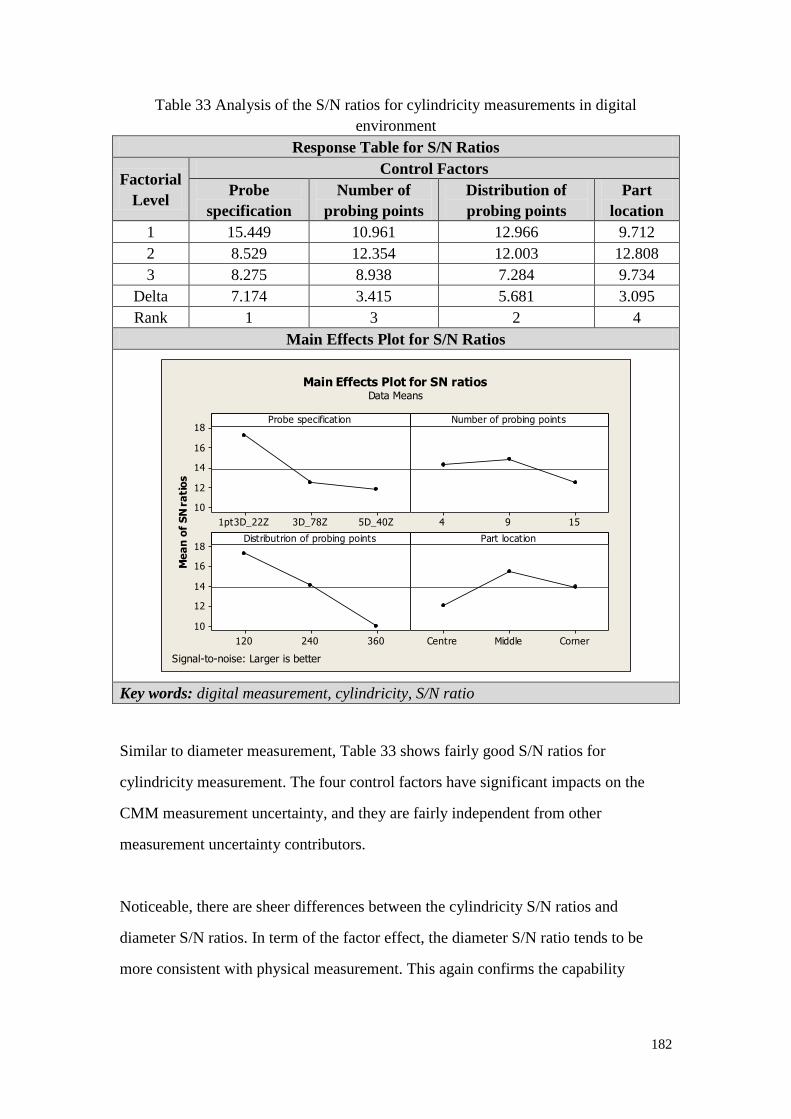
182

Table 33 Analysis of the S/N ratios for cylindricity measurements in digital

environment

Response Table for S/N Ratios

Factorial

Level

Control Factors

Probe

specification

Number of

probing points

Distribution of

probing points

Part

location

1 15.449 10.961 12.966 9.712

2 8.529 12.354 12.003 12.808

3 8.275 8.938 7.284 9.734

Delta 7.174 3.415 5.681 3.095

Rank 1 3 2 4

Main Effects Plot for S/N Ratios

5D_40Z3D_78Z1pt3D_22Z

18

16

14

12

10

1594

360240120

18

16

14

12

10

CornerMiddleCentre

Probe specification

Me

an

of

SN

ra

tio

s

Number of probing points

Distributrion of probing points Part location

Main Effects Plot for SN ratiosData Means

Signal-to-noise: Larger is better

Key words: digital measurement, cylindricity, S/N ratio

Similar to diameter measurement, Table 33 shows fairly good S/N ratios for

cylindricity measurement. The four control factors have significant impacts on the

CMM measurement uncertainty, and they are fairly independent from other

measurement uncertainty contributors.

Noticeable, there are sheer differences between the cylindricity S/N ratios and

diameter S/N ratios. In term of the factor effect, the diameter S/N ratio tends to be

more consistent with physical measurement. This again confirms the capability

183

variance of the digital CMM model, which performs superior in length measurement

than in form measurement in uncertainty calculations.

Table 34 lists The ‘Main Effects Plot(s) for SN ratios’ for both of diameter and

cylindricity measurements, by comparing which several differences are realized:

a) The S/N ratio of diameter measurement is generally higher than the one of

cylindricity measurement. In the digital measurement environment, signal from

diameter measurement is generally stronger than from cylindricity measurement.

This confirms that it is easier to estimate task-specific measurement uncertainty

for length measurement than for form measurements by digital measurement

models;

b) For a single control factor, the S/N ratios in cylindricity measurements generally

have greater variations than the ones in diameter measurements. Cylindricity

uncertainty estimation is affected by more noises than diameter uncertainty

estimation. Again, this indicates that uncertainty estimation for form tolerance is

more complicated than for length tolerance. The algorithm for calculating

cylindricity measurement uncertainty requires more efforts to determine the

complete mathematical description of the CMM task-specific measurement

process. On the other hand, this Taguchi analysis result reflects that the digital

CMM is not as capable in predicting form measurement uncertainty compared

with length measurement uncertainty;

c) The factor effects on S/N ratios in cylindricity measurement and diameter

measurements are different. Fox example, in cylindricity measurements the

‘distribution of the probing points’ has the greatest, while in diameter

measurements, the ‘probe specification’ has the greatest effect. In term of the

factor effect, the diameter S/N ratio tends to be more consistent with physical

measurement. This again confirms the capability variance of the digital CMM

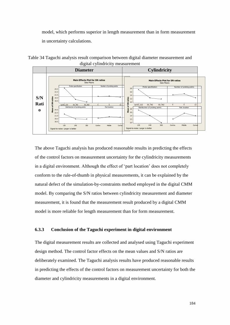
184

model, which performs superior in length measurement than in form measurement

in uncertainty calculations.

Table 34 Taguchi analysis result comparison between digital diameter measurement and

digital cylindricity measurement

Diameter Cylindricity

S/N

Rati

o

5D_40Z3D_78Z1pt3D_22Z

24.0

22.5

21.0

19.5

18.0

1594

360240120

24.0

22.5

21.0

19.5

18.0

CornerMiddleCentre

Probe specification

Me

an

of

SN

ra

tio

s

Number of probing points

Distributrion of probing points Part location

Main Effects Plot for SN ratiosData Means

Signal-to-noise: Larger is better

5D_40Z3D_78Z1pt3D_22Z

18

16

14

12

10

1594

360240120

18

16

14

12

10

CornerMiddleCentre

Probe specification

Me

an

of

SN

ra

tio

s

Number of probing points

Distributrion of probing points Part location

Main Effects Plot for SN ratiosData Means

Signal-to-noise: Larger is better

The above Taguchi analysis has produced reasonable results in predicting the effects

of the control factors on measurement uncertainty for the cylindricity measurements

in a digital environment. Although the effect of ‘part location’ does not completely

conform to the rule-of-thumb in physical measurements, it can be explained by the

natural defect of the simulation-by-constraints method employed in the digital CMM

model. By comparing the S/N ratios between cylindricity measurement and diameter

measurement, it is found that the measurement result produced by a digital CMM

model is more reliable for length measurement than for form measurement.

6.3.3 Conclusion of the Taguchi experiment in digital environment

The digital measurement results are collected and analysed using Taguchi experiment

design method. The control factor effects on the mean values and S/N ratios are

deliberately examined. The Taguchi analysis results have produced reasonable results

in predicting the effects of the control factors on measurement uncertainty for both the

diameter and cylindricity measurements in a digital environment.

185

The defects in the Taguchi analysis results can be explained. Two major defects are:

a) The simulation-by-constraints method, deployed in the digital CMM model, is

not capable of sensing the individual characteristics of a CMM machine. It limits

the CMM digital model to sense the part adjustments on individual CMM

machine. Consequently, it leads to the defect in the Taguchi analysis result of

predicting the ‘part position’ effect on measurement uncertainty;

b) Calculating uncertainty for form measurement needs more complex mathematical

descriptions than for length measurements. Therefore, the digital CMM model

performs better in predicting length measurement uncertainty than form

measurement uncertainty. Consequently, it leads to the defect of generating

convincing S/N ratios for cylindricity measurements in the Taguchi analysis

result.

The above findings have been approved by other scientific researches, and lead

further understandings on the digital CMM model. The defects in the Taguchi

analysis results are caused by the imperfections of the digital CMM model, and

therefore do not disapprove the Taguchi analysis approach proposed in this research.

6.4 Experiment procedures in the physical environment

The physical measurements are designed and performed simultaneously with the

digital measurements. To ensure the scientific correctness of the research, the physical

measurements are carried out in collaboration with the National Physics Laboratory

(NPL). The following procedures are taken to assure the physical measurements

accomplish the research objectives:

1) Assessing and selecting measurement resources;

2) Defining measurement environment and artifact;

186

3) Performing physical measurements.

In the following sub-sections, these procedures are further introduced individually.

6.4.1 Assessing and selecting measurement resources

The measurements in the physical environment are limited by the availability of the

measurement resources. The availability and capability of the measurement resources

are assessed, given the result of which, the appropriate ones are selected to perform

physical measurements.

1) Selecting appropriate CMM machine:

Table 35 lists the available CMM machines in NPL and their technical

specifications, given to which the appropriate CMM machine is selected. Zeiss

UPMC is selected, because it is equipped with appropriate control software and

Virtual CMM (VCMM) package allowing further investigation of the digital

CMM performance.

Table 35 Available CMM machines in NPL

CMM

Machine

Control

Software

VCMM

Availability

MPE

(m)

Working

Volume

Temperature

Control

Leitz

PMM

Unknown Get soon 0.3 1.2m x 1m x

0.6m

200.1C

Leitz

PMM

Unknown Get soon 0.3 1.2m x 1m x

0.6m

200.1C

Zeiss

UPMC

Calypso Yes 1 1.2m x 1m x

0.5m

200.1C

Zeiss F25 Calypso No 0.25 0.1m x 0.1m x

0.1m

200.1C

Mitutoyo MCOSMOS No 2~3 N/A 200.1C

Underlined Selected for physical measurements

2) Probe calibration tests and selecting appropriate probe:

Before performing the physical measurement, ‘25-point sphere fit’ tests are

carried out on five probes. The testing procedures follow the requirements in ISO

187

10360. The specifications of the probes-in-test and their testing results are listed

in Table 36.

The probe testing result, reflected in the column of ‘range of residuals of 25-point

sphere fit’ in Table 36, is the main indicator of the probe performances. The

probe performance is jointly influenced by the probe specifications which are

listed in the rest of the columns in Table 36. For example, the longer the ‘stylus

length in test’ is, the lower the value of ‘range of residuals of 25-point sphere fit’

is expected to be, and the better performance of the probe tends to be. The

physical testing results could possibly be contrary to the theoretical expectation

due to the unpredictable factors affecting the test procedure.

Table 36 Probe testing results

Probe

No. Name

Ball

diamete

r

(mm)

Stylu

s

lengt

h in

test

(mm)

Shank

diamete

r

(mm)

Materi

al

Stylus

tip

point in

the - z

CMM

axis

directio

n

(mm)

Range

of

residual

s to

25-poin

t sphere

fit

(mm)

1 1pt3D_22

Z

1.35 22 1 Tung.

Carbide

67 0.0010

2 2D_40ZC 2 40 Tung.

Carbide

99 0.0018

3 3D_78Z 3.5 78 3 Tung.

Carbide

128 0.0011

4 3D_20Z 3 21 Tung.

Carbide

66 0.0009

5 3D_45Z 3 46 Tung.

Carbide

96 0.0012

6 5D_40Z 5 40 4 Tung.

Carbide

98 0.0013

Underline

d

Selected for physical measurements

188

Three probes are selected to be used in the physical measurements (as highlighted

in Table 36). Because the testing results of these three probes conform most

reasonably with the probe specifications. And the CMM controller has most

confidence in dealing with these three probes.

6.4.2 Defining measurement environment and artefact

The measurement resources are selected, and the ring gauge is chosen as the measured

artifact (as specified in the previous section). Table 37 summarizes the physical

measurement environments, including the CMM machine specifications and the

measurement temperature. Figure 78 is the photo of the ring gauge used in the

physical measurements. The CAD-model and specifications of the ring gauge are

identical that used in the digital measurements. The details could be referenced to

Figure 53, Figure 54, Table 1 and Table 2 in the previous section.

Table 37 Physical measurement environment

CMM machine Zeiss UPMC

Control Software Calypso

VCMM availability Yes

MPE (m) 1.3 + L/300 m

Working Volume 1.2m x 1m x 0.5m

Temperature

Control

200.5C

189

Figure 78 The ring gauge

After defining the measurement environment and the measured artefact, it is ready to

perform the physical measurements.

6.4.3 Performing physical measurements

1) Implement the measurement scenarios as in the digital measurement:

The physical measurements are performed in the measurement scenarios as specified

in the Taguchi experimental design in the previous section. Figure 79 shows the

physical measurements in progress.

Figure 79 Measurements in progress

The measurement results are collected and stored in an Excel table. The data

collection and discussion are presented in the next section.

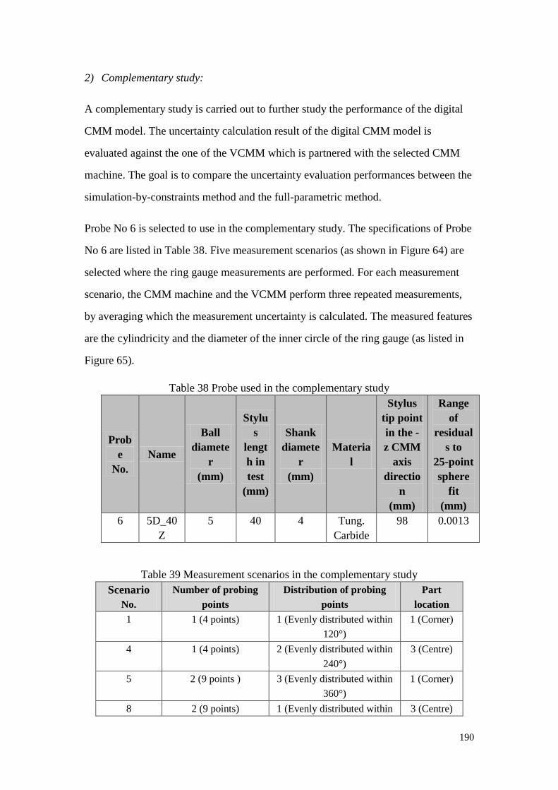
190

2) Complementary study:

A complementary study is carried out to further study the performance of the digital

CMM model. The uncertainty calculation result of the digital CMM model is

evaluated against the one of the VCMM which is partnered with the selected CMM

machine. The goal is to compare the uncertainty evaluation performances between the

simulation-by-constraints method and the full-parametric method.

Probe No 6 is selected to use in the complementary study. The specifications of Probe

No 6 are listed in Table 38. Five measurement scenarios (as shown in Figure 64) are

selected where the ring gauge measurements are performed. For each measurement

scenario, the CMM machine and the VCMM perform three repeated measurements,

by averaging which the measurement uncertainty is calculated. The measured features

are the cylindricity and the diameter of the inner circle of the ring gauge (as listed in

Figure 65).

Table 38 Probe used in the complementary study

Prob

e

No.

Name

Ball

diamete

r

(mm)

Stylu

s

lengt

h in

test

(mm)

Shank

diamete

r

(mm)

Materia

l

Stylus

tip point

in the -

z CMM

axis

directio

n

(mm)

Range

of

residual

s to

25-point

sphere

fit

(mm)

6 5D_40

Z

5 40 4 Tung.

Carbide

98 0.0013

Table 39 Measurement scenarios in the complementary study

Scenario

No.

Number of probing

points

Distribution of probing

points

Part

location

1 1 (4 points) 1 (Evenly distributed within

120°)

1 (Corner)

4 1 (4 points) 2 (Evenly distributed within

240°)

3 (Centre)

5 2 (9 points ) 3 (Evenly distributed within

360°)

1 (Corner)

8 2 (9 points) 1 (Evenly distributed within 3 (Centre)

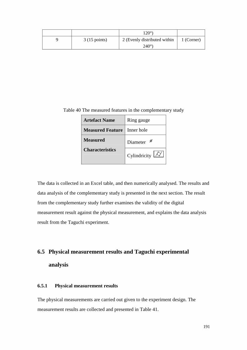
191

120°)

9 3 (15 points) 2 (Evenly distributed within

240°)

1 (Corner)

Table 40 The measured features in the complementary study

Artefact Name Ring gauge

Measured Feature Inner hole

Measured

Characteristics

Diameter

Cylindricity

The data is collected in an Excel table, and then numerically analysed. The results and

data analysis of the complementary study is presented in the next section. The result

from the complementary study further examines the validity of the digital

measurement result against the physical measurement, and explains the data analysis

result from the Taguchi experiment.

6.5 Physical measurement results and Taguchi experimental

analysis

6.5.1 Physical measurement results

The physical measurements are carried out given to the experiment design. The

measurement results are collected and presented in Table 41.

192

Table 41 Data collection for physical measurement results

Ru

n

No.

Measurement scenarios Diameter Cylindricity

Probe

specificati

on

Numb

er of

probi

ng

points

Distributi

on of

probing

points

Part

locati

on

Uncertai

nty

X_

val

ue

Y_

val

ue

Uncertai

nty

1 1pt3D_22

Z 4 120

Corne

r 0.8 0.1 0.9 0.906

2 1pt3D_22

Z 4 120

Corne

r 0.6 0.2 0.7 0.728

3 1pt3D_22

Z 4 120

Corne

r 1.1 0.5 0.9 1.030

4 1pt3D_22

Z 9 240

Middl

e 0.9 0.1 0.6 0.608

5 1pt3D_22

Z 9 240

Middl

e 0.4 0 0.4 0.400

6 1pt3D_22

Z 9 240

Middl

e 0.7 0.1 0.6 0.608

7 1pt3D_22

Z 15 360 Centre 0.1 0.1 0.1 0.141

8 1pt3D_22

Z 15 360 Centre 0 0 0 0.000

9 1pt3D_22

Z 15 360 Centre 0.1 0 0.1 0.100

10 3D_78Z 4 240 Centre 0.1 0.1 0.2 0.224

11 3D_78Z 4 240 Centre 0.1 0 0 0.000

12 3D_78Z 4 240 Centre 0.2 0 0.1 0.100

13 3D_78Z 9 360 Corne

r 0.2 0 0.1 0.100

14 3D_78Z 9 360 Corne

r 0.2 0 0 0.000

15 3D_78Z 9 360 Corne

r 0.1 0 0 0.000

16 3D_78Z 15 120 Middl

e 0.3 1 0 1.000

17 3D_78Z 15 120 Middl

e 0.3 0.1 0.1 0.141

18 3D_78Z 15 120 Middl

e 3 1 0 1.000

19 5D_40Z 4 360 Middl

e 0.3 0.1 0.1 0.141

193

20 5D_40Z 4 360 Middl

e 0.2 0.1 0.1 0.141

21 5D_40Z 4 360 Middl

e 0.4 0.2 0.1 0.224

22 5D_40Z 9 120 Centre 0.1 0.1 0.2 0.224

23 5D_40Z 9 120 Centre 0.1 0.1 0.2 0.224

24 5D_40Z 9 120 Centre 0 0.1 0.2 0.224

25 5D_40Z 15 240 Corne

r 0.1 0.1 0.1 0.141

26 5D_40Z 15 240 Corne

r 0.2 0.1 0.1 0.141

27 5D_40Z 15 240 Corne

r 0.1 0.1 0 0.100

6.5.2 Taguchi experimental analysis of physical measurement results

The main effects plots of the means and S/N ratios are generated versus the control

factors. The linear model results for S/N ratios and means are displayed with respects

to diameter measurements and cylindricity measurements in the physical

measurement environment.

1) Diameter analysis result

The Taguchi analysis results of diameter measurements in the physical measurement

environment are summarized in Table 42 and Table 44. Table 42 shows the response

table and main effects plot for the means, and Table 44 shows the response table and

main effects plot for the S/N ratios. The interpretations of Table 42 and Table 44 are

presented in the following paragraphs.

A. The effects of the control factors on the mean values

Table 42 reveals the effects of the selected control factors on the mean values of

measurement uncertainty by measuring the diameter of the ring gauge in the physical

measurement environment.

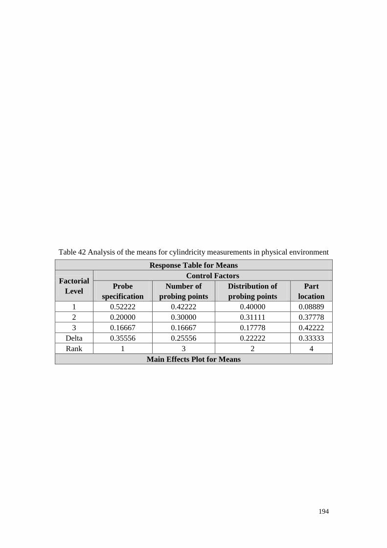
194

Table 42 Analysis of the means for cylindricity measurements in physical environment

Response Table for Means

Factorial

Level

Control Factors

Probe

specification

Number of

probing points

Distribution of

probing points

Part

location

1 0.52222 0.42222 0.40000 0.08889

2 0.20000 0.30000 0.31111 0.37778

3 0.16667 0.16667 0.17778 0.42222

Delta 0.35556 0.25556 0.22222 0.33333

Rank 1 3 2 4

Main Effects Plot for Means

195

5D_40Z3D_78Z1pt3D_22Z

0.5

0.4

0.3

0.2

0.1

1594

360240120

0.5

0.4

0.3

0.2

0.1

CornerMiddleCentre

Probe specification

Me

an

of

Me

an

s

Number of probing points

Distribution of probing points Part location

Main Effects Plot for MeansData Means

Key words: physical measurement, diameter, mean

From the ‘Main Effects Plot for Mean’ in Table 42, two tendencies are observed: a)

the diameter measurement is influenced by the selected measurement uncertainty

contributors; b) Different measurement uncertainty contributors have different effects

on the diameter measurement results. These two points are described and discussed

into more details in the following paragraphs.

a) The diameter measurement is influenced by the selected measurement uncertainty

contributors. The mean value of the diameter measurement uncertainties,

determined from the physical measurements, changes over the changes of ‘probe

specification’, ‘number of probing points’, ‘distribution of probing points’ and

‘part location’. Several points are made by examining the ‘Main Effects Plot for

Mean’ against the control factors:

Probe specification: The mean value of measurement uncertainty decreases

significantly when it is switched to better CMM probe. In particularly, the

measurement uncertainty reduces significantly between Probe 1pt3D_22Z and

3D_78Z. The Taguchi analysis result of the factor effect conforms to common

understandings on CMM measurement.

Number of probing points: The mean value of measurement uncertainty

196

decreases when the number of probing points increases. The measurement

results are improved by probing more points on the feature. The Taguchi

analysis result of the factor effect fairly conforms to common understandings

on CMM measurement. NPL suggests probing 7 points for circle measurement

[135], beyond which the number of probing points has less effects on

measurement result.

Distribution of probing points: The mean value of measurement uncertainty

decreases as the probing points are distributed more evenly around the circle.

The Taguchi analysis result of the factor effect conforms to common

understandings on CMM measurement.

Part location: The mean value of measurement uncertainty decreases, as the

part is moved toward to the centre of the CMM bed. The Taguchi analysis

result of the factor effect conforms to common understandings on CMM

measurement.

b) Different measurement uncertainty contributors have different effects on the

diameter measurement results. The range of the measurement uncertainty change

varies between the selected control factors. The ranks of the factor effects are

assigned based on Delta statistics calculation, and are presented in the ‘Response

Table for Means’ in Table 42.

From Table 42, it can be seen that ‘probe specification’ has the greatest effect on

the mean value of measurement uncertainty. ‘Distribution of probing points’ has

the second greatest effect, followed by ‘number of probing points’ and ‘part

location’. The rank is fairly consistent with the common understandings on CMM

measurement. The rank of the control factor effects is discussed in Table 43.

Table 43 Discussions of the control factor effects on diameter measurements in the

physical environment

Rank Factor Discussion

197

1 Probe specification Consistent with common understanding on CMM

measurement. The quality of measurement hardware

assets is primary to the measurement result

2 Distribution of

probing points

Consistent with common understanding on CMM

measurement. The even distribution of probing points

is essential for circle measurement, and the probing

points are impelled to be evenly distributed.

3 Number of probing

points

Raising concern. The ‘number of probing points’

should have less effect on measurement result in this

physical experiment.

4 Part location Raising concern because of the concern from ‘number

of probing points’ effect. The ranks of ‘part location’

and ‘number of probing points’ are not consistent with

common understandings on CMM measurement.

B. The effects of the control factors on the S/N ratios

Table 44 reveals the effects of the selected control factors on the S/N ratios of

measurement uncertainty by measuring the diameter of the ring gauge in the physical

measurement environment.

198

Table 44 Analysis of the S/N ratios for diameter measurements in physical

environment

Response Table for S/N Ratios

Factorial

Level

Control Factors

Probe

specification

Number of

probing points

Distribution of

probing points

Part

location

1 16.25 18.92 18.38 24.77

2 24.77 20.51 20.51 20.51

3 23.18 24.77 23.18 15.99

Delta 8.53 5.85 4.80 8.78

Rank 2 3 4 1

Main Effects Plot for S/N Ratios

5D_40Z3D_78Z1pt3D_22Z

25.0

22.5

20.0

17.5

15.0

1594

360240120

25.0

22.5

20.0

17.5

15.0

CornerMiddleCentre

Probe specification

Me

an

of

SN

ra

tio

s

Number of probing points

Distribution of probing points Part location

Main Effects Plot for SN ratiosData Means

Signal-to-noise: Nominal is best (-10*Log10(s**2))

Key words: physical measurement, diameter, S/N ratio

Table 44 shows fairly good S/N ratios for diameter measurement. It indicates that

the four control factors have significant impacts on the CMM measurement

uncertainty, and are fairly independent from other measurement uncertainty

contributors. Noticeably, the S/N ratio in physical measurements varies greatly

against the factorial level changes. It indicates that the physical measurement

environment is influenced by more measurement uncertainty contributors. Similar

to the digital measurement environment, the ‘probe specification’ has greater

impact on the S/N ratio, because the ‘probe specification’ is composed by three

components, ‘stylus length in test’, ‘stylus tip point in the - z CMM axis direction’

199

and ‘range of residuals to 25-point sphere fit’, which possibly contribute more

noises over the measurement process.

To conclude, the above Taguchi analysis have produced fairly reasonable results in

predicting the effects of the control factors on measurement uncertainty of the

diameter measurements in physical environment. But the effect of ‘number of probing

points’ does not approve the NPL experimental result [135], and the disapproval can

not be explained.

2) Cylindricity analysis result

The Taguchi analysis results of cylindricity measurements in physical measurement

environment are summarized in Table 45 and Table 46. Table 45 shows the response

table and main effects plot for the means, and Table 46 shows the response table and

main effects plot for the S/N ratios. The interpretations of Table 45 and Table 46 are

presented in the following paragraphs.

A. The effects of the control factors on the mean values

Table 45 reveals the effects of the selected control factors on the mean values of

measurement uncertainty by measuring the cylindricity of the ring gauge in the

physical measurement environment.

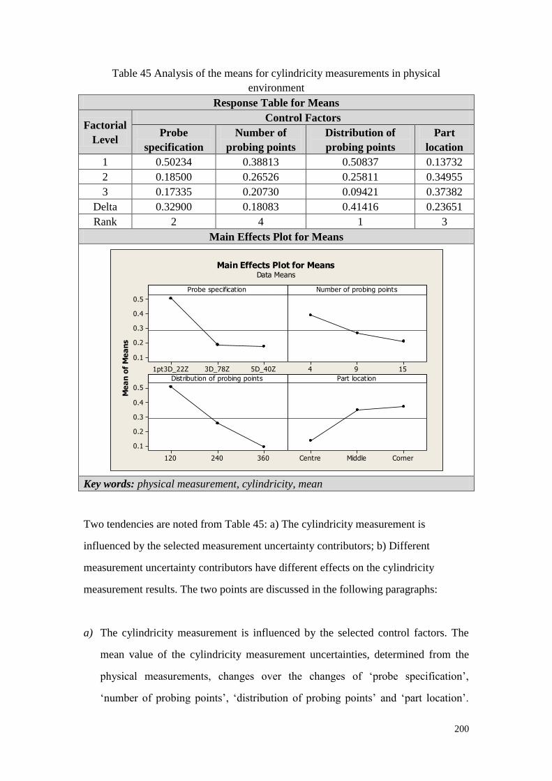
200

Table 45 Analysis of the means for cylindricity measurements in physical

environment

Response Table for Means

Factorial

Level

Control Factors

Probe

specification

Number of

probing points

Distribution of

probing points

Part

location

1 0.50234 0.38813 0.50837 0.13732

2 0.18500 0.26526 0.25811 0.34955

3 0.17335 0.20730 0.09421 0.37382

Delta 0.32900 0.18083 0.41416 0.23651

Rank 2 4 1 3

Main Effects Plot for Means

5D_40Z3D_78Z1pt3D_22Z

0.5

0.4

0.3

0.2

0.1

1594

360240120

0.5

0.4

0.3

0.2

0.1

CornerMiddleCentre

Probe specification

Me

an

of

Me

an

s

Number of probing points

Distribution of probing points Part location

Main Effects Plot for MeansData Means

Key words: physical measurement, cylindricity, mean

Two tendencies are noted from Table 45: a) The cylindricity measurement is

influenced by the selected measurement uncertainty contributors; b) Different

measurement uncertainty contributors have different effects on the cylindricity

measurement results. The two points are discussed in the following paragraphs:

a) The cylindricity measurement is influenced by the selected control factors. The

mean value of the cylindricity measurement uncertainties, determined from the

physical measurements, changes over the changes of ‘probe specification’,

‘number of probing points’, ‘distribution of probing points’ and ‘part location’.

201

Several points are made by examining the ‘Main Effects Plot for Mean’ against

the control factors:

Probe specification: The mean value of measurement uncertainty decreases

significantly when it is switched to better CMM probe. In particularly, the

measurement uncertainty reduces significantly between Probe 1pt3D_22Z and

3D_78Z. The Taguchi analysis result of the factor effect conforms to common

understandings on CMM measurement.

Number of probing points: The mean value of measurement uncertainty

decreases when the number of probing points increases. The measurement

results are improved by probing more points on the feature. The Taguchi

analysis result of the factor effect conforms to common understandings on

CMM measurement.

Distribution of probing points: The mean value of measurement uncertainty

decreases fairly significantly, when the probing points are distributed more

evenly around the circle. The Taguchi analysis result of the factor effect

conforms to common understandings on CMM measurement.

Part location: The mean value of measurement uncertainty decreases, as the

part is moved toward to the centre of the CMM bed. In particularly, the

measurement uncertainty reduces more significantly when the part is moved

from the ‘middle’ point to the centre of the CMM bed. The Taguchi analysis

result of the factor effect conforms to common understandings on CMM

measurement.

b) Different measurement uncertainty contributors have different effects on the

cylindricity measurement results. The range of the measurement uncertainty

change varies between the selected control factors.

From Table 45, it can be seen that ‘Distribution of probing points’ has the greatest

effect on the mean value of measurement uncertainty. ‘Probe specification’ has

the second greatest effect, followed by ‘number of probing points’ and ‘part

202

location’. This Taguchi analysis result suggests that, the most effective way to

minimize the measurement uncertainty is to encourage an even distribution of

probing points, and the second effective way is to switch to a better CMM probe.

Increasing the density of probing points is also effective, but not as effective as

the former two options. Positioning the part in the centre of CMM bed has least

effective impact.

B. The effects of the control factors on the S/N ratios

Table 46 reveals the effects of the selected control factors on the S/N ratios of

measurement uncertainty of cylindricity measurements in the physical environment.

203

Table 46 Analysis of the S/N ratios for cylindricity measurements in physical

environment

Response Table for S/N Ratios

Factorial

Level

Control Factors

Probe

specification

Number of

probing points

Distribution of

probing points

Part

location

1 9.754 8.683 109.977 105.639

2 -2.294 108.206 9.082 8.376

3 113.977 4.548 2.378 7.423

Delta 116.270 103.658 107.599 98.216

Rank 1 3 2 4

Main Effects Plot for S/N Ratios

5D_40Z3D_78Z1pt3D_22Z

100

75

50

25

0

1594

360240120

100

75

50

25

0

CornerMiddleCentre

Probe specification

Me

an

of

SN

ra

tio

s

Number of probing points

Distribution of probing points Part location

Main Effects Plot for SN ratiosData Means

Signal-to-noise: Nominal is best (10*Log10(Ybar**2/s**2))

Key words: physical measurement, cylindricity, S/N ratio

Table 46 shows fairly good S/N ratios for cylindricity measurement. The four control

factors have significant impacts on the CMM measurement uncertainty, and they are

fairly independent. The variance of S/N ratios in the physical measurements is

generally higher than in the digital measurements.

The above Taguchi analysis has produced reasonable results in predicting the effects of

the control factors on measurement uncertainty for the cylindricity measurements in the

physical environment.

204

6.5.3 Conclusion of Taguchi experiment method in physical environment

The physical measurement results are collected and analysed using Taguchi data

analysis method. The control factor effects on the mean values and S/N ratios are

deliberately examined. The Taguchi analysis results have produced reasonable results

in predicting the effects of the control factors on measurement uncertainty for both of

diameter and cylindricity measurements in physical environment.

There are defects in the Taguchi analysis results. These defects build on the high

complexity of CMM measurement tasks. The complete traceability of uncertainty

chain is virtually impossible to model and manage. Despite the defects, the physical

measurement results are still of very high quality. The Taguchi analysis results from

the physical measurements are used to benchmark that from the digital measurements,

and therefore to verify the digital CMM measurement model.

The comparisons between digital and physical measurements are provided in the next

section.

6.6 Comparison between physical measurement results and digital

measurement results

The digital measurement results and the physical measurement results are compared

in this section in order to assess the validity of the Measurement Planning and

Implementation Framework. Firstly, the two sets of measurement results are

compared directly under each measurement scenario. The direct comparison concerns

the verification of the digital CMM model. Secondly, the two sets of Taguchi analysis

results are compared. This comparison assesses the validity of the Taguchi analysis

method proposed in the Framework.

6.6.1 Direct comparison

205

In this section, the digital measurement results and physical measurement results are

compared for the two feature measurements, diameter and cylindricity.

1) Diameter measurements

Table 47 ties the digital measurement results and the physical measurement results.

The measurement results in Table 47 are the average value of the three measurement

runs for each measurement scenario. The ratios the digital measurement results and

the physical measurement results are calculated and listed in the last row of Table 47.

Figure 80 is constructed based on Table 47.

206

Table 47 Data collection for comparing diameter measurement results

Measurement

Scenario No.

Measurement Uncertainty Contributors Diameter

Probe

specification

Number of

probing points

Distribution of

probing points

Part

location

Average of digital

measurement results

Average of physical

measurement results Ratio

1 1pt3D_22Z 4 120 Corner 21.171 0.833 25.405

2 1pt3D_22Z 9 240 Middle 15.850 0.667 23.775

3 1pt3D_22Z 15 360 Centre 13.734 0.067 206.010

4 3D_78Z 4 240 Centre 7.450 0.133 55.878

5 3D_78Z 9 360 Corner 8.245 0.167 49.468

6 3D_78Z 15 120 Middle 10.173 0.300 33.910

7 5D_40Z 4 360 Middle 6.827 0.300 22.756

8 5D_40Z 9 120 Centre 8.781 0.067 131.720

9 5D_40Z 15 240 Corner 6.780 0.133 50.850

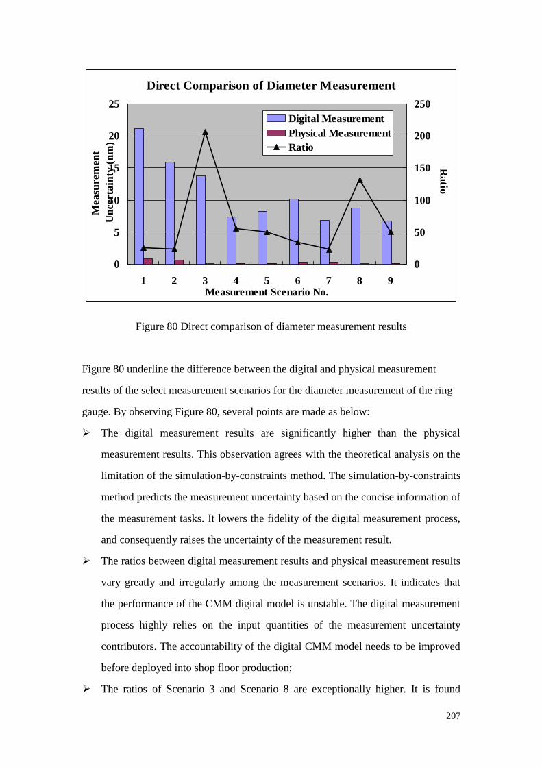
207

Direct Comparison of Diameter Measurement

0

5

10

15

20

25

1 2 3 4 5 6 7 8 9Measurement Scenario No.

Mea

surem

en

t

Un

certa

inty

(n

m)

0

50

100

150

200

250R

atio

Digital Measurement

Physical Measurement

Ratio

Figure 80 Direct comparison of diameter measurement results

Figure 80 underline the difference between the digital and physical measurement

results of the select measurement scenarios for the diameter measurement of the ring

gauge. By observing Figure 80, several points are made as below:

The digital measurement results are significantly higher than the physical

measurement results. This observation agrees with the theoretical analysis on the

limitation of the simulation-by-constraints method. The simulation-by-constraints

method predicts the measurement uncertainty based on the concise information of

the measurement tasks. It lowers the fidelity of the digital measurement process,

and consequently raises the uncertainty of the measurement result.

The ratios between digital measurement results and physical measurement results

vary greatly and irregularly among the measurement scenarios. It indicates that

the performance of the CMM digital model is unstable. The digital measurement

process highly relies on the input quantities of the measurement uncertainty

contributors. The accountability of the digital CMM model needs to be improved

before deployed into shop floor production;

The ratios of Scenario 3 and Scenario 8 are exceptionally higher. It is found

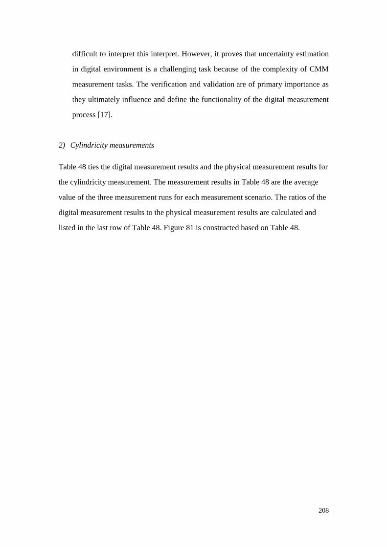
208

difficult to interpret this interpret. However, it proves that uncertainty estimation

in digital environment is a challenging task because of the complexity of CMM

measurement tasks. The verification and validation are of primary importance as

they ultimately influence and define the functionality of the digital measurement

process [17].

2) Cylindricity measurements

Table 48 ties the digital measurement results and the physical measurement results for

the cylindricity measurement. The measurement results in Table 48 are the average

value of the three measurement runs for each measurement scenario. The ratios of the

digital measurement results to the physical measurement results are calculated and

listed in the last row of Table 48. Figure 81 is constructed based on Table 48.

209

Table 48 Data collection for comparing cylindricity measurement results

Measurement

Scenario No.

Measurement Uncertainty Contributors Diameter

Probe

specification

Number of

probing

points

Distribution of

probing points

Part

location

Average of digital

measurement results

Average of physical

measurement results Ratio

1 1pt3D_22Z 4 120 Corner 13.847 0.888 15.599

2 1pt3D_22Z 9 240 Middle 8.489 0.539 15.753

3 1pt3D_22Z 15 360 Centre 3.235 0.080 40.199

4 3D_78Z 4 240 Centre 3.700 0.108 34.300

5 3D_78Z 9 360 Corner 3.666 0.033 109.980

6 3D_78Z 15 120 Middle 5.380 0.414 13.002

7 5D_40Z 4 360 Middle 2.685 0.169 15.905

8 5D_40Z 9 120 Centre 5.317 0.224 23.777

9 5D_40Z 15 240 Corner 4.176 0.128 32.724

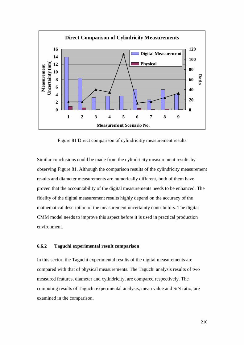
210

Direct Comparison of Cylindricity Measurements

0

2

4

6

8

10

12

14

16

1 2 3 4 5 6 7 8 9

Measurement Scenario No.

Mea

surem

en

t

Un

certa

inty

(n

m)

0

20

40

60

80

100

120

Ra

tio

Digital Measurement

Physical

MeasurementRatio

Figure 81 Direct comparison of cylindricitiy measurement results

Similar conclusions could be made from the cylindricity measurement results by

observing Figure 81. Although the comparison results of the cylindricity measurement

results and diameter measurements are numerically different, both of them have

proven that the accountability of the digital measurements needs to be enhanced. The

fidelity of the digital measurement results highly depend on the accuracy of the

mathematical description of the measurement uncertainty contributors. The digital

CMM model needs to improve this aspect before it is used in practical production

environment.

6.6.2 Taguchi experimental result comparison

In this sector, the Taguchi experimental results of the digital measurements are

compared with that of physical measurements. The Taguchi analysis results of two

measured features, diameter and cylindricity, are compared respectively. The

computing results of Taguchi experimental analysis, mean value and S/N ratio, are

examined in the comparison.

211

1) Diameter measurement

Table 49 ties the Taguchi analysis results of the diameter measurements in the digital

environment and the physical environment. The rows of ‘Mean’ and ‘S/N Ratio’

respectively contain the Taguchi analysis results of the mean values and of the S/N

ratios from the two measurement environments.

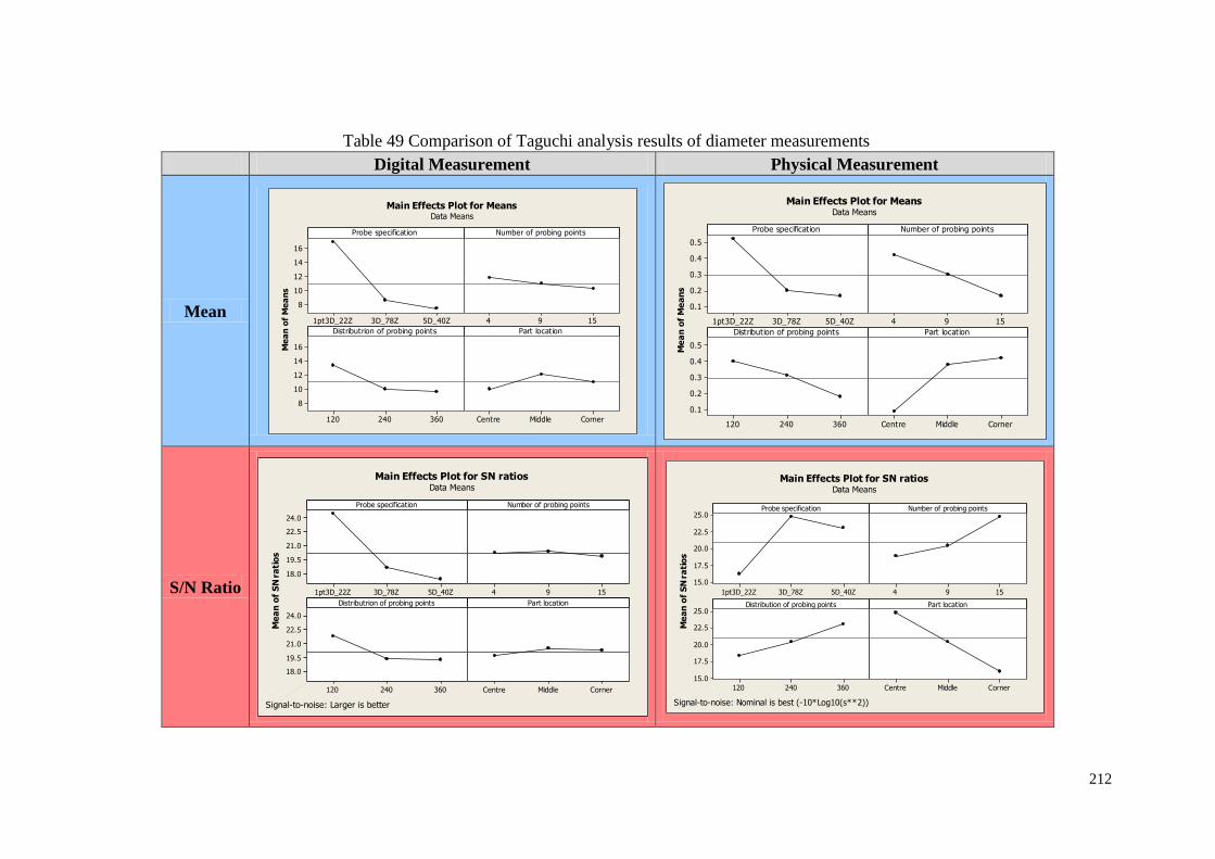
212

Table 49 Comparison of Taguchi analysis results of diameter measurements

Digital Measurement Physical Measurement

Mean 5D_40Z3D_78Z1pt3D_22Z

16

14

12

10

8

1594

360240120

16

14

12

10

8

CornerMiddleCentre

Probe specification

Me

an

of

Me

an

s

Number of probing points

Distributrion of probing points Part location

Main Effects Plot for MeansData Means

5D_40Z3D_78Z1pt3D_22Z

0.5

0.4

0.3

0.2

0.1

1594

360240120

0.5

0.4

0.3

0.2

0.1

CornerMiddleCentre

Probe specification

Me

an

of

Me

an

s

Number of probing points

Distribution of probing points Part location

Main Effects Plot for MeansData Means

S/N Ratio 5D_40Z3D_78Z1pt3D_22Z

24.0

22.5

21.0

19.5

18.0

1594

360240120

24.0

22.5

21.0

19.5

18.0

CornerMiddleCentre

Probe specification

Me

an

of

SN

ra

tio

s

Number of probing points

Distributrion of probing points Part location

Main Effects Plot for SN ratiosData Means

Signal-to-noise: Larger is better

5D_40Z3D_78Z1pt3D_22Z

25.0

22.5

20.0

17.5

15.0

1594

360240120

25.0

22.5

20.0

17.5

15.0

CornerMiddleCentre

Probe specification

Me

an

of

SN

ra

tio

s

Number of probing points

Distribution of probing points Part location

Main Effects Plot for SN ratiosData Means

Signal-to-noise: Nominal is best (-10*Log10(s**2))

213

Comparison of mean values

As shown in Table 49, the mean values from the digital measurements are

generally higher than that from the physical measurements. It indicates that the

simulation-by-constraints method tends to overstate the measurement uncertainty.

This problem is caused by the nature of the simulation-by-constraints method,

which requires the partial information feed of the measurement task. It suggests

the end-users to provide as fully complete description of CMM measurement

scenarios as possible to the digital CMM model. On the other hand, it implicates

that the simulation-by-constraints method is possibly more appropriate for

instructing CMM measurement process than merely evaluating the measurement

uncertainty of specific CMM measurement task.

For the diameter measurements, the trends of the mean value changing against the

control factors show noticeable consistency between the digital measurement

results and the physical measurement results. Several points are made by

comparing the mean value trends against the selected control factors:

Probe Specification: The mean values of measurement uncertainty decrease

as switching to better probe. The measurement uncertainty decreases more

significantly between Probe 1pt3D_22Z and Probe 3D_78Z. The trend in

digital measurements is consistent with that in physical measurements.

Number of probing points: The mean values of measurement uncertainty

decrease as the number of probing points increase. The mean value of

measurement uncertainty in physical environment has bigger variation against

the factorial level changes than that in digital environment. The trend in digital

measurements is generally consistent with that in physical measurement. But

intensifying the probing points is more effective in the physical measurement

environment than in the digital measurement environment. It implicates that

the simulation-by-constraints method is less sensitive on individual

uncertainty contributors because of its nature.

Distribution of probing points: The mean value of measurement uncertainty

214

decreases as the probing points is distributed more evenly along the circle. The

trend in digital measurements is fairly consistent with that in physical

measurements.

Part location: In the digital measurement environment, the measurement

uncertainty is at the peak when the part is located at the quarter of the diagonal

line of the CMM bed. However, in the physical measurement results, the

measurement uncertainty increases greatly as the part moves from the centre

to the corner of the CMM bed. The trend in digital measurements is

inconsistent with that in physical measurement. The digital measurement

results deviate from common understanding of CMM measurement process,

and therefore are identified as bad data. The trend comparison of ‘part

location’ indicates the limited nature of the simulation-by-constraints method,

but does not refute the feasibility of Taguchi analysis approach proposed in

this research.

From the Taguchi analysis on the physical measurement results, it could be seen

that the ‘probe specification’ factor has the biggest impact on the measurement

result. The ‘part location’ factor has second biggest impact. The rest of the two

factors have similar impact, while the ‘number of probing points’ has slightly

bigger impact than ‘distribution of probing points’. The Taguchi analysis on the

digital measurement results shows fairly logical coherence with the physical ones,

but also shows certain degree of misalignment. The ‘probe specification’ has the

biggest impact, which is the same with the analysis on the physical measurements.

Although the analysis on digital measurements shows that the ‘distribution of

probing points’ has the second biggest impact on measurement uncertainty, the

impacts of ‘number of probing points’ is not significantly lower than that of

‘distribution of probing points’. This is similar to the analysis on the digital

measurements. The digital analysis result of ‘part location’ is inconsistent with

common sense of CMM measurement, and consequently it is not proper to refer

the ‘part location’ analysis result for the comparison. However, it suggests that

215

the digital CMM model needs to improve its sensibility on the part location

change.

Comparison of S/N ratios

In general Taguchi experimental design, S/N ratio reflects the robustness of the

experiment process and analysis result. In this Taguchi experimental design, S/N

ratio is neither the key index for assessing the capability of the digital CMM

model and nor for validating the Measurement Planning and Implementation

Framework. Given the aims and objectives of this experimental research, it is not

necessary to compare the S/N ratio values between the digital measurement

environment and the physical measurement environment.

The S/N ratios are discussed here in order to examine the robustness of the

Taguchi experimental approach proposed in this research, in particular, to

indentify the effects of the selected control factors on the measurement

uncertainty against the un-selected control factors (other measurement uncertainty

contributors).

As shown in Table 49, the S/N ratios in both of digital and physical environments

show good values, varying between 15 to 25. It confirms the robustness of the

Taguchi experimental design in both of the digital measurement environment and

the physical environment. Moreover, it indicates the prospect of incorporating the

design of experiments (DOE) methods into the measurement uncertainty analysis

to enable the knowledge management in task-specific measurements and to create

the adoption of measurement experiences to the overall manufacturing process

control.

2) Cylindricity measurement

216

Table 50 ties the Taguchi analysis results of the cylindricity measurements in the

digital environment and the physical environment.

217

Table 50 Comparison of Taguchi analysis results of cylindricity measurements

Digital Measurement Physical Measurement

Mean 5D_40Z3D_78Z1pt3D_22Z

9.0

7.5

6.0

4.5

3.0

1594

360240120

9.0

7.5

6.0

4.5

3.0

CornerMiddleCentre

Probe specification

Me

an

of

Me

an

s

Number of probing points

Distributrion of probing points Part location

Main Effects Plot for MeansData Means

5D_40Z3D_78Z1pt3D_22Z

0.5

0.4

0.3

0.2

0.1

1594

360240120

0.5

0.4

0.3

0.2

0.1

CornerMiddleCentre

Probe specification

Me

an

of

Me

an

s

Number of probing points

Distribution of probing points Part location

Main Effects Plot for MeansData Means

S/N Ratio 5D_40Z3D_78Z1pt3D_22Z

18

16

14

12

10

1594

360240120

18

16

14

12

10

CornerMiddleCentre

Probe specification

Me

an

of

SN

ra

tio

s

Number of probing points

Distributrion of probing points Part location

Main Effects Plot for SN ratiosData Means

Signal-to-noise: Larger is better

5D_40Z3D_78Z1pt3D_22Z

100

75

50

25

0

1594

360240120

100

75

50

25

0

CornerMiddleCentre

Probe specification

Me

an

of

SN

ra

tio

s

Number of probing points

Distribution of probing points Part location

Main Effects Plot for SN ratiosData Means

Signal-to-noise: Nominal is best (10*Log10(Ybar**2/s**2))

218

Comparison of mean values

Table 50 shows that the mean values of the cylindricity measurements in the

digital environment are generally higher than that in the physical environment.

This is similar to the diameter measurements, and once again indicates that the

simulation-by-constraints method tends to overstate the measurement uncertainty.

For the cylindricity measurements, the trends of the mean value changing against

the control factors also show good consistency between the digital measurement

results and the physical measurement results. Several points are made by

comparing the mean value trends against the selected control factors:

Probe Specification: The mean values of measurement uncertainty decrease

as switching to better probe. The measurement uncertainty decreases more

significantly between Probe 1pt3D_22Z and Probe 3D_78Z. The trend in

digital measurements is consistent with that in physical measurements.

Number of probing points: The mean values of measurement uncertainty

decrease as the number of probing points increase. The trend in digital

measurements is consistent with that in physical measurements.

Distribution of probing points: The mean value of measurement uncertainty

decreases as the probing points is distributed more evenly along the circle. The

trend in digital measurements is consistent with that in physical

measurements.

Part location: In the digital measurement environment, the measurement

uncertainty is at the peak when the part is located at the quarter of the diagonal

line of the CMM bed. However, in the physical measurement results, the

measurement uncertainty increases greatly as the part moves from the centre

to the corner of the CMM bed. The trend in digital measurements is

inconsistent with that in physical measurement. The digital measurement

results deviate from common understanding of CMM measurement process,

and therefore are identified as bad data. The trend comparison of ‘part

location’ indicates the limited nature of the simulation-by-constraints method,

219

but does not refute the feasibility of Taguchi analysis approach proposed in

this research.

Similar comparison results are observed from the cylindricity measurements as

from the diameter measurements. In the physical measurement environment, the

‘distribution of probing points’ factor has the biggest impact on the measurement

result for cylindricity measurement. The ‘probe specification’ factor has second

biggest impact, followed by ‘part location’ and ‘number of probing points’. The

Taguchi analysis on the digital measurement results shows logical coherence with

the physical ones, although has slight misalignment on the ‘part location’ factor.

The analysis results from the digital measurements have the same patterns with

the ones from physical measurements in terms of ‘probe specification’,

‘distribution of probing points’ and ‘number of probing points’. In the digital

analysis results, the ‘distribution of probing points’ factor has the biggest impact

on the measurement uncertainty, followed by ‘probe specification’ and ‘number

of probing points’. The digital measurement results of ‘part location’ are

inconsistent with common sense of CMM measurement, and consequently it is

not proper to refer the ‘part location’ analysis result for the comparison.

Therefore, generally speaking, the control factor rank obtained from the digital

measurements is aligned with that from the physical measurements. The approach

proposed in the Measurement Planning and Implementation Framework has been

validated and verified in the physical environment by measuring the cylindricity

of the ring gauge using the procedures in this experiment design. To a certain

degree, it is proved that the Framework, which statistically analyses the

task-specific measurement uncertainty calculated by the digital CMM model, is

capable to provide closer integration between digital and physical measurement

environments.

220

In addition, the Framework strengthens the ability of the digital CMM model in

measuring form tolerances. Although the digital measurement result and the

physical measurement result are significantly different for the cylindricity

measurements in this research, the Taguchi analysis results on both of the digital

measurements and the physical measurements reveal similar patterns indicating

the impact levels of the control factors.

Comparison of S/N ratios

As claimed in the previous paragraph, S/N ratio is not the key index for validating

the Measurement Planning and Implementation Framework in this Taguchi

experimental design. It is not necessary to compare the S/N ratio values between

the digital measurement environment and the physical measurement environment.

The S/N ratios are discussed here in order to examine the robustness of the

Taguchi experimental approach proposed in this research, in particular, for the

cylindricity measurements.

As shown in Table 50, the S/N ratios in both the digital and physical

environments reasonably high values. It confirms the robustness of the Taguchi

experimental design in both of the digital measurement environment and the

physical environment. Moreover, it indicates the prospect of incorporating the

design of experiments (DOE) methods into the measurement uncertainty analysis

to enable the knowledge management in task-specific measurement and to create

the adoption of measurement experiences to the overall manufacturing process

control.

6.6.3 Conclusion

In this section, the Taguchi analysis results from the digital and physical

measurements have been compared in terms of the diameter and cylindricity

measurements. The comparison shows generally positive results, proving promising

221

prospects of the Measurement Planning and Implementation Framework for

integrating digital and physical measurement results.

The comparison results indicate the interesting points regarding the digital

measurements and verification. The accountability of the digital CMM model needs to

improve, especially in the regard of sensing the part location change on the CMM bed.

Although the direct comparison shows that the digital CMM model is not capable of

predicting form measurement results, the Taguchi analysis results on both of the

digital measurements and the physical measurements reveal similar patterns

indicating the impact levels of the control factors. The Framework strengthens the

ability of the digital CMM model in measuring form tolerances.

The relatively high S/N ratios from the Taguchi experiment design prove the

robustness of the Framework. It indicates the prospect of incorporating the design of

experiments (DOE) methods into the measurement uncertainty analysis, which will

enable the knowledge management in task-specific measurements and to create the

adoption of measurement experiences to the overall manufacturing process control.

6.7 Chapter Summary

In this Chapter, the experimental works to validate the Measurement Planning and

Implementation Framework have been carried out. The experimental plan has been

carefully designed, including selecting proper measured artifact, assessing available

measurement resources and defining the measurement uncertainty contributors.

Following the procedures in the experimental design, the digital measurements and

the physical measurements are carried out respectively. The results from the digital

measurements and the physical measurements have been collected and analyzed using

the approach proposed in the Framework. Finally, the measurement results and the

analyzed results have been compared respectively. The direct comparisons between

the digital and physical measurement results have shown that the digital measurement

222

generally produces higher measurement uncertainty than the physical measurement.

On the other hand, the Taguchi analyzing comparisons have shown good consistency

between the digital and physical measured results.

The Framework indicates a promising prospect of deploying the digital CMM model

in a shopfloor environment to direct measurement resource allocation. In this

environment, the measurement uncertainty contributors could be established on more

significant levels (e.g. temperature control and CMM machine). By analysing the

digital measurement results using the method in the Framework, the measurement

manager could estimate the significance levels of the measurement uncertainty

contributors, and decide the capital investments on the measurement capability

improvement and the production control.

Additionally, the scientific validation of the Framework shows an encouraging future

in the introduction of statistical methods to post-measurement data processing,

especially for digital measurement result analysis. By deploying proper statistical

methods, the digital measurement results could be used to direct the physical

measurement environment in a robust manner. It extends the application fields of the

digital CMM model. Moreover, it promotes the knowledge management in

task-specific measurements and creates the adoption of measurement experiences to

the overall manufacturing process control.

223

Chapter 7 Conclusions and Further Work

7.1 Conclusions

The developed Measurement Planning and Implementation Framework and the

stand-alone Quality Information Framework for CMM measurement processes are

considered to have met the research objectives given in Section 3.2. The primary aim

of developing a metrology-based process modelling framework for integrating digital

and physical measurement environments has been achieved. The workflow and the

general structure of the Framework have been given in Chapter 5. The four major

modules that form the Measurement Planning and Implementation Framework,

namely Measurement Scenario Streamliner Module, Measurement Uncertainty

Simulation Module, Physical Verification Process and Post-Measurement Data

Analysing Module, have been designed and implemented. A case study shown in

Chapter 6 has proved that the representation model of metrology-based process

modelling framework works correctly. Through the case study, the results form the

digital measurements and the physical measurements have been analyzed and

compared using the approach proposed in the Measurement Planning and

Implementation Framework. The comparisons have shown good consisteny between

the digital and physical measure results. It indicates the promising prospect of

introducing the statistical analysis approach into post-measurement uncertainty

processing, which will promote the knowledge management in task-specific

measurements and create the adoption of measurement experiences to the overall

manufacturing process control.

7.2 Contribution to knowledge

Evaluating measurement uncertainty in digital environments has been an established

topic in the metrology community. As shown in the literature review in Chapter 2,

224

many systems have been developed for measurement process modelling, and various

uncertainty estimation techniques have been deployed to calculate measurement

uncertainty in digital environments [4,12,13,14]. However, the integration between

digital and physical measurement environments is not fully verified, primarily

because of the large diversity and complexity of measurement tasks. It is virtually

impossible to develop an algorithm which considers all of the problems in the

measurement process. On the other hand, it tends to be impossible to verify the

performance of digital measurement models under all of the measurement scenarios.

From the literature review, these functions are not complete in the current research:

(1) Verification of digital measurement model performances in physical measurement

environments;

(2) Integration between digital and physical measurement environments in realistic

measurement scenarios;

(3) Robust framework which standardizes measurement process, and therefore, leads

measurement into manufacturing system integration.

Given the above points, the following contributions are considered to have been

made.

(1) The performance of a digital CMM model has been verified under meaningful

complexity measurement scenarios.

The physical measurements have been planned and carried out on a realistic

part in a shop floor environment;

The physical measurements have been simulated in the digital CMM model,

and generated simulation results;

The physical and digital measurement results have been compared directly;

225

The performance of the digital CMM model has been assessed, and the

limitations of the digital CMM model have been realized.

(2) A metrology-based process modeling framework for digital and physical

measurement environments integration has been developed.

The limitations of task-specific uncertainty simulation model have been

analyzed on technical level;

A Measurement Planning and Implementation Framework has been proposed.

The Framework analyzes measurement uncertainty to integrate digital and

physical measurement environments. And the statistical analyzing methods

and sophisticated algorithm models have been deployed in the Framework;

The experimental works to validate the Measurement Planning and

Implementation Framework have been carried out. Supplementary

capabilities of the digital CMM model have been discovered by the

experimental works. More importantly, the validation works have shown

good consistence between the digital and physical measure results by

deploying the Framework;

The validation work has indicated the promising prospect of introducing the

statistical analysis approach into post-measurement uncertainty processing,

which will extends the application fields of the measurement uncertainty

simulation model. Moreover, it promotes the knowledge management in

task-specific measurements and creates the adoption of measurement

experiences to the overall manufacturing process control.

226

7.3 Future work

The laboratory verification works have proved the validity of the proposed framework,

but future work is still required to increase the Framework capabilities as well as to

enhance the standardization and integration of measurement process modelling. The

recommendations for future work are included.

(1) Extension of the verification work to complex features

Limited by the availability of the physical measurement resources, the developed

Framework was verified by measuring a simple part. It is recommended to

expand the physical verification work to complex feature measurements, which

are highly demanded in high-value manufacturing.

(2) Extension of the verification work in shop floor environment

The scientific correctness of the proposed Framework has been verified in the

finely-controlled laboratory environment by delicate experiment design and

highly skilled metrology scientists. To enrich the industrial applicability of the

Framework, it is necessary to perform the physical measurements in the shop

floor environment to prove its validity in real production environment.

(3) Improvement of statistic methods for uncertainty analysis

The successful validation of the Framework has indicated the importance of

deploying statistic methods for post-measurement uncertainty analysis. Proper

deployment of statistics can release the practicality of measurement uncertainty in

real production environment, and improve the integration of measurement process

with overall product lifecycle. Future efforts should be paid to improve the

statistical methods for uncertainty analysis.

227

(4) Establishment of the relationship between the CMM measurement planning and

modelling to the Quality Information Framework (QIF)

The Quality Information Framework (QIF) is a robust conceptual framework

aiming to provide seamless data transition between the key stages of quality

measurement systems. [136].The QIF is expected to be the next generation

platform for integrating manufacturing quality systems based on the metrology

concepts

Relating the CMM measurement process planning with the QIF is vital for the

measurement process standardization, and the quality system integration. The

CMM measurement will get closer integration with the entire quality systems.

The CMM measurement modelling proposed in this research needs to be related

with the QIF module. And the validation of the QIF-derived CMM measurement

process modelling is needed to prove its functionality.

228

Appendix A. Data collection of the simulation results

Standard

Order

Run

Order

CMM

Specification Environment

Probing

Strategy

Diameter

(μm)

Position

(μm)

80 1 LA Shop Floor NPL 3.21 6.08

20 2 LA Enclosure NPL 1.35 4.32

5 3 HA CMM Room NPL 1.22 2.14

78 4 LA CMM Room 3*NPL 1.32 4.04

2 5 HA Enclosure NPL 0.665 1.48

37 6 MA Enclosure Minimum 1.01 2.52

28 7 HA Enclosure Minimum 0.753 1.56

57 8 HA Enclosure 3*NPL 0.604 1.39

41 9 MA CMM Room NPL 1.3 2.71

11 10 MA Enclosure NPL 0.816 2.27

24 11 LA CMM Room 3*NPL 1.38 4.18

72 12 MA Shop Floor 3*NPL 3.02 5.06

64 13 MA Enclosure Minimum 1.02 2.47

74 14 LA Enclosure NPL 1.41 4.16

56 15 HA Enclosure NPL 0.665 1.44

33 16 HA CMM Room 3*NPL 1.18 2.11

53 17 LA Shop Floor NPL 3.12 6.01

66 18 MA Enclosure 3*NPL 0.697 2.17

71 19 MA Shop Floor NPL 2.99 5.03

81 20 LA Shop Floor 3*NPL 3.12 5.8

21 21 LA Enclosure 3*NPL 0.98 4

1 22 HA Enclosure Minimum 0.748 1.54

54 23 LA Shop Floor 3*NPL 3.04 5.78

22 24 LA CMM Room Minimum 2.23 5.08

65 25 MA Enclosure NPL 0.831 2.29

75 26 LA Enclosure 3*NPL 0.988 3.52

59 27 HA CMM Room NPL 1.18 2.09

77 28 LA CMM Room NPL 1.69 4.36

23 29 LA CMM Room NPL 1.7 4.36

15 30 MA CMM Room 3*NPL 1.22 2.61

63 31 HA Shop Floor 3*NPL 2.89 4.66

17 32 MA Shop Floor NPL 3.07 5.04

67 33 MA CMM Room Minimum 1.44 2.93

35 34 HA Shop Floor NPL 2.97 4.8

70 35 MA Shop Floor Minimum 3.05 5.02

49 36 LA CMM Room Minimum 2.36 4.92

68 37 MA CMM Room NPL 1.26 2.71

19 38 LA Enclosure Minimum 1.97 4.82

45 39 MA Shop Floor 3*NPL 2.98 4.92

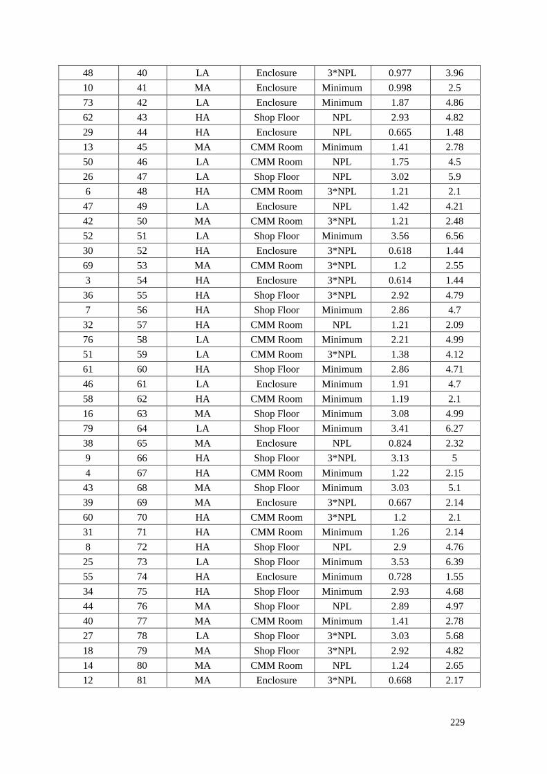
229

48 40 LA Enclosure 3*NPL 0.977 3.96

10 41 MA Enclosure Minimum 0.998 2.5

73 42 LA Enclosure Minimum 1.87 4.86

62 43 HA Shop Floor NPL 2.93 4.82

29 44 HA Enclosure NPL 0.665 1.48

13 45 MA CMM Room Minimum 1.41 2.78

50 46 LA CMM Room NPL 1.75 4.5

26 47 LA Shop Floor NPL 3.02 5.9

6 48 HA CMM Room 3*NPL 1.21 2.1

47 49 LA Enclosure NPL 1.42 4.21

42 50 MA CMM Room 3*NPL 1.21 2.48

52 51 LA Shop Floor Minimum 3.56 6.56

30 52 HA Enclosure 3*NPL 0.618 1.44

69 53 MA CMM Room 3*NPL 1.2 2.55

3 54 HA Enclosure 3*NPL 0.614 1.44

36 55 HA Shop Floor 3*NPL 2.92 4.79

7 56 HA Shop Floor Minimum 2.86 4.7

32 57 HA CMM Room NPL 1.21 2.09

76 58 LA CMM Room Minimum 2.21 4.99

51 59 LA CMM Room 3*NPL 1.38 4.12

61 60 HA Shop Floor Minimum 2.86 4.71

46 61 LA Enclosure Minimum 1.91 4.7

58 62 HA CMM Room Minimum 1.19 2.1

16 63 MA Shop Floor Minimum 3.08 4.99

79 64 LA Shop Floor Minimum 3.41 6.27

38 65 MA Enclosure NPL 0.824 2.32

9 66 HA Shop Floor 3*NPL 3.13 5

4 67 HA CMM Room Minimum 1.22 2.15

43 68 MA Shop Floor Minimum 3.03 5.1

39 69 MA Enclosure 3*NPL 0.667 2.14

60 70 HA CMM Room 3*NPL 1.2 2.1

31 71 HA CMM Room Minimum 1.26 2.14

8 72 HA Shop Floor NPL 2.9 4.76

25 73 LA Shop Floor Minimum 3.53 6.39

55 74 HA Enclosure Minimum 0.728 1.55

34 75 HA Shop Floor Minimum 2.93 4.68

44 76 MA Shop Floor NPL 2.89 4.97

40 77 MA CMM Room Minimum 1.41 2.78

27 78 LA Shop Floor 3*NPL 3.03 5.68

18 79 MA Shop Floor 3*NPL 2.92 4.82

14 80 MA CMM Room NPL 1.24 2.65

12 81 MA Enclosure 3*NPL 0.668 2.17

230

Appendix B. Example of Taguchi design of experiments

Table 51 shows the L8 (2^7) Taguchi orthogonal array. The table columns represent

the control factors, the table rows represent the runs (combination of factor levels),

and each table cell represents the factor level for that run. L8 means 8 runs. 2^7

means 7 factors with 2 levels each. If the full factorial design were used, it would

have 2^7 = 128 runs. The L8 (2^7) array req

factorial design. This array is orthogonal; factor levels are weighted equally across the

entire design. For example, levels 1 and 2 occur 4 times in each factor in the array. If

you compare the levels in factor A with the levels in factor B, you will see that B1

and B2 each occur 2 times in conjunction with A1 and 2 times in conjunction with A2.

Each pair of factors is balanced in this manner, allowing factors to be evaluated

independently.

Table 51 L8 (2^7) Taguchi Orthogonal Array (reproduced from[132])

Experiment Scenario Number Factor

A B C D E F G

1 1 1 1 1 1 1 1

2 1 1 1 2 2 2 2

3 1 2 2 1 1 2 2

4 1 2 2 2 2 1 1

5 2 1 2 1 2 1 2

6 2 1 2 2 1 2 1

7 2 2 1 1 2 2 1

8 2 2 1 2 1 1 2

After the experimental plan has been defined and the experiments have been carried

out according to the selected experimental scenarios, the measured performance

characteristic from each experimental scenario can be used to analyze the relative

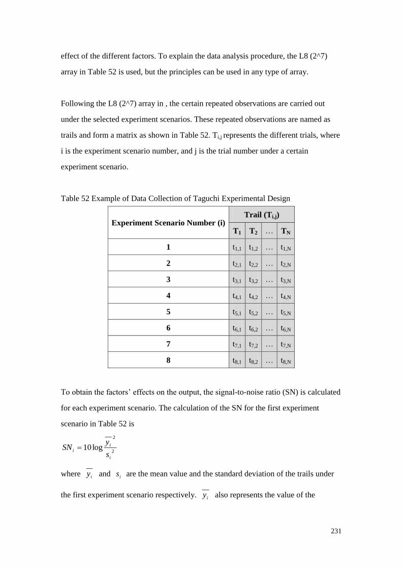
231

effect of the different factors. To explain the data analysis procedure, the L8 (2^7)

array in Table 52 is used, but the principles can be used in any type of array.

Following the L8 (2^7) array in , the certain repeated observations are carried out

under the selected experiment scenarios. These repeated observations are named as

trails and form a matrix as shown in Table 52. Ti,j represents the different trials, where

i is the experiment scenario number, and j is the trial number under a certain

experiment scenario.

Table 52 Example of Data Collection of Taguchi Experimental Design

Experiment Scenario Number (i) Trail (Ti,j)

T1 T2 … TN

1 t1,1 t1,2 … t1,N

2 t2,1 t2,2 … t2,N

3 t3,1 t3,2 … t3,N

4 t4,1 t4,2 … t4,N

5 t5,1 t5,2 … t5,N

6 t6,1 t6,2 … t6,N

7 t7,1 t7,2 … t7,N

8 t8,1 t8,2 … t8,N

To obtain the factors’ effects on the output, the signal-to-noise ratio (SN) is calculated

for each experiment scenario. The calculation of the SN for the first experiment

scenario in Table 52 is

2

2

log10i

ii

s

ySN

where iy and is are the mean value and the standard deviation of the trails under

the first experiment scenario respectively. iy also represents the value of the

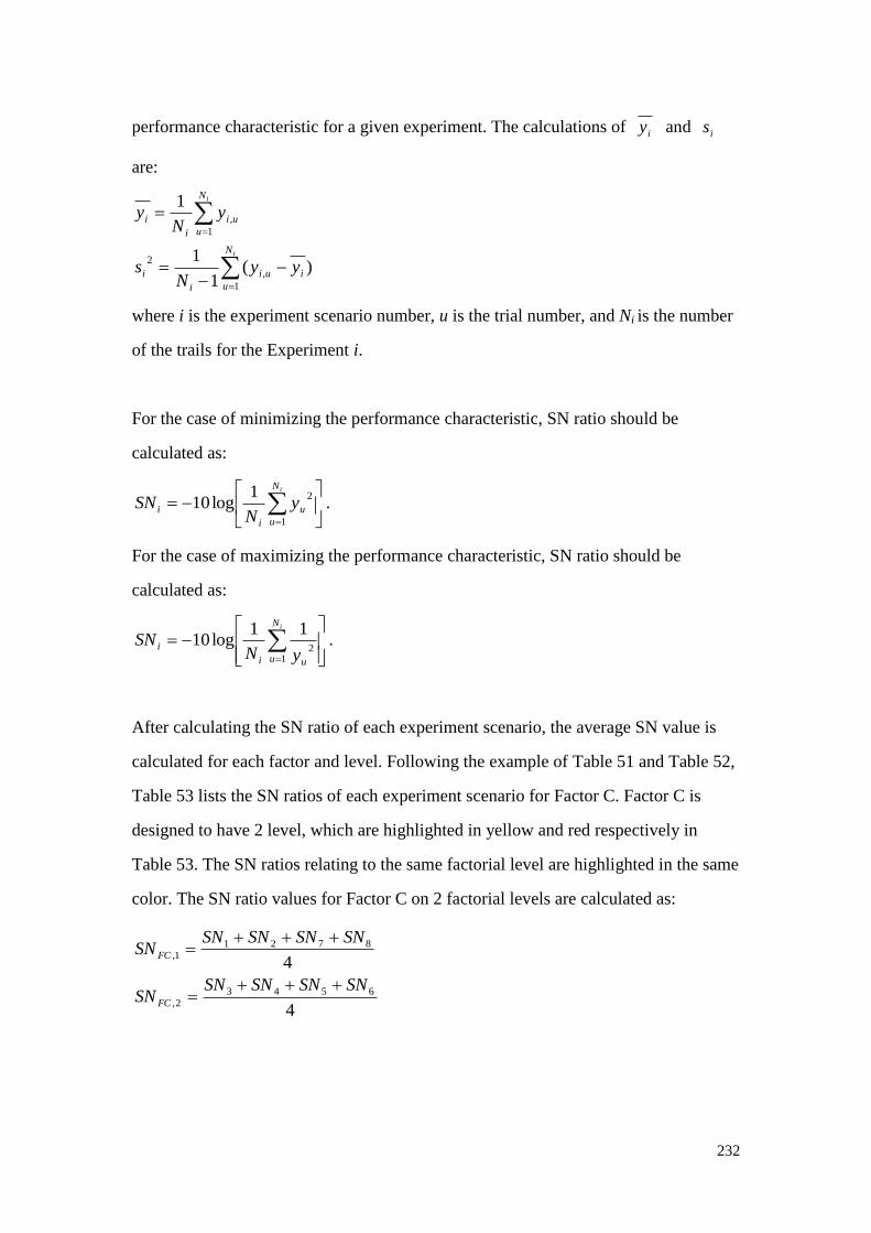
232

performance characteristic for a given experiment. The calculations of iy and is

are:

i

i

N

u

iui

i

i

N

u

ui

i

i

yyN

s

yN

y

1

,

2

1

,

)(1

1

1

where i is the experiment scenario number, u is the trial number, and Ni is the number

of the trails for the Experiment i.

For the case of minimizing the performance characteristic, SN ratio should be

calculated as:

iN

u

u

i

i yN

SN1

21log10 .

For the case of maximizing the performance characteristic, SN ratio should be

calculated as:

iN

u ui

iyN

SN1

2

11log10 .

After calculating the SN ratio of each experiment scenario, the average SN value is

calculated for each factor and level. Following the example of Table 51 and Table 52,

Table 53 lists the SN ratios of each experiment scenario for Factor C. Factor C is

designed to have 2 level, which are highlighted in yellow and red respectively in

Table 53. The SN ratios relating to the same factorial level are highlighted in the same

color. The SN ratio values for Factor C on 2 factorial levels are calculated as:

4

4

6543

2,

8721

1,

SNSNSNSNSN

SNSNSNSNSN

FC

FC

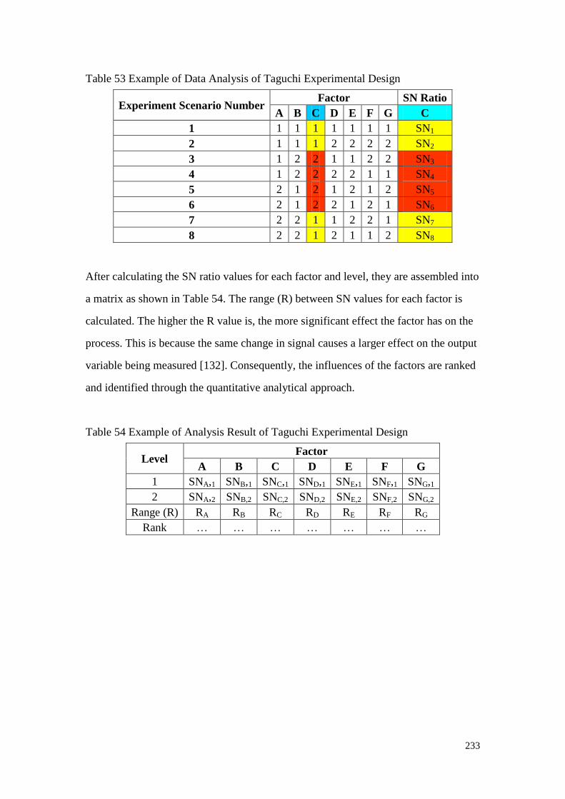
233

Table 53 Example of Data Analysis of Taguchi Experimental Design

Experiment Scenario Number Factor SN Ratio

A B C D E F G C

1 1 1 1 1 1 1 1 SN1

2 1 1 1 2 2 2 2 SN2

3 1 2 2 1 1 2 2 SN3

4 1 2 2 2 2 1 1 SN4

5 2 1 2 1 2 1 2 SN5

6 2 1 2 2 1 2 1 SN6

7 2 2 1 1 2 2 1 SN7

8 2 2 1 2 1 1 2 SN8

After calculating the SN ratio values for each factor and level, they are assembled into

a matrix as shown in Table 54. The range (R) between SN values for each factor is

calculated. The higher the R value is, the more significant effect the factor has on the

process. This is because the same change in signal causes a larger effect on the output

variable being measured [132]. Consequently, the influences of the factors are ranked

and identified through the quantitative analytical approach.

Table 54 Example of Analysis Result of Taguchi Experimental Design

Level Factor

A B C D E F G

1 SNA,1 SNB,1 SNC,1 SND,1 SNE,1 SNF,1 SNG,1

2 SNA,2 SNB,2 SNC,2 SND,2 SNE,2 SNF,2 SNG,2

Range (R) RA RB RC RD RE RF RG

Rank … … … … … … …

234

Appendix C. Data Collection Sheet to record the digital and

physical measurement results

235

Measurement scenarios Diameter result (m) Cylindricity result (m)

Probe

specification

Number of

probing points

Distribution of

probing points

Part

location

Mean

error

Standard

deviation Uncertainty

Mean

error

Standard

deviation

Uncertainty

1pt3D_22Z 4 120 Corner

1pt3D_22Z 4 120 Corner

1pt3D_22Z 4 120 Corner

1pt3D_22Z 9 240 Middle

1pt3D_22Z 9 240 Middle

1pt3D_22Z 9 240 Middle

1pt3D_22Z 15 360 Centre

1pt3D_22Z 15 360 Centre

1pt3D_22Z 15 360 Centre

3D_78Z 4 240 Centre

3D_78Z 4 240 Centre

3D_78Z 4 240 Centre

3D_78Z 9 360 Corner

3D_78Z 9 360 Corner

3D_78Z 9 360 Corner

3D_78Z 15 120 Middle

3D_78Z 15 120 Middle

3D_78Z 15 120 Middle

5D_40Z 4 360 Middle

5D_40Z 4 360 Middle

5D_40Z 4 360 Middle

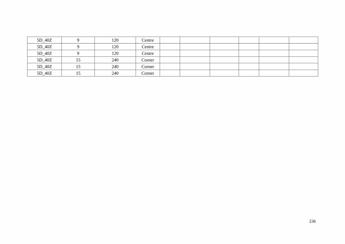
236

5D_40Z 9 120 Centre

5D_40Z 9 120 Centre

5D_40Z 9 120 Centre

5D_40Z 15 240 Corner

5D_40Z 15 240 Corner

5D_40Z 15 240 Corner

237

Reference

1 Wikipedia, 2008, Dimensional metrology [online]. Wikipedia. Available at:

https://en.wikipedia.org/wiki/Dimensional_metrology [Accessed 28 May 2013].

2 Tang, X. Q. and Yun H., 2008. Data model for quality in product lifecycle.

Computers in industry, 59 (2-3), pp.167-179.

3 Maropoulos, P., Guo, Y., Jamshidi, J. and Cai, B., 2008. Large Volume Metrology

Process Models: A framework for integrating measurement with assembly planning.

CIRP Annals - Manufacturing Technology, 57(1), pp.477–480.

4 Van Gestel, N., 2011. Determining measurement uncertainties of feature

measurements on CMMs. Thesis (PhD). Katholieke Universiteit Leuven, Belgium.

5 Llewellyn, J., 2013. Introduction: Measurement good practice in the supply chain

[Online]. BMTA: British Measurement and Testing Association. Available at:

https://connect.innovateuk.org/c/document_library/get_file?p_l_id=10355645&fold

erId=11590307&name=DLFE-137688.pdf [Accessed 28 May2013].

6 Bamforth, P., 2013. Product verification and its value for the aerospace industry

[Industrial presentation]. Rolls-Royce Plc [presented on Tue 19/03/2013].

7 Kruth, J. P., Bartscher, M., Carmignato, S., Schmitt, R., De Chiffre, L. and

Weckenmann, A., 2011. Computed tomography for dimensional metrology. CIRP

Annals - Manufacturing Technology, 60 (2), pp. 821–842.

8 Shen, W., Wang and L., Hao, Q., 2006. Agent-based distributed manufacturing

process planning and scheduling: a state-of-the-art survey. IEEE Transactions on

Systems, Man and Cybernetics—Part C: Applications and Reviews, 36 (4), pp.

563–577

9 Kimura, F., 1993. Product and process modelling as a kernel for virtual

manufacturing environment. CIRP Annals - Manufacturing Technology, 42(1), pp.

147–151.

238

10 Baxter, D., Gao, J., Case, K, Harding, J., Young, B., Cochrane, S. and Dani, S.,

2007. An engineering design knowledge reuse methodology using process

modelling. Research in Engineering Design, 18(1), pp. 37–48.

11 Zhao, Y., Kramer, T., Stone, R., Hoffman, M., Hoffman, S. and Rippey, W., 2012.

Design and usage guide for version 0.92 of the Quality Information Framework

data model and XML (Extensible Markup Language) Schemas. Washington:

National Institute of Standards and Technology (NIST).

12 Balsamo, A., Di Ciommo, M., Mugno, R., Rebaglia, B.I., Ricci, E. and Grella, R.,

1999. Evaluation of CMM uncertainty through Monte Carlo simulations. CIRP

Annals - Manufacturing Technology, 48(1), pp. 425–8.

13 Wilhelm, R.G., Hocken, R. and Schwenke, H., 2001. Task specific uncertainty in

coordinate measurement, CIRP Annals - Manufacturing Technology, 50 (2), pp.

553–563.

14 Summerhaysa, K., Henkea, M., Brownb, C., Henke, R. and Baldwin, J., 2002. A

tool for determining task-specific measurement uncertainties in GD&T

parameters obtained from coordinate measuring machines [online]. USA:

MetroSage LLC and Honeywell Inc. Available from:

http://www.aspe.net/publications/Annual_2002/PDF/PAPERS/4stdmet/911.PDF

[accessed 12 March 2013].

15 Baldwin, J., Summerhays, K., Campbell, D. and Henke, R., 2007. Application of

simulation software to coordinate measurement uncertainty evaluations. Measure,

2 (4), pp. 40–52.

16 Arenhart, F., Donatelli, G. and Porath, M., 2012. An experimental method for

assessing the contribution of the production process variations to the task-specific

uncertainty of coordinate measurements. Measurement, 45(3), pp. 507–516.

17 Maropoulos, P.G. and Ceglarek, D., 2010. Design verification and validation in

product lifecycle. CIRP Annals - Manufacturing Technology, 59(2), pp. 740-759.

18 Zhao, Y. F., Kramer, T., Rippey, W., Horst, J. and Proctor, F., 2012. An integrated

data model for quality information exchange in manufacturing systems.

239

Proceedings of the 37th MATADOR Conference, 25-27 July 2012 Manchester,

Manchester: University of Manchester, pp. 5-9.

19 Bell, S., 1999. Measurement good practice guide No. 118: a beginner’s guide to

uncertainty of measurement, 2nd

ed. Teddington, UK: National Physical

Laboratory.

20 JCGM 200:2008. International vocabulary of basic and general terms in

metrology (VIM), 3rd edition. International Organisation for standardisation

(ISO).

21 JCGM 100:2008. Evaluation of measurement data — Guide to the expression of

uncertainty in measurement (GUM). International Organisation for standardisation

(ISO).

22 Phillips, S., Borchardt, B. and Abackerli, A., 2003. The Validation of CMM Task

Specific Measurement Uncertainty Software. Proceedings of the ASPE 2003

summer topical meeting “Coordinate Measuring Machines”, June 25 –26 2003

North Carolina, USA. USA: American Society for Precision Engineering (ASPE),

pp. 1-6.

23 Forbes, A.B., 2006. Measurement uncertainty and optimised conformance

assessment. Measurement, 39 (9), pp. 808–814.

24 Pendrill, L.R., 2008. Operating ‘cost’ characteristics in sampling by variable and

attribute. Accreditation and Quality Assurance, 13(11), pp 619-631.

25 Baldwin, J.M., Summerhays, K.D. and Campbell, D.A., 2010. Evaluating the

Economic Impact of CMM Measurement Uncertainty. Proceedings of

Measurement Science Conference, Pasadena, USA.

26 JCGM 104:2009. Evaluation of measurement data – An introduction to the

"Guide to the expression of uncertainty in measurement" and related documents.

International Organisation for standardisation (ISO).

27 JCGM 101:2008. Evaluation of measurement data – Supplement 1 to the "Guide

to the expression of uncertainty in measurement" – Propagation of distributions

using a Monte Carlo method. International Organisation for standardisation (ISO).

240

28 John, H., Lehman, C., Wang, M., Dowell, L.M. and Hadler, J.A., 2009.

Uncertainty calculation for spectral-responsivity measurements. Journal of

Research of the National Institute of Standards and Technology, 114(5), pp.

287-291..

29 Oliveira, S.P., Rocha, A.C., Filho, T.J. and Couto P.R.G., 2008. Uncertainty of

measurement by Monte-Carlo simulation and metrological reliability in the

evaluation of electric variables of PEMFC and SOFC fuel cells. Measurement,

42(10), pp.1497-1501.

30 Müller, M. andRink, C., 2009. On the convergence of the Monte Carlo block

design. Metrologia, 46(5), pp. 404-408.

31 Ellison, S.L.R., 1998. Using validation data for ISO measurement uncertainty

estimation - Part 1. Principles of an approach using cause and effect analysis. The

Analyst, 123(6), pp. 1387-1392.

32 Bich, W., Cox, M. G. and Harris, P. M., 2006. Evolution of the Guide to the

Expression of Uncertainty in measurement. Metrologia, 43(4), pp. S161–S166.

33 Cox, M. and Harris, P., 2003. The GUM and its planned supplemental guides.

Accreditation and Quality Assurance, 8(7-8), pp. 375-379.

34 Ridler, N., Lee, B., Martens, J. and Wong, K., 2007. Measurement uncertainty,

traceability, and the GUM. IEEE Microwave Magazine, 8(4), pp. 44-53.

35 Krulikowski, A., 1997. Fundamentals of geometric dimensioning and tolerancing.

2nd

ed. New York: Delmar Cengage Learning.

36 ASME Y14.5M: 1994. Dimensioning and Tolerancing. American Society of

Mechanical Engineers (ASME).

37 Shah, J. J., Ameta, G., Shen, Z. and Davidson, J., 2007. Navigating the tolerance

analysis maze. Computer-Aided Design & Applications, 4(5), pp.705-718.

38 Tsai, J.C. and Cutkosky, M.R., 1997. Representation and reasoning of geometric

tolerances in design. Artificial Intelligence for Engineering Design Analysis and

Manufacturing, 11(4), pp.325-341.

241

39 Chiabert, P., Lombardi, F. and Orlando, M., 1998. Benefits of geometric

dimensioning and tolerancing. Journal of Materials Processing Technology,

78(1-3), pp.29-35.

40 Shah, J.J., Yan, Y. and Zhang, B.C., 1998. Dimension and tolerance modeling and

transformations in feature based design and manufacturing. Journal of Intelligent

Manufacturing, 9(5), pp.475-488.

41 Zhang, Y., Hu, W. and Rong, Y., 2001. Graph-based set-up planning and

tolerance decomposition for computer-aided fixture design. International Journal

of Production Research, 39(14), pp.3109-3126.

42 Shen, Z.S., Shah, J.J. and Davidson, J.K., 2008. Analysis neutral data structure for

GD&T. Journal of Intelligent Manufacturing, 19(4), pp.455–472.

43 Kong, Z., Huang, W. and Oztekin, A., 2009. Variation propagation analysis for

multistation assembly process with consideration of GD&T factors. Journal of

Manufacturing Science and Engineering, 131(5), pp. 051010-1-10.

44 Hunter, R., Perez, J., Marquez, J. and Hernandez, J.C., 2007. Modelling the

integration between technological product specifications and inspection process.

Journal of Materials Processing Technology, 91(1-3), pp.34-38.

45 Mohib, A., Azab, A. and ElMaraghy, H., 2009. Feature-based hybrid inspection

planning: A mathematical programming approach. International journal of

computer integrated manufacturing, 22(1), pp.13-29.

46 Prieto, F., Boulanger, P., Lepage, R. and Redarce, T., 2002. Automated inspection

system using range data. Proceedings of IEEE International Conference

on Robotics and Automation, 3, pp.2557-2562.

47 Prieto, F., Redarce, T., Lepage, R. and Boulanger P., 2002. An automated

inspection system. International Journal of Advanced Manufacturing Technology,

Issue 19, pp. 917–925.

48 Son, S., Park, H. and Lee, K. H., 2002. Automated laser scanning system for

reverse engineering and inspection. International Journal of Machine Tools

Manufacturing, Issue 2, pp.889–897.

242

49 Gao, J., Gindy N., and Chen, X., 2006. An automated GD&T inspection system

based on non-contact 3D digitization. International Journal of Production

Research, 44(1), pp.117.

50 Rennels, K.E., 2003. Current methodologies for geometric dimensioning and

tolerancing. Proceedings of the Electrical Insulation Conference and Electrical

Manufacturing & Coil Winding Technology Conference, 23-25 September 2003,

pp.565–569.

51 Watts, D., 2007. The ‘‘GD&T Knowledge Gap’’ in Industry. Proceedings of the

ASME International Design Engineering Technical Conferences, 4th

-7th

September 2007 Las Vegas, NV, USA. New York: ASME, pp. 597–604.

52 Zhang, Y. and Yang, M., 2009. A coordinate SPC model for assuring designated

fit quality via quality-oriented statistical tolerancing. Computers and Industrial

Engineering, 57(1), pp.73–79.

53 BS 8888:2008. Technical Product Specification – Specification. British Standard

Institution (BSI)..

54 Henzold, G., 2006. Geometrical Dimensioning and Tolerancing for Design,

Manufacturing and Inspection. In A Handbook for Geometrical Product

Specification using ISO and ASME standards. 2nd

ed. London:

Butterworth-Heinemann, Page(s): 372 – 373.

55 ISO/TS 17450-1:2011. Geometrical product specifications (GPS) – General

concepts -- Part 1: Model for geometrical specification and verification.

International Organisation for standardisation (ISO).

56 ISO/TS 17450-2:2002. Geometrical product specifications (GPS) – General

concepts -- Part 2: Basic tenets, specifications, operators and uncertainties.

International Organisation for standardisation (ISO).

57 Nielsen, H.S., 2003. Specifications, operators and uncertainties. Proceedings of

the 8th CIRP International Seminar on Computer Aided Tolerancing, April 2003

Charlotte, NC, USA.

243

58 Lu, W., Jiang, X., Scott, P.J. and Lan, X., 2009. A host system for form tolerance

specification in the next-generation GPS based on AutoCAD. Proceedings of he

11th CIRP Conference on Computer Aided Tolerancing -“Geometric Variations

within Product Life-Cycle Management”, 26th

-27th

March 2009 Annecy, France.

59 Dantan, J., Bruyere, J., Baudouin, C. and Mathieu, L., 2007. Geometrical

Specification Model for Gear-Expression, Metrology and Analysis. CIRP

Annals-Manufacturing Technology, 56(1), pp.517-520.

60 N Nielsen, H.S., 2006. New concepts in specifications, operators and uncertainties

and their impact on measurement and instrumentation. Measurement Science

Technology, 17(3), pp.541–544.

61 ISO 10360-2:2002. Geometrical Product Specifications (GPS) - Acceptance and

Reverification Tests for Coordinate Measuring Machines (CMM) - Part 2: CMMs

used for measuring size. British Standard Institution (BSI).

62 ISO 10360-5:2010. Geometrical Product Specifications (GPS) - Acceptance and

Reverification Tests for Coordinate Measuring Machines (CMM) - Part 5:

CMMs using single and multiple stylus contacting probing systems. British

Standard Institution (BSI).

63 Schwenke, H., Wäldele, F. and Wendt, K., 1998. Abnahme, Überwachung und

Kalibrierung von flexiblen Industriemeßsystemen mit CCD-Kameras.

Braunschweig, Germany: Physikalisch-Technische Bundesanstalt (PTB).

64 Luhmann, T. and Wendt, K., 2000. Recommendations for an acceptance and

verification test of optical 3-D measurement systems. International Archives for

Photogrammetry and Remote Sensing, 33(5) pp.493-499.

65 Keferstein, C. P. and Züst, R., 2004. Minimizing technical and financial risk when

integrating and applying optical sensors for in-process measurement. International

Intelligent Manufacturing Systems Forum, Italia, Vol. 17, pp. 475-482.

66 Pumm, C. and Präzision, W., 2005. New ISO standards. ia.cmm International

Conference, Germany, April 28th, 2005.

244

67 ISO/TS 15530-4: 2000. GPS – CMM: Techniques for evaluation of uncertainty of

measurement - Part 4: Evaluating task-specific measurement uncertainty using

simulation. International Organisation for standardisation (ISO).

68 Zhao, F., Xu, X. and Xie, S.Q., 2009. Computer-aided Inspection Planning – The

State of the Art. Computers in Industry, 60(7), pp.453–466.

69 Cho, M.W., Lee, H., Yoon, G.S. and Choi, J., 2005. A feature-based inspection

planning system for coordinate measuring machines. The International Journal of

Advanced Manufacturing Technology, 26(9-10), pp.1078–1087.

70 Lin, Y.J., Mahabaleshwarkar, R. and Massina, E., 2001. CAD-based CMM

Dimensional Inspection Path Planning: A Generic Algorithm. Robotica, 19(2),

pp.137–148.

71 Lee, G., Mou, J. and Shen, Y., 1997. Sampling strategy design for dimensional

measurement of geometric features using coordinate measuring machine.

International Journal of Machine Tools and Manufacture, 37(7), pp.917–934.

72 Zhang, S.G., Ajmal, A., Wootton, J. and Chisholm, A., 2000. A feature-based

inspection process planning system for coordinate measuring machine. Journal of

Materials Processing Technology, 107(1-3), pp.111–118.

73 Limaiem, A. and ElMaraghy, H.A., 1999. CATIP: a computer-aided tactile

inspection planning system. International Journal of Production Research, 37(2),

pp.447–465.

74 Hwang, Y., Tsai, C.Y., and Chang, C.A., 2004. Efficient inspection planning for

coordinate measuring machines. International Journal of Manufacturing

Technology, 23(9-10), pp.732–742.

75 Wong, F.S.Y., Chuah, K.B. andVenuvinod, P.K., 2006. Automated inspection

process planning: algorithmic inspection feature recognition, and case

representation for CBR. Robotics and Computer-Integrated Manufacturing, 22(1),

pp.56–68.

245

76 Lee, H., Cho, M.W., Yoon, G.S. and Choi, J.H., 2004. A computer-aided

inspection planning system for online measurement-Part I: Global inspection

planning. KSME International Journal, 18 (8), pp.1349–1357.

77 Chung, S.C., 1999. CAD/CAM integration of on-the-machine measuring and

inspection system for free-formed surfaces. Proceedings of American Society for

Precision Engineering, 20, pp. 267–270.

78 Cho, M.-W. and Seo, T.-L., 2002. Inspection planning strategy for the online

measurement process based on CAD/CAM/CAI integration. International Journal

of Manufacturing Technology, 19 (8), pp. 607–617.

79 Vafaeesefat, A. and EIMaraghy, G.A., 2000. Automated accessibility analysis and

measurement clustering for CMMs. International Journal of Production Research,

38(10), pp.2215–2231.

80 Lu, C.G., Morton, D., Wu, M.H. andMyler, P., 1999. Genetic algorithm modelling

and solution of inspection path planning on a coordinate measuring machine. The

International Journal of Advanced Manufacturing Technology, 15(6),

pp.409–416.

81 Huang, H.L. and Ha, S., 2002. Hybrid Neuro-fuzzy approach to the generation of

measuring points for knowledge-based inspection planning. International Journal

of Production Research, 40(11), pp.2507-2520.

82 Cho, M.-W., Lee, H., Yoon, G.-S. and Choi, J.-H., 2004. A computer-aided

inspection planning system for online measurement-Part II: Local inspection

planning. KSME International Journal, 18, pp.1358–1367.

83 Woo, T. and Liang, R., 1993. Optimal sampling for coordinate measurement: its

definition and algorithm. Quality through Engineering Design, 16, pp. 333–346.

84 Dowling, M.M., Griffin, P.M., Tsui, K.-L. and Zhou, C., 1997. Statistical issues in

geometric feature inspection using coordinate measuring machines. Technometrics,

39(1), pp.3–17.

246

85 Jiang, B.C. and Chiu, S.D., 2002. Form tolerance-based measurement points

determination with CMM. Journal of Intelligent Manufacturing, 13(2),

pp.101–108.

86 Elkott, F., ElMaraghy, H.A. and Elmaraghy, W.H., (2002). Automatic sampling

for CMM inspection planning of free-form surfaces. International Journal of

Production Research, 40(11), pp.2653–2676.

87 Moroni, G., Polini, and W., Rasella, M., 2003. Manufacturing Signatures and

CMM Sampling Strategies [online]. Available from:

http://www.aspe.net/publications/Summer_2003/03SU%20Extended%20Abstract

s/Moroni.PDF [accessed 13 July 2012].

88 Cui, C., Fu, S. and Huang, F, 2009. Research on the uncertainties from different

form error evaluation methods by CMM sampling. The International Journal of

Advanced Manufacturing Technology, 43(1-2), pp.136-145.

89 Liu, Q., Zhang, C.C. and Wang, H.P.B., 2001. On the effects of CMM

measurement error on form tolerance estimation. Measurement, 30(1), pp.33–47.

90 Odayappan, O., Raja, J., Hocken, R.J. and Chen, K., 1993. Sampling strategies for

circles in coordinate measuring machines. Proceedings of the American Society of

Precision Engineering, 8, pp. 70–72.

91 Dhanish, P.B. and Mathew, J., 2006. Effect of CMM point coordinate uncertainty

on uncertainties in determination of circular features. Measurement, 39(6),

pp.522–531.

92 Chan, F.M.M., King, T.G. andStout, K.J., 1996. The influence of sampling

strategy on a circular feature in coordinate measurements. Measurement, 19(2),

pp.73–81.

93 Elkott, D.F., Elmaraghy, H.A. and Elmaraghy, W.H., 2002. Automatic sampling

for CMM inspection planning of free-form surfaces. International Journal of

Production Research, 40(11) , pp.2653-2676.

247

94 Barini, E. M., Tosello, G. and De Chiffre, L., 2007. Uncertainty analysis of

point-by-point sampling complex surfaces using touch probe CMMs: DOE for

complex surfaces verification with CMM. Precision Engineering, 34(1), pp.16-21.

95 Lu, E., Ni, J. and Wu, S. M., 1994. An algorithm for the generation of an optimum

CMM inspection path. ASME Journal of Dynamic Systems, Measurements, and

Control, 116, pp.396-404.

96 Albuquerque, V.A., Liou, F.W. and Mitchell, O.R., 2000. Inspection point

placement and path planning algorithms for automatic CMM inspection.

International Journal of Computer Integrated Manufacturing, 13(2), pp.107–120.

97 Ainsworth, I., Ristic, M. and Brujic, D., 2000. CAD-based measurement path

planning for free-form shapes using contact probes. International Journal of

Advanced Manufacturing Technology,16 (1), pp.23–31.

98 Lin, Y.J. and Murugappan, P., 1998. A new algorithm for CAD-directed CMM

dimensional inspection. International Journal of Advanced Manufacturing

Technology, 16 (2), pp. 107–112.

99 Yu, D., Li, X.J., Xiong, Y. and Gao Z.H., 2010. Reconstructing of Prototype

Surface with Reverse Engineering and Data Process Technology. Key Engineering

Materials, 458, pp. 368-373.

100 Javidrad, F. and Rahmati, R., 2009. An integrated re-engineering plan for the

manufacturing of aerospace components. Materials & Design, 30(5),

pp.1524–1532.

101 Chang, D.Y. and Chang, Y.M., 2002. A freeform surface modelling system

based on laser scan data for Reverse Engineering. The International Journal of

Advanced Manufacturing Technology, 20(1), pp9-19.

102 Zhang, Y., 2003. Research into the engineering application of reverse

engineering technology. Journal of Materials Processing Technology, 139(1–3),

pp.472–4755.

248

103 Zhang, Y., Fan, Y. and Chu, X., 1999. Principle and key technologies of reverse

engineering. Journal of Kunming University Science and Technology, 24(4), pp.

42–46.

104 Rajamohan, G., Shunmugam, M.S., Samuel, G.L., 2011. Effect of probe size and

measurement strategies on freeform profile deviations using coordinate measuring

machine. Measurement, 44(5), 832-841.

105 Tosello, G., Hansen, H.N. and Gasparin, S., 2009. Applications of Dimensional

Micro Metrology to the Product and Process Quality Control in Manufacturing of

Precision Polymer Micro Components. CIRP Annals – Manufacturing Technology,

58(1), pp. 467–472.

106 Fleischer, J., Lanza, G. and Schlipf, M., 2008. Statistical Quality Control in

Micro-manufacturing Through Multivariate μ-EWMA Chart. CIRP Annals –

Manufacturing Technology, 57(1), pp.521–524.

107 Kunzmann, H., Pfeifer, T., Schmitt, R., Schwenke, H. and Weckenmann, A.,

2005. Productive Metrology—Adding Value to Manufacture, CIRP Annals –

Manufacturing Technology, 54 (2), pp.691–713.

108 Pendrill, L.R., 2010. Optimised uncertainty and cost operating characteristics:

new tools for conformity assessment - Application to geometrical product control

in automobile industry. International Journal of Metrology and Quality

Engineering, 1(02), pp.105-110.

109 Henke, R.P., Summerhays, K.D., Baldwin, J.M., Cassou, R.M. and Brown, C.W.,

1999. Methods for evaluation of systematic geometric deviations in machined

parts and their relation to process variables. Precision Engineering, 23(4),

pp.273–292.

110 Takamasu, K., 2011. Present problems in coordinate metrology for nano and

micro scale measurements, Mapan, 26(1) pp.3-14.

111 Trapet, E. and Waldele, F., 1996. The virtual CMM concept. In: Advanced

Mathematical Tools in Metrology II. Singapore: World Scientific Publishing

Company, pp.238–247.

249

112 Phillips, S.D., Borchardt, B.R., Sawyer, D., Estler, W.T., Ward, D., Eberhardt,

K., and Levenson, M. S., 1997. The Calculation of CMM Measurement

Uncertainty via the Method of Simulation by Constraints. American Society for

Precision Engineering, 16, pp.443-446.

113 Haitjema, H., Van Dorp, B., Morel, M. and Schellekens, P.H.J., 2001.

Uncertainty estimation by the concept of virtual instruments. Proceedings of SPIE

- Recent Developments in Traceable Dimensional Measurements, 18th June 2001

Munich, Germany.

114 Trenk M., Franke, M. and Schwenke, H., 2004. The “Virtual CMM” a software

tool for uncertainty evaluation – practical application in an accredited calibration

lab. ASPE Proceedings on Uncertainty Analysis in Measurement and Design, pp.

1-6.

115 Takamasu, K., 2002. Final Research Report - International Standard

Development of Virtual CMM (Coordinate Measuring Machine). Tokyo: New

Energy and Industrial Technology Development Organization (NEDO).

116 Forbes, A.B. and Harris, P.M., 2000. Simulated Instruments and Uncertainty

Estimation. London: National Physical Laboratory (CMSC 01/00).

117 Pahk, H.J., Burdekin, M. and G N Peggs, 1998. Development of virtual

coordinate measuring machines incorporating probe errors. Proceedings of the

Institution of Mechanical Engineers, Part B: Journal of Engineering

Manufacture, 212(7), pp.533-548.

118 Hu, Y., Yang, Q. and Wei P., 2009. Development of A Novel Virtual Coordinate

Measuring Machine. Proceedings of MTC 2009 - International Instrumentation

and Measurement Technology Conference, 5th

-7th

May 2009 Singapore. New

York: IEEE, pp.230-233.

119 Zhang, G., Veale, R., Charlton, T., Borchardt, B. and Hocken, R., 1985. Error

compensation of coordinate measuring machines. CIRP Annals - Manufacturing

Technology, 34(1), pp.445–448.

250

120 Barakat, N.A., Elbestawi, M.A. and Spence, A.D., 2000. Kinematic and

geometric error compensation of a coordinate measuring machine. International

Journal of Machine Tools & Manufacture, 40(6), pp.833–850.

121 Van Dorp, B., Haitjema, H., Delbressine, F., Bergmans, R., and Schellekens, P.,

2001. A virtual CMM using Monte Carlo methods based on frequency content of

the error signal. Proceedings of SPIE, vol. 4401, pp. 58-167.

122 van Dorp, B., Delbressine, F., Haitjema, H., and Schellekens, P., 2001,

Calculation of measurement uncertainty for multi-dimensional machines using the

method of surrogate data. In: Advanced Methematical and Computational Tools in

Metrology. Singapore: World Scientific Publishing Company, pp. 344-351.

123 ANSI/ASME B89.4.1:1997. Methods for Performance Evaluation of Coordinate

Measuring Machines. ASME.

124 Beaman, J. and Morse, E., 2010. Experimental evaluation of software estimates

of task specific measurement uncertainty for CMMs. Precision Engineering, 34(1),

pp.28–3.

125 Salsbury, J.G., 1995. A Simplified Methodology for the Uncertainty Analysis of

CMM Measurements. Indianapolis, USA: Society of Manufacturing Engineers,

(IQ95-155:1–22).

126 Phillips, S.D., Borchardt, B., Estler, W.T. and Buttress J., 1998. The estimation

of measurement uncertainty of small circular features measured by coordinate

measuring machines. Precision Engineering, 22(2), pp.87-97.

127 Abackerli, A.J., Pereira, P.H. and Calônego, N., 2010. A case study on testing

CMM uncertainty simulation software (VCMM). Journal of the Brazilian Society

of Mechanical Sciences and Engineering, 32(1), pp.8-14.

128 Guo, Y., 2006. Integrated process planning and scheduling for common

prismatic parts in a 5-axis CNC environment. Thesis (PhD), University of Bath,

Bath, UK.

251

129 Blockley, D.I. and Henderson, J. R., 1980. Structural failures and the growth of

engineering knowledge. ICE Proceedings, 70(3), pp.567 –579

130 Mebrahtu H., Walker R. and Mileham T., 2005. Manufacturing simulation

optimization: an expert mechanism approach. Proceedings of the Institution of

Mechanical Engineers, Part B: Journal of Engineering Manufacture, 223(12),

pp.1625-1634.

131 Metrosage, 2003. PUNDIT/CMM User Manual. California, USA: MetroSage

LLC.

132 Taguchi, G., Konishi, S. and Konishi S., 1987. Methods, Orthogonal Arrays

and Linear Graphs Tools for Quality Engineering. USA: American Supplier

Institute.

133 Wikipedia, 2012. SolidWorks [online]. Wikipedia. Available from:

http://en.wikipedia.org/wiki/SolidWorks [accessed on 03/03/2013].

134 Flack, D., 2001. Measurement Good Practice Guide No. 41: CMM measurement

strategies. London: National Physical Laboratory (NPL).

135 Flack, D., 2001. Measurement Good Practice Guide No. 41: CMM measurement

strategies. London: National Physical Laboratory (NPL).

136 Lindqvist, R., 2011. Geometrical and dimensional Measurement Planning: - a

systematic and holistic approach. Thesis (PhD). The Royal Institute of

Technology, Stockholm, Denmark.