www.iap.uni-jena.de

Metrology and Sensing

Lecture 13: Metrology of aspheres and freeforms

2018-01-25

Herbert Gross

Winter term 2017

2

Preliminary Schedule

No Date Subject Detailed Content

1 19.10. Introduction Introduction, optical measurements, shape measurements, errors,

definition of the meter, sampling theorem

2 26.10. Wave optics Basics, polarization, wave aberrations, PSF, OTF

3 02.11. Sensors Introduction, basic properties, CCDs, filtering, noise

4 09.11. Fringe projection Moire principle, illumination coding, fringe projection, deflectometry

5 16.11. Interferometry I Introduction, interference, types of interferometers, miscellaneous

6 23.11. Interferometry II Examples, interferogram interpretation, fringe evaluation methods

7 30.11. Wavefront sensors Hartmann-Shack WFS, Hartmann method, miscellaneous methods

8 07.12. Geometrical methods Tactile measurement, photogrammetry, triangulation, time of flight,

Scheimpflug setup

9 14.12. Speckle methods Spatial and temporal coherence, speckle, properties, speckle metrology

10 21.12. Holography Introduction, holographic interferometry, applications, miscellaneous

11 11.01. Measurement of basic

system properties Bssic properties, knife edge, slit scan, MTF measurement

12 18.01. Phase retrieval Introduction, algorithms, practical aspects, accuracy

13 25.01. Metrology of aspheres

and freeforms Aspheres, null lens tests, CGH method, freeforms, metrology of freeforms

14 01.02. OCT Principle of OCT, tissue optics, Fourier domain OCT, miscellaneous

15 08.02. Confocal sensors Principle, resolution and PSF, microscopy, chromatical confocal method

3

Content

Aspheres

Null lens tests

CGH method

Freeforms

Metrology of freeforms

Asphere

Cylindrical lens

Freeform lens

Axicon

Prisms

4

Optical Components

Manufacturing of Freeform Surfaces

Ref: G. Günther

5

6

Manufacturing of Aspheres / Freeforms

Grinding / polishing

Molding(low TG glasses or plastics)

Ref: C. Menke

Diamond turning

Tooling machine

Fast server tool

7

Freeform Manufacturing

Ref: B. Satzer

Form of Material Removal

Ref: R. Börret

Traditional material removal:

surface / area contact

Diamond turning of freeforms:

pointlike contact

special deviation types with local errors

8

22 yxz

222

22

111 yxc

yxcz

22

22 yxRRRRz xxyy

Conic section

Special case spherical

Cone

Toroidal surface with

radii Rx and Ry in the two

section planes

Generalized onic section without

circular symmetry

Roof surface

2222

22

1111 ycxc

ycxcz

yyxx

yx

z y tan

9

Aspherical Surface Types

222

22

111 yxc

yxcz

1

2

b

a

2a

bc

1

1

cb

1

1

ca

Explicite surface equation, resolved to z

Parameters: curvature c = 1 / R

conic parameter

Influence of on the surface shape

Relations with axis lengths a,b of conic sections

Parameter Surface shape

= - 1 paraboloid

< - 1 hyperboloid

= 0 sphere

> 0 oblate ellipsoid (disc)

0 > > - 1 prolate ellipsoid (cigar )

10

Conic Sections

Simple Asphere – Parabolic Mirror

sR

yz

2

2

axis w = 0° field w = 2° field w = 4°

Equation

Radius of curvature in vertex: Rs

Perfect imaging on axis for object at infinity

Strong coma aberration for finite field angles

Applications:

1. Astronomical telescopes

2. Collector in illumination systems

Simple Asphere – Elliptical Mirror

22

2

)1(11 cy

ycz

F

s

s'

F'

Equation

Radius of curvature r in vertex, curvature c

eccentricity

Two different shapes: oblate / prolate

Perfect imaging on axis for finite object and image loaction

Different magnifications depending on

used part of the mirror

Applications:

Illumination systems

Spherical Aberration

Spherical aberration:

On axis, circular symmetry

Perfect focussing near axis: paraxial focus

Real marginal rays: shorter intersection length (for single positive lens)

Optimal image plane: circle of least rms value

paraxial

focus

marginal

ray focusplane of the

smallest

rms-value

medium

image

plane

As

plane of the

smallest

waist

2 A s

14

Aspherical Correction

Correction of spherical aberration by

an asphere

Ref: A. Herkommer

a) spherical

lens

b) aspherical

lens

refraction too

strong

asphere reduces

power

Perfect stigmatic imaging on axis:

Hyperoloid rear surface

Strong decrease of performance

for finite field size :

dominant coma

Alternative: ellipsoidal surface on front surface and concentric rear surface

Asphere: Perfect Imaging on Axis

1

1

1

1

1

2

2

2

2

n

ns

r

n

s

n

sz

ns

z

r

F

0

100

50

Dspot

w in °0 1 2

m]

Asphere far from pupil:

- ray bundels of field points

separated

- field dependend correction

- also impact on distortion

Asphere near pupil:

- all ray bundels equally affected

- problem field angles: coma

16

Impact of Asphere

surface 2

surface 15

Correction on axis and field point

Field correction: two aspheres

Aspherical Single Lens

spherical

one aspherical

double aspherical

axis field, tangential field, sagittal

250 m 250 m 250 m

250 m 250 m 250 m

250 m 250 m 250 m

a

a a

Reducing the Number of Lenses with Aspheres

Example photographic zoom lens

Equivalent performance

9 lenses reduced to 6 lenses

Overall length reduced

Ref: H. Zügge

436 nm

588 nm

656 nm

xpyp

DxDy

axis field 22°

xpyp

DxDy

xpyp

DxDy

axis field 22°

xpyp

DxDy

A1A3

A2

a) all spherical, 9 lenses

b) 3 aspheres, 6 lenses,

shorter, better performance

Photographic lens f = 53 mm , F# = 6.5

Lithographic Projection: Improvement by Aspheres

Considerable reduction

of length and diameter

by aspherical surfaces

Performance equivalent

2 lenses removable

a) NA = 0.8 spherical

b) NA = 0.8 , 8 aspherical surfaces

-13%-9%

31 lenses

29 lenses

Ref: W. Ulrich

Aspheres - Geometry

z

y

aspherical

contour

spherical

surface

z(y)

height

y

deviation

Dz

sphere

z

y

perpendicular

deviation Drs

deviation Dz

along axis

height

y

tangente

z(y)

aspherical

shape

Reference: deviation from sphere

Deviation Dz along axis

Better conditions: normal deviation Drs

Improvement by higher orders

Generation of high gradients

Aspherical Expansion Order

r

Dy(r)

0 0.2 0.4 0.6 0.8 1-100

-50

0

50

100

12. order

6. order

10. order8. order

14. order

2 4 6 8 10 12 1410

-1

100

101

102

103

order

kmax

Drms

[m]

Aspheres: Correction of Higher Order

Correction at discrete sampling

Large deviations between

sampling points

Larger oscillations for

higher orders

Better description:

slope,

defines ray bending

y y

residual spherical

transverse aberrations

Corrected

points

with

y' = 0

paraxial

range

y' = c dzA/dy

zA

perfect

correcting

surface

corrected points

residual angle

deviation

real asphere with

oscillations

points with

maximal angle

error

Polynomial Aspherical Surface

Standard rotational-symmetric description

0

0,5

1

1,5

2

0 0,2 0,4 0,6 0,8 1 1,2

h

h^4

h^6

h^8

h^10

h^12

h^14

h^16

M

m

m

mhahc

hhz

0

42

22

2

111)(

Ref: K. Uhlendorf

Basic form of a conic section superimposed by a Taylor expansion of z

h ... Radial distance to optical axis

... Curvature

c ... Conic constant

am ... Apherical coefficients

23

22 yxh

Forbes Aspheres

New representation of aspherical expansions according to Forbes (2007)

Special polynomials Qk(r2):

1. Contributions are orthogonal slope

2. tolerancing is easily measurable

3. optimization has better performance

4. usually fewer coefficients are necessary

5. use of normalized radial coordinate makes coefficients independent on diameter

Two different versions possible:

a) strong aspheres: deviation defined along z

b) mild aspheres: deviation defined perpendicular to the surface

24

max

2

2

22

2

)(111

)(k

k

kk rQarc

rcrz

25

Forbes Aspheres

Strong asphere Qcon Mild asphere Qbfs

sag along z-axis difference to best fit sphere

sag along local surface normal

not slope orthogonal slope orthogonal

true polynom not a polynomial

type Q 1 in Zemax type Q 0 in Zemax

direct tolerancing of coefficients no direct relation of coefficients to slope

max24 2

2 22

( ) ( )1 1 1

k

k k

k

c rz r r a Q r

c r

2

2 2

2 2

2

20

(r)1 1

1

1

M

m mc

m

crz

c r

r ra B r

c r

-1

-0,5

0

0,5

1

1,5

2

0 0,2 0,4 0,6 0,8 1 1,2

h

h^4*Q0

h^4*Q1

h^4*Q2

h^4*Q3

h^4*Q4

h^4*Q5

-0,5

0

0,5

0 0,2 0,4 0,6 0,8 1 1,2

h

u(1-u)B0

u(1-u)B1

u(1-u)B2

u(1-u)B3

u(1-u)B4

u(1-u)B5

Special correcting free shaped aspheres:

Inversion of incoming wave front

Application: final correction of lithographic systems

Aspheres – Correcting Residual Wave Aberrations

conventional lenslens with correcting

surface

Asphere :

The location of the center of curvature moves with the radial surface position

Conventional reflex light measurement in autocollimation is not possible

Curvature of Aspheres

aspherical surface

Cedge Czone Cinner

opticalaxis

moving center of curvature

Autocollimation Principle

Spherical test surface:

- incoming and outgoing wavefront spherical

- concentric waves around center of curvature:

autocollimation

Aspherical test surface

auxiliary lensspherical test

surface

center of

curvature

wavefronts

spherical

auxiliary lens

aspherical test

surface

incoming wavefront

spherical

outcoming wavefront

aspherical

paraxial

center of

curvature

Asphere Test with CGH

test-beam from/to

interferometer aspherical mirror CGH

Interferogram

without CGH:

with CGH:

to much interference fringes

analysis impossible

flat wave-front

simple analysis Ref: F. Burmeister

30

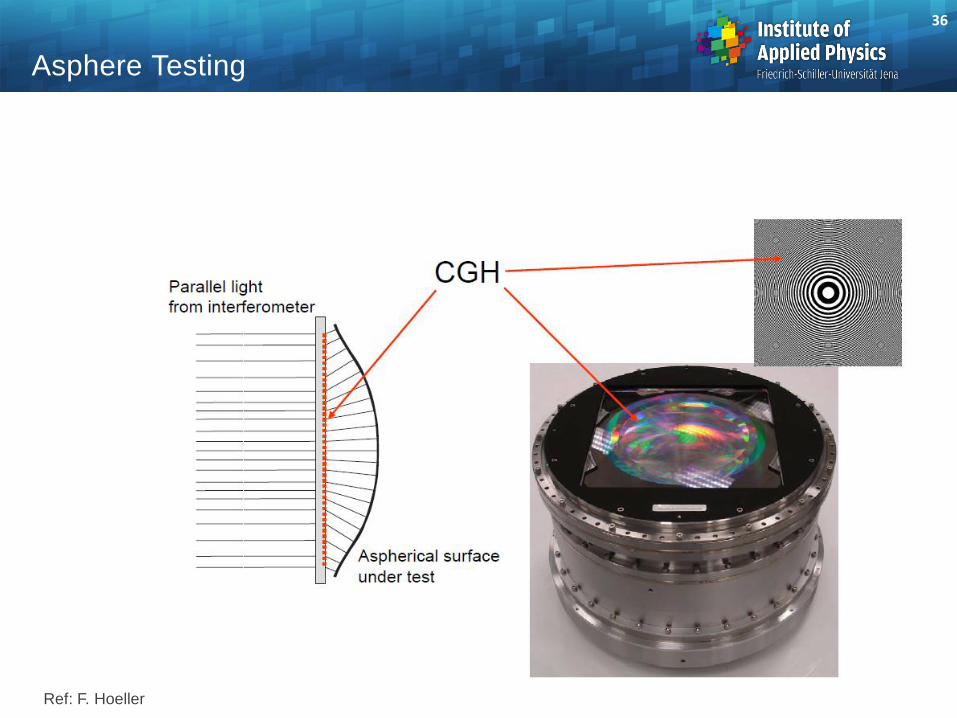
Asphere Testing

Creating a spherical wave for autocollimation

Ref: F. Hoeller

Compensating Null Systems

Ref: B. Dörband

Null compensation: improved accuracy by subtracting the main effect

Null optic: refractive or CGH

Different schemes for null compensation

31

K-system (null lens) generates aspherical replica of the wavefront for autokollimation

Samll residual perturbations of the autocollimation are resolved by the interferometer

Alignment of the K-lens is critical due to large spherical contributions

negative lens

increases beam

diameter

aspherical

surface

under testtest beam

positive lens generates

desired spherical

aberration wave

front

Test of Aspheres with Null Lenses

System configurations for

compensating null lenses

a) test surface convex

b) test surface convex

asphere steeper outside

c) test surface concave

asphere less steep outside

asphere

under test

here convex

null optical

lens

Test of Aspheres with Null Lenses

asphere under

test here steeper

outside

null lens

asphere

under test,

here outside

less steep

null lens

c) concave test surface

no intermediate focus

asphere steep outside

d) concave test surface

with intermediate focus

asphere less steep outside

e) concave test surface

with intermediate focus

and field lens for diameter

adaptation

concave asphere

less steep in outer

range

null lens with

intermediate focus

asphere concave

less steep outside

null lens with

intermediate focus

field lens

Test of Aspheres with Null Lenses

asphere

concave

null lens

Measuring of an asphere with (cheap) spherical reference mirror

Formation of the desired wavefront in front of the asphgere by computer generated

hologram

Measurement in transmission and reflection possible

Critical alignment of CGH

spherical mirror

autocollimation

asphere

under test

CGH

reshapes the

wavefront

light

source

spherical

phaseaspherical

phase

Test of Aspheres with CGH

36

Asphere Testing

Ref: F. Hoeller

37

CGH Null Test

1. CGH

2. Interferogram without CGH

(asphere)

3. Interferogram with CGH

Ref: R. Kowarschik

38

CGH Null Test

1. CGH in reflection 2. CGH in transmission

Ref: R. Kowarschik

39

CGH Metrology - Example

Fraunhofer IOF

9” CGH for secondary mirror of the

METi-satellite telescope

9” CGH for primary mirror of the

GAIA-satellite telescope

Critical Parameters:

• size up to 230mm x 230mm

• positioning accuracy

• data preparation !

• homogeneity of etching depth and

shape of grooves

wave-front accuracy

< 3nm (rms) demonstrated

Ref: U. Zeitner

In interferometer gradients are measured

Absolute error differences are of no meaning

Residual gradinet differences are essential for the performance of a null system

Example:

system 1 (red) is more benefitial, because the gradients are smaller

Test of Aspheres

System 2

h

W in

System 1

System 2

h

dW/dh

in / mm

System 1

General purpose:

- freeform surfaces are useful for compact systems with small size

- due to high performance requirements in imaging systems and limited technological

accuracy most of the applications are in illumination systems

- mirror systems are developed first in astronomical systems with complicated symmetry-free

geometry to avoid central obscuration

Definition:

- surfaces without symmetry

- reduced definition: plane symmetric or double plkane symmetric surfaces are freeforms

- special case: off-axis subaperture of circular symmetric aspheres

- segmented surfaces included ?

41

Freeform Systems: Motivation and Definition

Spectacle Freeform Lenses

Ref: W. Ulrich

42

Simultaneous correction of :

1. far, upper zone

2. near, lower zone

Continuous transition with reduced horizonthal field of view,

zone of progression

Approach in 1980: 800x800 patches, cubic spline despription, optimization with 107 parameters

Relaxed requirements on accuracy

near

zone

far zone

progression

zone no visionno vision

Free Shaped Eye-Glasses

43

44

Telescopes

Spectrometer

Lithographic projection systems

Reflective Freeform Systems

Lithographic Lens

Projection lenses in micro-Lithography

today uses freeform surfaces:

1. at 13.5 nm only mirrors are possible

2. at 193 nm the mirrors are helpful in

correcting the field flatness

45

46

PSD Ranges

Typical impact of spatial frequency

ranges on PSF

Low frequencies:

loss of resolution

classical Zernike range

High frequencies:

Loss of contrast

statistical

Large angle scattering

Mif spatial frequencies:

complicated, often structured

fals light distributions

log A2

Four

low spatial

frequency

figure errormid

frequency

range micro roughness

1/

oscillation of the

polishing machine,

turning ripple

10/D1/D 50/D

larger deviations in K-

correlation approach

ideal

PSF

loss of

resolution

loss of

contrast

large

angle

scattering

special

effects

often

regular

Diamond turning or milling creates regular ripple in nearly any case

- reason: point-like tooling and tool vs workpiece oscillations

- in case of final polishing effect is strongly reduced

Depending on the ratio of tool size and surface diameter this structure can not be described

by figure representations

47

Regular Ripple Errors

low

frequency

fit

residual

errors

original

a) b) c) d)

Metrology of Freeform Surfaces

Tactil / profilometer

Confocal microscopy

Optical coherence tomography

Hartmann sensor

Hartmann-Shack sensor

Deflectometry

Fringe projection

Interferometer with stitching

Interferometer with CGH for Null

compensation

Tilted Wave Interferometer

48

Measurement Approaches for Freeforms

volume

accuracy 10µm 0,1µm 0,001µm

1mm³

10mm³

100mm³

1000mm³

1µm 0,01µm

tactile

Fringe

projection

Interferometer

UA3P - 6

white light,

AFM,

Laser

scanner

Hartmann

Ref.: J. Heise

49

-50-

Measurement Approaches for Freeforms

Method Benefit Disadvantage

Tactile coordinate

measuring maschine

universal slow, damage,

expensive

Special maschines

ISARA , UA3P

universal

accurate

tactile, slow

expensive

Interferometer

with CGH

fast,

accurate

expensive, small

dynamic range

Fringe projection fast not accurate,

poor lateral resolution

Shack-Hartmann-Sensor fast small dynamic range

Ref.: J. Heise

Properties

50

Tactile Measurement

Ref: H. Hage / R.Börret

Scanning method

- Sapphire sphere probes shape

- slow

- only some traces are measured

Universal coordinate measuring machine

(CMM) as basic engine

Contact can damage the surface

Accuracy 0.2 m in best case

51

Tilted Wave Interferometer

Ref: H. Hage

Basic setup: Twyman-Green interferometer

Several points sources:

at least one is in autocollimation

to a sample point

Calibration complicated

Unusual interferogramms by superposition

52

Tilted Wave Interferometer

Ref: H. Hage

53

Interferometer with array of points sources (ITO / W. Osten, Mahr)

At least one source points

generates a subaperture

nearly perpendicular

Complicated data evaluation

Measurement by Subaperture Stitching

Ref: B. Dörband

Stitching of complete surface by subapertures:

dynamic range increased

Overlapping subapertures:

minimizing stitching errors due to

movement

Large computational effort

54

55

shape deviation after correction

and polishing: PV 2,5 µm

shape deviation after grinding: PV

26,2µm

Micro roughness 2,5x

(2,5x2,5mm2)

Micro roughness 40x

(0,15x0,15mm2) grinding

polishing

PSD measurement over manufacture flow

Ref: G. Günther

55

-56-

Positioning and Orientation of Freeforms

Fixation of a surface by spheres

Optical positioning of spheres by CGH

with stitching subapertures in catseye

setup

Higher accuracy in comparison to tactile

measurement

Ref.: M. Brunelle, Proc SPIE 9633 (2015)

polished

spheres

surface

56