Metrics for the Diurnal Cycle of Precipitation: Toward RoutineBenchmarks for Climate Models

CURT COVEY, PETER J. GLECKLER, CHARLES DOUTRIAUX, AND DEAN N. WILLIAMS

Program for Climate Model Diagnosis and Intercomparison, Lawrence Livermore National

Laboratory, Livermore, California

AIGUO DAI

University at Albany, State University of New York, Albany, New York

JOHN FASULLO AND KEVIN TRENBERTH

National Center for Atmospheric Research,a Boulder, Colorado

ALEXIS BERG

International Research Institute for Climate and Society, Columbia University, New York, New York

(Manuscript received 21 September 2015, in final form 11 January 2016)

ABSTRACT

Metrics are proposed—that is, a few summary statistics that condense large amounts of data from observations

or model simulations—encapsulating the diurnal cycle of precipitation. Vector area averaging of Fourier ampli-

tude and phase produces useful information in a reasonably small number of harmonic dial plots, a procedure

familiar from atmospheric tide research. The metrics cover most of the globe but down-weight high-latitude

wintertime ocean areas where baroclinic waves are most prominent. This enables intercomparison of a large

number of climate models with observations and with each other. The diurnal cycle of precipitation has features

not encountered in typical climate model intercomparisons, notably the absence of meaningful ‘‘average model’’

results that can be displayed in a single two-dimensional map. Displaying onemap permodel guides development

of the metrics proposed here by making it clear that land and ocean areas must be averaged separately, but

interpreting maps from all models becomes problematic as the size of a multimodel ensemble increases.

Global diurnal metrics provide quick comparisons with observations and among models, using the most

recent version of the CoupledModel Intercomparison Project (CMIP). This includes, for the first time inCMIP,

spatial resolutions comparable to global satellite observations. Consistent with earlier studies of resolution

versus parameterization of the diurnal cycle, the longstanding tendency of models to produce rainfall too early

in the day persists in the high-resolution simulations, as expected if the error is due to subgrid-scale physics.

1. Introduction

The purpose of this paper is to propose standard met-

rics for evaluating the diurnal timing of precipitation

in atmospheric general circulation models (GCMs). By

‘‘metrics’’ we mean a few numbers that condense large

amounts of output into summary statistics (Gleckler et al.

2008). Suchmetrics are useful in assessing overly frequent

occurrence of light rainfall (Trenberth et al. 2003; Dai 2006;

Stephens et al. 2010) and tropical precipitation occurring

too early in the day (Dai and Trenberth 2004; Dai 2006; Dai

et al. 2007; Kikuchi and Wang 2008). These problems im-

pair fundamental understanding of how climate emerges

Supplemental information related to this paper is available at the

Journals Online website: http://dx.doi.org/10.1175/JCLI-D-15-0664.s1.a The National Center for Atmospheric Research is sponsored

by the National Science Foundation.

Corresponding author address: Curt Covey, Program for Climate

Model Diagnosis and Intercomparison, Lawrence Livermore

National Laboratory, LLNL Mail Code L-103, 7000 East Ave.,

Livermore, CA 94550.

E-mail: covey1@llnl.gov

Denotes Open Access content.

15 JUNE 2016 COVEY ET AL . 4461

DOI: 10.1175/JCLI-D-15-0664.1

� 2016 American Meteorological Society

from the statistics of weather and also have important

practical consequences because the frequency and intensity

of precipitation impact human and natural systems.

Straightforward Fourier analysis provides both spatial

structures and time series at selected locations, sampling

data from a subset of models. Vector averaging over large

areas then provides the summarymetrics. As noted below,

more elaborate approaches exist but are less appropriate

for applying metrics to a large multimodel ensemble.

2. Data sources and algorithms

Simulations come from phase 5 of the Coupled Model

Intercomparison Project (CMIP5; Taylor et al. 2012),

including models with sufficient horizontal resolution to

be comparable to satellite observations of precipitation.

Table 1 shows that our two highest-resolution models

(GFDL HiRAM-C360 and MRI-AGCM3.2S) have grid

spacings as fine as or finer than 0.258 latitude/longitude,the resolution of commonly used observational datasets.

Each of these two models is paired with a lower-

resolution version (GFDL HiRAM-C180 and MRI-

AGCM3.2H). These four models only provide output

for the subset of CMIP in which sea surface temperatures

(SSTs) and sea ice concentrations are matched to obser-

vations for the period 1979–2008. In many ways, such

Atmospheric Model Intercomparison Project (AMIP)

boundary conditions give GCMs their best opportunity

for accurate climate simulation, though not necessarily

for coupled variations (Wang et al. 2005), as the SSTs do

not respond to surface forcing.Also, as the specified SSTs

do not contain diurnal variations, the diurnal cycle over

oceans is damped (Dai and Trenberth 2004; Covey et al.

2011), although this effect is not significant in our case,

as shown below.

Observations come from the 3-hourly, 0.258 latitude–

longitude resolution Tropical Rainfall Measuring Mission

(TRMM) 3B42 dataset coarchived with CMIP (Teixeira

et al. 2014). This is themost common source for global high-

time-frequency observations. It includes data from a wide

variety of sources in addition to the TRMM satellite and

covers over 75% of the globe (Huffman et al. 2007). Sim-

ulations and observations overlap during 1998–2008, but we

omit 1998 to minimize interannual variance (Fig. S1 in

supplemental material). All data used are publically avail-

able (http://cmip-pcmdi.llnl.gov/cmip5).

TABLE 1. CMIP5 3-hourly precipitation from AMIP forcing.a (Expansions of model name acronyms are available online at http://www.

ametsoc.org/PubsAcronymList.)

Model nameb Number of latitudes Number of longitudes Data volumec (GB)

1 BNU-ESMd 64 128 2.7

2 ACCESS1.0 145 192 9.2

3 ACCESS1.3p1 145 192 9.5

4 ACCESS1.3p2 145 192 9.5

5 BCC_CSM1.1(m)d 160 320 17

6 CCSM4 192 288 20

7 CMCC-CM 240 480 22

8 CNRM-CM5 128 256 11

9 EC-EARTH 160 320 18

10 FGOALS-g2 60 128 2.6

11 FGOALS-s2 60 128 2.7

12 GFDL HiRAM-C180 360 576 67

13 GFDL HiRAM-C360 720 1152 262

14 GISS-E2-Rp1 90 144 19

15 GISS-E2-Rp3 90 144 19

16 HadGEM2-Ad 145 192 9.1

17 INM-CM4.0 120 180 3.1

18 IPSL-CM5A-LR 96 96 2.8

19 IPSL-CM5A-MR 143 144 12

20 MIROC5 128 256 8.5

21 MRI-AGCM3.2H 320 640 67

22 MRI-AGCM3.2S 960 1920 603

23 MRI-CGCM3 160 320 18

24 NorESM1-M 96 144 4.6

Total: 1200

a AMIP: monthly mean sea surface temperature/sea ice concentration fields prescribed to match observations for 1979–2008.b Perturbed-physics version counts as a separate model (‘‘p’’ number in name).c For all 30 years of CMIP5–AMIP scenario and one ensemble member per model.d Not processed because of CMIP5 data structure issues, for example, nonstandard calendar. See http://cmip-pcmdi.llnl.gov/cmip5/errata/

cmip5errata.html.

4462 JOURNAL OF CL IMATE VOLUME 29

Python-based software (Williams et al. 2013) em-

ployed to study atmospheric tides in surface-pressure

fields (Covey et al. 2011) performs Fourier analysis in

time over the 10 Januaries and 10 Julys spanning 1999–

2008. This is equivalent to first averaging the time series

into a composite 24-h day and then applying Fourier

analysis (Covey and Gleckler 2014). We consider only

the first two harmonic components: diurnal (24 h) and

semidiurnal (12 h) periods. Although the daily cycle of

rainfall is incompletely described by two sinusoids, most

simulated and observed global data available—including

all data in this study—exist at 3-hourly time resolu-

tion. Thus, the semidiurnal harmonic, with only four

time points per cycle, already has large uncertainties,

while the terdiurnal harmonic (8 h) is close to the

limiting Nyquist period (6 h) and would add little real

information.

An alternative procedure identifies minimum and

maximum points in the composite diurnal cycle and

computes empirical orthogonal functions (EOFs; Kikuchi

and Wang 2008; Pritchard and Somerville 2009a,b;

Wang et al. 2011). Since EOFs are eigenvectors of ei-

ther the covariance or correlation matrix (which are

symmetric and positive definite), the EOF procedure is

mathematically guaranteed to produce an orthogonal

set of normal modes, each associated with a positive

eigenvalue that may be interpreted as the fractional

variance associated with the corresponding mode. But

from a physical point of view, some variations are more

suitable for EOF analysis than others. Real-valued

EOFs make each mode of variation a standing wave:

any location is either in phase or 1808 out of phase with

any other location. Thus, EOFs are a natural way to

study phenomena like the large-scale El Niño–La Niña‘‘seesaw’’ oscillation of warm surface water between the

western and eastern Pacific Oceans, but they are less

natural diagnostics for other processes. This limitation

may be overcome in various ways, including combined

analysis of different EOFs [see Wang et al. (2011, their

Fig. 2) for the diurnal cycle; Sperber and Kim (2012) for

the Madden–Julian oscillation] or complex EOFs cre-

ated from two-component vectors (e.g., Trenberth et al.

2000). Elaborated EOF analyses, however, seem less

appropriate than straightforward Fourier analysis for

first-look metrics.

3. Guidelines for metrics

Figure 1 presents the diurnal harmonic amplitude and

phase from the observations. Since warm seasons have

similar dynamics, Fig. 1 combines NorthernHemisphere

July and Southern Hemisphere January in both maps.

The resulting discontinuity at the equator is small.

(Corresponding cold season maps provide little ad-

ditional information because coherent diurnal varia-

tion outside the tropics is small; cf. Figs. S2–S5 in the

supplemental material.) The diurnal amplitude map

(Fig. 1, top) is normalized by the monthly mean (similar

to Dai et al. 2007), since otherwise an imprint of the

mean precipitation dominates. Grid points with ampli-

tudes greater than monthly mean values (ratios .1,

colored white) appear prominently in dry regions be-

cause of occasional showers occurring for one time step.

The Dirac delta function would give a ratio of exactly 2

for each Fourier component; in our results, very dry

regions give ratios close to 2 (Fig. S10 in the supple-

mental material). Wet regions generally give ratios #1,

although exceptions occur (e.g., in Florida) as explained

below in our discussion of individual gridpoint results.

The phasemap (bottom) explicitlymasks out areas where

the diurnal cycle is weak and hence phase is ill defined (gray

colors). Our criteria for a weak diurnal cycle are that either

monthlymean precipitation,0.75mmday21, about 25%of

the global average, or that the amplitude/monthly mean

ratio ,25%. This masking allows visualization of the main

features thatmetrics should encapsulate. It has theadditional

benefit of removing high-latitude wintertime ocean areas

where traveling synoptic storms (baroclinic waves) alias into

the diurnal signal. Some aliasing remains after masking, ap-

pearing asnorth–south stripes inphasemaps (e.g., inFig. S5).

This problemhas comeup inearlierwork (e.g., Fig. 5dofDai

et al. 2007). It appears more prominently in our graphics

because we display higher resolution. As shown in the next

section, however, our proposed summary metrics are not

significantly affected by these spurious phase stripes.

General conclusions from themaps are insensitive to the

choice of thresholds for data masking. Dai et al. (2007)

mask out areas where daily mean precipitation is less than

0.1mmday21 and find 1) diurnal amplitudes 30%–100%

of the mean over most land areas in summer and 10%–

30% over most ocean areas and 2) diurnal maxima in the

afternoon to evening hours over land andmidnight to early

morning over ocean. These conclusions also emerge from

inspection of both Fig. 1 and corresponding maps for the

semidiurnal harmonic (Figs. S6–S9 in the supplemental

material).

Mapping Fourier components at satellite resolution

visualizes observations that have been noted in regional

studies and in the EOF approach. Most prominent is a

summertime eastward propagation of rainfall in the

center of North America (Tripoli and Cotton 1989; Dai

et al. 1999; Jiang et al. 2006) that appears as north-to-

south stripes in the phase map. Also apparent are phase

discontinuities between land and ocean areas associated

with the sea breeze (Dai 2001; Pritchard and Somerville

2009b). Although regional phase propagation is not

15 JUNE 2016 COVEY ET AL . 4463

FIG. 1. TRMM3B42 composites of July in the NorthernHemisphere and January in the SouthernHemisphere, for (top) ratio of diurnal

harmonic amplitude to monthly mean precipitation and (bottom) diurnal harmonic phase expressed as LST of maximum precipitation. In

the top map, ratios greater than unity are colored white (where 24-h Fourier amplitude for the diurnal cycle exceeds the mean monthly

value). The few grid points where no precipitation occurs during the study period are colored gray. In the bottommap, areas where either

monthly mean precipitation or its diurnal cycle is weak are colored gray (using masking criteria described in the text). Black dots in both

maps locate grid points selected for later time series analysis.

4464 JOURNAL OF CL IMATE VOLUME 29

represented in the large-scale average metrics we pro-

pose below, the very sharp distinction between land and

ocean areas in Fig. 1 makes it clear that averagesmust be

taken separately over each.

For CMIP’s highest-resolution GCMs, diurnal am-

plitudes are in fair agreement with observations (Figs. 2

and S2), but corresponding phases give warm season

rainfall too early in the day, at least over land (Figs. 3

and S3). The semidiurnal harmonic exhibits similar

errors (Figs. S6 and S7). Prior work revealed this prob-

lem in earlier, lower-resolution models (see above) as

well as in higher resolutions, up to the point where ex-

plicitly simulated convection can replace subgrid-scale

parameterizations (Sato et al. 2009; Dirmeyer et al.

2012). An important caveat is that TRMM 3B42 phase

values are biased late by up to 3h because the 3B42 al-

gorithm includes outgoing longwave radiation (OLR)

and thus includes high cold clouds, which peak after

surface precipitation (Dai et al. 2007; Kikuchi andWang

2008). This bias is larger than CMIP time-sampling

errors (Berg et al. 2014; Zhou et al. 2015). Nevertheless,

the problem with too-early climate model rainfall also

appears in surface in situ observations, for example, in the

North American Great Plains, as discussed below in

conjunction with Fig. 4. We show in conjunction with

Fig. 5 that average CMIP bias exceeds the TRMM ob-

servational uncertainty.

A noteworthy feature of Figs. 2 and 3 is a close re-

semblance of MRI-AGCM3.2S and MRI-AGCM3.2H,

suggesting that subgrid-scale ‘‘column physics’’ rather

than explicitly resolved dynamics is responsible for model

errors. GFDL HiRAM-C360 and GFDL HiRAM-C180

also resemble each other, except for diurnal harmonic

phase in Australia and some coastal zones, where the

C360 version is nearly 1808 out of phase with the C180

version. Since column physics is identical except for tun-

ing parameters in the GFDL HiRAM versions archived

in CMIP5 (S.-J. Lin 2015, personal communication), their

differences probably involve explicitly resolved dynamics.

Itmaybe relevant thatGFDLHiRAMuses a cubed-sphere

grid that inevitably generates discontinuities (Putman and

Lin 2007).

Figures 1–3 come from Fourier analysis at each indi-

vidual grid point. To sample this process, we choose 7 of

the 10 points in Fig. 4 of Dai et al. (2007) plus the

Southern Great Plains site of the Atmospheric Radiation

Measurement program (ARM SGP). These eight points

are marked by black dots in Figs. 1–3; results for each are

shown in Fig. 4. Observed composite diurnal variations

are fitted rather well by only the first two harmonic

FIG. 2. Amplitude ratios, as in the topmap in Fig. 1, forAMIP simulations by the four highest-resolutionCMIP5models: (top left) 0.58 and (topright) 0.258 GFDL model and (bottom left) high- and (bottom right) super-high-resolution MRI model.

15 JUNE 2016 COVEY ET AL . 4465

components (black dots and lines) wherever a coherent

diurnal cycle exists. Observed rainfall at the Florida and

Yangtze River valley locations peaks in late afternoon

and evening hours, typical ofwarm land areas (Figs. 4a,b).

Northeast Argentina and the ARM SGP site, both in

areas of zonal propagation (Fig. 1), have broad maxima

(Figs. 4c,d). The Pacific warm pool and Indian Ocean

points experience mainly 24-h cycles of low amplitude

with peaks occurring in early morning, typical of the

tropical oceans (Figs. 4e,f). The final two grid points in

Fig. 4 exemplify higher-latitude ocean areas with no ob-

vious diurnal cycle (Figs. 4g,h).

The Florida grid point (Fig. 4a) has a particularly simple

diurnal cycle with very little rainfall in the morning and

one distinct peak in late afternoon–early evening. There-

fore, Fourier analysis gives a ratio of harmonic amplitude

to mean value of 1.3, lying in between 1 (for a pure sine

wave) and 2 (for a delta function). The same results are

obtained for other wet locations when rainfall occurs at

restricted times of day (Fig. S10).

We have added 61s error bars to the observed

3-hourly values plotted in Fig. 4, with s defined as stan-

dard error of the composite mean, that is, we divided the

standard deviation of the data points contributing to

each local standard time (LST) byffiffiffiffiffiffiffiffi

310p

. This un-

derestimates the true uncertainty by assuming that each

of the 310 days of a given month during 1999–2008 is

independent. In spite of this underestimate, the error

bars are rather large, not only at locations where one

must question the significance of Fourier analysis

(Figs. 4g,h) but also in locations with coherent diurnal

cycles. Applying a rigorous statistical test could there-

fore suppress physically important results, for example,

the well-established morning rainfall peaks observed in

the tropical Pacific and Indian Oceans (Figs. 4e and 4f;

compare Figs. 4f and 4g in Dai et al. 2007) and the peak

around midnight at the ARM SGP site (Fig. 4c).

Therefore, we retain the less severe constraints of the

masking procedure defined above.

The ARM data are particularly important because they

are ground based and in excellent agreement with TRMM

3B42 (cf. Fig. 1b in Jiang et al. 2006). At this location,

occasional storms produce high rainfall rates while most

time bins record zero rain. In statistical terms, large

skewness moves the standard deviation far out beyond

the mean value because the distribution is more Poisson-

like thanGaussian (Fig. S11 in the supplementalmaterial).

Uncertainty in average amplitude and phase, however, is

smaller than the uncertainty at each LST and location.

Also, the central limit theorem implies that statistics

become more Gaussian as more space–time points are

averaged together. Accordingly, the summary metrics

presented in Fig. 5 below are fairly robust.

In contrast to observations, modeled rainfall (colored

dots) in Fig. 4 is quite noisy. Often its pattern is poorly fit

by low-order Fourier harmonics (or other simple curves),

FIG. 3. As in Fig. 2, but for phase, with definitions and thresholds for masking (gray colors) matching the bottom map in Fig. 1.

4466 JOURNAL OF CL IMATE VOLUME 29

FIG. 4. Composite diurnal time series from TRMM 3B42 observations (black dots) and from the four highest-resolution

CMIP5 models (colored dots), at the eight sample points shown in the maps above. Models are color coded as described

in the figure legend. Observed time points are fit by (dashed lines) the diurnal harmonic only and by (solid lines) the

combination of diurnal and semidiurnal harmonics, with error bars showing standard error of the mean.

15 JUNE 2016 COVEY ET AL . 4467

implying that Fourier amplitudes and phases at single

grid points are not ideal for its decomposition. Florida

and the Yangtze River valley sample the widespread

land areas where observed precipitation peaks in late

afternoon–early evening, and the models rain too early in

the day, as noted above. At other points, however, a sys-

tematic difference between model simulations and obser-

vations is not evident. The implication is that model output

needs to be averaged over more than one grid point, either

‘‘by eye’’ in visual inspection of maps, or more systemati-

cally as proposed below.

4. Proposed metrics

Careful inspection of several maps per model is im-

practical in a largemultimodel ensemble. Zonal averaging

provides some insight if land and ocean areas are each

homogeneous and averaged separately (see top panels in

Fig. 17 of Dai 2006). Here we propose an extension of this

procedure to area averages. The ‘‘harmonic dial’’ diagram

originally developed in atmospheric tide research—

treating the amplitude and phase of each harmonic com-

ponent as a two-dimensional vector—provides the most

appropriate display graphic (see section 1.2B in Chapman

and Lindzen 1970). Averaging separately over all land

and all ocean is a reasonable first step because the ob-

served phase is roughly uniform (apart from areas of

phase propagation).

In this approach, adding vectors during the averaging

process automatically down-weights areas where the

diurnal cycle is weak. There is no need to choose arbi-

trary thresholds for data masking. In any case the choice

of thresholds or filtering makes little difference. Table 2

compares averages computed using no filtering or

masking of any kind with analogous averages using the

same filtering procedure as in Figs. 1 and 3. Averaged

phases with and without filtering are virtually identical.

Averaging over the spurious phase stripes that arise

from synoptic time-scale aliasing (e.g., appearing in the

bottom panel of Fig. 1) leads to cancellation of vector

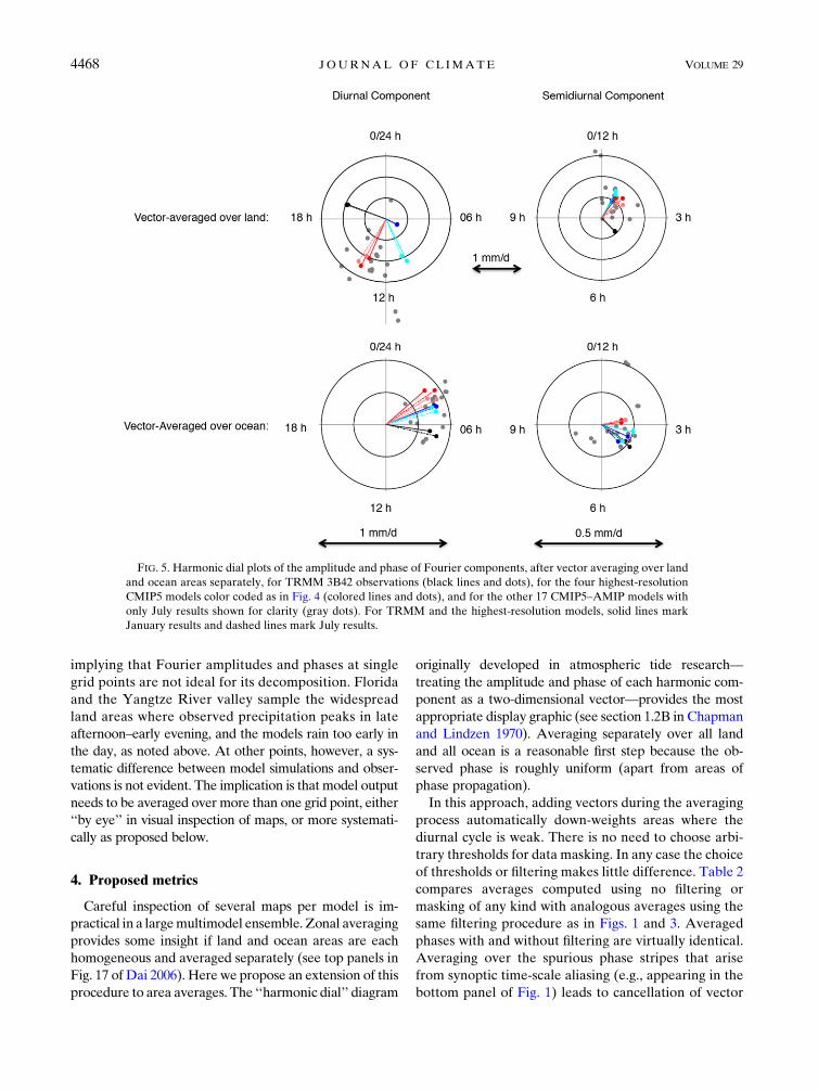
FIG. 5. Harmonic dial plots of the amplitude and phase of Fourier components, after vector averaging over land

and ocean areas separately, for TRMM 3B42 observations (black lines and dots), for the four highest-resolution

CMIP5 models color coded as in Fig. 4 (colored lines and dots), and for the other 17 CMIP5–AMIP models with

only July results shown for clarity (gray dots). For TRMM and the highest-resolution models, solid lines mark

January results and dashed lines mark July results.

4468 JOURNAL OF CL IMATE VOLUME 29

sums because the phases run through one or more 360

cycles; hence, this aliasing does not affect the end results.

Averaged amplitudes are increased by the filtering, be-

cause it masks out shorter vectors, but the inflation factor

is roughly uniform and thus intercomparison of ampli-

tudes from different data sources is not meaningfully af-

fected. In short, our proposed metrics are not sensitive to

masking strategy. Therefore, the simplest andbest strategy

is to use no masking at all when computing area averages.

Figure 5 shows resulting plots for TRMM 3B42 ob-

servations and for all models in Table 1. No masking or

filtering is used in producing this figure. Each pair of

maps (like Fig. 1) has become a pair of points (one for

January and one for July) on each of four harmonic dials

representing diurnal versus semidiurnal components

and land versus ocean averaging. Land areas (Fig. 5, top

panels) exhibit considerable scatter among the models,

but both the diurnal and semidiurnal components from

most models have vector-averaged lengths comparable

to observations. A notable exception is GFDLHiRAM-

C360 (blue lines and points). In this model, the out-of-

phase spatial variation noted above produces a weak

mean amplitude. This problem arises occasionally in the

harmonic dial approach, for example, in Fig. 5 of the tide

study of de Argandoña et al. (2010).

The vast majority of models, however, produce co-

herent spatial averages over land that reveal systematic

phase errors consistent with Figs. 1–3. The difference

between TRMM and the models, 6–10 h in the domi-

nant diurnal component, is much greater than either

the 2–3-h observational error estimated by Dai et al.

(2007) or the 3-h observational error estimated by

Kikuchi and Wang (2008). For the weaker semidiurnal

component, the difference between TRMM and the

models is roughly 3 h on average, perhaps within ob-

servational uncertainty. Still, model rainfall peaks

systematically earlier than the observations. In both

observations and models the semidiurnal component

sharpens the diurnal peak, for example, TRMM has a

diurnal maximum around 1900 LST reinforced by

semidiurnal maxima around 1600 LST.

For ocean areas the length scale in Fig. 5 (bottom

panels) is expanded to accommodate considerably smaller

amplitudes. For the diurnal component, nearly all models

have amplitudes roughly comparable to observations

but peak times systematically earlier. These oceanic

diurnal results from the AMIP-type runs are consistent

with those from the coupled model simulations (Dai

2006; Flato et al. 2013). It seems that the removal of the

SST diurnal cycle has little effect on the mean diurnal

cycle of oceanic precipitation. The semidiurnal compo-

nent over oceans is small in both models and observa-

tions, consistent with Fig. 4.TABLE2.V

ector-averagedspatialm

eanswithoutandwithmasking:amplitude(m

mday2

1),phase

(LST)(m

askedresultsin

curlybrackets).Obs4MIPsstandsforObservationsforModel

IntercomparisonProjects.

Obs4MIPs/TRMM3B42

GFDLHiR

AM-C

180

GFDLHiR

AM-C

360

MRI-AGCM3.2H

MRI-AGCM3.2S

July

diurnal

Lan

d0.976,19.355{1.634,19.398}

0.955,9.015

{1.869,

9.097}

0.284,6.331

{0.514,

6.626}

1.191,12.663{2.453,

12.716}

1.255,12.344{2.307,

12.368}

Ocean

0.577,7.011

{0.401,6.867}

0.400,3.520

{0.510,

3.956}

0.416,3.185

{0.545,

3.449}

0.439,2.742

{0.628,

3.018}

0.462,2.152{0.651,

2.358}

July

semidiurnal

Lan

d0.439,4.518

{0.773,4.586}

0.634,11.519{1.964,

11.421}

0.470,11.515{1.175,11.486}

0.587,0.421

{1.946,

0.448}

0.681,0.038{1.712,

0.039}

Ocean

0.112,4.160

{0.145,4.192}

0.104,2.772

{0.047,

2.532}

0.092,3.021

{0.080,

3.028}

0.095,1.136

{0.056,

2.133}

0.079,1.073{0.070,

2.014}

January

diurnal

Lan

d0.948,19.411{1.605,19.398}

1.109,8.773

{2.136,

8.838}

0.289,6.216

{0.542,

6.490}

0.989,12.340{1.979,

12.379}

1.010,12.031{1.931,

12.018}

Ocean

0.344,6.559

{0.485,6.748}

0.381,3.134

{0.471,

3.515}

0.402,3.024

{0.489,

3.275}

0.380,2.364

{0.521,

2.790}

0.399,1.738{0.558,

2.023}

January

semidiurnal

Lan

d0.457,4.565

{0.803,4.602}

0.729,11.402{2.126,

11.338}

0.611,11.473{1.501,11.471}

0.507,0.020

{1.571,

0.049}

0.564,11.650{1.393,

11.636}

Ocean

0.139,4.283

{0.175,4.323}

0.124,1.914

{0.079,

1.973}

0.112,2.321

{0.103,

2.368}

0.094,1.129

{0.075,

2.162}

0.077,1.303{0.082,

2.085}

15 JUNE 2016 COVEY ET AL . 4469

5. Future extensions

The metrics proposed here would be only a first step

in quantifying the diurnal cycle. Vector means could

also be computed for smaller scales than the all-land

and all-ocean areas shown in Fig. 5, giving more

information about spatial variations. TheGFDLHiRAM-

C360 problem arising from unwanted phase cancella-

tion (Fig. 5a) could be ‘‘solved’’ by ad hoc division of

land into coastal areas versus interior areas, but this

seems arbitrary. A physically based geographical di-

vision suggested by Kikuchi and Wang (2008, their

Fig. 10) might be more informative, but it would not

solve the GFDL HiRAM-C360 problem, nor would the

geographical regions necessarily remain fixed when the

climate changes.

In addition to area-mean bias, vector averaging can

be extended to other familiar statistics by simply

replacing the multiplication of numbers with the scalar

(dot) product of vectors. For example, the spatial var-

iance of a vector field x becomes s2x 5 hx0 � x0i, where

the angle brackets denote area means and the primes

denote differences from area means, for example,

x0 5 x2 hxi. The resulting algebra expresses the cen-

tered mean-square difference (i.e., the difference after

removing the area-mean bias of each field) exactly as

for scalar fields in a Taylor (2001) diagram. The mean-

square difference between two vector fields x and

y becomes h(x2 y) � (x2 y)i5 (hxi2 hyi) � (hxi2 hyi)1s2x 1s2

y 2 2Rxysxsy, where Rxy is their correlation

hx0 � y0i/sxsy. In this equation, the scalar product on

the right-hand side is the squared difference of vec-

tor means, given by constructing arrows that join

observed with model points in Fig. 5. The remaining

terms on the right form the centered mean-square

difference.

Taylor diagrams reasonably summarize model be-

havior if the bias is small compared with the centered

root-mean-square (RMS) error. This is true for monthly

mean precipitation but not true for its diurnal cycle. The

substantial phase discrepancies between models and

observations discussed above are coherent across wide

areas. Thus, Taylor diagrams constructed from vector

statistics would probably not be meaningful for the

diurnal cycle of precipitation, although one could com-

pute results analogous to Fig. 5 for any region. For ex-

ample, dividing North America into a few domains with

different character would raise the question of how

much the phase can be allowed to vary within a domain

before it becomes significantly different. Here some

form of classification or EOF analysis might apply, but a

key point is that one can reduce the dimensionality

many fold.

Finally, we note that precipitation is only one of 23

fields archived at 3-hourly frequency in CMIP5. This

database remains a largely unexplored source of in-

formation about the diurnal cycle of near-surface fields.

Relationships between different fields may aid satellite re-

trieval algorithms, as well as climate model development.

Acknowledgments. We thank Karl Taylor for math-

ematical consultation, the Working Group on Coupled

Modelling for CMIP planning, and themodelers (Table

1) for providing output. We also thank our colleagues

Shaocheng Xie and Chengzhu Zhang for useful dis-

cussion of the relationship between ARM and TRMM

observations. Work was performed under auspices of

the DOE Office of Science by Lawrence Livermore

National Laboratory under Contract DE-AC52-

07NA27344, at the National Center for Atmospheric

Research, and at Columbia University and the State

University of New York. We acknowledge funding

from NSF Grants AGS-1353740 and AGS-1331375,

DOE Awards DE-SC0012602 and DE-SC0012711,

and NOAA Award NA15OAR4310086.

REFERENCES

Berg, A., K. Findell, and A. Gianini, 2014: Assessing the

evaporation-precipitation feedback in CMIP5 models. 2014

Fall Meeting, San Francisco, CA, Amer. Geophys. Union,

Abstract 31314.

Chapman, S., and R. S. Lindzen, 1970: Atmospheric Tides.

D. Reidel, 200 pp.

Covey, C., and P. Gleckler, 2014: Standard diagnostics for the di-

urnal cycle of precipitation. Lawrence Livermore National

Laboratory Tech. Rep. LLNL-TR-659685, 11 pp. [Available

online at https://e-reports-ext.llnl.gov/pdf/780868.pdf.]

——, A. Dai, D. Marsh, and R. S. Lindzen, 2011: The surface-

pressure signature of atmospheric tides in modern climate

models. J. Atmos. Sci., 68, 495–514, doi:10.1175/2010JAS3560.1.

Dai, A., 2001: Global precipitation and thunderstorm frequencies.

Part II: Diurnal variations. J. Climate, 14, 1112–1128,

doi:10.1175/1520-0442(2001)014,1112:GPATFP.2.0.CO;2.

——, 2006: Precipitation characteristics in eighteen coupled

climate models. J. Climate, 19, 4605–4630, doi:10.1175/

JCLI3884.1.

——, andK. E. Trenberth, 2004: The diurnal cycle and its depiction in

the Community Climate System Model. J. Climate, 17, 930–951,

doi:10.1175/1520-0442(2004)017,0930:TDCAID.2.0.CO;2.

——, F. Giorgi, and K. E. Trenberth, 1999: Observed and model

simulated precipitation diurnal cycle over the contiguous

United States. J. Geophys. Res., 104, 6377–6402, doi:10.1029/

98JD02720.

——, X. Lin, and K.-L. Hsu, 2007: The frequency, intensity, and

diurnal cycle of precipitation in surface and satellite obser-

vations over low- and mid-latitudes. Climate Dyn., 29, 727–

744, doi:10.1007/s00382-007-0260-y.

de Argandoña, J. D., A. Ezcurra, J. Sáenz, B. Campistron,

G. Ibarra-Berastegi, and F. Saïd, 2010: Atmospheric tides

over the Pyrenees: Observational study and numerical

4470 JOURNAL OF CL IMATE VOLUME 29

simulation. Quart. J. Roy. Meteor. Soc., 136, 1263–1274,

doi:10.1002/qj.626.

Dirmeyer, P. A., and Coauthors, 2012: Simulating the diurnal cycle

of rainfall in global climate models: Resolution versus pa-

rameterization. Climate Dyn., 39, 399–418, doi:10.1007/

s00382-011-1127-9.

Flato, G., and Coauthors, 2013: Evaluation of climate models.

Climate Change 2013: The Physical Science Basis, T. F. Stocker

et al., Eds., Cambridge University Press, 741–866.

Gleckler, P. J., K. E. Taylor, and C. Doutriaux, 2008: Performance

metrics for climate models. J. Geophys. Res., 113, D06104,

doi:10.1029/2007JD008972.

Huffman, G. R., and Coauthors, 2007: The TRMM Multi-

satellite Precipitation Analysis (TMPA): Quasi-global,

multiyear, combined-sensor precipitation estimates at

fine scales. J. Hydrometeor., 8, 38–55, doi:10.1175/

JHM560.1.

Jiang, X., N.-G. Lau, and S. A. Klein, 2006: Role of eastward

propagating convection systems in the diurnal cycle and sea-

sonal mode of rainfall over the U.S. Great Plains. Geophys.

Res. Lett., 33, L19809, doi:10.1029/2006GL027022.

Kikuchi, K., and B. Wang, 2008: Diurnal precipitation regimes in

the global tropics. J. Climate, 21, 2680–2696, doi:10.1175/

2007JCLI2051.1.

Pritchard,M. S., andR. C. Somerville, 2009a: Empirical orthogonal

function analysis of the diurnal cycle of precipitation in a

multi-scale climate model. Geophys. Res. Lett., 36, L05812,

doi:10.1029/2008GL036964.

——, and ——, 2009b: Assessing the diurnal cycle of precipitation

in a multi-scale climate model. J. Adv. Model. Earth Syst., 1,

doi:10.3894/JAMES.2009.1.12.

Putman, W. M., and S.-J. Lin, 2007: Finite-volume transport on

various cubed-sphere grids. J. Comput. Phys., 227, 55–78,

doi:10.1016/j.jcp.2007.07.022.

Sato, T., H. Miura, M. Satoh, Y. N. Takayabu, and Y. Wang, 2009:

Diurnal cycle of precipitation in the tropics simulated in a

global cloud-resolving model. J. Climate, 22, 4809–4826,

doi:10.1175/2009JCLI2890.1.

Sperber, K. R., and D. Kim, 2012: Simplified metrics for the

identification of the Madden-Julian oscillation in models. At-

mos. Sci. Lett., 13, 187–193, doi:10.1002/asl.378.

Stephens, G. L., and Coauthors, 2010: Dreary state of precipitation

in global models. J. Geophys. Res., 115, D24211, doi:10.1029/

2010JD014532.

Taylor, K. E., 2001: Summarizing multiple aspects of model per-

formance in a single diagram. J. Geophys. Res., 106, 7183–7192, doi:10.1029/2000JD900719.

——,R. J. Stouffer, andG.A.Meehl, 2012: An overview of CMIP5

and the experiment design. Bull. Amer. Meteor. Soc., 93, 485–

498, doi:10.1175/BAMS-D-11-00094.1.

Teixeira, J., D. Waliser, R. Ferraro, P. Gleckler, T. Lee, and

G. Potter, 2014: Satellite observations for CMIP5: The genesis

of Obs4MIPs. Bull. Amer. Meteor. Soc., 95, 1329–1334,

doi:10.1175/BAMS-D-12-00204.1.

Trenberth, K. E., D. P. Stepaniak, and J. M. Caron, 2000: The

global monsoon as seen through the divergent atmospheric

circulation. J. Climate, 13, 3969–3993, doi:10.1175/1520-0442(2000)013,3969:TGMAST.2.0.CO;2.

——, A. Dai, R. M. Rasmussen, and D. B. Parsons, 2003: The

changing character of precipitation. Bull. Amer. Meteor. Soc.,

84, 1205–1217, doi:10.1175/BAMS-84-9-1205.

Tripoli, G. J., and W. R. Cotton, 1989: Numerical study of an ob-

served orogenic mesoscale convective system. Part 1: Simu-

lated genesis and comparison with observations. Mon. Wea.

Rev., 117, 273–304, doi:10.1175/1520-0493(1989)117,0273:

NSOAOO.2.0.CO;2.

Wang, B., Q. Ding, X. Fu, I.-S. Kang, K. Jin, J. Shukla, and

F. Doblas-Reyes, 2005: Fundamental challenge in simulation

and prediction of summer monsoon rainfall. Geophys. Res.

Lett., 32, L15711, doi:10.1029/2005GL022734.

——,H.-J. Kim,K.Kikuchi, andA.Kitoh, 2011:Diagnosticmetrics

for evaluation of annual and diurnal cycles. Climate Dyn., 37,941–955, doi:10.1007/s00382-010-0877-0.

Williams, D. N., and Coauthors, 2013: Ultrascale visualization of

climate data. Computer, 46, 68–76, doi:10.1109/MC.2013.119.

Zhou, L.,M. Zhang,Q. Bao, andY. Liu, 2015:On the incident solar

radiation in CMIP5 models. Geophys. Res. Lett., 42, 1930–

1935, doi:10.1002/2015GL063239.

15 JUNE 2016 COVEY ET AL . 4471