Metrics for Offline Evaluation of Prognostic … for Offline Evaluation of Prognostic Performance...

International Journal of Prognostics and Health Management

1

Metrics for Offline Evaluation of Prognostic Performance

Abhinav Saxena1, Jose Celaya1, Bhaskar Saha2, Sankalita Saha2, and Kai Goebel3

1SGT Inc., NASA Ames Research Center, Intelligent Systems Division, Moffett Field, CA 94035, USA [email protected] [email protected]

2MCT Inc., NASA Ames Research Center, Intelligent Systems Division, MS 2694, Moffett Field, CA 94035, USA

[email protected] sankalita.saha[email protected]

3NASA Ames Research Center, Intelligent Systems Division, MS 2694, Moffett Field, CA 94035, USA

[email protected]

ABSTRACT

Prognostic performance evaluation has gained significant attention in the past few years.*Currently, prognostics concepts lack standard definitions and suffer from ambiguous and inconsistent interpretations. This lack of standards is in part due to the varied enduser requirements for different applications, time scales, available information, domain dynamics, etc. to name a few. The research community has used a variety of metrics largely based on convenience and their respective requirements. Very little attention has been focused on establishing a standardized approach to compare different efforts. This paper presents several new evaluation metrics tailored for prognostics that were recently introduced and were shown to effectively evaluate various algorithms as compared to other conventional metrics. Specifically, this paper presents a detailed discussion on how these metrics should be interpreted and used. These metrics have the capability of incorporating probabilistic uncertainty estimates from prognostic algorithms. In addition to quantitative assessment they also offer a comprehensive visual perspective that can be used in designing the prognostic system. Several methods are suggested to customize these metrics for different applications. Guidelines are provided to help choose one method over another based on distribution characteristics. Various issues faced by prognostics and its performance evaluation are discussed followed by a formal notational framework to help standardize subsequent developments.

* This is an openaccess article distributed under the terms of the Creative Commons Attribution 3.0 United States License, which permits unrestricted use, distribution, and reproduction in any medium, provided the original author and source are credited.

1. INTRODUCTION

In the systems health management context, prognostics can be defined as predicting the Remaining Useful Life (RUL) of a system from the inception of a fault based on a continuous health assessment made from direct or indirect observations from the ailing system. By definition prognostics aims to avoid catastrophic eventualities in critical systems through advance warnings. However, it is challenged by inherent uncertainties involved with future operating loads and environment in addition to common sources of errors like model inaccuracies, data noise, and observer faults among others. This imposes a strict validation requirement on prognostics methods to be proven and established though a rigorous performance evaluation before they can be certified for critical applications. Prognostics can be considered an emerging research field. Prognostic Health Management (PHM) has in most respects been accepted by the engineered systems community in general, and by the aerospace industry in particular, as a promising avenue for managing the safety and cost of complex systems. However, for this engineering field to mature, it must make a convincing business case to the operational decision makers. So far, in the early stages, focus has been on developing prognostic methods themselves and very little has been done to define methods to allow comparison of different algorithms. In two surveys on methods for prognostics, one on datadriven methods (Schwabacher, 2005) and one on artificialintelligencebased methods (Schwabacher & Goebel, 2007), it can be seen that there is a lack of standardized methodology for performance evaluation and in many cases performance evaluation is not even formally addressed. Even the current ISO standard by International Organization for Standards (ISO, 2004) for prognostics in condition monitoring and diagnostics of machines lacks a firm

https://ntrs.nasa.gov/search.jsp?R=20100039169 2018-06-06T08:40:28+00:00Z


2

definition of any such methods. A dedicated effort to develop methods and metrics to evaluate prognostic algorithms is needed. Metrics can create a standardized language with which technology developers and users can communicate their findings and compare results. This aids in the dissemination of scientific information as well as decision making. Metrics could also be viewed as a feedback tool to close the loop on research and development by using them as objective functions to be optimized as appropriate by the research effort. Recently there has been a significant push towards crafting suitable metrics to evaluate prognostic performance. Researchers from government, academia, and industry are working closely to arrive at useful performance measures. With these objectives in mind a set of metrics have been developed and proposed to the PHM community in the past couple years (Saxena, Celaya, Saha, Saha, & Goebel, 2009b). These metrics primarily address algorithmic performance evaluation for prognostics applications but also have provisions to link performance to higher level objectives through performance parameters. Based on experience gained from a variety of prognostic applications these metrics were further refined. The current set of prognostics metrics aim to tackle offline performance evaluation methods for applications where runtofailure data are available and true EndofLife (EoL) is known a priori. They are particularly useful for the algorithm development phase where feedback from the metrics can be used to finetune prognostic algorithms. These metrics are continuously evolving and efforts are underway towards designing online performance metrics. This will help associate a sufficient degree of confidence to the algorithms and allow their application in real insitu environments.

1.1 Main Goals of the Paper This paper presents a discussion on prognostics metrics that were developed in NASA’s Integrated Vehicle Health Management (IVHM) project under the Aviation Safety program (NASA, 2009). The paper aims to make contribution towards providing the reader with a better understanding of: the need for separate class of prognostic performance metrics

difference in user objectives and corresponding needs from a performance evaluation view point

what can or cannot be borrowed from other forecasting related disciplines

issues and challenges in prognostics and prognostic performance evaluation

key prognostic concepts and a formal definition of a prognostic framework

new performance evaluation metrics, their application and interpretation of results

research issues and other practical aspects that need to be addressed for successful deployment of prognostics

1.2 Paper Organization Section 2 motivates the development of prognostic metrics. A comprehensive literature review of performance assessment for prediction/forecasting applications is presented in section 3. This section also categorizes prognostic applications in several classes and identifies the differences from other forecasting disciplines. Key aspects for prognostic performance evaluation are discussed in Section 4. Technical development of new performance metrics and a mathematical framework for the prognostics problem are then presented in detail in Section 5. Section 6 follows with a brief case study as an example for application of these metrics. The paper ends with future work proposals and concluding discussions in Sections 7 and 8 respectively.

2. MOTIVATION

This research is motivated by twofold benefits of establishing standard methods for performance assessment (see Figure 1). One, it will help create a foundation for assessing and comparing performance of various prognostics methods and approaches as far as low level algorithm development is concerned. Two, from a topdown perspective, it will help generate specifications for requirements that are imposed by costbenefit and risk constraints at different system lifecycle stages in order to ensure safety, availability, and reliability. In this paper we discuss these metrics primarily in the context of the first benefit and only a brief discussion is provided on requirements specification.

2.1 Prognostic Performance Evaluation Most of the published work in the field of prognostics has been exploratory in nature, such as proofofconcepts or oneoff applications. A lack of standardized guidelines has led researchers to use common accuracy and precision based metrics, mostly borrowed from the diagnostics domain. In some cases these are modified on an ad hoc basis to suit specific applications. This makes it rather difficult to compare various efforts and choose a winning candidate from several algorithms, especially for safety critical applications. Research efforts are focusing on developing algorithms that can provide a RUL estimate, generate a confidence bound around the predictions, and be easily integrated with existing diagnostic systems. A key step in successful


3

deployment of a PHM system is prognosis certification. Since prognostics is still considered relatively immature (as compared to diagnostics), more focus so far has been on developing prognostic methods rather than evaluating and comparing their performances. Consequently, there is a need for dedicated attention towards developing standard methods to evaluate prognostic performance from a viewpoint of how post prognostic reasoning will be integrated into the health management decision making process.

RequirementVariables

PerformanceSpecifications

PerformanceEvaluation

Algorithm Fine-tuning

Fault evolution

rate

Cost of unscheduled

repairs

Cost of lost or incomplete

missionCost of incurred damages

Failure criticality

Time required for repair actions

Best achievable algorithm

fidelity

Algorithm Selection

Desired minimum

performance criteria

Algorithm Complexity

Time needed to make a

prediction

Prognostics Metrics Prognostics Metrics

Prognostics Metrics

Logistics efficiency

Figure 1: Prognostics metrics facilitate performance evaluation and also help in requirements specification.

2.2 Prognostic Requirements Specification Technology Readiness Level (TRL) for the current prognostics technology is considered low. This can be attributed to several factors lacking today such as assessment of prognosability of a system, concrete Uncertainty Representation and Management (URM) approaches,

stringent Validation and Verification (V&V) methods for prognostics

understanding of how to incorporate risk and reliability concepts for prognostics in decision making

Managers of critical systems/applications have consequently struggled while defining concrete prognostic performance specifications. In most cases, performance requirements are either derived from prior experiences like diagnostics in Condition Based Maintenance (CBM) or are very loosely specified. This calls for a set of performance metrics that not only encompass key aspects of predicting into the future but also accommodate notions from practical aspects such as logistics, safety, reliability, mission criticality, economic viability, etc. The key concept that ties all these notions in a prognostic framework is of performance tracking as time evolves while various tradeoffs continuously arise in a dynamic situation. The prognostics metrics presented in this paper are

designed with intentions to capture these salient features. Methodology for generating requirements specification is beyond the scope of this paper and only a brief discussion explaining these ideas is provided in the subsequent sections.

3. LITERATURE REVIEW

As research activities gain momentum in the area of PHM, efforts are underway to standardize prognostics research(Uckun, Goebel, & Lucas, 2008). Several studies provide a detailed overview of prognostics along with its distinction from detection and diagnosis (Engel, 2008; Engel, Gilmartin, Bongort, & Hess, 2000). The importance of uncertainty management and the various other challenges in determining remaining useful life are well presented. Understanding the challenges in prognostics research is an important first step in standardizing the evaluation and performance assessment. Thus, we draw on the existing literature and provide an overview of the important concepts in prognostic performance evaluation before defining the new metrics.

3.1 Prediction Performance Evaluation Methods Prediction or forecasting applications are common in medicine, weather, nuclear, finance and economics, automotive, aerospace, and electronics. Metrics based on accuracy and precision with slight variations are most commonly used in all these fields in addition to a few metrics customized to the domain. In medicine and finance, statistical measures are heavily used exploiting the availability of large datasets. Predictions in medicine are evaluated based on hypothesis testing methodologies while in finance errors calculated based on reference prediction models are used for performance evaluation. Both of them use some form of precision and accuracy metrics such as MSE (mean squared error), SD (standard deviation), MAD (mean absolute deviation), MdAD (median absolute deviation), MAPE (mean absolute percentage error) and similar variants. Other domains like aerospace, electronics, and nuclear are relatively immature as far as fielded prognostics applications are concerned. In addition to conventional accuracy and precision measures, a significant focus has been on metrics that assess business merits such as ROI (return on investment), TV (technical value), and life cycle cost, rather than reliability based metrics like MTBF (mean time between failure) or the ratio MTBF/MTBUR (mean time between unit replacements). Notions of false positives, false negatives and ROC (receiver operator characteristics) curves have also been adapted for prognostics (Goebel & Bonissone, 2005).


4

3.2 Summary of the Review Active research and the quest to find out what constitutes performance evaluation in forecasting related tasks in other domains painted a wider landscape of requirements and domain specific characteristics than initially anticipated. This naturally translated into identifying the similarities and differences in various prediction applications to determine what can or cannot be borrowed from those domains. As shown in Figure 2, a classification tree was generated that listed key characteristics of various forecasting applications and examples of domains that exhibited those (Saxena et al., 2008).

Forecasting Applications

End-of-Life predictions

History data

No/Little history data

Nominal data only

Nominal & failure data

RUL Prediction

Trajectory Prediction

A failure threshold existsUse monotonic decay models

Statistics can be applied

Model-based Data-driven

Medicine, Structures, Mechanical systems

Electronics, Aerospace

Aerospace, Nuclear

Event predictions

Decay predictions Discrete predictions

Continuous predictions

Weather, Finance

Quantitative

Qualitative

Non-monotonic modelsNo thresholds

Predict numerical values

Increasing ordecreasing trends

Economics, Supply Chain

Future behavior predictions

Figure 2: Categories of the forecasting applications (Saxena, et al., 2008).

Coble & Hines (2008) categorized prognostic algorithms into three categories based on type of models/information used for predictions. These types of information about operational and environmental loads are an inherent part of prognostic problems and must be used wherever available. From the survey it was identified that not only did the applications differ in nature, the metrics within domains also varied based on functionality and nature of the end use of performance data. This led to classifying the metrics based on end usage (see Table 1) and their functional characteristics (Figure 3). In a similar effort end users were classified from a health management stakeholder’s point of view (Wheeler, Kurtoglu, & Poll, 2009). Their toplevel user groups include Operations, Regulatory, and Engineering. It was observed that it was prognostics algorithm performance that translated into valuable information for these user groups in form or another. For instance, it can be argued that low level algorithmic performance metrics are connected to operational and regulatory branches through a requirement specification process. Therefore, further attention in this effort was focused on algorithmic performance metrics.

Table 1: Classification of prognostic metrics based on end user requirements as adapted from Saxena, et al. (2008) and Wheeler, et al. (2009).

Category End User Goals Metrics

Program Manager

Assess the economic viability of prognosis technology for specific applications before it can be approved and funded.

Cost-benefit type metrics that translate prognostics performance in terms of tangible and intangible cost savings.

Plant Manager

Resource allocation and mission planning based on available prognostic information.

Accuracy and precision based metrics that compute RUL estimates for specific Unit Under Test (UUT). Such predictions are based on degradation or damage accumulation models.

Operator

Take appropriate action and carry out re-planning in the event of contingency during mission.

Accuracy and precision based metrics that compute RUL estimates for specific UUTs. These predictions are based on fault growth models for critical failures.

Maintainer

Plan maintenance in advance to reduce UUT downtime and maximize availability.

Accuracy and precision based metrics that compute RUL estimates based on damage accumulation models.

Designer

Implement the prognostic system within the constraints of user specifications. Improve performance by modifying design.

Reliability based metrics to evaluate a design and identify performance bottlenecks. Computational performance metrics to meet resource constraints.

Researcher

Develop and Implement robust performance assessment algorithms with desired confidence levels.

Accuracy and Precision based metrics that employ uncertainty management and output probabilistic predictions in presence of uncertain conditions.

Policy Makers

To assess potential hazards (safety, economic, and social) and establish policies to minimize their effects.

Cost-benefit-risk measures, Accuracy and Precision based RUL measures to establish guidelines & timelines for phasing out of aging fleet and/or resource allocation for future projects.

Ope

ratio

nsE

ngin

eerin

gR

egul

ator

y

There are different types of outputs from various prognostic algorithms. Some algorithms assess Health Index (HI) or Probability of Failure (PoF) at any given point and others carry out an assessment of RUL based on a predetermined Failure Threshold (FT) (Coble & Hines, 2008; Orsagh, Roemer, Savage, & McClintic, 2001; Saxena, et al., 2008). The ability to generate representations of uncertainty for predictions such as probability distributions, fuzzy membership functions, possibility distribution, etc., further distinguishes some algorithms from others that generate only point estimates of the predictions. This led to the conclusion that a formal prognostic framework must be devised and additional performance metrics needed to be


5

developed to accommodate most of these scenarios in an intuitive way.

Performance Metrics

Computational Performance

Accuracy

Precision

Robustness

Convergence

ROI based

Costs & Savings

Cost-Benef it-Risk

Algorithm Performance

Time & Complexity

Memory & I/O

Sta

ticTr

acki

ng

Off

line

Onl

ine

Certif ication Cost

Certif ication Method

Ease of Algorithm Certif ication

Figure 3: Functional classification of prognostics metrics (adapted from Saxena, et al. (2008)).

For further details on these classifications and examples of different applications the reader is referred to Saxena, et al. (2008).

3.3 Recent Developments in the PHM Domain To update the survey conducted in Saxena, et al. (2008) relevant developments were tracked during the last two years. A significant push has been directed towards developing metrics that measure economic viability of prognostics. In Leao, et al. (2008) authors suggested a variety of metrics for prognostics based on commonly used diagnostic metrics. Metrics like false positives and negatives, prognostics effectiveness, coverage, ROC curve, etc. were suggested with slight modifications to their original definitions. Attention was more focused on integrating these metrics into user requirements and costbenefit analysis. A simple tool is introduced in Drummond & Yang (2008) to evaluate a prognostic algorithm by estimating the cost savings expected from its deployment. By accounting for variable repair costs and changing failure probabilities this tool is useful for demonstrating the cost savings that prognostics can yield at the operational levels. A commercial tool to calculate the Return on Investment (ROI) for prognostics for electronics systems was developed (Feldman, Sandborn, & Jazouli, 2008). The ‘returns’

that are considered could be the cost savings, profit, or cost avoidance by the use of prognostics in a system. Wheeler, et al. (2009) compiled a comprehensive set of user requirements and mapped them to performance metrics separately for diagnostics and prognostics. For algorithm performance assessment, Wang & Lee (2009) proposed simple metrics adapted from the classification discipline and also suggested a new metric called “Algorithm Performance Profile” that tracks the performance of an algorithm using a accuracy score each time a prediction is generated. In Yang & Letourneau (2007), authors presented two new metrics for prognostics. They defined a reward function for predicting the correct timetofailure that also took into account prediction and fault detection coverage. They also proposed a costbenefit analysis based metric for prognostics. In some other approaches model based techniques are adopted where discrete event simulations are run and results evaluated based on different degrees of prediction error rates (Carrasco & Cassady, 2006; Pipe, 2008). These approaches are beyond the scope of the current discussion.

4. CHALLENGES IN PROGNOSTICS

There are several unsolved issues in prognostics that complicate the performance evaluation task. These complications share partial responsibility for the lack of standardized procedures. A good set of metrics should accommodate all or most of these issues but not necessarily require all of them to have been addressed together in any single application. Enumerating these issues briefly here should help understanding the discussions on metrics development later. Acausality: Prognostics is an acausal problem that requires an input from future events, for instance the knowledge about operational conditions and load profiles in order to make more accurate predictions. Similarly, to accurately assess the performance (accuracy or precision) one must know the EoL to compare with the predicted EoL estimates. Where the knowledge about these quantities is rarely and completely available, some estimates can be derived based on past usage history, plan for the mission profile, and predictions for future operating and environmental conditions that are not controllable (e.g., weather conditions). This however, adds uncertainty to the overall process and makes it difficult to judiciously evaluate prognostic performance. RuntoFailure Data from Real Applications: Another aspect that makes this evaluation further complicated is considered the paradox of prognostics – “Not taking an action on a failure prediction involves the risk of failure and an action (e.g. system maintenance and repair), on the contrary, eliminates all chances of validating the correctness of the prediction


6

itself”. Therefore, it has been a challenging task to assess long term prognostic results. For instance, consider the following scenario where aircraft engines undergo continuous monitoring for fault conditions and scheduled maintenance for system deterioration. In the PHM context a decision about when to perform the maintenance, if not scheduled, is a rather complex one that should be based on current health condition, next flight duration, expected operational (weather) conditions, availability of spares and a maintenance opportunity, options available for alternate planning, costs, risk absorbing capacity, etc. In this situation one could arguably evaluate a prognostic result against statistical (reliability) data about the RULs from similar systems. However, in practice such data are rarely available because there are typically very few faults that were allowed to go all the way to a failure resulting perhaps in an extremely unavoidable inflight engine shutdown or an aborted takeoff. Furthermore, once the maintenance operation has been performed two problems arise from the perspective of performance evaluation. One, there is no way to verify whether the failure prediction was indeed correct, and two, the useful life of the system has now changed and must have moved the EoL point in time from its previous estimate. Alternatively, allowing the system to fail to evaluate the prognosis would be cost and safety prohibitive. Offline Performance Evaluation: The aforementioned considerations lead to an argument in favor of controlled runtofailure (RtF) experiments for the algorithm development phase. While this makes it simpler for the offline performance evaluation some issues still remain. First, it is difficult to extend the results of offline setup to a realtime scenario. Second, often in an RtF experiment the setup needs frequent disassemblies to gather ground truth data. This assemblydisassembly process creates variations in the system performance and the EoL point shifts from what it may have been in the beginning of the experiment. Since actual EoL is observed only at the end there is no guarantee that a prediction made based on initial part of data will be very accurate. Whereas, this does not necessarily mean that prognostic algorithm is poorly trained, it is difficult to confirm otherwise. Therefore, one must be careful while interpreting the performance assessment results. Third, even controlled RtF experiments can be very expensive and time consuming, in particular if one seeks to conduct statistically significant number of experiments for all components and fault modes. There is no simple answer to tackle these issues. However, using reasonable assumptions they can be tackled one step at a time. For instance, most prognostics algorithms make implicit assumptions of

perfect knowledge about the future in a variety of ways such as following: operating conditions remain within expected bounds more or less throughout systems life

any change in these conditions does not affect the life of the system significantly, or

any controllable change (e.g., operating mode profile) is known (deterministically or probabilistically) and is used as an input to the algorithm

Although these assumptions do not hold true in most realworld situations, the science of prognostics can be advanced and later improved by making adjustments for them as new methodologies develop. Uncertainty in Prognostics: A good prognostics system not only provides accurate and precise estimates for the RUL predictions but also specifies the level of confidence associated with such predictions. Without such information any prognostic estimate is of limited use and cannot be incorporated in mission critical applications (Uckun, et al., 2008). Uncertainties arise from various sources in a PHM system (Coppe, Haftka, Kim, & Yuan, 2009; Hastings & McManus, 2004; Orchard, Kacprzynski, Goebel, Saha, & Vachtsevanos, 2008). Some of these sources include: modeling uncertainties (modeling errors in both system model and fault propagation model),

measurement uncertainties (arise from sensor noise, ability of sensor to detect and disambiguate between various fault modes, loss of information due to data preprocessing, approximations and simplifications),

operating environment uncertainties, future load profile uncertainties (arising from unforeseen future and variability in usage history data),

input data uncertainties (estimate of initial state of the system, variability in material properties, manufacturing variability), etc.

It is often very difficult to assess the levels and characteristics of uncertainties arising from each of these sources. Further, it is even more difficult to assess how these uncertainties that are introduced at different stages of the prognostic process combine and propagate through the system, which most likely has a complex nonlinear dynamics. This problem worsens if the statistical properties do not follow any known parametric distributions allowing analytical solutions. Owing to all of these challenges Uncertainty Representation and Management (URM) has become an active area of research in the field of PHM. A conscious effort in this direction is clearly evident from recent developments in prognostics (DeNeufville, 2004; Ng & Abramson, 1990; Orchard, et al., 2008; Sankararaman, Ling, Shantz, & Mahadevan, 2009;


7

Tang, Kacprzynski, Goebel, & Vachtsevanos, 2009). These developments must be adequately supported by suitable methods for performance evaluation that can incorporate various expressions of uncertainties in the prognostic outputs. Although several approaches for uncertainty representation have been explored by researchers in this area, the most popular approach has been probabilistic representation. A well founded Bayesian framework has led to many analytical approaches that have shown promise (Guan, Liu, Saxena, Celaya, & Goebel, 2009; Orchard, Tang, Goebel, & Vachtsevanos, 2009; Saha & Goebel, 2009). In these cases a prediction is represented by a corresponding Probability Density Function (PDF). When it comes to performance assessment, in many cases a simplifying assumption is made about the form of distribution being Normal or any other known probability distribution. The experience from several applications, however, shows that this is hardly ever the case. Mostly these distributions are nonparametric and are represented by sampled outputs. This paper presents prognostic performance metrics that incorporate these cases irrespective of their distribution characteristics.

5. PROGNOSTIC FRAMEWORK

First, a notational framework is developed to establish relevant context and terminology for further discussions. This section provides a list of terms and definitions that will be used to describe the prognostics problem and related concepts to develop the performance evaluation framework. Similar concepts have been described in the literature. They sometimes use different terms to describe different concepts. This section is intended to resolve ambiguities in interpreting these terms for the purpose of discussions in this paper. It must be noted that in the following discussions xt is used to denote time expressed in absolute units e.g., hours, minutes, seconds, etc., and

Ix is a time index to express time in relative units like operating hours, cycles, etc. It follows from the fact that realistic data systems sample from real continuous physical quantities. Table 2: Frequently used prognostic terms and time indexes to denote important events in a prognostic process. Prognostic Terms UUT Unit Under Test – an individual system for

which prognostics is being developed. Although the same methodology may be applicable for multiple systems in a fleet, life predictions are generated specific to each

UUT. PA Prognostic Algorithm – An algorithm that

tracks and predicts the growth of a fault mode with time. PA may be data driven, modelbased or a hybrid.

RUL Remaining Useful Life – amount of time left for which a UUT is usable before some corrective action is required. It can be specified in relative or absolute time units, e.g., load cycles, flight hours, minutes, etc.

FT Failure Threshold – a limit on damage level beyond which a UUT is not usable. FT does not necessarily indicate complete failure of the system but a conservative estimate beyond which risk of complete failure exceeds tolerance limits.

RtF RuntoFailure – refers to a scenario where a system has been allowed to fail and corresponding observation data are collected for later analysis.

Important Time Index Definitions (Figure 4) t0 Initial time when health monitoring for a UUT

begins. F Time index when a fault of interest initiates in

the UUT. This is an event that might be unobservable until the fault grows to detectable limits.

D Time index when a fault is detected by a diagnostic system. It denotes the time instance when a prognostic routine is triggered the first time.

P Time index when a prognostics routine makes its first prediction. Generally speaking, there is a finite delay before predictions are available once a fault is detected.

EoL EndofLife – time instant when a prediction crosses a FT. This is determined through RtF experiments for a specific UUT.

EoP EndofPrediction – time index for the last prediction before EoL is reached. this is a conceptual time index that depends on frequency of prediction and assumes predictions are updated until EoL is reached.

EoUP EndofUseful Predictions – time index beyond which it is futile to update a RUL prediction because no corrective action is possible in the time available before EoL.


8

*EoLt

RU

L

timePt EoPt

)(* kr l

)(kr l

EoUPt

Logistics Lead Time

kt

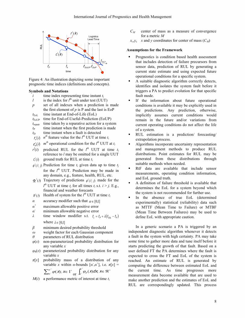
Figure 4: An illustration depicting some important prognostic time indices (definitions and concepts).

Symbols and Notations i time index representing time instant ti l is the index for lth unit under test (UUT) p set of all indexes when a prediction is made

the first element of p is P and the last is EoP tEoL time instant at EndofLife (EoL) tEoUP time for EndofUsefulPrediction (EoUP) trepair time taken by a reparative action for a system tP time instant when the first prediction is made tD time instant when a fault is detected

if ln nth feature value for the lth UUT at time ti

ic lm mth operational condition for the lth UUT at ti

rl(i) predicted RUL for the lth UUT at time ti reference to l may be omitted for a single UUT

)(* ir l ground truth for RUL at time ti )|( jil Prediction for time ti given data up to time tj for the lth UUT. Prediction may be made in any domain, e.g., feature, health, RUL, etc.

)(il Trajectory of predictions )|( jil made for the lth UUT at time tj for all times ti s.t. i > j. E.g., financial and weather forecasts

)(ihl Health of system for the lth UUT at time ti α accuracy modifier such that ]1,0[ α+ maximum allowable positive error α minimum allowable negative error λ time window modifier s.t. PEoLP tttt

where ]1,0[ β minimum desired probability threshold ω weight factor for each Gaussian component θ parameters of RUL distribution φ(x) nonparameterized probability distribution for

any variable x φθ(x) parameterized probability distribution for any

variable x π[x] probability mass of a distribution of any

variable x within αbounds [α,α+], i.e. π[x] =

Ι;)( xx

or

xdxx ;)(

M(i) a performance metric of interest at time ti

CM center of mass as a measure of convergence for a metric M

xc,yc x and y coordinates for center of mass (CM)

Assumptions for the Framework

Prognostics is condition based health assessment that includes detection of failure precursors from sensor data, prediction of RUL by generating a current state estimate and using expected future operational conditions for a specific system.

A suitable diagnostic algorithm correctly detects, identifies and isolates the system fault before it triggers a PA to predict evolution for that specific fault mode.

If the information about future operational conditions is available it may be explicitly used in the predictions. Any prediction, otherwise, implicitly assumes current conditions would remain in the future and/or variations from current operating conditions do not affect the life of a system.

RUL estimation is a prediction/ forecasting/ extrapolation process.

Algorithms incorporate uncertainty representation and management methods to produce RUL distributions. Point estimates for RUL may be generated from these distributions through suitable methods when needed.

RtF data are available that include sensor measurements, operating condition information, and EoL ground truth.

A definition of failure threshold is available that determines the EoL for a system beyond which the system is not recommended for further use.

In the absence of true EoL (determined experimentally) statistical (reliability) data such as MTTF (Mean Time to Failure) or MTBF (Mean Time Between Failures) may be used to define EoL with appropriate caution.

In a generic scenario a PA is triggered by an

independent diagnostic algorithm whenever it detects a fault in the system with high certainty. PA may take some time to gather more data and tune itself before it starts predicting the growth of that fault. Based on a user defined FT the PA determines where the fault is expected to cross the FT and EoL of the system is reached. An estimate of RUL is generated by computing the difference between estimated EoL and the current time. As time progresses more measurement data become available that are used to make another prediction and the estimates of EoL and RUL are correspondingly updated. This process


9

continues until one of the following happens: the system is taken down for maintenance. EoUP is reached and any further predictions may

not be useful for failure avoidance operations. the system has failed (unexpectedly). the case where problem symptoms have

disappeared (can occur if there were false alarms, intermittent fault, etc.).

Definitions

Time Index: In a prognostics application time can be discrete or continuous. A time index i will be used instead of the actual time, e.g., i=10 means t10. This takes care of cases where sampling time is not uniform. Furthermore, time indexes are invariant to time-scales.

Time of Detection of F ault: Let D be the time index for time (tD) at which the diagnostic or fault detection algorithm detected the fault. This process will trigger the prognostics algorithm which should start making RUL predictions as soon as enough data has been collected, usually shortly after the fault was detected. For some applications, there may not be an explicit declaration of fault detection, e.g., applications like battery health management, where prognosis is carried out on a decay process. For such applications tD can be considered equal to t0 i.e., prognostics is expected to trigger as soon as enough data has been collected instead of waiting for an explicit diagnostic flag (see Figure 5).

Time to Start Prediction: Time indices for times at which a fault is detected (tD) and when the system starts predicting (tP) are differentiated. For certain algorithms tD = tP but in general tP ≥ tD as PAs need some time to tune with additional fault progression data before they can start making predictions (Figure 5). Cases where a continuous data collection system is employed even before a fault is detected, sufficient data may already be available to start making predictions and hence tP = tD.

Prognostics F eatures: Let )(if ln

be a feature at time index i, where n = 1, 2, …, N is the feature index, and l = 1, 2, … , L is the UUT index (an index identifying the different units under test). In prognostics, irrespective of the analysis domain, i.e., time, frequency, wavelet, etc., features take the form of time series and can be physical variables, system parameters or any other quantity that can be computed from observable variables of the system to provide or aid prognosis. Features can be also referred to as a 1xN feature vector F l(i) of the lth UUT at time index i.

Operational Conditions: Let )(ic lm

be an operational condition at time index i, where m = 1, 2, … , M is the condition index, and l = 1, 2, … , L is the UUT index.

Operational conditions describe how the system is being operated and also include the load on the system. The conditions can also be referred to as a 1xM vector Cl(i) of the lth UUT at time index i. The matrix Cl for all times < tP is referred to as load history and for times ≥ tP as operational (load) profile for the system.

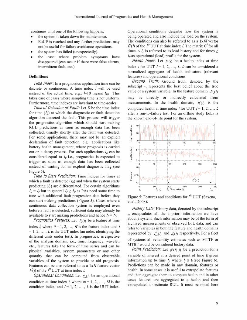
H ealth Index: Let )(ihl be a health index at time index i for UUT l = 1, 2, …, L. h can be considered a normalized aggregate of health indicators (relevant features) and operational conditions.

Ground Truth: Ground truth, denoted by the subscript *, represents the best belief about the true value of a system variable. In the feature domain )(* if l

n

may be directly or indirectly calculated from measurements. In the health domain, )(* ihl is the computed health at time index i for UUT l = 1, 2, …, L after a run-to-failure test. For an offline study EoL* is the known end-of-life point for the system.

0 50 100 150 200 250552

554

556

Feat

ure

1

0 50 100 150 200 2500

20

40

Cond

ition

1

0 50 100 150 200 25047

47.5

48

Time Index (i)

Feat

ure

2

Pt0t EoLtFt

)(* Pr l

Dt

Hea

lth In

dex

Feat

ure

0

1

Load

con

ditio

n

Figure 5: Features and conditions for lth UUT (Saxena, et al., 2008).

History Data: History data, denoted by the subscript #, encapsulates all the a priori information we have about a system. Such information may be of the form of archived measurements or observed EoL data, and can refer to variables in both the feature and health domains represented by )(# if l

n and )(# ihl respectively. For a fleet

of systems all reliability estimates such as MTTF or MTBF would be considered history data.

Point Prediction: Let )|( jil be a prediction for a variable of interest at a desired point of time tj given information up to time tj, where tj ≤ ti (see Figure 6). Predictions can be made in any domain, features or health. In some cases it is useful to extrapolate features and then aggregate them to compute health and in other cases features are aggregated to a health and then extrapolated to estimate RUL. It must be noted here


10

that a point prediction may be expressed as probability a distribution or estimated moments derived from the probability distribution.

Trajectory Prediction: Let )(il be a trajectory of predictions formed by point predictions for a variable of interest from time index i onwards such that

)(il = )|(),...,|1(),|( iEoPiiii lll (see Figure 6). It must be noted that only the last point of this trajectory, i.e., )|( iEoPl is used to estimate RUL.

itDtFt)( irt

)|( iil)|1( iil

)|( iEoPl

Pred

icte

d Va

riabl

e

Pt

Failure Threshold

Time

)(ir l

Figure 6: Illustration showing a trajectory prediction. Predictions get updated every time instant.

RUL: Let )(ir l be the remaining useful life estimate at time index i given that the information (features and conditions) up to time index i and an expected operational profile for the future are available. RUL is computed as the difference between the predicted time of failure (where health index approaches zero) and the current time ti. RUL is estimated as

ijl ttir )( , where izzhj l

z ,0)(max . (1)

Corresponding ground truth is computed as izzhjttir l

zzij

l ,0)(maxwhere,)( **. (2)

RUL vs. Time Plot: RUL values are plotted against time to compare with RUL ground truth (represented by a straight line). As illustrated in Figure 7, this visually summarizes prediction performance as it evolves through time. This plot is the foundation of prognostic metrics developed in subsequent sections.

0 50 100 150 200 2500

50

100

150

200

Time Index (i)

RUL(

i)

RUL* Plotted with Time

D P EoLF

)125(lr

)100(lr )200(lr

)150(lr

time index Figure 7: Comparing RUL predictions from ground truth ( ]240,70[| PPp , tEoL = 240, tEoP > 240) (Saxena, et al., 2008).

5.1 Incorporating Uncertainty Estimates As discussed in section 4, prognostics is meaningless unless the uncertainties in the predictions are accounted for. PAs can handle these uncertainties in various ways such as propagating through time the prior probabilities of uncertain inputs and estimating posteriori distributions of EoL and RUL quantities (Orchard & Vachtsevanos, 2009). Therefore, the metrics should be designed such that they can make use of these distributions while assessing the performance. The first step in doing so is to define a reasonable point estimate from these distributions such that no interesting features get ignored in decision making. Computationally the simplest, and hence most widely used, practice has been to compute mean and variance estimates of these distributions (Goebel, Saha, & Saxena, 2008). In reality these distributions are rarely smooth or symmetric, thereby resulting in large errors due to such simplifying assumptions especially while carrying out performance assessment. It is, therefore, suggested that other estimates of central tendency (location) and variance (spread) be used instead of mean and standard deviation, which are appropriate only for Normal cases. For situations were normality of the distribution cannot be established, it is preferable to rely on median as a measure of location and the quartiles or Inter Quartile Range (IQR) as a measure of spread (Hoaglin, Mosteller, & Tukey, 1983). Various types of distributions are categorized into four categories and corresponding methods to compute more appropriate location and spread measures are suggested in Table 3. For the purpose of plotting and visualizing the data use of error bars and boxplots is suggested (Figure 8); more explanation is given in the following sections.

+95% bound

outliers

25% quartile

50% quartile

-95% bound

1 32

1 2 3

Normal

Figure 8: Visual representation for distributions. Distributions shown on the left can be represented by box plots as shown on the right (Saxena, et al., 2009b).

While mean and variance estimates are good for easy understanding they can be less robust when deviations from assumed distribution category are


11

random and frequent. Furthermore, given the fact that there will be uncertainty in any prediction one must make provisions to account for these deviations. One common way to do so is to specify an allowable error bound around the point of interest and one could use the total probability of failure within that error bound instead of basing a decision on a single point estimate. As shown in Figure 9, this error bound may be asymmetric especially in the case of prognostics, since it is often argued that an early prediction is preferred over a late prediction.

][EoL

*EoLEoL

Predicted EoL Distribution

EoL Point Estimate

EoL Ground Truth

Total Probability of EoL within α-bounds

Asymmetricα-bounds

Figure 9: Concepts for incorporating uncertainties.

These ideas can be analytically incorporated into the numerical aspect of the metrics by computing the probability mass of a prediction falling within the specified αbounds. As illustrated in the figure, the EoL ground truth may be very different than the estimated EoL and hence the decisions based on probability mass are expectedly more robust. Computing the probability mass requires integrating the probability distribution between the αbounds (Figure 10). The cases where analytical form of the distribution is available, like for Normal distributions, this probability mass can be computed analytically by integrating the area under the prediction PDF between the αbounds (α to α+). However, for cases where there is no analytical form available, a summation based on histogram obtained from the process/algorithm can be used to compute this probability (see Figure 10). A formal way to include this probability mass into the analytical framework is by introducing a βcriterion, where a prediction is considered inside αbounds only if the probability mass of the corresponding distribution within the αbounds is more than a predetermined threshold β. This parameter is also linked to the issues of uncertainty management and risk absorbing capacity of the system.

Known Distribution ?

Obtain RUL distribution

Estimate parameters (θ)

kernel smoothing

Integrate the PDF between α-bounds to

obtain total probability

Sum samples in the pdf histogram that

fall within α-bounds

Analyze RUL distribution

Op t iona l

Y N

Total probability of RUL between α-bounds

Identified with a known parametric

distribution

Classify as a non-parametric

distribution

Analytical form of PDF

Probability Histogram

Ι;)( xx

][EoL

][EoL

xdxx ;)(

Figure 10: Procedure to compute probability mass of RULs falling within specified αbounds.

The categorization shown in Table 3 determines the method of computing the probability of RULs falling between αbounds, i.e., area integration or discrete summation, as well as how to represent it visually. For cases that involve a Normal distribution, using a confidence interval represented by a confidence bar around the point prediction is sufficient (Devore, 2004). For situations with nonNormal single mode distributions this can be done with an interquartile plot represented by a box plot (Martinez, 2004). Box plots convey how a prediction distribution is skewed and whether this skew should be considered while computing a metric. A box plot also has provisions to represent outliers, which may be useful to keep track of in risk sensitive situations. It is suggested to use box plots superimposed with a dot representing the mean of the distribution. This will allow keeping the visual information in perspective with respect to the conventional plots. For the mixture of Gaussians case, it is recommended that a model with few (preferably n ≤ 4) Gaussian modes is created and corresponding confidence bars plotted adjacent to each other. The


12

weights for each Gaussian component can then be represented by the thickness of the error bars. It is not recommended to plot multiple box plots since there is no methodical way to differentiate and isolate the samples associated to individual Gaussian components, and compute the quartile ranges separately for each of them. A linear additive model is assumed here for simplicity while computing the mixture of Gaussians.

InNNx nnn );,(...),()( 111 (3)

where: )(x is a PDF with of multiple Gaussians

ω is the weight factor for each Gaussian component N(µ, σ) is a Gaussian distribution with parameters µ and σ n is the number of Gaussian modes identified in the distribution.

Table 3: Methodology to select location and spread measures along with visualization methods (Saxena, et al., 2009b).

Normal D istribution Mixture of Gaussians Non-Normal D istribution

Multimodal(non-Normal)

Parametric Non-Parametric

Location(Central tendency) Mean (µ) Means: µ1, µ2, …, µn

weights: ω1, ω 2, …, ωn

Mean, Median,L-estimator,M-estimator

Dominant median, Multiple medians,L-estimator,M-estimator

Spread(variability)

Sample standard deviation (σ),IQR (inter quartile range)

Sample standard deviations:σ 1, σ 2, …, σ n

Mean Absolute Deviation (MAD) ,Median Absolute Deviation (MdAD) ,Bootstrap methods , IQR

Visualization

Confidence Interval (CI),Box plot with mean

Multiple CIs with varying bar width

Note: here ω1 > ω 2 > ω 3

Box plot with mean Box plot with mean

1

22

33

1

6. PERFORMANCE METRICS

6.1 Limitations of Classical Metrics In Saxena, et al. (2009a) it was reported that the most commonly used metrics in the forecasting applications are accuracy (bias), precision (spread), MSE, and MAPE. Tracking the evolution of these metrics one can see that these metrics were successively developed to incorporate issues not covered by their predecessors. There are more variations and modifications that can be found in literature that measure different aspects of performance. Although these metrics captured important aspects, this paper focuses on enumerating various shortcomings of these metrics from a prognostics viewpoint. Researchers in the PHM community have further adapted these metrics to tackle

these shortcomings in many ways (Saxena, et al., 2008). However, there are some fundamental differences between the performance requirements from general forecasting applications and prognostics applications that did not get adequately addressed. This translates into differences at the design level for the metrics in either case. Some of these differences are discussed here. These metrics provide a statistical accounting of variations in the distribution of RULs. Whereas this is meaningful information, these metrics are not designed for applications where RULs are continuously updated as more data becomes available. Prognostics prediction performance (e.g., accuracy and precision) tends to be more critical as time passes by and the system nears its endoflife. Considering EoL as a fixed reference point in time, predictions made at different times create


13

several conceptual difficulties in computing an aggregate measure using conventional metrics. Predictions made early on have access to less information about the dynamics of fault evolution and are required to predict farther in time. This makes the prediction task more difficult as compared to predicting at a later stage. Each successive prediction utilizes additional data available to it. Therefore, a simple aggregate of performance over multiple predictions made is not a fair representative of overall performance. It may be reasonable to aggregate fixed nstep ahead (fixed horizon) predictions instead of aggregating EoL predictions (moving horizon). Performance at specific times relative to the EoL can be a reasonable alternative as well. Furthermore, most physical processes describing fault evolution tend to be more or less monotonic in nature. In such cases it becomes easier to learn true parameters of the process as more data become available. Thus, it may be equally important to quantify how well and how quickly an algorithm improves as more data become available. Following from the previous argument, conventional measures of accuracy and precision tend to account for statistical bias and spread arising from the system. What is missing from the prognostics point of view is a measure that encapsulates the notion of performance improvement with time, since prognostics continuously updates, i.e., successive predictions occur at early stages close to fault detection, middle stages while the fault evolves, and late stages nearing EoL. Depending on application scenarios, criticality of predictions at different stages may be ranked differently. A robust metric should be capable of making an assessment at all stages. This will not only allow ranking various algorithms at different stages but also allow switching prediction models with evolving fault stages instead of using a single prediction algorithm until EoL. Time scales involved in prognostics applications vary widely (on the order of seconds and minutes for electronic components vs. weeks and years for battery packs). This raises an important question “how far in advance is enough when predicting with a desired confidence?” Although the earlier the better, a sufficient time to plan and carry out an appropriate corrective action is what is sought. While qualitatively these performance measures remain the same (i.e., accuracy and precision) one needs to incorporate the issues of time criticality. The new metrics developed and discussed in the following sections attempt to alleviate some of these issues in evaluating prognostic performance.

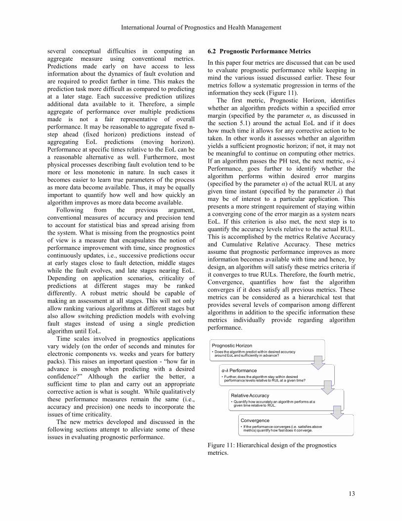
6.2 Prognostic Performance Metrics In this paper four metrics are discussed that can be used to evaluate prognostic performance while keeping in mind the various issued discussed earlier. These four metrics follow a systematic progression in terms of the information they seek (Figure 11). The first metric, Prognostic Horizon, identifies whether an algorithm predicts within a specified error margin (specified by the parameter α, as discussed in the section 5.1) around the actual EoL and if it does how much time it allows for any corrective action to be taken. In other words it assesses whether an algorithm yields a sufficient prognostic horizon; if not, it may not be meaningful to continue on computing other metrics. If an algorithm passes the PH test, the next metric, αλ Performance, goes further to identify whether the algorithm performs within desired error margins (specified by the parameter α) of the actual RUL at any given time instant (specified by the parameter λ) that may be of interest to a particular application. This presents a more stringent requirement of staying within a converging cone of the error margin as a system nears EoL. If this criterion is also met, the next step is to quantify the accuracy levels relative to the actual RUL. This is accomplished by the metrics Relative Accuracy and Cumulative Relative Accuracy. These metrics assume that prognostic performance improves as more information becomes available with time and hence, by design, an algorithm will satisfy these metrics criteria if it converges to true RULs. Therefore, the fourth metric, Convergence, quantifies how fast the algorithm converges if it does satisfy all previous metrics. These metrics can be considered as a hierarchical test that provides several levels of comparison among different algorithms in addition to the specific information these metrics individually provide regarding algorithm performance.

Prognostic Horizon• Does the algorithm predict within desired accuracy

around EoLand sufficiently in advance?

α-λ Performance• Further, does the algorithm stay within desired

performance levels relative to RUL at a given time?

Relative Accuracy• Quantify how accurately an algorithm performs at a

given time relative to RUL.

Convergence• If the performance converges (i.e. satisfies above

metrics) quantify how fast does it converge.

Figure 11: Hierarchical design of the prognostics metrics.


14

It must be noted that these metrics share the attribute of performance tracking with time unlike the classical metrics. Discussion on detailed definitions and descriptions of these metrics follows henceforth.

Prognostic Horizon: Prognostic Horizon (PH) is defined as the difference between the time index i when the predictions first meet the specified performance criteria (based on data accumulated until time index i) and the time index for EoL. The performance requirement may be specified in terms of an allowable error bound (α) around the true EoL. The choice of α depends on the estimate of time required to take a corrective action. Depending on the situation this corrective action may correspond to performing maintenance (manufacturing plants) or bringing the system to a safe operating mode (operations in a combat zone).

iEoL ttPH (4)

where:

)(|min jrpjji is the first time

index when predictions satisfy β-criterion for a given α

p is the set of all time indexes when predictions are made

l is the index for lth unit under test (UUT)

β is the minimum acceptable probability mass

r(j) is the predicted RUL distribution at time tj

tEoL is the predicted End-of-Life

)( jr is the probability mass of the prediction PDF within the α-bounds that are given by

EoLEoL trtr ** and

As shown in Figure 12, the desired level of accuracy with respect to the EoL ground truth is specified as ±αbounds (shaded band). RUL distributions are then plotted against time for all the algorithms that are to be compared. In simple cases the evaluation may be based on point estimates (mean, median, etc.) of the distributions. The PH for an algorithm is declared as soon the corresponding prediction enters the band of desired accuracy. As is evident from the illustration in Figure 12(a), the second algorithm (A2) has a longer PH. However, looking closely at the plots, A1 does not perform much worse than A2, but this method, being less robust due to use of only a point estimate, results in very different PH values for the two algorithms. This can be improved by using the βcriterion, as shown in Figure 12(b).

(a)

1PH

*EoL'k

RU

L

2PH

*EoLk

RU

L

time

)]([ kr

1PH

(b)

Figure 12: (a) Illustration of Prognostics Horizon while comparing two algorithms based on point estimates (distribution means) (b) PH based on βcriterion results in a more robust metric.

Prognostic horizon produces a score that depends on length of ailing life of a system and the time scales in the problem at hand. The range of PH is between (tEoLtP) and max0, tEoLtEoP. The best score for PH is obtained when an algorithm always predicts within desired accuracy zone and the worst score when it never predicts within the accuracy zone. The notion for Prediction Horizon has been long discussed in the literature from a conceptual point of view. This metric indicates whether the predicted estimates are within specified limits around the actual EoL so that the predictions are considered trustworthy. It is clear that a longer prognostic horizon results in more time available to act based on a prediction that has some desired credibility. Therefore, when comparing algorithms, an algorithm with longer prediction horizon would be preferred. αλ Performance: This metric quantifies prediction quality by determining whether the prediction falls within specified limits at particular times with respect to a performance measure. These time instances may be specified as percentage of total ailing life of the system. The discussion henceforth is presented in the context of


15

accuracy as a performance measure, hence αλ accuracy, but any performance measure of interest may fit in this framework. αλ accuracy is defined as a binary metric that evaluates whether the prediction accuracy at specific time instance tλ falls within specified αbounds (Figure 13). Here tλ is a fraction of time between tP and the actual tEoL. The αbounds here are expressed as a percentage of actual RUL r(iλ) at tλ.

otherwise0)(if1

irAccuracy (5)

where:

λ is the time window modifier such that )( PEoLP tttt

β is the minimum acceptable probability for β-criterion

r(iλ) is the predicted RUL at time index iλ

)(ir is the probability mass of the prediction PDF within the α-bounds that are given by

)()(and)()( ** iriririr

EoL2t

Δ(R

UL

erro

r)

time

)]([ kr

1t

0

(b)

EoL2t

RU

L

time

)]([ kr

1t

(a)

Figure 13: (a) αλ accuracy with the accuracy cone shrinking with time on RUL vs. time plot. (b) Alternate representation of αλ accuracy on RULerror vs. time plot.

As an example, this metric would determine whether a prediction falls within 10% accuracy (α = 0.1) of the true RUL halfway to failure from the time the first prediction is made (λ = 0.5). The output of this metric is binary (1=Yes or 0=No) stating whether the

desired condition is met at a particular time. This is a more stringent requirement as compared to prediction horizon, as it requires predictions to stay within a cone of accuracy i.e., the bounds that shrink as time passes by as shown in Figure 13(a). For easier interpretability αλ accuracy can also be plotted as shown in Figure 13(b). It must be noted that the set of all time indexes (p) where a prediction is made is determined by the frequency of prediction step in a PA. Therefore, it is possible that for a given λ there is no prediction assessed at time tλ if the corresponding pi . In such cases one can make alternative arrangements such as choosing another λ’ closest to λ such that pi ' . Relative Accuracy: Relative Accuracy (RA) is defined as a measure of error in RUL prediction relative to the actual RUL r*(iλ) at a specific time index iλ.

ir

irirRA l

ll

l

*

*1

(6)

where:

λ is the time window modifier such that )( PEoLP tttt

,

l is the index for lth unit under test (UUT),

r*(iλ) is the ground truth RUL at time index iλ,

)( ir is an appropriate central tendency point estimate of the predicted RUL distribution at time index iλ.

This is a notion similar to αλ accuracy where, instead of finding out whether the predictions fall within a given accuracy level at a given time instant, accuracy is measured quantitatively (see Figure 14). First a suitable central tendency point estimate is obtained from the prediction probability distribution using guidelines provided in Table 3 and then using Eq.6.

1

RU

L

timePt EOLtt

2Point Estimate (Median)Distribution Mean

Δ1

Δ2

Figure 14: Schematic illustrating Relative Accuracy.


16

RA may be computed at a desired time tλ. For cases with mixture of Gaussians a weighted aggregate of the means of individual modes can be used as the point estimate; where the weighting function is the same as the one for the various Gaussian components in the distribution. An algorithm with higher relative accuracy is desirable. The range of values for RA is [0,1], where the perfect score is 1. It must be noted that if the prediction error magnitude grows beyond 100%, RA results in a negative value. Large errors like these, if interpreted in terms of α parameter for previous metrics, would correspond to values greater than 1. Cases like these need not be considered as it is expected that, under reasonable assumptions, preferred α values will be less than 1 for PH and αλ accuracy metrics and that these cases would not have met those criteria anyway. RA conveys information at a specific time. It can be evaluated at multiple time instances before tλ to account for general behavior of the algorithm over time. To aggregate these accuracy levels, Cumulative Relative Accuracy (CRA) can be defined as a normalized weighted sum of relative accuracies at specific time instances.

pi

lll RAirwp

CRA 1 (7)

where:

w(rl(i)) is a weight factor as a function of RUL at all time indices

p is the set of all time indexes before tλ when a prediction is made

p is the cardinality of the set

In most cases it is desirable to weigh those relative accuracies higher that are closer to tEoL. In general, it is expected that tλ is chosen such that it holds some physical significance such as a time index that provides a required prediction horizon, or time required to apply a corrective action, etc. For instance, RA evaluated at t0.5 signifies the time when a system is expected to have consumed half of its ailing life, or in terms of damage index the time index when damage magnitude has reached 50% of the failure threshold. This metric is useful in comparing different algorithms for a given λ in order to get an idea on how well a particular algorithm does at significant times. Choice of tλ should also take into account the uncertainty levels that an algorithm entails by making sure that the distribution spread at tλ does not cross over expected tEoL by significant margins especially for critical applications. In other words the probability mass of the RUL

distribution at tλ extending beyond EoL should not be too large. Convergence: Convergence is a metametric defined to quantify the rate at which any metric (M) like accuracy or precision improves with time. It is defined as the distance between the origin and the centroid of the area under the curve for a metric is a measure of convergence rate.

,)( 22cPcM ytxC (8)

where:

CM is the Euclidean distance between the center of mass (xc, yc) and (tP, 0)

M(i) is a non-negative prediction accuracy or precision metric with a time varying value

(xc, yc) is the center of mass of the area under the curve M(i) between tP and tEoUP, defined as following

.)()(

)()(21

y

and ,)()(

)()(21

x

1

21

c

1

221

c

EoUP

Piii

EoUP

Piii

EoUP

Piii

EoUP

Piii

iMtt

iMtt

iMtt

iMtt

(9)

As suggested earlier, this discussion assumes that the algorithm performance improves with time. This is easily established if it has passed criteria for previous metrics. For illustration of the concept in Figure 15 three cases are shown that converge at different rates. Lower distance means a faster convergence. Convergence is a useful metric since we expect a prognostics algorithm to converge to the true value as more information accumulates over time. Further, a faster convergence is desired to achieve a high confidence in keeping the prediction horizon as large as possible.

Point Estimate of Metric value

Per

form

ance

Mea

sure

(M)

timePt EoLt

EoPt

1,cx

1,cy 3,MC2,MC1

2

3

3,2,1, MMM CCC

EoUPt

Center of Mass

Figure 15: Convergence compares the rates at which different algorithms improve.


17

6.2.1 Applying the Prognostics Metrics In practice, there can be several situations where the definitions discussed above result in ambiguity. In Saxena, et al. (2009a) several such situations have been discussed in detail with corresponding suggested resolutions. For the sake of completeness such situations are very briefly discussed here. With regards to PH metric, the most common situation encountered is when the RUL trajectory jumps out of the ±α accuracy bounds temporarily. Situations like this result in multiple time indexes where RUL trajectory enters the accuracy zone to satisfy the metric criteria. A simple and conservative approach to deal with this situation is to declare a PH at the latest time instant the predictions enter accuracy zone. Another option is to use the original PH definition and further evaluate other metrics to determine whether the algorithm satisfies all other requirements. Situations like these can occur due to a variety of reasons.

Inadequate system model: Real systems often exhibit inherent transients at different stages during their life cycles. These transients get reflected as deviations in computed RUL estimates from the true value if the underlying model assumed for the system does not account for these behaviors. In such cases, one must step back and refine the respective models to incorporate such dynamics.

Operational transients: Another source of such behaviors can be due to sudden changes in operational profiles under which a system is operating. Prognostic algorithms may show a time lag in adapting to such changes and hence resulting in temporary deviation from the real values.

Uncertainties in prognostic environments: Prognostics models a stochastic process and hence the behavior observed from a particular run (single realization of the stochastic process) may not exhibit the true nature of prediction trajectories. Assuming that all possible measures for uncertainty reduction have been taken during algorithm development, such observations should be treated as isolated realization of the process. In that case these trajectories should be aggregated from multiple runs to achieve statistical significance or more sophisticated stochastic analyses can be carried out.

Plotting the RUL trajectory in the PH plot provides insights for such deficiencies to algorithm developers. It is important to identify the correct reason before computing a metric and interpreting its result. Ideally, an algorithm and a system model should be robust to transients inherent to the system behavior and operational conditions.

The situations discussed above are more common towards the end when a system nears EoL. This is because in most cases the fault evolution dynamics are too fast and complex to model or learn from data as the system nears EoL. Therefore, RUL curve deviates from the error band near tEoL. To determine whether such deviations are critical for postprognostic decision making, the concept of tEoUP or EndofUsefulPredictions (EoUP) is introduced. This index represents the minimum allowable PH that is required to take a corrective measure. Any predictions made beyond EoUP are of little or no use from a practical viewpoint.

6.2.2 Choosing Performance Parameters From a topdown perspective, the main idea behind these metrics is to help management generate appropriate specifications and requirements for prognostics algorithm in fielded applications. The outcome of these metrics depends directly on the values chosen for input parameters like α, λ, and β. Thus, the choice of values for these parameters forms an important aspect of performance evaluation and interpretation. Costbenefitrisk analyses are generally performed through various methods that model the effects of a variety of constraints (financial costs, safety, criticality of mission completion, reputation, etc.) and derive a range of available slacks in achieving an overall benefit situation (pareto optimal solutions). It is expected that the parameters can be incorporated in these analyses to include the effects of prognostic performance on the costbenefit of PHM. While this subject is out of the scope of this paper a brief discussion is provided for an overall perspective on how these parameters can be connected to safety, logistics and cost constraints. There are systems that involve different levels of criticality when they fail. In a mission critical scenario a failure may be catastrophic and hence a limited number of false positives may be tolerable but no false negatives. In other cases the cost of acting on false positives may be prohibitively high. There are cases where it is more cost effective to tolerate several false negatives as opposed to reacting to a false positive and hence it is acceptable even if the system runs to failure once in a while. There are several factors that determine how critical it may be to make a correct prediction. These factors combined together should dictate the choice of these parameters while carrying out performance evaluation. Some of the most important factors are: Time for problem mitigation: the amount of time to

mitigate a problem or start a corrective action when critical health deterioration of a component/system has been detected is a very important factor. As mentioned earlier, very


18

accurate predictions at a time when no recovery action can be made are not useful. Hence, a tradeoff between error tolerance and time for recovery from fault should be considered. The time for problem mitigation will vary from system to system and involves multiple factors. This factor will have a direct consequence on λ parameter.

Cost of mitigation: cost of the reparative action is an important factor in all management related decisions and hence should be considered. From a decision making point of view this can be associated to the cost due to false positives. This factor influences α, where there is often a tradeoff between false positives and true positive rates.

Criticality of system or cost of failure: This quantifies the effect of false negatives. Further, while comparing timecritical scenarios, resources should be directed towards more critical and important components in order to efficiently maintain overall health of the system. Likewise, if the health assessment is being performed on multiple units in a system, the parameters for different units should be chosen based on a prioritized list of criticality. Assessment of criticality is usually done based on severity and frequency of occurrence statistics available from Failure Modes, Effects, and Criticality Analysis (FMECA) studies (MILSTD1629A, 1980). Another perspective to assess criticality is based on costbenefit analysis where cost of failures is incorporated to assess the implications of false negatives (Banks & Merenich, 2007; Feldman, et al., 2008).

Uncertainty management capability: Level of confidence on the uncertainty management capability and costs of system failure determine the risk absorbing capacity in a particular scenario. The choice of β is guided by such factors.

Note that these factors mentioned here are not arranged based on any order of importance; users should consider them based on the characteristics of their systems and may skip a few as appropriate.

7. FUTURE WORK

A natural extension of this work leads into the development of online prognostic performance metrics. This would require investigations into several issues that were set aside through various assumptions in the present work. For instance, thus far performance evaluation ignores the effect of future loading conditions that alter the rate of remaining life consumption. Performance evaluation without an explicit knowledge about EoL is a challenge for online metrics. These metrics will also need to include provisions for the effects of scheduled maintenance and

selfhealing characteristics in some systems. Further, the concepts presented in this paper will be refined and applied to a variety of applications. Developing more metrics like robustness and sensitivity, etc. also remains on the research agenda. Finally, a formal framework for connecting these metrics to top level requirements through development of uncertainty management and representation (URM) methods, incorporation of risk analysis, costbenefit analysis, and requirements flow down remains a topic of interest in future work.

8. CONCLUSION

This paper presents several performance metrics for offline evaluation of prognostics algorithms. A brief overview of different methods employed for performance evaluation is also included. It has been shown that various forecasting related applications differ from prognostics in the systems health management context. This called for developing specialized metrics for prognostics. These metrics were developed keeping in mind various critical aspects that must be included in performance evaluation. A formal prognostic framework was presented to clearly define the concepts and introduce the terminology. Metrics with uncertainty representation capabilities were developed that track the performance of an algorithm with time. Along with detailed discussions and illustrations, it has been shown that these metrics can be successfully applied to evaluate prognostic performance in a standardized manner. Furthermore, it has been discussed that the suggested metrics can be employed to reflect high level requirements in a practical PHM system.

A C K N O W L E D G M E N T

The authors would like to express their gratitude to colleagues at the Prognostic Center of Excellence (NASA Ames Research Center) and external partners at Impact Technologies and Clarkson University for participating in research discussions, evaluating metrics in their respective applications, and providing a valuable feedback. This work was funded by NASA Aviation Safety ProgramIVHM Project.

R E F E R E N C ES

Banks, J., & Merenich, J. (2007). Cost benefit analysis for asset health management technology. Reliability and Maintainability Symposium (RAMS), Orlando, FL.

Carrasco, M., & Cassady, C. R. (2006, 2326 Jan. 2006). A study of the impact of prognostic errors on system performance. Annual Reliability and Maintainability Symposium, RAMS06.

Coble, J. B., & Hines, J. W. (2008). Prognostic Algorithm Categorization with PHM Challenge


19

Application. 1st International Conference on Prognostics and Health Management (PHM08), Denver, CO.

Coppe, A., Haftka, R. T., Kim, N., & Yuan, F. (2009). Reducing Uncertainty in Damage Growth Properties by Structural Health Monitoring. Annual Conference of the Prognostics and Health Management Society (PHM09) San Diego, CA.

DeNeufville, R. (2004). Uncertainty Management for Engineering Systems Planning and Design. Engineering Systems Symposium MIT, Cambridge, MA.

Devore, J. L. (2004). Probability and Statistics for Engineering and the Sciences (6th ed.): Thomson.

Drummond, C., & Yang, C. (2008). Reverse Engineering Costs: How Much will a Prognostic Algorithm Save? International Conference on Prognostics and Health Management, Denver, CO.

Engel, S. J. (2008, October 69, 2008). Prognosis Requirements and V&V: Panel Discussion on PHM Capabilities: Verification, Validation, and Certification Issues. International Conference on Prognostics and Health Management (PHM08), Denver, CO.

Engel, S. J., Gilmartin, B. J., Bongort, K., & Hess, A. (2000). Prognostics, the Real Issues Involved with Predicting Life Remaining. IEEE Aerospace Conference, Big Sky, MT.

Feldman, K., Sandborn, P., & Jazouli, T. (2008). The Analysis of Return on Investment for PHM Applied to Electronic Systems. International Conference on Prognostics and Health Management (PHM08), Denver, CO.

Goebel, K., & Bonissone, P. (2005). Prognostic Information Fusion for Constant Load Systems. 7th Annual Conference on Information Fusion.

Goebel, K., Saha, B., & Saxena, A. (2008). A Comparison of Three DataDriven Techniques for Prognostics. 62nd Meeting of the Society For Machinery Failure Prevention Technology (MFPT), Virginia Beach, VA.

Guan, X., Liu, Y., Saxena, A., Celaya, J., & Goebel, K. (2009). EntropyBased Probabilistic Fatigue Damage Prognosis and Algorithmic Performance Comparison. Annual Conference of the Prognostics and Health Management Society (PHM09), San Diego, CA.

Hastings, D., & McManus, H. (2004). A Framework for Understanding Uncertainty and its Mitigation and Exploitation in Complex Systems. Engineering Systems Symposium MIT, Cambridge MA.

Hoaglin, D. C., Mosteller, F., & Tukey, J. W. (Eds.). (1983). Understanding Robust and Exploratory Data Analysis: John Wiley & Sons.

Condition Monitoring and Diagnostics of Machines Prognostics part 1: General Guidelines, ISO/IEC Directives Part 2 C.F.R. (2004).

Leao, B. P., Yoneyama, T., Rocha, G. C., & Fitzgibbon, K. T. (2008). Prognostics Performance Metrics and Their Relation to Requirements, Design, Verification and CostBenefit. International Conference on Prognostics and Health Management (PHM08), Denver CO.

Martinez, A. R. (2004). Exploratory Data Analysis with MATLAB. In A. R. Martinez (Ed.): CRC Press.

MILSTD1629A. (1980). Military Standard: Procedures for Performing A Failure Mode, Effects and Criticality Analysis. Washington DC: Department of Defense.

NASA. (2009). NASA Aviation Safety Program Retrieved December 2009, from http://www.aeronautics.nasa.gov/programs_avsafe.htm

Ng, K.C., & Abramson, B. (1990). Uncertainty Management in Expert Systems. IEEE Expert Systems, 5, 20.

Orchard, M., Kacprzynski, G., Goebel, K., Saha, B., & Vachtsevanos, G. (2008). Advances in Uncertainty Representation and Management for Particle Filtering Applied to Prognostics. International Conference on Prognostics and Health Management (PHM08), Denver, CO.

Orchard, M. E., Tang, L., Goebel, K., & Vachtsevanos, G. (2009). A Novel RSPF Approach to Prediction of HighRisk, LowProbability Failure Events. Annual Conference of the Prognostics and Health Management Society (PHM09), San Diego, CA.

Orchard, M. E., & Vachtsevanos, G. J. (2009). A ParticleFiltering Approach for Online Fault Diagnosis and Failure Prognosis. Transactions of the Institute of Measurement and Control, 31(34), 221246.

Orsagh, R. F., Roemer, M. J., Savage, C. J., & McClintic, K. (2001). Development of Effectiveness and Performance Metrics for Mechanical Diagnostic Techniques. 55th Meeting of the Society for Machinery Failure Prevention Technology, Virginia Beach, VA.

Pipe, K. (2008). Practical Prognostics for Condition Based Maintenance. International Conference on Prognostics and Health Management (PHM08), Denver, CO.

Saha, B., & Goebel, K. (2009). Modeling Liion Battery Capacity Depletion in a Particle Filtering Framework. Annual Conference of the Prognostics and Health Management Society (PHM09), San Diego, CA.

Sankararaman, S., Ling, Y., Shantz, C., & Mahadevan, S. (2009). Uncertainty Quantification in Fatigue Damage Prognosis. Annual Conference of the

http://www.aeronautics.nasa.gov/programs_avsafe.htm

http://www.aeronautics.nasa.gov/programs_avsafe.htm


20

Prognostics and Health Management Society (PHM09), San Diego, CA.

Saxena, A., Celaya, J., Balaban, E., Goebel, K., Saha, B., Saha, S., et al. (2008). Metrics for Evaluating Performance of Prognostics Techniques. 1st International Conference on Prognostics and Health Management (PHM08), Denver, CO.

Saxena, A., Celaya, J., Saha, B., Saha, S., & Goebel, K. (2009a). Evaluating Algorithmic Performance Metrics Tailored for Prognostics. IEEE Aerospace Conference, Big Sky, MT.

Saxena, A., Celaya, J., Saha, B., Saha, S., & Goebel, K. (2009b). On Applying the Prognostics Performance Metrics. Annual Conference of the Prognostics and Health Management Society (PHM09) San Diego, CA.

Schwabacher, M. (2005). A Survey of Data Driven Prognostics. AIAA Infotech@Aerospace Conference, Arlington, VA.

Schwabacher, M., & Goebel, K. (2007, 11/09/2007). A Survey of Artificial Intelligence for Prognostics. AAAI Fall Symposium, Arlington, VA.

Tang, L., Kacprzynski, G. J., Goebel, K., & Vachtsevanos, G. (2009). Methodologies for Uncertainty Management in Prognostics. IEEE Aerospace Conference, Big Sky, MT.

Uckun, S., Goebel, K., & Lucas, P. J. F. (2008). Standardizing Research Methods for Prognostics. International Conference on Prognostics and Health Management (PHM08), Denver, CO.

Wang, T., & Lee, J. (2009). On Performance Evaluation of Prognostics Algorithms. Machinery Failure Prevention Technology, Dayton, OH.

Wheeler, K. R., Kurtoglu, T., & Poll, S. (2009). A Survey of Health Management User Objectives Related to Diagnostic and Prognostic Metrics. ASME 2009 International Design Engineering Technical Conferences and Computers and Information in Engineering Conference (IDETC/CIE), San Diego, CA.

Yang, C., & Letourneau, S. (2007). Model Evaluation for Prognostics: Estimating Cost Saving for the End Users. Sixth International Conference on Machine Learning and Applications.

Abhinav Saxena is a Research Scientist with SGT Inc. at the Prognostics Center of Excellence NASA Ames Research Center, Moffett Field CA. His research focuses on developing and evaluating prognostic algorithms for engineering systems. He received a PhD in Electrical and Computer Engineering from Georgia Institute of Technology, Atlanta. He earned his B.Tech in 2001 from Indian Institute of Technology (IIT) Delhi, and Masters Degree in 2003 from Georgia Tech. Abhinav has been a GM manufacturing scholar and is also a member of IEEE, AAAI and AIAA.

Jose R. Celaya is a staff scientist with SGT Inc. at the Prognostics Center of Excellence, NASA Ames Research Center. He received a Ph.D. degree in Decision Sciences and Engineering Systems in 2008, a M. E. degree in Operations Research and Statistics in 2008, a M. S. degree in Electrical Engineering in 2003, all from Rensselaer Polytechnic Institute, Troy New York; and a B.S. in Cybernetics Engineering in 2001 from CETYS University, Mexico. Bhaskar Saha is a Research Scientist with Mission Critical Technologies at the Prognostics Center of Excellence NASA Ames Research Center. His research is focused on applying various classification, regression and state estimation techniques for predicting remaining useful life of systems and their components. He completed his PhD from the School of Electrical and Computer Engineering at Georgia Institute of Technology in 2008. He received his MS from the same school and his B. Tech. (Bachelor of Technology) degree from the Department of Electrical Engineering, Indian Institute of Technology, Kharagpur. Sankalita Saha received her B.Tech (Bachelor of Technology) degree in Electronics and Electrical Communication Engineering from Indian Institute of Technology, Kharagpur, India in 2002 and Ph.D. in Electrical and Computer Engineering from University of Maryland, College Park in 2007. She is currently a Research scientist with Mission Critical Technologies at NASA Ames Research Center, Moffett Field, CA. Her research interests are in prognostics algorithms and architectures, distributed systems, and system synthesis. Kai Goebel received the degree of DiplomIngenieur from the Technische Universität München, Germany in 1990. He received the M.S. and Ph.D. from the University of California at Berkeley in 1993 and 1996, respectively. Dr. Goebel is a senior scientist at NASA Ames Research Center where he leads the Diagnostics & Prognostics groups in the Intelligent Systems division. In addition, he directs the Prognostics Center of Excellence and he is the Associate Principal Investigator for Prognostics of NASA’s Integrated Vehicle Health Management Program. He worked at General Electric’s Corporate Research Center in Niskayuna, NY from 1997 to 2006 as a senior research scientist. He has carried out applied research in the areas of artificial intelligence, soft computing, and information fusion. His research interest lies in advancing these techniques for real time monitoring, diagnostics, and prognostics. He holds eleven patents and has published more than 100 papers in the area of systems health management.

Metrics for Offline Evaluation of Prognostic … for Offline Evaluation of Prognostic Performance...

Documents

Transcript of Metrics for Offline Evaluation of Prognostic … for Offline Evaluation of Prognostic Performance...