METRICAL ANALYSES OF THE LOCATION OF THE …studentsrepo.um.edu.my/6856/1/SaifYousif.pdf · 4.4...
173
METRICAL ANALYSES OF THE LOCATION OF THE MANDIBULAR CANAL USING CBCT SAIF YOUSIF ABDULLAH DISSERTATION SUBMITTED IN FULFILLMENT OF REQUIREMENTS FOR THE DEGREE IN MASTER OF DENTAL SCIENCE (MDS) DEPARTMENT OF ORAL AND MAXILLOFACIAL SURGERY FACULTY OF DENTISTRY UNIVERSITY OF MALAYA KUALA LUMPUR YEAR 2012
Transcript of METRICAL ANALYSES OF THE LOCATION OF THE …studentsrepo.um.edu.my/6856/1/SaifYousif.pdf · 4.4...
METRICAL ANALYSES OF THE LOCATION OF THE
MANDIBULAR CANAL USING CBCT
SAIF YOUSIF ABDULLAH
DISSERTATION SUBMITTED IN FULFILLMENT OF
REQUIREMENTS FOR THE DEGREE IN MASTER
OF DENTAL SCIENCE (MDS)
DEPARTMENT OF ORAL AND MAXILLOFACIAL
SURGERY
FACULTY OF DENTISTRY
UNIVERSITY OF MALAYA
KUALA LUMPUR
YEAR 2012
ii
TABLE OF CONTENT
1) TITLE i
2) CONTENTS ii
3) DEDICATION viii
4) ACKNOWLEDGMENT ix
5) DECLARATION xi
6) ABSTRACT xii
7) LIST OF TABLES xiv
8) LIST OF FIGURES xvii
9) LIST OF SYMBOLS AND ABBREVIATIONS xix
CHAPTER 1: INTRODUCTION
1.1 Aim of the study 1
1.2 Statement of problem 1
1.3 Objectives of the study 3
1.4 Research Questions 4
1.5 Significance of the study 5
1.6 Choice of the study topic 5
CHAPTER 2: REVIEW OF RELATED LITERATURE
2.1 Anatomical Consideration
2.2 Anatomical Variations
2.2.1 Vertical position
2.2.2 Horizontal position
2.3 Bifid mandibular canal (MC)
2.4 Inferior alveolar neurovascular bundle
2.5 Injury of the inferior alveolar nerve
6
7
7
11
12
13
16
iii
2.5.1 Inferior alveolar nerve (IAN) injury due to implant surgery
2.5.1.1 Inferior alveolar nerve injury during traumatic local anaesthesia injection
2.5.1.2 Inferior alveolar nerve injury by implant drill
2.5.1.3 Inferior alveolar nerve injury by dental implant
2.5.1.4 Inferior alveolar nerve injury – the mental nerve
2.5.2 IAN injury due to other surgical procedure
2.6 Radiographic methods used to locate the mandibular canal
2.6.1 Periapical radiographs
2.6.2 Panoramic radiography
2.6.3 Conventional tomography
2.6.4 Computed tomography (CT)
2.7 Studies locating the mandibular canal preoperatively
2.8 Cone Beam Computed Tomography (CBCT) in dentistry
2.8.1 Accuracy of using CBCT
2.8.2 Image quality of CBCT
2.9 SimPlant interactive software
17
17
18
20
22
22
23
24
25
27
28
32
36
42
44
46
CHAPTER 3: RESEARCH METHODOLOGY
3.1 Introduction
3.2 The materials of the study
3.3 The subjects of the study
3.3.1 Sample of the study
3.3.2 The variables of the study
3.3.3 Selection criteria of the samples
47
47
48
48
49
49
iv
3.4 Methodology
3.4.1 Methods
3.4.2 Measurements
3.4.3 Reliability of the measurements
3.5 Data analysis
51
51
52
54
54
CHAPTER 4: RESULTS AND DATA ANALYSIS
4.1 Introduction
4.2 Comparison of D locations on the right and left sides
4.3 Descriptive summary of D1
4.3.1 Comparison of D1 length between ethnicity (Race)
4.3.2 Descriptive summary of D1 location by gender
4.3.3 Comparison of D1 value by ethnicity and gender
4.3.3.1 Descriptive summary of D1 by gender among Malays
4.3.3.2 Descriptive summary of D1 by gender among Chinese
4.3.3.3 Descriptive summary of D1 by gender among Indians
4.3.4 Comparison of D1 value with age groups
4.4 Descriptive summary of D2
4.4.1 Comparison of D2 length between ethnicity (Race)
4.4.2 Descriptive summary of D2 location by gender
4.4.3 Comparison of D2 value by ethnicity and gender
4.4.3.1 Descriptive summary of D2 by gender among Malays
4.4.3.2 Descriptive summary of D2 by gender among Chinese
4.4.3.3 Descriptive summary of D2 by gender among Indians
4.4.4 Comparison of D2 value with age groups
4.5 Descriptive summary of D3
4.5.1 Comparison of D3 length between ethnicity (Race)
56
59
61
62
63
64
64
65
66
67
68
69
70
71
71
72
73
74
75
76
v
4.5.2 Descriptive summary of D3 location by gender
4.5.3 Comparison of D3 value by ethnicity and gender
4.5.3.1 Descriptive summary of D3 by gender among Malays
4.5.3.2 Descriptive summary of D3 by gender among Chinese
4.5.3.3 Descriptive summary of D3 by gender among Indians
4.5.4 Comparison of D3 value with age groups
4.6 Descriptive summary of D4
4.6.1 Comparison of D4 length between ethnicity (Race)
4.6.2 Descriptive summary of D4 location by gender
4.6.3 Comparison of D4 value by ethnicity and gender
4.6.3.1 Descriptive summary of D4 by gender among Malays
4.6.3.2 Descriptive summary of D4 by gender among Chinese
4.6.3.3 Descriptive summary of D4 by gender among Indians
4.6.4 Comparison of D4 value with age groups
4.7 Descriptive summary of D5
4.7.1 Comparison of D5 length between ethnicity (Race)
4.7.2 Descriptive summary of D5 location by gender
4.7.3 Comparison of D5 value by ethnicity and gender
4.7.3.1 Descriptive summary of D5 by gender among Malays
4.7.3.2 Descriptive summary of D5 by gender among Chinese
4.7.3.3 Descriptive summary of D5 by gender among Indians
4.7.4 Comparison of D5 value with age groups
4.8 Descriptive summary of the mandibular canal diameter
4.8.1 Comparison of the mandibular canal diameter between ethnicity (Race)
4.8.2 Descriptive summary of the mandibular canal diameter by gender
4.8.3 Comparison of the mandibular canal diameter by ethnicity and gender
77
78
78
79
80
81
82
83
84
85
85
86
86
87
88
89
90
91
91
92
93
94
95
96
96
97
vi
4.8.4 Comparison of the mandibular canal diameter value with age groups
4.9 Descriptive summary of the mandibular foramen diameter
4.9.1 Comparison of the mandibular foramen diameter between ethnicity (Race)
4.9.2 Descriptive summary of the mandibular foramen diameter by gender
4.9.3 Comparison of the mandibular foramen diameter by ethnicity and gender
4.9.4 Comparison of the mandibular foramen diameter value with age groups
4.10 Bifid mandibular canal
4.10.1 Association between the bifid mandibular canals with ethnicity (Race)
4.10.2 Comparison of the bifid mandibular canal between gender
99
99
100
100
101
102
103
104
105
CHAPTER 5: DISCUSSION
5.1 Rational for choice of the study topic
5.2 Limitations of the study
5.3 Specimen selection
5.4 Technique
5.4.1 The imaging system
5.4.2 Landmarks, Base line and Measurements
5.4.3 Reliable landmarks for mandibular canal position
5.5 Comparison of data between right and left jaw
5.6 Position of the mandibular canal
5.6.1 Apicocoronal position of the mandibular canal
5.6.2 Buccolingual position of mandibular canal
5.7 Age group
5.8 Diameter of the mandibular canal
5.9 Diameter of the mandibular foramen
5.10 Bifid Canal
106
108
108
109
109
110
110
111
112
112
115
121
124
125
126
vii
CHAPTER 6: CONCLUSION, IMPLICATIONS AND SUGGESTIONS
6.1 Introduction
6.2 Summary of the findings
6.3 Implications of the study
6.4 Recommendations for further research
6.5 Closure
127
127
129
129
130
CHAPTER 7: DEVELOPMENT OF THE MANDIBULAR CANAL SIMULATION
SOFTWARE 131
REFERENCES
APPENDIX 1
133
145

viii
Dedicated to:
My father, Yousif
My mother, Na’met
My beloved wife Maryam
My two flowers, Yousif & Teeba

ix
ACKNOWLEDGEMENT
In the name of Allah, most gracious, most merciful
First of all, I would like to thank the Almighty Allah for granting me the will and strength
to accomplish this research. I pray that Allah’s blessings upon me to continue throughout
my life, and Allah’s blessing and peace be upon the messenger Mohammad (SAW).
This dissertation would not have been possible without the guidance and the help of several
individuals who in one way or another contributed and extended their valuable assistance in
the preparation and completion of this study.
Associate Prof. Dr. Palasuntharam Shanmuhasuntharam, my supervisor whose
encouragement and guidance enabled me to develop an understanding of the subject;
My utmost gratitude to Professor Dr. Phrabhakaran A/L K N Nambiar, my second
supervisor, whose sincerity and encouragement I will never forget. He has been my
inspiration as I tried to overcome all the obstacles in the completion of this research work;
Dr. Marhazlinda Binti Jamaludin for her inputs especially in the statistical part of this
study. She has shared valuable insights, knowledge and experience.
Professor Zainal Arrif Bin Abdul Rahman, the former Head of Department of Oral and
Maxillofacial, for his kind concern and consideration regarding my academic requirements.
Dr. Siti Mazlipah Ismail, Head of Department of Oral and Maxillofacial, for the moral
support despite being newly appointed;
Professor Dr. Rosnah Bt. Mohd Zain, Dean of the College of Dentistry, for the insights she
had shared;
I also would like to thank and appreciate the efforts and moral support provided by the
lecturers, my colleagues and the staff of the Department of Oral and Maxillofacial surgery,
and all the staff in the Division of Oral radiology were an invaluable asset to my work.

x
I would like to express my gratitude to FnjanCom Sdn Bhd (867118-D) company and their
programmers who helped us in coding the MC-SIM application mentioned in Chapter 7.
I offer my regards and blessings to all of those who supported me in any respect during the
completion of the project.
Most of all, I would like to express my deepest gratitude to;
My father, Dr.Yousif Alsewaidi for making me what I am today.
My mother, Madam Na’met for her eternal love and care.
My wonderful, understanding and lovely wife, Maryam, for being a pillar of moral support
and patience throughout this period. Thank you for your cooperation, collaboration and
coordination.
My loving and precious children, Yousif and Teeba for all of their energizing, galvanizing
and vitalizing acts which kept me going through this period.
My brother Aws, sister Mays, my cousin Ayhaab Mustafa, and my friends Khatab Omar,
Haider Ahmed, Dr.Hesham Ismail, Noor haithem, Alaaeddin Alweish, Marwan Khalil,
Kamal Aldosarry for their immense support in easing my burden and commitments during
the period of my study.
Saif Yousif Abdullah
10st of Jan 2012

xi
DECLARATION
I certify that this research report is based on my own independent work, except where
acknowledged in the text or by reference. No part of this work has been submitted for
degree or diploma to this or any other university.
Dr. Saif Yousif Abdullah
Signature:
Date:
Supervisor. Associated Prof. Dr.
Palasuntharam Shanmuhasuntharam
Signature
Date
Department of Oral and Maxillofacial
Surgery
Faculty of Dentistry
University of Malaya
Kuala Lumpur
Malaysia
Co-Supervisor Prof. Dr. Phrabhakaran A/L
K N Nambiar
Signature
Date
Department of General Practice and Oral
and Maxillofacial Imaging
Faculty of Dentistry
University of Malaya
Kuala Lumpur
Malaysia
xii
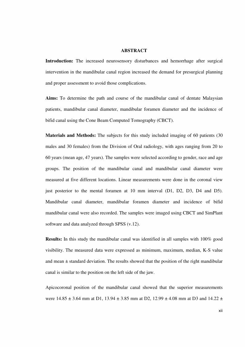
ABSTRACT
Introduction: The increased neurosensory disturbances and hemorrhage after surgical
intervention in the mandibular canal region increased the demand for presurgical planning
and proper assessment to avoid those complications.
Aims: To determine the path and course of the mandibular canal of dentate Malaysian
patients, mandibular canal diameter, mandibular foramen diameter and the incidence of
bifid canal using the Cone Beam Computed Tomography (CBCT).
Materials and Methods: The subjects for this study included imaging of 60 patients (30
males and 30 females) from the Division of Oral radiology, with ages ranging from 20 to
60 years (mean age, 47 years). The samples were selected according to gender, race and age
groups. The position of the mandibular canal and mandibular canal diameter were
measured at five different locations. Linear measurements were done in the coronal view
just posterior to the mental foramen at 10 mm interval (D1, D2, D3, D4 and D5).
Mandibular canal diameter, mandibular foramen diameter and incidence of bifid
mandibular canal were also recorded. The samples were imaged using CBCT and SimPlant
software and data analyzed through SPSS (v.12).
Results: In this study the mandibular canal was identified in all samples with 100% good
visibility. The measured data were expressed as minimum, maximum, median, K-S value
and mean ± standard deviation. The results showed that the position of the right mandibular
canal is similar to the position on the left side of the jaw.
Apicocoronal position of the mandibular canal showed that the superior measurements
were 14.85 ± 3.64 mm at D1, 13.94 ± 3.85 mm at D2, 12.99 ± 4.08 mm at D3 and 14.22 ±
xiii
1.52 mm at D4. The inferior measurements of the canal was 9.37 ± 1.69 mm at D1, 8.24 ±
1.69 mm at D2, 7.96 ± 1.93 mm at D3, 9.65 ± 2.54 at D4 and 15.21 ± 4.18 mm at D5. The
buccolingual position were 3.89 ± 1.00 mm (buccal) and 4.33 ± 1.25 mm (lingual), 5.59 ±
1.20 mm (buccal) and 3.35 ± 1.20 mm (lingual), 6.71 ± 1.34 mm (buccal) and 3.25 ± 1.32
mm (lingual), 5.68 ± 1.63 mm (buccal) and 3.08 ± 1.46 mm (lingual), 4.24 ± 1.59 mm
(buccal) and 2.12 ± 1.40 mm (lingual) at D1,D2,D3,D4 and D5 respectively.
The minimum mandibular canal diameter recorded was 2.00 mm and the maximum was
3.40 mm. In this study the average mean was 2.16 ± 0.30 mm with the least mean diameter
at D2 location (2.01 ± 0.42 mm) and the largest mean diameter at D1 (2.25 ± 0.47 mm) and
D5 (2.25 ± 0.43 mm). The average mandibular formamen diameter was measured to be
2.55 ±0.43 mm.
The incidence of bifid mandibular canal was greatest in Malays (n=18), followed by
Indians (n=9), while no bifid canal was noticed in the Chinese.
Conclusion: Position of the canal changes due to changes in the mandibular bone.
Measurements showed that the mandibular canal curves toward the lingual side the more
distal it is away from the mental foramen. Apicocoronal assessment of the canal reveals
that it is curving downward towards the inferior mandibular border until D3 and then it
curves upwards. This CBCT study reveals there are variations in the position of the
mandibular canal. It is highly recommended that careful assessment and planning using
computed tomographic imaging is done prior to any surgical intervention in the mandibular
canal region to avoid untoward complications.
Keywords: Cone Beam Computed Tomography (CBCT), Mandibular Canal, Inferior
Alveolar Nerve (IAN), Simplant Software, Malaysian Population, Indian, Chinese, Malays
xiv
LIST OF TABLES
Table Description Page
Table 3.1 Selection of cases based on the gender and ethnicity (race) 48
Table 3.2 Age group distribution of samples 49
Table 3.3 Landmarks and base lines record 53
Table 4.1 Comparison of length measurements for all Ds locations on the right and
left sides
60
Table 4.2 Descriptive statistics of D1 length measurements 61
Table 4.3 Comparison of D1 mean measurements by ethnicity (race) 62
Table 4.4 Comparison of D1 mean measurements between males and females 63
Table 4.5 Comparison of D1 mean measurements between gender among Malays 64
Table 4.6 Comparison of D1 mean measurements between gender among Chinese 65
Table 4.7 Comparison of D1 mean measurements between gender among Indians 66
Table 4.8 Comparison of D1 mean measurements between age groups 67
Table 4.9 Descriptive statistics of D2 length measurements 68
Table 4.10 Comparison of D2 mean measurements by ethnicity (race) 69
Table 4.11 Comparison of D2 mean measurements between males and females 70
Table 4.12 Comparison of D2 mean measurements between gender among Malays 71
Table 4.13 Comparison of D2 mean measurements between gender among Chinese 72
Table 4.14 Comparison of D2 mean measurements between gender among Indians 73
Table 4.15 Comparison of D2 mean measurements between age groups 74
Table 4.16 Descriptive statistics of D3 length measurements 75
Table 4.17 Comparison of D3 mean measurements by ethnicity (race) 76
Table 4.18 Comparison of D3 mean measurements between males and females 77
Table 4.19 Comparison of D3 mean measurements between gender among Malays 78
Table 4.20 Comparison of D3 mean measurements between gender among Chinese 79
xv
Table 4.21 Comparison of D3 mean measurements between gender among Indians 80
Table 4.22 Comparison of D3 mean measurements between age groups 81
Table 4.23 Descriptive statistics of D4 length measurements 82
Table 4.24 Comparison of D4 mean measurements by ethnicity (race) 83
Table 4.25 Comparison of D4 mean measurements between males and females 84
Table 4.26 Comparison of D4 mean measurements between gender among Malays 85
Table 4.27 Comparison of D4 mean measurements between gender among Chinese 86
Table 4.28 Comparison of D4 mean measurements between gender among Indians 86
Table 4.29 Comparison of D4 mean measurements between age groups 87
Table 4.30 Descriptive statistics of D5 length measurements 88
Table 4.31 Comparison of D5 mean measurements by ethnicity (race) 89
Table 4.32 Comparison of D5 mean measurements between males and females 90
Table 4.33 Comparison of D5 mean measurements between gender among Malays 91
Table 4.34 Comparison of D5 mean measurements between gender among Chinese 92
Table 4.35 Comparison of D5 mean measurements between gender among Indians 93
Table 4.36 Comparison of D5 mean measurements between age groups 94
Table 4.37 Descriptive statistics of the mandibular canal diameter measurements 95
Table 4.38 Comparison of the MC diameter measurements by ethnicity (race) 96
Table 4.39 Comparison of the MC diameter measurements between gender 96
Table 4.40 Comparison of the MC mean measurements between gender among races 97
Table 4.41 Comparison of the MC diameter measurements between age groups 99
Table 4.42 Descriptive statistics of mandibular foramen diameter measurements 99
Table 4.43 Comparison of mandibular foramen diameter mean measurements by
ethnicity (race)
100
Table 4.44 Comparison of mandibular foramen diameter mean measurements between
males and females
100
Table 4.45 Comparison of the MF diameter mean measurements between gender
among races
101
xvi
Table 4.46 Comparison of mandibular foramen diameter mean measurements between
age groups
102
Table 4.47 Frequency and Percentage of the bifid canal in sample studied 103
Table 4.48 Frequency and Percentage of the bifid canal among races 104
Table 4.49 Comparison of the bifid canal among gender 105
Table 5.1 Comparison of studies locating the mandibular canal vertically 114
Table 5.2 Comparison of studies locating the mandibular canal horizontally 117
Table 5.3 Comparison of the MC diameter among different research studies 124
Table 5.4 Comparison of the bifid mandibular canal occurrence in different studies 126
xvii
LIST OF FIGURES
Figure Description Page
Figure 2.1 A reconstructed panoramic image displayed in a thin section to show
the bilateral course of the mandibular canals
6
Figure 2.2 Variations of the vertical position of the inferior alveolar nerve 9
Figure 2.3 Bifid MC 13
Figure 2.4 Illustrated diagram of the anatomy of trigeminal nerve 14
Figure 2.5 Neurovascular bundle 15
Figure 2.6 Illustrated diagrams for inferior alveolar nerve injury by implant drill 19
Figure 2.7 Illustrated diagrams for inferior alveolar nerve injury by dental implant 21
Figure 2.8 The orthopantomograph shows the disrupted superior border of
mandibular canal and cancellous bone which has few and thin
trabecullae
26
Figure 2.9 Computed tomographic images 34
Figure 2.10 Cone beam computed tomography system showing the x-ray source
and the receptor
38
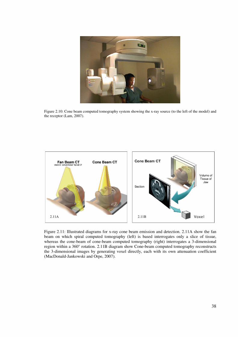
Figure 2.11 Illustrated diagrams for x-ray cone beam emission and detection 38
Figure 2.15 SimPlant Workstation 49
Figure 3.1 Illustrated diagram for the measurements at the coronal view of the
jaw
52
Figure 3.2 Illustrating locations of measurements at every 1cm interval starting
from the distal aspect of mental foramen backwards (D1-D5).
53
Figure 3.3 Flow Chart showing the methodology of the study 55
Figure 4.1 Mandibular canal position at each location considered in this study
(D1-D5) -coronal view of CBCT image improved with SimPlant
software
58
xviii
Figure 4.2 A.Mandibular canal diameter measurements, B.Mandibular foramen
diameter measurements – coronal view of CBCT image improved with
Simplant software.
102
Figure 4.3 Bifid mandibular canal frequencies among gender 103
Figure 4.4 Bifid mandibular canal frequencies among Malays and Indians 104
Figure 4.5 Bifid mandibular canal – panoramic view of CBCT image improved
with Simplant software
105
Figure 5.1 Illustrated diagram of the mandibular canal path – axial view 118
Figure 5.2 Illustrated diagram of the mandibular canal path – coronal view 118
Figure 5.3 Illustrated diagram of the mandibular canal path among race – axial
view
119
Figure 5.4 Illustrated diagram of the mandibular canal path among race – coronal
view
120
Figure 5.5 Illustrated diagram of the mandibular canal path among age groups –
axial view
122
Figure 5.6 Illustrated diagram of the mandibular canal path among age groups –
coronal view
123
Figure 7.1 Illustrated diagram showing positions included in the application 131
Figure 7.2 Screenshot from the developed software 132

xix
LIST OF SYMBOLS AND ABBREVIATIONS
IAN Inferior alveolar nerve
CBCT Cone Beam Computed Tomography
MC Mandibular canal
MF Mandibular foramen
B Buccal
L Lingual
I Inferior
S Superior
BSSO Bilateral sagital split osteotomy
CT Computed Tomography
MPR Multiplanar Reconstruction
D1 The location of the mandibular canal at the distal aspect of mental foramen
D2 The location of the mandibular canal at 10 mm away from D1 distally
D3 The location of the mandibular canal at 10 mm away from D2 distally
D4 The location of the mandibular canal at 10 mm away from D3 distally
D5 The location of the mandibular canal at 10 mm away from D4 distally
MCd The mandibular canal diameter measurements
ManFd The mandibular foramen diameter measurements
2D Two dimensional
3D Three dimensional
SCT spiral computerized tomography
HR-CT High resolution computed tomography
HR-MRI High resolution magnetic resonance imaging
IMB Inferior mandibular border
LC Virtual horizontal line touching the highest buccal point of the alveolar crest
1
CHAPTER 1
INTRODUCTION
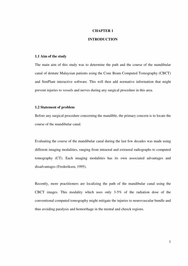
1.1 Aim of the study
The main aim of this study was to determine the path and the course of the mandibular
canal of dentate Malaysian patients using the Cone Beam Computed Tomography (CBCT)
and SimPlant interactive software. This will then add normative information that might
prevent injuries to vessels and nerves during any surgical procedure in this area.
1.2 Statement of problem
Before any surgical procedure concerning the mandible, the primary concern is to locate the
course of the mandibular canal.
Evaluating the course of the mandibular canal during the last few decades was made using
different imaging modalities, ranging from intraoral and extraoral radiographs to computed
tomography (CT). Each imaging modalities has its own associated advantages and
disadvantages (Frederiksen, 1995).
Recently, more practitioners are localizing the path of the mandibular canal using the
CBCT images. This modality which uses only 3-5% of the radiation dose of the
conventional computed tomography might mitigate the injuries to neurovascular bundle and
thus avoiding paralysis and hemorrhage in the mental and cheeck regions.
2
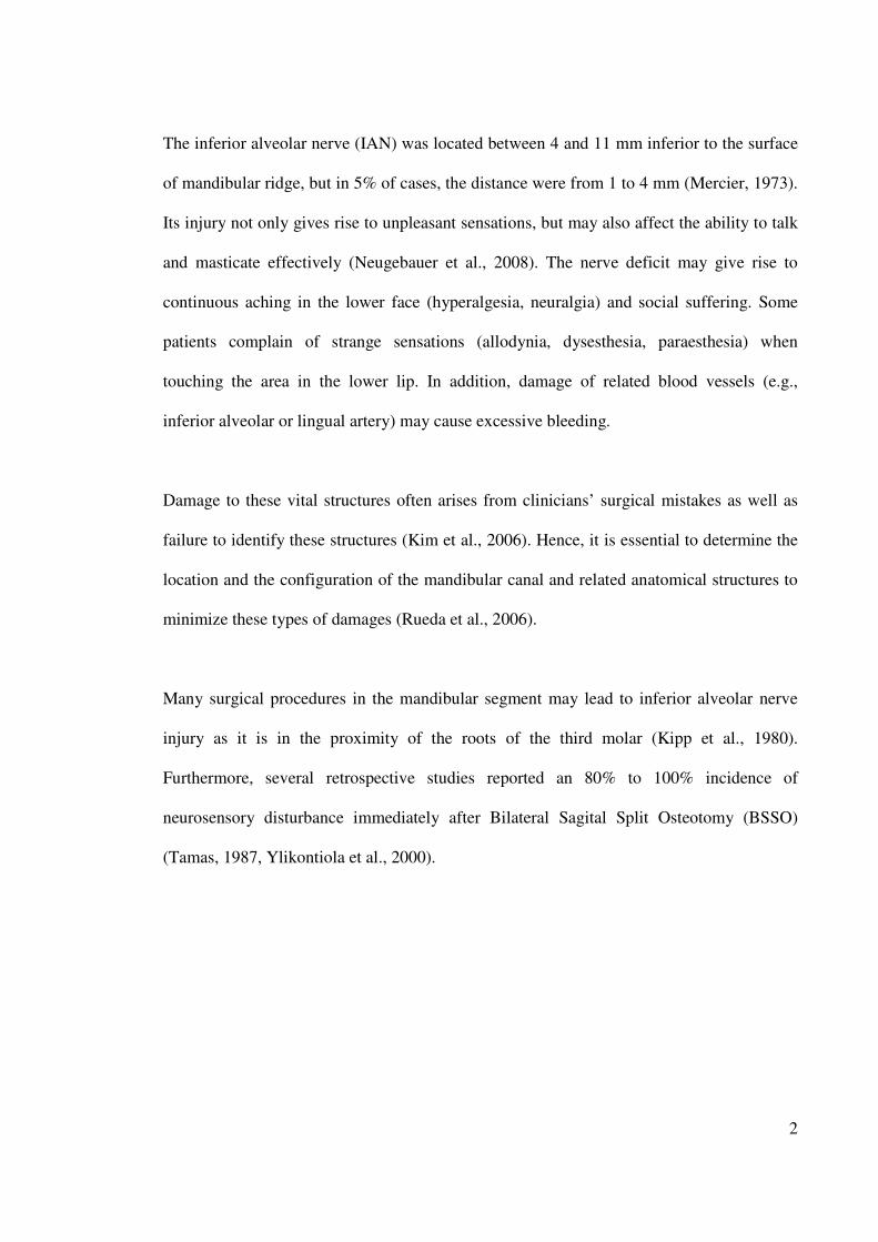
The inferior alveolar nerve (IAN) was located between 4 and 11 mm inferior to the surface
of mandibular ridge, but in 5% of cases, the distance were from 1 to 4 mm (Mercier, 1973).
Its injury not only gives rise to unpleasant sensations, but may also affect the ability to talk
and masticate effectively (Neugebauer et al., 2008). The nerve deficit may give rise to
continuous aching in the lower face (hyperalgesia, neuralgia) and social suffering. Some
patients complain of strange sensations (allodynia, dysesthesia, paraesthesia) when
touching the area in the lower lip. In addition, damage of related blood vessels (e.g.,
inferior alveolar or lingual artery) may cause excessive bleeding.
Damage to these vital structures often arises from clinicians’ surgical mistakes as well as
failure to identify these structures (Kim et al., 2006). Hence, it is essential to determine the
location and the configuration of the mandibular canal and related anatomical structures to
minimize these types of damages (Rueda et al., 2006).
Many surgical procedures in the mandibular segment may lead to inferior alveolar nerve
injury as it is in the proximity of the roots of the third molar (Kipp et al., 1980).
Furthermore, several retrospective studies reported an 80% to 100% incidence of
neurosensory disturbance immediately after Bilateral Sagital Split Osteotomy (BSSO)
(Tamas, 1987, Ylikontiola et al., 2000).
3
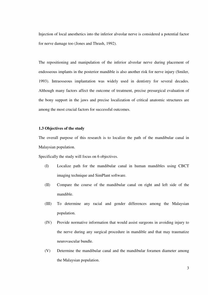
Injection of local anesthetics into the inferior alveolar nerve is considered a potential factor
for nerve damage too (Jones and Thrash, 1992).
The repositioning and manipulation of the inferior alveolar nerve during placement of
endosseous implants in the posterior mandible is also another risk for nerve injury (Smiler,
1993). Intraosseous implantation was widely used in dentistry for several decades.
Although many factors affect the outcome of treatment, precise presurgical evaluation of
the bony support in the jaws and precise localization of critical anatomic structures are
among the most crucial factors for successful outcomes.
1.3 Objectives of the study
The overall purpose of this research is to localize the path of the mandibular canal in
Malaysian population.
Specifically the study will focus on 6 objectives.
(I) Localize path for the mandibular canal in human mandibles using CBCT
imaging technique and SimPlant software.
(II) Compare the course of the mandibular canal on right and left side of the
mandible.
(III) To determine any racial and gender differences among the Malaysian
population.
(IV) Provide normative information that would assist surgeons in avoiding injury to
the nerve during any surgical procedure in mandible and that may traumatize
neurovascular bundle.
(V) Determine the mandibular canal and the mandibular foramen diameter among
the Malaysian population.
4
(VI) Indicate the frequency of the bifid mandibular canal using CBCT imaging
technique and SimPlant software among the Malaysian population.
1.4 Research Questions
Based upon the objectives mentioned previously, this research study aims to answer the
following questions:
(I) What is the path for the mandibular canal in human mandibles among the
Malaysian population?
(II) Is there any difference between the right and the left mandibular canal metrical
measurements?
(III) Is there any difference between the races and gender among the Malaysian
population?
(IV) What is the information gained from this research that will help surgeons and
practitioners to minimize any injury to the mandibular canal during any surgical
intervention in the mandible?
(V) What is the diameter for the mandibular canal and the mandibular foramen
among the Malaysian population?
(VI) What is the frequency of bifid mandibular canal among the Malaysian
population?
5
1.5 Significance of the study
This study is the first local study to be carried out on three major races of the Malaysian
population. These results may be used as a safety guide during surgical procedures in oral
implantology cases and oral and maxillofacial surgery to prevent postoperative
complications. This is a landmark study done on life patients with CBCT and 3D
simulation which must be very accurate.
Studies on the comparison between right and left mandibular canal measurements were
made and this shall provide a guide as to whether future researchers shall include both or
one side of the mandible for their research among the Malaysian population.
1.6 Choice of the study topic
There are four main reasons behind choosing the topic of this study which are, Firstly, no
such studies had previously been done in a Malaysian population Secondly, the number of
practitioners performing implant surgery has increased dramatically over the last fifteen
years. Thirdly, studies showed that IAN is the most commonly injured nerve in the
mandible. Lastly, the use of CBCT as the imaging technique was chosen as it is non-
invasive and emits low radiation onto the patient.
6
CHAPTER 2
REVIEW OF RELATED LITERATURE
2.1 Anatomical Consideration
The mandibular canal is a canal within the mandible that houses the inferior alveolar nerve
(a.k.a. mandibular nerve), the inferior alveolar artery and the inferior alveolar vein
(Tammisalo et al., 1992). The canal is seen bilaterally as it enters the mandible at the
mandibular foramen on the lingual side of the ramus. It runs obliquely downward and
forward in the ramus, and then horizontally forward in the body, where it is placed under
the alveloi and communicates with them by small openings (Williams et al., 1989). On
arriving at the incisor teeth, it turns back to communicate with the mental foramen, giving
off two small canals which run to the cavities containing the incisor teeth (Greenstein and
Tarnow, 2006).
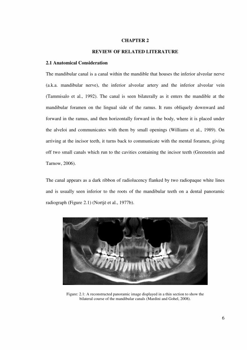
The canal appears as a dark ribbon of radiolucency flanked by two radiopaque white lines
and is usually seen inferior to the roots of the mandibular teeth on a dental panoramic
radiograph (Figure 2.1) (Nortjĕ et al., 1977b).
Figure: 2.1: A reconstructed panoramic image displayed in a thin section to show the
bilateral course of the mandibular canals (Mardini and Gohel, 2008).
7
The study of Rajchel et al. (1986) employing panoramic radiograph of 45 Asian adults
demonstrated that the mandibular canal, when proximal to the third molar region, is usually
a single large structure, 2.0 to 2.4 mm in diameter. While Obradovic et al. (1993) measured
105 cadaveric mandibles and found the average diameter of the mandibular canal in its
horizontal part is 2.6 mm. Ikeda et al. (1996) conducted similar cadaver study and reported
that the canal is approximately 3.4 mm wide.
2.2 Anatomical Variations
Different anatomical variations in the course of the mandibular canal (superior-inferior and
bucco-lingual) were described in many studies. Bifid canal was noticed in many research
studies (Sanchis et al., 2003).
2.2.1 Vertical position
Root apices of mandibular teeth and the inferior border of the mandible were considered as
anatomical landmarks to evaluate and determine the vertical position of the mandibular
canal in many studies. Thus, Heasman (1988) reported that from a study of 96 plain films
of dried mandibles, in 68% of cases the mandibular canal passed along an intermediate
course between the mandibular root apices and the inferior border of the mandible. Rajchel
et al. (1986) reported that proximal to the third molar a mean distance of 10 mm was
noticed between the mandibular canal and the inferior mandibular border. It has also been
shown that the upper border of the mandibular canal was located 3.5 to 5.4 mm below the
root apices of the first and second molars (Littner et al., 1986). Denio et al. (1992)
conducted their research on 22 cadavers and found the mean distance of the mandibular
canal to the apices of mandibular second molar, the first molar and second premolar were
3.7, 6.9, and 4.7 mm respectively.
8
Sato et al. (2005) defined the presence and course of the mandibular canal using
macroscopic cadaveric dissection, CT and panoramic X-ray observation. Panoramic X-ray
observation revealed that the vertical position of the mandibular canal was closer to the
apices of the first and the second molars than that to the distance of inferior border of
mandible. The mandibular canal position was measured within 30% of the ratio from the
distance of inferior border of mandible to the apices of the roots (mesial root of the first
molar: 20%; distal root of the first molar: 22.6%; mesial root of the second molar: 27.8%
and distal root of the second molar: 47%) on panoramic X-ray observation. All classic
descriptions of the mandibular canal course mentioned above refer to dentate mandibles.
Greenstein et al. (2008) revealed that the mandibular canal is fairly close to the apices of
the second molar in 50% of the radiographs. In 40%, the canal is away from the root apices,
and in only 10% of the radiographs the root apices appeared to penetrate the canal.
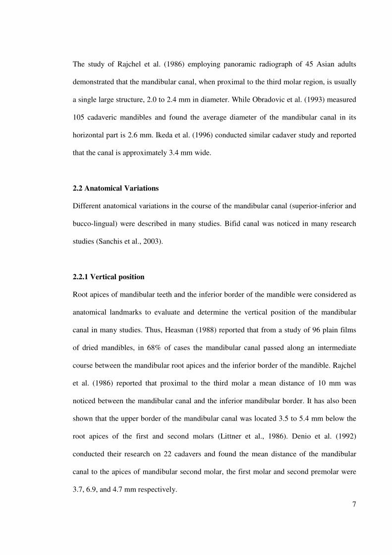
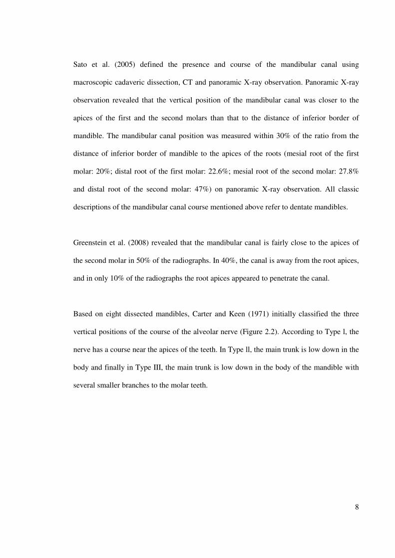
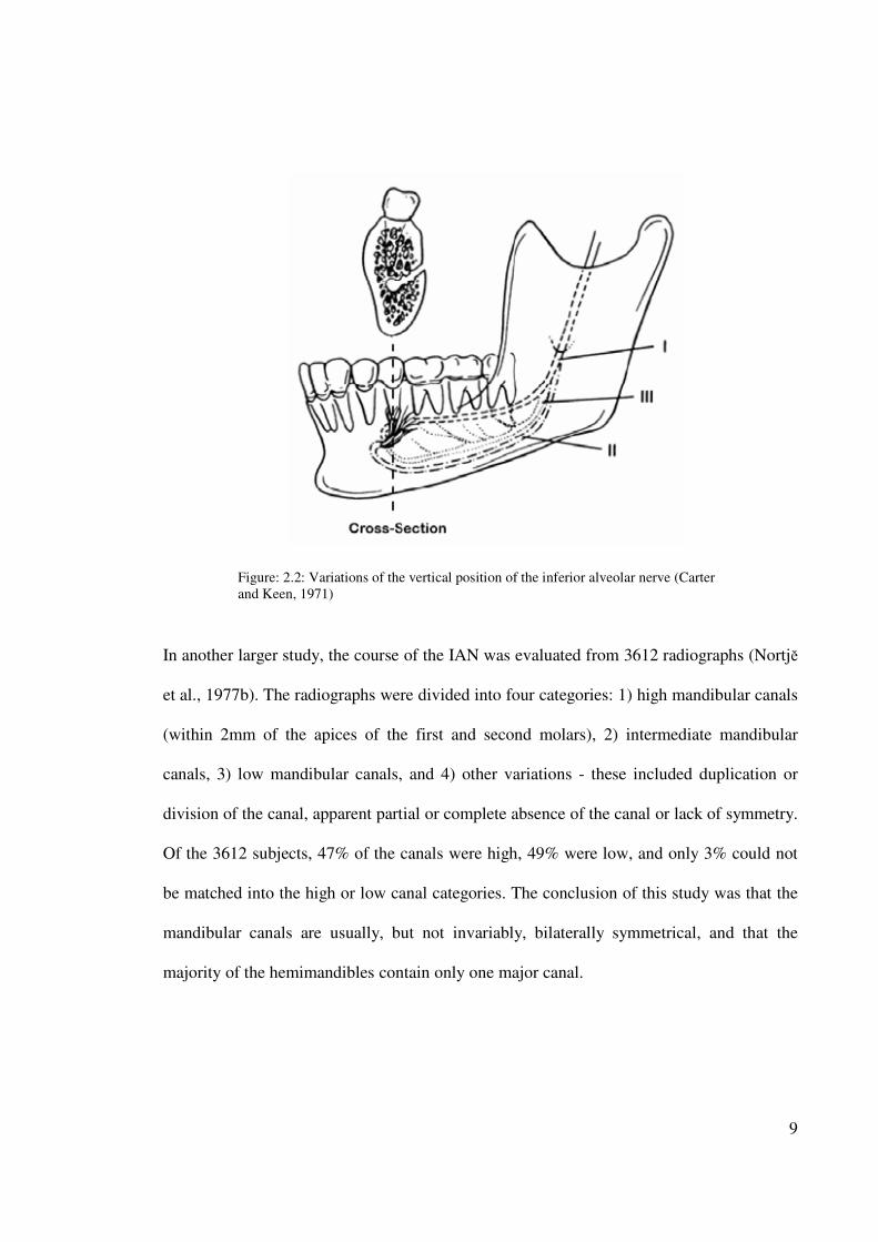
Based on eight dissected mandibles, Carter and Keen (1971) initially classified the three
vertical positions of the course of the alveolar nerve (Figure 2.2). According to Type l, the
nerve has a course near the apices of the teeth. In Type ll, the main trunk is low down in the
body and finally in Type III, the main trunk is low down in the body of the mandible with
several smaller branches to the molar teeth.
9
Figure: 2.2: Variations of the vertical position of the inferior alveolar nerve (Carter
and Keen, 1971)
In another larger study, the course of the IAN was evaluated from 3612 radiographs (Nortjĕ
et al., 1977b). The radiographs were divided into four categories: 1) high mandibular canals
(within 2mm of the apices of the first and second molars), 2) intermediate mandibular
canals, 3) low mandibular canals, and 4) other variations - these included duplication or
division of the canal, apparent partial or complete absence of the canal or lack of symmetry.
Of the 3612 subjects, 47% of the canals were high, 49% were low, and only 3% could not
be matched into the high or low canal categories. The conclusion of this study was that the
mandibular canals are usually, but not invariably, bilaterally symmetrical, and that the
majority of the hemimandibles contain only one major canal.
10
Anderson et al.(1991) reported that the buccal-lingual and superior-inferior positions of the
inferior alveolar nerve were not consistent among mandibles. The inferior alveolar nerve
frequently showed as concave curve when descending at the posterior segment and then
progressed anteriorly. At the anterior segment the nerve ascended to the mental foramen.
He further stated that a bony canal was not always visible and the canal itself frequently
lacked definite walls, especially in the vicinity of the mental foramen. Bilateral symmetry
was commonly observed, while on the other hand duplications of the canal were rare.
Kieser et al.(2004) also studied vertical positioning and intra-bony branching patterns of the
inferior alveolar nerve in 39 edentulous mandibles. This was possible as the researchers
undertook micro-dissections. Classification is done according to height of the inferior
alveolar nerve within the body of the mandible and the branching pattern of the inferior
alveolar nerve. In 30.7% (12/39) of the cases, the IAN was located in the superior part of
the body of the mandible, and in 69.3% (27/39) of the cases the IAN was half-way or closer
to the inferior border of the mandible.
In another study with 107 edentulous human cadaveric mandibles by Kieser et al.(2005),
found that for 73% of males and 70% of females the IAN was located in the lower half of
the mandible. The most common branching pattern observed was a single nerve trunk with
a series of simple branches directed at the superior border of the mandible (59.6% males,
52% females). The second most common pattern was that of a small nerve plexus in the
molar region (21.1% males, 26% females). This study showed that the pattern of
distribution does not significantly differ between the sexes, between sides of the jaw, or
with age.
11
Narayana and Vasudha (2004) evaluated the position of the mandibular foramen and the
course of the IAN. This study concluded that the canal and consequently the nerve do not
maintain a constant position in the mandible and the location of the mandibular foramen
varies despite its bilateral symmetry.
Mandibular alveolar bone undergoes resorption in a varying degree when the mandibular
teeth are lost (Lavelle, 1985, Polland et al., 2001). The dental ridge becomes lower during
mandible atrophy, and this is why Levine et al. (2007) measured the distance from the
edentulous alveolar crest to the superior aspect of the MC of 50 patients who had a
radiographically identifiable mandibular canal and at least one mandibular first molar.
Results showed that the superior aspect of the MC was 17.4 mm inferior from the alveolar
crest. Similarly, Watanabe et al. (2009) analyzed CT data of 79 Japanese patients (52 males
and 27 females) and found that the distance from the alveolar crest to the mandibular canal
ranged from 15.3 to 17.4 mm. It is clear that the distance between the mandibular canal and
the atrophic alveolar ridge is a variable dimension and should be assessed in each particular
case.
2.2.2 Horizontal position
It was reported that the mandibular canal might have different anatomic configurations in
the horizontal plane. Usually the mandibular canal crosses from the lingual to the buccal
side of the mandible and in most cases the midway between the buccal and lingual cortical
plates of bone is at the first molar (Miller et al., 1990, Obradovic et al., 1995). According to
Rajchel et al.(1986), the mandibular canal, when proximal to the third molar region,
courses approximately 2.0 mm from the inner lingual cortex, 1.6 to 2.0 mm from the medial
aspect of the buccal plate.
12
Levine et al.(2007) assessed the mandibular canal buccolingual course for 50 patients. The
mean buccal aspect of the canal was 4.9 mm from the buccal cortical margin of the
mandible. They found that age and race were statistically associated with the mandibular
canal position. Older patients and white patients have less distance between the buccal
aspect of the canal and the buccal mandibular border.
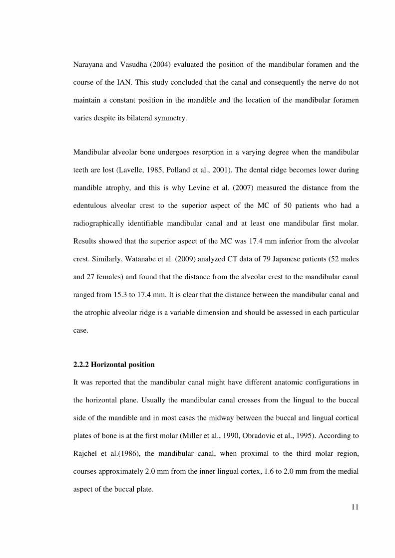
2.3 Bifid mandibular canal (MC)
Bifid variety of the mandibular canals which are characterized by a single mandibular
foramen and two nearly equal canals are indeed unusual (Figure 2.3). In the study
employing panoramic radiographs, Nortjĕ et al. (1977b), reported that duplication or
division of the canal was found in 0.90% (33/3612) of the cases. In another study by Grover
and Lorton (1983) showed that 0.08% bifurcation of the inferior alveolar nerve canal was
found in 5000 US Army soldiers, aged 17 to 26 years. Furthermore, Langlais et al. (1985),
evaluated routine panoramic radiographs of 6000 patients, they found 57 (0.95%) cases of
bifid inferior mandibular canals, 19 in males and 38 in females. Another study on 2012
panoramic radiographs reported that 0.35% of canals were bifid and all cases were
registered in women (Sanchis et al., 2003). Utilizing CBCT technology (Naitoh et al.,
2009a) reconstructed 122 2D images of various planes in the mandibular ramus region to
the computer program using 3D visualization and measurement software. Bifid mandibular
canal in the mandibular ramus region was observed in 65% of patients and 43% of sides.
Furthermore, they classified bifid mandibular canal into four types: retromolar, dental,
forward, and buccolingual canals.
13
Figure 2.3: Bifid MC (Claeys and Wackens, 2005)
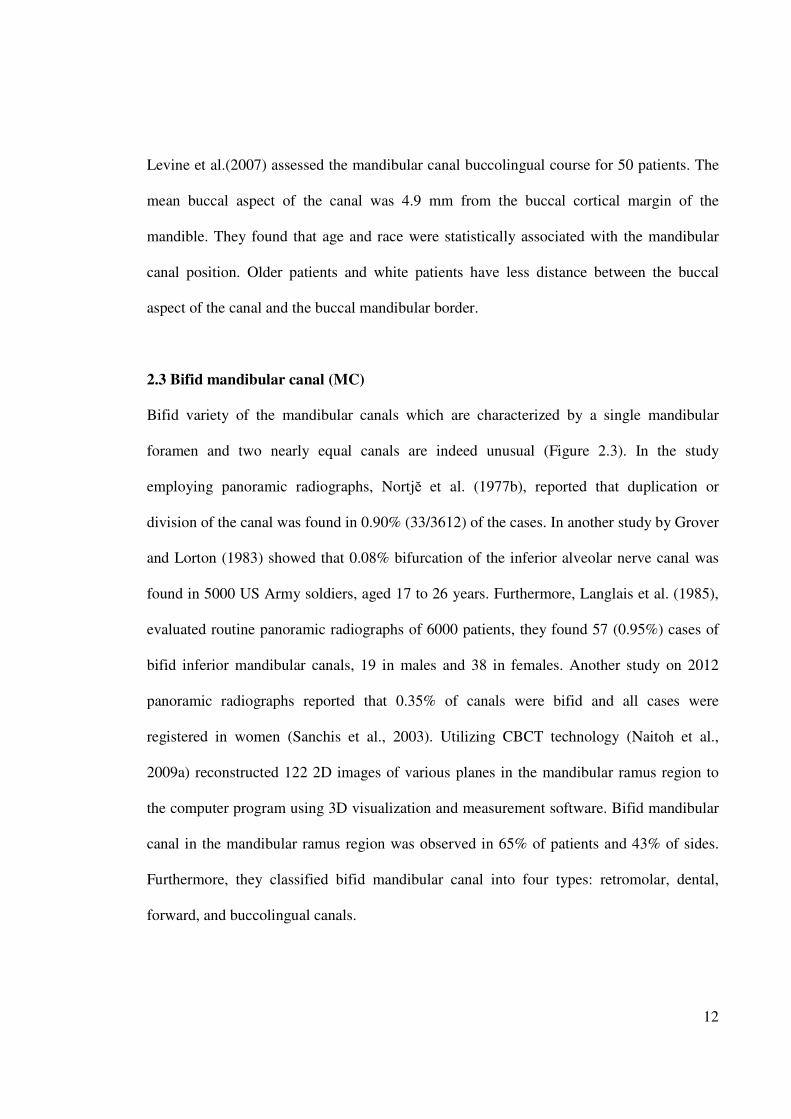
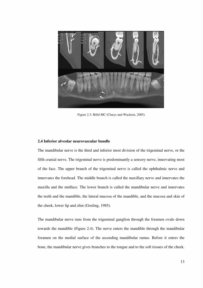
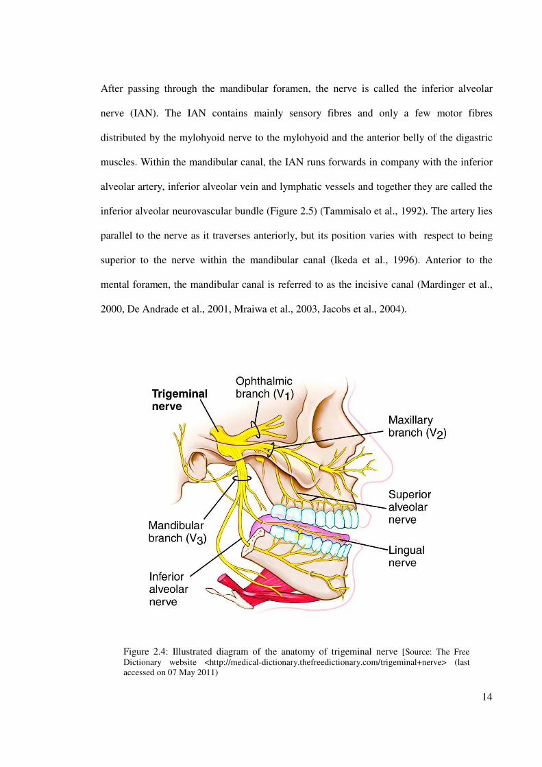
2.4 Inferior alveolar neurovascular bundle
The mandibular nerve is the third and inferior most division of the trigeminal nerve, or the
fifth cranial nerve. The trigeminal nerve is predominantly a sensory nerve, innervating most
of the face. The upper branch of the trigeminal nerve is called the ophthalmic nerve and
innervates the forehead. The middle branch is called the maxillary nerve and innervates the
maxilla and the midface. The lower branch is called the mandibular nerve and innervates
the teeth and the mandible, the lateral mucosa of the mandible, and the mucosa and skin of
the cheek, lower lip and chin (Gosling, 1985).
The mandibular nerve runs from the trigeminal ganglion through the foramen ovale down
towards the mandible (Figure 2.4). The nerve enters the mandible through the mandibular
foramen on the medial surface of the ascending mandibular ramus. Before it enters the
bone, the mandibular nerve gives branches to the tongue and to the soft tissues of the cheek.
14
After passing through the mandibular foramen, the nerve is called the inferior alveolar
nerve (IAN). The IAN contains mainly sensory fibres and only a few motor fibres
distributed by the mylohyoid nerve to the mylohyoid and the anterior belly of the digastric
muscles. Within the mandibular canal, the IAN runs forwards in company with the inferior
alveolar artery, inferior alveolar vein and lymphatic vessels and together they are called the
inferior alveolar neurovascular bundle (Figure 2.5) (Tammisalo et al., 1992). The artery lies
parallel to the nerve as it traverses anteriorly, but its position varies with respect to being
superior to the nerve within the mandibular canal (Ikeda et al., 1996). Anterior to the
mental foramen, the mandibular canal is referred to as the incisive canal (Mardinger et al.,
2000, De Andrade et al., 2001, Mraiwa et al., 2003, Jacobs et al., 2004).
Figure 2.4: Illustrated diagram of the anatomy of trigeminal nerve [Source: The Free
Dictionary website <http://medical-dictionary.thefreedictionary.com/trigeminal+nerve> (last
accessed on 07 May 2011)
15
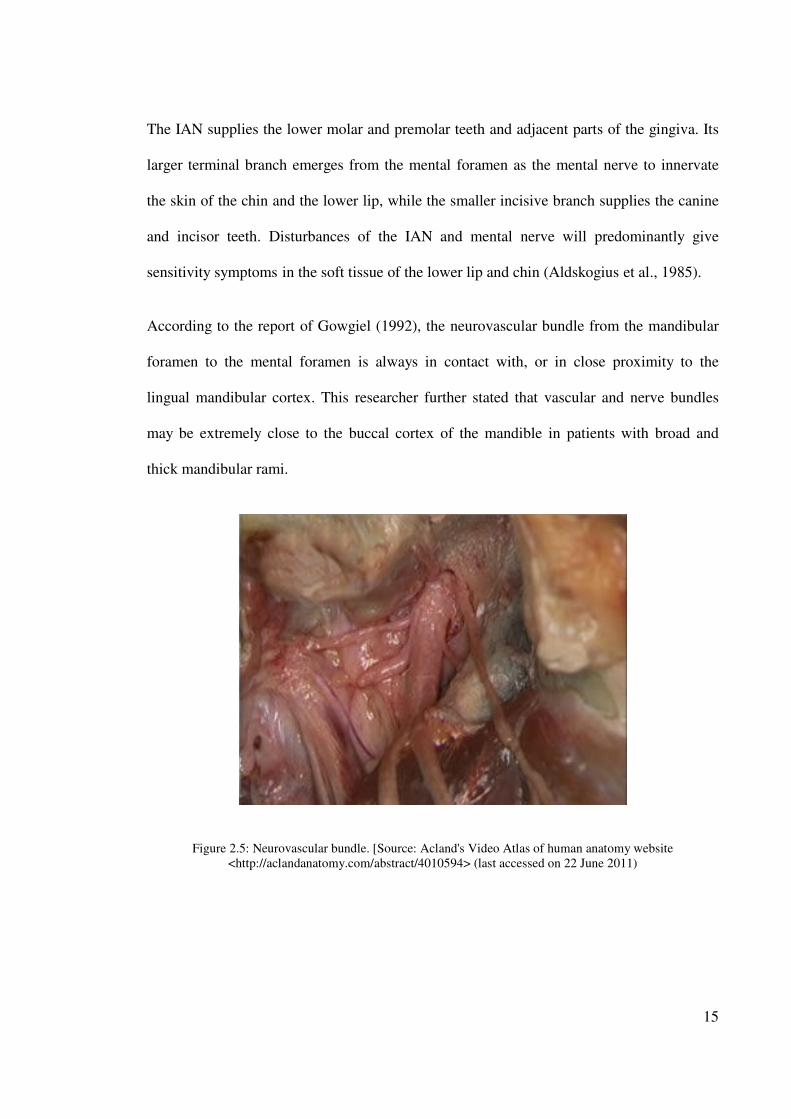
The IAN supplies the lower molar and premolar teeth and adjacent parts of the gingiva. Its
larger terminal branch emerges from the mental foramen as the mental nerve to innervate
the skin of the chin and the lower lip, while the smaller incisive branch supplies the canine
and incisor teeth. Disturbances of the IAN and mental nerve will predominantly give
sensitivity symptoms in the soft tissue of the lower lip and chin (Aldskogius et al., 1985).
According to the report of Gowgiel (1992), the neurovascular bundle from the mandibular
foramen to the mental foramen is always in contact with, or in close proximity to the
lingual mandibular cortex. This researcher further stated that vascular and nerve bundles
may be extremely close to the buccal cortex of the mandible in patients with broad and
thick mandibular rami.
Figure 2.5: Neurovascular bundle. [Source: Acland's Video Atlas of human anatomy website
<http://aclandanatomy.com/abstract/4010594> (last accessed on 22 June 2011)
16
2.5 Injury of the inferior alveolar nerve
IAN is the most commonly injured nerve in the mandible (64.4%), followed by the lingual
nerve (28.8%) (Tay and Zuniga, 2007). The differences between IAN injuries and other
peripheral sensory nerve injuries are predominantly iatrogenic and not resolved within the
first 2 months after injury (Haskell et al., 1986, Venta et al., 1998). The closed injuries can
also occur that often delays diagnosis and treatment (Pogrel and Maghen, 2001).
The number of practitioners performing implant surgery has increased dramatically over
the last fifteen years. As confidence is gained they tend to accept increasingly challenging
cases and it is to be expected that the incidence of problems and complications will increase
(Worthington, 1995). It was a discerning remark, however, it remains a serious
complication and many had reported the incidences varies from 0 to 40% of implant related
inferior alveolar nerve (IAN) injuries (Wismeijer et al., 1997, Dao and Mellor, 1998,
Bartling et al., 1999). The damage can result from the traumatic local anesthetic injections
or during the dental implant site osteotomy or placement (Kraut and Chahal, 2002). This
damage is one of the most unpleasant experiences for both the patient and the dentist
(Alhassani and AlGhamdi, 2010). As a result, many functions such as speech, eating,
kissing, make-up application, shaving and drinking will be affected (Ziccardi and Assael,
2001).
17
2.5.1 Inferior alveolar nerve (IAN) injury due to implant surgery
Damage of inferior alveolar nerve during dental implant placement can be a serious
complication. Clinician should recognize and exclude aetiological factors leading to nerve
injury. Proper presurgery planning, timely diagnosis and treatment are the key to avoid
nerve sensory disturbances management. There are four possible aetiological factors of
IAN injury during the implant placement and can be summarized as:
2.5.1.1 Inferior alveolar nerve injury during traumatic local anaesthesia injection
Profound local anaesthesia during the dental implant surgery can drastically reduce patient
anxiety during the surgery. Local anaesthetics are designed to prevent sensory impulses
being transmitted from intraoral and extraoral areas to the central nervous system with
minimal effect on muscular tone (Hillerup and Jensen, 2006). Unfortunately, the injury of
an IAN can occur during a traumatic local anaesthesia injection (Malamed, 2010, Jones and
Thrash, 1992).
Three main theories were proposed for the inferior alveolar nerve injury during traumatic
local anaesthesia injection and these includes direct trauma from the injection needle
(Crean and Powis, 1999, Stacy and Hajjar, 1994), hematoma formation (Harn and Durham,
1990, Haas and Lennon, 1995) and neurotoxicity of the local anaesthetic (Pogrel and
Kaban, 1993, Nickel, 1990).
18
2.5.1.2 Inferior alveolar nerve injury by implant drill
The most severe types of injuries are caused by implant drills and implants themselves
(Worthington, 2004). Sensory IAN injuries made by implant drills may be caused by direct
intraoperative (mechanical and chemical) and indirect postoperative trauma (ischemia and
thermal stimuli) (Nazarian et al., 2003). Many implant drills are slightly longer, for drilling
efficiency, than their corresponding implants. Implant drill length varies and must be
understood by the surgeon because the specified length may not reflect an additional
millimetre so called “y” dimension (Alhassani and AlGhamdi, 2010). Lack of knowledge
about this may cause complications (Kraut and Chahal, 2002). Damage to the IAN can
occur when the twist drill or implant encroaches, transects, or lacerates the nerve (Figures
2.6 A and B).
One of the possible intraoperative complications is direct chemical trauma - alkalinic nerve
injuries from irrigation of the implant bed during preparation with sodium hypochlorite.
This solution has not been recommended in practice and should be avoided (Khawaja and
Renton, 2009).
Some sensory IAN injuries evoked by partial perforation of the mandibular canal during the
drilling is caused by indirect postoperative trauma – secondary ischemia of the IAN by
haemorrhage into the canal and scaring process, rather than direct mechanical trauma by the
drill or implant itself (Figure 2.6 C) (Khawaja and Renton, 2009, Lamas Pelayo et al.,
2008).
19
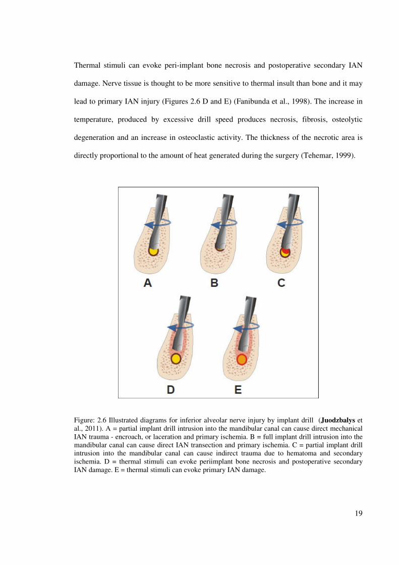
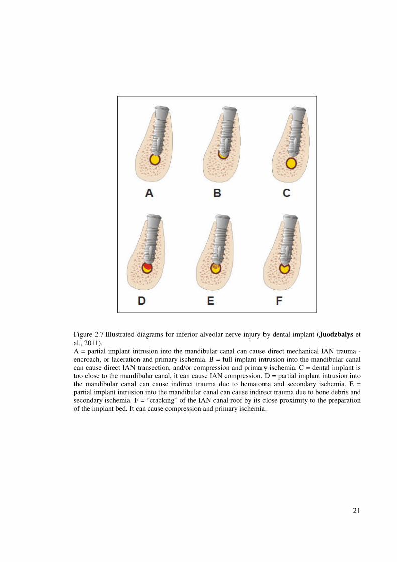
Thermal stimuli can evoke peri-implant bone necrosis and postoperative secondary IAN
damage. Nerve tissue is thought to be more sensitive to thermal insult than bone and it may
lead to primary IAN injury (Figures 2.6 D and E) (Fanibunda et al., 1998). The increase in
temperature, produced by excessive drill speed produces necrosis, fibrosis, osteolytic
degeneration and an increase in osteoclastic activity. The thickness of the necrotic area is
directly proportional to the amount of heat generated during the surgery (Tehemar, 1999).
Figure: 2.6 Illustrated diagrams for inferior alveolar nerve injury by implant drill (Juodzbalys et
al., 2011). A = partial implant drill intrusion into the mandibular canal can cause direct mechanical
IAN trauma - encroach, or laceration and primary ischemia. B = full implant drill intrusion into the
mandibular canal can cause direct IAN transection and primary ischemia. C = partial implant drill
intrusion into the mandibular canal can cause indirect trauma due to hematoma and secondary
ischemia. D = thermal stimuli can evoke periimplant bone necrosis and postoperative secondary
IAN damage. E = thermal stimuli can evoke primary IAN damage.
20
2.5.1.3 Inferior alveolar nerve injury by dental implant
Sensory IAN injuries made by dental implant may be caused by direct intraoperative
(mechanical) and indirect postoperative trauma (ischemia) or periimplant infection
(Nazarian et al., 2003). Direct mechanical injury i.e. encroach, transection, or laceration of
the nerve is related to implant intrusion into the MC (Figures 2.7 A and B).
After a direct trauma that is when the implant is placed through the bony canal, the nerve
ending may get retrograde degeneration in some of the cases, because the nerve running in
the canal is a terminal ending of the nerve and the size is quite small (Beirowski et al.,
2005). Whereas partial implant intrusion into MC can evoke IAN injury due to
compression and secondary ischemia of corresponding neurovascular bundle (Leckel et al.,
2009, Worthington, 2004). This is especially when immediate implantation following tooth
extraction can sometimes cause implant intrusion into MC. Furthermore, efforts by the
surgeon to achieve primary stability can also lead to unintentional apical extension and
subsequent nerve injury. Re-measurement of the amount of available bone after tooth
extraction is recommended especially in those cases of nerve proximity since a few
millimetres of the crestal bone might be lost during the extraction (Alhassani and
AlGhamdi, 2010).
Another cause of injury to the IAN is the displacement of an implant into canal. For
example this is possible in the posterior mandible as the cancellous bone is more abundant
with larger intratrabecular spaces than the anterior mandible (Theisen et al., 1990, Fanuscu
and Chang, 2004).
21
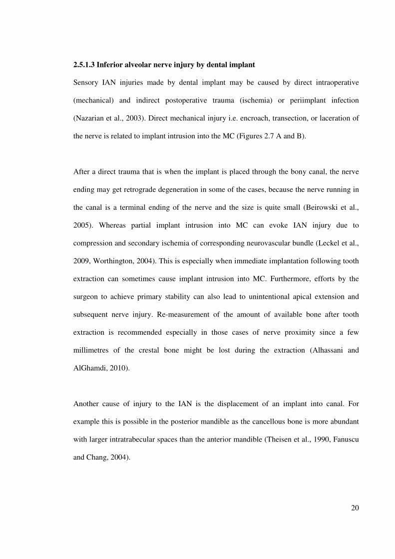
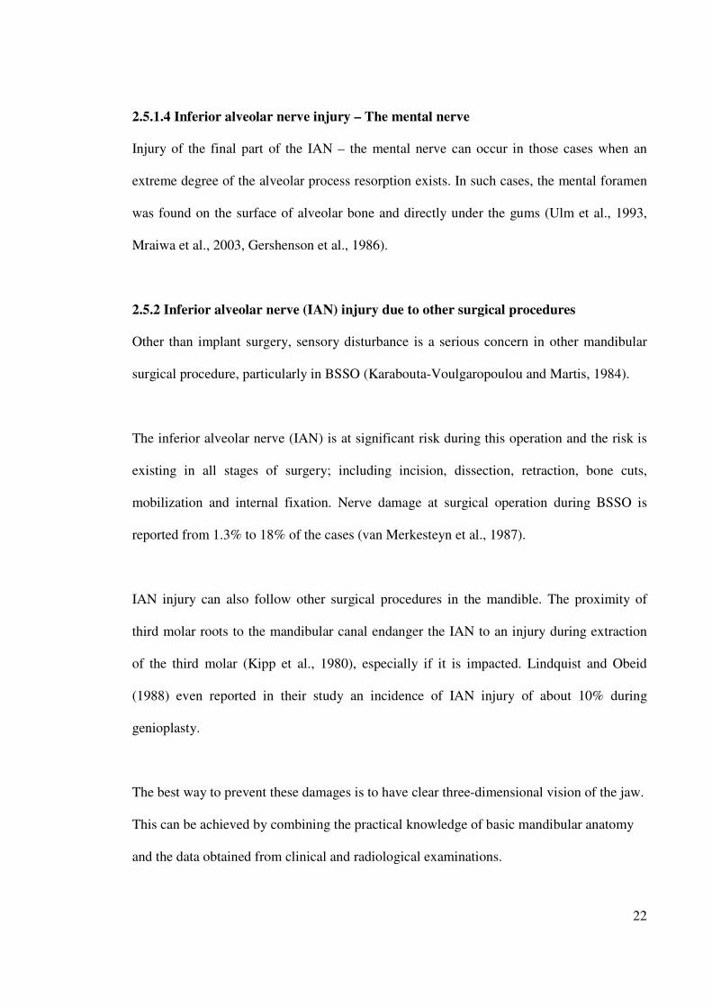
Figure 2.7 Illustrated diagrams for inferior alveolar nerve injury by dental implant (Juodzbalys et
al., 2011).
A = partial implant intrusion into the mandibular canal can cause direct mechanical IAN trauma -
encroach, or laceration and primary ischemia. B = full implant intrusion into the mandibular canal
can cause direct IAN transection, and/or compression and primary ischemia. C = dental implant is
too close to the mandibular canal, it can cause IAN compression. D = partial implant intrusion into
the mandibular canal can cause indirect trauma due to hematoma and secondary ischemia. E =
partial implant intrusion into the mandibular canal can cause indirect trauma due to bone debris and
secondary ischemia. F = “cracking” of the IAN canal roof by its close proximity to the preparation
of the implant bed. It can cause compression and primary ischemia.
22
2.5.1.4 Inferior alveolar nerve injury – The mental nerve
Injury of the final part of the IAN – the mental nerve can occur in those cases when an
extreme degree of the alveolar process resorption exists. In such cases, the mental foramen
was found on the surface of alveolar bone and directly under the gums (Ulm et al., 1993,
Mraiwa et al., 2003, Gershenson et al., 1986).
2.5.2 Inferior alveolar nerve (IAN) injury due to other surgical procedures
Other than implant surgery, sensory disturbance is a serious concern in other mandibular
surgical procedure, particularly in BSSO (Karabouta-Voulgaropoulou and Martis, 1984).
The inferior alveolar nerve (IAN) is at significant risk during this operation and the risk is
existing in all stages of surgery; including incision, dissection, retraction, bone cuts,
mobilization and internal fixation. Nerve damage at surgical operation during BSSO is
reported from 1.3% to 18% of the cases (van Merkesteyn et al., 1987).
IAN injury can also follow other surgical procedures in the mandible. The proximity of
third molar roots to the mandibular canal endanger the IAN to an injury during extraction
of the third molar (Kipp et al., 1980), especially if it is impacted. Lindquist and Obeid
(1988) even reported in their study an incidence of IAN injury of about 10% during
genioplasty.
The best way to prevent these damages is to have clear three-dimensional vision of the jaw.
This can be achieved by combining the practical knowledge of basic mandibular anatomy
and the data obtained from clinical and radiological examinations.
23
2.6 Radiographic methods used to locate the mandibular canal
The location and configuration of the mandibular canal is important in imaging diagnosis
for most surgical procedure of the mandible. Therefore special attention should be given to
the exact location of the mandibular canal, thereby avoiding the neurovascular bundle.
Periapical radiographs were used for many years to assess the jaws pre- and post-implant
placement (van der Stelt, 2005). Similarly panoramic projection were used for diagnostic
purposes where the canal is identifiable as a narrow radiolucent ribbon bordered by
radioopaque lines (Nortjĕ et al., 1977a), but the buccolingual location of the mandibular
canal cannot be obtained on this image.
To obtain the more precise location of the mandibular canal, the clinician may use different
tomography modalities. Tomography can be utilized to section or slice an object. This is
accomplished by the simultaneous movement of the tube and the film, which is connected
so that the movement occurs around a point of a fulcrum. The object closest to the point or
fulcrum is seen most sharply, while the object farthest away from the point of rotation is
almost completely blurred. Tomographic methods for dental procedures can be broadly
classified into three categories: conventional tomography, computed tomography (CT), and
Cone Beam Computed Tomography (CBCT).
24
2.6.1 Periapical radiographs
Periapical radiographs have been used for many years to assess the jaws pre- and post-
implant placement (van der Stelt, 2005). The long cone paralleling technique for taking
periapical X-ray is the technique of choice for the following reasons: reduction of radiation
dose; less magnification; a true relationship between the bone height and adjacent teeth is
demonstrated. It should be noted that for the long cone paralleling technique, it should be
taken with a film-focal distance of approximately 30 cm (Denio et al., 1992). One of the
shortcomings of the present method is the use of film. Since the film is highly flexible,
literally and figuratively, its processing can be suboptimal and it often leads poor image.
Furthermore, maintaining a darkroom requires space and time as well as the additional
environmental expenses (van der Stelt, 2005).
Nevertheless, the biggest concern of periapical radiographs is in 28% of patients that the
mandibular canal could not be clearly identified in the second premolar and first molar
regions (Denio et al., 1992). In case, when X-ray beam is perpendicular to the canal, but not
the film, elongation occurs, and the canal appears further from the alveolar crest than it
really is. Conversely, when the X-ray beam is perpendicular to the film, but is not parallel
to the canal, foreshortening happens (Greenstein and Tarnow, 2006).
During the last decade, many dental practices replaced the film with digital imaging
systems. Common reasons for making this transition included capable of manipulating the
images, lower exposure, greater speed of obtaining images, and the perception of being up
to date in the eyes of patients (White et al., 2001, Kim et al., 2006).
25
2.6.2. Panoramic radiography
Even until today panoramic radiography are routinely used in the dental office for various
diagnostic purposes of the jaws and considered the standard and simplest diagnostic aid for
imaging of maxillofacial structures before any surgery.
Panoramic radiograph can be the method of choice when a specific region that is too large
to be seen on a periapical view. The major advantages of panoramic images are the broad
coverage of oral structures, low radiation exposure (about 10% of a full-mouth
radiographs), and relatively inexpensive of the equipment. The major drawbacks of
panoramic imaging are: lower image resolution, high distortion, and presence of phantom
images. These can artificially produce apparent changes thus may hide some of important
vital structures (White et al., 2001). For example, cervical spine images often overlap on
the anterior mandible.
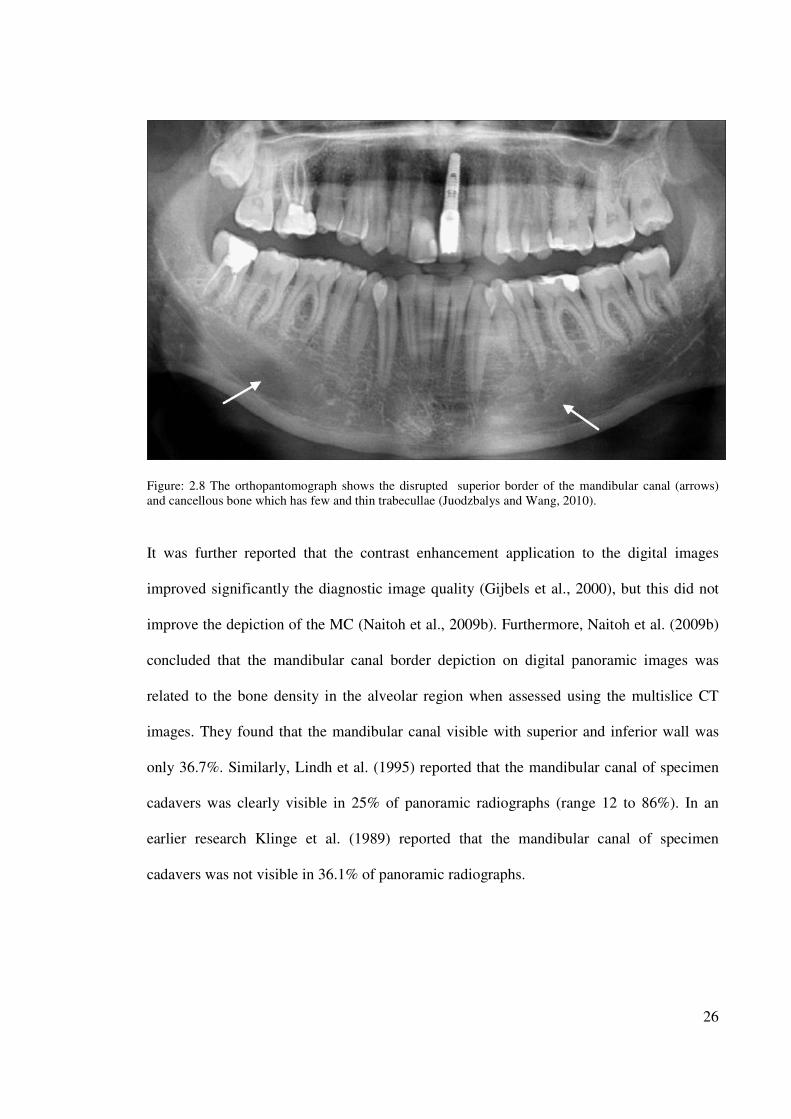
Wadu et al. (1997) employed panoramic radiographs to study the mandibular canal
appearance and they found that in number of cases the radio-opaque border was either
disrupted or even absent. The superior border was more prone to disruption than the
inferior border (Figure 2.8).
26
Figure: 2.8 The orthopantomograph shows the disrupted superior border of the mandibular canal (arrows)
and cancellous bone which has few and thin trabecullae (Juodzbalys and Wang, 2010).
It was further reported that the contrast enhancement application to the digital images
improved significantly the diagnostic image quality (Gijbels et al., 2000), but this did not
improve the depiction of the MC (Naitoh et al., 2009b). Furthermore, Naitoh et al. (2009b)
concluded that the mandibular canal border depiction on digital panoramic images was
related to the bone density in the alveolar region when assessed using the multislice CT
images. They found that the mandibular canal visible with superior and inferior wall was
only 36.7%. Similarly, Lindh et al. (1995) reported that the mandibular canal of specimen
cadavers was clearly visible in 25% of panoramic radiographs (range 12 to 86%). In an
earlier research Klinge et al. (1989) reported that the mandibular canal of specimen
cadavers was not visible in 36.1% of panoramic radiographs.
27
According to Vazquez et al.(2008), if a safety margin of at least 2 mm above the
mandibular canal is ascertained, panoramic radiography appears to be sufficient to evaluate
available bone height prior to insertion of posterior mandibular implants; cross-sectional
imaging techniques may not be necessary.
Panoramic radiographs can be predictably used for visualization of the mental foramen and
a potential anterior looping but not suitable for locating the mandibular incisive canal. To
verify its existence for preoperative planning purposes, cross-sectional imaging modalities
such as high resolution computed tomography (HR-CT) or spiral tomography, and CBCT
should be preferred. High resolution magnetic resonance imaging (HR-MRI) is not
preferred due to the high cost of this machine.
2.6.3 Conventional tomography
Tomography word was derived from the Greek word “tomos” which means "a section", "a
slice" or "a cutting". In conventional tomography, different types of motion of the x-ray
tube and the film are employed. They are linear, circular, trispiral, elliptical, and
hypocycloidal, the simplest of the motions being linear. The more complex the motion is,
the sharper the image. There is always some degree of blurring in tomography, the greatest
amount of blurring being at the periphery. This modality has now become obsolete.
28
2.6.4. Computed tomography (CT)
Computerized tomography, unlike the conventional radiological technique, enables the 3D
evaluation of the bone without the overlapping of the adjacent structure, as well as a precise
measurement of the bone tissue availability.
CT was introduced in imaging the maxillofacial structure in the early 1970's. It was
considerably developed after the introduction of dental implantology, when the need
increased for advanced radiologic procedures to document the availability or
nonavailability of bone and to identify important anatomic structures such as the
mandibular canal.
The obtained CT data can be manipulated and reconstructed with a software program such
as DentaScan or SimPlant. Interpretation of these processed images is much easier, accurate
and may reveal most of the relevant structures such as accessory canals and foramen which
are occupied by neurovascular bundles, arterioles and venules.
CT images are produced by x-ray beams that penetrate patients to varying degrees and
strike a detector. The generation of the scan is determined by the placement of the x-ray
tube relative to the detectors. The entire CT process is divided into three segments: data
acquisition, image reconstruction and image display. Raw data include all measurements
obtained from the detector array. After the raw data is averaged and each pixel is assigned a
CT number (quantified measurement of density), an image can be reconstructed. The data
that form this image is then referred as image data (Gultekin et al., 2003).
29
In a study done by Yang et al.(1999), employed a spiral computed tomography machine to
scan on four edentulous cadaver heads with intact mandible. They wanted to find out if
there were any statistically significant differences between the 2D computed tomography
measurements and the physical measurements or between the 3D computed tomography
measurements and the physical measurements. The data were then transferred to third party
software - Radredux to generate 2D and 3D images. Linear measurements of the images
were made from the superior border of the inferior alveolar canal to the alveolar crest. The
specimens were then dissected at corresponding locations, and physical measurements were
made. It was concluded that 2D and 3D computed tomography images allowed accurate
measurements for localization of the inferior alveolar canal.
CT values (Hounsfield units: HU) and bone mineral densities obtained by medical CT were
used to assess the bone density of jaws. Norton and Gamble (2001) measured the bone
density in the posterior mandible using SimPlant software (3D Diagnostix, Boston, MA,
USA) and concluded that the mean CT value was 669.6 HU. (Misch, 1999).
Another attempt to improve depiction of the mandibular canal was by changing the
thickness of double-oblique computed tomography images (Naitoh et al., 2008). A total of
38 sites in the mandibular molar region were examined using multislice helical CT. The
thicknesses of the double-oblique images using multislice helical CT scans were
reconstructed in 4 conditions: 0.3 mm, 0.9 mm, 1.6 mm, and 4.1 mm. In the alveolar crest
and the entire mandibular canal, highest value was obtained with 0.9 mm thick images;
however, there was no significant difference between 0.3 mm and 0.9 mm thick images.
The researchers then concluded that the description of superior wall of MC cannot be
improved by changing the thickness of images.
30
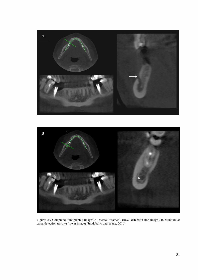
However, the measurements obtained from computed tomographic images are more
consistent with direct measurements than the measurements obtained from panoramic
radiographic images or conventional tomographic images (Figure 2.9 A and B). This
conclusion was made by Peker et al. (2008) after the comparison of efficiency of panoramic
radiographs, conventional tomograms, and computed tomograms for location of the
mandibular canal at 12 regions of 6 dry adult human skulls. Furthermore, Rouas et al.
(2007) reported that the atypical mandibular canal (such as bifid MC). In most cases can be
identified using only three-dimensional imaging techniques. Therefore it is reported that the
bifid MC is often left unrecognized (Claeys and Wackens, 2005).
31
Figure: 2.9 Computed tomographic images A. Mental foramen (arrow) detection (top image). B. Mandibular
canal detection (arrow) (lower image) (Juodzbalys and Wang, 2010).
A
B
32
2.7 Studies locating the mandibular canal preoperatively
The earlier study made to determine the vertical location of the mandibular canal was
mostly based on cadaver studies (Carter and Keen, 1971, Tamas, 1987, Gowgiel, 1992).
There were also radiographic studies (Nortjĕ et al., 1977b, Heasman, 1988, Fox, 1989) that
disclosed the position of the mandibular canal adjacent to the apices of the teeth, but could
not determine if the canal is buccal or lingual to the teeth. However, some radiographic
methods have been used to locate the mandibular canal buccolingually, mostly before the
implant surgery (Rothman et al., 1988, Klinge et al., 1989, Lindh and Petersson, 1989,
Jacobs et al., 1999, Yang et al., 1999, Hallikainen et al., 1992).
It has been assumed that in areas where the neurovascular bundle is in contact with either
the buccal or lingual cortex, the mandibular canal is well visualized in radiographs (Miller
et al., 1990) and it is suggested that cortication of the mandibular canal on the panoramic
film may serve as a predictor of the proximity of the mandibular canal to the cortical plates.
The anatomic features of the ascent or descent of the canal, as well as its buccolingual
relationships, have been studied by Mercier (1973), Tamas (1987) and Gowgiel (1992).
According to the report by Gowgiel on dissections of the IAN, the neurovascular bundle
from the mandibular foramen to the mental foramen is always in contact with, or in close
proximity to the lingual mandibular cortex. Furthermore, the rnandibular canal ascends
slightly toward the mental foramen in the anterior mandible. However, it has been shown,
that vascular and nerve bundles may also be extremely close to the buccal cortex of the
mandible in broad and thick mandibular rami. The study of Rajchel et al. (1986) on 45
Asian adults demonstrated that the mandibular canal when proximal to the third-molar
region is usually a single large structure (2.0 to 2.4 mm in diameter). It courses
33
approximately 2.0 mm from the inner lingual cortex, 1.6 to 2.0 mm from the medial aspect
of the buccal plate, and about 10 mm from the inferior border.
A study done by Lindh et al. (1992), employed visualization of the mandibular canal by
five different radiographic techniques: periapical radiography, panoramic radiography,
hypocycloidal tomography, spiral tomography and computerized tomography. They noticed
that direct CT demonstrated the mandibular canal best of the examined techniques, and it
also gave a high inter- and intraobserver agreement rate. This was supported by Sonic et
al.(1994) on the accuracy of periapical, panoramic, and computerized tomographic
radiographs in locating the mandibular canal. They too found CT to be superior to the other
techniques in locating the mandibular canal.
Comparing the tomographic techniques with panoramic radiography, Tal and Moses (1991)
reported that CT-scans have again been found to be more precise in measuring the distance
between the bony crest and the mandibular canal compared to panoramic radiography. In
addition, the tomographic radiographs have an additional advantage in presurgical planning
as they reveal the horizontal dimension, shape of the mandible and the topography and
buccolingual location of the mandibular canal.
A study was performed by Ylikontiola et al.(2002) to compare three radiographic
techniques to locate the mandibular canal in the buccolingual direction before BSSO.
Panoramic radiographs, computerized tomography (CT) and conventional spiral
tomographic (Scanora, Soredex, Helsinki, Finland) radiographs were compared for their
ability to localize the mandibular canal in the buccolingual direction. The subjective
neurosesnsory deficit of the lower lip and chin on both sides was registered preoperatively
34
at 4 days, 3 weeks, and 3 months after surgery, and the operative outcome was analyzed in
relation to the distance from the mandibular canal to the buccal cortex of the mandible.
Computed tomography gave better visualization of the mandibular canal than Scanora
imaging. Cortication of the mandibular canal on the panoramic radiograph did not serve as
a predictor of the proximity of the mandibular canal to the cortices of the mandible. At 3-
month follow-up, there were only eight operated sides with abnormal sensation of the lower
lip and chin. In seven of these sides, the distance from the mandibular canal to the buccal
cortex was less than 2 mm using CT technique. As a conclusion, The buccolingual location
of the mandibular canal is visualized better with CT than with Scanora or panoramic
radiographs.
Klinge et al.(1989) radiographically examined four mandibular specimens bilaterally to
locate the mandibular canal. The following radiographic techniques were used: periapical
and panoramic radiography, hypocycloidal tomography, and computed tomography (CT).
The distance from the crest of the alveolar process to the superior border of the mandibular
canal was measured in millimeters on all radiographs. The specimens were then sectioned,
and the location of the mandibular canal (as measured on contact radiographs of the
sections) was compared with measurements made on the other radiographs. The results
showed that CT gave the most accurate position of the mandibular canal and is therefore
probably the best method for preoperative planning of the implant surgery involving the
area close to the mandibular canal.
Lindh et al.(1992) radiographically examined six mandibles bilaterally to visualize the
mandibular canal. Five imaging techniques were used: periapical radiography, panoramic
radiography, hypocydoidal tomography, spiral tomography and computed tomography
35
(CT). Panoramic radiographs were obtained with 2 different X-ray machines. The CT-
examinations comprised direct images and standard reconstruction based on axial slices.
The specimens were subsequently sectioned for contact radiography. The visibility of the
mandibular canal was estimated by 3 observers at special reference points on all
radiographs and classified as clearly visible, questionable visibility or not visible. The
contact radiographs served as the "gold standard". The inter-observer and the intra-observer
agreement were assessed by calculating the overall agreement and the x value. Direct
coronal computed tomography, as well as spiral and hypocycloidal tomography, gave better
visualisation of the mandibular canal than periapical and panoramic radiography.
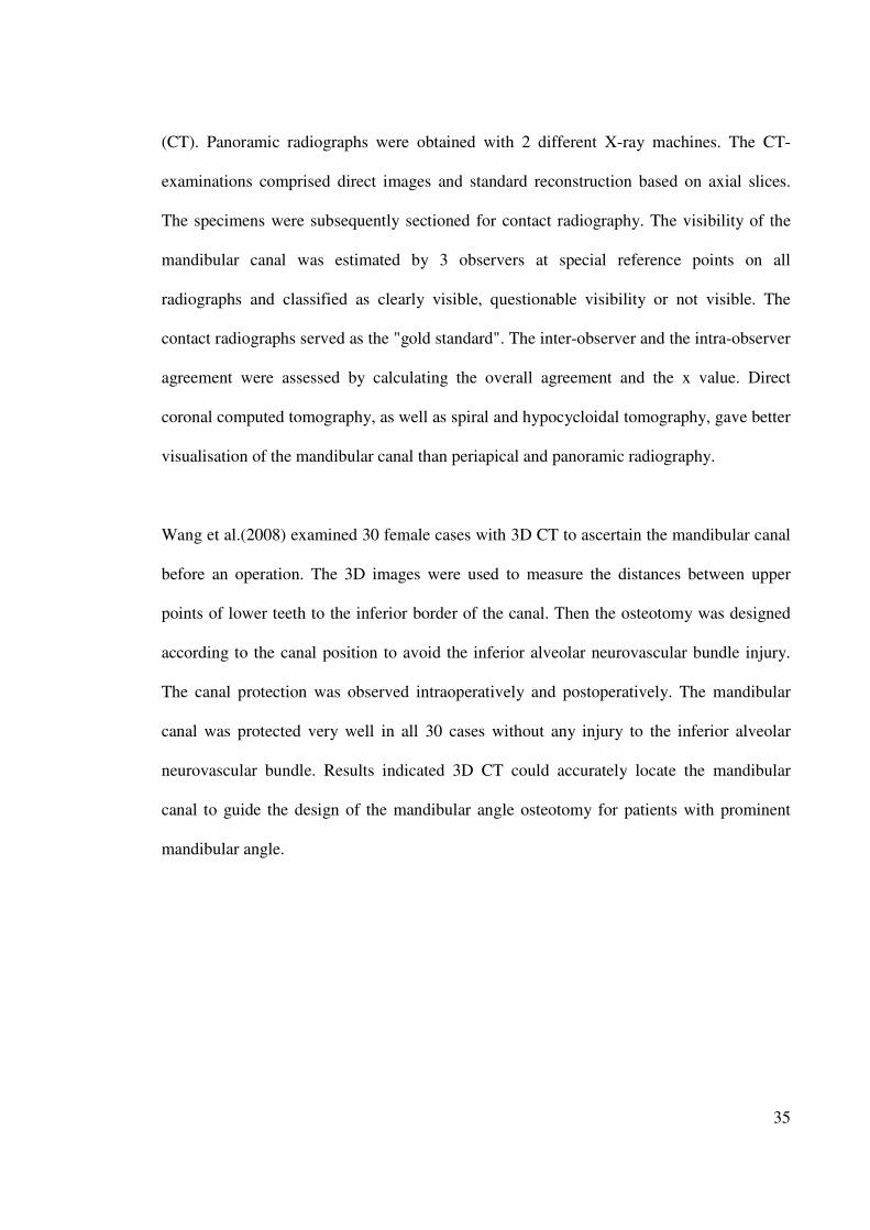
Wang et al.(2008) examined 30 female cases with 3D CT to ascertain the mandibular canal
before an operation. The 3D images were used to measure the distances between upper
points of lower teeth to the inferior border of the canal. Then the osteotomy was designed
according to the canal position to avoid the inferior alveolar neurovascular bundle injury.
The canal protection was observed intraoperatively and postoperatively. The mandibular
canal was protected very well in all 30 cases without any injury to the inferior alveolar
neurovascular bundle. Results indicated 3D CT could accurately locate the mandibular
canal to guide the design of the mandibular angle osteotomy for patients with prominent
mandibular angle.
36
2.8 Cone Beam Computed Tomography (CBCT) in dentistry
CBCT Scanners have been available for craniofacial imaging since 1999 in Europe, 2001 in
the United States, and 2005 in Australia. Although the imaging was created using computed
tomography (CT) and appear similar to conventional medical multislice CT (MSCT)
images, the method of x-ray emission and capture is quite different.
CBCT imaging technique is considered as one of the many new imaging modalities and
techniques that have changed the way we approach dental diagnosis and treatment
planning, particularly when anatomy of the maxillofacial complex is of paramount
importance.
The introduction of Cone Beam Computed Tomography (CBCT) in 1998 has completely
revolutionized the imaging modalities in dentistry and has changed the practice of oral and
maxillofacial radiology and orthodontics (Ludlow et al., 2006).
CBCT produces 3D images of the bony structure being scanned, which has applied in
various areas of dentistry such as assessment of tooth impaction, paranasal sinus evaluation,
trauma evaluation, temporomandibular joint visualization; surgical guide fabrication,
implantology, endodontics and craniofacial surgery assessments and visualization of the
anatomy of the mandibular canal.
Whether we are looking at the position of the canal with respect to third molar, or treatment
planning for implants, viewing the mandible in all three dimensions helps us extract the
maximum information needed for diagnosis and treatment.
37
CBCT is capable of providing sub-millimeter resolution in images of high diagnostic
quality, with short scanning time about 10-70 seconds and radiation dosages reportedly up
to 15 times lower than those of conventional CT scan (Scarfe et al., 2006)
According to Sukovic (2003), CBCT can be combined with application-specific software
tools can provide dentomaxillofacial practitioners with a complete solution for performing
specific diagnostic and surgical tasks, such as dental implant planning, temporomandibular
joint imaging, detection of facial fractures, lesions and diseases of soft tissue in the head
and neck as well as in reconstructive facial surgery.
For most dental practitioners, the use of advanced imaging has been limited because of
cost, availability and radiation dose considerations. However, the introduction of CBCT for
maxillofacial region provides an opportunity for surgeons to request for multiplanar
imaging.
CBCT allows the creation in "real time" of the images not only in the axial plane but also 2-
dimensional (2D) images in the coronal, sagittal, oblique or curved image planes a process
known as Multiplanar reformation (MPR). In addition, CBCT data are amenable to the
reformation in a volume, rather than slice, providing three dimensional (3D) information
(Scarfe et al., 2006).
38
Figure 2.10: Cone beam computed tomography system showing the x-ray source (to the left of the model) and
the receptor (Lam, 2007).
Figure 2.11: Illustrated diagrams for x-ray cone beam emission and detection. 2.11A show the fan
beam on which spiral computed tomography (left) is based interrogates only a slice of tissue,
whereas the cone-beam of cone-beam computed tomography (right) interrogates a 3-dimensional
region within a 360° rotation. 2.11B diagram show Cone-beam computed tomography reconstructs
the 3-dimensional images by generating voxel directly, each with its own attenuation coefficient
(MacDonald-Jankowski and Orpe, 2007).
2.11A 2.11B
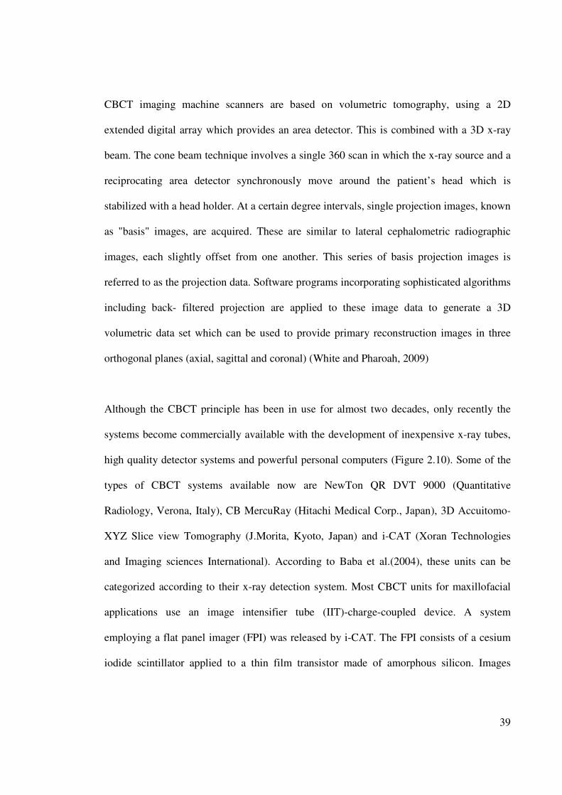
39
CBCT imaging machine scanners are based on volumetric tomography, using a 2D
extended digital array which provides an area detector. This is combined with a 3D x-ray
beam. The cone beam technique involves a single 360 scan in which the x-ray source and a
reciprocating area detector synchronously move around the patient’s head which is
stabilized with a head holder. At a certain degree intervals, single projection images, known
as "basis" images, are acquired. These are similar to lateral cephalometric radiographic
images, each slightly offset from one another. This series of basis projection images is
referred to as the projection data. Software programs incorporating sophisticated algorithms
including back- filtered projection are applied to these image data to generate a 3D
volumetric data set which can be used to provide primary reconstruction images in three
orthogonal planes (axial, sagittal and coronal) (White and Pharoah, 2009)
Although the CBCT principle has been in use for almost two decades, only recently the
systems become commercially available with the development of inexpensive x-ray tubes,
high quality detector systems and powerful personal computers (Figure 2.10). Some of the
types of CBCT systems available now are NewTon QR DVT 9000 (Quantitative
Radiology, Verona, Italy), CB MercuRay (Hitachi Medical Corp., Japan), 3D Accuitomo-
XYZ Slice view Tomography (J.Morita, Kyoto, Japan) and i-CAT (Xoran Technologies
and Imaging sciences International). According to Baba et al.(2004), these units can be
categorized according to their x-ray detection system. Most CBCT units for maxillofacial
applications use an image intensifier tube (IIT)-charge-coupled device. A system
employing a flat panel imager (FPI) was released by i-CAT. The FPI consists of a cesium
iodide scintillator applied to a thin film transistor made of amorphous silicon. Images
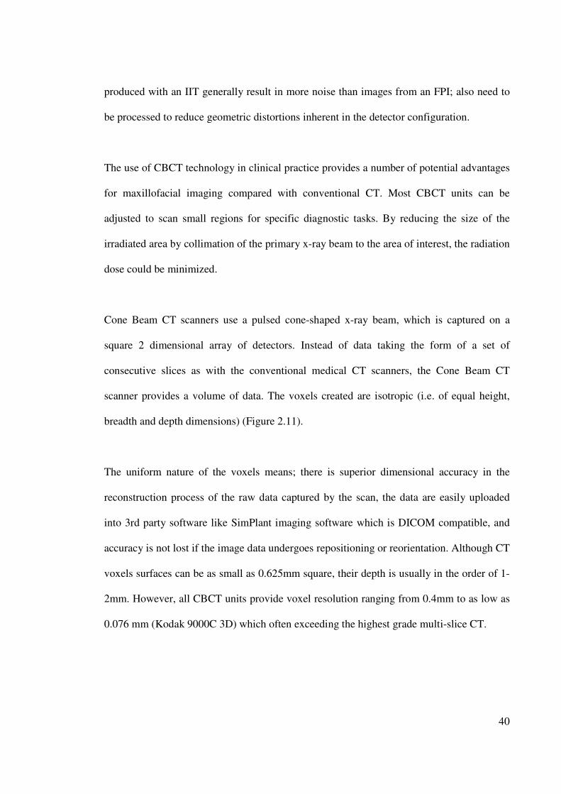
40
produced with an IIT generally result in more noise than images from an FPI; also need to
be processed to reduce geometric distortions inherent in the detector configuration.
The use of CBCT technology in clinical practice provides a number of potential advantages
for maxillofacial imaging compared with conventional CT. Most CBCT units can be
adjusted to scan small regions for specific diagnostic tasks. By reducing the size of the
irradiated area by collimation of the primary x-ray beam to the area of interest, the radiation
dose could be minimized.
Cone Beam CT scanners use a pulsed cone-shaped x-ray beam, which is captured on a
square 2 dimensional array of detectors. Instead of data taking the form of a set of
consecutive slices as with the conventional medical CT scanners, the Cone Beam CT
scanner provides a volume of data. The voxels created are isotropic (i.e. of equal height,
breadth and depth dimensions) (Figure 2.11).
The uniform nature of the voxels means; there is superior dimensional accuracy in the
reconstruction process of the raw data captured by the scan, the data are easily uploaded
into 3rd party software like SimPlant imaging software which is DICOM compatible, and
accuracy is not lost if the image data undergoes repositioning or reorientation. Although CT
voxels surfaces can be as small as 0.625mm square, their depth is usually in the order of 1-
2mm. However, all CBCT units provide voxel resolution ranging from 0.4mm to as low as
0.076 mm (Kodak 9000C 3D) which often exceeding the highest grade multi-slice CT.
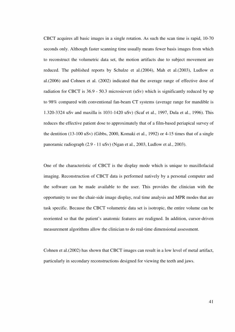
41
CBCT acquires all basic images in a single rotation. As such the scan time is rapid, 10-70
seconds only. Although faster scanning time usually means fewer basis images from which
to reconstruct the volumetric data set, the motion artifacts due to subject movement are
reduced. The published reports by Schulze et al.(2004), Mah et al.(2003), Ludlow et
al.(2006) and Cohnen et al. (2002) indicated that the average range of effective dose of
radiation for CBCT is 36.9 - 50.3 microsievert (uSv) which is significantly reduced by up
to 98% compared with conventional fan-beam CT systems (average range for mandible is
1.320-3324 uSv and maxilla is 1031-1420 uSv) (Scaf et al., 1997, Dula et al., 1996). This
reduces the effective patient dose to approximately that of a film-based periapical survey of
the dentition (13-100 uSv) (Gibbs, 2000, Komaki et al., 1992) or 4-15 times that of a single
panoramic radiograph (2.9 - 11 uSv) (Ngan et al., 2003, Ludlow et al., 2003).
One of the characteristic of CBCT is the display mode which is unique to maxillofacial
imaging. Reconstruction of CBCT data is performed natively by a personal computer and
the software can be made available to the user. This provides the clinician with the
opportunity to use the chair-side image display, real time analysis and MPR modes that are
task specific. Because the CBCT volumetric data set is isotropic, the entire volume can be
reoriented so that the patient’s anatomic features are realigned. In addition, cursor-driven
measurement algorithms allow the clinician to do real-time dimensional assessment.
Cohnen et al.(2002) has shown that CBCT images can result in a low level of metal artifact,
particularly in secondary reconstructions designed for viewing the teeth and jaws.
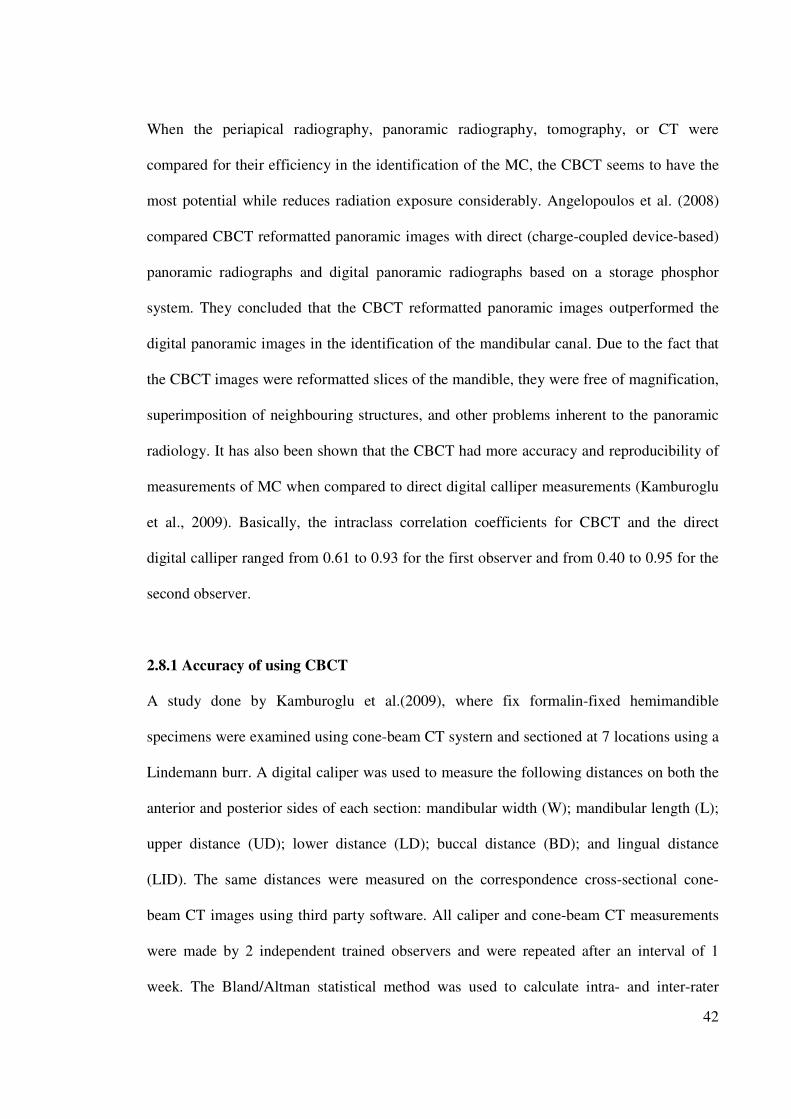
42
When the periapical radiography, panoramic radiography, tomography, or CT were
compared for their efficiency in the identification of the MC, the CBCT seems to have the
most potential while reduces radiation exposure considerably. Angelopoulos et al. (2008)
compared CBCT reformatted panoramic images with direct (charge-coupled device-based)
panoramic radiographs and digital panoramic radiographs based on a storage phosphor
system. They concluded that the CBCT reformatted panoramic images outperformed the
digital panoramic images in the identification of the mandibular canal. Due to the fact that
the CBCT images were reformatted slices of the mandible, they were free of magnification,
superimposition of neighbouring structures, and other problems inherent to the panoramic
radiology. It has also been shown that the CBCT had more accuracy and reproducibility of
measurements of MC when compared to direct digital calliper measurements (Kamburoglu
et al., 2009). Basically, the intraclass correlation coefficients for CBCT and the direct
digital calliper ranged from 0.61 to 0.93 for the first observer and from 0.40 to 0.95 for the
second observer.
2.8.1 Accuracy of using CBCT
A study done by Kamburoglu et al.(2009), where fix formalin-fixed hemimandible
specimens were examined using cone-beam CT systern and sectioned at 7 locations using a
Lindemann burr. A digital caliper was used to measure the following distances on both the
anterior and posterior sides of each section: mandibular width (W); mandibular length (L);
upper distance (UD); lower distance (LD); buccal distance (BD); and lingual distance
(LID). The same distances were measured on the correspondence cross-sectional cone-
beam CT images using third party software. All caliper and cone-beam CT measurements
were made by 2 independent trained observers and were repeated after an interval of 1
week. The Bland/Altman statistical method was used to calculate intra- and inter-rater
43
reliability. Intra-class correlation coefficients (ICCs) from 2-way random effects model
were calculated. Agreements between cone-beam CT and direct digital caliper were
calculated by ICC for 6 distances and 2 observers.
Intraobserver and interobserver measurements for all distance showed high agreement.
ICCs for intraobserver agreement ranged from 0.86 to 0.97 for cone-beam CT
measurements and from 0.98 to 0.99 for digital caliper measurements. ICCs between
observers ranged from 0.84 to 0.97 for the cone-beam CT measurements and from 0.78 to
0.97 for the digital caliper measurements. ICCs for cone-beam CT and direct digital caliper
ranged from 0.61 to 0.93 for the first observer and from 0.40 to 0.95 for the second
observer.
As a conclusion, accuracy of cone-beam CT measurements of various distances
surrounding the mandibular canal was comparable to that of direct digital caliper
measurements.
Another study by Angelopoulos et al.(2008), where panoramic images, generated by 3
different imaging modalities used for general rnaxillofacial diagnosis and preimplant
assessment, were compared: (a) CBCT reformatted panoramic images (I-CAT; Imaging
Sciences, Hatfield, PA), (b) Direct (charge-coupled device-based) panoramic radiographs
(DIMAX; Planmeca, Helsinki, Finland), and (c) digital panoramic radiographs based on a
storage phosphor system (DENOPTIX; Gendex, Chicago, IL). Three independent groups of
images were used (40 in each group) from patients examined by one of the above imaging
modalities over a period of 6 months. In total, 68 randomly selected mandibular canals (out
of a possible 80) per imaging modality were evaluated. Four experienced raters evaluated
44
the images of each modality in 3 sessions under standardized conditions for clarity in the
visualization of the mandibular canal in 3 locations, using a 4-point scale. As as result
CBCT reformatted panoramic images outperformed the digital panoramic images in the
identification of the mandibular canal.
Another study was made by (Tantanapornkul et al., 2007) to compare the diagnostic
accuracy of cone-beam computed tomography and conventional panoramic radiography in
assessing the topographic relationship between the mandibular canal and impacted third
molars. One hundred and forty two impacted mandibular third molars were evaluated to
assess tooth relationship to the mandibular canal. The sensitivity and specificity of the 2
modalities in predicting neurovascular bundle exposure at extraction were calculated and
compared. The sensitivity and specificity were 93% and 77% for cone-beam CT, and 70%
and 63% for panoramic images, respectively. As a result cone-beam CT was significantly
superior to panoramic images in predicting neurovascular bundle exposure during
extraction of impacted mandibular third molar teeth.
2.8.2 Image quality of CBCT
Brooks et al.(2004) conducted research on five unembalmed cadaver heads and three living
humans head employing cone-beam CT scanner (I-CAT) using default parameters to
evaluate identification of the mandibular canal. The latter can be seen easily in living
human scan but was not readily visible on scans of cadavers. This suggests that factors such
as the age of the specimens and the effect of the thawing process must be taken in
consideration when evaluating image quality.
45
Neugebauer et al. (2008) reported that panoramic radiograph and symmetrical panoramic
cephalometric radiograph (PAN&PA) was compared with that of a cone-beam volumetric
imaging (CBCT) device. Thirteen cases were evaluated by PAN&PA and the same thirteen
cases evaluated via CBCT for the position of root tips of third molar. Cone Beam
technology actually improved the localization of third molar for presurgical planning.
Kobayashi et al.(2004) examined five cadaver mandibles by spiral computerized
tomography (SCT) and cone-beam computed tomography to evaluate the accuracy of
measurement of distance on the images produced by computerized tomography. The
vertical distance from a reference point to the alveolar ridge was measured by caliper on the
sliced mandible, and measurement error on the CT images was calculated in percentages
based on the actual values and the measurement values obtained from the CT images.
Measurement error was determined to range from 0 to 1.11 mm (0% to 6.9%) on SCT and
from 0.01 to 0.65 mm (0.1% to 5.2%) on CBCT, with measurement errors of 2.2% and
1.4%, respectively (P < .0001). There is significance in the difference observed with the
two modalities.
This research showed that using CBCT is a useful tool for preoperative evaluation
compared to SCT, However it is able to collimate the field size and thereby reducing the
exposure to ionizing X-ray radiation.
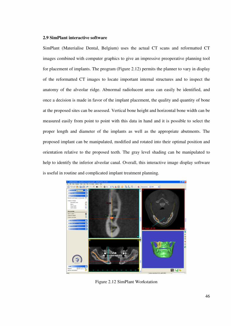
46
2.9 SimPlant interactive software
SimPlant (Materialise Dental, Belgium) uses the actual CT scans and reformatted CT
images combined with computer graphics to give an impressive preoperative planning tool
for placement of implants. The program (Figure 2.12) permits the planner to vary in display
of the reformatted CT images to locate important internal structures and to inspect the
anatomy of the alveolar ridge. Abnormal radiolucent areas can easily be identified, and
once a decision is made in favor of the implant placement, the quality and quantity of bone
at the proposed sites can be assessed. Vertical bone height and horizontal bone width can be
measured easily from point to point with this data in hand and it is possible to select the
proper length and diameter of the implants as well as the appropriate abutments. The
proposed implant can be manipulated, modified and rotated into their optimal position and
orientation relative to the proposed teeth. The gray level shading can be manipulated to
help to identify the inferior alveolar canal. Overall, this interactive image display software
is useful in routine and complicated implant treatment planning.
Figure 2.12 SimPlant Workstation
47
CHAPTER 3
RESEARCH MEHODOLOGY
3.1 Introduction
The present research study was designed to analyze metrically the course of the mandibular
canal for dentate patients among Malaysian population in posterior part of the mandible
using Cone Beam Computed Tomography (CBCT) and SimPlant interactive software.
3.2 The materials of the study
Cone Beam Computed Tomography images taken using I-CAT CBCT system at the
Division of Oral Radiology, Faculty of Dentistry, University of Malaya, Kuala Lumpur,
Malaysia were used. The relevant data was downloaded and saved in an external hard disc
for the purpose of this study.
Latest CBCT records taken shall be the priority of selection; starting from records in the
month of January 2010 and moving backwards in time until adequate number of patients
were selected. Out of more than one hundred records retrieved from February 2007 to
January 2010 and 60 suitable cases were used for this study.
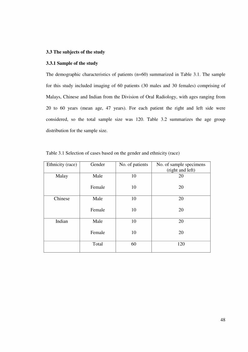
48
3.3 The subjects of the study
3.3.1 Sample of the study
The demographic characteristics of patients (n=60) summarized in Table 3.1. The sample
for this study included imaging of 60 patients (30 males and 30 females) comprising of
Malays, Chinese and Indian from the Division of Oral Radiology, with ages ranging from
20 to 60 years (mean age, 47 years). For each patient the right and left side were
considered, so the total sample size was 120. Table 3.2 summarizes the age group
distribution for the sample size.
Table 3.1 Selection of cases based on the gender and ethnicity (race)
Ethnicity (race) Gender No. of patients No. of sample specimens
(right and left)
Malay Male
Female
10
10
20
20
Chinese Male
Female
10
10
20
20
Indian Male
Female
10
10
20
20
Total 60 120
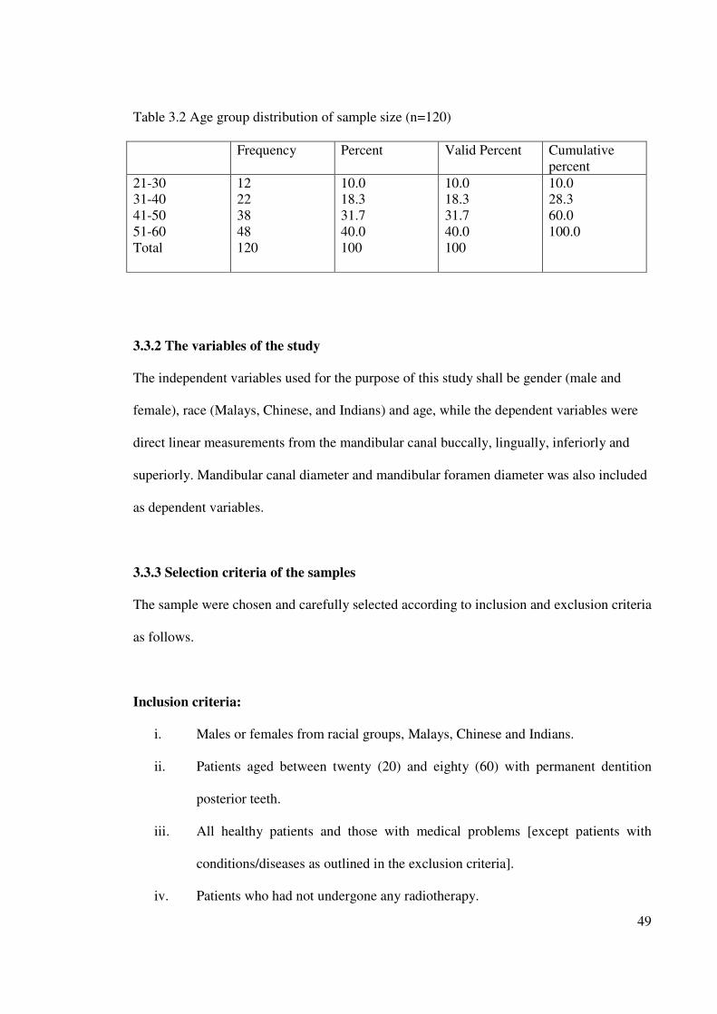
49
Table 3.2 Age group distribution of sample size (n=120)
Frequency Percent Valid Percent Cumulative
percent
21-30
31-40
41-50
51-60
Total
12
22
38
48
120
10.0
18.3
31.7
40.0
100
10.0
18.3
31.7
40.0
100
10.0
28.3
60.0
100.0
3.3.2 The variables of the study
The independent variables used for the purpose of this study shall be gender (male and
female), race (Malays, Chinese, and Indians) and age, while the dependent variables were
direct linear measurements from the mandibular canal buccally, lingually, inferiorly and
superiorly. Mandibular canal diameter and mandibular foramen diameter was also included
as dependent variables.
3.3.3 Selection criteria of the samples
The sample were chosen and carefully selected according to inclusion and exclusion criteria
as follows.
Inclusion criteria:
i. Males or females from racial groups, Malays, Chinese and Indians.
ii. Patients aged between twenty (20) and eighty (60) with permanent dentition
posterior teeth.
iii. All healthy patients and those with medical problems [except patients with
conditions/diseases as outlined in the exclusion criteria].
iv. Patients who had not undergone any radiotherapy.

50
Exclusion criteria:
i. Individuals with mixed racial origin.
ii. Patients with history of trauma or fracture of the mandible.
iii. Patients with existing pathological disorder at mandible such as cyst, tumor,
osteomyelitis, fibrous dysplacia etc.
iv. Patients with genetic disorder or congenital abnormalities.
v. Post-surgical cases such as orthognathic surgery, sagital split osteotomy,
apicectomy and placement of endosseous oral implants.
vi. The reformatted CBCT images which appear distorted or blurred with artifacts
due to (1) presence of metal within the jaw or teeth, (2) those resulting from
patient motion, and (3) due to improperly angled CBCT scan.
vii. Very osteoporotic demineralized mandible which makes it difficult to
distinguish the canal and the medullary bone.
viii. Severely atrophied mandible.
51
3.4 Methodology
3.4.1 Methods
The selected samples from the CBCT data were stored in an external hard disk. They were
then transferred to a workstation for further processing. The images were reformatted using
SimPlant software version 13 from Materialise lnc. The SimPlant software allows viewing
of axial, cross-sectional, Panoramic and 3D visualization of the jaw on the same screen.
The SimPlant workstation is most outstanding for the three dimensional renderings. This
workstation is capable of displaying an entire volume of data from a large number of
angles. It therefore allows the operator to define the picture elements that make up the
osseous structures. In the 3D visualization, the jaw can be turned in space, rotated or spun
360 degrees and viewed from any angle.
The vital structures such as inferior alveolar nerve can be colored and displayed through the
bone as if the bone were transparent (Figure 3.1).
For this research, the anatomy of the whole mandible was assessed first in the axial, coronal
and panoramic views. Then the mandibular canal was examined and verified in all three
planes.
The SimPlant software tool allow the marking to be done in any of the axial, cross
sectional, Panoramic or 3D views and it will be simultaneously displayed in all four views
on the screen. As such, this fully integrated planning tool allows identification of the canals
with unparallel precision and at the same time provides 3D digital visualization of the jaw
and canals.
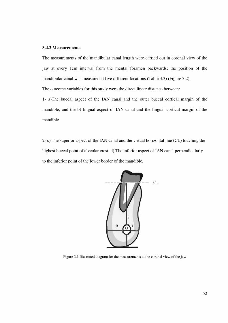
52
3.4.2 Measurements
The measurements of the mandibular canal length were carried out in coronal view of the
jaw at every 1cm interval from the mental foramen backwards; the position of the
mandibular canal was measured at five different locations (Table 3.3) (Figure 3.2).
The outcome variables for this study were the direct linear distance between:
1- a)The buccal aspect of the IAN canal and the outer buccal cortical margin of the
mandible, and the b) lingual aspect of IAN canal and the lingual cortical margin of the
mandible.
2- c) The superior aspect of the IAN canal and the virtual horizontal line (CL) touching the
highest buccal point of alveolar crest .d) The inferior aspect of IAN canal perpendicularly
to the inferior point of the lower border of the mandible.
Figure 3.1 Illustrated diagram for the measurements at the coronal view of the jaw
CL
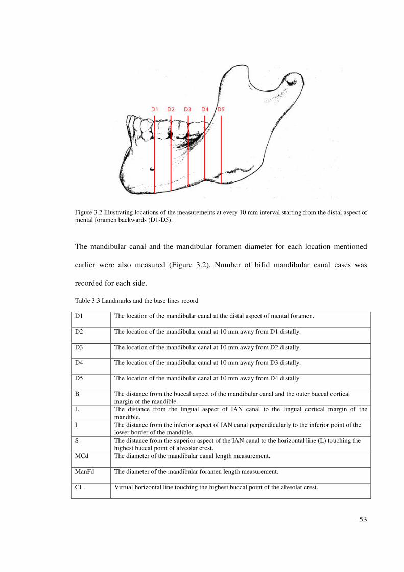
53
Figure 3.2 Illustrating locations of the measurements at every 10 mm interval starting from the distal aspect of
mental foramen backwards (D1-D5).
The mandibular canal and the mandibular foramen diameter for each location mentioned
earlier were also measured (Figure 3.2). Number of bifid mandibular canal cases was
recorded for each side.
Table 3.3 Landmarks and the base lines record
D1 The location of the mandibular canal at the distal aspect of mental foramen.
D2 The location of the mandibular canal at 10 mm away from D1 distally.
D3 The location of the mandibular canal at 10 mm away from D2 distally.
D4 The location of the mandibular canal at 10 mm away from D3 distally.
D5 The location of the mandibular canal at 10 mm away from D4 distally.
B The distance from the buccal aspect of the mandibular canal and the outer buccal cortical
margin of the mandible.
L The distance from the lingual aspect of IAN canal to the lingual cortical margin of the
mandible.
I The distance from the inferior aspect of IAN canal perpendicularly to the inferior point of the
lower border of the mandible.
S The distance from the superior aspect of the IAN canal to the horizontal line (L) touching the
highest buccal point of alveolar crest.
MCd The diameter of the mandibular canal length measurement.
ManFd The diameter of the mandibular foramen length measurement.
CL Virtual horizontal line touching the highest buccal point of the alveolar crest.
54
3.4.3 Reliability of the measurement
Since the research consist of huge number of details of quantitative data, the intraexaminer
reliability and reproducibility of the measurements obtained were evaluated. A total number
of twelve patients’ records which is actually 20% of the sample size were randomly
selected (two patients from each race and gender group) and all the data were measured
again after three weeks using same methods described previously.
The consistency of data was analyzed and the Cronbach alpha coefficient was calculated
for all the measured data.
3.5 Data analysis
All calculations and measurements were processed using SPSS statistical software version
12. The measured values for right and left mandible, gender, race and age were computed
using appropriate statistical analysis. Figure 3.3 summarizes the methodology of this study.
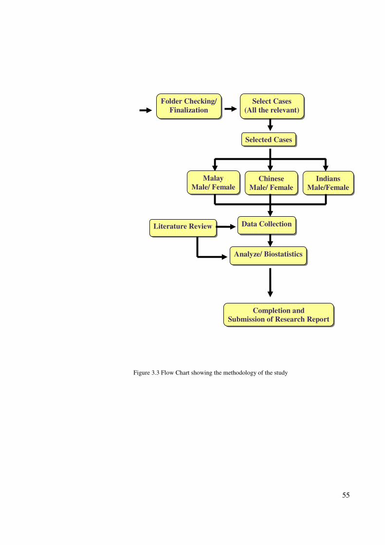
55
Figure 3.3 Flow Chart showing the methodology of the study
Selected Cases
Folder Checking/
Finalization
Select Cases
(All the relevant)
Malay
Male/ Female Chinese
Male/ Female
Indians
Male/Female
Literature Review Data Collection
Analyze/ Biostatistics
Completion and
Submission of Research Report
56
CHAPTER 4
RESULTS AND DATA ANALYSIS
4.1 Introduction
This study analyzes the path and course of the mandibular canal of dentate patient at 5
locations starting from mental foramen backward at 10 mm interval. It also measures the
mandibular canal and mandibular foremen diameter, and indicates the frequency of bifid
mandibular canal among Malaysian population.
This chapter discusses the results of the study. The analysis and its interpretation for MC
course were organized from D1-D5 (Figure 4.1). For each D location there were 4 aspects
considered which are the measurements observed buccally, lingually, inferiorly and
superiorly respectively (with exception of the measurements at D5S location).
Subsequently the following comparisons were made:
1) Exploration of the mandibular canal course
1.1 Comparison of the right and left sides.
1.2 Comparison between ethnicity (race)
1.3 Comparison between gender.
1.4 Comparison by age groups.
1.5 Comparison by ethnicity and gender
57
2) Determination of the mandibular canal diameter
2.1 Comparison between ethnicity (race)
2.2 Comparison between gender.
2.3 Comparison by age groups.
2.4 Comparison by ethnicity and gender
3) Determination of the mandibular foramen diameter
3.1 Comparison between ethnicity (race)
3.2 Comparison between gender.
3.3 Comparison by age groups.
3.4 Comparison by ethnicity and gender
4) Determination of the bifid mandibular canal
4.1 Comparison between ethnicity (race)
4.2 Comparison between gender.
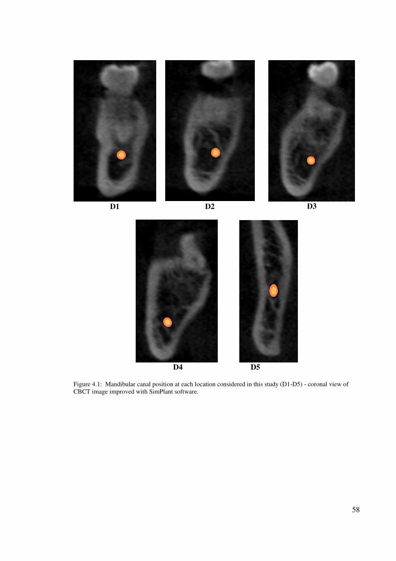
58
D1
D2
D3
D4 D5
Figure 4.1: Mandibular canal position at each location considered in this study (D1-D5) - coronal view of
CBCT image improved with SimPlant software.
59
4.2 Comparison of D locations on the right and left sides
In this study there were 60 patients’ records. The right and left were measured and analyzed
for each location from D1 till D5. The measurement unit used was millimeters in all length
values of this study. The interest was in determining a significant mean difference between
the right and left side of the jaw for each aspect considered in this study along the path of
the mandibular canal.
Table 4.1 summarizes the descriptive statistics for the right and left side of all locations
(D1-D5) which involved mean, SD, Mean of score different, t-statistics, df value and P
value. Four aspects of each location is considered in the statistical test (except D5S) and
their P-values was more than 0.05 so there is no significant difference in the location of the
mandibular canal for the right and left side for the total sample (n=120).
Paired sample t-test was used to compare two population means in the case of the two
samples that are correlated like in ‘before-after’ studies, or when the samples are the
matched pairs or the case is a control study. All the data was assessed to check if it was
normally distributed or not (using the histogram).
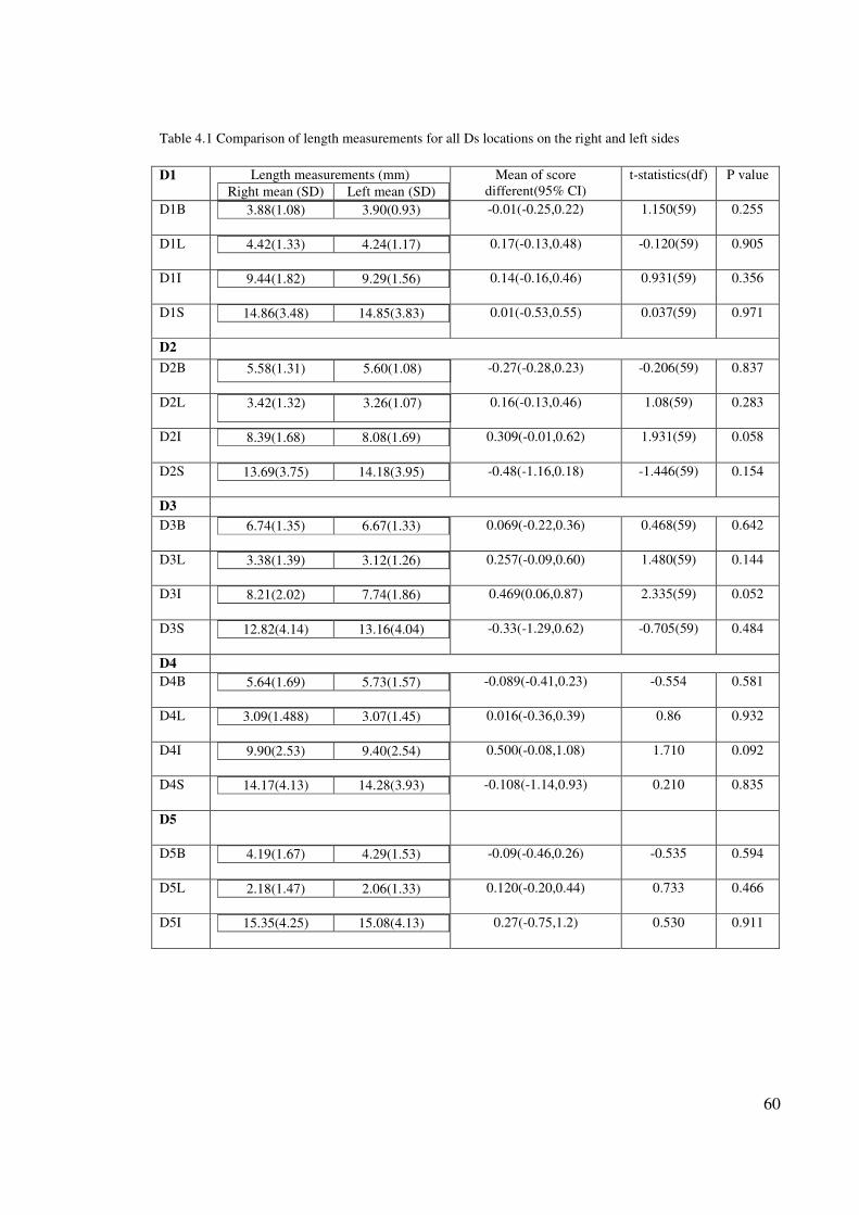
60
Table 4.1 Comparison of length measurements for all Ds locations on the right and left sides
D1 Length measurements (mm)
Right mean (SD) Left mean (SD)
Mean of score
different(95% CI)
t-statistics(df) P value
D1B 3.88(1.08) 3.90(0.93)
-0.01(-0.25,0.22) 1.150(59) 0.255
D1L 4.42(1.33) 4.24(1.17)
0.17(-0.13,0.48) -0.120(59) 0.905
D1I 9.44(1.82) 9.29(1.56)
0.14(-0.16,0.46) 0.931(59) 0.356
D1S 14.86(3.48) 14.85(3.83)
0.01(-0.53,0.55) 0.037(59) 0.971
D2
D2B 5.58(1.31) 5.60(1.08)
-0.27(-0.28,0.23) -0.206(59) 0.837
D2L 3.42(1.32) 3.26(1.07)
0.16(-0.13,0.46) 1.08(59) 0.283
D2I 8.39(1.68) 8.08(1.69)
0.309(-0.01,0.62) 1.931(59) 0.058
D2S 13.69(3.75) 14.18(3.95)
-0.48(-1.16,0.18) -1.446(59) 0.154
D3
D3B 6.74(1.35) 6.67(1.33)
0.069(-0.22,0.36) 0.468(59) 0.642
D3L 3.38(1.39) 3.12(1.26)
0.257(-0.09,0.60) 1.480(59) 0.144
D3I 8.21(2.02) 7.74(1.86)
0.469(0.06,0.87) 2.335(59) 0.052
D3S 12.82(4.14) 13.16(4.04)
-0.33(-1.29,0.62) -0.705(59) 0.484
D4
D4B 5.64(1.69) 5.73(1.57)
-0.089(-0.41,0.23) -0.554 0.581
D4L 3.09(1.488) 3.07(1.45)
0.016(-0.36,0.39) 0.86 0.932
D4I 9.90(2.53) 9.40(2.54)
0.500(-0.08,1.08) 1.710 0.092
D4S 14.17(4.13) 14.28(3.93)
-0.108(-1.14,0.93) 0.210 0.835
D5
D5B 4.19(1.67) 4.29(1.53)
-0.09(-0.46,0.26) -0.535 0.594
D5L 2.18(1.47) 2.06(1.33)
0.120(-0.20,0.44) 0.733 0.466
D5I 15.35(4.25) 15.08(4.13)
0.27(-0.75,1.2) 0.530 0.911
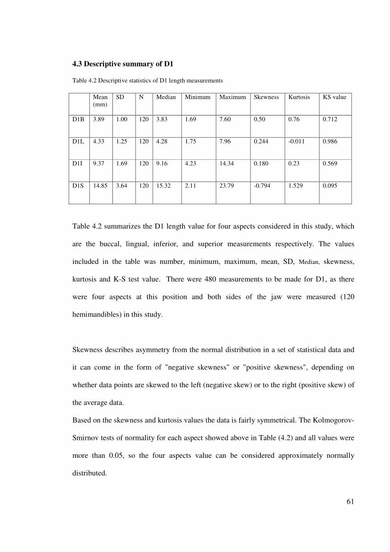
61
4.3 Descriptive summary of D1
Table 4.2 Descriptive statistics of D1 length measurements
Mean
(mm)
SD N Median Minimum Maximum Skewness Kurtosis KS value
D1B 3.89 1.00 120 3.83 1.69 7.60 0.50 0.76 0.712
D1L 4.33 1.25 120 4.28 1.75 7.96 0.244 -0.011 0.986
D1I 9.37 1.69 120 9.16 4.23 14.34 0.180 0.23 0.569
D1S 14.85 3.64 120 15.32 2.11 23.79 -0.794 1.529 0.095
Table 4.2 summarizes the D1 length value for four aspects considered in this study, which
are the buccal, lingual, inferior, and superior measurements respectively. The values
included in the table was number, minimum, maximum, mean, SD, Median, skewness,
kurtosis and K-S test value. There were 480 measurements to be made for D1, as there
were four aspects at this position and both sides of the jaw were measured (120
hemimandibles) in this study.
Skewness describes asymmetry from the normal distribution in a set of statistical data and
it can come in the form of "negative skewness" or "positive skewness", depending on
whether data points are skewed to the left (negative skew) or to the right (positive skew) of
the average data.
Based on the skewness and kurtosis values the data is fairly symmetrical. The Kolmogorov-
Smirnov tests of normality for each aspect showed above in Table (4.2) and all values were
more than 0.05, so the four aspects value can be considered approximately normally
distributed.
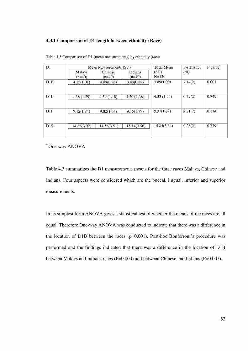
62
4.3.1 Comparison of D1 length between ethnicity (Race)
Table 4.3 Comparison of D1 (mean measurements) by ethnicity (race)
D1
Mean Measurements (SD)
Malays
(n=40)
Chinese
(n=40)
Indians
(n=40)
Total Mean
(SD)
N=120
F-statistics
(df)
P value*
D1B 4.15(1.01) 4.09(0.96) 3.43(0.88)
3.89(1.00) 7.14(2) 0.001
D1L 4.38 (1.29) 4.39 (1.10) 4.20 (1.38)
4.33 (1.25) 0.29(2) 0.749
D1I 9.12(1.84) 9.82(1.34) 9.15(1.79)
9.37(1.69) 2.21(2) 0.114
D1S 14.86(3.92) 14.56(3.51) 15.14(3.56)
14.85(3.64) 0.25(2) 0.779
* One-way ANOVA
Table 4.3 summarizes the D1 measurements means for the three races Malays, Chinese and
Indians. Four aspects were considered which are the buccal, lingual, inferior and superior
measurements.
In its simplest form ANOVA gives a statistical test of whether the means of the races are all
equal. Therefore One-way ANOVA was conducted to indicate that there was a difference in
the location of D1B between the races (p=0.001). Post-hoc Bonferroni’s procedure was
performed and the findings indicated that there was a difference in the location of D1B
between Malays and Indians races (P=0.003) and between Chinese and Indians (P=0.007).
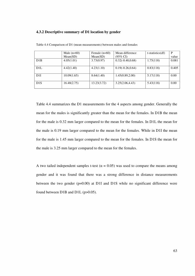
63
4.3.2 Descriptive summary of D1 location by gender
Table 4.4 Comparison of D1 (mean measurements) between males and females
Male (n=60)
Mean(SD)
Female (n=60)
Mean(SD)
Mean difference
(95% CI)
t-statistics(df) P
value
D1B 4.05(1.01) 3.73(0.97) 0.32(-0.40,0.68) 1.75(118) 0.081
D1L 4.42(1.40) 4.23(1.10) 0.19(-0.26,0.64) 0.83(118) 0.405
D1I 10.09(1.65) 8.64(1.40) 1.45(0.89,2.00) 5.17(118) 0.00
D1S 16.48(2.75) 13.23(3.72) 3.25(2.06,4.43) 5.43(118) 0.00
Table 4.4 summarizes the D1 measurements for the 4 aspects among gender. Generally the
mean for the males is significantly greater than the mean for the females. In D1B the mean
for the male is 0.32 mm larger compared to the mean for the females. In D1L the mean for
the male is 0.19 mm larger compared to the mean for the females. While in D1I the mean
for the male is 1.45 mm larger compared to the mean for the females. In D1S the mean for
the male is 3.25 mm larger compared to the mean for the females.
A two tailed independent samples t-test (α = 0.05) was used to compare the means among
gender and it was found that there was a strong difference in distance measurements
between the two gender (p=0.00) at D1I and D1S while no significant difference were
found between D1B and D1L (p>0.05).
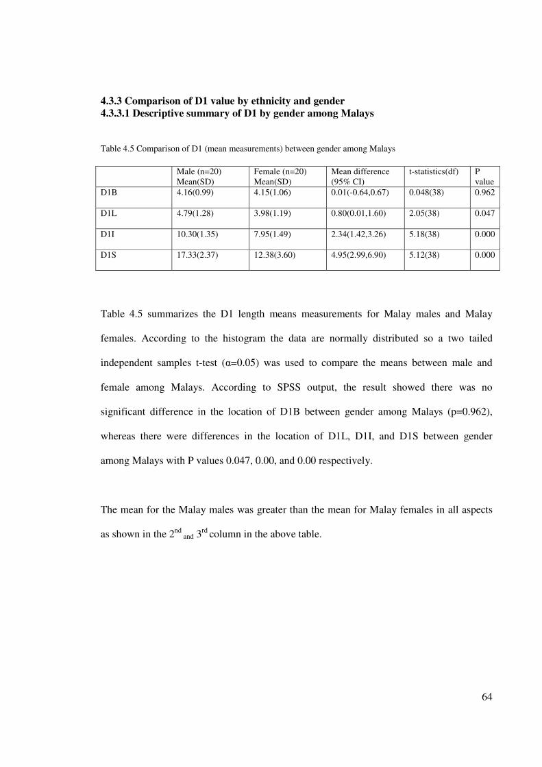
64
4.3.3 Comparison of D1 value by ethnicity and gender
4.3.3.1 Descriptive summary of D1 by gender among Malays
Table 4.5 Comparison of D1 (mean measurements) between gender among Malays
Male (n=20)
Mean(SD)
Female (n=20)
Mean(SD)
Mean difference
(95% CI)
t-statistics(df) P
value
D1B 4.16(0.99) 4.15(1.06) 0.01(-0.64,0.67) 0.048(38) 0.962
D1L 4.79(1.28) 3.98(1.19) 0.80(0.01,1.60) 2.05(38) 0.047
D1I 10.30(1.35) 7.95(1.49) 2.34(1.42,3.26) 5.18(38) 0.000
D1S 17.33(2.37) 12.38(3.60) 4.95(2.99,6.90) 5.12(38) 0.000
Table 4.5 summarizes the D1 length means measurements for Malay males and Malay
females. According to the histogram the data are normally distributed so a two tailed
independent samples t-test (α=0.05) was used to compare the means between male and
female among Malays. According to SPSS output, the result showed there was no
significant difference in the location of D1B between gender among Malays (p=0.962),
whereas there were differences in the location of D1L, D1I, and D1S between gender
among Malays with P values 0.047, 0.00, and 0.00 respectively.
The mean for the Malay males was greater than the mean for Malay females in all aspects
as shown in the 2nd and 3
rd column in the above table.
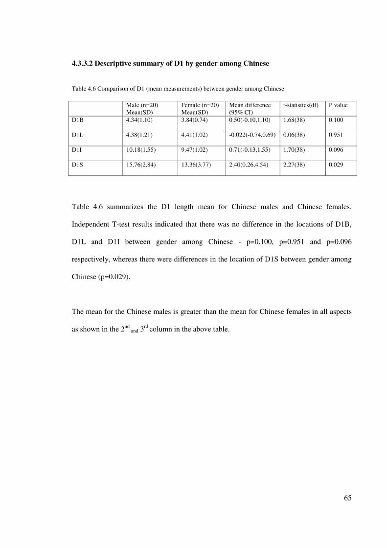
65
4.3.3.2 Descriptive summary of D1 by gender among Chinese
Table 4.6 Comparison of D1 (mean measurements) between gender among Chinese
Male (n=20)
Mean(SD)
Female (n=20)
Mean(SD)
Mean difference
(95% CI)
t-statistics(df) P value
D1B 4.34(1.10) 3.84(0.74) 0.50(-0.10,1.10) 1.68(38) 0.100
D1L 4.38(1.21) 4.41(1.02) -0.022(-0.74,0.69) 0.06(38) 0.951
D1I 10.18(1.55) 9.47(1.02) 0.71(-0.13,1.55) 1.70(38) 0.096
D1S 15.76(2.84) 13.36(3.77) 2.40(0.26,4.54) 2.27(38) 0.029
Table 4.6 summarizes the D1 length mean for Chinese males and Chinese females.
Independent T-test results indicated that there was no difference in the locations of D1B,
D1L and D1I between gender among Chinese - p=0.100, p=0.951 and p=0.096
respectively, whereas there were differences in the location of D1S between gender among
Chinese (p=0.029).
The mean for the Chinese males is greater than the mean for Chinese females in all aspects
as shown in the 2nd
and 3rd
column in the above table.
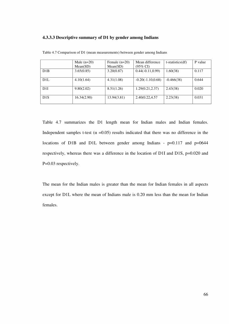
66
4.3.3.3 Descriptive summary of D1 by gender among Indians
Table 4.7 Comparison of D1 (mean measurements) between gender among Indians
Male (n=20)
Mean(SD)
Female (n=20)
Mean(SD)
Mean difference
(95% CI)
t-statistics(df) P value
D1B 3.65(0.85) 3.20(0.87) 0.44(-0.11,0.99) 1.60(38) 0.117
D1L 4.10(1.64) 4.31(1.08) -0.20(-1.10,0.68) -0.466(38) 0.644
D1I 9.80(2.02) 8.51(1.26) 1.29(0.21,2.37) 2.43(38) 0.020
D1S 16.34(2.90) 13.94(3.81) 2.40(0.22,4.57 2.23(38) 0.031
Table 4.7 summarizes the D1 length mean for Indian males and Indian females.
Independent samples t-test (α =0.05) results indicated that there was no difference in the
locations of D1B and D1L between gender among Indians - p=0.117 and p=0644
respectively, whereas there was a difference in the location of D1I and D1S, p=0.020 and
P=0.03 respectively.
The mean for the Indian males is greater than the mean for Indian females in all aspects
except for D1L where the mean of Indians male is 0.20 mm less than the mean for Indian
females.
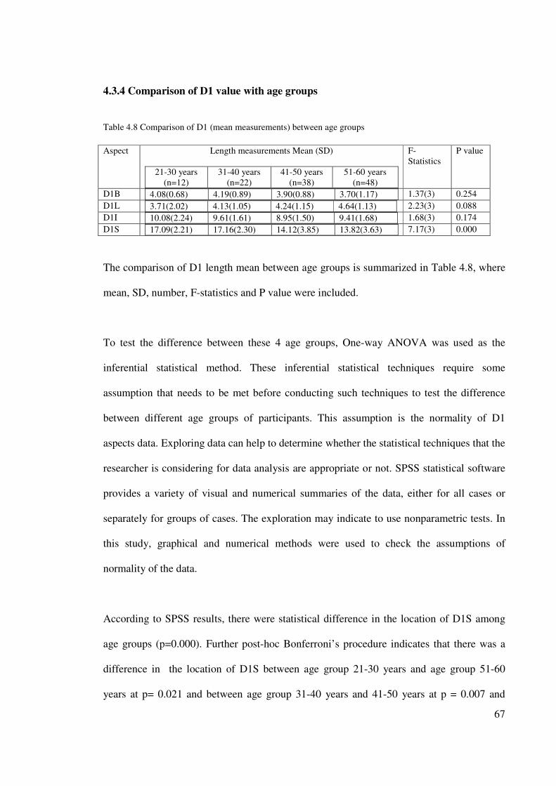
67
4.3.4 Comparison of D1 value with age groups
Table 4.8 Comparison of D1 (mean measurements) between age groups
Aspect Length measurements Mean (SD)
21-30 years
(n=12)
31-40 years
(n=22)
41-50 years
(n=38)
51-60 years
(n=48)
F-
Statistics
P value
D1B 4.08(0.68) 4.19(0.89) 3.90(0.88) 3.70(1.17)
1.37(3) 0.254
D1L 3.71(2.02) 4.13(1.05) 4.24(1.15) 4.64(1.13)
2.23(3) 0.088
D1I 10.08(2.24) 9.61(1.61) 8.95(1.50) 9.41(1.68)
1.68(3) 0.174
D1S 17.09(2.21) 17.16(2.30) 14.12(3.85) 13.82(3.63)
7.17(3) 0.000
The comparison of D1 length mean between age groups is summarized in Table 4.8, where
mean, SD, number, F-statistics and P value were included.
To test the difference between these 4 age groups, One-way ANOVA was used as the
inferential statistical method. These inferential statistical techniques require some
assumption that needs to be met before conducting such techniques to test the difference
between different age groups of participants. This assumption is the normality of D1
aspects data. Exploring data can help to determine whether the statistical techniques that the
researcher is considering for data analysis are appropriate or not. SPSS statistical software
provides a variety of visual and numerical summaries of the data, either for all cases or
separately for groups of cases. The exploration may indicate to use nonparametric tests. In
this study, graphical and numerical methods were used to check the assumptions of
normality of the data.
According to SPSS results, there were statistical difference in the location of D1S among
age groups (p=0.000). Further post-hoc Bonferroni’s procedure indicates that there was a
difference in the location of D1S between age group 21-30 years and age group 51-60
years at p= 0.021 and between age group 31-40 years and 41-50 years at p = 0.007 and
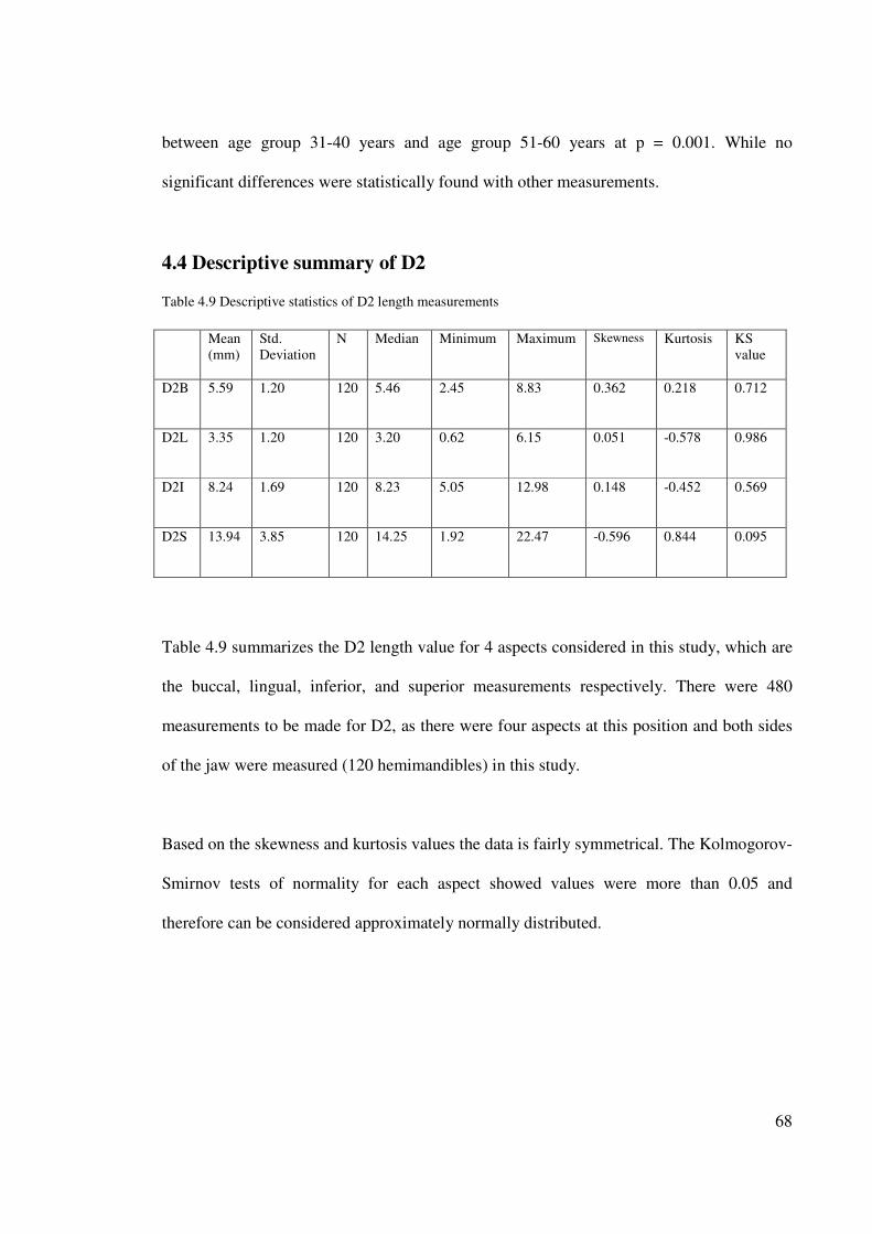
68
between age group 31-40 years and age group 51-60 years at p = 0.001. While no
significant differences were statistically found with other measurements.
4.4 Descriptive summary of D2 Table 4.9 Descriptive statistics of D2 length measurements
Mean
(mm)
Std.
Deviation
N Median Minimum Maximum Skewness Kurtosis KS
value
D2B 5.59 1.20 120 5.46 2.45 8.83 0.362 0.218 0.712
D2L 3.35 1.20 120 3.20 0.62 6.15 0.051 -0.578 0.986
D2I 8.24 1.69 120 8.23 5.05 12.98 0.148 -0.452 0.569
D2S 13.94 3.85 120 14.25 1.92 22.47 -0.596 0.844 0.095
Table 4.9 summarizes the D2 length value for 4 aspects considered in this study, which are
the buccal, lingual, inferior, and superior measurements respectively. There were 480
measurements to be made for D2, as there were four aspects at this position and both sides
of the jaw were measured (120 hemimandibles) in this study.
Based on the skewness and kurtosis values the data is fairly symmetrical. The Kolmogorov-
Smirnov tests of normality for each aspect showed values were more than 0.05 and
therefore can be considered approximately normally distributed.
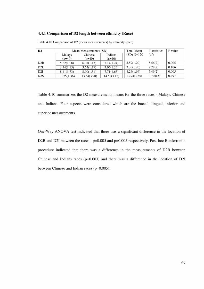
69
4.4.1 Comparison of D2 length between ethnicity (Race)
Table 4.10 Comparison of D2 (mean measurements) by ethnicity (race)
D2
Mean Measurements (SD)
Malays
(n=40)
Chinese
(n=40)
Indians
(n=40)
Total Mean
(SD) N=120
F-statistics
(df)
P value
D2B 5.62(1.08) 6.01(1.13) 5.14(1.24)
5.59(1.20) 5.56(2) 0.005
D2L 3.34(1.13) 3.63(1.17) 3.06(1.25)
3.35(1.20) 2.28(2) 0.106
D2I 8.11(1.73) 8.90(1.51) 7.71(1.63)
8.24(1.69) 5.46(2) 0.005
D2S 13.75(4.36) 13.54(3.98) 14.52(3.12)
13.94(3.85) 0.704(2) 0.497
Table 4.10 summarizes the D2 measurements means for the three races - Malays, Chinese
and Indians. Four aspects were considered which are the buccal, lingual, inferior and
superior measurements.
One-Way ANOVA test indicated that there was a significant difference in the location of
D2B and D2I between the races - p=0.005 and p=0.005 respectively. Post-hoc Bonferroni’s
procedure indicated that there was a difference in the measurements of D2B between
Chinese and Indians races (p=0.003) and there was a difference in the location of D2I
between Chinese and Indian races (p=0.005).
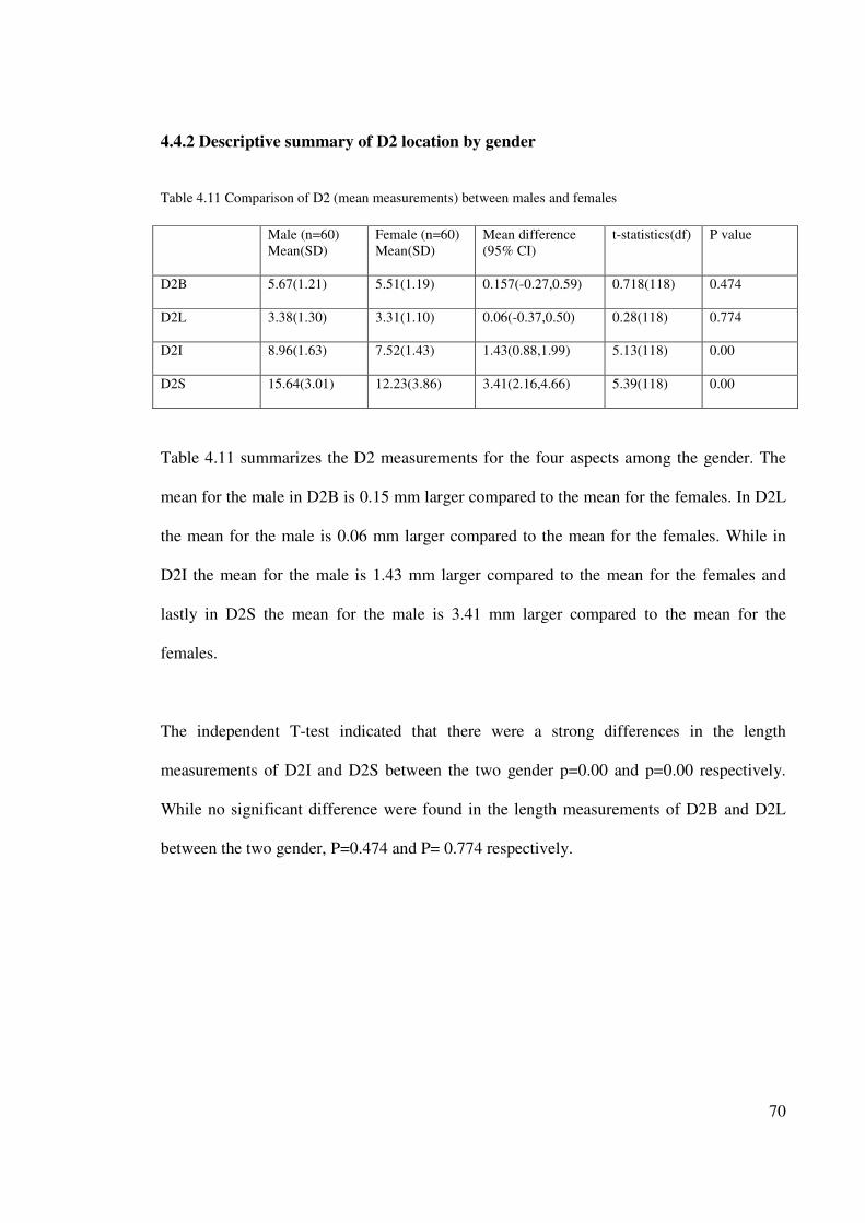
70
4.4.2 Descriptive summary of D2 location by gender
Table 4.11 Comparison of D2 (mean measurements) between males and females
Male (n=60)
Mean(SD)
Female (n=60)
Mean(SD)
Mean difference
(95% CI)
t-statistics(df) P value
D2B 5.67(1.21) 5.51(1.19) 0.157(-0.27,0.59) 0.718(118) 0.474
D2L 3.38(1.30) 3.31(1.10) 0.06(-0.37,0.50) 0.28(118) 0.774
D2I 8.96(1.63) 7.52(1.43) 1.43(0.88,1.99) 5.13(118) 0.00
D2S 15.64(3.01) 12.23(3.86) 3.41(2.16,4.66) 5.39(118) 0.00
Table 4.11 summarizes the D2 measurements for the four aspects among the gender. The
mean for the male in D2B is 0.15 mm larger compared to the mean for the females. In D2L
the mean for the male is 0.06 mm larger compared to the mean for the females. While in
D2I the mean for the male is 1.43 mm larger compared to the mean for the females and
lastly in D2S the mean for the male is 3.41 mm larger compared to the mean for the
females.
The independent T-test indicated that there were a strong differences in the length
measurements of D2I and D2S between the two gender p=0.00 and p=0.00 respectively.
While no significant difference were found in the length measurements of D2B and D2L
between the two gender, P=0.474 and P= 0.774 respectively.
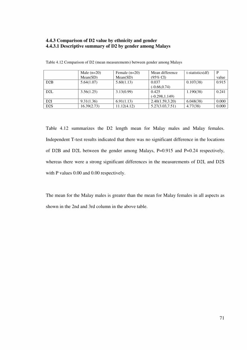
71
4.4.3 Comparison of D2 value by ethnicity and gender
4.4.3.1 Descriptive summary of D2 by gender among Malays
Table 4.12 Comparison of D2 (mean measurements) between gender among Malays
Male (n=20)
Mean(SD)
Female (n=20)
Mean(SD)
Mean difference
(95% CI)
t-statistics(df) P
value
D2B 5.64(1.07) 5.60(1.13) 0.037
(-0.66,0.74)
0.107(38) 0.915
D2L 3.56(1.25) 3.13(0.99) 0.425
(-0.298,1.149)
1.190(38) 0.241
D2I 9.31(1.36) 6.91(1.13) 2.40(1.59,3.20) 6.048(38) 0.000
D2S 16.39(2.73) 11.12(4.12) 5.27(3.03,7.51) 4.77(38) 0.000
Table 4.12 summarizes the D2 length mean for Malay males and Malay females.
Independent T-test results indicated that there was no significant difference in the locations
of D2B and D2L between the gender among Malays, P=0.915 and P=0.24 respectively,
whereas there were a strong significant differences in the measurements of D2I, and D2S
with P values 0.00 and 0.00 respectively.
The mean for the Malay males is greater than the mean for Malay females in all aspects as
shown in the 2nd and 3rd column in the above table.
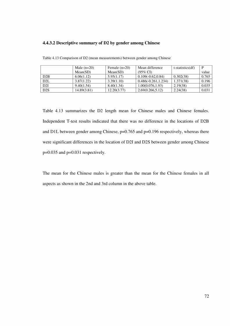
72
4.4.3.2 Descriptive summary of D2 by gender among Chinese
Table 4.13 Comparison of D2 (mean measurements) between gender among Chinese
Male (n=20)
Mean(SD)
Female (n=20)
Mean(SD)
Mean difference
(95% CI)
t-statistics(df) P
value
D2B 6.06(1.12) 5.95(1.17) 0.109(-0.62,0.84) 0.302(38) 0.765
D2L 3.87(1.22) 3.39(1.10) 0.486(-0.261,1.234) 1.371(38) 0.196
D2I 9.40(1.54) 8.40(1.34) 1.00(0.076,1.93) 2.19(38) 0.035
D2S 14.89(3.81) 12.20(3.77) 2.69(0.266,5.12) 2.24(38) 0.031
Table 4.13 summarizes the D2 length mean for Chinese males and Chinese females.
Independent T-test results indicated that there was no difference in the locations of D2B
and D1L between gender among Chinese, p=0.765 and p=0.196 respectively, whereas there
were significant differences in the location of D2I and D2S between gender among Chinese
p=0.035 and p=0.031 respectively.
The mean for the Chinese males is greater than the mean for the Chinese females in all
aspects as shown in the 2nd and 3rd column in the above table.
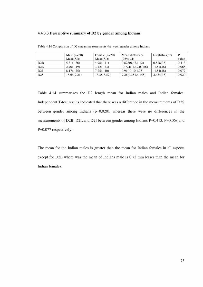
73
4.4.3.3 Descriptive summary of D2 by gender among Indians
Table 4.14 Comparison of D2 (mean measurements) between gender among Indians
Male (n=20)
Mean(SD)
Female (n=20)
Mean(SD)
Mean difference
(95% CI)
t-statistics(df) P
value
D2B 5.31(1.36) 4.98(1.11) 0.828(0.47,1.12) 0.828(38) 0.413
D2L 2.70(1.19) 3.42(1.23) -0.721(-1.49,0.056) -1.87(38) 0.068
D2I 8.17(1.75) 7.25(1.40) 0.91(-0.10,1.93) -1.81(38) 0.077
D2S 15.65(2.21) 13.38(3.52) 2.26(0.381,4.148) 2.434(38) 0.020
Table 4.14 summarizes the D2 length mean for Indian males and Indian females.
Independent T-test results indicated that there was a difference in the measurements of D2S
between gender among Indians (p=0.020), whereas there were no differences in the
measurements of D2B, D2L and D2I between gender among Indians P=0.413, P=0.068 and
P=0.077 respectively.
The mean for the Indian males is greater than the mean for Indian females in all aspects
except for D2L where was the mean of Indians male is 0.72 mm lesser than the mean for
Indian females.
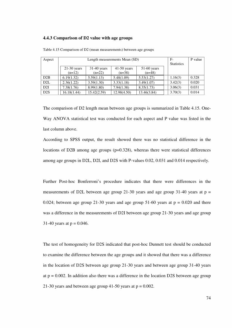
74
4.4.3 Comparison of D2 value with age groups
Table 4.15 Comparison of D2 (mean measurements) between age groups
Aspect Length measurements Mean (SD)
21-30 years
(n=12)
31-40 years
(n=22)
41-50 years
(n=38)
51-60 years
(n=48)
F-
Statistics
P value
D2B 6.19(1.32) 5.59(1.13) 5.48(1.09) 5.53(1.27)
1.16(3) 0.328
D2L 2.36(1.22) 3.59(1.30) 3.33(1.18) 3.49(1.07)
3.42(3) 0.020
D2I 7.38(1.76) 8.99(1.80) 7.94(1.38) 8.35(1.73)
3.06(3) 0.031
D2S 16.18(1.44) 15.42(2.59) 12.98(4.50) 13.46(3.84)
3.70(3) 0.014
The comparison of D2 length mean between age groups is summarized in Table 4.15. One-
Way ANOVA statistical test was conducted for each aspect and P value was listed in the
last column above.
According to SPSS output, the result showed there was no statistical difference in the
locations of D2B among age groups (p=0.328), whereas there were statistical differences
among age groups in D2L, D2I, and D2S with P-values 0.02, 0.031 and 0.014 respectively.
Further Post-hoc Bonferroni’s procedure indicates that there were differences in the
measurements of D2L between age group 21-30 years and age group 31-40 years at p =
0.024; between age group 21-30 years and age group 51-60 years at p = 0.020 and there
was a difference in the measurements of D2I between age group 21-30 years and age group
31-40 years at p = 0.046.
The test of homogeneity for D2S indicated that post-hoc Dunnett test should be conducted
to examine the difference between the age groups and it showed that there was a difference
in the location of D2S between age group 21-30 years and between age group 31-40 years
at p = 0.002. In addition also there was a difference in the location D2S between age group
21-30 years and between age group 41-50 years at p = 0.002.
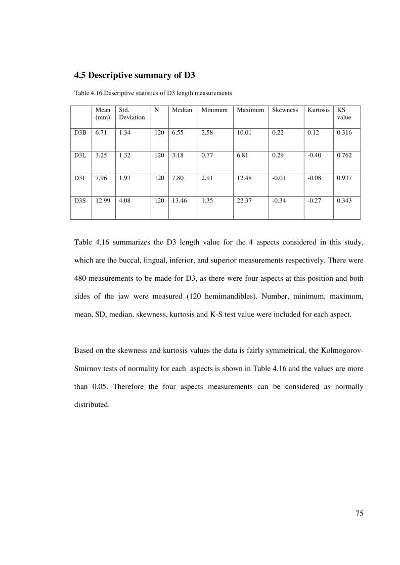
75
4.5 Descriptive summary of D3 Table 4.16 Descriptive statistics of D3 length measurements
Mean
(mm)
Std.
Deviation
N Median Minimum Maximum Skewness Kurtosis KS
value
D3B 6.71 1.34 120 6.55 2.58 10.01 0.22 0.12 0.316
D3L 3.25 1.32 120 3.18 0.77 6.81 0.29 -0.40 0.762
D3I 7.96 1.93 120 7.80 2.91 12.48 -0.01 -0.08 0.937
D3S 12.99 4.08 120 13.46 1.35 22.37 -0.34 -0.27 0.343
Table 4.16 summarizes the D3 length value for the 4 aspects considered in this study,
which are the buccal, lingual, inferior, and superior measurements respectively. There were
480 measurements to be made for D3, as there were four aspects at this position and both
sides of the jaw were measured (120 hemimandibles). Number, minimum, maximum,
mean, SD, median, skewness, kurtosis and K-S test value were included for each aspect.
Based on the skewness and kurtosis values the data is fairly symmetrical, the Kolmogorov-
Smirnov tests of normality for each aspects is shown in Table 4.16 and the values are more
than 0.05. Therefore the four aspects measurements can be considered as normally
distributed.
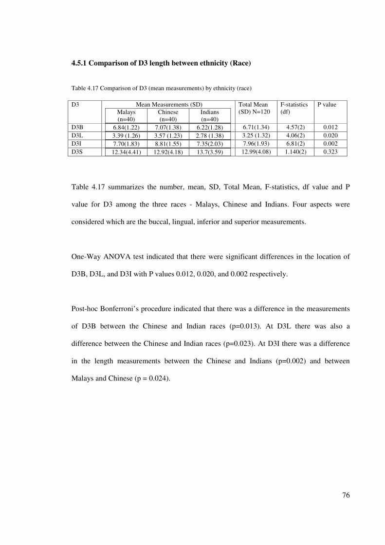
76
4.5.1 Comparison of D3 length between ethnicity (Race)
Table 4.17 Comparison of D3 (mean measurements) by ethnicity (race)
D3
Mean Measurements (SD)
Malays
(n=40)
Chinese
(n=40)
Indians
(n=40)
Total Mean
(SD) N=120
F-statistics
(df)
P value
D3B 6.84(1.22) 7.07(1.38) 6.22(1.28)
6.71(1.34) 4.57(2) 0.012
D3L 3.39 (1.26) 3.57 (1.23) 2.78 (1.38)
3.25 (1.32) 4.06(2) 0.020
D3I 7.70(1.83) 8.81(1.55) 7.35(2.03)
7.96(1.93) 6.81(2) 0.002
D3S 12.34(4.41) 12.92(4.18) 13.7(3.59)
12.99(4.08) 1.140(2) 0.323
Table 4.17 summarizes the number, mean, SD, Total Mean, F-statistics, df value and P
value for D3 among the three races - Malays, Chinese and Indians. Four aspects were
considered which are the buccal, lingual, inferior and superior measurements.
One-Way ANOVA test indicated that there were significant differences in the location of
D3B, D3L, and D3I with P values 0.012, 0.020, and 0.002 respectively.
Post-hoc Bonferroni’s procedure indicated that there was a difference in the measurements
of D3B between the Chinese and Indian races (p=0.013). At D3L there was also a
difference between the Chinese and Indian races (p=0.023). At D3I there was a difference
in the length measurements between the Chinese and Indians (p=0.002) and between
Malays and Chinese (p = 0.024).
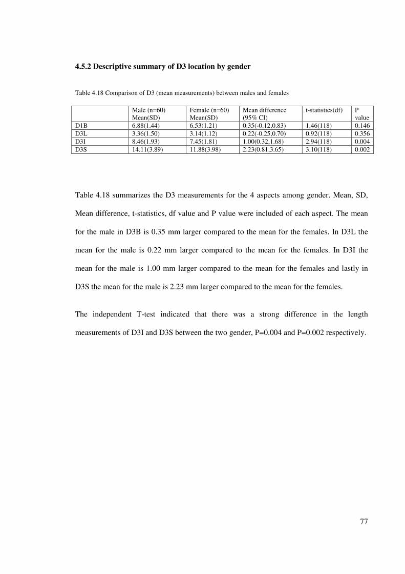
77
4.5.2 Descriptive summary of D3 location by gender
Table 4.18 Comparison of D3 (mean measurements) between males and females
Male (n=60)
Mean(SD)
Female (n=60)
Mean(SD)
Mean difference
(95% CI)
t-statistics(df) P
value
D1B 6.88(1.44) 6.53(1.21) 0.35(-0.12,0.83) 1.46(118) 0.146
D3L 3.36(1.50) 3.14(1.12) 0.22(-0.25,0.70) 0.92(118) 0.356
D3I 8.46(1.93) 7.45(1.81) 1.00(0.32,1.68) 2.94(118) 0.004
D3S 14.11(3.89) 11.88(3.98) 2.23(0.81,3.65) 3.10(118) 0.002
Table 4.18 summarizes the D3 measurements for the 4 aspects among gender. Mean, SD,
Mean difference, t-statistics, df value and P value were included of each aspect. The mean
for the male in D3B is 0.35 mm larger compared to the mean for the females. In D3L the
mean for the male is 0.22 mm larger compared to the mean for the females. In D3I the
mean for the male is 1.00 mm larger compared to the mean for the females and lastly in
D3S the mean for the male is 2.23 mm larger compared to the mean for the females.
The independent T-test indicated that there was a strong difference in the length
measurements of D3I and D3S between the two gender, P=0.004 and P=0.002 respectively.
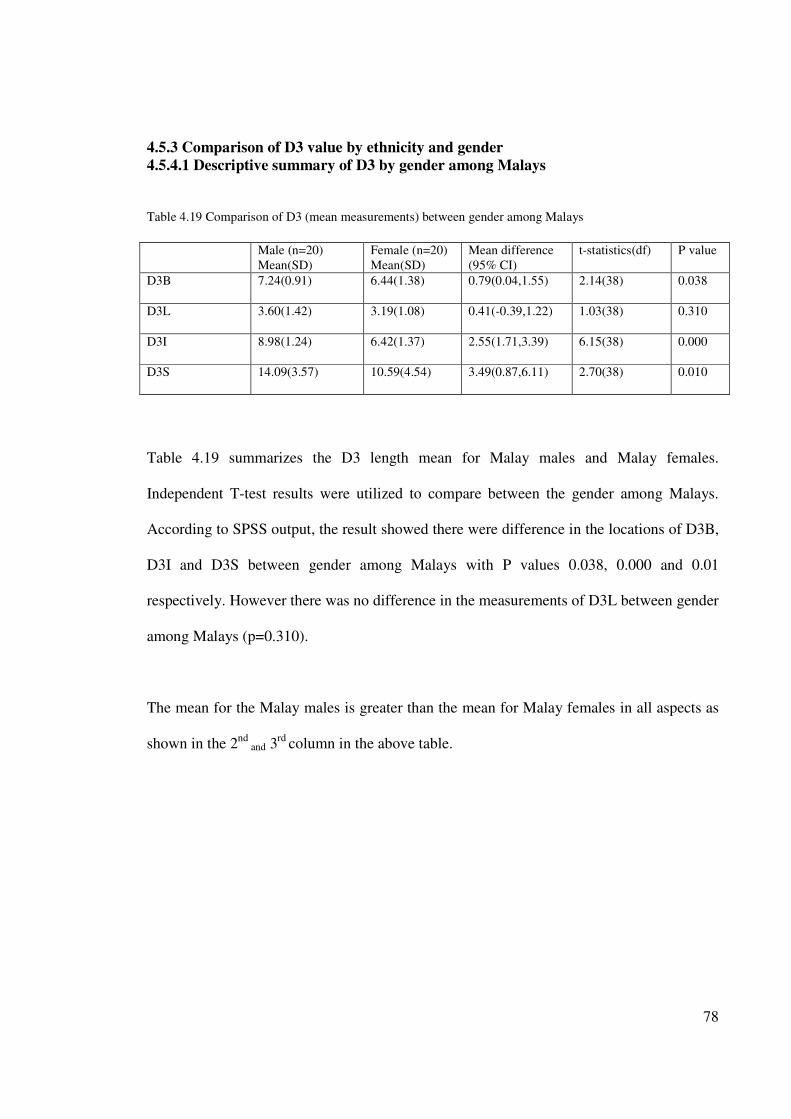
78
4.5.3 Comparison of D3 value by ethnicity and gender
4.5.4.1 Descriptive summary of D3 by gender among Malays
Table 4.19 Comparison of D3 (mean measurements) between gender among Malays
Male (n=20)
Mean(SD)
Female (n=20)
Mean(SD)
Mean difference
(95% CI)
t-statistics(df) P value
D3B 7.24(0.91) 6.44(1.38) 0.79(0.04,1.55) 2.14(38) 0.038
D3L 3.60(1.42) 3.19(1.08) 0.41(-0.39,1.22) 1.03(38) 0.310
D3I 8.98(1.24) 6.42(1.37) 2.55(1.71,3.39) 6.15(38) 0.000
D3S 14.09(3.57) 10.59(4.54) 3.49(0.87,6.11) 2.70(38) 0.010
Table 4.19 summarizes the D3 length mean for Malay males and Malay females.
Independent T-test results were utilized to compare between the gender among Malays.
According to SPSS output, the result showed there were difference in the locations of D3B,
D3I and D3S between gender among Malays with P values 0.038, 0.000 and 0.01
respectively. However there was no difference in the measurements of D3L between gender
among Malays (p=0.310).
The mean for the Malay males is greater than the mean for Malay females in all aspects as
shown in the 2nd
and 3rd
column in the above table.
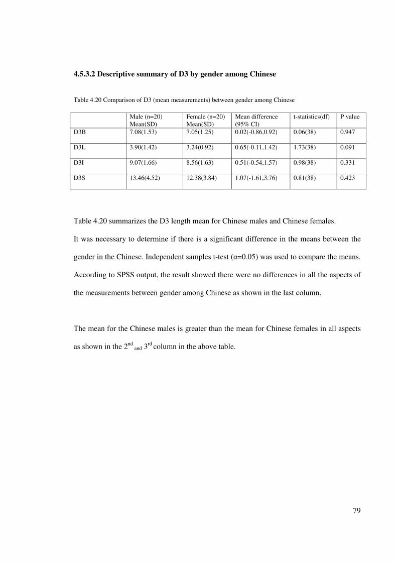
79
4.5.3.2 Descriptive summary of D3 by gender among Chinese
Table 4.20 Comparison of D3 (mean measurements) between gender among Chinese
Male (n=20)
Mean(SD)
Female (n=20)
Mean(SD)
Mean difference
(95% CI)
t-statistics(df) P value
D3B 7.08(1.53) 7.05(1.25) 0.02(-0.86,0.92) 0.06(38) 0.947
D3L 3.90(1.42) 3.24(0.92) 0.65(-0.11,1.42) 1.73(38) 0.091
D3I 9.07(1.66) 8.56(1.63) 0.51(-0.54,1.57) 0.98(38) 0.331
D3S 13.46(4.52) 12.38(3.84) 1.07(-1.61,3.76) 0.81(38) 0.423
Table 4.20 summarizes the D3 length mean for Chinese males and Chinese females.
It was necessary to determine if there is a significant difference in the means between the
gender in the Chinese. Independent samples t-test (α=0.05) was used to compare the means.
According to SPSS output, the result showed there were no differences in all the aspects of
the measurements between gender among Chinese as shown in the last column.
The mean for the Chinese males is greater than the mean for Chinese females in all aspects
as shown in the 2nd
and 3rd
column in the above table.
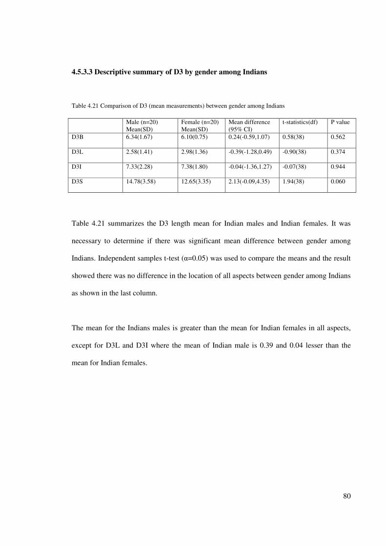
80
4.5.3.3 Descriptive summary of D3 by gender among Indians
Table 4.21 Comparison of D3 (mean measurements) between gender among Indians
Male (n=20)
Mean(SD)
Female (n=20)
Mean(SD)
Mean difference
(95% CI)
t-statistics(df) P value
D3B 6.34(1.67) 6.10(0.75) 0.24(-0.59,1.07) 0.58(38) 0.562
D3L 2.58(1.41) 2.98(1.36) -0.39(-1.28,0.49) -0.90(38) 0.374
D3I 7.33(2.28) 7.38(1.80) -0.04(-1.36,1.27) -0.07(38) 0.944
D3S 14.78(3.58) 12.65(3.35) 2.13(-0.09,4.35) 1.94(38) 0.060
Table 4.21 summarizes the D3 length mean for Indian males and Indian females. It was
necessary to determine if there was significant mean difference between gender among
Indians. Independent samples t-test (α=0.05) was used to compare the means and the result
showed there was no difference in the location of all aspects between gender among Indians
as shown in the last column.
The mean for the Indians males is greater than the mean for Indian females in all aspects,
except for D3L and D3I where the mean of Indian male is 0.39 and 0.04 lesser than the
mean for Indian females.
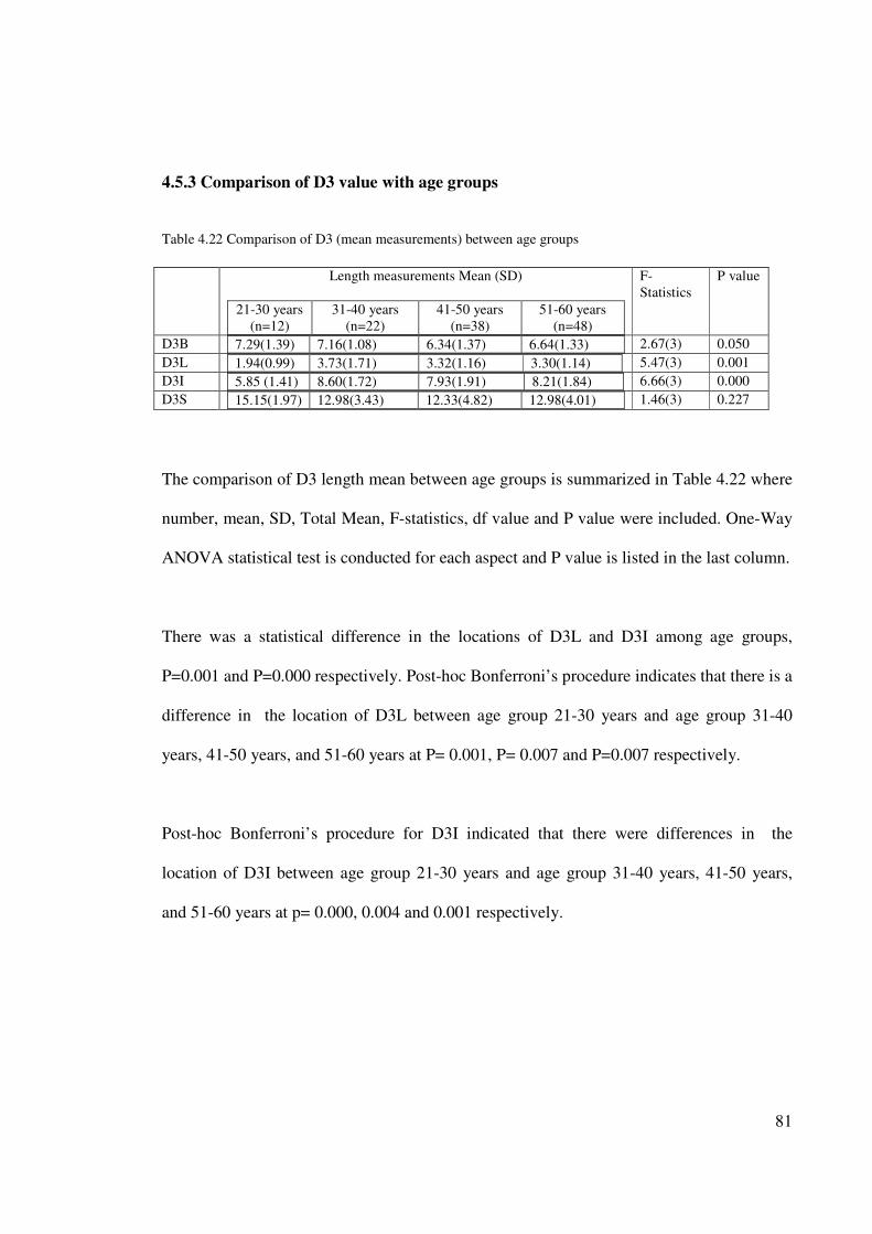
81
4.5.3 Comparison of D3 value with age groups
Table 4.22 Comparison of D3 (mean measurements) between age groups
Length measurements Mean (SD)
21-30 years
(n=12)
31-40 years
(n=22)
41-50 years
(n=38)
51-60 years
(n=48)
F-
Statistics
P value
D3B 7.29(1.39) 7.16(1.08) 6.34(1.37) 6.64(1.33)
2.67(3) 0.050
D3L 1.94(0.99) 3.73(1.71) 3.32(1.16) 3.30(1.14)
5.47(3) 0.001
D3I 5.85 (1.41) 8.60(1.72) 7.93(1.91) 8.21(1.84)
6.66(3) 0.000
D3S 15.15(1.97) 12.98(3.43) 12.33(4.82) 12.98(4.01)
1.46(3) 0.227
The comparison of D3 length mean between age groups is summarized in Table 4.22 where
number, mean, SD, Total Mean, F-statistics, df value and P value were included. One-Way
ANOVA statistical test is conducted for each aspect and P value is listed in the last column.
There was a statistical difference in the locations of D3L and D3I among age groups,
P=0.001 and P=0.000 respectively. Post-hoc Bonferroni’s procedure indicates that there is a
difference in the location of D3L between age group 21-30 years and age group 31-40
years, 41-50 years, and 51-60 years at P= 0.001, P= 0.007 and P=0.007 respectively.
Post-hoc Bonferroni’s procedure for D3I indicated that there were differences in the
location of D3I between age group 21-30 years and age group 31-40 years, 41-50 years,
and 51-60 years at p= 0.000, 0.004 and 0.001 respectively.
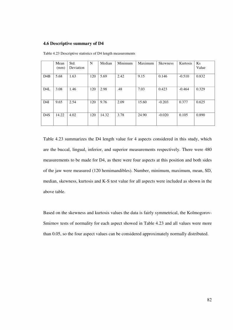
82
4.6 Descriptive summary of D4
Table 4.23 Descriptive statistics of D4 length measurements
Mean
(mm)
Std.
Deviation
N Median Minimum Maximum Skewness Kurtosis Ks
Value
D4B 5.68 1.63 120 5.69 2.42 9.15 0.146 -0.510 0.832
D4L 3.08 1.46 120 2.98 .48 7.03 0.423 -0.464 0.329
D4I 9.65 2.54 120 9.76 2.09 15.60 -0.203 0.377 0.625
D4S 14.22 4.02 120 14.32 3.78 24.90 -0.020 0.105 0.890
Table 4.23 summarizes the D4 length value for 4 aspects considered in this study, which
are the buccal, lingual, inferior, and superior measurements respectively. There were 480
measurements to be made for D4, as there were four aspects at this position and both sides
of the jaw were measured (120 hemimandibles). Number, minimum, maximum, mean, SD,
median, skewness, kurtosis and K-S test value for all aspects were included as shown in the
above table.
Based on the skewness and kurtosis values the data is fairly symmetrical, the Kolmogorov-
Smirnov tests of normality for each aspect showed in Table 4.23 and all values were more
than 0.05, so the four aspect values can be considered approximately normally distributed.
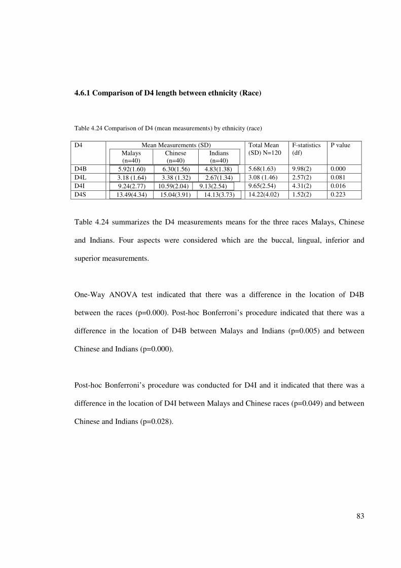
83
4.6.1 Comparison of D4 length between ethnicity (Race)
Table 4.24 Comparison of D4 (mean measurements) by ethnicity (race)
D4
Mean Measurements (SD)
Malays
(n=40)
Chinese
(n=40)
Indians
(n=40)
Total Mean
(SD) N=120
F-statistics
(df)
P value
D4B 5.92(1.60) 6.30(1.56) 4.83(1.38)
5.68(1.63) 9.98(2) 0.000
D4L 3.18 (1.64) 3.38 (1.32) 2.67(1.34)
3.08 (1.46) 2.57(2) 0.081
D4I 9.24(2.77) 10.59(2.04) 9.13(2.54)
9.65(2.54) 4.31(2) 0.016
D4S 13.49(4.34) 15.04(3.91) 14.13(3.73)
14.22(4.02) 1.52(2) 0.223
Table 4.24 summarizes the D4 measurements means for the three races Malays, Chinese
and Indians. Four aspects were considered which are the buccal, lingual, inferior and
superior measurements.
One-Way ANOVA test indicated that there was a difference in the location of D4B
between the races (p=0.000). Post-hoc Bonferroni’s procedure indicated that there was a
difference in the location of D4B between Malays and Indians (p=0.005) and between
Chinese and Indians (p=0.000).
Post-hoc Bonferroni’s procedure was conducted for D4I and it indicated that there was a
difference in the location of D4I between Malays and Chinese races (p=0.049) and between
Chinese and Indians (p=0.028).
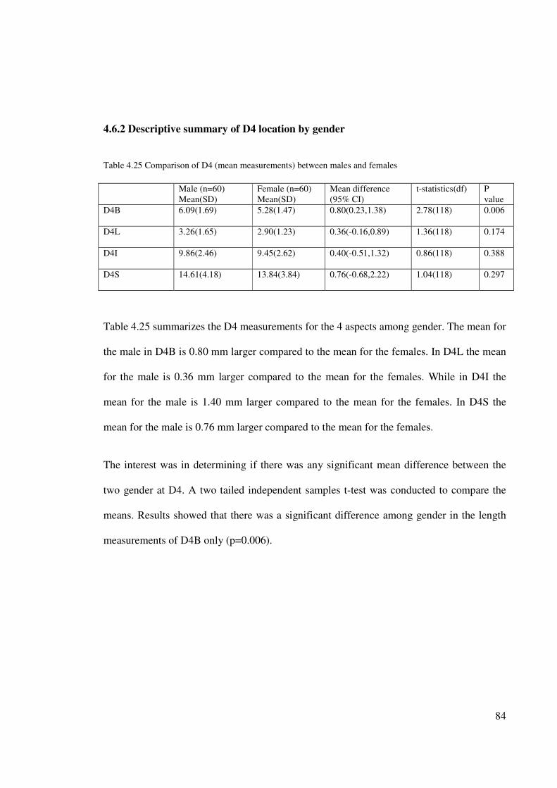
84
4.6.2 Descriptive summary of D4 location by gender
Table 4.25 Comparison of D4 (mean measurements) between males and females
Male (n=60)
Mean(SD)
Female (n=60)
Mean(SD)
Mean difference
(95% CI)
t-statistics(df) P
value
D4B 6.09(1.69) 5.28(1.47) 0.80(0.23,1.38) 2.78(118) 0.006
D4L 3.26(1.65) 2.90(1.23) 0.36(-0.16,0.89) 1.36(118) 0.174
D4I 9.86(2.46) 9.45(2.62) 0.40(-0.51,1.32) 0.86(118) 0.388
D4S 14.61(4.18) 13.84(3.84) 0.76(-0.68,2.22) 1.04(118) 0.297
Table 4.25 summarizes the D4 measurements for the 4 aspects among gender. The mean for
the male in D4B is 0.80 mm larger compared to the mean for the females. In D4L the mean
for the male is 0.36 mm larger compared to the mean for the females. While in D4I the
mean for the male is 1.40 mm larger compared to the mean for the females. In D4S the
mean for the male is 0.76 mm larger compared to the mean for the females.
The interest was in determining if there was any significant mean difference between the
two gender at D4. A two tailed independent samples t-test was conducted to compare the
means. Results showed that there was a significant difference among gender in the length
measurements of D4B only (p=0.006).
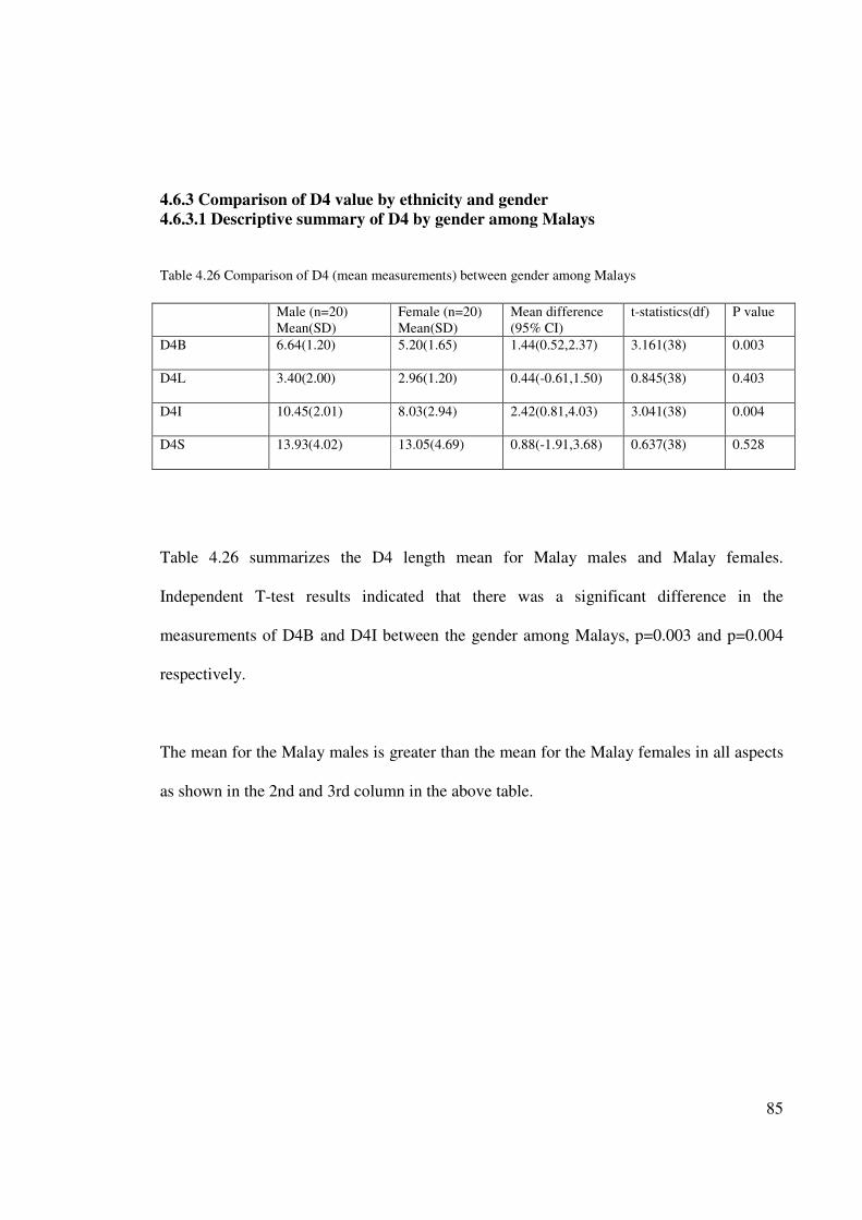
85
4.6.3 Comparison of D4 value by ethnicity and gender
4.6.3.1 Descriptive summary of D4 by gender among Malays
Table 4.26 Comparison of D4 (mean measurements) between gender among Malays
Male (n=20)
Mean(SD)
Female (n=20)
Mean(SD)
Mean difference
(95% CI)
t-statistics(df) P value
D4B 6.64(1.20) 5.20(1.65) 1.44(0.52,2.37) 3.161(38) 0.003
D4L 3.40(2.00) 2.96(1.20) 0.44(-0.61,1.50) 0.845(38) 0.403
D4I 10.45(2.01) 8.03(2.94) 2.42(0.81,4.03) 3.041(38) 0.004
D4S 13.93(4.02) 13.05(4.69) 0.88(-1.91,3.68) 0.637(38) 0.528
Table 4.26 summarizes the D4 length mean for Malay males and Malay females.
Independent T-test results indicated that there was a significant difference in the
measurements of D4B and D4I between the gender among Malays, p=0.003 and p=0.004
respectively.
The mean for the Malay males is greater than the mean for the Malay females in all aspects
as shown in the 2nd and 3rd column in the above table.
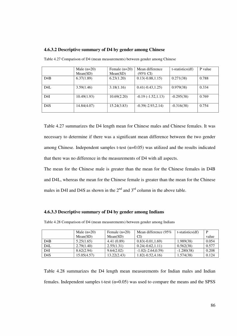
86
4.6.3.2 Descriptive summary of D4 by gender among Chinese
Table 4.27 Comparison of D4 (mean measurements) between gender among Chinese
Male (n=20)
Mean(SD)
Female (n=20)
Mean(SD)
Mean difference
(95% CI)
t-statistics(df) P value
D4B 6.37(1.89) 6.23(1.20) 0.13(-0.88,1.15) 0.271(38) 0.788
D4L 3.59(1.46) 3.18(1.16) 0.41(-0.43,1.25) 0.979(38) 0.334
D4I 10.49(1.93) 10.69(2.20) -0.19 (-1.52,1.13) -0.295(38) 0.769
D4S 14.84(4.07) 15.24(3.83) -0.39(-2.93,2.14) -0.316(38) 0.754
Table 4.27 summarizes the D4 length mean for Chinese males and Chinese females. It was
necessary to determine if there was a significant mean difference between the two gender
among Chinese. Independent samples t-test (α=0.05) was utilized and the results indicated
that there was no difference in the measurements of D4 with all aspects.
The mean for the Chinese male is greater than the mean for the Chinese females in D4B
and D4L, whereas the mean for the Chinese female is greater than the mean for the Chinese
males in D4I and D4S as shown in the 2nd and 3rd column in the above table.
4.6.3.3 Descriptive summary of D4 by gender among Indians
Table 4.28 Comparison of D4 (mean measurements) between gender among Indians
Male (n=20)
Mean(SD)
Female (n=20)
Mean(SD)
Mean difference (95%
CI)
t-statistics(df) P
value
D4B 5.25(1.65) 4.41 (0.89) 0.83(-0.01,1.69) 1.989(38) 0.054
D4L 2.79(1.40) 2.55(1.31) 0.24(-0.62,1.11) 0.562(38) 0.577
D4I 8.62(2.94) 9.64(2.02) -1.02(-2.64,0.59) -1.280(38) 0.208
D4S 15.05(4.57) 13.22(2.43) 1.82(-0.52,4.16) 1.574(38) 0.124
Table 4.28 summarizes the D4 length mean measurements for Indian males and Indian
females. Independent samples t-test (α=0.05) was used to compare the means and the SPSS
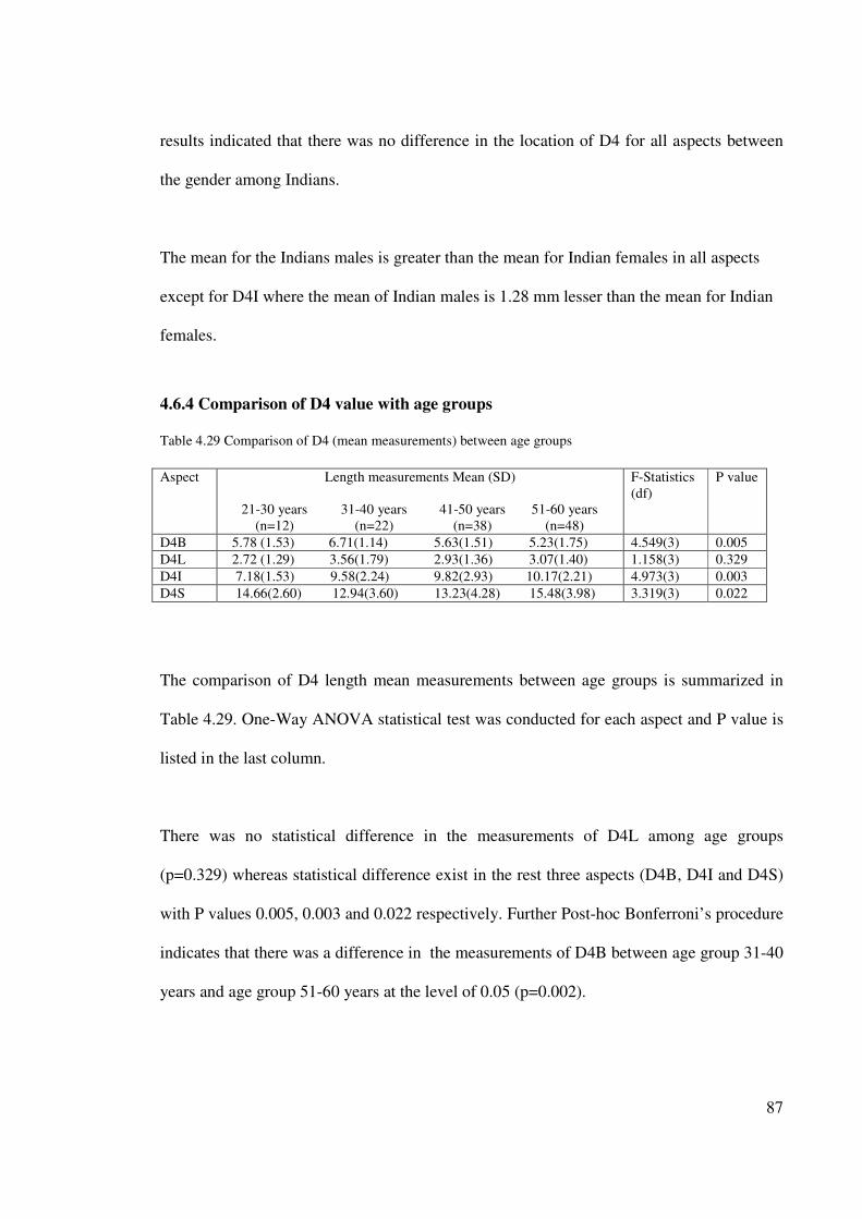
87
results indicated that there was no difference in the location of D4 for all aspects between
the gender among Indians.
The mean for the Indians males is greater than the mean for Indian females in all aspects
except for D4I where the mean of Indian males is 1.28 mm lesser than the mean for Indian
females.
4.6.4 Comparison of D4 value with age groups
Table 4.29 Comparison of D4 (mean measurements) between age groups
Aspect Length measurements Mean (SD)
21-30 years
(n=12)
31-40 years
(n=22)
41-50 years
(n=38)
51-60 years
(n=48)
F-Statistics
(df)
P value
D4B 5.78 (1.53) 6.71(1.14) 5.63(1.51) 5.23(1.75)
4.549(3) 0.005
D4L 2.72 (1.29) 3.56(1.79) 2.93(1.36) 3.07(1.40)
1.158(3) 0.329
D4I 7.18(1.53) 9.58(2.24) 9.82(2.93) 10.17(2.21)
4.973(3) 0.003
D4S 14.66(2.60) 12.94(3.60) 13.23(4.28) 15.48(3.98)
3.319(3) 0.022
The comparison of D4 length mean measurements between age groups is summarized in
Table 4.29. One-Way ANOVA statistical test was conducted for each aspect and P value is
listed in the last column.
There was no statistical difference in the measurements of D4L among age groups
(p=0.329) whereas statistical difference exist in the rest three aspects (D4B, D4I and D4S)
with P values 0.005, 0.003 and 0.022 respectively. Further Post-hoc Bonferroni’s procedure
indicates that there was a difference in the measurements of D4B between age group 31-40
years and age group 51-60 years at the level of 0.05 (p=0.002).
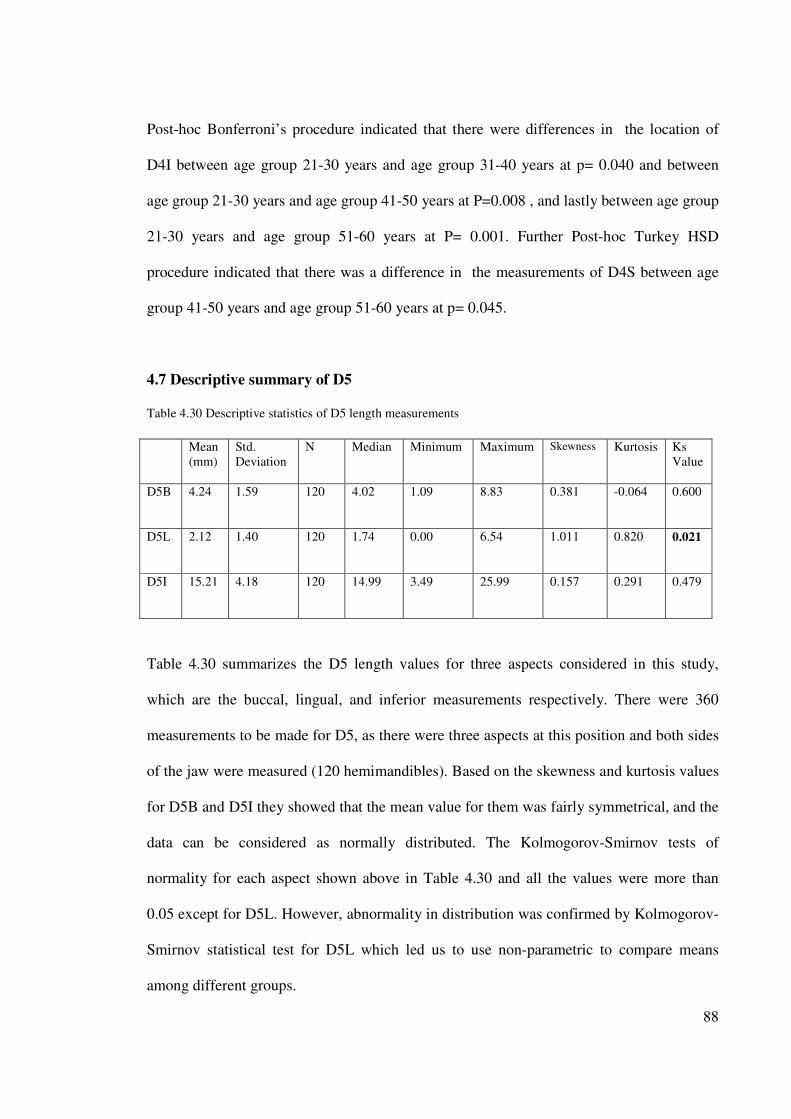
88
Post-hoc Bonferroni’s procedure indicated that there were differences in the location of
D4I between age group 21-30 years and age group 31-40 years at p= 0.040 and between
age group 21-30 years and age group 41-50 years at P=0.008 , and lastly between age group
21-30 years and age group 51-60 years at P= 0.001. Further Post-hoc Turkey HSD
procedure indicated that there was a difference in the measurements of D4S between age
group 41-50 years and age group 51-60 years at p= 0.045.
4.7 Descriptive summary of D5
Table 4.30 Descriptive statistics of D5 length measurements
Mean
(mm)
Std.
Deviation
N Median Minimum Maximum Skewness Kurtosis Ks
Value
D5B 4.24 1.59 120 4.02 1.09 8.83 0.381 -0.064 0.600
D5L 2.12 1.40 120 1.74 0.00 6.54 1.011 0.820 0.021
D5I 15.21 4.18 120 14.99 3.49 25.99 0.157 0.291 0.479
Table 4.30 summarizes the D5 length values for three aspects considered in this study,
which are the buccal, lingual, and inferior measurements respectively. There were 360
measurements to be made for D5, as there were three aspects at this position and both sides
of the jaw were measured (120 hemimandibles). Based on the skewness and kurtosis values
for D5B and D5I they showed that the mean value for them was fairly symmetrical, and the
data can be considered as normally distributed. The Kolmogorov-Smirnov tests of
normality for each aspect shown above in Table 4.30 and all the values were more than
0.05 except for D5L. However, abnormality in distribution was confirmed by Kolmogorov-
Smirnov statistical test for D5L which led us to use non-parametric to compare means
among different groups.
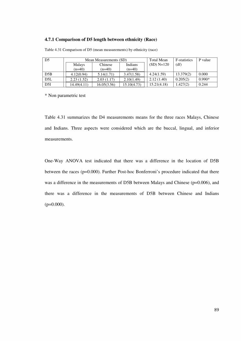
89
4.7.1 Comparison of D5 length between ethnicity (Race)
Table 4.31 Comparison of D5 (mean measurements) by ethnicity (race)
D5
Mean Measurements (SD)
Malays
(n=40)
Chinese
(n=40)
Indians
(n=40)
Total Mean
(SD) N=120
F-statistics
(df)
P value
D5B 4.12(0.94) 5.14(1.71) 3.47(1.58)
4.24(1.59) 13.379(2) 0.000
D5L 2.23 (1.52) 2.03 (1.17) 2.10(1.49)
2.12 (1.40) 0.205(2) 0.990*
D5I 14.49(4.11) 16.05(3.56) 15.10(4.73)
15.21(4.18) 1.427(2) 0.244
* Non parametric test
Table 4.31 summarizes the D4 measurements means for the three races Malays, Chinese
and Indians. Three aspects were considered which are the buccal, lingual, and inferior
measurements.
One-Way ANOVA test indicated that there was a difference in the location of D5B
between the races (p=0.000). Further Post-hoc Bonferroni’s procedure indicated that there
was a difference in the measurements of D5B between Malays and Chinese (p=0.006), and
there was a difference in the measurements of D5B between Chinese and Indians
(p=0.000).
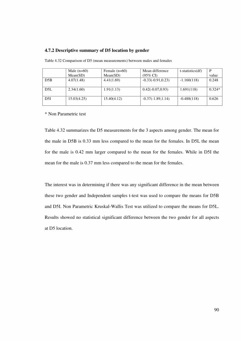
90
4.7.2 Descriptive summary of D5 location by gender
Table 4.32 Comparison of D5 (mean measurements) between males and females
Male (n=60)
Mean(SD)
Female (n=60)
Mean(SD)
Mean difference
(95% CI)
t-statistics(df) P
value
D5B 4.07(1.48) 4.41(1.69) -0.33(-0.91,0.23) -1.160(118) 0.248
D5L 2.34(1.60) 1.91(1.13) 0.42(-0.07,0.93) 1.691(118) 0.324*
D5I 15.03(4.25) 15.40(4.12) -0.37(-1.89,1.14) -0.488(118) 0.626
* Non Parametric test
Table 4.32 summarizes the D5 measurements for the 3 aspects among gender. The mean for
the male in D5B is 0.33 mm less compared to the mean for the females. In D5L the mean
for the male is 0.42 mm larger compared to the mean for the females. While in D5I the
mean for the male is 0.37 mm less compared to the mean for the females.
The interest was in determining if there was any significant difference in the mean between
these two gender and Independent samples t-test was used to compare the means for D5B
and D5I. Non Parametric Kruskal-Wallis Test was utilized to compare the means for D5L.
Results showed no statistical significant difference between the two gender for all aspects
at D5 location.
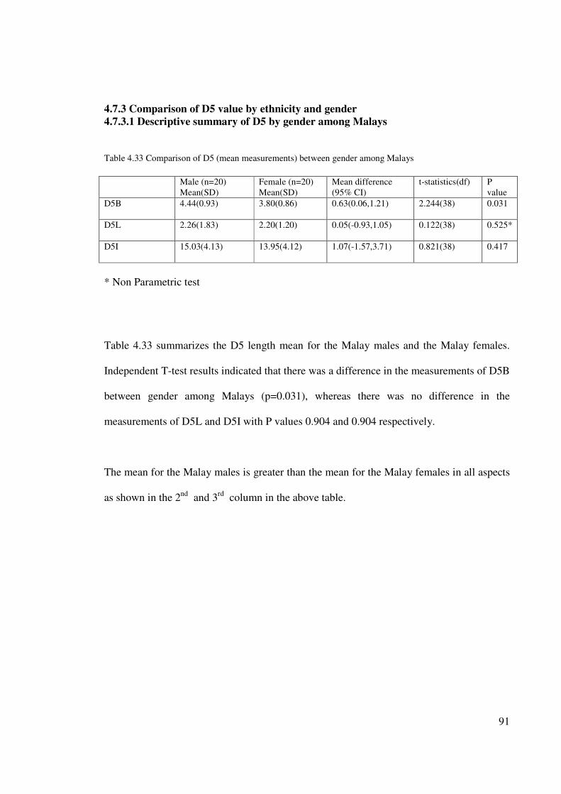
91
4.7.3 Comparison of D5 value by ethnicity and gender
4.7.3.1 Descriptive summary of D5 by gender among Malays
Table 4.33 Comparison of D5 (mean measurements) between gender among Malays
Male (n=20)
Mean(SD)
Female (n=20)
Mean(SD)
Mean difference
(95% CI)
t-statistics(df) P
value
D5B 4.44(0.93) 3.80(0.86) 0.63(0.06,1.21) 2.244(38) 0.031
D5L 2.26(1.83) 2.20(1.20) 0.05(-0.93,1.05) 0.122(38) 0.525*
D5I 15.03(4.13) 13.95(4.12) 1.07(-1.57,3.71) 0.821(38) 0.417
* Non Parametric test
Table 4.33 summarizes the D5 length mean for the Malay males and the Malay females.
Independent T-test results indicated that there was a difference in the measurements of D5B
between gender among Malays (p=0.031), whereas there was no difference in the
measurements of D5L and D5I with P values 0.904 and 0.904 respectively.
The mean for the Malay males is greater than the mean for the Malay females in all aspects
as shown in the 2nd
and 3rd
column in the above table.
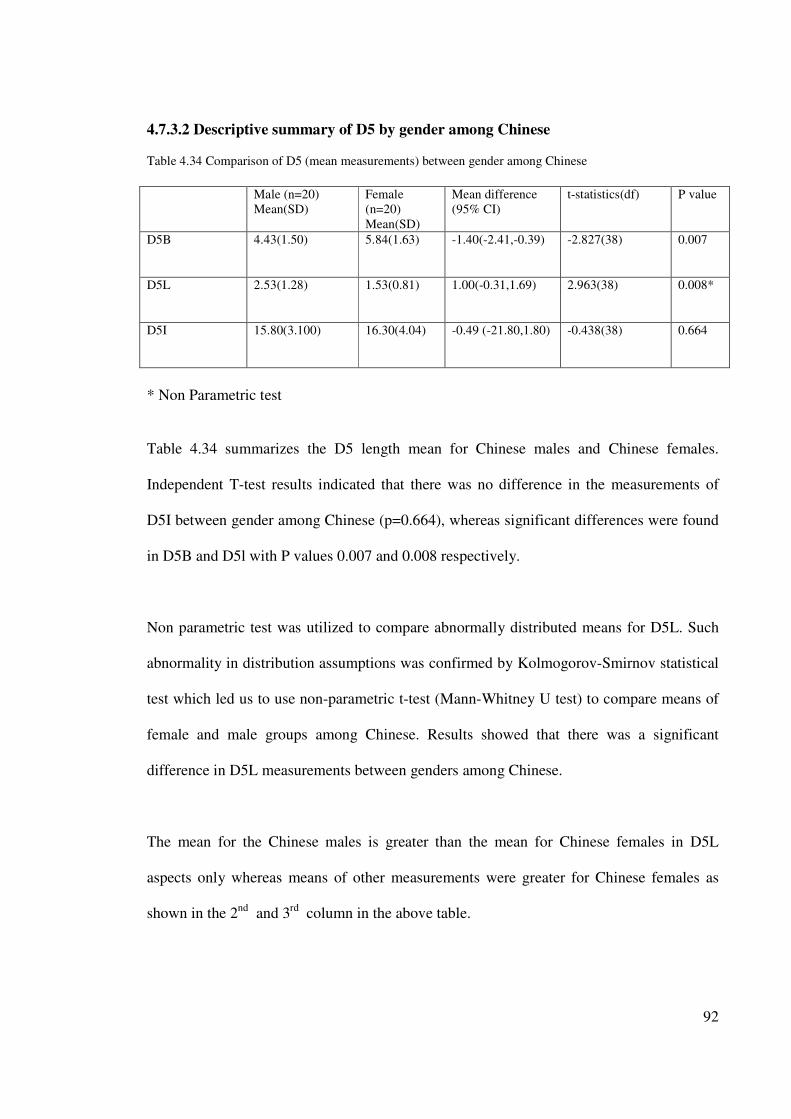
92
4.7.3.2 Descriptive summary of D5 by gender among Chinese
Table 4.34 Comparison of D5 (mean measurements) between gender among Chinese
Male (n=20)
Mean(SD)
Female
(n=20)
Mean(SD)
Mean difference
(95% CI)
t-statistics(df) P value
D5B 4.43(1.50) 5.84(1.63) -1.40(-2.41,-0.39) -2.827(38) 0.007
D5L 2.53(1.28) 1.53(0.81) 1.00(-0.31,1.69) 2.963(38) 0.008*
D5I 15.80(3.100) 16.30(4.04) -0.49 (-21.80,1.80) -0.438(38) 0.664
* Non Parametric test
Table 4.34 summarizes the D5 length mean for Chinese males and Chinese females.
Independent T-test results indicated that there was no difference in the measurements of
D5I between gender among Chinese (p=0.664), whereas significant differences were found
in D5B and D5l with P values 0.007 and 0.008 respectively.
Non parametric test was utilized to compare abnormally distributed means for D5L. Such
abnormality in distribution assumptions was confirmed by Kolmogorov-Smirnov statistical
test which led us to use non-parametric t-test (Mann-Whitney U test) to compare means of
female and male groups among Chinese. Results showed that there was a significant
difference in D5L measurements between genders among Chinese.
The mean for the Chinese males is greater than the mean for Chinese females in D5L
aspects only whereas means of other measurements were greater for Chinese females as
shown in the 2nd and 3rd column in the above table.
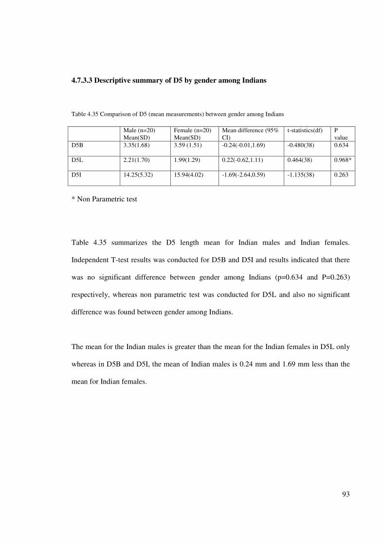
93
4.7.3.3 Descriptive summary of D5 by gender among Indians
Table 4.35 Comparison of D5 (mean measurements) between gender among Indians
Male (n=20)
Mean(SD)
Female (n=20)
Mean(SD)
Mean difference (95%
CI)
t-statistics(df) P
value
D5B 3.35(1.68) 3.59 (1.51) -0.24(-0.01,1.69) -0.480(38) 0.634
D5L 2.21(1.70) 1.99(1.29) 0.22(-0.62,1.11) 0.464(38) 0.968*
D5I 14.25(5.32) 15.94(4.02) -1.69(-2.64,0.59) -1.135(38) 0.263
* Non Parametric test
Table 4.35 summarizes the D5 length mean for Indian males and Indian females.
Independent T-test results was conducted for D5B and D5I and results indicated that there
was no significant difference between gender among Indians (p=0.634 and P=0.263)
respectively, whereas non parametric test was conducted for D5L and also no significant
difference was found between gender among Indians.
The mean for the Indian males is greater than the mean for the Indian females in D5L only
whereas in D5B and D5I, the mean of Indian males is 0.24 mm and 1.69 mm less than the
mean for Indian females.
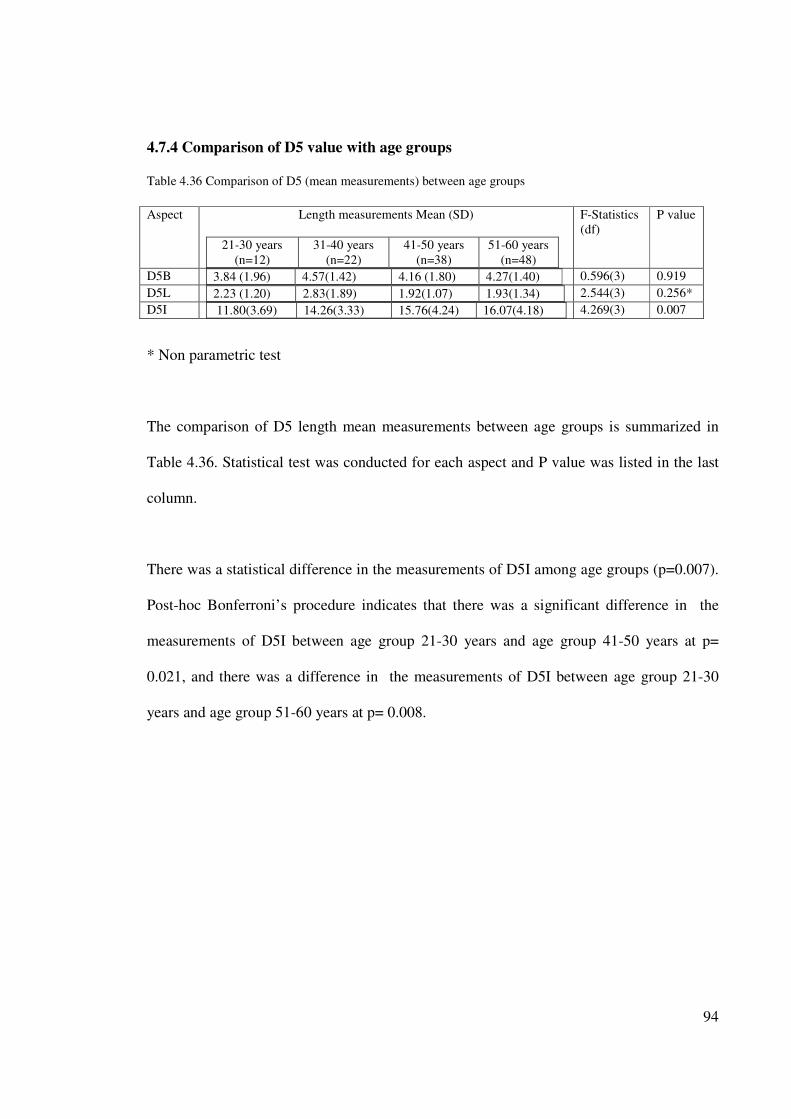
94
4.7.4 Comparison of D5 value with age groups
Table 4.36 Comparison of D5 (mean measurements) between age groups
Aspect Length measurements Mean (SD)
21-30 years
(n=12)
31-40 years
(n=22)
41-50 years
(n=38)
51-60 years
(n=48)
F-Statistics
(df)
P value
D5B 3.84 (1.96) 4.57(1.42) 4.16 (1.80) 4.27(1.40)
0.596(3) 0.919
D5L 2.23 (1.20) 2.83(1.89) 1.92(1.07) 1.93(1.34)
2.544(3) 0.256*
D5I 11.80(3.69) 14.26(3.33) 15.76(4.24) 16.07(4.18)
4.269(3) 0.007
* Non parametric test
The comparison of D5 length mean measurements between age groups is summarized in
Table 4.36. Statistical test was conducted for each aspect and P value was listed in the last
column.
There was a statistical difference in the measurements of D5I among age groups (p=0.007).
Post-hoc Bonferroni’s procedure indicates that there was a significant difference in the
measurements of D5I between age group 21-30 years and age group 41-50 years at p=
0.021, and there was a difference in the measurements of D5I between age group 21-30
years and age group 51-60 years at p= 0.008.
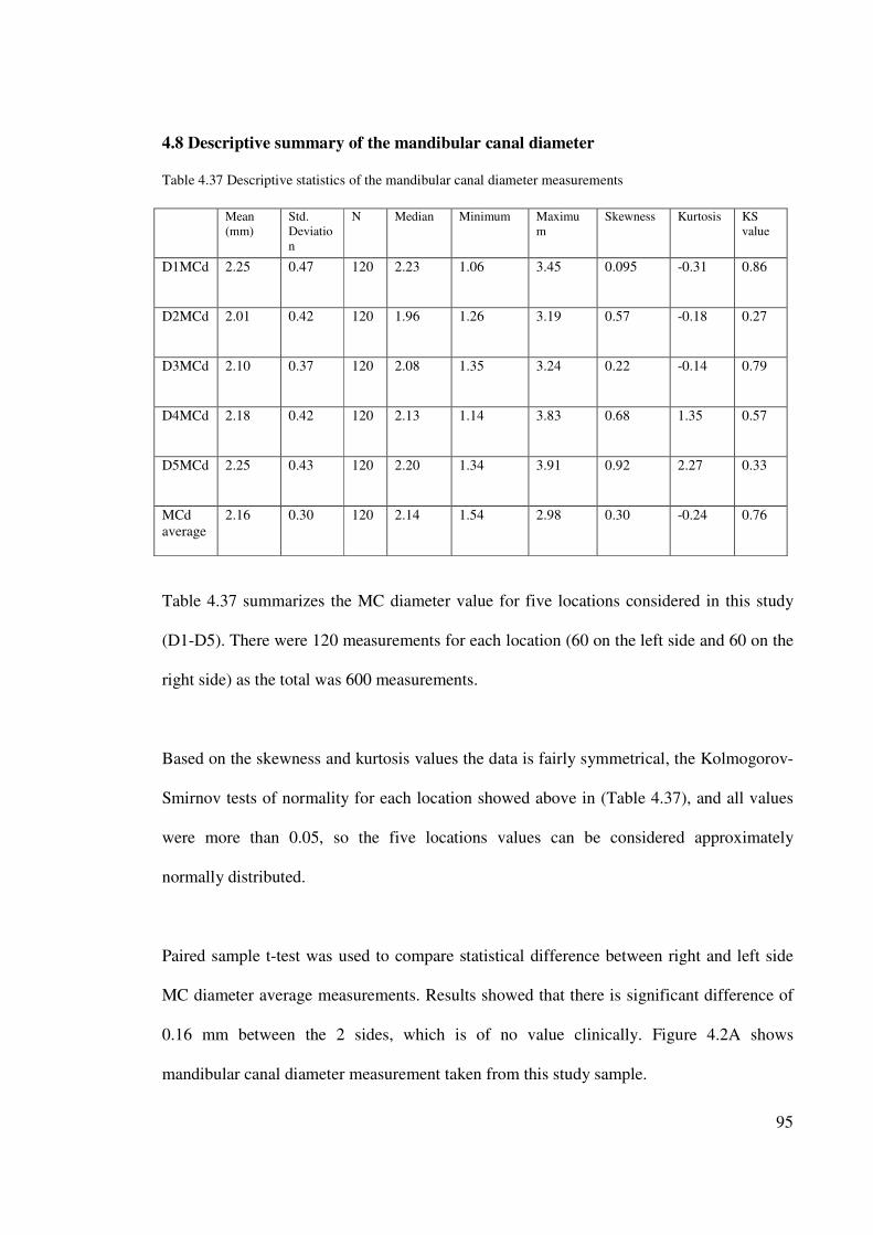
95
4.8 Descriptive summary of the mandibular canal diameter
Table 4.37 Descriptive statistics of the mandibular canal diameter measurements
Mean
(mm)
Std.
Deviatio
n
N Median Minimum Maximu
m
Skewness Kurtosis KS
value
D1MCd 2.25 0.47 120 2.23 1.06 3.45 0.095 -0.31 0.86
D2MCd 2.01 0.42 120 1.96 1.26 3.19 0.57 -0.18 0.27
D3MCd 2.10 0.37 120 2.08 1.35 3.24 0.22 -0.14 0.79
D4MCd 2.18 0.42 120 2.13 1.14 3.83 0.68 1.35 0.57
D5MCd 2.25 0.43 120 2.20 1.34 3.91 0.92 2.27 0.33
MCd
average
2.16 0.30 120 2.14 1.54 2.98 0.30 -0.24 0.76
Table 4.37 summarizes the MC diameter value for five locations considered in this study
(D1-D5). There were 120 measurements for each location (60 on the left side and 60 on the
right side) as the total was 600 measurements.
Based on the skewness and kurtosis values the data is fairly symmetrical, the Kolmogorov-
Smirnov tests of normality for each location showed above in (Table 4.37), and all values
were more than 0.05, so the five locations values can be considered approximately
normally distributed.
Paired sample t-test was used to compare statistical difference between right and left side
MC diameter average measurements. Results showed that there is significant difference of
0.16 mm between the 2 sides, which is of no value clinically. Figure 4.2A shows
mandibular canal diameter measurement taken from this study sample.
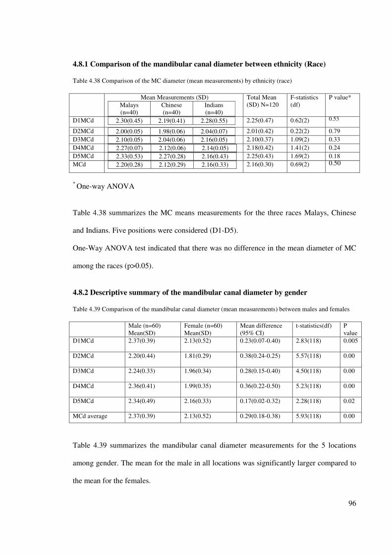
96
4.8.1 Comparison of the mandibular canal diameter between ethnicity (Race)
Table 4.38 Comparison of the MC diameter (mean measurements) by ethnicity (race)
Mean Measurements (SD)
Malays
(n=40)
Chinese
(n=40)
Indians
(n=40)
Total Mean
(SD) N=120
F-statistics
(df)
P value*
D1MCd 2.30(0.45) 2.19(0.41) 2.28(0.55)
2.25(0.47) 0.62(2) 0.53
D2MCd 2.00(0.05) 1.98(0.06) 2.04(0.07)
2.01(0.42) 0.22(2) 0.79
D3MCd 2.10(0.05) 2.04(0.06) 2.16(0.05)
2.10(0.37) 1.09(2) 0.33
D4MCd 2.27(0.07) 2.12(0.06) 2.14(0.05)
2.18(0.42) 1.41(2) 0.24
D5MCd 2.33(0.53) 2.27(0.28) 2.16(0.43)
2.25(0.43) 1.69(2) 0.18
MCd 2.20(0.28) 2.12(0.29) 2.16(0.33)
2.16(0.30) 0.69(2) 0.50
* One-way ANOVA
Table 4.38 summarizes the MC means measurements for the three races Malays, Chinese
and Indians. Five positions were considered (D1-D5).
One-Way ANOVA test indicated that there was no difference in the mean diameter of MC
among the races (p>0.05).
4.8.2 Descriptive summary of the mandibular canal diameter by gender
Table 4.39 Comparison of the mandibular canal diameter (mean measurements) between males and females
Male (n=60)
Mean(SD)
Female (n=60)
Mean(SD)
Mean difference
(95% CI)
t-statistics(df) P
value
D1MCd 2.37(0.39) 2.13(0.52) 0.23(0.07-0.40) 2.83(118) 0.005
D2MCd 2.20(0.44) 1.81(0.29) 0.38(0.24-0.25) 5.57(118) 0.00
D3MCd 2.24(0.33) 1.96(0.34) 0.28(0.15-0.40) 4.50(118) 0.00
D4MCd 2.36(0.41) 1.99(0.35) 0.36(0.22-0.50) 5.23(118) 0.00
D5MCd 2.34(0.49) 2.16(0.33) 0.17(0.02-0.32) 2.28(118) 0.02
MCd average 2.37(0.39) 2.13(0.52) 0.29(0.18-0.38) 5.93(118) 0.00
Table 4.39 summarizes the mandibular canal diameter measurements for the 5 locations
among gender. The mean for the male in all locations was significantly larger compared to
the mean for the females.
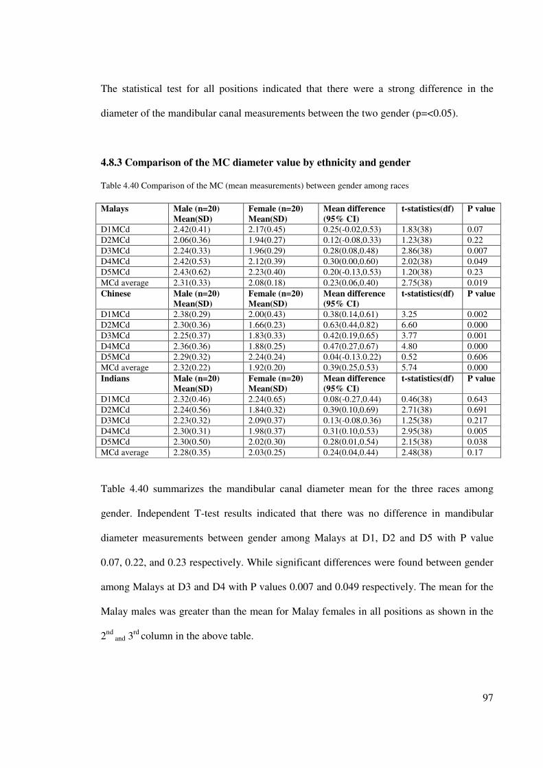
97
The statistical test for all positions indicated that there were a strong difference in the
diameter of the mandibular canal measurements between the two gender (p=<0.05).
4.8.3 Comparison of the MC diameter value by ethnicity and gender
Table 4.40 Comparison of the MC (mean measurements) between gender among races
Malays Male (n=20)
Mean(SD)
Female (n=20)
Mean(SD)
Mean difference
(95% CI)
t-statistics(df) P value
D1MCd 2.42(0.41) 2.17(0.45) 0.25(-0.02,0.53) 1.83(38) 0.07
D2MCd 2.06(0.36) 1.94(0.27) 0.12(-0.08,0.33) 1.23(38) 0.22
D3MCd 2.24(0.33) 1.96(0.29) 0.28(0.08,0.48) 2.86(38) 0.007
D4MCd 2.42(0.53) 2.12(0.39) 0.30(0.00,0.60) 2.02(38) 0.049
D5MCd 2.43(0.62) 2.23(0.40) 0.20(-0.13,0.53) 1.20(38) 0.23
MCd average 2.31(0.33) 2.08(0.18) 0.23(0.06,0.40) 2.75(38) 0.019
Chinese Male (n=20)
Mean(SD)
Female (n=20)
Mean(SD)
Mean difference
(95% CI)
t-statistics(df) P value
D1MCd 2.38(0.29) 2.00(0.43) 0.38(0.14,0.61) 3.25 0.002
D2MCd 2.30(0.36) 1.66(0.23) 0.63(0.44,0.82) 6.60 0.000
D3MCd 2.25(0.37) 1.83(0.33) 0.42(0.19,0.65) 3.77 0.001
D4MCd 2.36(0.36) 1.88(0.25) 0.47(0.27,0.67) 4.80 0.000
D5MCd 2.29(0.32) 2.24(0.24) 0.04(-0.13.0.22) 0.52 0.606
MCd average 2.32(0.22) 1.92(0.20) 0.39(0.25,0.53) 5.74 0.000
Indians Male (n=20)
Mean(SD)
Female (n=20)
Mean(SD)
Mean difference
(95% CI)
t-statistics(df) P value
D1MCd 2.32(0.46) 2.24(0.65) 0.08(-0.27,0.44) 0.46(38) 0.643
D2MCd 2.24(0.56) 1.84(0.32) 0.39(0.10,0.69) 2.71(38) 0.691
D3MCd 2.23(0.32) 2.09(0.37) 0.13(-0.08,0.36) 1.25(38) 0.217
D4MCd 2.30(0.31) 1.98(0.37) 0.31(0.10,0.53) 2.95(38) 0.005
D5MCd 2.30(0.50) 2.02(0.30) 0.28(0.01,0.54) 2.15(38) 0.038
MCd average 2.28(0.35) 2.03(0.25) 0.24(0.04,0.44) 2.48(38) 0.17
Table 4.40 summarizes the mandibular canal diameter mean for the three races among
gender. Independent T-test results indicated that there was no difference in mandibular
diameter measurements between gender among Malays at D1, D2 and D5 with P value
0.07, 0.22, and 0.23 respectively. While significant differences were found between gender
among Malays at D3 and D4 with P values 0.007 and 0.049 respectively. The mean for the
Malay males was greater than the mean for Malay females in all positions as shown in the
2nd
and 3rd
column in the above table.

98
While among Chinese, there was no difference in the diameter of the mandibular canal at
D5MCd between gender (p=0.606), whereas there were strong significant differences in the
MC diameter for the other positions (D1MCd-D4MCd). The MC diameter mean for the
Chinese males is greater than the mean for Chinese females in all positions as shown in the
2nd
and 3rd
column in the above table.
Furthermore, results among Indians showed that there was no difference in the MC
diameter at D1MCd, D2MCd and D3MCd; whereas there were significant differences in
the MC diameter measurements at D4MCd and D5MCd with P values 0.005 and 0.038
respectively. The mandibular canal mean measurements for the Indian males are greater
than the mean for Indian females in all positions.
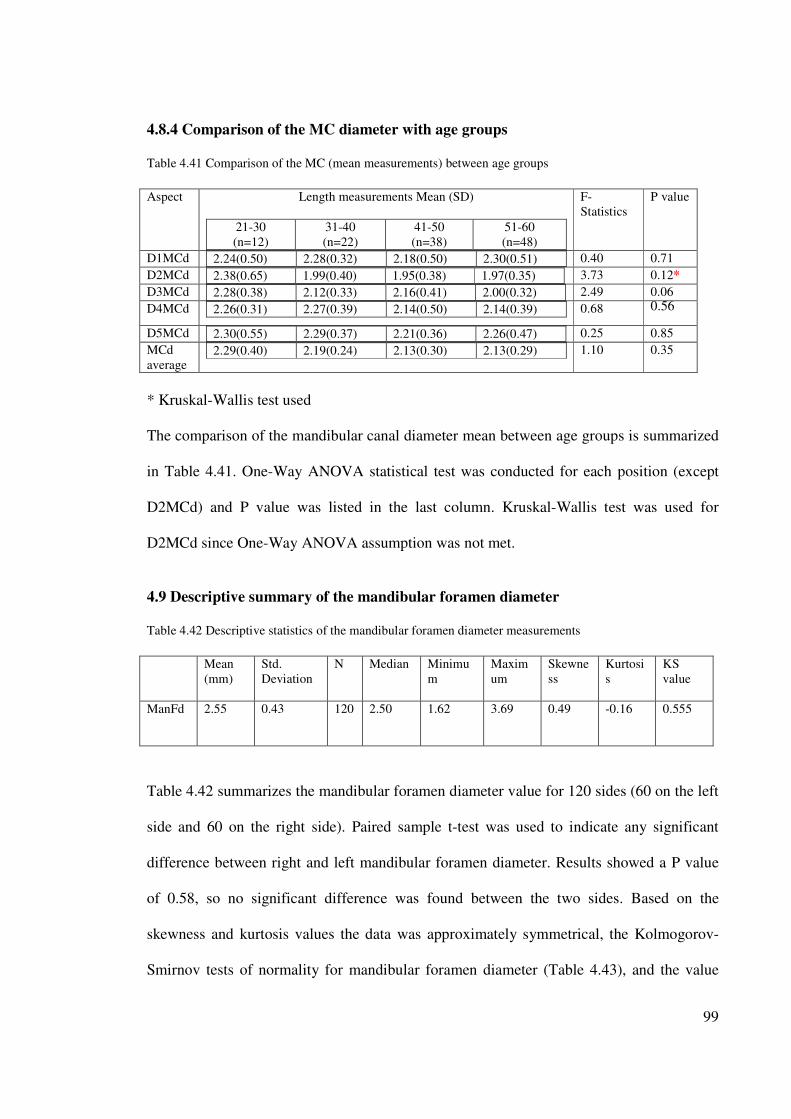
99
4.8.4 Comparison of the MC diameter with age groups
Table 4.41 Comparison of the MC (mean measurements) between age groups
Aspect Length measurements Mean (SD)
21-30
(n=12)
31-40
(n=22)
41-50
(n=38)
51-60
(n=48)
F-
Statistics
P value
D1MCd 2.24(0.50) 2.28(0.32) 2.18(0.50) 2.30(0.51)
0.40 0.71
D2MCd 2.38(0.65) 1.99(0.40) 1.95(0.38) 1.97(0.35)
3.73 0.12*
D3MCd 2.28(0.38) 2.12(0.33) 2.16(0.41) 2.00(0.32)
2.49 0.06
D4MCd 2.26(0.31) 2.27(0.39) 2.14(0.50) 2.14(0.39)
0.68 0.56
D5MCd 2.30(0.55) 2.29(0.37) 2.21(0.36) 2.26(0.47)
0.25 0.85
MCd
average 2.29(0.40) 2.19(0.24) 2.13(0.30) 2.13(0.29)
1.10 0.35
* Kruskal-Wallis test used
The comparison of the mandibular canal diameter mean between age groups is summarized
in Table 4.41. One-Way ANOVA statistical test was conducted for each position (except
D2MCd) and P value was listed in the last column. Kruskal-Wallis test was used for
D2MCd since One-Way ANOVA assumption was not met.
4.9 Descriptive summary of the mandibular foramen diameter
Table 4.42 Descriptive statistics of the mandibular foramen diameter measurements
Mean
(mm)
Std.
Deviation
N Median Minimu
m
Maxim
um
Skewne
ss
Kurtosi
s
KS
value
ManFd 2.55 0.43 120 2.50 1.62 3.69 0.49 -0.16 0.555
Table 4.42 summarizes the mandibular foramen diameter value for 120 sides (60 on the left
side and 60 on the right side). Paired sample t-test was used to indicate any significant
difference between right and left mandibular foramen diameter. Results showed a P value
of 0.58, so no significant difference was found between the two sides. Based on the
skewness and kurtosis values the data was approximately symmetrical, the Kolmogorov-
Smirnov tests of normality for mandibular foramen diameter (Table 4.43), and the value
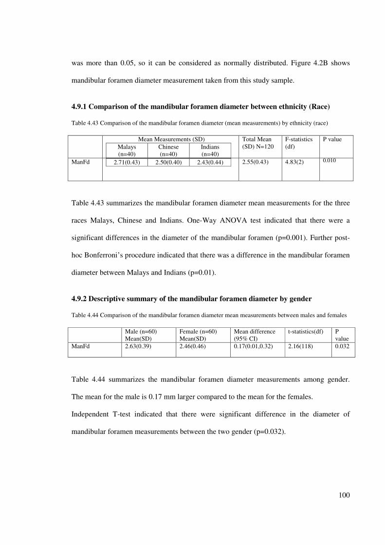
100
was more than 0.05, so it can be considered as normally distributed. Figure 4.2B shows
mandibular foramen diameter measurement taken from this study sample.
4.9.1 Comparison of the mandibular foramen diameter between ethnicity (Race)
Table 4.43 Comparison of the mandibular foramen diameter (mean measurements) by ethnicity (race)
Mean Measurements (SD)
Malays
(n=40)
Chinese
(n=40)
Indians
(n=40)
Total Mean
(SD) N=120
F-statistics
(df)
P value
ManFd 2.71(0.43) 2.50(0.40) 2.43(0.44)
2.55(0.43) 4.83(2) 0.010
Table 4.43 summarizes the mandibular foramen diameter mean measurements for the three
races Malays, Chinese and Indians. One-Way ANOVA test indicated that there were a
significant differences in the diameter of the mandibular foramen (p=0.001). Further post-
hoc Bonferroni’s procedure indicated that there was a difference in the mandibular foramen
diameter between Malays and Indians (p=0.01).
4.9.2 Descriptive summary of the mandibular foramen diameter by gender
Table 4.44 Comparison of the mandibular foramen diameter mean measurements between males and females
Male (n=60)
Mean(SD)
Female (n=60)
Mean(SD)
Mean difference
(95% CI)
t-statistics(df) P
value
ManFd 2.63(0.39) 2.46(0.46) 0.17(0.01,0.32) 2.16(118) 0.032
Table 4.44 summarizes the mandibular foramen diameter measurements among gender.
The mean for the male is 0.17 mm larger compared to the mean for the females.
Independent T-test indicated that there were significant difference in the diameter of
mandibular foramen measurements between the two gender (p=0.032).
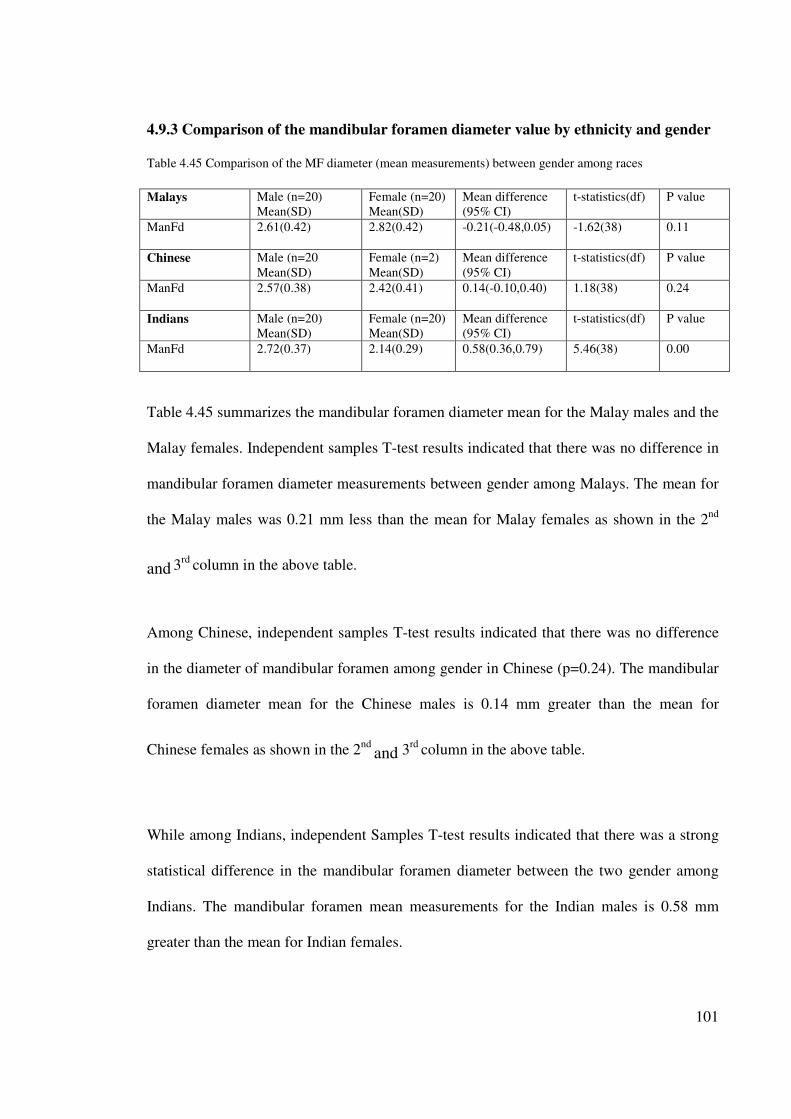
101
4.9.3 Comparison of the mandibular foramen diameter value by ethnicity and gender
Table 4.45 Comparison of the MF diameter (mean measurements) between gender among races
Malays Male (n=20)
Mean(SD)
Female (n=20)
Mean(SD)
Mean difference
(95% CI)
t-statistics(df) P value
ManFd 2.61(0.42) 2.82(0.42) -0.21(-0.48,0.05) -1.62(38) 0.11
Chinese Male (n=20
Mean(SD)
Female (n=2)
Mean(SD)
Mean difference
(95% CI)
t-statistics(df) P value
ManFd 2.57(0.38) 2.42(0.41) 0.14(-0.10,0.40) 1.18(38) 0.24
Indians Male (n=20)
Mean(SD)
Female (n=20)
Mean(SD)
Mean difference
(95% CI)
t-statistics(df) P value
ManFd 2.72(0.37) 2.14(0.29) 0.58(0.36,0.79) 5.46(38) 0.00
Table 4.45 summarizes the mandibular foramen diameter mean for the Malay males and the
Malay females. Independent samples T-test results indicated that there was no difference in
mandibular foramen diameter measurements between gender among Malays. The mean for
the Malay males was 0.21 mm less than the mean for Malay females as shown in the 2nd
and 3rd
column in the above table.
Among Chinese, independent samples T-test results indicated that there was no difference
in the diameter of mandibular foramen among gender in Chinese (p=0.24). The mandibular
foramen diameter mean for the Chinese males is 0.14 mm greater than the mean for
Chinese females as shown in the 2nd
and 3rd
column in the above table.
While among Indians, independent Samples T-test results indicated that there was a strong
statistical difference in the mandibular foramen diameter between the two gender among
Indians. The mandibular foramen mean measurements for the Indian males is 0.58 mm
greater than the mean for Indian females.
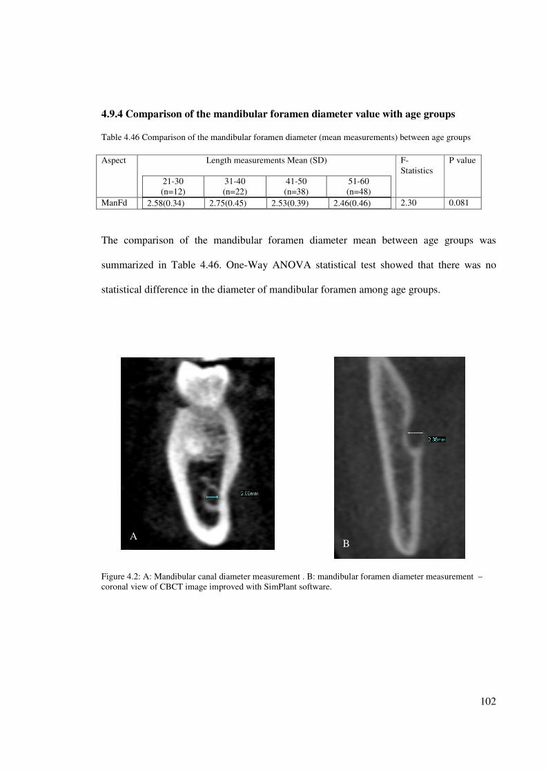
102
4.9.4 Comparison of the mandibular foramen diameter value with age groups
Table 4.46 Comparison of the mandibular foramen diameter (mean measurements) between age groups
Aspect Length measurements Mean (SD)
21-30
(n=12)
31-40
(n=22)
41-50
(n=38)
51-60
(n=48)
F-
Statistics
P value
ManFd 2.58(0.34) 2.75(0.45) 2.53(0.39) 2.46(0.46)
2.30 0.081
The comparison of the mandibular foramen diameter mean between age groups was
summarized in Table 4.46. One-Way ANOVA statistical test showed that there was no
statistical difference in the diameter of mandibular foramen among age groups.
Figure 4.2: A: Mandibular canal diameter measurement . B: mandibular foramen diameter measurement –
coronal view of CBCT image improved with SimPlant software.
A B
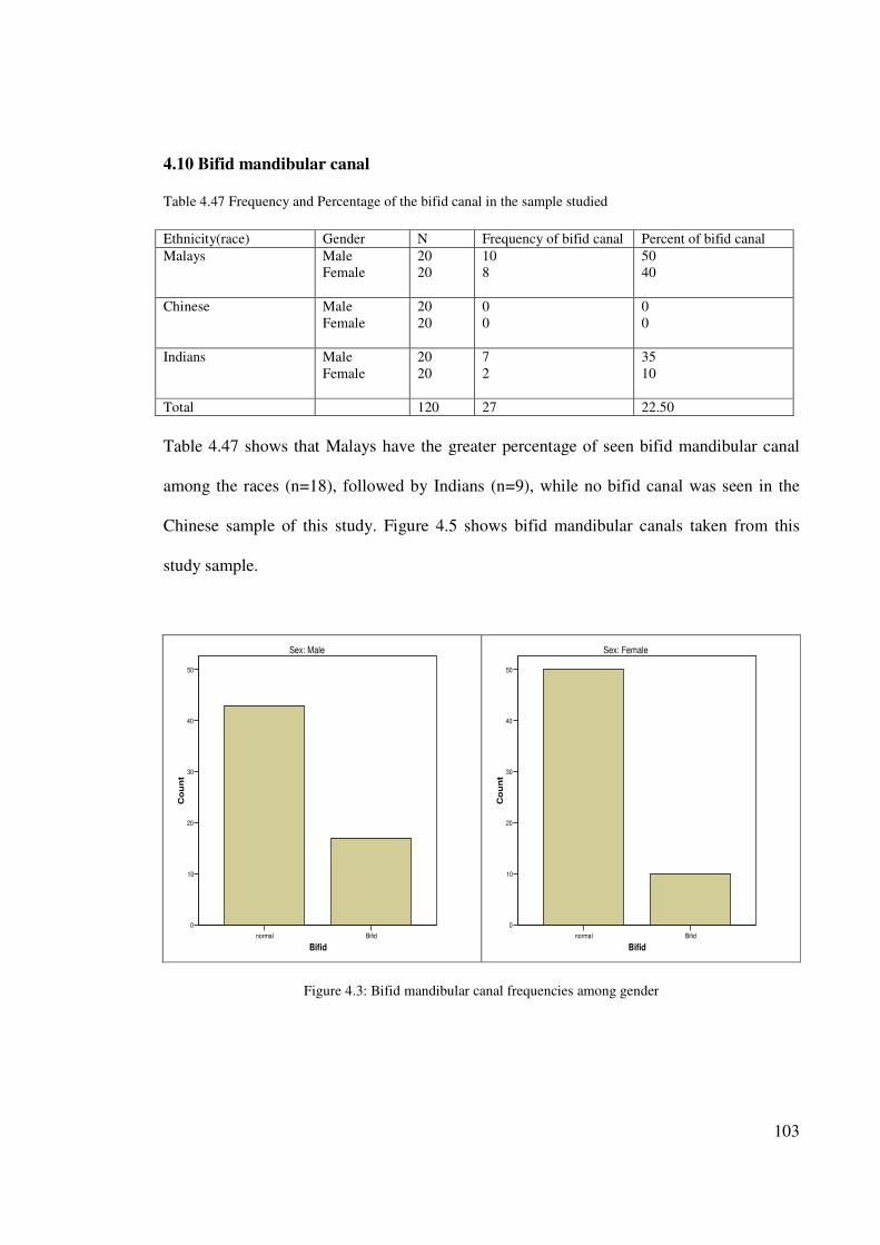
103
4.10 Bifid mandibular canal
Table 4.47 Frequency and Percentage of the bifid canal in the sample studied
Ethnicity(race) Gender N Frequency of bifid canal Percent of bifid canal
Malays Male
Female
20
20
10
8
50
40
Chinese Male
Female
20
20
0
0
0
0
Indians Male
Female
20
20
7
2
35
10
Total 120 27 22.50
Table 4.47 shows that Malays have the greater percentage of seen bifid mandibular canal
among the races (n=18), followed by Indians (n=9), while no bifid canal was seen in the
Chinese sample of this study. Figure 4.5 shows bifid mandibular canals taken from this
study sample.
normal Bifid
Bifid
0
10
20
30
40
50
Co
un
t
Sex: Male
normal Bifid
Bifid
0
10
20
30
40
50
Co
un
t
Sex: Female
Figure 4.3: Bifid mandibular canal frequencies among gender
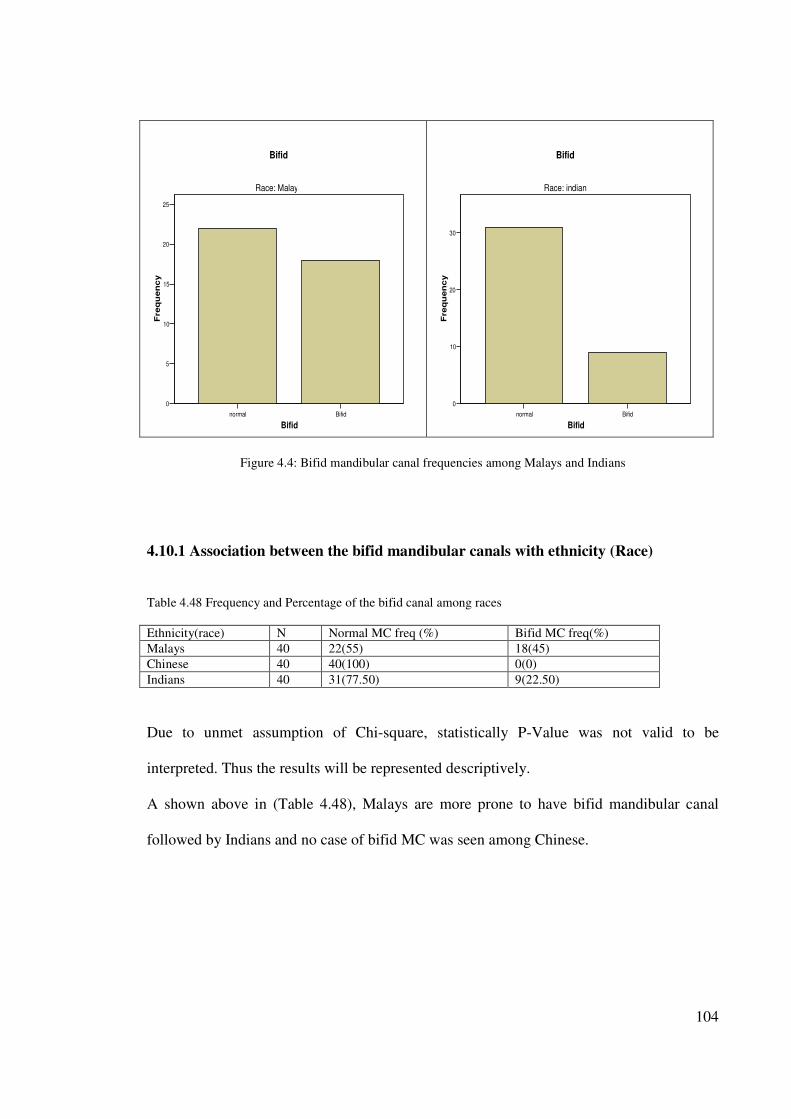
104
normal Bifid
Bifid
0
5
10
15
20
25
Fre
qu
en
cy
Race: Malaya
Bifid
normal Bifid
Bifid
0
10
20
30
Fre
qu
en
cy
Race: indian
Bifid
Figure 4.4: Bifid mandibular canal frequencies among Malays and Indians
4.10.1 Association between the bifid mandibular canals with ethnicity (Race)
Table 4.48 Frequency and Percentage of the bifid canal among races
Ethnicity(race) N Normal MC freq (%) Bifid MC freq(%)
Malays 40 22(55) 18(45)
Chinese 40 40(100) 0(0)
Indians 40 31(77.50) 9(22.50)
Due to unmet assumption of Chi-square, statistically P-Value was not valid to be
interpreted. Thus the results will be represented descriptively.
A shown above in (Table 4.48), Malays are more prone to have bifid mandibular canal
followed by Indians and no case of bifid MC was seen among Chinese.
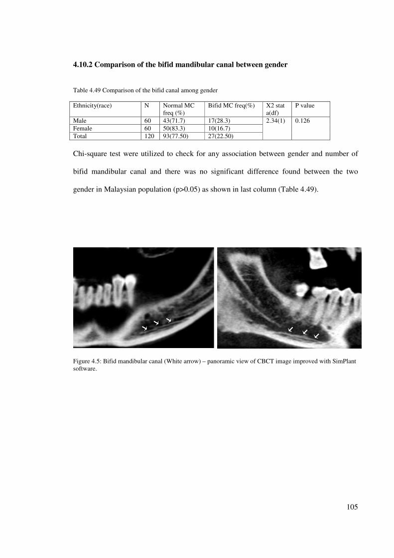
105
4.10.2 Comparison of the bifid mandibular canal between gender
Table 4.49 Comparison of the bifid canal among gender
Ethnicity(race) N Normal MC
freq (%)
Bifid MC freq(%) X2 stat
a(df)
P value
Male 60 43(71.7) 17(28.3) 2.34(1) 0.126
Female 60 50(83.3) 10(16.7)
Total 120 93(77.50) 27(22.50)
Chi-square test were utilized to check for any association between gender and number of
bifid mandibular canal and there was no significant difference found between the two
gender in Malaysian population (p>0.05) as shown in last column (Table 4.49).
Figure 4.5: Bifid mandibular canal (White arrow) – panoramic view of CBCT image improved with SimPlant
software.
106
CHAPTER 5
DISCUSSION
5.1 Rational for choice of the study topic
The current study was designed to clearly determine the path of the mandibular canal, the
mandibular canal diameter, the mandibular foramen diameter and the frequency of bifid
mandibular canal in Malaysian population using appropriate application of CBCT and
SimPlant software.
The presence and contents of the neurovascular bundles were clearly identified in studies
done by Deng et al.(2008), using High-Resolution Magnetic Resonance Imaging (HR-
MRI). As such the function and importance of those structures became evident and their
correlation to the majority of the pre-surgical and post-surgical complications that occurred
in the mandibular region was better understood.
The choice of this topic was based on four reasons. Firstly, a perusal of data and records
revealed that no such studies had previously been done in a Malaysian population and
therefore the present study would act as a pilot to lay down primary data on the mandibular
canal pathway among Malay, Chinese and Indians. Dentists worldwide who are treating
people of Malaysian origin can then use this data.
107
Secondly, the number of practitioners performing implant surgery has increased
dramatically over the last fifteen years. As confidence is gained they tend to accept
increasingly challenging cases and it is to be expected that the incidence of problems and
complications will increase (Worthington, 1995).
Thirdly, studies showed that IAN is the most commonly injured nerve in the mandible
(64.4%), followed by the lingual nerve (28.8%) (Tay and Zuniga, 2007).
Lastly, the use of CBCT as the imaging technique was chosen as it is non-invasive, emits
low radiation and has been successfully applied in several areas of dentistry such as oral
surgery, endodontics, oral medicine, periodontology, restorative dentistry and orthodontics
(Rigolone et al., 2003, Nakagawa et al., 2002, Hamada et al., 2005, Ogawa et al., 2005,
Maki et al., 2003, Hatcher et al., 2003, Sato et al., 2004, Tsiklakis et al., 2004).
Though intra-oral radiographs have remained the most popular in dental clinics for a long
time and have been used in some studies (Denio et al., 1992), the technique is limited by
the fact that images are produced only in 2D. Furthermore, such images if taken on patients
could be elongated or shortened thus compounding the actual size of the specimen under
study. In addition, superimposition of structures could occur. On the other hand, CBCT
produced 3D images with no geometrical distortion since the image is at a ratio of l:1,
implying that the image produced is the same size as the object. Furthermore, there is good
resolution and problems of superimposition can be eliminated.
108
CT has also been used to improve depiction of the mandibular canal (Naitoh et al., 2008,
Yang et al., 1999) .However, compared to CBCT, CT equipment has been found to be very
bulky, emitted high radiation and scatter, and are quite expensive. The use of CBCT in oral
and maxillofacial surgery has been well documented as stated earlier. However, a paucity
of data exists on its use to determine the mandibular canal metrical path analyses hence it’s
the choice for the present study.
5.2 Limitations of the study
As many number of measurements were required, the sample size of the CBCT records
were limited to sixty patients (bilateral measurements – 120). Even though the results of
this study were statistically relevant some may consider the sample size used was not
sufficiently large. This study also deals mainly with CBCT record transfer and the
application of the SimPlant software programs to produce accurate jaw simulation of
relevant structures.
It was therefore necessary to have vast knowledge and expertise in the anatomy of the jaw
as well as be competent in images interpretation in order to accurately identify the required
structures during 3D simulation.
5.3 Specimen selection
A total of sixty (60) suitable patients records were selected based on gender, ethnicity and
age groups. Males or females from racial groups, Malays, Chinese and Indians aged
between twenty (20) and sixty (60) with permanent dentition were included since most
patient seeking implant treatment in this age period. Also patients with systemic health
109
problems or are medically compromised and not having undergone any radiotherapy were
also included.
While samples with mixed racial origin, with history of severe trauma or fracture of the
mandible, existing pathological disorder at mandible, with genetic disorder or congenital
abnormalities, samples with post surgical cases such as orthognathic surgery, or samples
with severely atrophied mandible were excluded from the sample collection. The exclusion
criteria in this study were very strict to get an ideal sample size that provides excellent
results and that is why it took long period for proper sample selection.
5.4 Technique
5.4.1 The imaging system
CBCT was chosen as the imaging technique of choice since it has been documented to
provide excellent 3-dimensional images at reduced radiation scan time and cost in clinical
studies (Yajima et al., 2006, Ziegler et al., 2002, Schramm et al., 2005, Scarfe et al., 2006).
In addition CBCT was shown in some clinical studies to be more accurate and provided
higher resolution compared to CT (Cotton et al., 2007). It is comparable to direct digital
caliper measurements of various distances surrounding the mandibular canal (Kamburoglu
et al., 2009) and was found to be reliable for linear evaluation measurements of structures
closely associated with dental and maxillofacial imaging (Lascala et al., 2004).
SimPlant software tools allow the marking to be done in any of the axial, cross sectional,
panoramic and 3D view. It also permitted scrolling through the entire volume with
simultaneous viewing of axial, coronal and sagital sections.
110
5.4.2 Landmarks, Base line and Measurements
The mandibular canal was used as landmark for measurements in most of the cadaveric and
radiographic studies. However, cadavers are processed specimen and fixed in formalin and
because of this the nerve (being soft tissues) is prone to deformation and therefore becomes
an inexact landmark. In contrast radiographic studies, the presence of cortical lining
forming the wall of the mandibular canal act as a factor for their visualization (Rothman et
al., 1988). Cone-Beam computed tomography allows a precise demonstration of the
mandibular canal in relation to the alveolar crest, inferior border and bucco-lingual
directions of the mandible.
We adapted the diameter of the canal to be 2.50 mm in our metrical studies of the position
of the canal and this was set as default in the SimPlant software program. This was done as
this was the diameter reported by Rajchel et al. in a study in 1986.
5.4.3 Reliable landmarks for mandibular canal position
The CBCT images selected in this study were all taken with Frankfort plane parallel to the
floor. The interactive SimPlant software was used to produce dynamic high resolution
cross-sectional and 3-D images, which allowed the visualization of the mandibular canal
from any viewpoint on the computer screen.
The SimPlant software allows access to a measurement tools for linear measurements of the
mandibular canal. The main concern in this study was selecting appropriate landmarks and
base lines to allow optimum standardization and reproducibility.
111
The buccal line, lingual line, inferior line and superior line were introduced and selected as
base lines in the present study. The preliminary studies showed good standardization and
reproducibility of the base lines and measurements. The data analyzed for reliability of the
measurements showed Cronbach alpha coefficient as r=0.91, and the value of measurement
errors, s(i) were 0.05 mm or less for all compared data, which strongly suggested the
present method of obtaining data is considered as reliable and accurate.
The superior aspect for D5 was excluded from this study because there was no superior
alveolar crest (only ramus) and there was no way of determining the superior margin as
done in other locations.
5.5 Comparison of data between right and left jaw
One of the objectives of this research is to study the significance of data collected from
right and left side of the mandible and to determine whether it is suitable to use data from
both side of the jaw in conducting clinical researches. The mean values obtained for right
and left sides of all D’s (D1-D5) were identical and the P-values of the pair-samples T-test
showed a value of more than 0.05 (Table 4.1).
This result strongly concludes that the measures on the right are similar to the measures on
the left side of the jaw as also stated by Levine et al. (2007), Narayana and Vasudha (2004)
and Kieser et al. (2005). Recording the measurement on both sides of the jaw in clinical
studies may then produce cluster sampling as well as duplication of the data, which then
becomes unnecessary in metrical analyses. One side is therefore sufficient in future studies.
112
5.6 Position of the mandibular canal
In this study the position of the mandibular canal at all D’s (D1-D5) location were
measured at four aspects which are the buccal, lingual, inferior and superior measurements
respectively (except D5S), and statistical comparison were done based on race, gender, race
versus gender and age groups.
5.6.1 Apicocoronal position of the mandibular canal
Many studies were done to measure and locate mandibular canal position using different
imaging techniques ranging from periapical radiography to CBCT technique (Table 5.1).
One of the interesting clinical and radiographic study among US population was done by
Levine et al. (2007) using the CT imaging technique. They reported that the mandibular
canal was 17.4 ± 3.00 mm from the superior cortical surfaces of the mandible at the
mandibular first molar.
In this study the superior measurement of the position of the mandibular canal was 14.85 ±
3.64 mm at D1, 13.94 ± 3.85 mm at D2, 12.99 ± 4.08 mm at D3 and 14.22 ± 1.52 mm at
D4, while the inferior measurement of the canal was 9.37 ± 1.69 mm at D1, 8.24 ± 1.69
mm at D2, 7.96 ± 1.93 mm at D3, 9.65 ± 2.54 at D4 and 15.21 ± 4.18 mm at D5.
Ensuing a study on the vertical position of the mandibular canal, statistical comparisons
were done based on race and gender. According to race comparison, it was found that there
was no significant difference in the location of the canal at D1 position superiorly.
However, when we advance posteriorly in the mandible there was an obvious variation of
the position of the canal amongst the races especially from the inferior border of the
mandibular canal to the mandibular base until D5I where subsequently no significant
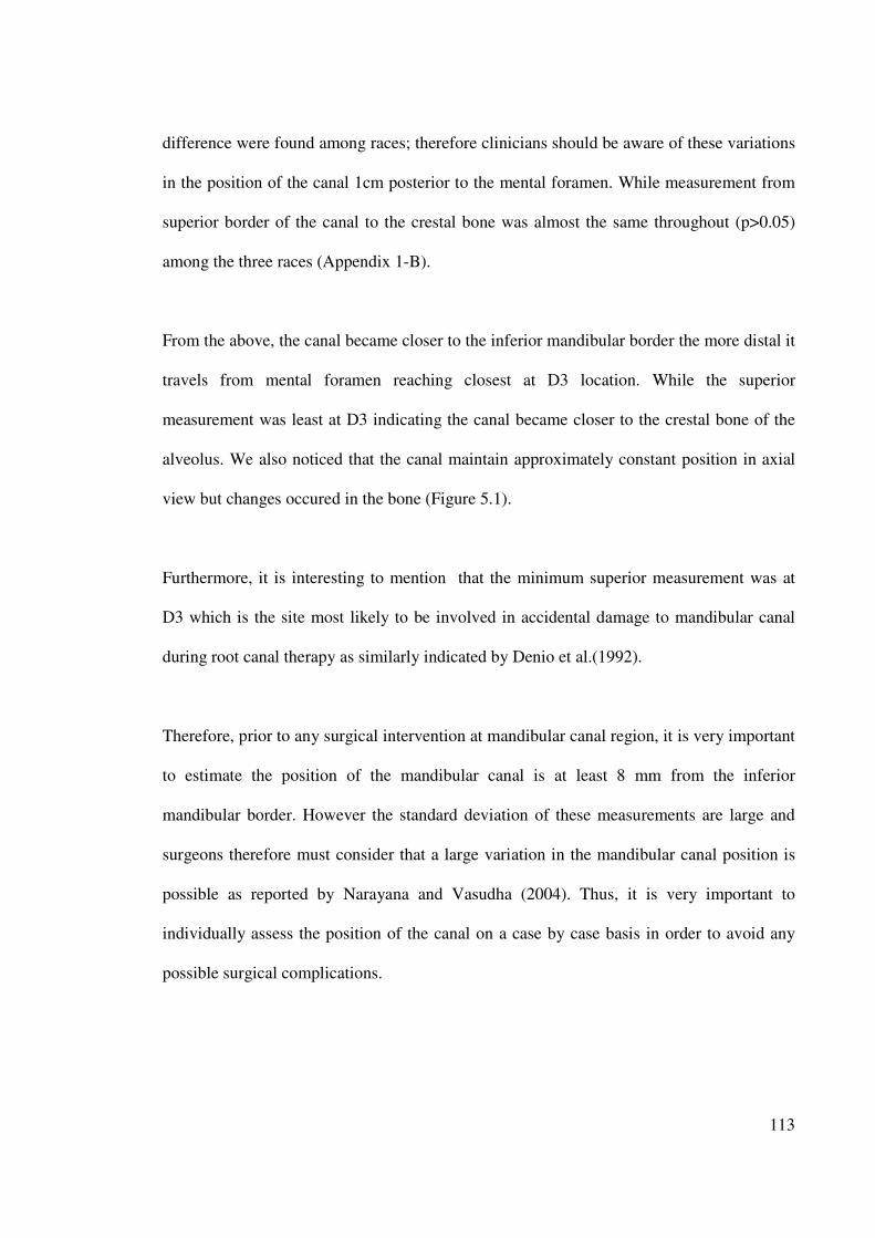
113
difference were found among races; therefore clinicians should be aware of these variations
in the position of the canal 1cm posterior to the mental foramen. While measurement from
superior border of the canal to the crestal bone was almost the same throughout (p>0.05)
among the three races (Appendix 1-B).
From the above, the canal became closer to the inferior mandibular border the more distal it
travels from mental foramen reaching closest at D3 location. While the superior
measurement was least at D3 indicating the canal became closer to the crestal bone of the
alveolus. We also noticed that the canal maintain approximately constant position in axial
view but changes occured in the bone (Figure 5.1).
Furthermore, it is interesting to mention that the minimum superior measurement was at
D3 which is the site most likely to be involved in accidental damage to mandibular canal
during root canal therapy as similarly indicated by Denio et al.(1992).
Therefore, prior to any surgical intervention at mandibular canal region, it is very important
to estimate the position of the mandibular canal is at least 8 mm from the inferior
mandibular border. However the standard deviation of these measurements are large and
surgeons therefore must consider that a large variation in the mandibular canal position is
possible as reported by Narayana and Vasudha (2004). Thus, it is very important to
individually assess the position of the canal on a case by case basis in order to avoid any
possible surgical complications.
114
Table 5.1 Comparison of studies locating the mandibular canal vertically
Authors N Materials &
Methods
Location of MC
(Heasman, 1988) 96 -Plain films
-Dried mandibles
68% MC passed along an intermediate course
between the mandibular root apices and the
IBM.
(Rajchel et al., 1986) 45 -Cadavers
-Cross-sectional
Mean distance of 10 mm between the MC and
the IMB, proximally to the third molar region.
(Littner et al., 1986) 46 -paralleling technique
radiography
Upper border of the MC to root apices of 6:
3.5mm
Upper border of the MC to root apices of 7:
5.4mm
(Denio et al., 1992) 22 -Cadavers
-Sectioning
MC to the apices of 7 : 3.7 mm
MC to the first molar : 6.90 mm
MC to premolars : 4.7 mm
(Sato et al., 2005) 39 - Macroscopic
cadaveric dissection
- CT or panoramic
X-ray observation
vertical position of MC was closer to the apices
of the first and the second molars than that to the
distance of the IBM
(Carter and Keen, 1971) 8
80
- Dissection
- Unilateral
radiographs
Classified the three vertical positions of the
course of the IAN. According to Type l, the
nerve has a course near the apices of the teeth,
where in Type ll, the main trunk is low down in
the body, finally type III, the main trunk is low
down in the body of the mandible with several
smaller branches to the molar teeth.
(Nortjĕ et al., 1977b) 3612 - Panoramic
radiograph
Categorized finding into: 1) 47% of cases high
MC (within 2mm of the apices of the 6 & 7), 2)
3% intermediate MC, 3) 49% of cases low MC,
and 4) other variations.
(Kieser et al., 2004) 39 micro-dissections In 30.7% of the cases, the IAN was located in
the superior part of the body of the mandible,
and in 69.3% of the cases the IAN was half-way
or closer to the inferior border of the mandible.
(Levine et al., 2007) 50 - Axial computed
tomography
- SimPlant software
superior aspect of the MC was 17.4 mm inferior
from the alveolar crest
(Watanabe et al., 2009) 79 cross-sectional CT
images
Distance from alveolar crest to the MC ranged
from 15.3 to 17.4 mm
Present study (2011) 120 - CBCT
- SimPlant software
D1/S : 14.85± 3.64 mm D1I : 9.37± 1.69mm
D2/S : 13.94± 3.85 mm D2I : 8.24± 1.69mm
D3/S : 12.99± 3.08 mm D3I : 7.96± 1.93mm
D4/S : 14.22± 4.02 mm D4I : 9.65± 2.54mm
D5/S: - D5I : 15.21± 4.18mm
115
Another interesting finding of this study when comparing mandibular canal position among
gender was that male mandibular canal was more coronal than females and in general
females had lesser measurements than males at D1, D2 and D3, while no significant
difference were found for the other positions among gender.
5.6.2 Buccolingual position of mandibular canal
This study is considered to be a benchmark study in the buccolingual location of the
mandibular canal. The data obtained from this study measures the thickness of the bone
buccal and lingual to the mandibular canal in 5 different locations along the course of the
canal.
According to Levine et al. (2007) mentioned earlier, the mandibular canal was 4.90 ± 1.3
mm from the buccal cortical surfaces of the mandible at the mandibular first molar (Table
5.2).
In this study statistical comparison for buccolingual position of the mandibular canal were
conducted based on race, gender, race versus gender and age group. A variety of significant
differences were observed among the three races and the two gender according to their
measurements (Appendix 1-C). The obtained mean for the position of mandibular canal
were 3.89 ± 1.00 mm (buccal) and 4.33 ± 1.25 mm (lingual), 5.59 ± 1.20 mm (buccal) and
3.35 ± 1.20 mm (lingual), 6.71 ± 1.34 mm (buccal) and 3.25 ± 1.32 mm (lingual), 5.68 ±
1.63 mm (buccal) and 3.08 ± 1.46 mm (lingual), 4.24 ± 1.59 mm (buccal) and 2.12 ± 1.40
mm (lingual) at D1,D2,D3,D4 and D5 respectively.
116
From the above findings, it was noted that the buccal distance increased until D3 after
which it is reduced while lingual distance reduced all the way from D1 to D5. As such the
mandibular canal deviates more lingually the more distal the canal travels, with its lowest
reading lingually at D4 (30 mm from the mental foramen) (2.12 ± 1.4 mm) (Figures 5.1 and
5.2). Thus, prior to any surgical intervention at this area, this research demonstrated that the
buccal aspect of the mandibular canal has more bone material than on the lingual aspect. As
mentioned earlier because the standard deviation of the measurement in this study is large
so surgeons must consider that the variation in the mandibular canal position to be quite
evident and it is crucial to individually assess the position of the mandibular canal bucco-
lingually on a case-by-case basis.
It is interesting to mention that Chinese (7.07 ± 1.38 mm) had the largest buccal bone mean
measurement among the three races, followed by Malays (6.84 ± 1.22 mm), and the lowest
value was obtained from Indians (3.43 ± 0.88 mm). Again Chinese too had the largest
lingual bone measurement among the three races (4.39 ± 1.10 mm), followed by Malays
(4.38 ± 1.29 mm), and the lowest value was noticed among the Indians samples (2.10 ±
1.49 mm).
Another interesting finding from this study on the measurement among the races was that
the buccal measurement was statistically different (p<0.05) while lingual measurement
were almost the same with no much statistical difference except at D3L location (p=0.02).
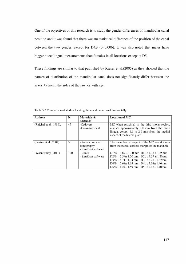
117
One of the objectives of this research is to study the gender differences of mandibular canal
position and it was found that there was no statistical difference of the position of the canal
between the two gender, except for D4B (p=0.006). It was also noted that males have
bigger buccolingual measurements than females in all locations except at D5.
These findings are similar to that published by Kieser et al.(2005) as they showed that the
pattern of distribution of the mandibular canal does not significantly differ between the
sexes, between the sides of the jaw, or with age.
Table 5.2 Comparison of studies locating the mandibular canal horizontally
Authors N Materials &
Methods
Location of MC
(Rajchel et al., 1986), 45 -Cadavers
-Cross-sectional
MC when proximal to the third molar region,
courses approximately 2.0 mm from the inner
lingual cortex, 1.6 to 2.0 mm from the medial
aspect of the buccal plate.
(Levine et al., 2007) 50 - Axial computed
tomography
- SimPlant software
The mean buccal aspect of the MC was 4.9 mm
from the buccal cortical margin of the mandible
Present study (2011) 120 - CBCT
- SimPlant software
D1/B : 3.89 ± 1.00 mm D1L : 4.33 ± 1.25mm
D2/B : 5.59± 1.20 mm D2L : 3.35 ± 1.20mm
D3/B : 6.71± 1.34 mm D3L : 3.25± 1.32mm
D4/B : 5.68± 1.63 mm D4L : 3.08± 1.46mm
D5/B : 4.24± 1.59 mm D5L : 2.12± 1.40mm
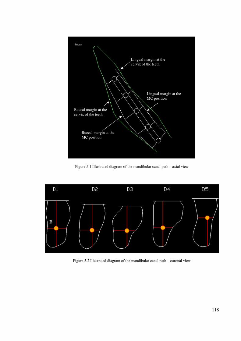
118
Figure 5.1 Illustrated diagram of the mandibular canal path – axial view
Figure 5.2 Illustrated diagram of the mandibular canal path – coronal view
Buccal margin at the
cervix of the teeth
Buccal margin at the
MC position
Buccal
Lingual margin at the
cervix of the teeth
Lingual margin at the
MC position
B
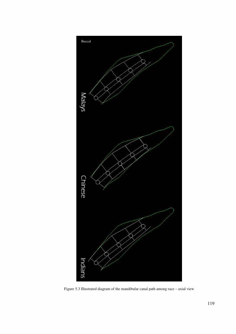
119
Figure 5.3 Illustrated diagram of the mandibular canal path among race – axial view
Buccal
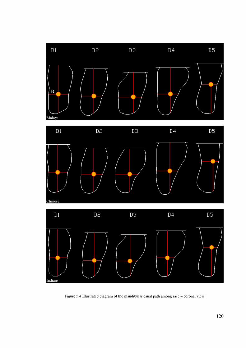
120
Figure 5.4 Illustrated diagram of the mandibular canal path among race – coronal view
Malays
Chinese
Indians
B
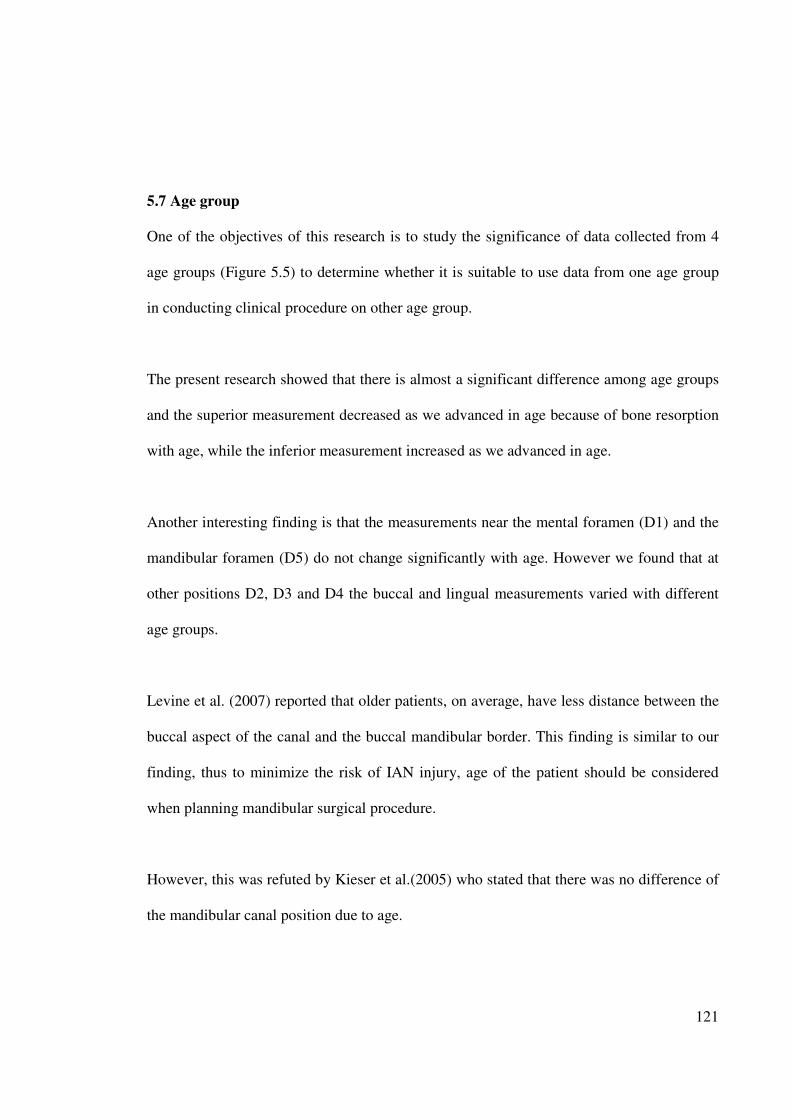
121
5.7 Age group
One of the objectives of this research is to study the significance of data collected from 4
age groups (Figure 5.5) to determine whether it is suitable to use data from one age group
in conducting clinical procedure on other age group.
The present research showed that there is almost a significant difference among age groups
and the superior measurement decreased as we advanced in age because of bone resorption
with age, while the inferior measurement increased as we advanced in age.
Another interesting finding is that the measurements near the mental foramen (D1) and the
mandibular foramen (D5) do not change significantly with age. However we found that at
other positions D2, D3 and D4 the buccal and lingual measurements varied with different
age groups.
Levine et al. (2007) reported that older patients, on average, have less distance between the
buccal aspect of the canal and the buccal mandibular border. This finding is similar to our
finding, thus to minimize the risk of IAN injury, age of the patient should be considered
when planning mandibular surgical procedure.
However, this was refuted by Kieser et al.(2005) who stated that there was no difference of
the mandibular canal position due to age.
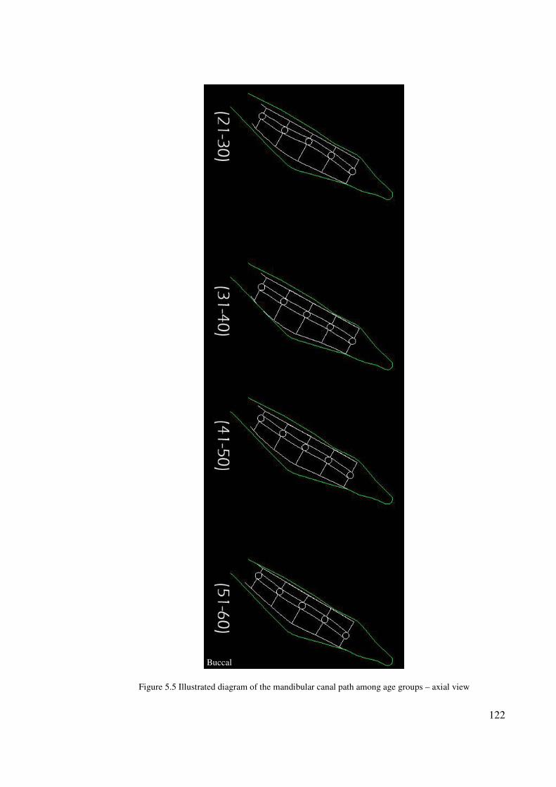
122
Figure 5.5 Illustrated diagram of the mandibular canal path among age groups – axial view
Buccal
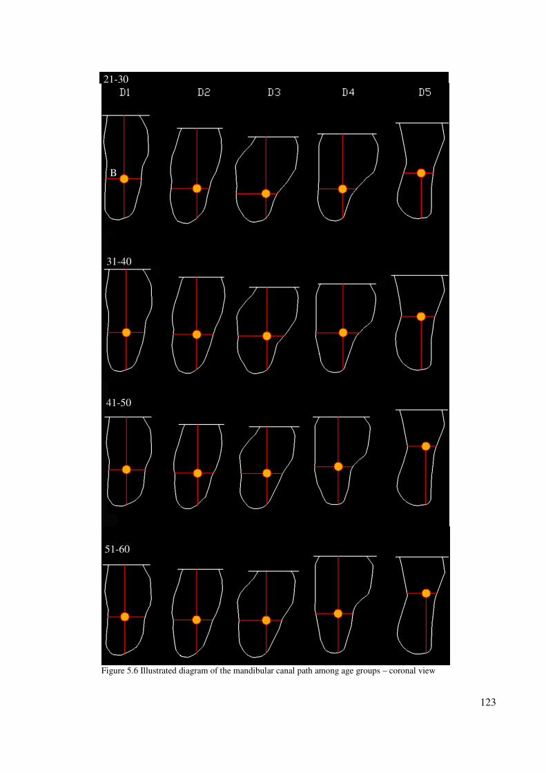
123
Figure 5.6 Illustrated diagram of the mandibular canal path among age groups – coronal view
41-50
31-40
51-60
21-30
B
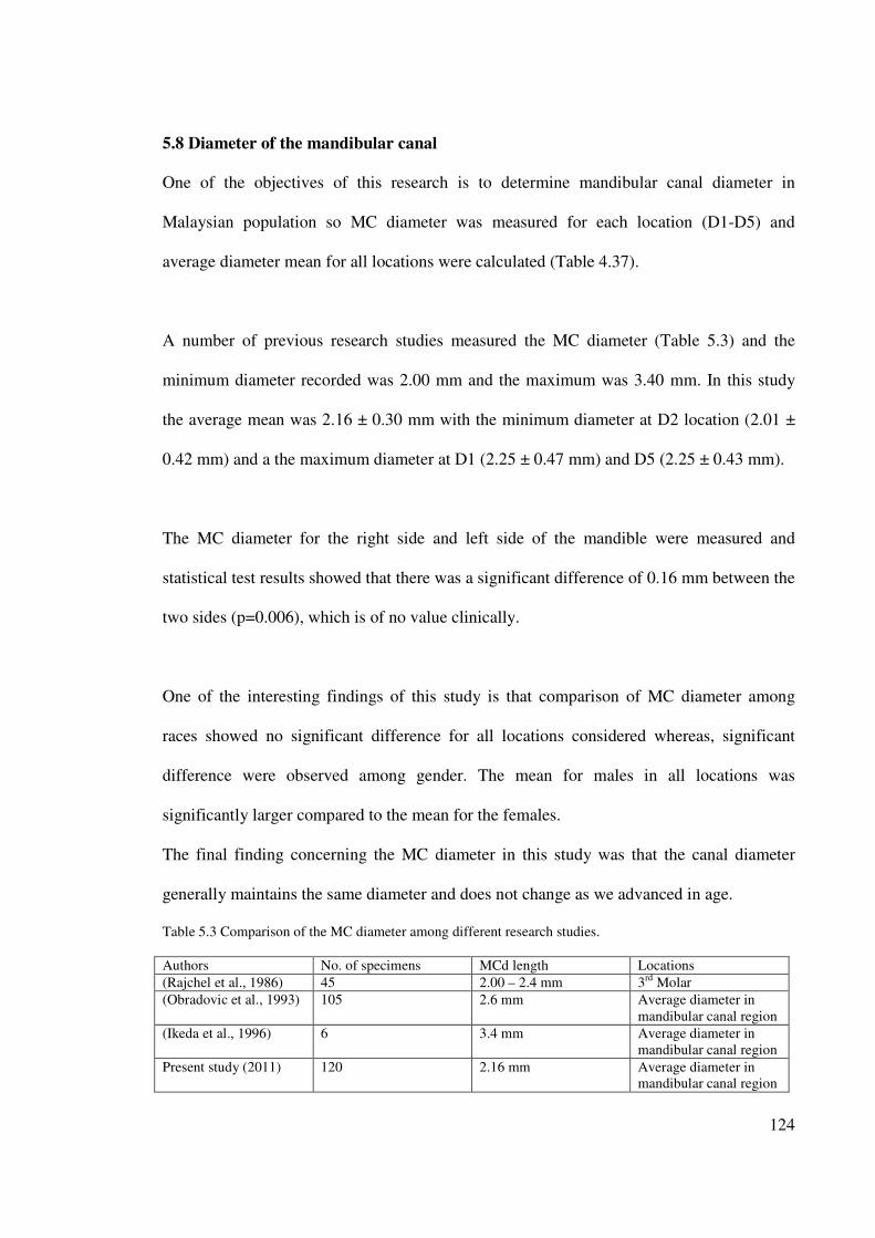
124
5.8 Diameter of the mandibular canal
One of the objectives of this research is to determine mandibular canal diameter in
Malaysian population so MC diameter was measured for each location (D1-D5) and
average diameter mean for all locations were calculated (Table 4.37).
A number of previous research studies measured the MC diameter (Table 5.3) and the
minimum diameter recorded was 2.00 mm and the maximum was 3.40 mm. In this study
the average mean was 2.16 ± 0.30 mm with the minimum diameter at D2 location (2.01 ±
0.42 mm) and a the maximum diameter at D1 (2.25 ± 0.47 mm) and D5 (2.25 ± 0.43 mm).
The MC diameter for the right side and left side of the mandible were measured and
statistical test results showed that there was a significant difference of 0.16 mm between the
two sides (p=0.006), which is of no value clinically.
One of the interesting findings of this study is that comparison of MC diameter among
races showed no significant difference for all locations considered whereas, significant
difference were observed among gender. The mean for males in all locations was
significantly larger compared to the mean for the females.
The final finding concerning the MC diameter in this study was that the canal diameter
generally maintains the same diameter and does not change as we advanced in age.
Table 5.3 Comparison of the MC diameter among different research studies.
Authors No. of specimens MCd length Locations
(Rajchel et al., 1986) 45 2.00 – 2.4 mm 3rd
Molar
(Obradovic et al., 1993) 105 2.6 mm Average diameter in
mandibular canal region
(Ikeda et al., 1996) 6 3.4 mm Average diameter in
mandibular canal region
Present study (2011) 120 2.16 mm Average diameter in
mandibular canal region
125
5.9 Diameter of the mandibular foramen
One of the objectives of this research was to determine the mandibular foramen diameter in
Malaysian population and this was measured to be having a diameter of 2.55 ± 0.43 mm.
The MF diameter for the right side and left side of the mandible were measured and
statistical test results showed that no significant difference was found between the two sides
(p=0.241).
Comparison of the MF diameter among races indicated that there was a difference in the
mandibular foramen diameter between Malay and Indian races (p=0.01). Furthermore
comparison of the MF diameter among gender indicated that there were significant
difference in the diameter of the mandibular foramen measurement (p=0.032) with males
showing larger values.
One of the interesting findings of this study is that the MF diameter generally maintains the
same diameter and does not change as Malaysians advanced in age. This finding is similar
to MC diameter with age group mentioned earlier.
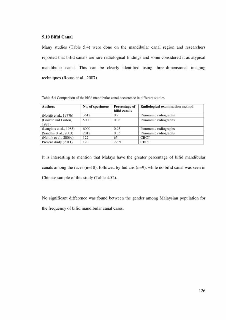
126
5.10 Bifid Canal
Many studies (Table 5.4) were done on the mandibular canal region and researchers
reported that bifid canals are rare radiological findings and some considered it as atypical
mandibular canal. This can be clearly identified using three-dimensional imaging
techniques (Rouas et al., 2007).
Table 5.4 Comparison of the bifid mandibular canal occurrence in different studies
Authors No. of specimens Percentage of
bifid canals
Radiological examination method
(Nortjĕ et al., 1977b) 3612 0.9 Panoramic radiographs
(Grover and Lorton,
1983)
5000 0.08 Panoramic radiographs
(Langlais et al., 1985) 6000 0.95 Panoramic radiographs
(Sanchis et al., 2003) 2012 0.35 Panoramic radiographs
(Naitoh et al., 2009a) 122 65 CBCT
Present study (2011) 120 22.50 CBCT
It is interesting to mention that Malays have the greater percentage of bifid mandibular
canals among the races (n=18), followed by Indians (n=9), while no bifid canal was seen in
Chinese sample of this study (Table 4.52).
No significant difference was found between the gender among Malaysian population for
the frequency of bifid mandibular canal cases.
127
CHAPTER 6
CONCLUSION, IMPLICATIONS AND SUGGESTIONS
6.1 Introduction
This study investigated the metrical path way of the mandibular canal among Malaysian
population at every 10 mm starting from the mental foramen backward. There was also an
attempt to determine the MC diameter at each location, MF diameter and frequency of bifid
canal. The following are the summary of findings, implications of the study as well as
recommendations for further studies.
6.2 Summary of the findings
The research was specifically focused to study six objectives and the results obtained were
as follows:
(i) The mandibular canal was identified as a major big canal in all the samples with
100% superb visibility.
(ii) The inferior border of the mandible showed high reliability as a landmark for
mandibular incisive canal position.
(iii) The mean apicocoronal position of the mandibular canal was 10.08 mm from
the inferior border of the mandible and 14.00 mm from the alveolar crestal bone.
128
Mandibular canal curving downward towards the inferior mandibular border
untill D3 and then it curves upwards.
(iv) The mean buccolingual position of the mandibular canal was 5.22 mm away
from the buccal cortical plate and 3.65 mm away from the lingual cortical plate.
The mandibular canal curves toward the lingual side the more distally we
measure the MC away from mental foramen.
(v) The mean mandibular canal diameter was 2.16 ± 0.30 mm in the Malaysian
population.
(vi) The mean mandibular foramen diameter was 2.55 ± 0.43 mm in the Malaysian
population.
(vii) Bifid mandibular canal was identified using CBCT technology with prevalence
of 22.50% in the Malaysian population.
(viii) The data from the right side of the jaw were approximately similar to the data
from the left side of the jaw for all measured structures in this study.
(ix) CBCT proved a reliable means of analyzing mandibular canal position,
determining MC and MF diameter and distinguishing the bifid canal.
129
6.3 Implications of the study
The research clearly showed variations in the position of the mandibular canal and it
should not be assumed that there is a fixed position at which it is safe for surgical
intervention. Thus, it is highly recommended that the surgeons familiarize themselves
with the anatomic variation at the mandibular canal region prior to any surgical
intervention in order to avoid hemorrhage or neurosensory disturbances, as well as to
safeguard themselves from unexpected medicolegal complications. Computed
Tomography or cone beam computed tomography (CBCT) is recommended for
preoperative planning to overcome the shortfalls observed in other radiography.
6.4 Recommendations for further research
Many studies have attempted to measure or estimate the amount of radiation doses
delivered to radiosensitive organs in the maxillofacial area, such as salivary gland thus,
the risk of the ionizing radiation involved with radiographic techniques has been widely
investigated. The CBCT has a very short exposure time (10-70) seconds and radiation
dosage is 15 times less than the conventional CT scan.
Deng et al. (2008) have recommended the use of High Resolution Magnetic Resonance
Imaging (HR-MRI) to investigate the neurovascularization of the anterior jaw bone and
surrounding soft tissue. It is similarly recommended using HR-MRI or ultrasound to
visualize the canal in the Malaysian population. These imaging modalities do not use
ionizing radiation and are considered non-invasive.

130
6.5 Closure
As a healthcare provider, it is our ethical duty to provide a harmless treatment to our
patients. We have to anticipate and recognize the neurovascularization of the mandible to
avoid or minimize any complications. Great care must be considered as these vasculatures
are more complex and more variable than previously thought. Constant development of
modern imaging modalities has improved tremendously our diagnostic capabilities.
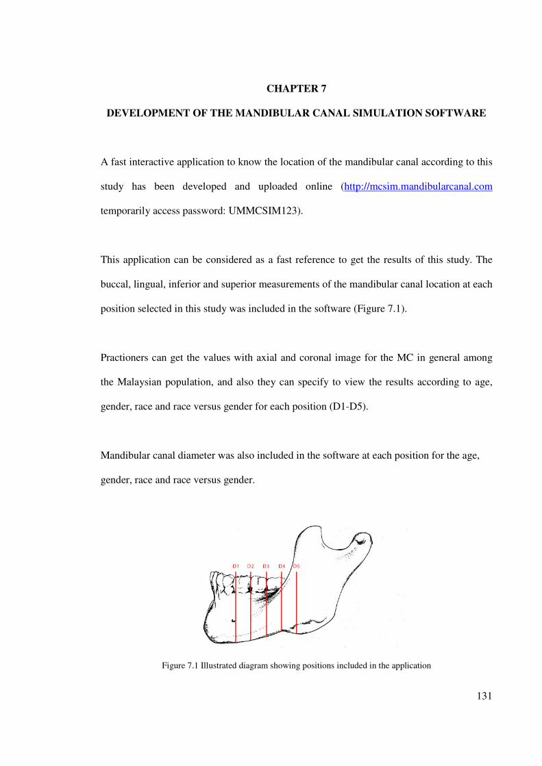
131
CHAPTER 7
DEVELOPMENT OF THE MANDIBULAR CANAL SIMULATION SOFTWARE
A fast interactive application to know the location of the mandibular canal according to this
study has been developed and uploaded online (http://mcsim.mandibularcanal.com
temporarily access password: UMMCSIM123).
This application can be considered as a fast reference to get the results of this study. The
buccal, lingual, inferior and superior measurements of the mandibular canal location at each
position selected in this study was included in the software (Figure 7.1).
Practioners can get the values with axial and coronal image for the MC in general among
the Malaysian population, and also they can specify to view the results according to age,
gender, race and race versus gender for each position (D1-D5).
Mandibular canal diameter was also included in the software at each position for the age,
gender, race and race versus gender.
Figure 7.1 Illustrated diagram showing positions included in the application
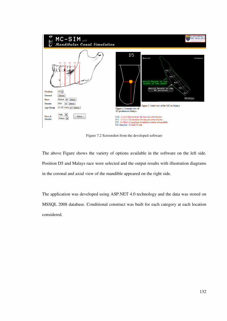
132
Figure 7.2 Screenshot from the developed software
The above Figure shows the variety of options available in the software on the left side.
Position D5 and Malays race were selected and the output results with illustration diagrams
in the coronal and axial view of the mandible appeared on the right side.
The application was developed using ASP.NET 4.0 technology and the data was stored on
MSSQL 2008 database. Conditional construct was built for each category at each location
considered.
133
REFERENCES
ALDSKOGIUS, H., ARVIDSSON, J. & GRANT, G. (1985) The reaction of primary
sensory neurons to peripheral nerve injury with particular emphasis on
transganglionic changes. Brain Res, 357, 27-46.
ALHASSANI, A. A. & ALGHAMDI, A. S. (2010) Inferior alveolar nerve injury in implant
dentistry: diagnosis, causes, prevention, and management. J Oral Implantol, 36,
401-7.
ANDERSON, L. C., KOSINSKI, T. F. & MENTAG, P. J. (1991) A review of the
intraosseous course of the nerves of the mandible. J Oral Implantol, 17, 394-403.
ANGELOPOULOS, C., THOMAS, S. L., HECHLER, S., PARISSIS, N. & HLAVACEK,
M. (2008) Comparison between digital panoramic radiography and cone-beam
computed tomography for the identification of the mandibular canal as part of
presurgical dental implant assessment. J Oral Maxillofac Surg, 66, 2130-5.
BABA, R., UEDA, K. & OKABE, M. (2004) Using a flat-panel detector in high resolution
cone beam CT for dental imaging. Dentomaxillofac Radiol, 33, 285-90.
BARTLING, R., FREEMAN, K. & KRAUT, R. A. (1999) The incidence of altered
sensation of the mental nerve after mandibular implant placement. J Oral
Maxillofac Surg, 57, 1408-12.
BEIROWSKI, B., ADALBERT, R., WAGNER, D., GRUMME, D. S., ADDICKS, K.,
RIBCHESTER, R. R. & COLEMAN, M. P. (2005) The progressive nature of
Wallerian degeneration in wild-type and slow Wallerian degeneration (WldS)
nerves. BMC Neurosci, 6, 6.
BROOKS, S. L., BEASON, R. C., SARMENT, D. & SUKOVIC, P. (2004) Implant
imaging with the I-CAT® cone-beam CT-a progress report.
CARTER, R. B. & KEEN, E. N. (1971) The intramandibular course of the inferior alveolar
nerve. J Anat, 108, 433-40.
CLAEYS, V. & WACKENS, G. (2005) Bifid mandibular canal: literature review and case
report. Dentomaxillofac Radiol, 34, 55-8.
COHNEN, M., KEMPER, J., MOBES, O., PAWELZIK, J. & MODDER, U. (2002)
Radiation dose in dental radiology. Eur Radiol, 12, 634-7.
COTTON, T. P., GEISLER, T. M., HOLDEN, D. T., SCHWARTZ, S. A. & SCHINDLER,
W. G. (2007) Endodontic applications of cone-beam volumetric tomography. J
Endod, 33, 1121-32.
CREAN, S. J. & POWIS, A. (1999) Neurological complications of local anaesthetics in
dentistry. Dent Update, 26, 344-9.
134
DAO, T. T. & MELLOR, A. (1998) Sensory disturbances associated with implant surgery.
Int J Prosthodont, 11, 462-9.
DE ANDRADE, E., OTOMO-CORGEL, J., PUCHER, J., RANGANATH, K. A. & ST
GEORGE, N., JR. (2001) The intraosseous course of the mandibular incisive nerve
in the mandibular symphysis. Int J Periodontics Restorative Dent, 21, 591-7.
DENG, W., CHEN, S. L., ZHANG, Z. W., HUANG, D. Y., ZHANG, X. & LI, X. (2008)
High-resolution magnetic resonance imaging of the inferior alveolar nerve using 3-
dimensional magnetization-prepared rapid gradient-echo sequence at 3.0T. J Oral
Maxillofac Surg, 66, 2621-6.
DENIO, D., TORABINEJAD, M. & BAKLAND, L. K. (1992) Anatomical relationship of
the mandibular canal to its surrounding structures in mature mandibles. J Endod, 18,
161-5.
DULA, K., MINI, R., VAN DER STELT, P. F., LAMBRECHT, J. T., SCHNEEBERGER,
P. & BUSER, D. (1996) Hypothetical mortality risk associated with spiral
computed tomography of the maxilla and mandible. Eur J Oral Sci, 104, 503-10.
FANIBUNDA, K., WHITWORTH, J. & STEELE, J. (1998) The management of
thermomechanically compacted gutta percha extrusion in the inferior dental canal.
Br Dent J, 184, 330-2.
FANUSCU, M. I. & CHANG, T. L. (2004) Three-dimensional morphometric analysis of
human cadaver bone: microstructural data from maxilla and mandible. Clin Oral
Implants Res, 15, 213-8.
FOX, N. A. (1989) The position of the inferior dental canal and its relation to the
mandibular second molar. Br Dent J, 167, 19-21.
FREDERIKSEN, N. L. (1995) Diagnostic imaging in dental implantology. Oral Surg Oral
Med Oral Pathol Oral Radiol Endod, 80, 540-54.
GERSHENSON, A., NATHAN, H. & LUCHANSKY, E. (1986) Mental foramen and
mental nerve: changes with age. Acta Anat (Basel), 126, 21-8.
GIBBS, S. J. (2000) Effective dose equivalent and effective dose: comparison for common
projections in oral and maxillofacial radiology. Oral Surg Oral Med Oral Pathol
Oral Radiol Endod, 90, 538-45.
GIJBELS, F., DE MEYER, A. M., BOU SERHAL, C., VAN DEN BOSSCHE, C.,
DECLERCK, J., PERSOONS, M. & JACOBS, R. (2000) The subjective image
quality of direct digital and conventional panoramic radiography. Clin Oral
Investig, 4, 162-7.
GOSLING, J. A. (1985) Atlas of human anatomy with integrated text, Philadelphia
London ; New York, J.B. Lippincott Co. ;Gower Medical Pub.
135
GOWGIEL, J. M. (1992) The position and course of the mandibular canal. J Oral
Implantol, 18, 383-5.
GREENSTEIN, G., CAVALLARO, J. & TARNOW, D. (2008) Practical application of
anatomy for the dental implant surgeon. J Periodontol, 79, 1833-46.
GREENSTEIN, G. & TARNOW, D. (2006) The mental foramen and nerve: clinical and
anatomical factors related to dental implant placement: a literature review. J
Periodontol, 77, 1933-43.
GROVER, P. S. & LORTON, L. (1983) Bifid mandibular nerve as a possible cause of
inadequate anesthesia in the mandible. J Oral Maxillofac Surg, 41, 177-9.
GULTEKIN, S., ARAC, M., CELIK, H., KARAOSMAOGLU, A. D. & ISIK, S. (2003)
[Assessment of mandibular vascular canals by dental CT]. Tani Girisim Radyol, 9,
188-91.
HAAS, D. A. & LENNON, D. (1995) A 21 year retrospective study of reports of
paresthesia following local anesthetic administration. J Can Dent Assoc, 61, 319-20,
323-6, 329-30.
HALLIKAINEN, D., IIZUKA, T. & LINDQVIST, C. (1992) Cross-sectional tomography
in evaluation of patients undergoing sagittal split osteotomy. J Oral Maxillofac
Surg, 50, 1269-73.
HAMADA, Y., KONDOH, T., NOGUCHI, K., IINO, M., ISONO, H., ISHII, H.,
MISHIMA, A., KOBAYASHI, K. & SETO, K. (2005) Application of limited cone
beam computed tomography to clinical assessment of alveolar bone grafting: a
preliminary report. Cleft Palate Craniofac J, 42, 128-37.
HARN, S. D. & DURHAM, T. M. (1990) Incidence of lingual nerve trauma and
postinjection complications in conventional mandibular block anesthesia. J Am Dent
Assoc, 121, 519-23.
HASKELL, B., DAY, M. & TETZ, J. (1986) Computer-aided modeling in the assessment
of the biomechanical determinants of diverse skeletal patterns. Am J Orthod, 89,
363-82.
HATCHER, D. C., DIAL, C. & MAYORGA, C. (2003) Cone beam CT for pre-surgical
assessment of implant sites. J Calif Dent Assoc, 31, 825-33.
HEASMAN, P. A. (1988) Variation in the position of the inferior dental canal and its
significance to restorative dentistry. J Dent, 16, 36-9.
HILLERUP, S. & JENSEN, R. (2006) Nerve injury caused by mandibular block analgesia.
Int J Oral Maxillofac Surg, 35, 437-43.
IKEDA, K., HO, K. C., NOWICKI, B. H. & HAUGHTON, V. M. (1996) Multiplanar MR
and anatomic study of the mandibular canal. AJNR Am J Neuroradiol, 17, 579-84.
136
JACOBS, R., ADRIANSENS, A., NAERT, I., QUIRYNEN, M., HERMANS, R. & VAN
STEENBERGHE, D. (1999) Predictability of reformatted computed tomography
for pre-operative planning of endosseous implants. Dentomaxillofac Radiol, 28, 37-
41.
JACOBS, R., MRAIWA, N., VAN STEENBERGHE, D., SANDERINK, G. &
QUIRYNEN, M. (2004) Appearance of the mandibular incisive canal on panoramic
radiographs. Surg Radiol Anat, 26, 329-33.
JONES, D. L. & THRASH, W. J. (1992) Electrophysiological assessment of human
inferior alveolar nerve function. J Oral Maxillofac Surg, 50, 581-5.
JUODZBALYS, G. & WANG, H.-L. (2010) Guidelines for the Identification of the
Mandibular Vital Structures: Practical Clinical Applications of Anatomy and
Radiological Examination Methods. Journal of Oral & Maxillofacial Research, 1,
e1.
JUODZBALYS, G., WANG, H.-L. & SABALYS, G. (2011) Injury of the Inferior Alveolar
Nerve during Implant Placement: a Literature Review. JOURNAL OF ORAL &
MAXILLOFACIAL RESEARCH 2.
KAMBUROGLU, K., KILIC, C., OZEN, T. & YUKSEL, S. P. (2009) Measurements of
mandibular canal region obtained by cone-beam computed tomography: a cadaveric
study. Oral Surg Oral Med Oral Pathol Oral Radiol Endod, 107, e34-42.
KARABOUTA-VOULGAROPOULOU, I. & MARTIS, C. (1984) Facial paresis following
sagittal split osteotomy. Report of two cases. Oral Surg Oral Med Oral Pathol, 57,
600-3.
KHAWAJA, N. & RENTON, T. (2009) Case studies on implant removal influencing the
resolution of inferior alveolar nerve injury. Br Dent J, 206, 365-70.
KIESER, J., KIESER, D. & HAUMAN, T. (2005) The course and distribution of the
inferior alveolar nerve in the edentulous mandible. J Craniofac Surg, 16, 6-9.
KIESER, J. A., PAULIN, M. & LAW, B. (2004) Intrabony course of the inferior alveolar
nerve in the edentulous mandible. Clin Anat, 17, 107-11.
KIM, I. S., KIM, S. G., KIM, Y. K. & KIM, J. D. (2006) Position of the mental foramen in
a Korean population: a clinical and radiographic study. Implant Dent, 15, 404-11.
KIPP, D. P., GOLDSTEIN, B. H. & WEISS, W. W., JR. (1980) Dysesthesia after
mandibular third molar surgery: a retrospective study and analysis of 1,377 surgical
procedures. J Am Dent Assoc, 100, 185-92.
KLINGE, B., PETERSSON, A. & MALY, P. (1989) Location of the mandibular canal:
comparison of macroscopic findings, conventional radiography, and computed
tomography. Int J Oral Maxillofac Implants, 4, 327-32.
137
KOBAYASHI, K., SHIMODA, S., NAKAGAWA, Y. & YAMAMOTO, A. (2004)
Accuracy in measurement of distance using limited cone-beam computerized
tomography. Int J Oral Maxillofac Implants, 19, 228-31.
KOMAKI, R., WADLER, S., PETERS, T., BYHARDT, R. W., ORDER, S.,
GALLAGHER, M. J., HERSKOVIC, A. & PEDERSON, J. (1992) High-dose local
irradiation plus prophylactic hepatic irradiation and chemotherapy for inoperable
adenocarcinoma of the pancreas. A preliminary report of a multi-institutional trial
(Radiation Therapy Oncology Group Protocol 8801). Cancer, 69, 2807-12.
KRAUT, R. A. & CHAHAL, O. (2002) Management of patients with trigeminal nerve
injuries after mandibular implant placement. J Am Dent Assoc, 133, 1351-4.
LAM, D. E. (2007) Where does cone beam computed tomography fit into modern
dental practice? J.C.D.A., 73, 921-923.
LAMAS PELAYO, J., PENARROCHA DIAGO, M. & MARTI BOWEN, E. (2008)
Intraoperative complications during oral implantology. Med Oral Patol Oral Cir
Bucal, 13, E239-43.
LANGLAIS, R. P., BROADUS, R. & GLASS, B. J. (1985) Bifid mandibular canals in
panoramic radiographs. J Am Dent Assoc, 110, 923-6.
LASCALA, C. A., PANELLA, J. & MARQUES, M. M. (2004) Analysis of the accuracy of
linear measurements obtained by cone beam computed tomography (CBCT-
NewTom). Dentomaxillofac Radiol, 33, 291-4.
LAVELLE, C. L. (1985) Preliminary study of mandibular shape after tooth loss. J Prosthet
Dent, 53, 726-30.
LECKEL, M., KRESS, B. & SCHMITTER, M. (2009) Neuropathic pain resulting from
implant placement: case report and diagnostic conclusions. J Oral Rehabil, 36, 543-
6.
LEVINE, M. H., GODDARD, A. L. & DODSON, T. B. (2007) Inferior alveolar nerve
canal position: a clinical and radiographic study. J Oral Maxillofac Surg, 65, 470-4.
LINDH, C. & PETERSSON, A. (1989) Radiologic examination for location of the
mandibular canal: a comparison between panoramic radiography and conventional
tomography. Int J Oral Maxillofac Implants, 4, 249-53.
LINDH, C., PETERSSON, A. & KLINGE, B. (1992) Visualisation of the mandibular canal
by different radiographic techniques. Clin Oral Implants Res, 3, 90-7.
LINDH, C., PETERSSON, A. & KLINGE, B. (1995) Measurements of distances related to
the mandibular canal in radiographs. Clin Oral Implants Res, 6, 96-103.
138
LINDQUIST, C. C. & OBEID, G. (1988) Complications of genioplasty done alone or in
combination with sagittal split-ramus osteotomy. Oral Surg Oral Med Oral Pathol,
66, 13-6.
LITTNER, M. M., KAFFE, I., TAMSE, A. & DICAPUA, P. (1986) Relationship between
the apices of the lower molars and mandibular canal--a radiographic study. Oral
Surg Oral Med Oral Pathol, 62, 595-602.
LUDLOW, J. B., DAVIES-LUDLOW, L. E. & BROOKS, S. L. (2003) Dosimetry of two
extraoral direct digital imaging devices: NewTom cone beam CT and Orthophos
Plus DS panoramic unit. Dentomaxillofac Radiol, 32, 229-34.
LUDLOW, J. B., DAVIES-LUDLOW, L. E., BROOKS, S. L. & HOWERTON, W. B.
(2006) Dosimetry of 3 CBCT devices for oral and maxillofacial radiology: CB
Mercuray, NewTom 3G and i-CAT. Dentomaxillofac Radiol, 35, 219-26.
MACDONALD-JANKOWSKI, T. S. & ORPE, E. C. (2007) Some Current Legal Issues
that May Affect Oral and Maxillofacial Radiology Part 2: Digital Monitors and
Cone-Beam Computed Tomography. J.C.D.A., 73.
MAH, J. K., DANFORTH, R. A., BUMANN, A. & HATCHER, D. (2003) Radiation
absorbed in maxillofacial imaging with a new dental computed tomography device.
Oral Surg Oral Med Oral Pathol Oral Radiol Endod, 96, 508-13.
MAKI, K., INOU, N., TAKANISHI, A. & MILLER, A. J. (2003) Computer-assisted
simulations in orthodontic diagnosis and the application of a new cone beam X-ray
computed tomography. Orthod Craniofac Res, 6 Suppl 1, 95-101; discussion 179-
82.
MALAMED, S. F. (2010) Local anesthesia reversal. Dent Today, 29, 65-6, 68, 71-2
passim; quiz 74.
MARDINGER, O., CHAUSHU, G., ARENSBURG, B., TAICHER, S. & KAFFE, I.
(2000) Anterior loop of the mental canal: an anatomical-radiologic study. Implant
Dent, 9, 120-5.
MARDINI, S. & GOHEL, A. (2008) Exploring the Mandibular Canal in 3 Dimensions.An
Overview of Frequently Encountered.Variations in Canal Anatomy. AADMRT.
MERCIER, P. (1973) The inner osseous architecture and the sagittal splitting of the
ascending ramus of the mandible. J Maxillofac Surg, 1, 171-6.
MILLER, C. S., NUMMIKOSKI, P. V., BARNETT, D. A. & LANGLAIS, R. P. (1990)
Cross-sectional tomography. A diagnostic technique for determining the
buccolingual relationship of impacted mandibular third molars and the inferior
alveolar neurovascular bundle. Oral Surg Oral Med Oral Pathol, 70, 791-7.
MISCH, C. (1999) Bone density: A key determinant for clinical success St Louis CV
Mosby Company
139
MRAIWA, N., JACOBS, R., MOERMAN, P., LAMBRICHTS, I., VAN STEENBERGHE,
D. & QUIRYNEN, M. (2003) Presence and course of the incisive canal in the
human mandibular interforaminal region: two-dimensional imaging versus
anatomical observations. Surg Radiol Anat, 25, 416-23.
NAITOH, M., HIRAIWA, Y., AIMIYA, H. & ARIJI, E. (2009a) Observation of bifid
mandibular canal using cone-beam computerized tomography. Int J Oral Maxillofac
Implants, 24, 155-9.
NAITOH, M., HIRUKAWA, A., KATSUMATA, A. & ARIJI, E. (2009b) Evaluation of
voxel values in mandibular cancellous bone: relationship between cone-beam
computed tomography and multislice helical computed tomography. Clin Oral
Implants Res, 20, 503-6.
NAITOH, M., KATSUMATA, A., HIRAIWA, Y., AIMIYA, H., OHSAKI, C. & ARIJI, E.
(2008) Can mandibular depiction be improved by changing the thickness of double-
oblique computed tomography images? Implant Dent, 17, 271-7.
NAKAGAWA, Y., KOBAYASHI, K., ISHII, H., MISHIMA, A., ASADA, K. &
ISHIBASHI, K. (2002) Preoperative application of limited cone beam computerized
tomography as an assessment tool before minor oral surgery. Int J Oral Maxillofac
Surg, 31, 322-6.
NARAYANA, K. & VASUDHA, S. (2004) Intraosseous course of the inferior alveolar
(dental) nerve and its relative position in the mandible. Indian J Dent Res, 15, 99-
102.
NAZARIAN, Y., ELIAV, E. & NAHLIELI, O. (2003) [Nerve injury following implant
placement: prevention, diagnosis and treatment modalities]. Refuat Hapeh
Vehashinayim, 20, 44-50, 101.
NEUGEBAUER, J., SHIRANI, R., MISCHKOWSKI, R. A., RITTER, L., SCHEER, M.,
KEEVE, E. & ZOLLER, J. E. (2008) Comparison of cone-beam volumetric
imaging and combined plain radiographs for localization of the mandibular canal
before removal of impacted lower third molars. Oral Surg Oral Med Oral Pathol
Oral Radiol Endod, 105, 633-42; discussion 643.
NGAN, D. C., KHARBANDA, O. P., GEENTY, J. P. & DARENDELILER, M. A. (2003)
Comparison of radiation levels from computed tomography and conventional dental
radiographs. Aust Orthod J, 19, 67-75.
NICKEL, A. A., JR. (1990) A retrospective study of paresthesia of the dental alveolar
nerves. Anesth Prog, 37, 42-5.
NORTJĔ, C. J., FARMAN, A. G. & DE, V. J. J. J. (1977a) The radiographic appearance of
the inferior dental canal: an additional variation. Br J Oral Surg, 15, 171-2.
NORTJĔ, C. J., FARMAN, A. G. & GROTEPASS, F. W. (1977b) Variations in the normal
anatomy of the inferior dental (mandibular) canal: a retrospective study of
140
panoramic radiographs from 3612 routine dental patients. Br J Oral Surg, 15, 55-
63.
NORTON, M. R. & GAMBLE, C. (2001) Bone classification: an objective scale of bone
density using the computerized tomography scan. Clin Oral Implants Res, 12, 79-
84.
OBRADOVIC, O., TODOROVIC, L., PESIC, V., PEJKOVIC, B. & VITANOVIC, V.
(1993) Morphometric analysis of mandibular canal: clinical aspects. Bull Group Int
Rech Sci Stomatol Odontol, 36, 109-13.
OBRADOVIC, O., TODOROVIC, L. & VITANOVIC, V. (1995) Anatomical
considerations relevant to implant procedures in the mandible. Bull Group Int Rech
Sci Stomatol Odontol, 38, 39-44.
OGAWA, T., ENCISO, R., MEMON, A., MAH, J. K. & CLARK, G. T. (2005) Evaluation
of 3D airway imaging of obstructive sleep apnea with cone-beam computed
tomography. Stud Health Technol Inform, 111, 365-8.
PEKER, I., ALKURT, M. T. & MICHCIOGLU, T. (2008) The use of 3 different imaging
methods for the localization of the mandibular canal in dental implant planning. Int
J Oral Maxillofac Implants, 23, 463-70.
POGREL, M. A. & KABAN, L. B. (1993) Injuries to the inferior alveolar and lingual
nerves. J Calif Dent Assoc, 21, 50-4.
POGREL, M. A. & MAGHEN, A. (2001) The use of autogenous vein grafts for inferior
alveolar and lingual nerve reconstruction. J Oral Maxillofac Surg, 59, 985-8;
discussion 988-93.
POLLAND, K. E., MUNRO, S., REFORD, G., LOCKHART, A., LOGAN, G.,
BROCKLEBANK, L. & MCDONALD, S. W. (2001) The mandibular canal of the
edentulous jaw. Clin Anat, 14, 445-52.
RAJCHEL, J., ELLIS, E., 3RD & FONSECA, R. J. (1986) The anatomical location of the
mandibular canal: its relationship to the sagittal ramus osteotomy. Int J Adult
Orthodon Orthognath Surg, 1, 37-47.
RIGOLONE, M., PASQUALINI, D., BIANCHI, L., BERUTTI, E. & BIANCHI, S. D.
(2003) Vestibular surgical access to the palatine root of the superior first molar:
"low-dose cone-beam" CT analysis of the pathway and its anatomic variations. J
Endod, 29, 773-5.
ROTHMAN, S. L., CHAFTEZ, N., RHODES, M. L. & SCHWARZ, M. S. (1988) CT in
the preoperative assessment of the mandible and maxilla for endosseous implant
surgery. Work in progress. Radiology, 168, 171-5.
141
ROUAS, P., NANCY, J. & BAR, D. (2007) Identification of double mandibular canals:
literature review and three case reports with CT scans and cone beam CT.
Dentomaxillofac Radiol, 36, 34-8.
RUEDA, S., GIL, J. A., PICHERY, R. & ALCANIZ, M. (2006) Automatic segmentation
of jaw tissues in CT using active appearance models and semi-automatic
landmarking. Med Image Comput Comput Assist Interv, 9, 167-74.
SANCHIS, J. M., PENARROCHA, M. & SOLER, F. (2003) Bifid mandibular canal. J
Oral Maxillofac Surg, 61, 422-4.
SATO, I., UENO, R., KAWAI, T. & YOSUE, T. (2005) Rare courses of the mandibular
canal in the molar regions of the human mandible: a cadaveric study. Okajimas
Folia Anat Jpn, 82, 95-101.
SATO, S., ARAI, Y., SHINODA, K. & ITO, K. (2004) Clinical application of a new cone-
beam computerized tomography system to assess multiple two-dimensional images
for the preoperative treatment planning of maxillary implants: case reports.
Quintessence Int, 35, 525-8.
SCAF, G., LURIE, A. G., MOSIER, K. M., KANTOR, M. L., RAMSBY, G. R. &
FREEDMAN, M. L. (1997) Dosimetry and cost of imaging osseointegrated
implants with film-based and computed tomography. Oral Surg Oral Med Oral
Pathol Oral Radiol Endod, 83, 41-8.
SCARFE, W. C., FARMAN, A. G. & SUKOVIC, P. (2006) Clinical Applications of Cone-
Beam Computed Tomography in Dental Practice. JCDA, 72.
SCHRAMM, A., RU¨CKER, M., SAKKAS, N., SCHO¨NB, R., DU¨ KERB, J. &
GELLRICH, N. C. (2005) The use of cone beam CT in cranio-maxillofacial
surgery. International Congress Series, 1281, 1200-1204.
SCHULZE, D., HEILAND, M., THURMANN, H. & ADAM, G. (2004) Radiation
exposure during midfacial imaging using 4- and 16-slice computed tomography,
cone beam computed tomography systems and conventional radiography.
Dentomaxillofac Radiol, 33, 83-6.
SMILER, D. G. (1993) Repositioning the inferior alveolar nerve for placement of
endosseous implants: technical note. Int J Oral Maxillofac Implants, 8, 145-50.
SONIC, M., ABRAHAMS, J. & FAIELLA, R. (1994) A comparison of the accuracy of
periapical, panoramic, and computerized tomographic radiographs in locating the
mandibular canal. Int J Oral Maxillofac Implants
9, 455-460
STACY, G. C. & HAJJAR, G. (1994) Barbed needle and inexplicable paresthesias and
trismus after dental regional anesthesia. Oral Surg Oral Med Oral Pathol, 77, 585-
8.
142
SUKOVIC, P. (2003) Cone beam computed tomography in craniofacial imaging. Orthod
Craniofac Res, 6 Suppl 1, 31-6; discussion 179-82.
TAL, H. & MOSES, O. (1991) A comparison of panoramic radiography with computed
tomography in the planning of implant surgery. Dentomaxillofac Radiol, 20, 40-2.
TAMAS, F. (1987) Position of the mandibular canal. Int J Oral Maxillofac Surg, 16, 65-9.
TAMMISALO, T., HAPPONEN, R. P. & TAMMISALO, E. H. (1992) Stereographic
assessment of mandibular canal in relation to the roots of impacted lower third
molar using multiprojection narrow beam radiography. Int J Oral Maxillofac Surg,
21, 85-9.
TANTANAPORNKUL, W., OKOUCHI, K., FUJIWARA, Y., YAMASHIRO, M.,
MARUOKA, Y., OHBAYASHI, N. & KURABAYASHI, T. (2007) A comparative
study of cone-beam computed tomography and conventional panoramic radiography
in assessing the topographic relationship between the mandibular canal and
impacted third molars. Oral Surg Oral Med Oral Pathol Oral Radiol Endod, 103,
253-9.
TAY, A. B. & ZUNIGA, J. R. (2007) Clinical characteristics of trigeminal nerve injury
referrals to a university centre. Int J Oral Maxillofac Surg, 36, 922-7.
TEHEMAR, S. H. (1999) Factors affecting heat generation during implant site preparation:
a review of biologic observations and future considerations. Int J Oral Maxillofac
Implants, 14, 127-36.
THEISEN, F. C., SHULTZ, R. E. & ELLEDGE, D. A. (1990) Displacement of a root form
implant into the mandibular canal. Oral Surg Oral Med Oral Pathol, 70, 24-8.
TSIKLAKIS, K., SYRIOPOULOS, K. & STAMATAKIS, H. C. (2004) Radiographic
examination of the temporomandibular joint using cone beam computed
tomography. Dentomaxillofac Radiol, 33, 196-201.
ULM, C. W., SOLAR, P., BLAHOUT, R., MATEJKA, M., WATZEK, G. & GRUBER, H.
(1993) Location of the mandibular canal within the atrophic mandible. Br J Oral
Maxillofac Surg, 31, 370-5.
VAN DER STELT, P. F. (2005) Filmless imaging: the uses of digital radiography in dental
practice. J Am Dent Assoc, 136, 1379-87.
VAN MERKESTEYN, J. P., GROOT, R. H., VAN LEEUWAARDEN, R. & KROON, F.
H. (1987) Intra-operative complications in sagittal and vertical ramus osteotomies.
Int J Oral Maxillofac Surg, 16, 665-70.
VAZQUEZ, L., SAULACIC, N., BELSER, U. & BERNARD, J. P. (2008) Efficacy of
panoramic radiographs in the preoperative planning of posterior mandibular
implants: a prospective clinical study of 1527 consecutively treated patients. Clin
Oral Implants Res, 19, 81-5.
143
VENTA, I., LINDQVIST, C. & YLIPAAVALNIEMI, P. (1998) Malpractice claims for
permanent nerve injuries related to third molar removals. Acta Odontol Scand, 56,
193-6.
WADU, S. G., PENHALL, B. & TOWNSEND, G. C. (1997) Morphological variability of
the human inferior alveolar nerve. Clin Anat, 10, 82-7.
WANG, J. C., GUI, L., ZHANG, Z. Y., NIU, F. & CAI, J. L. (2008) Significance of
location of mandibular canal by 3-dimensional CT in the mandibular angle
osteotomy. Zhonghua Zheng Xing Wai Ke Za Zhi, 24, 360-2.
WATANABE, H., MOHAMMAD ABDUL, M., KURABAYASHI, T. & AOKI, H. (2009)
Mandible size and morphology determined with CT on a premise of dental implant
operation. Surg Radiol Anat, 32, 343-9.
WHITE, S. C., HESLOP, E. W., HOLLENDER, L. G., MOSIER, K. M., RUPRECHT, A.
& SHROUT, M. K. (2001) Parameters of radiologic care: An official report of the
American Academy of Oral and Maxillofacial Radiology. Oral Surg Oral Med Oral
Pathol Oral Radiol Endod, 91, 498-511.
WHITE, S. C. & PHAROAH, M. J. (2009) Oral radiology : principles and interpretation,
St. Louis, Mo., Mosby/Elsevier.
WILLIAMS, P., WARWICK, R., DYSON, M. & BANNISTER, L. (1989) Gray's anatomy,
Edinburg; London; Melbourne, Churchill Livingstone.
WISMEIJER, D., VAN WAAS, M. A., VERMEEREN, J. I. & KALK, W. (1997) Patients'
perception of sensory disturbances of the mental nerve before and after implant
surgery: a prospective study of 110 patients. Br J Oral Maxillofac Surg, 35, 254-9.
WORTHINGTON, P. (1995) Medicolegal aspects of oral implant surgery. Aust
Prosthodont J, 9 Suppl, 13-7.
WORTHINGTON, P. (2004) Injury to the inferior alveolar nerve during implant
placement: a formula for protection of the patient and clinician. Int J Oral
Maxillofac Implants, 19, 731-4.
YAJIMA, A., OTONARI-YAMAMOTO, M., SANO, T., HAYAKAWA, Y., OTONARI,
T., TANABE, K., WAKOH, M., MIZUTA, S., YONEZU, H., NAKAGAWA, K. &
YAJIMA, Y. (2006) Cone-beam CT (CB Throne) applied to dentomaxillofacial
region. Bull Tokyo Dent Coll, 47, 133-41.
YANG, J., CAVALCANTI, M. G., RUPRECHT, A. & VANNIER, M. W. (1999) 2-D and
3-D reconstructions of spiral computed tomography in localization of the inferior
alveolar canal for dental implants. Oral Surg Oral Med Oral Pathol Oral Radiol
Endod, 87, 369-74.
144
YLIKONTIOLA, L., KINNUNEN, J. & OIKARINEN, K. (2000) Factors affecting
neurosensory disturbance after mandibular bilateral sagittal split osteotomy. J Oral
Maxillofac Surg, 58, 1234-9; discussion 1239-40.
YLIKONTIOLA, L., MOBERG, K., HUUMONEN, S., SOIKKONEN, K. &
OIKARINEN, K. (2002) Comparison of three radiographic methods used to locate
the mandibular canal in the buccolingual direction before bilateral sagittal split
osteotomy. Oral Surg Oral Med Oral Pathol Oral Radiol Endod, 93, 736-42.
ZICCARDI, V. B. & ASSAEL, L. A. (2001) Mechanisms of trigeminal nerve injuries.
Atlas Oral Maxillofac Surg Clin North Am, 9, 1-11.
ZIEGLER, C. M., WOERTCHE, R., BRIEF, J. & HASSFELD, S. (2002) Clinical
indications for digital volume tomography in oral and maxillofacial surgery.
Dentomaxillofac Radiol, 31, 126-30.
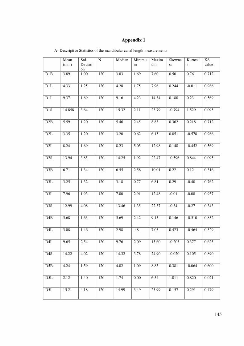
145
Appendix 1
A- Descriptive Statistics of the mandibular canal length measurements
Mean
(mm)
Std.
Deviati
on
N Median Minimu
m
Maxim
um
Skewne
ss
Kurtosi
s
KS
value
D1B 3.89 1.00 120 3.83 1.69 7.60 0.50 0.76 0.712
D1L 4.33 1.25 120 4.28 1.75 7.96 0.244 -0.011 0.986
D1I 9.37 1.69 120 9.16 4.23 14.34 0.180 0.23 0.569
D1S 14.858 3.64 120 15.32 2.11 23.79 -0.794 1.529 0.095
D2B 5.59 1.20 120 5.46 2.45 8.83 0.362 0.218 0.712
D2L 3.35 1.20 120 3.20 0.62 6.15 0.051 -0.578 0.986
D2I 8.24 1.69 120 8.23 5.05 12.98 0.148 -0.452 0.569
D2S 13.94 3.85 120 14.25 1.92 22.47 -0.596 0.844 0.095
D3B 6.71 1.34 120 6.55 2.58 10.01 0.22 0.12 0.316
D3L 3.25 1.32 120 3.18 0.77 6.81 0.29 -0.40 0.762
D3I 7.96 1.93 120 7.80 2.91 12.48 -0.01 -0.08 0.937
D3S 12.99 4.08 120 13.46 1.35 22.37 -0.34 -0.27 0.343
D4B 5.68 1.63 120 5.69 2.42 9.15 0.146 -0.510 0.832
D4L 3.08 1.46 120 2.98 .48 7.03 0.423 -0.464 0.329
D4I 9.65 2.54 120 9.76 2.09 15.60 -0.203 0.377 0.625
D4S 14.22 4.02 120 14.32 3.78 24.90 -0.020 0.105 0.890
D5B 4.24 1.59 120 4.02 1.09 8.83 0.381 -0.064 0.600
D5L 2.12 1.40 120 1.74 0.00 6.54 1.011 0.820 0.021
D5I 15.21 4.18 120 14.99 3.49 25.99 0.157 0.291 0.479
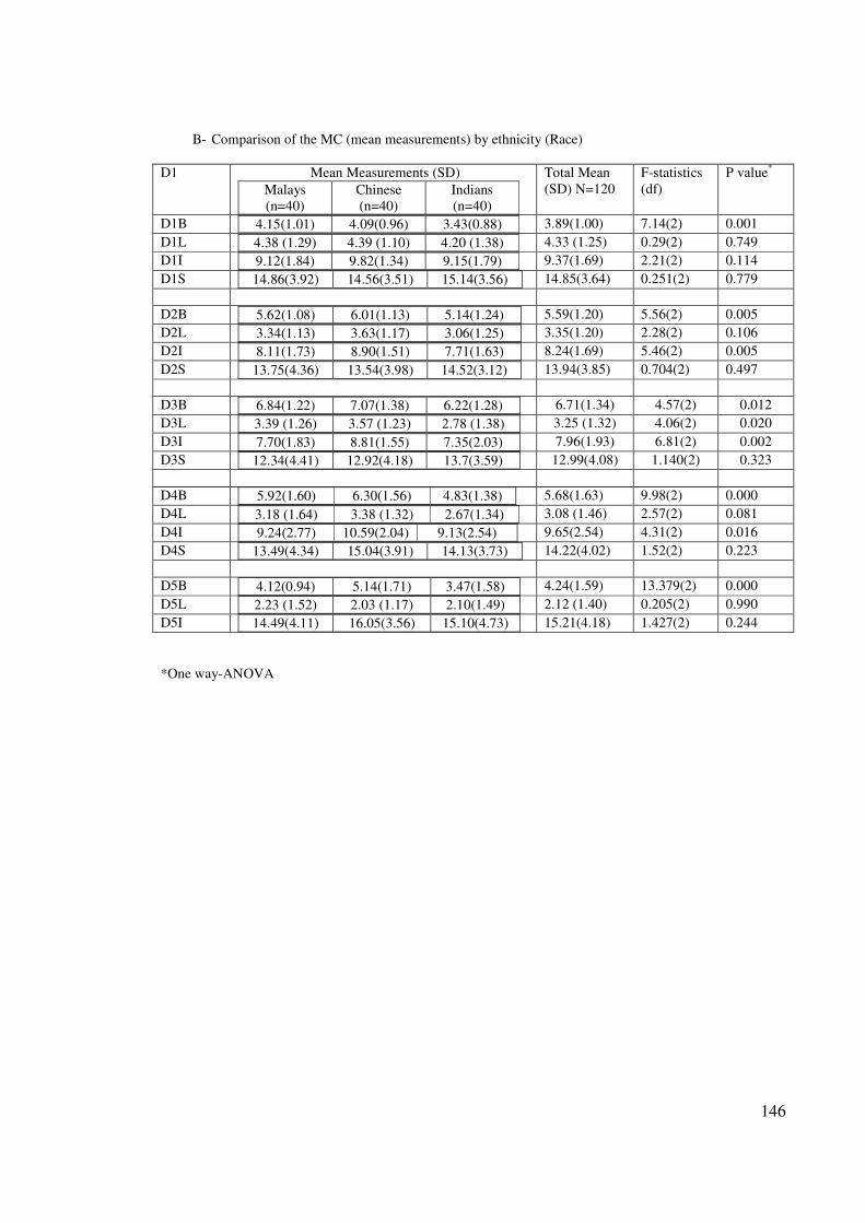
146
B- Comparison of the MC (mean measurements) by ethnicity (Race)
D1
Mean Measurements (SD)
Malays
(n=40)
Chinese
(n=40)
Indians
(n=40)
Total Mean
(SD) N=120
F-statistics
(df)
P value*
D1B 4.15(1.01) 4.09(0.96) 3.43(0.88)
3.89(1.00) 7.14(2) 0.001
D1L 4.38 (1.29) 4.39 (1.10) 4.20 (1.38)
4.33 (1.25) 0.29(2) 0.749
D1I 9.12(1.84) 9.82(1.34) 9.15(1.79)
9.37(1.69) 2.21(2) 0.114
D1S 14.86(3.92) 14.56(3.51) 15.14(3.56)
14.85(3.64) 0.251(2) 0.779
D2B 5.62(1.08) 6.01(1.13) 5.14(1.24)
5.59(1.20) 5.56(2) 0.005
D2L 3.34(1.13) 3.63(1.17) 3.06(1.25)
3.35(1.20) 2.28(2) 0.106
D2I 8.11(1.73) 8.90(1.51) 7.71(1.63)
8.24(1.69) 5.46(2) 0.005
D2S 13.75(4.36) 13.54(3.98) 14.52(3.12)
13.94(3.85) 0.704(2) 0.497
D3B 6.84(1.22) 7.07(1.38) 6.22(1.28)
6.71(1.34) 4.57(2) 0.012
D3L 3.39 (1.26) 3.57 (1.23) 2.78 (1.38)
3.25 (1.32) 4.06(2) 0.020
D3I 7.70(1.83) 8.81(1.55) 7.35(2.03)
7.96(1.93) 6.81(2) 0.002
D3S 12.34(4.41) 12.92(4.18) 13.7(3.59)
12.99(4.08) 1.140(2) 0.323
D4B 5.92(1.60) 6.30(1.56) 4.83(1.38)
5.68(1.63) 9.98(2) 0.000
D4L 3.18 (1.64) 3.38 (1.32) 2.67(1.34)
3.08 (1.46) 2.57(2) 0.081
D4I 9.24(2.77) 10.59(2.04) 9.13(2.54)
9.65(2.54) 4.31(2) 0.016
D4S 13.49(4.34) 15.04(3.91) 14.13(3.73)
14.22(4.02) 1.52(2) 0.223
D5B 4.12(0.94) 5.14(1.71) 3.47(1.58)
4.24(1.59) 13.379(2) 0.000
D5L 2.23 (1.52) 2.03 (1.17) 2.10(1.49)
2.12 (1.40) 0.205(2) 0.990
D5I 14.49(4.11) 16.05(3.56) 15.10(4.73)
15.21(4.18) 1.427(2) 0.244
*One way-ANOVA
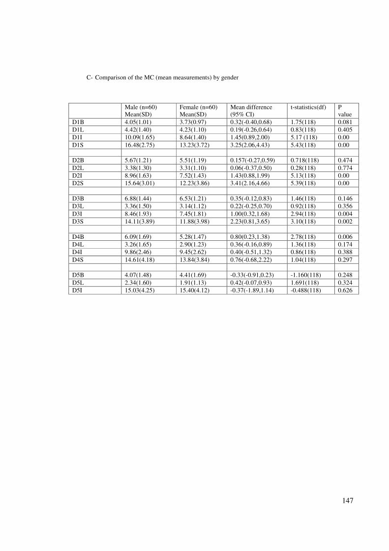
147
C- Comparison of the MC (mean measurements) by gender
Male (n=60)
Mean(SD)
Female (n=60)
Mean(SD)
Mean difference
(95% CI)
t-statistics(df) P
value
D1B 4.05(1.01) 3.73(0.97) 0.32(-0.40,0.68) 1.75(118) 0.081
D1L 4.42(1.40) 4.23(1.10) 0.19(-0.26,0.64) 0.83(118) 0.405
D1I 10.09(1.65) 8.64(1.40) 1.45(0.89,2.00) 5.17 (118) 0.00
D1S 16.48(2.75) 13.23(3.72) 3.25(2.06,4.43) 5.43(118) 0.00
D2B 5.67(1.21) 5.51(1.19) 0.157(-0.27,0.59) 0.718(118) 0.474
D2L 3.38(1.30) 3.31(1.10) 0.06(-0.37,0.50) 0.28(118) 0.774
D2I 8.96(1.63) 7.52(1.43) 1.43(0.88,1.99) 5.13(118) 0.00
D2S 15.64(3.01) 12.23(3.86) 3.41(2.16,4.66) 5.39(118) 0.00
D3B 6.88(1.44) 6.53(1.21) 0.35(-0.12,0.83) 1.46(118) 0.146
D3L 3.36(1.50) 3.14(1.12) 0.22(-0.25,0.70) 0.92(118) 0.356
D3I 8.46(1.93) 7.45(1.81) 1.00(0.32,1.68) 2.94(118) 0.004
D3S 14.11(3.89) 11.88(3.98) 2.23(0.81,3.65) 3.10(118) 0.002
D4B 6.09(1.69) 5.28(1.47) 0.80(0.23,1.38) 2.78(118) 0.006
D4L 3.26(1.65) 2.90(1.23) 0.36(-0.16,0.89) 1.36(118) 0.174
D4I 9.86(2.46) 9.45(2.62) 0.40(-0.51,1.32) 0.86(118) 0.388
D4S 14.61(4.18) 13.84(3.84) 0.76(-0.68,2.22) 1.04(118) 0.297
D5B 4.07(1.48) 4.41(1.69) -0.33(-0.91,0.23) -1.160(118) 0.248
D5L 2.34(1.60) 1.91(1.13) 0.42(-0.07,0.93) 1.691(118) 0.324
D5I 15.03(4.25) 15.40(4.12) -0.37(-1.89,1.14) -0.488(118) 0.626
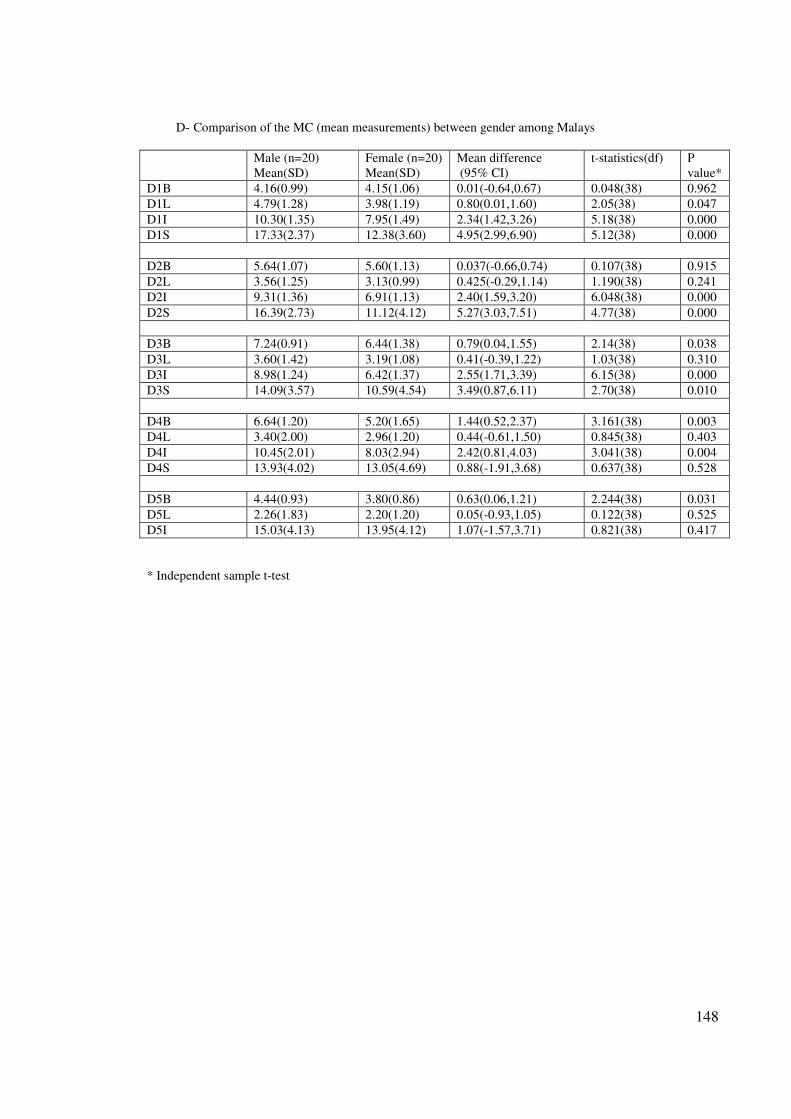
148
D- Comparison of the MC (mean measurements) between gender among Malays
Male (n=20)
Mean(SD)
Female (n=20)
Mean(SD)
Mean difference
(95% CI)
t-statistics(df) P
value*
D1B 4.16(0.99) 4.15(1.06) 0.01(-0.64,0.67) 0.048(38) 0.962
D1L 4.79(1.28) 3.98(1.19) 0.80(0.01,1.60) 2.05(38) 0.047
D1I 10.30(1.35) 7.95(1.49) 2.34(1.42,3.26) 5.18(38) 0.000
D1S 17.33(2.37) 12.38(3.60) 4.95(2.99,6.90) 5.12(38) 0.000
D2B 5.64(1.07) 5.60(1.13) 0.037(-0.66,0.74) 0.107(38) 0.915
D2L 3.56(1.25) 3.13(0.99) 0.425(-0.29,1.14) 1.190(38) 0.241
D2I 9.31(1.36) 6.91(1.13) 2.40(1.59,3.20) 6.048(38) 0.000
D2S 16.39(2.73) 11.12(4.12) 5.27(3.03,7.51) 4.77(38) 0.000
D3B 7.24(0.91) 6.44(1.38) 0.79(0.04,1.55) 2.14(38) 0.038
D3L 3.60(1.42) 3.19(1.08) 0.41(-0.39,1.22) 1.03(38) 0.310
D3I 8.98(1.24) 6.42(1.37) 2.55(1.71,3.39) 6.15(38) 0.000
D3S 14.09(3.57) 10.59(4.54) 3.49(0.87,6.11) 2.70(38) 0.010
D4B 6.64(1.20) 5.20(1.65) 1.44(0.52,2.37) 3.161(38) 0.003
D4L 3.40(2.00) 2.96(1.20) 0.44(-0.61,1.50) 0.845(38) 0.403
D4I 10.45(2.01) 8.03(2.94) 2.42(0.81,4.03) 3.041(38) 0.004
D4S 13.93(4.02) 13.05(4.69) 0.88(-1.91,3.68) 0.637(38) 0.528
D5B 4.44(0.93) 3.80(0.86) 0.63(0.06,1.21) 2.244(38) 0.031
D5L 2.26(1.83) 2.20(1.20) 0.05(-0.93,1.05) 0.122(38) 0.525
D5I 15.03(4.13) 13.95(4.12) 1.07(-1.57,3.71) 0.821(38) 0.417
* Independent sample t-test

149
E- Comparison of the MC (mean measurements) between gender among Chinese
Male (n=20)
Mean(SD)
Female (n=20)
Mean(SD)
Mean difference (95%
CI)
t-statistics(df) P
value*
D1B 4.34(1.10) 3.84(0.74) 0.50(-0.10,1.10) 1.68(38) 0.100
D1L 4.38(1.21) 4.41(1.02) -0.02(-0.74,0.69) 0.06(38) 0.951
D1I 10.18(1.55) 9.47(1.02) 0.71(-0.13,1.55) 1.70(38) 0.096
D1S 15.76(2.84) 13.36(3.77) 2.40(0.26,4.54) 2.27(38) 0.029
D2B 6.06(1.12) 5.95(1.17) 0.109(-0.62,0.84) 0.302(38) 0.765
D2L 3.87(1.22) 3.39(1.10) 0.486(-0.26,1.23) 1.371(38) 0.196
D2I 9.40(1.54) 8.40(1.34) 1.00(0.076,1.93) 2.19(38) 0.035
D2S 14.89(3.81) 12.20(3.77) 2.69(0.266,5.12) 2.24(38) 0.031
D3B 7.08(1.53) 7.05(1.25) 0.02(-0.86,0.92) 0.06(38) 0.947
D3L 3.90(1.42) 3.24(0.92) 0.65(-0.11,1.42) 1.73(38) 0.091
D3I 9.07(1.66) 8.56(1.63) 0.51(-0.54,1.57) 0.98(38) 0.331
D3S 13.46(4.52) 12.38(3.84) 1.07(-1.61,3.76) 0.81(38) 0.423
D4B 6.37(1.89) 6.23(1.20) 0.13(-0.88,1.15) 0.271(38) 0.788
D4L 3.59(1.46) 3.18(1.16) 0.41(-0.43,1.25) 0.979(38) 0.334
D4I 10.49(1.93) 10.69(2.20) -0.19 (-1.52,1.13) -0.295(38) 0.769
D4S 14.84(4.07) 15.24(3.83) -0.39(-2.93,2.14) -0.316(38) 0.754
D5B 4.43(1.50) 5.84(1.63) -1.40(-2.41,-0.39) -2.827(38) 0.007
D5L 2.53(1.28) 1.53(0.81) 1.00(-0.31,1.69) 2.963(38) 0.008
D5I 15.80(3.100) 16.30(4.04) -0.49 (-21.80,1.80) -0.438(38) 0.664
* Independent sample t-test
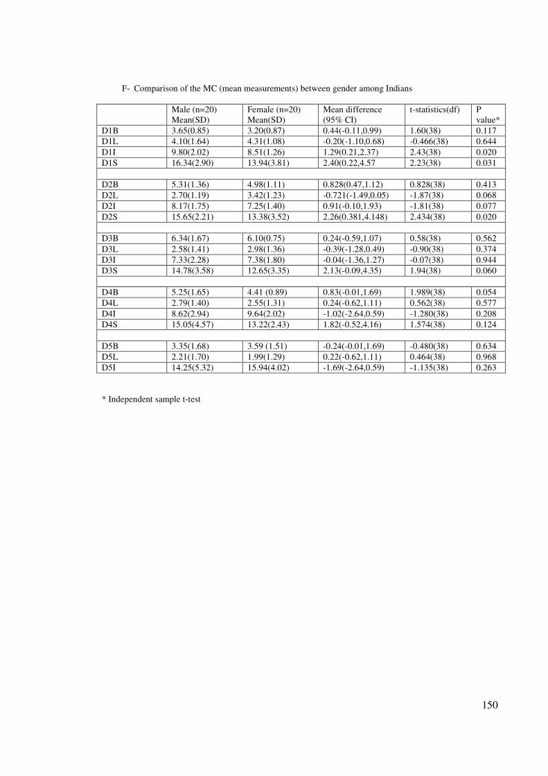
150
F- Comparison of the MC (mean measurements) between gender among Indians
Male (n=20)
Mean(SD)
Female (n=20)
Mean(SD)
Mean difference
(95% CI)
t-statistics(df) P
value*
D1B 3.65(0.85) 3.20(0.87) 0.44(-0.11,0.99) 1.60(38) 0.117
D1L 4.10(1.64) 4.31(1.08) -0.20(-1.10,0.68) -0.466(38) 0.644
D1I 9.80(2.02) 8.51(1.26) 1.29(0.21,2.37) 2.43(38) 0.020
D1S 16.34(2.90) 13.94(3.81) 2.40(0.22,4.57 2.23(38) 0.031
D2B 5.31(1.36) 4.98(1.11) 0.828(0.47,1.12) 0.828(38) 0.413
D2L 2.70(1.19) 3.42(1.23) -0.721(-1.49,0.05) -1.87(38) 0.068
D2I 8.17(1.75) 7.25(1.40) 0.91(-0.10,1.93) -1.81(38) 0.077
D2S 15.65(2.21) 13.38(3.52) 2.26(0.381,4.148) 2.434(38) 0.020
D3B 6.34(1.67) 6.10(0.75) 0.24(-0.59,1.07) 0.58(38) 0.562
D3L 2.58(1.41) 2.98(1.36) -0.39(-1.28,0.49) -0.90(38) 0.374
D3I 7.33(2.28) 7.38(1.80) -0.04(-1.36,1.27) -0.07(38) 0.944
D3S 14.78(3.58) 12.65(3.35) 2.13(-0.09,4.35) 1.94(38) 0.060
D4B 5.25(1.65) 4.41 (0.89) 0.83(-0.01,1.69) 1.989(38) 0.054
D4L 2.79(1.40) 2.55(1.31) 0.24(-0.62,1.11) 0.562(38) 0.577
D4I 8.62(2.94) 9.64(2.02) -1.02(-2.64,0.59) -1.280(38) 0.208
D4S 15.05(4.57) 13.22(2.43) 1.82(-0.52,4.16) 1.574(38) 0.124
D5B 3.35(1.68) 3.59 (1.51) -0.24(-0.01,1.69) -0.480(38) 0.634
D5L 2.21(1.70) 1.99(1.29) 0.22(-0.62,1.11) 0.464(38) 0.968
D5I 14.25(5.32) 15.94(4.02) -1.69(-2.64,0.59) -1.135(38) 0.263
* Independent sample t-test
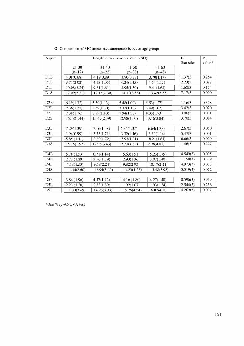
151
G- Comparison of MC (mean measurements) between age groups
Aspect Length measurements Mean (SD)
21-30
(n=12)
31-40
(n=22)
41-50
(n=38)
51-60
(n=48)
F-
Statistics
P
value*
D1B 4.08(0.68) 4.19(0.89) 3.90(0.88) 3.70(1.17)
1.37(3) 0.254
D1L 3.71(2.02) 4.13(1.05) 4.24(1.15) 4.64(1.13)
2.23(3) 0.088
D1I 10.08(2.24) 9.61(1.61) 8.95(1.50) 9.41(1.68)
1.68(3) 0.174
D1S 17.09(2.21) 17.16(2.30) 14.12(3.85) 13.82(3.63)
7.17(3) 0.000
D2B 6.19(1.32) 5.59(1.13) 5.48(1.09) 5.53(1.27)
1.16(3) 0.328
D2L 2.36(1.22) 3.59(1.30) 3.33(1.18) 3.49(1.07)
3.42(3) 0.020
D2I 7.38(1.76) 8.99(1.80) 7.94(1.38) 8.35(1.73)
3.06(3) 0.031
D2S 16.18(1.44) 15.42(2.59) 12.98(4.50) 13.46(3.84)
3.70(3) 0.014
D3B 7.29(1.39) 7.16(1.08) 6.34(1.37) 6.64(1.33)
2.67(3) 0.050
D3L 1.94(0.99) 3.73(1.71) 3.32(1.16) 3.30(1.14)
5.47(3) 0.001
D3I 5.85 (1.41) 8.60(1.72) 7.93(1.91) 8.21(1.84)
6.66(3) 0.000
D3S 15.15(1.97) 12.98(3.43) 12.33(4.82) 12.98(4.01)
1.46(3) 0.227
D4B 5.78 (1.53) 6.71(1.14) 5.63(1.51) 5.23(1.75)
4.549(3) 0.005
D4L 2.72 (1.29) 3.56(1.79) 2.93(1.36) 3.07(1.40)
1.158(3) 0.329
D4I 7.18(1.53) 9.58(2.24) 9.82(2.93) 10.17(2.21)
4.973(3) 0.003
D4S 14.66(2.60) 12.94(3.60) 13.23(4.28) 15.48(3.98)
3.319(3) 0.022
D5B 3.84 (1.96) 4.57(1.42) 4.16 (1.80) 4.27(1.40)
0.596(3) 0.919
D5L 2.23 (1.20) 2.83(1.89) 1.92(1.07) 1.93(1.34)
2.544(3) 0.256
D5I 11.80(3.69) 14.26(3.33) 15.76(4.24) 16.07(4.18)
4.269(3) 0.007
*One Way-ANOVA test
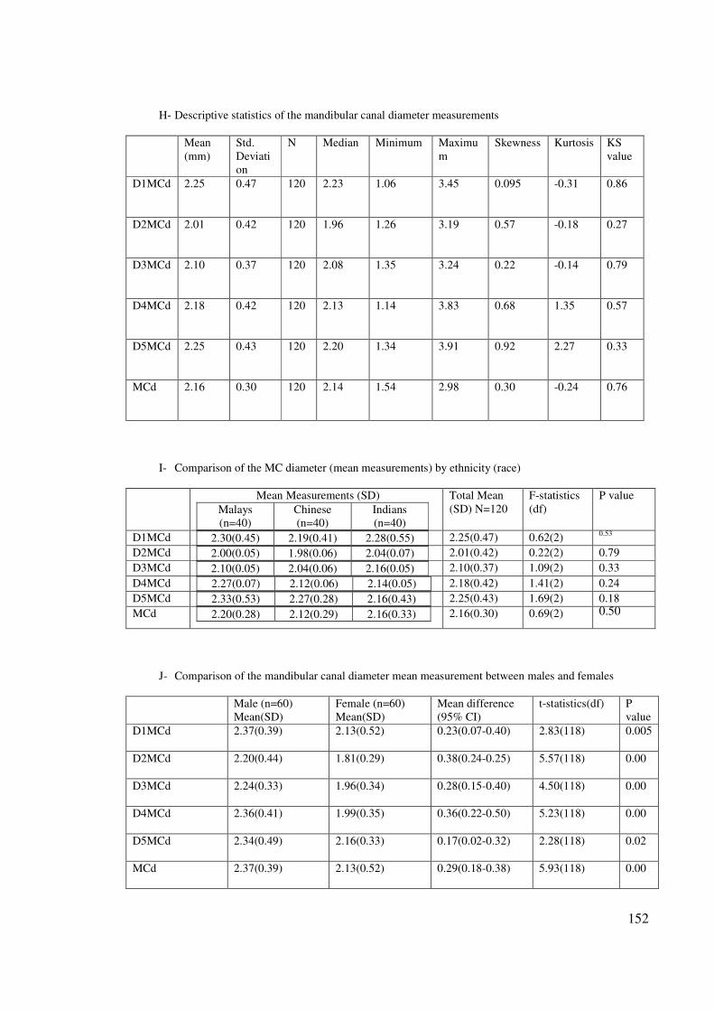
152
H- Descriptive statistics of the mandibular canal diameter measurements
Mean
(mm)
Std.
Deviati
on
N Median Minimum Maximu
m
Skewness Kurtosis KS
value
D1MCd 2.25 0.47 120 2.23 1.06 3.45 0.095 -0.31 0.86
D2MCd 2.01 0.42 120 1.96 1.26 3.19 0.57 -0.18 0.27
D3MCd 2.10 0.37 120 2.08 1.35 3.24 0.22 -0.14 0.79
D4MCd 2.18 0.42 120 2.13 1.14 3.83 0.68 1.35 0.57
D5MCd 2.25 0.43 120 2.20 1.34 3.91 0.92 2.27 0.33
MCd 2.16 0.30 120 2.14 1.54 2.98 0.30 -0.24 0.76
I- Comparison of the MC diameter (mean measurements) by ethnicity (race)
Mean Measurements (SD)
Malays
(n=40)
Chinese
(n=40)
Indians
(n=40)
Total Mean
(SD) N=120
F-statistics
(df)
P value
D1MCd 2.30(0.45) 2.19(0.41) 2.28(0.55)
2.25(0.47) 0.62(2) 0.53
D2MCd 2.00(0.05) 1.98(0.06) 2.04(0.07)
2.01(0.42) 0.22(2) 0.79
D3MCd 2.10(0.05) 2.04(0.06) 2.16(0.05)
2.10(0.37) 1.09(2) 0.33
D4MCd 2.27(0.07) 2.12(0.06) 2.14(0.05)
2.18(0.42) 1.41(2) 0.24
D5MCd 2.33(0.53) 2.27(0.28) 2.16(0.43)
2.25(0.43) 1.69(2) 0.18
MCd 2.20(0.28) 2.12(0.29) 2.16(0.33)
2.16(0.30) 0.69(2) 0.50
J- Comparison of the mandibular canal diameter mean measurement between males and females
Male (n=60)
Mean(SD)
Female (n=60)
Mean(SD)
Mean difference
(95% CI)
t-statistics(df) P
value
D1MCd 2.37(0.39) 2.13(0.52) 0.23(0.07-0.40) 2.83(118) 0.005
D2MCd 2.20(0.44) 1.81(0.29) 0.38(0.24-0.25) 5.57(118) 0.00
D3MCd 2.24(0.33) 1.96(0.34) 0.28(0.15-0.40) 4.50(118) 0.00
D4MCd 2.36(0.41) 1.99(0.35) 0.36(0.22-0.50) 5.23(118) 0.00
D5MCd 2.34(0.49) 2.16(0.33) 0.17(0.02-0.32) 2.28(118) 0.02
MCd 2.37(0.39) 2.13(0.52) 0.29(0.18-0.38) 5.93(118) 0.00
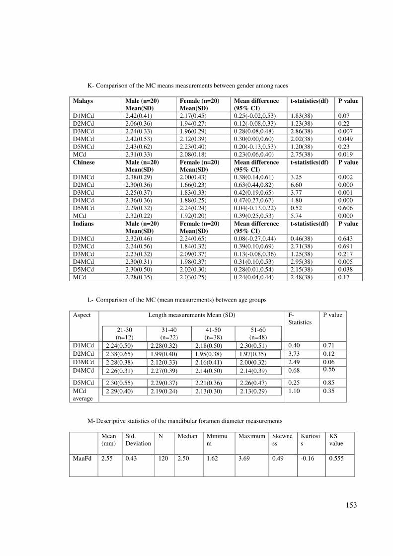
153
K- Comparison of the MC means measurements between gender among races
Malays Male (n=20)
Mean(SD)
Female (n=20)
Mean(SD)
Mean difference
(95% CI)
t-statistics(df) P value
D1MCd 2.42(0.41) 2.17(0.45) 0.25(-0.02,0.53) 1.83(38) 0.07
D2MCd 2.06(0.36) 1.94(0.27) 0.12(-0.08,0.33) 1.23(38) 0.22
D3MCd 2.24(0.33) 1.96(0.29) 0.28(0.08,0.48) 2.86(38) 0.007
D4MCd 2.42(0.53) 2.12(0.39) 0.30(0.00,0.60) 2.02(38) 0.049
D5MCd 2.43(0.62) 2.23(0.40) 0.20(-0.13,0.53) 1.20(38) 0.23
MCd 2.31(0.33) 2.08(0.18) 0.23(0.06,0.40) 2.75(38) 0.019
Chinese Male (n=20)
Mean(SD)
Female (n=20)
Mean(SD)
Mean difference
(95% CI)
t-statistics(df) P value
D1MCd 2.38(0.29) 2.00(0.43) 0.38(0.14,0.61) 3.25 0.002
D2MCd 2.30(0.36) 1.66(0.23) 0.63(0.44,0.82) 6.60 0.000
D3MCd 2.25(0.37) 1.83(0.33) 0.42(0.19,0.65) 3.77 0.001
D4MCd 2.36(0.36) 1.88(0.25) 0.47(0.27,0.67) 4.80 0.000
D5MCd 2.29(0.32) 2.24(0.24) 0.04(-0.13.0.22) 0.52 0.606
MCd 2.32(0.22) 1.92(0.20) 0.39(0.25,0.53) 5.74 0.000
Indians Male (n=20)
Mean(SD)
Female (n=20)
Mean(SD)
Mean difference
(95% CI)
t-statistics(df) P value
D1MCd 2.32(0.46) 2.24(0.65) 0.08(-0.27,0.44) 0.46(38) 0.643
D2MCd 2.24(0.56) 1.84(0.32) 0.39(0.10,0.69) 2.71(38) 0.691
D3MCd 2.23(0.32) 2.09(0.37) 0.13(-0.08,0.36) 1.25(38) 0.217
D4MCd 2.30(0.31) 1.98(0.37) 0.31(0.10,0.53) 2.95(38) 0.005
D5MCd 2.30(0.50) 2.02(0.30) 0.28(0.01,0.54) 2.15(38) 0.038
MCd 2.28(0.35) 2.03(0.25) 0.24(0.04,0.44) 2.48(38) 0.17
L- Comparison of the MC (mean measurements) between age groups
Aspect Length measurements Mean (SD)
21-30
(n=12)
31-40
(n=22)
41-50
(n=38)
51-60
(n=48)
F-
Statistics
P value
D1MCd 2.24(0.50) 2.28(0.32) 2.18(0.50) 2.30(0.51)
0.40 0.71
D2MCd 2.38(0.65) 1.99(0.40) 1.95(0.38) 1.97(0.35)
3.73 0.12
D3MCd 2.28(0.38) 2.12(0.33) 2.16(0.41) 2.00(0.32)
2.49 0.06
D4MCd 2.26(0.31) 2.27(0.39) 2.14(0.50) 2.14(0.39)
0.68 0.56
D5MCd 2.30(0.55) 2.29(0.37) 2.21(0.36) 2.26(0.47)
0.25 0.85
MCd
average 2.29(0.40) 2.19(0.24) 2.13(0.30) 2.13(0.29)
1.10 0.35
M- Descriptive statistics of the mandibular foramen diameter measurements
Mean
(mm)
Std.
Deviation
N Median Minimu
m
Maximum Skewne
ss
Kurtosi
s
KS
value
ManFd 2.55 0.43 120 2.50 1.62 3.69 0.49 -0.16 0.555
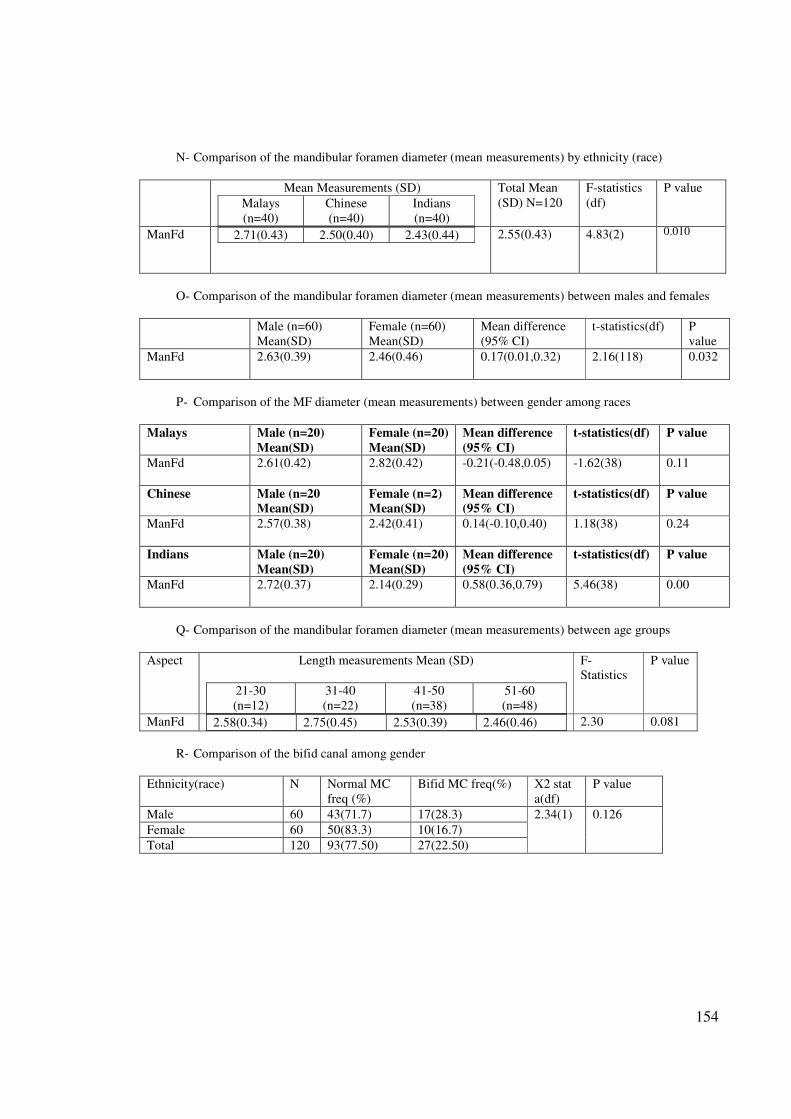
154
N- Comparison of the mandibular foramen diameter (mean measurements) by ethnicity (race)
Mean Measurements (SD)
Malays
(n=40)
Chinese
(n=40)
Indians
(n=40)
Total Mean
(SD) N=120
F-statistics
(df)
P value
ManFd 2.71(0.43) 2.50(0.40) 2.43(0.44)
2.55(0.43) 4.83(2) 0.010
O- Comparison of the mandibular foramen diameter (mean measurements) between males and females
Male (n=60)
Mean(SD)
Female (n=60)
Mean(SD)
Mean difference
(95% CI)
t-statistics(df) P
value
ManFd 2.63(0.39) 2.46(0.46) 0.17(0.01,0.32) 2.16(118) 0.032
P- Comparison of the MF diameter (mean measurements) between gender among races
Malays Male (n=20)
Mean(SD)
Female (n=20)
Mean(SD)
Mean difference
(95% CI)
t-statistics(df) P value
ManFd 2.61(0.42) 2.82(0.42) -0.21(-0.48,0.05) -1.62(38) 0.11
Chinese Male (n=20
Mean(SD)
Female (n=2)
Mean(SD)
Mean difference
(95% CI)
t-statistics(df) P value
ManFd 2.57(0.38) 2.42(0.41) 0.14(-0.10,0.40) 1.18(38) 0.24
Indians Male (n=20)
Mean(SD)
Female (n=20)
Mean(SD)
Mean difference
(95% CI)
t-statistics(df) P value
ManFd 2.72(0.37) 2.14(0.29) 0.58(0.36,0.79) 5.46(38) 0.00
Q- Comparison of the mandibular foramen diameter (mean measurements) between age groups
Aspect Length measurements Mean (SD)
21-30
(n=12)
31-40
(n=22)
41-50
(n=38)
51-60
(n=48)
F-
Statistics
P value
ManFd 2.58(0.34) 2.75(0.45) 2.53(0.39) 2.46(0.46)
2.30 0.081
R- Comparison of the bifid canal among gender
Ethnicity(race) N Normal MC
freq (%)
Bifid MC freq(%) X2 stat
a(df)
P value
Male 60 43(71.7) 17(28.3) 2.34(1) 0.126
Female 60 50(83.3) 10(16.7)
Total 120 93(77.50) 27(22.50)