Metric packing for K3 + K3

Hiroshi HIRAIResearch Institute for Mathematical Sciences,

Kyoto University, Kyoto 606-8502, Japanhirai@kurims.kyoto-u.ac.jp

October 2007April 2009 (revised)

AbstractIn this paper, we consider the metric packing problem for the commodity graph of

disjoint two triangles K3 +K3, which is dual to the multiflow feasibility problem forthe commodity graph K3 + K3. We prove a strengthening of Karzanov’s conjectureconcerning quarter-integral packings by certain bipartite metrics.

1 Introduction and main result

A metric µ on a finite set V is a function V × V → R satisfying µ(i, i) = 0, µ(i, j) =µ(j, i) ≥ 0, and the triangle inequalities µ(i, j)+µ(j, k) ≥ µ(i, k) for i, j, k ∈ V . Through-out this paper, a graph means an undirected graph. Let G = (V,E) be a graph. Fora nonnegative edge length function l : E → R+, let dG,l denote the graph metric on Vinduced by (G, l), i.e., dG,l(i, j) is the shortest path length between i and j in G withrespect to edge length l. Let dG denote the graph metric on V by G with unit edgelength.

Let H = (S,R) be another simple graph on S ⊆ V , called the commodity graph. Afinite set of metrics M on V together with its nonnegative weight λ : M → R+ is calleda fractional H-packing for (G, l) if it satisfies

l(ij) ≥∑µ∈M

λ(µ)µ(i, j) (ij ∈ E),

dG,l(s, t) =∑µ∈M

λ(µ)µ(s, t) (st ∈ R). (1.1)

If λ is integral, then it is called an integral H-packing for (G, l).A classical theorem in the network flow theory says that if H consists of a single

edge and l is integral, there is an integral H-packing by cut metrics. Here a metric dis called a cut metric if there is a set X ⊆ V such that d(i, j) = 1 if #(X ∩ {i, j}) = 1and d(i, j) = 0 otherwise. This is a polar theorem to Ford-Fulkerson’s max-flow min-cut theorem [10]. As is well-known, fractional H-packing problems are polar to themultiflow feasibility problems with commodity graph H; see [23, Chapter 70]. Themultiflow feasibility problem is: given a capacity c : E → R+ and a demand q : R → R+,find flows fst (st ∈ R) from s to t of value q(st) such that for each e ∈ E the total flowthrough e does not exceed c(e), or establish that no such a flow exists.

For a finite set of metrics M on V , an obvious necessary condition for the multiflowfeasibility ∑

ij∈E

c(ij)µ(i, j) ≥∑st∈R

q(st)µ(s, t) (µ ∈ M) (1.2)

1

(a) (b) (c)

Figure 1: (a) K4, (b) C5, and (c) the union of two stars

is also sufficient if and only if for any nonnegative length function l : E → R+ thereexists a fractional H-packing for (G, l) by M. This is a simple consequence of the linearprogramming duality.

Papernov [21] has characterized the class of commodity graphs with property thatthe cut condition, i.e., (1.2) by taking M as cut metrics, is sufficient for the multiflowfeasibility. He has shown that if H is K4, C5, or the union of two stars, then the cutcondition is sufficient, where Kn is the complete graph on n vertices, Cm is a cycle onm vertices, and a star is a graph all of whose edge have a common vertex; see Figure 1.By polarity, there exists a fractional H-packing by cut metrics in this case.

Karzanov [13] has strengthened this result to a half-integral version. Here the lengthfunction l on G is said to be cyclically even if l is integral and

∑e∈C l(e) is even for any

cycle C in G.

Theorem 1.1 ([13]). Let G be a graph with cyclically even edge length l and H acommodity graph. If H is K4, C5, or the union of two stars, then there exists an integralH-packing for (G, l) by cut metrics.

If H violates the condition of Theorem 1.1, the cut condition is not sufficient forthe multiflow feasibility, and therefore an H-packing by cut metrics does not exist ingeneral. Karzanov [14] has studied the multiflow feasibility problem for a five-vertexcommodity graph, and shown that the K2,3-metric condition is sufficient. Here, for agraph Γ on X, a metric µ on V is called a Γ -metric if there is a map φ : V → X such thatµ(i, j) = dΓ (φ(i), φ(j)) for i, j ∈ V . Kn,m denotes the complete bipartite graph withparts of n and m vertices. In particular. a cut metric is nothing but a K2-metric. TheΓ -metric condition is (1.2) by taking M as the set of Γ -metrics. By this result, thereis a fractional H-packing by cut metrics and K2,3-metrics for a five-vertex commoditygraph H. Again Karzanov [16] has strengthened it to:

Theorem 1.2 ([16]). Let G be a graph with cyclically even edge length l, and H acommodity graph. If H has at most five vertices, or is the union of K3 and a star, thenthere exists an integral H-packing for (G, l) by cut metrics and K2,3-metrics.

It is natural to ask: what is the class of commodity graphs H with the property thatthere exists a finite set G of graphs admitting an H-packing for any graph (G, l) by Γ -metrics over Γ ∈ G ? It is known that if H has a matching of three edges K2 +K2 +K2,there is no such a finite set of graphs G [16, Section 3]. Therefore, one can expectsuch fractional or integral H-packings by finite types of metrics only for the class ofcommodity graphs H without K2 + K2 + K2.

2

(d) (e)

Figure 2: (d) the union of K3 and a star, and (e) K3 + K3

K2 K2,3 K3,3 Γ,

Figure 3: K2, K2,3, K3,3, and Γ3,3

By direct case-by-case analysis, the commodity graphs H without K2 +K2 +K2 areclassified into the following:

(1) H has at most five vertices,

(2) H is the union of two stars,

(3) H is the union of K3 and a star, or

(4) H = K3 + K3, i.e., the sum of disjoint two triangles.

Theorems 1.1 and 1.2 above solve the first three cases (1-3). For the remaining last case(4), Karzanov [15] has shown that there exists a fractional H-packing by Γ3,3-metrics.Here Γ3,3 is the graph of 16 vertices and 27 edges obtained by subdividing each edgeof K3,3 and connecting each subdivided point to one new point; see Figure 3. In [16,Section 3], Karzanov conjectured that if H = K3+K3 and l is cyclically even, then thereexists an integral H-packing for (G, l) by (1/2)Γ3,3-metrics.

Our main result solves this conjecture affirmatively in a strong form, and also com-pletes the problem of the half or quarter integral H-packing by finite types of metrics.

Theorem 1.3. Let G be a graph with cyclically even edge length l, and H a commoditygraph. If H = K3 + K3, then there exists an integral H-packing by cut metrics, K2,3-metrics, K3,3-metrics, and Γ3,3-metrics.

Note that cut metrics, K2,3-metrics, and K3,3-metrics are submetrics of the half ofΓ3,3-metrics. In particular, this achieves an integral H-packing by integral metrics. It willturn out that a K3,3-metric appears at most once in H-packing (1.1) and its coefficient

3

equals 1. In a sense, a K3,3-metric summand is a half-integral residue of an integralH-packing by Γ3,3-metrics.

Our approach to Theorem 1.3 is based on Chepoi’s striking proof [5] to Karzanov’shalf-integral cut and K2,3-metric packing results above (Theorems 1.1 and 1.2). Hereduced an H-packing to the problem of decomposing the tight span of a metric space,which has been introduced independently by Isbell [12] and Dress [9]; see also Chrobakand Larmore [7]. Since Chepoi’s argument relies heavily on the classification result oftight spans of five-point metrics [9], it cannot be applied to six-vertex commodity graphH = K3 + K3. To overcome this difficulty, we introduce a notion of an H-minimalmetric, which is essentially equivalent to a metric whose extremal graph is H in thesense of Karzanov [16], and show that graph H crucially affects the geometry of tightspans of H-minimal metrics. In particular, we show that for a commodity graph Hwithout K2 + K2 + K2, the tight span of any H-minimal metric has dimension at most2. To obtain metric decomposition, we also develop a general decomposition theory of2-dimensional tight spans. Our approach is independent from the classification result,and gives a geometrical interpretation to the questions why cut, K2,3, K3,3, and Γ3,3-metrics arise, and why commodity graph H having K2 + K2 + K2 cannot be packed byfinite types of metrics.

This paper is organized as follows. In Section 2, we introduce fundamental conceptsrelated to tight spans, and describe how an H-packing problem reduces to the problemof decomposing a tight span. In Section 3, we develop a decomposition theory for 2-dimensional tight spans. Based on this, we complete the proof of our main theorem inSection 4. In Section 5, we give several remarks including a description of an O(n2)algorithm for an integral K3 + K3-packing.

Notation. We use the following notation. Let R and R+ be the set of reals andnonnegative reals, respectively. Let Z and Z+ be the set of integers and nonnegativeintegers, respectively. The set of functions from a set X to R is denoted by RX . Forp, q ∈ RX , the closed segment between p and q is denoted by [p, q]. For p, q ∈ RX ,p ≤ q means p(i) ≤ q(i) for each i ∈ X. The characteristic vector χS ∈ RX of S ⊆ X isdefined as: χS(i) = 1 for i ∈ S and χS(i) = 0 for i 6∈ S. We simply denote χ{i} by χi,which is the i-th unit vector.

For a graph G = (V,E), the edge between i, j ∈ V is denoted by ij or ji. ii meansa loop. For a graph G an subgraph G′ of G is called an isometric subgraph if dG = dG′

holds on vertices of G′. A stable set S of G is a subset of vertices such that there isno edge both of whose endpoints belong to S. For a subset S of vertices in G, theneighborhood N(S) of S is the set of vertices adjacent to S and not in S. G is calledbipartite if there exists a bipartition (A,B) of vertices into two (nonempty) stable setsA,B. G is called complete multipartite if there is a partition of vertices into nonemptystable sets such that every pair of vertices in different parts has an edge.

We often identify a metric space (S, µ) with metric µ. We shall regard a metric as anedge length on the complete graph. A metric is called a cyclically even if it is cyclicallyeven as an edge length on the complete graph. We use the standard terminology ofpolytope theory such as faces, extreme points, polyhedral complex, and so on; see [24].

2 Preliminaries

The main purpose of this section is to introduce fundamental concepts concerning tightspans, and is to describe how an H-packing problem reduces to the problem of decom-posing a tight span.

4

Let µ be a metric on a finite set S. We define two polyhedral sets Pµ and Tµ in RS

as

Pµ = {p ∈ RS | p(i) + p(j) ≥ µ(i, j) (i, j ∈ S)},

Tµ = the set of minimal elements of Pµ.

Tµ is called the tight span of µ [12, 9]. We immediately see the following characterizationof Tµ.

Lemma 2.1 (see [9]). For p ∈ Pµ, the following conditions are equivalent.

(1) p belongs to Tµ.

(2) for i ∈ S, there exists j ∈ S such that p(i) + p(j) = µ(i, j).

(3) p belongs to a bounded face of Pµ.

Therefore, Tµ is the union of bounded faces of Pµ, and thus is compact. For i ∈ S,let µi be a vector in RS defined by

µi(j) = µ(i, j) (j ∈ S). (2.1)

Namely, µi is the i-th column vector of the distance matrix µ.

Lemma 2.2 (see [9]). µi has the following properties.

(1) {µi} = Tµ ∩ {p ∈ RS | p(i) = 0} for i ∈ S.

(2) ‖µi − µj‖∞ = µ(i, j) for i, j ∈ S.

Proof. (1). Take p ∈ Tµ with p(i) = 0. Then we have p(j) ≥ µ(i, j) for j ∈ S. For k ∈ S,by Lemma 2.1 (2), there exists j ∈ S such that p(k)+p(j) = µ(k, j) ≤ µ(k, i)+µ(i, j) ≤p(k) + p(j). Therefore, p(k) = µ(k, i).

(2). µ(i, j) = |µi(i)−µj(i)| ≤ ‖µi −µj‖∞. Conversely, by the triangle inequality, wehave µ(i, j) ≥ |µ(i, k) − µ(j, k)| = |µi(k) − µj(k)| for k ∈ S.

In particular, (S, µ) is isometrically embedded into (Tµ, l∞) by (2). Next we introducea lattice (a discrete subgroup) in RS that behaves nicely with respect to the cyclicallyevenness. Let L be a lattice in RS defined as

L = {p ∈ RS | p(i) + p(j) ≡ 0 (mod 2) (i, j ∈ S)}.

Namely, L is the set of vectors all of whose components have the same parity. In otherwords, L is the union of even integer vectors and odd integer vectors.

Lemma 2.3. If µ is cyclically even, then we have

µi − µj ∈ L (i, j ∈ S).

Proof. By the cyclically evenness, we have

(µi − µj)(k) + (µi − µj)(l) = µ(i, k) − µ(j, k) + µ(i, l) − µ(j, l)≡ µ(i, k) + µ(k, j) + µ(j, l) + µ(l, j) (mod 2)≡ 0 (mod 2).

5

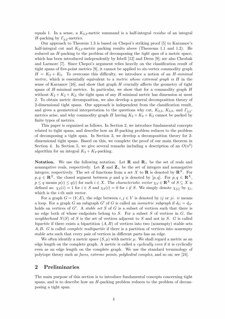
Motivated by this fact, let Aµ be an affine lattice defined by µi + L for i ∈ S. Bydefinition, it is easy to see

p(i) − q(i) ≡ p(j) − q(j) ≡ ‖p − q‖∞ (mod 2), (2.2)p(i) + p(j) − µ(i, j) ≡ 0 (mod 2) (p, q ∈ Aµ, i, j ∈ S). (2.3)

As was suggested in [5], the following discrete nonexpansive retraction plays an importantrole in H-packing problems. Here we give it in a more precise form than that given in [5,Section 2].

Proposition 2.4. Suppose that µ is a cyclically even metric on S. Then there exists amap φ : Pµ ∩ Aµ → Tµ ∩ Aµ such that

(1) ‖φ(p) − φ(q)‖∞ ≤ ‖p − q‖∞ for p, q ∈ Pµ ∩ Aµ, and

(2) φ(p) ≤ p for p ∈ Tµ ∩ Aµ, and thus φ is identical on Tµ ∩ Aµ.

Proof. Our proof is a slight modification of that in [9, (1.9)]. For i ∈ S, define a mapφi : Pµ ∩ Aµ → Pµ ∩ Aµ by

φi(p)(j) =

p(j) if j 6= i,maxk∈S\i

{µ(i, k) − p(k), 0} if j = i, p(j) ∈ 2Z,

maxk∈S\i

{µ(i, k) − p(k), 1} if j = i, p(j) 6∈ 2Z,(j ∈ S).

Note that p(i)−(µ(i, k)−p(k)) is a nonnegative even integer by p ∈ Pµ and (2.3). Namely,φi decreases the i-th component of p as much as possible belonging to Pµ∩Aµ. Clearly φi

satisfies (2). We show that φi satisfies (1). It suffices to show that |φi(p)(i)−φi(q)(i)| ≤‖p − q‖∞. Indeed, for p 6= q, we have

φi(p)(i) ≤ maxk∈S\i

{µ(i, k) − p(k), 1}

= maxk∈S\i

{µ(i, k) − q(k) + q(k) − p(k), 1}

≤ maxk∈S\i

{µ(i, k) − q(k), 1} + maxk∈S\i

{q(k) − p(k), 1}

≤ φi(q)(i) + 1 + ‖p − q‖∞.

Therefore φi(p)(i) − φi(q)(i) − ‖p − q‖∞ ≤ 1. By φi(p)(i) ≡ p(i) (mod 2) and φi(q)(i) ≡q(i) (mod 2), and (2.2), φi(p)(i) − φi(q)(i) − ‖p − q‖∞ is an even integer. Thereforeφi(p)(i) − φi(q)(i) − ‖p − q‖∞ ≤ 0. Hence |φi(p)(i) − φi(q)(i)| ≤ ‖p − q‖∞ as desired.

Let S = {i1, i2, . . . , in}. Define a map φ : Pµ ∩ Aµ → Pµ ∩ Aµ by the composition

φ = φin ◦ φin−1 ◦ · · · ◦ φi2 ◦ φi1 .

Clearly φ satisfies (1) and (2). We show that if µ 6= 0, then φ(q) ∈ Tµ ∩ Aµ for anyq ∈ Pµ ∩ Aµ. Note that if µ = 0, then Tµ = 0 and Pµ = RS

+, and the statement isobvious. Let p = φ(q). By construction of φ, for each i ∈ S, either

(i) there exists j ∈ S such that p(i) + p(j) = µ(i, j), or

(ii) p(i) = 1 and 1 + p(j) > µ(i, j) for all j ∈ S.

If there is no i ∈ S of case (ii), then we have p ∈ Tµ ∩ Aµ. If every i ∈ S is of case (ii),then µ = 0 by (2.3), and a contradiction. Suppose that there exist i, j, k ∈ S such thati is of case (ii) and p(j) + p(k) = µ(j, k). By 1 + p(j) > µ(i, j), 1 + p(k) > µ(i, k), and(2.3), we have p(j) ≥ µ(i, j) + 1 and p(k) ≥ µ(i, k) + 1. Then µ(j, k) = p(j) + p(k) ≥µ(i, j) + µ(i, k) + 2 ≥ µ(j, k) + 2. A contradiction. Thus p ∈ Tµ ∩ Aµ.

6

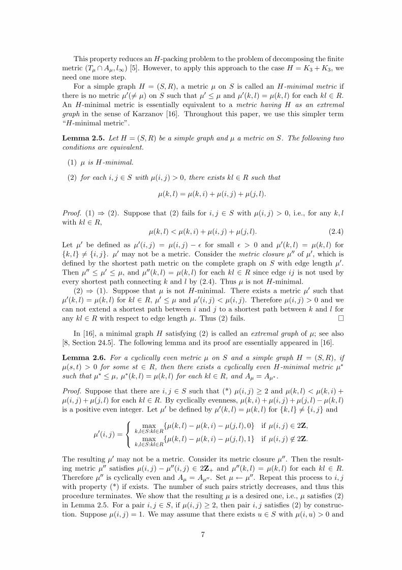
This property reduces an H-packing problem to the problem of decomposing the finitemetric (Tµ ∩Aµ, l∞) [5]. However, to apply this approach to the case H = K3 + K3, weneed one more step.

For a simple graph H = (S,R), a metric µ on S is called an H-minimal metric ifthere is no metric µ′( 6= µ) on S such that µ′ ≤ µ and µ′(k, l) = µ(k, l) for each kl ∈ R.An H-minimal metric is essentially equivalent to a metric having H as an extremalgraph in the sense of Karzanov [16]. Throughout this paper, we use this simpler term“H-minimal metric”.

Lemma 2.5. Let H = (S,R) be a simple graph and µ a metric on S. The following twoconditions are equivalent.

(1) µ is H-minimal.

(2) for each i, j ∈ S with µ(i, j) > 0, there exists kl ∈ R such that

µ(k, l) = µ(k, i) + µ(i, j) + µ(j, l).

Proof. (1) ⇒ (2). Suppose that (2) fails for i, j ∈ S with µ(i, j) > 0, i.e., for any k, lwith kl ∈ R,

µ(k, l) < µ(k, i) + µ(i, j) + µ(j, l). (2.4)

Let µ′ be defined as µ′(i, j) = µ(i, j) − ε for small ε > 0 and µ′(k, l) = µ(k, l) for{k, l} 6= {i, j}. µ′ may not be a metric. Consider the metric closure µ′′ of µ′, which isdefined by the shortest path metric on the complete graph on S with edge length µ′.Then µ′′ ≤ µ′ ≤ µ, and µ′′(k, l) = µ(k, l) for each kl ∈ R since edge ij is not used byevery shortest path connecting k and l by (2.4). Thus µ is not H-minimal.

(2) ⇒ (1). Suppose that µ is not H-minimal. There exists a metric µ′ such thatµ′(k, l) = µ(k, l) for kl ∈ R, µ′ ≤ µ and µ′(i, j) < µ(i, j). Therefore µ(i, j) > 0 and wecan not extend a shortest path between i and j to a shortest path between k and l forany kl ∈ R with respect to edge length µ. Thus (2) fails.

In [16], a minimal graph H satisfying (2) is called an extremal graph of µ; see also[8, Section 24.5]. The following lemma and its proof are essentially appeared in [16].

Lemma 2.6. For a cyclically even metric µ on S and a simple graph H = (S,R), ifµ(s, t) > 0 for some st ∈ R, then there exists a cyclically even H-minimal metric µ∗

such that µ∗ ≤ µ, µ∗(k, l) = µ(k, l) for each kl ∈ R, and Aµ = Aµ∗.

Proof. Suppose that there are i, j ∈ S such that (*) µ(i, j) ≥ 2 and µ(k, l) < µ(k, i) +µ(i, j) + µ(j, l) for each kl ∈ R. By cyclically evenness, µ(k, i) + µ(i, j) + µ(j, l)− µ(k, l)is a positive even integer. Let µ′ be defined by µ′(k, l) = µ(k, l) for {k, l} 6= {i, j} and

µ′(i, j) =

maxk,l∈S:kl∈R

{µ(k, l) − µ(k, i) − µ(j, l), 0} if µ(i, j) ∈ 2Z,

maxk,l∈S:kl∈R

{µ(k, l) − µ(k, i) − µ(j, l), 1} if µ(i, j) 6∈ 2Z.

The resulting µ′ may not be a metric. Consider its metric closure µ′′. Then the result-ing metric µ′′ satisfies µ(i, j) − µ′′(i, j) ∈ 2Z+ and µ′′(k, l) = µ(k, l) for each kl ∈ R.Therefore µ′′ is cyclically even and Aµ = Aµ′′ . Set µ ← µ′′. Repeat this process to i, jwith property (*) if exists. The number of such pairs strictly decreases, and thus thisprocedure terminates. We show that the resulting µ is a desired one, i.e., µ satisfies (2)in Lemma 2.5. For a pair i, j ∈ S, if µ(i, j) ≥ 2, then pair i, j satisfies (2) by construc-tion. Suppose µ(i, j) = 1. We may assume that there exists u ∈ S with µ(i, u) > 0 and

7

µ(j, u) > 0. Indeed, suppose that no such u exists. Then µ is necessarily a cut metric ofbipartition ({u | µ(i, u) = 0}, {u | µ(j, u) = 0}). µ(s, t) > 0 implies that µ(s, t) = 1 andedge st joins the different parts. So condition (2) is clearly fulfilled. We may assumethat µ(i, u) ≥ µ(j, u) > 0. Since µ(i, u) + µ(j, u) + µ(i, j) is even, we have µ(i, u) ≥ 2and µ(i, u) > µ(j, u). Then µ(i, j) + µ(j, u) = µ(i, u) holds. Therefore there existskl ∈ R such that µ(k, l) = µ(k, i)+µ(i, u)+µ(u, l) = µ(k, i)+µ(i, j)+µ(j, u)+µ(u, l) =µ(k, i) + µ(i, j) + µ(j, l), as required.

The following decomposition theorem is our central subject to prove the main theo-rem (Theorem 1.3). The proof is given in Section 4.

Theorem 2.7. Suppose H = (S,R) = K3 + K3. Let µ be a cyclically even H-minimalmetric on S. Then the finite metric space (Tµ ∩ Aµ, l∞) is decomposed into the sumof cut metrics, K2,3-metrics, K3,3-metrics, and Γ3,3-metrics with nonnegative integralcoefficients.

Now using this, we can derive our main theorem (Theorem 1.3) as follows. LetG = (V,E) be a connected graph, and let H = (S,R) with S ⊆ V be K3 + K3. Let lbe a cyclically even edge length function on E. Then, clearly, the graph metric dG,l isa cyclically even metric on V . Let µ be the restriction of dG,l to S. We may assumethat µ(s, t) > 0 for some st ∈ R. Otherwise the problem is trivial. By Lemma 2.6, wecan take a cyclically even H-minimal metric µ∗ with µ∗ ≤ µ, µ∗(k, l) = µ(k, l) for eachkl ∈ R, and Aµ = Aµ∗ . Consider Pµ∗ and Tµ∗ . For k ∈ V , we define a vector pk ∈ RS as

pk = µ∗k (k ∈ S) (2.5)

andpk(j) = dG,l(k, j) (j ∈ S, k ∈ V \ S). (2.6)

Then we havepk ∈ Pµ∗ ∩ Aµ∗ (k ∈ V ).

Indeed, we have pk = µ∗k ∈ Tµ∗ ∩ Aµ∗ for k ∈ S and

pk(i) + pk(j) = dG,l(k, i) + dG,l(k, j)≥ dG,l(i, j) = µ(i, j) ≥ µ∗(i, j) (k ∈ V \ S).

Therefore pk ∈ Pµ∗ for k ∈ V \S. By the cyclically evenness of dG,l and the constructionof µ∗, we have pk ∈ Aµ = Aµ∗ . Then we have

l(ij) ≥ dG,l(i, j) ≥ ‖pi − pj‖∞ (ij ∈ E),dG,l(i, j) = µ∗(i, j) = ‖pi − pj‖∞ (ij ∈ R).

Take a nonexpansive retraction φ : Pµ∗ ∩ Aµ∗ → Tµ∗ ∩ Aµ∗ in Proposition 2.4. Then weobtain

l(ij) ≥ ‖φ(pi) − φ(pj)‖∞ (ij ∈ E),dG,l(i, j) = ‖φ(pi) − φ(pj)‖∞ (ij ∈ R).

Therefore, the decomposition of (Tµ∗ ∩Aµ∗ , l∞) in Theorem 2.7 yields a required integralH-packing.

8

3 A decomposition theory for 2-dimensional tight spans

The goal of this section is to develop a decomposition theory for 2-dimensional tightspans, which is the basis for the proof of Theorem 2.7 in the next section. Let (S, µ) bea finite metric space. We further suppose that µ is cyclically even.

The first task is to represent the finite metric (Tµ ∩ Aµ, l∞) as the graph metric ofa graph obtained from the lattice L. Let Γµ be an infinite graph on vertex set Pµ ∩ Aµ

obtained by connecting p, q ∈ Pµ ∩ Aµ if ‖p − q‖∞ = 1.

Lemma 3.1. We have the following.

(1) Γµ is bipartite.

(2) dΓµ(p, q) = ‖p − q‖∞ holds for p, q ∈ Pµ ∩ Aµ.

Proof. (1). Lattice L is the disjoint union of odd vectors and even vectors. Then l∞-distances on points of the same parity are even integers. So the graph on L obtainedby connecting points with the unit l∞-distance is necessarily a bipartite graph whosebipartition is given by odd vectors and even vectors. Consequently Γµ is also bipartite.

(2). (≥) is obvious. We show the converse by constructing a path from p to qwith length ‖p − q‖∞. For p, q ∈ Pµ ∩ Aµ, let U be the set {i ∈ S | q(i) < p(i)}.Clearly, p′ := p − χU + χS\U belongs to Pµ ∩ Aµ. If p(i) 6= q(i) for all i ∈ S, then‖p − q‖∞ = 1 + ‖p′ − q‖∞. If p(i) = q(i) for some i ∈ S, then, by p − q ∈ L, we have‖p− q‖∞ ≥ 2, and therefore ‖p− q‖∞ = 1 + ‖p′− q‖∞. Repeating this process to p′ andq, we obtain the desired path.

Let Γµ be the subgraph of Γµ induced by Tµ ∩Aµ. Then Γµ is an isometric subgraphof Γµ. Indeed, for p, q ∈ Tµ ∩ Aµ, consider the image of a shortest path joining p andq in Γµ by a nonexpansive retraction in Proposition 2.4. Then this yields a shortestpath in Γµ. In particular, (Tµ ∩ Aµ, l∞) coincides with the graph metric of Γµ. Thedecomposability of the graph metric dΓµ is our central interest.

It will turn out that 2-dimensionality of Tµ is crucial for dΓµ to have a nice decom-posability property. To study the dimension of Tµ, we introduce a graph K(p) associatedwith a point p ∈ Pµ, which is a fundamental tool to investigate Tµ [9]. For p ∈ Pµ, wedefine the graph K(p) = (S,E(p)) as ij ∈ E(p) ⇔ p(i) + p(j) = µ(i, j). Namely, K(p)represents the information of facets of Pµ containing p. In particular, p ∈ Tµ if andonly if K(p) has no isolated vertices by Lemma 2.1 (2). Loop ii appears exactly whenp(i) = 0, and in this case p = µi holds by Lemma 2.2 (1). Let F (p) be the face of Tµ

containing p as its relative interior. It should be noted that

F (p) ⊆ F (q) if and only if E(p) ⊇ E(q) (p, q ∈ Pµ). (3.1)

For a face F of Tµ, we denote the corresponding graph by KF , i.e.,

KF := K(p) for a relative interior point p in a face F . (3.2)

The dimension of F (p) is characterized by a graphical property of K(p).

Lemma 3.2 ([9]). For p ∈ Tµ, we have

dimF (p) = the number of bipartite components of K(p).

Sketch of proof. dimF (p) is given by #S minus the rank of the matrix whose columnsare {χi + χj | ij ∈ E(p)}. The rank of this 0-1 matrix can be characterized in such agraphical way.

9

It turns out in the proof of the next proposition that the graph K(p) and the com-modity graph H are closely related; see Section 5.1 for further discussion. This was amotivation for the H-minimality.

Proposition 3.3. Let H = (S,R) be a simple graph and µ an H-minimal metric on S.If H has no matching of size n (n ≥ 2), then Tµ is at most (n − 1)-dimensional.

For the proof, we use the following lemma, which connects K(p) and the H-minimality.

Lemma 3.4. Let µ be an H-minimal metric. For p ∈ Tµ, if K(p) has no loops andij ∈ E(p), then there exists kl ∈ R with il, jk, kl ∈ E(p).

Proof. We note the following property of a point p ∈ Tµ [9, Theorem 3 (iv)].

p(i) + µ(i, j) ≥ p(j) (p ∈ Tµ, i, j ∈ S). (3.3)

Indeed, p(j) > p(i)+µ(i, j) implies p(j)+p(k) > p(i)+µ(i, j)+p(k) ≥ µ(i, k)+µ(i, j) ≥µ(j, k) for any k. This contradicts to Lemma 2.1 (2).

Since K(p) has no loops, p is positive, and thus µ(i, j) = p(i) + p(j) > 0. ByLemma 2.5, there exists an edge kl ∈ R such that

µ(k, l) = µ(k, i) + µ(i, j) + µ(j, l). (3.4)

By (3.3) and ij ∈ E(p), we have µ(k, l) ≥ p(k) − p(i) + p(i) + p(j) + p(l) − p(j) =p(k) + p(l) ≥ µ(k, l). This implies kl ∈ E(p). By (3.4), µ(k, j) = µ(k, i) + µ(i, j)necessarily holds. So µ(k, j) ≥ p(k)− p(i)+ p(i)+ p(j) = p(k)+ p(j) ≥ µ(k, j), and thusjk ∈ E(p). Similarly we have il ∈ E(p).

Proof of Proposition 3.3. Suppose that Tµ is n-dimensional. There exists a point p ∈ Tµ

such that K(p) has n bipartite connected components by Lemma 3.2. Then K(p) has noloops. Indeed, ii ∈ E(p) implies that p = µi (Lemma 2.2 (1)), and thus i is adjacent toall vertices. Thus K(p) is connected. A contradiction. By Lemma 3.4, each componenthas at least one edge of H, and thus H has a matching of size n.

In the case where H has no matching of size 3, Tµ is at most 2-dimensional. Toconcentrate on this case, we assume that Tµ is at most 2-dimensional in the sequel.Our next task is to investigate how the graph Γµ is drawn in Tµ. In particular, we willdetermine the connected components of

Tµ \⋃

{[p, q] | p, q ∈ Tµ ∩ Aµ, ‖p − q‖∞ = 1}.

In the subsequent arguments, the following moving process in Tµ is important.

Lemma 3.5. For p ∈ Tµ and a stable set U in K(p), we have the following.

(1) For sufficiently small ε > 0, point p + ε(−χU + χN(U)) belongs to Tµ if and only ifthere is no vertex i ∈ S \ U incident only to N(U).

(2) In addition, if p ∈ Tµ ∩ Aµ and U is maximal stable, then p − χU + χS\U belongsto Tµ ∩ Aµ.

Proof. For p ∈ Tµ, a stable set U in K(p), and small ε > 0, let pU,ε := p + ε(−χU +χN(U)). Then pU,ε ∈ Pµ. Moreover we see that K(pU,ε) is obtained by deleting all edgesconnecting N(U) and S \ U from K(p). Recall that pU,ε ∈ Tµ if and only if K(pU,ε) hasno isolated vertex (Lemma 2.1). From this fact, we have (1).

10

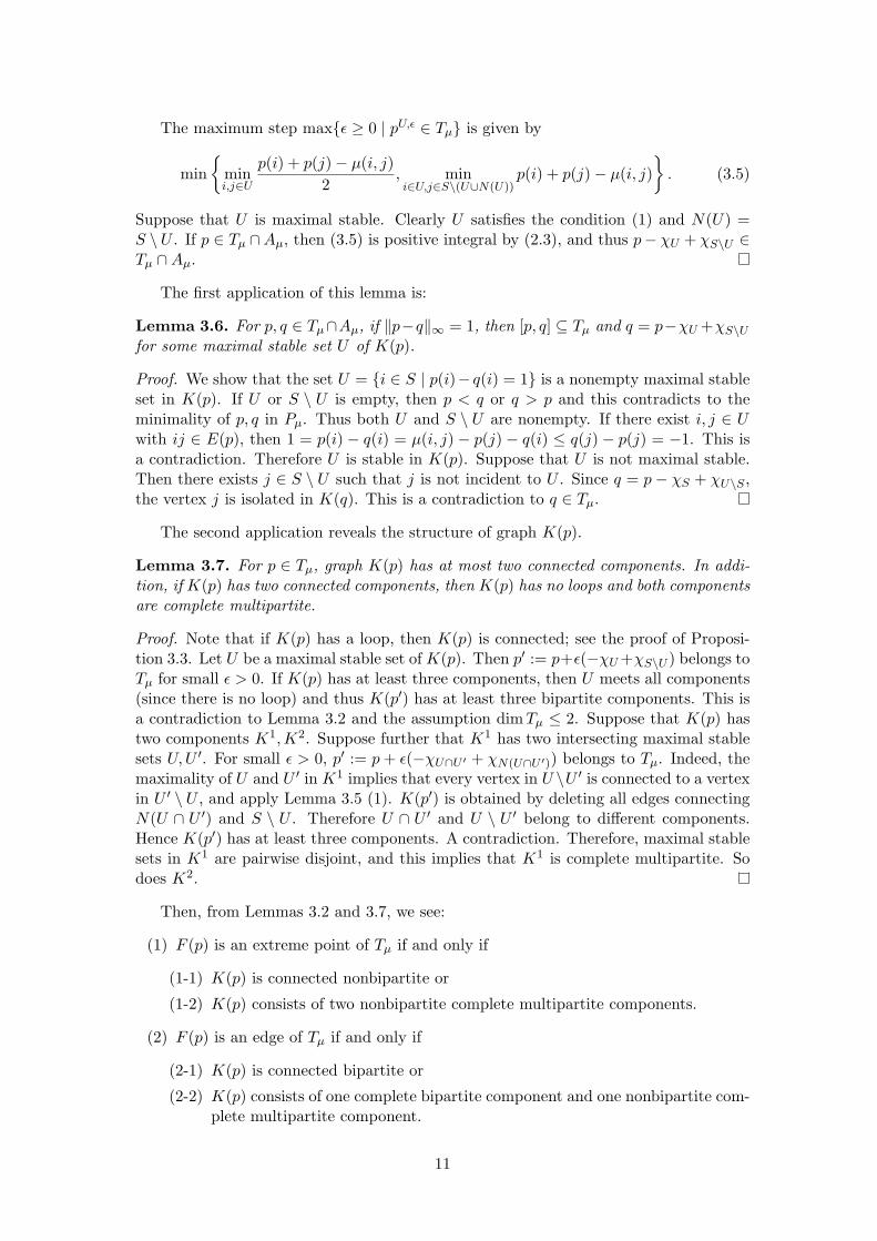
The maximum step max{ε ≥ 0 | pU,ε ∈ Tµ} is given by

min{

mini,j∈U

p(i) + p(j) − µ(i, j)2

, mini∈U,j∈S\(U∪N(U))

p(i) + p(j) − µ(i, j)}

. (3.5)

Suppose that U is maximal stable. Clearly U satisfies the condition (1) and N(U) =S \U . If p ∈ Tµ ∩Aµ, then (3.5) is positive integral by (2.3), and thus p− χU + χS\U ∈Tµ ∩ Aµ.

The first application of this lemma is:

Lemma 3.6. For p, q ∈ Tµ∩Aµ, if ‖p−q‖∞ = 1, then [p, q] ⊆ Tµ and q = p−χU +χS\Ufor some maximal stable set U of K(p).

Proof. We show that the set U = {i ∈ S | p(i)− q(i) = 1} is a nonempty maximal stableset in K(p). If U or S \ U is empty, then p < q or q > p and this contradicts to theminimality of p, q in Pµ. Thus both U and S \ U are nonempty. If there exist i, j ∈ Uwith ij ∈ E(p), then 1 = p(i) − q(i) = µ(i, j) − p(j) − q(i) ≤ q(j) − p(j) = −1. This isa contradiction. Therefore U is stable in K(p). Suppose that U is not maximal stable.Then there exists j ∈ S \ U such that j is not incident to U . Since q = p − χS + χU\S ,the vertex j is isolated in K(q). This is a contradiction to q ∈ Tµ.

The second application reveals the structure of graph K(p).

Lemma 3.7. For p ∈ Tµ, graph K(p) has at most two connected components. In addi-tion, if K(p) has two connected components, then K(p) has no loops and both componentsare complete multipartite.

Proof. Note that if K(p) has a loop, then K(p) is connected; see the proof of Proposi-tion 3.3. Let U be a maximal stable set of K(p). Then p′ := p+ε(−χU +χS\U ) belongs toTµ for small ε > 0. If K(p) has at least three components, then U meets all components(since there is no loop) and thus K(p′) has at least three bipartite components. This isa contradiction to Lemma 3.2 and the assumption dimTµ ≤ 2. Suppose that K(p) hastwo components K1,K2. Suppose further that K1 has two intersecting maximal stablesets U,U ′. For small ε > 0, p′ := p + ε(−χU∩U ′ + χN(U∩U ′)) belongs to Tµ. Indeed, themaximality of U and U ′ in K1 implies that every vertex in U \U ′ is connected to a vertexin U ′ \ U , and apply Lemma 3.5 (1). K(p′) is obtained by deleting all edges connectingN(U ∩ U ′) and S \ U . Therefore U ∩ U ′ and U \ U ′ belong to different components.Hence K(p′) has at least three components. A contradiction. Therefore, maximal stablesets in K1 are pairwise disjoint, and this implies that K1 is complete multipartite. Sodoes K2.

Then, from Lemmas 3.2 and 3.7, we see:

(1) F (p) is an extreme point of Tµ if and only if

(1-1) K(p) is connected nonbipartite or

(1-2) K(p) consists of two nonbipartite complete multipartite components.

(2) F (p) is an edge of Tµ if and only if

(2-1) K(p) is connected bipartite or

(2-2) K(p) consists of one complete bipartite component and one nonbipartite com-plete multipartite component.

11

(3) F (p) is a 2-dimensional face of Tµ if and only if K(p) consists of two completebipartite components.

In particular, there are two types of edges and extreme points. An edge e of Tµ is calledan l1-edge if Ke is connected bipartite; recall the notation (3.2). Other edge e is calledan l∞-edge. An extreme point p of Tµ is called a core if K(p) has two nonbipartitecomponents. These concepts have been introduced in [11]. Relationship among l1-edges,l∞-edges, cores, and the graph Γµ is important for us.

Lemma 3.8. Let p be an extreme point of Tµ. Then p is integral. In addition, if p isnot a core, then p ∈ Aµ.

Proof. For i ∈ S, then there exists a nonbipartite component containing i. Let C bean odd cycle of this component. We order vertices in C cyclically as (j0, j1, . . . , jm−1).Then p(j0) is given by (

∑m−1k=0 (−1)kµ(jk, jk+1))/2, where the index is taken modulo

m. By cyclically evenness, p(j0) is integral. There exists a path from i to j0 in K(p).Substituting the relation p(i′) + p(i′′) = µ(i′, i′′) along this path, we obtain p(i) which isintegral.

Next we suppose that p is not a core. Fix an odd cycle C in K(p) ordered cyclicallyas above. For any i, j ∈ S, there exist paths connecting from C to i and j, respectively.By calculation, p(i) + p(j) is given by

∑e∈P ±µ(e) for some (possibly nonsimple) path

P joining i and j. Take k ∈ S. Then we have

(µk − p)(i) + (µk − p)(j) = µ(k, i) + µ(k, j) +∑e∈P

±µ(e).

The right hand side is the sum of µ along some (possibly nonsimple) cycle in the completegraph on S, and thus even.

For an l1-edge e, if the corresponding bipartite graph Ke has a bipartition (A,B),then the direction of e is parallel to χA − χB ∈ {1,−1}S . Furthermore, we easily seethat neither endpoint of e is core (by (3.1)). Therefore each l1-edge e is a series of edgesin Γµ.

Next we study the shape of a 2-dimensional face. We simply call a 2-dimensionalface a 2-face. By calculation, we have the following; see [11] for details.

Lemma 3.9. Let F be a 2-face of Tµ. Let K1 and K2 be two bipartite components ofKF with bipartitions (A1, B1) and (A2, B2), respectively. For i ∈ A1 and j ∈ A2, theprojection map (·)|{i,j} : RS → R{i,j} is an isometry between (F, l∞) and (F |{i,j}, l∞).Moreover F |{i,j} is represented as

F |{i,j} ={

(p(i), p(j)) ∈ R2∣∣∣ a ≤ p(i) ≤ a′, c ≤ p(i) + p(j) ≤ c′,

b ≤ p(j) ≤ b′, d ≤ p(i) − p(j) ≤ d′

}for some a, a′, b, b′, c, c′, d, d′ ∈ Z.

Sketch of proof. Fix p ∈ F . Then any point q in F is uniquely represented as p+α(χA1−χB1) + β(χA2 − χB2) for some α, β ∈ R. From this, we easily see that the projection isan isometry. The coordinate p(k) for k ∈ A1 ∪ B1 is obtained by substituting relationsp(i′) + p(i′′) = µ(i′, i′′) along a path in K(p) connecting i and k in K1. From this, wesee the desired linear inequality description of F |{i,j}.

Therefore, a 2-face is isomorphic to a polygon in the l∞-plane R2 each of whoseedges is parallel to one of four vectors χ1, χ2, χ1 − χ2, and χ1 + χ2; see Figure 4 (a).

12

odd core

(R2, l∞)

(a) (b) even core

Figure 4: (a) a 2-face and (b) decomposing the 2-face by Γµ

Then l∞-edges in F are parallel to χ1 or χ2, and l1-edges in F are parallel to χ1 − χ2

or χ1 + χ2. As is well-known, the l∞-plane is isomorphic to the l1-plane by the map(x1, x2) 7→ ((x1 + x2)/2, (x1 − x2)/2); see [8, p. 31]. Then l1-edges in F are parallel tothe coordinate axes in the l1-plane. In particular, Tµ is obtained by gluing such polygonsalong the same type of edges.

Next we study the local structure around a core. In general, an edge vector ofTµ is parallel to χA − χB for some disjoint nonempty subsets A, B ⊆ S; consider theorthogonal space of vectors {χi + χj | ij ∈ E(p)} having codimension 1. By combiningLemmas 3.5 and 3.2, we see that the edge e adjacent to an extreme point p is given by[p, p + α(−χA + χN(A))] for a maximal stable set in some connected component of K(p)and a positive integer α. For a core p, if two complete multipartite components in K(p)have partitions {A1, A2, . . . , Am} and {B1, B2, . . . , Bn} (n, m ≥ 3), then we say that phas the type (A1, A2, . . . , Am; B1, B2, . . . , Bn). We denote edges adjacent to p parallel to−χAi +χ∪k 6=iAk

and −χBj +χ∪k 6=jBkby e(p,Ai) and e(p,Bj), respectively. By the above

argument and a routine verification, we have:

Lemma 3.10. Let p be a core of type (A1, A2, . . . , Am; B1, B2, . . . , Bn).

(1) An edge e is adjacent to p if and only if e is e(p,Ai) or e(p,Bj) for some i, j.

(2) Two edges e′, e′′ adjacent to p belong to the common 2-face if and only if {e′, e′′} ={e(p,Ai), e(p, Bj)} for some i, j.

We call a core p even if p ∈ Aµ, and odd if p 6∈ Aµ.

Lemma 3.11. Let p be an odd core of type (A1, A2, . . . , Am; B1, B2, . . . , Bn). For anyi, j, both p − χAi + χ∪k 6=iAk

and p − χBj + χ∪k 6=jBkbelong to Tµ ∩ Aµ.

Proof. By the argument similar to the proof of Lemma 3.8, (µl − p)(i) + (µl − p)(j) iseven for i, j ∈ ∪kAk or i, j ∈ ∪kBk. Therefore, as p 6∈ Aµ, (µl − p)(i) + (µl − p)(j) is oddfor i ∈ ∪kAk and j ∈ ∪kBk.

Summarizing these arguments, a 2-face is decomposed by Γµ as in Figure 4 (b),where the black points are vertices of Γµ, the white point is an odd core, the brokenlines represent l∞-edges, and other black lines are edges of Γµ.

Lemma 3.12. For an l∞-edge e, there exist at least three 2-faces containing e.

Proof. Let p be a relative interior point in e. Then K(p) consists of one bipartite graphand one nonbipartite graph K. The graph K is complete multipartite with partition{A1, A2, . . . , Am} (m ≥ 3). For each Ai, a point p′ := p + ε(−χAi + χ∪k 6=iAk

) for smallε > 0 belongs to Tµ by Lemma 3.5 (1). Then K(p′) has two bipartite components, andF (p′) is a 2-face.

13

(a) (b) (c)

Figure 5: (a) square, (b) K2,5-folder, and (c) K3,3-folder

Let us return back to the original problem to determine the closure of connectedcomponents of the set

Tµ \⋃

{[p, q] | p, q ∈ Tµ ∩ Aµ, ‖p − q‖∞ = 1}. (3.6)

Recall that the graph Γµ decomposes each 2-face as in Figure 4 and Tµ is obtained bygluing polygons along the same type of edges.

There are unit squares with its edges parallel to χA1∪A2−χB1∪B2 and χB1∪A2−χA1∪B2

for some four-partition {A1, A2, B1, B2} of S. We call it a square. Suppose that thereexists an l∞-edge e having two points p, q of Aµ. Then q−p is parallel to χA−χN(A) fornonmaximal stable set A of K(p). Therefore q − p is necessarily an even vector. Thenwe can take two points p, q ∈ e with ‖p− q‖∞ = 2. By Lemma 3.12, there exist m(≥ 3)2-faces containing segment [p, q]. Therefore, the closure of the component meeting thissegment is a folder obtained by gluing m right-angled isosceles triangles along their longeredge. The graph of boundary edges is the complete bipartite graph K2,m. We call it aK2,m-folder. Suppose that there exists an odd core p of type (A1, . . . , Am, B1, . . . , Bn)(m, n ≥ 3). The closure of the component containing p is the union of triangles whosevertices p, p − χAi + χ∪k 6=iAk

, and p − χBj + χ∪k 6=jBkover all pairs (i, j) of 1 ≤ i ≤ m

and 1 ≤ j ≤ n. Its boundary graph is the complete bipartite graph Kn,m. We call it aKn,m-folder. In other words, a Kn,m-folder is isomorphic to the complex of the join ofKn,m and one point. Therefore, the graph Γµ decomposes Tµ into squares, K2,l-folders,and Kn,m-folders. See Figure 5 (a), (b), and (c). Such a folder decomposition of a 2-dimensional tight span has already been obtained by [17, 18, 4] via different approach;see Section 5.3 for further discussion. Also this type of polyhedral complexes has beenstudied by Chepoi [6, Section 7]. A new point here is a relation among the lattice L,odd cores, and l1/l∞-edges.

Remark 3.13. An even core p of type (A1, . . . , Am, B1, . . . , Bn) (m,n ≥ 3) belongs ton K2,m-folders and m K2,n-folders. The union of their boundary graphs is Γn,m; seeFigure 6. Here Γn,m is the graph obtained by subdividing Kn,m and connecting eachsubdivided point to one new point. This will turn out to be a reason why Γ3,3-metricsappear in the K3 + K3-packing.

Next we discuss the decomposition of the graph metric dΓµ of Γµ. In fact, this isa special case of the decomposition of a modular graph into its orbit graphs, which isdiscussed in [3, 18, 19]. We use some of terminology in [19, Section 2] with a slightmodification. Two edges e, e′ in Γµ are called mates if there is a square containing e, e′

as its parallel edges, or there is a K2,l-folder or a Kn,m-folder containing e, e′ as its edges.

14

Figure 6: The folder structure around an even core

Two edges e, e′ in Γµ are said to be projective if there is a sequence e = e1, e2, . . . , ek = e′

such that ei and ei+1 are mates. The projectivity defines an equivalence relation on edgesof Γµ. An equivalence class is called an orbit. For an orbit O, the orbit graph ΓO

µ ofΓµ is the graph obtained by contracting all edges not in O and then identifying paralleledges appeared. By the construction, we naturally obtain a map φO from vertices of Γµ

to vertices of ΓOµ by defining φO(p) to be the contracted point. Then the graph metric

dΓµ is decomposed into the graph metrics of the orbit graphs as follows.

Proposition 3.14. Let O be the set of all orbits of Γµ. Then we have

dΓµ(p, q) =∑O∈O

dΓ Oµ

(φO(p), φO(q)) (p, q ∈ Tµ ∩ Aµ).

We will derive Theorem 2.7 from this decomposition principle, which is a simpleconsequence of the following property of shortest paths in Γµ.

Proposition 3.15. Let p, q ∈ Tµ ∩ Aµ. Let P be a shortest path connecting p and q,and Q an arbitrary path connecting p and q. For any orbit O, we have

#(P ∩ O) ≤ #(Q ∩ O).

Let P be a shortest path connecting p and q. The image of P by φO induces a pathconnecting φO(p) and φO(q) in ΓO

µ whose length is #(P ∩ O). Then φO(P ) is shortestin ΓO

µ . Suppose not. Then there exists another (not necessarily shortest) path P ′ con-necting p and q in Γµ with #(P ′∩O) < #(P ∩O). This contradicts to Proposition 3.15.Thus we have dΓµ(p, q) =

∑O∈O #(P ∩ O) =

∑O∈O dΓ O

µ(φO(p), φO(q)).

Propositions 3.14 and 3.15 hold under a more general setting [2, 18, 19, 20]; also see[8, Section 20.3]. Although one can verify that our graph Γµ belongs to the class of thegraphs treated by [2, 18, 19], we give a direct proof of Proposition 3.15. In the sequel,we often use the following distance property of Γµ:

dΓµ(u, q) − dΓµ(u′, q) ∈ {−1, 1} if u and u′ are adjacent. (3.7)

This immediately follows from the bipartiteness of Γµ (Lemma 3.1 (1)).

15

p

p1 p2

q

p

p2

q

p

F

p

p1 p2

q

p∗

(a) (b) (c)

p1

Figure 7: The quadrangle condition

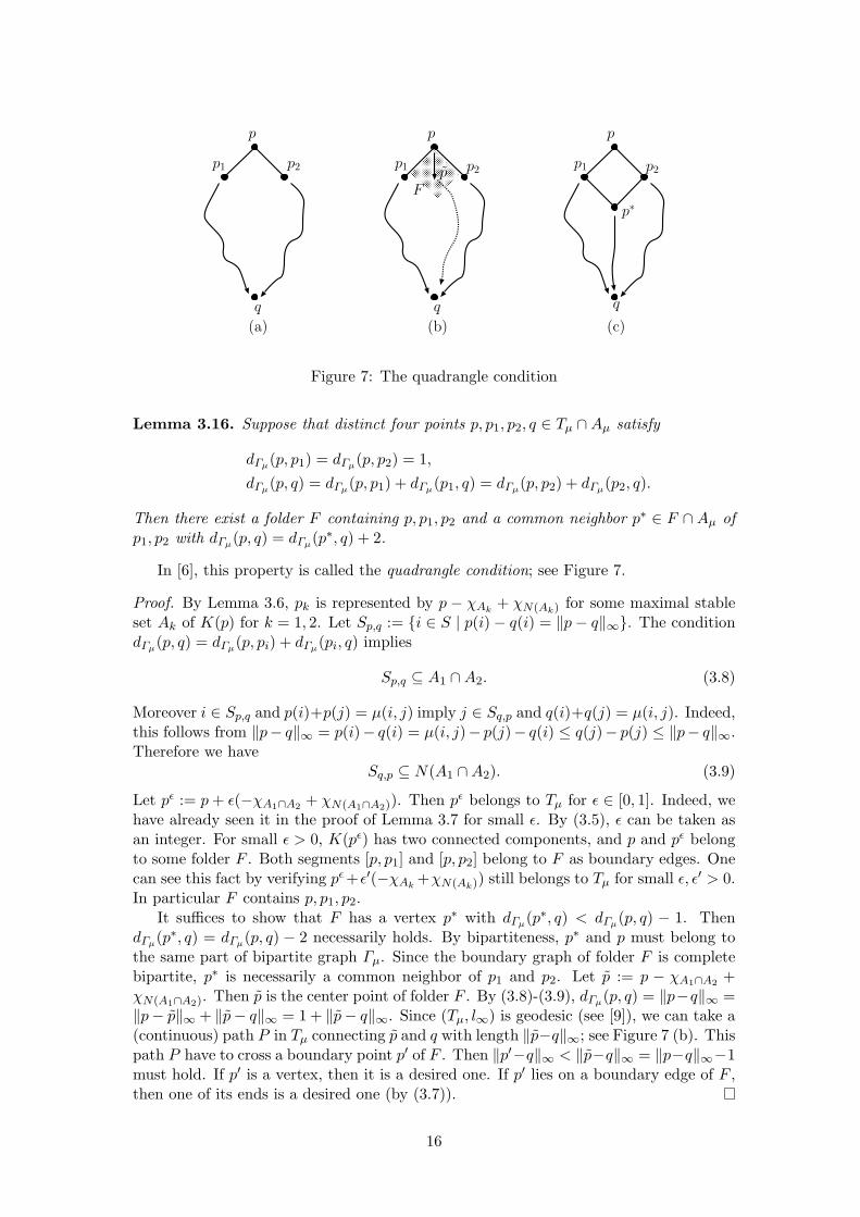
Lemma 3.16. Suppose that distinct four points p, p1, p2, q ∈ Tµ ∩ Aµ satisfy

dΓµ(p, p1) = dΓµ(p, p2) = 1,

dΓµ(p, q) = dΓµ(p, p1) + dΓµ(p1, q) = dΓµ(p, p2) + dΓµ(p2, q).

Then there exist a folder F containing p, p1, p2 and a common neighbor p∗ ∈ F ∩ Aµ ofp1, p2 with dΓµ(p, q) = dΓµ(p∗, q) + 2.

In [6], this property is called the quadrangle condition; see Figure 7.

Proof. By Lemma 3.6, pk is represented by p − χAk+ χN(Ak) for some maximal stable

set Ak of K(p) for k = 1, 2. Let Sp,q := {i ∈ S | p(i) − q(i) = ‖p − q‖∞}. The conditiondΓµ(p, q) = dΓµ(p, pi) + dΓµ(pi, q) implies

Sp,q ⊆ A1 ∩ A2. (3.8)

Moreover i ∈ Sp,q and p(i)+p(j) = µ(i, j) imply j ∈ Sq,p and q(i)+q(j) = µ(i, j). Indeed,this follows from ‖p− q‖∞ = p(i)− q(i) = µ(i, j)− p(j)− q(i) ≤ q(j)− p(j) ≤ ‖p− q‖∞.Therefore we have

Sq,p ⊆ N(A1 ∩ A2). (3.9)

Let pε := p + ε(−χA1∩A2 + χN(A1∩A2)). Then pε belongs to Tµ for ε ∈ [0, 1]. Indeed, wehave already seen it in the proof of Lemma 3.7 for small ε. By (3.5), ε can be taken asan integer. For small ε > 0, K(pε) has two connected components, and p and pε belongto some folder F . Both segments [p, p1] and [p, p2] belong to F as boundary edges. Onecan see this fact by verifying pε +ε′(−χAk

+χN(Ak)) still belongs to Tµ for small ε, ε′ > 0.In particular F contains p, p1, p2.

It suffices to show that F has a vertex p∗ with dΓµ(p∗, q) < dΓµ(p, q) − 1. ThendΓµ(p∗, q) = dΓµ(p, q) − 2 necessarily holds. By bipartiteness, p∗ and p must belong tothe same part of bipartite graph Γµ. Since the boundary graph of folder F is completebipartite, p∗ is necessarily a common neighbor of p1 and p2. Let p := p − χA1∩A2 +χN(A1∩A2). Then p is the center point of folder F . By (3.8)-(3.9), dΓµ(p, q) = ‖p−q‖∞ =‖p− p‖∞ + ‖p− q‖∞ = 1 + ‖p− q‖∞. Since (Tµ, l∞) is geodesic (see [9]), we can take a(continuous) path P in Tµ connecting p and q with length ‖p−q‖∞; see Figure 7 (b). Thispath P have to cross a boundary point p′ of F . Then ‖p′−q‖∞ < ‖p−q‖∞ = ‖p−q‖∞−1must hold. If p′ is a vertex, then it is a desired one. If p′ lies on a boundary edge of F ,then one of its ends is a desired one (by (3.7)).

16

Proof of Proposition 3.15. Suppose P = (p = u0, u1, u2, . . . , un = q) and Q = (p =v0, v1, v2, . . . , vk = q). We use the induction on k. We may assume u1 6= v1. By (3.7), wehave dΓµ(v1, q)−dΓµ(p, q) ∈ {−1, 1}. Suppose dΓµ(v1, q) = dΓµ(p, q)+1. Then P ∪{pv1}is a shortest path connecting v1 and q, and Q \ {pv1} is a path connecting v1 and q oflength k−1. By induction, we have #(Q∩O) ≥ #((Q\{pv1})∩O) ≥ #((P∪{pv1})∩O) ≥#(P ∩ O) for any orbit O. So suppose dΓµ(v1, q) = dΓµ(p, q) − 1 = dΓµ(u1, q). ApplyLemma 3.16 for quadrangle p, u1, v1, q. There exist a folder F containing p, u1, v1 and acommon neighbor p∗ of u1, v1 with dΓµ(p, q) = dΓµ(p∗, q) + 2. Let P ∗ be a shortest pathconnecting p∗ and q. Then both P \{u1p} and P ∗∪{p∗u1} are shortest paths connectingq and u1. Also P ∗ ∪ {p∗v1} is a shortest path connecting q and v1, and Q \ {v1p} isa path connecting q and v1 of length k − 1. By induction, #((P \ {u1p}) ∩ O) =#((P ∗ ∪ {p∗u1}) ∩ O) and #((Q \ {v1p}) ∩ O) ≥ #((P ∗ ∪ {p∗v1}) ∩ O). Therefore#(P ∩O) = #((P ∗∪{p∗u1, u1p})∩O) and #(Q∩O) ≥ #((P ∗∪{p∗v1, v1p})∩O). Since(p, u1, p

∗, v1) forms a cycle in folder F , by definition of orbits, p∗u1 ∈ O ⇔ v1p ∈ O andp∗v1 ∈ O ⇔ v1p ∈ O. Hence we have the desired equality #(Q ∩ O) ≥ #(P ∩ O).

4 Proof of Theorem 2.7

Let us start the proof of Theorem 2.7. Let H = (S,R) = K3 + K3. We supposeS = {1, 2, 3, 1′, 2′, 3′} and R = {12, 23, 31, 1′2′, 2′3′, 3′1′}; see Figure 8 (a). Let µ be acyclically even H-minimal metric on six-point set S. Our goal is to show that possibleorbit graphs of Γµ are K2, K2,3, K3,3, and isometric subgraphs of Γ3,3. Then the orbitgraph decomposition (Proposition 3.14) yields a desired decomposition.

Suppose that Tµ has no l∞-edges. Then Tµ is decomposed into squares. Therefore,each orbit consists of edges with parallel direction, and its orbit graph is K2. In thiscase, dΓµ is an integral sum of cut metrics, and we obtain an integral H-packing by cutmetrics; also see Section 5.1 for further discussion.

We concentrate on the case where Tµ has an l∞-edge. Recall that there exists aK2,l-folder or a Km,n-folder meeting this l∞-edge. We determine possible l,m, n. Recallthe definition (3.2) of the graph KF for a face F (and Ke for an edge e) of Tµ.

Lemma 4.1. For an l∞-edge e, either

(case 1) Ke equals H minus one edge, or

(case 2) Ke is the disjoint sum of one edge in H and K4 minus one edge containing onetriangle of H.

Proof. Ke consists of one bipartite component and one nonbipartite component. RecallLemma 3.7 that both components are complete multipartite and have no loops. ByLemma 3.4, any pair of different parts in each component is joined by an edge in H. Sincethe nonbipartite component (without loops) has at least three vertices, the bipartitecomponent has at least two vertices, and #S = 6, the nonbipartite component has threeor four vertices. Therefore Ke must be (case 1) or (case 2).

See Figure 8 (b), (c) for examples of the above two cases. By the same argument inthe proof of previous lemma, we have the following.

Lemma 4.2. If there exists a core p, then K(p) = H, and therefore p is a unique core.

Therefore, the connected components of (3.6) consist of squares, K2,3-folders, andone K3,3-folder (if an odd core exists).

17

1

2 3

1′

2′ 3′

1

2 3

1′

2′ 3′

1

2 3

1′

2′ 3′

(a) (b) (c)

Figure 8: (a) H = K3 + K3, (b) the case 1, and (c) the case 2

To investigate the orbit graph, we need to trace the orbit started from some edge.For the trace, we use the following lemma that characterizes a boundary l1-edge (corre-sponding to the case k = 1).

Lemma 4.3. An l1-edge e belongs to exactly k 2-faces if and only if Ke has exactly k+2maximal stable sets.

Proof. Ke is connected bipartite. Let (A,B) be the bipartition of Ke. Both A andB are maximal stable. Suppose that there exists another maximal stable set C. Takep ∈ e in the relative interior. Then pC,ε := p + ε(−χC + χN(C)) belongs to Tµ for smallε > 0, and K(pC,ε) has two bipartite components. Therefore the 2-face F (p′) containse. Conversely, if there exists 2-face F containing e, then there exists a maximal stableset C(6= A,B) in K(p) such that pC,ε belongs to F . For distinct maximal stable setsC ′, C ′′(6= A,B), the graphs K(pC′,ε) and K(pC′′,ε) are distinct, and hence F (pC′,ε) andF (pC′′,ε) are distinct. Thus the proof is done.

The proof of Theorem 2.7 is completed by showing:

(1) the orbit graph generated by a K3,3-folder containing odd core p is K3,3.

(2) the orbit graph generated by a K2,3-folder meeting l∞-edge e of (case 2) is K2,3.

(3) the orbit graph generated by a K2,3-folder meeting l∞-edge e of (case 1) is anisometric subgraph of Γ3,3.

Note that if an orbit meet none of Kl,m-folders, then its orbit graph is K2. In thesequel, for distinct i, j, k, l, · · · , the vector −χ{i,j,··· } + χ{k,l,··· } is denoted by χij···

kl···, suchas χ11′

232′3′(= −χ{1,1′} + χ{2,3,2′,3′}), and the graph obtained by deleting edge set E′ fromH is denoted by H − E′.

(1). Suppose that there exists an odd core p. We trace the orbit started from aboundary edge of K3,3-folder containing p. The type of p is given by (1, 2, 3; 1′, 2′, 3′).Let F11′ be the 2-face containing edges e(p, 1) and e(p, 1′), where we use the notationof Lemma 3.10 and singleton set {i} is simply denoted by i. The graph KF11′ is H −{23, 2′3′}. Since the graph Ke for an edge e of F11′ contains KF11′ as a subgraph by(3.1), it follows from Lemma 4.1 that F11′ has no l∞-edges except e(p, 1) and e(p, 1′).Therefore, the orbit started from an edge [p+χ1

23, p+χ1′2′3′ ] hits the edge e of F11′ having

direction χ12′3′231′ . The graph Ke has an edge 11′. By Lemma 4.3, this edge e is a boundary

l1-edge. Hence the orbit started from [p+χ123, p+χ1′

2′3′ ] escapes into the boundary of Tµ;see Figure 9 (a). The same holds for any i ∈ {1, 2, 3} and i′ ∈ {1′, 2′, 3′}. Therefore, theorbit started from this K3,3-folder does not meet any other K2,3-folders, and its orbitgraph is K3,3.

(2). Next we consider the orbit of a K2,3-folder meeting l∞-edge e of (case 2) inLemma 4.1. We may assume that the graph Ke is (S, {12, 23, 31, 1′2, 1′3, 2′3′}); see Fig-ure 8 (c). There exist three 2-faces F1, F2, F3 containing e. The edge sets of KF1 , KF2 ,

18

(a)

odd core p

boundary edge e

Ke

2-face F11′

KF11′

boundary

boundary

boundary

boundary

K(p)

(b)

F2

F1

F ′

1

e′

1

e1

e

e2

e1

e2

p + χ1

23

p + χ1′

2′3′

Figure 9: The orbits started from (a) K3,3-folder and (b) K2,3-folder of (case 2)

KF3 are given by {12, 13, 1′2, 1′3, 2′3′}, {12, 1′2, 23, 2′3′}, and {13, 23, 1′3, 2′3′}, respec-tively. For F1, F2, F3, the common edge e is a unique l∞-edge (by Lemma 4.1). In F2,the orbit started from this K2,3-folder hits two edges e1 and e2 of F2. Then Ke1 has anedge 22′ and Ke2 has 23′. Both e1 and e2 are in the boundary of Tµ. The same holdsfor F3. For F1, the orbit hits two edges e1 and e2 of F1 such that Ke1 has 12′ or 1′2′ (orboth), and Ke2 has 13′ or 1′3′ (or both). If Ke1 has both 12′ and 1′2′, then e1 is in theboundary. Suppose that Ke1 has only 1′2′. Then the edge e1 belongs to one more 2-faceF ′

1 with KF ′1

= (S, {13, 12, 1′2′, 2′3′}). The orbit hits an edge e′1 of F ′1. This edge e′1 is in

the boundary; see Figure 9 (b). The case where Ke1 has only 12′ does not occur sinceKF ′

1for another 2-face F ′

1 containing e1 has two components one of which has no edgeof H, which contradicts to Lemma 3.4. For e2, the argument is the same. Consequently,the orbit started from the K2,3-folder containing l∞-edge e of (case 2) does not meet anyother K2,3-folders, and its orbit graph is K2,3.

(3). Finally, we consider a K2,3-folder meeting l∞-edge of (case 1). We use somenotation. For ({i, j, k}, {i′, j′, k′}) = ({1, 2, 3}, {1′, 2′, 3′}), a 2-face F with KF = H −{jk, j′k′} is denoted by Fii′ . For {i, j, k} = {1, 2, 3} or {1′, 2′, 3′}, an l∞-edge e of (case1) with Ke = H − {jk} is denoted by ei. By (3.1), ei is the common l∞-edge of Fi1′ ,Fi2′ , Fi3′ (i = 1, 2, 3), and ei′ is the common l∞-edge of F1i′ , F2i′ , F3i′ (i′ = 1′, 2′, 3′). ByLemma 4.1, Fii′ has no l∞-edge except ei and ei′ .

Now let us trace the orbit started by a K2,3-folder F1′ meeting l∞-edge e1′ . Weshow that the orbit escapes into the boundary, or meets other K2,3-folders of (case 1)and returns to F1′ itself. Then five vertices of this K2,3-folder F1′ are given by p1′ ,p1′ + 2χ1′

2′3′ , p1′ + χi1′jk2′3′ ({i, j, k} = {1, 2, 3}) for some p1′ ∈ e1′ ∩ Aµ. The edge e1′

belongs to three 2-faces F11′ , F21′ , F31′ . The orbit started from [p1′ + 2χ1′2′3′ , p1′ + χ11′

231′2′ ]through 2-face F11′ with direction χ11′

232′3′ escapes into a boundary edge by the sameargument as in (1). However, the orbit started from [p1′ , p1′ + χ11′

232′3′ ] with directionχ12′3′

231′ may meet another nonboundary edge. Suppose that this orbit meets an l1-edge.Then this edge is in the boundary of Tµ, or belongs to another 2-face F ′. For the lattercase, the orbit further goes through F ′ and escapes into the boundary; see Figure 10 (c-2). Suppose that this orbit meets l∞-edge e1, and thus meets a K2,3-folder, which isdenoted by F1. Then five vertices of this K2,3-folder F1 are given by p1, p1 + 2χ1

23,p1 + χ1i′

23j′k′ ({i′, j′, k′} = {1′, 2′, 3′}).Similarly, this K2,3-folder F1 meets three 2-faces F11′ , F12′ , and F13′ . Again, the

orbit started from [p1 + 2χ123, p1 + χ1i′

23j′k′ ] for {i′, j′, k′} = {1′, 2′, 3′} escapes into the

19

boundary. In the 2-face F12′ , the orbit started from [p1, p1 + χ12′231′3′ ] escapes into the

boundary, or meets l∞-edge e2′ and thus a K2,3-folder F2′ . Consider the latter case.Then five vertices of this K2,3-folder F2′ are given by p2′ , p2′ + 2χ2′

1′3′ , p2′ + χi2′jk1′3′

({i, j, k} = {1, 2, 3}). Similarly, F2′ meets three 2-faces F12′ , F22′ , and F32′ . Againthe orbit started from [p2′ + 2χ2′

1′3′ , p2′ + χi2′jk1′3′ ] ({i, j, k} = {1, 2, 3}) escapes into the

boundary. In the 2-face F22′ , the orbit started from [p2′ , p2′ + χ22′131′3′ ] escapes into the

boundary, or meets l∞-edge e2 and thus meets a K2,3-folder F2. Suppose the latter case.This K2,3-folder F2 meets three 2-faces F21′ , F22′ , and F23′ . Therefore, F1′ and F2 sharethe common 2-face F21′ . Project four 2-faces F11′ , F12′ , F22′ , F21′ by the restriction map(·)|{1,1′} : RS → R{1,1′}. By Lemma 3.9, this is an injection, and we obtain a tiling bythese four 2-faces in the plane. Then edges e1′ and e2′ have the same 1-th coordinate,and edges e1 and e2 have the same 1′-th coordinate in the plane R{1,1′}. Indeed, since{p(i) + p(j) = µ(i, j), (1 ≤ i < j ≤ 3)} has full rank, the value p(1) is constant ine1′ ∪ e2′ . Therefore, in F21′ , the orbit started from [p2, p2 + χ21′

132′3′ ] returns back to thefirst K2,3-folder F1′ ; see Figure 10 (c-1).

By the same argument, the orbits started from F1′ , F2, F1, F ′2 toward other directions

escape to the boundary, or meet other Fj and return to themselves.Summarizing these arguments, this orbit O meets a subset of six K2,3-folders {Fj}j∈S .

Suppose that O meets all six K2,3-folders. Glue six K2,3-folders according to map φO

(the contraction of all edges of Γµ not belonging to O). The resulting polyhedral complexis nothing but Figure 6. Thus, the corresponding orbit graph is Γ3,3. Suppose that someof the orbits escape into the boundary instead of meeting other K2,3-folders Fj . Theresulting polyhedral complex consists of a proper subset of K2,3-folders {Fj}j∈S andsquares. A square appears as in the case of Figure 10 (c-2). Namely, the orbit startedfrom [p1′ , p1′ + χ11′

232′3′ ] hits an l1-edge in F11′ with direction χ12′3′231′ , goes through the

adjacent 2-face F ′, and escapes into the boundary, and the orbit started from [p1′ , p1′ +χ21′

131′2′ ] goes through 2-faces F21′ , F22′ , F1′2, and F ′, crosses the above orbit in F ′ andescapes into the boundary. The metric space obtained by gluing these three K2,3-foldersF1′ ,F2,F2′ and one square is a submetric of the metric space obtained by gluing fourK2,3-folders F1′ ,F2,F2′ ,F1.

Consequently, the orbit graph is an isometric subgraph of Γ3,3. We complete theproof of Theorem 2.7.

5 Remarks

In this section, we give several remarks.

5.1 H-packing by cut and K2,3-metrics

Recall Proposition 3.3 that for a commodity graph H without matching of size n, thetight span of an arbitrary H-minimal metric is at most (n− 1)-dimensional. So it wouldbe valuable to point out a further connection between commodity graph H and tightspans of H-minimal metrics.

The graphs K4, C5, and the union of two stars are exactly graphs without K2 + K3

and K2 + K2 + K2 [22]; also see [23, Theorem 72.1]. How does this condition reflect thetight span of an H-minimal metric ? The answer is:

Proposition 5.1. Let H = (S,R) be a simple graph having no K2+K3 and K2+K2+K2,and let µ be an H-minimal metric on S. Then Tµ has no l∞-edges. Consequently, everyorbit graph of Γµ is K2.

20

(c-1) (c-2)

p1′ F11′

boundarye1′

boundary

F21′

e2

F22′

boundary

e2′

F12′

e1

boundary

p1

p′

2

p2

F ′

Figure 10: The orbits started from K2,3-folder of (case 1).

Proof. Use Lemma 3.4 as in proof of Proposition 3.3 or Lemma 4.1.

From this, we obtain Karzanov’s half-integral cut packing theorem (Theorem 1.1).This is a tight-span interpretation of the shape of a commodity graph H admitting cutpacking.

The next ask is: what happens for the case that H has at most five vertices or isthe union of K3 and a star ? In this case, the tight span of any H-minimal metrichas no core; use Lemma 3.4. Therefore, Kn,m-folders for n,m ≥ 3 do not appear.However, l∞-edge e may exist. Then Ke consists of one bipartite component and onecomplete multipartite component having three parts; the proof is again similar to thatof Lemma 4.1. Therefore, the tight span is the union of squares and K2,3-folders. Bytracing the orbit of K2,3-folders as in the proof of Theorem 2.7, one can show that theorbit graph is K2,3. From this, we obtain Karzanov’s half-integral K2,3-metric packingtheorem (Theorem 1.2).

5.2 The case dim Tµ ≥ 3

Here, we explain why metric spaces (Tµ ∩Aµ, l∞) arising from 3-dimensional tight spanscannot be decomposed into finite types of metrics.

Let ΓL be the graph of L obtained by connecting a pair of points having the unitl∞-distance. If L is in the plane, then ΓL is a grid graph, and every submetric of dΓL

canbe decomposed into cut metrics. On the other hand, if the lattice L in 3-dimensionalspace, then there are infinitely many extreme submetrics in dΓL

, where a metric is calledextreme if it lies on an extreme ray of the metric cone. For example, consider thesubgraph ΓQk∩L of ΓL induced by the lattice points Qk ∩ L in the affine 3-cube

Qk = {(x1, x2, x3) ∈ R3 | 0 ≤ xi + xj ≤ 2k (1 ≤ i < j ≤ 3)}

for a positive integer k. One can show that ΓQk∩L is an isometric subgraph of ΓL, andthe corresponding graph metric dΓQk∩L

is extreme. Indeed, there are eight points inQ1 ∩ L

{(0, 0, 0), (−1, 1, 1), (1,−1, 1), (1, 1,−1), (2, 0, 0), (0, 2, 0), (0, 0, 2), (1, 1, 1)},

21

and therefore the graph ΓQ1∩L is the cube plus one diagonal edge; this graph appearsin [14, Fig 4 (b)]. It is extreme by Avis’ criterion [1]. Since Qk is obtained by pilingQ1’s, by Avis’ criterion again, dQk∩L is also extreme. Moreover one can show that foreach k there is a metric µ with dimTµ ≥ 3 such that Γµ has Qk ∩ L as an isometricsubgraph. Therefore, the graph metric dΓµ arising from 3-dimensional tight spans cannotbe decomposed into finite types of metrics. Consequently, the commodity graph Hhaving K2 + K2 + K2 cannot be packed by finite types of metrics.

5.3 The folder decomposition, modular closures, and Tµ ∩ Aµ

The folder decomposition of tight spans has already been obtained by Karzanov [18]via the method of modular closures. Here, we explain some relation among the folderdecomposition, modular closures, and the point set Tµ ∩Aµ. We need some terminologyrelated to modular metrics. The least generating graph (LG-graph) of a metric (S, µ) isthe graph on S obtained by connecting a pair i, j ∈ S if there is no k ∈ S\{i, j} such thatµ(i, j) = µ(i, k) + µ(k, j). A metric µ is called modular if for any triple k1, k2, k3 ∈ Sthere exists k∗ ∈ S, called a median, such that µ(ki, kj) = µ(ki, k

∗) + µ(k∗, kj) for1 ≤ i < j ≤ 3. A modular closure (V, µ) of a metric (S, µ) is a certain minimal modularmetric containing µ as a submetric. It is constructed by the following procedure. Initially,set V := S and µ := µ. Choose a triple s1, s2, s3 ∈ V without a median, add a new points∗ to V and define the (unique) distances from s∗ to the sk’s by

µ(s∗, sk) = (µ(sk, si) + µ(sk, sj) − µ(si, sj))/2 (5.1)

for {i, j, k} = {1, 2, 3}. Then define distances from s∗ to other points V \ {s1, s2, s3} ={s4, s5, . . . , sn} by

µ(s∗, sk) = max1≤i<k

{µ(sk, si) − µ(s∗, si)} (4 ≤ k ≤ n). (5.2)

Repeat this process for another medianless triple in the current (V, µ) until there isno medianless triple, i.e., µ is modular. Note that a modular closure µ depends on thechoice of a medianless triple {s1, s2, s3} and the ordering of V \{s1, s2, s3}. Karzanov [18]has shown that Tµ is 2-dimensional if and only if the LG-graph of a modular closure ofmetric µ is hereditary modular having no K−

3,3 as an isometric subgraph. Here a graph iscalled hereditary modular if all isometric subgraphs are modular, and K−

3,3 is K3,3 minusone edge. It is known that a graph is hereditary modular if and only if it is bipartite,and has no isometric cycles of length greater than four [3]. Furthermore, Karzanov [18]has shown that if dimTµ ≤ 2, then Tµ is obtained by filling folders appropriately intoisometric subgraphs Kn,m (n,m ≥ 2) of the LG-graph of a modular closure of µ as inFigure 5. Interestingly, a modular closure of µ is unique if dimTµ ≤ 2.

Our approach to obtain the folder decomposition might be regarded as a converseto this modular closure approach. In fact, one can show that if dimTµ ≤ 2, then Γµ

is hereditary modular without K−3,3. Moreover, a modular closure of a cyclically even

metric µ is a submetric of (Tµ ∩ Aµ, l∞). By construction, the restriction (µi)|S ofµi ∈ RV belongs to Pµ ∩ Aµ for i ∈ V , and a modular closure (V, µ) is a tight extensionof (S, µ), i.e., there is no metric µ′(6= µ) on V such that µ′ ≤ µ and µ′|S = µ|S ; see [9].Therefore (µi)|S ∈ Tµ and ‖(µi)|S − (µj)|S‖∞ = µ(i, j) for i, j ∈ V necessarily hold [9,Theorem 3], and thus (V, µ) = ({(µi)|S}i∈V , l∞) is a submetric of (Tµ ∩ Aµ, l∞).

5.4 An O(n2) algorithm for K3 + K3-packings

The proof of the main theorem is constructive, and therefore yields a strongly polynomialtime for K3 + K3-packing problems by careful modifications. Here we give an O(n2)

22

algorithm, where n is the cardinality of vertices of graph G = (V,E). The essential ideais the same as Chepoi’s O(n2) algorithm for cut and K2,3-metric packings [5].

Let G = (V,E) be a graph, H = (S,R) = K3+K3 a commodity graph on S ⊆ V , andl a cyclically even length function. An algorithm of H-packing of (G, l) by Γ3,3-metricsis the following:

(s1) Calculate dG,l(i, j) for (i, j) ∈ S × V . Let µ be the restriction of dG,l to S.

(s2) Take a cyclically even H-minimal metric µ∗ on S such that µ∗ ≤ µ, µ∗(k, l) =µ(k, l) for each kl ∈ R, and Aµ = Aµ∗ ; see Lemma 2.6.

(s3) Construct Tµ∗ .

(s4) Define vectors U := {pk}k∈V ⊆ Pµ∗ by (2.5-2.6). Calculate φ(U) for a nonexpansiveretraction φ : Pµ∗ ∩ Aµ∗ → Tµ∗ ∩ Aµ∗ in Proposition 2.4.

(s5) Decompose finite metric (φ(U), l∞) into Γ3,3-metrics.

Note that this algorithm works for any commodity graph H without K2 + K2 + K2.Let us consider the complexity. Note that the size of H is constant. (s1) can be

done in O(n log n) time by Dijkstra algorithm. (s2) can be done in the constant time;see the proof of Lemma 2.6. Also (s3) can be done in the constant time. Indeed, sincePµ∗ is a 6-dimensional polyhedron defined by 21 inequalities, the number of faces isconstant, and thus we can calculate all extreme points, all edges, all 2-faces, and theirincidence structure in the constant time. For (s4), the proof of Proposition 2.4 gives anO(n) algorithm. Indeed the calculation of 6-dimensional vector φi(pk) can be done inconstant time. Consider (s5). The size of the graph Γµ∗ is not polynomially bounded bylog(

∑i,j µ(i, j)). Therefore, a naive approach to retain Γµ∗ does not work. Instead, we

retain the incidence structure of all faces of Tµ∗ and the local 2-dimensional coordinateof each point φ(pk) in F (φ(pk)). For each φ(pk), we can identify F (φ(pk)) in constanttime; this is a membership problem in 6-dimensional space. So this can be done in O(n)time.

To identify orbit graphs of Γµ∗ , we trace orbits with their width. First, we considerthe simplest case where Tµ∗ has no l∞-edges. Note that the existence of an l∞-edge or acore can be checked in (s3). Take an arbitrary l1-edge e = [p, q]. Take an endpoint p anda point pε := p + ε(q − p) for small width ε > 0. Draw two lines from p and pε with l1-direction orthogonal to e until escaping into the boundary of Tµ∗ . Increase width ε untilthe line started from pε meets a point in φ(U) or an extreme point of Tµ∗ . This can bedone in O(n) time by operating it in each face. Note that such ε is integral. Consider thestrip sandwiched by the lines. The relative interior of this strip has no points in φ(U).Delete the relative interior of this strip from Tµ∗ . Then the resulting set consists of twoconnected components, which yields a bipartition of φ(U) and a cut-metric summand ofan H-packing with integral coefficient ε. We can determine this bipartition in O(n) time(by using the incidence information of faces). Next glue this polyhedral set along theboundary of this deleted strip by translating two components together with φ(U). Thiscan be done in O(n) time (by operating it in each face). Then we obtain a 2-dimensionalpolyhedral set smaller than Tµ∗ . Repeat the same process to this set until it becomesone point. Then we obtain an integral H-packing (by cut metrics). The number of thestrip-deletion steps will be analyzed later.

Second, we consider the case where Tµ∗ has l∞-edges and has no odd core. The ideais the same as above. Take an l∞-edge e = [p, q]. Take an endpoint p of e and a pointpε := p + ε(q − p) for small ε > 0. Draw lines having l1-direction started from p and pε

as in Figure 11 (a). Increase width ε until lines started from pε meets a point in φ(U)

23

p

(a) (b) (c)

Figure 11: (a) the strip generated by K2,3-folder, (b) deleting the strip, and (c) gluingthe components

.

or an extreme point of Tµ∗ . Note that such ε is an even integer. Then delete the stripsandwiched by these lines (Figure 11 (b)). The resulting components yields a partition ofφ(U), Again this partition can be determined in O(n) time. Then we obtain a summandof an H-packing, which is a K2,3-metric or a submetric of a Γ3,3-metric, with integralcoefficient ε/2. Gluing these components along the strip (Figure 11 (b)). Repeat thisprocess until all l∞-edge vanish. The remaining argument reduces to the first case.

Finally, we consider the case where Tµ∗ has an odd core p. Note that this oddcore is a unique core (Lemma 4.2). Consider the K3,3-folder containing p, delete thestrip generated by this K3,3-folder; recall Figure 9 (a). The resulting set consists of sixconnected components, which gives a unique K3,3-metric summand with coefficient 1.Gluing these connected components, the remaining argument reduces to the second case.

The number of the strip-deletion steps is bounded by O(n) times. Indeed, considerall lines having l1-directions started from φ(U) and extreme points of Tµ∗ . The numberof such lines is O(n). Indeed, each face has at most two lines started from each pointφ(pk); one can verify this fact by the tracing from a point in Tµ∗ as in Section 4. Eachstrip-deletion step decreases number of such lines. Consequently, we can conclude that(s5) can be done in O(n2) time, and that a desired integral H-packing can be obtainedby O(n2) time.

Acknowledgements

The author thanks the referee for careful reading and helpful suggestions. This workis supported by a Grant-in-Aid for Scientific Research from the Ministry of Education,Culture, Sports, Science and Technology of Japan.

References

[1] D. Avis, On the extreme rays of the metric cone, Canadian Journal of Mathematics32 (1980), 126–144.

[2] H.-J. Bandelt, Networks with Condorcet solutions, European Journal of OperationalResearch 20 (1985), 314–326.

24

[3] H.-J. Bandelt, Hereditary modular graphs, Combinatorica 8 (1988), 149–157.

[4] H.-J. Bandelt, V. Chepoi, and A. Karzanov, A characterization of minimizable met-rics in the multifacility location problem, European Journal of Combinatorics 21(2000), 715–725.

[5] V. Chepoi, TX -approach to some results on cuts and metrics, Advances in AppliedMathematics 19 (1997), 453–470.

[6] V. Chepoi, Graphs of some CAT(0) complexes, Advances in Applied Mathematics 24(2000), 125–179.

[7] M. Chrobak and L. L. Larmore, Generosity helps or an 11-competitive algorithm forthree servers, Journal of Algorithms 16 (1994), 234–263.

[8] M. M. Deza and M. Laurent, Geometry of Cuts and Metrics, Springer-Verlag, Berlin,(1997).

[9] A. W. M. Dress, Trees, tight extensions of metric spaces, and the cohomologicaldimension of certain groups: a note on combinatorial properties of metric spaces,Advances in Mathematics 53 (1984), 321–402.

[10] L.R. Ford and D.R. Fulkerson, Flows in networks, Princeton University Press,Princeton, 1962.

[11] H. Hirai, Tight spans of distances and the dual fractionality of undirected multiflowproblems, Journal of Combinatorial Theory, Series B, to appear.

[12] J. R. Isbell, Six theorems about injective metric spaces, Commentarii MathematiciHelvetici 39 (1964), 65–76.

[13] A. V. Karzanov, Metrics and undirected cuts, Mathematical Programming 32(1985), 183–198.

[14] A. V. Karzanov, Half-integral five-terminus flows. Discrete Applied Mathematics 18(1987), 263–278.

[15] A. V. Karzanov, Polyhedra related to undirected multicommodity flows, LinearAlgebra and its Applications 114/115 (1989), 293–328.

[16] A. V. Karzanov, Sums of cuts and bipartite metrics, European Journal of Combi-natorics 11 (1990), 473–484.

[17] A.V. Karzanov, Minimum 0-extensions of graph metrics, European Journal of Com-binatorics 19 (1998), 71–101.

[18] A. V. Karzanov, Metrics with finite sets of primitive extensions, Annals of Combi-natorics 2 (1998), 211–241.

[19] A. V. Karzanov, One more well-solved case of the multifacility location problem,Discrete Optimization 1 (2004), 51–66.

[20] M. Lomonosov and A. Sebo, On the geodesic-structure of graphs: a polyhedralapproach to metric decomposition, in: Proceedings of 3rd IPCO Conference, 1993,221–234.

25

[21] B. A. Papernov, On existence of multicommodity flows, In Studies in Discrete Op-timizations, A. A. Fridman, ed., Nauka, Moscow, 1976, 230–261 (in Russian).

[22] A. Schrijver, Short proofs on multicommodity flows and cuts, Journal of Combina-torial Theory, Series B, 53, 32–39 (1991).

[23] A. Schrijver, Combinatorial Optimization–Polyhedra and Efficiency, Springer-Verlag, Berlin, 2003.

[24] G. M. Ziegler, Lectures on Polytopes, Springer-Verlag, Berlin, 1995.

26