
Metop-A ASCAT Commissioning Quality Report
61
Metop-A ASCAT Commissioning Quality Report by EUMETSAT ASCAT Commissioning Team Craig Anderson, Hans Bonekamp, Julia Figa, Julian Wilson, Arthur de Smet, Colin Duff and EUMETSAT OSI SAF SS3 Ad Stoffelen, Anton Verhoef, Marcos Portabella, Jeroen Verspeek EUMETSAT Doc.No. : EUM/MET/REP/08/0525 Am Kavalleriesand 31, D-64295 Darmstadt, Germany Tel: +49 6151 807-7 Issue : v5 Fax: +49 6151 807 555 Date : 1 July 2009 http://www.eumetsat.int © EUMETSAT The copyright of this document is the property of EUMETSAT. It is supplied in confidence and shall not be reproduced, copied or communicated to any third party without written permission from EUMETSAT
Transcript of Metop-A ASCAT Commissioning Quality Report

Metop-A ASCAT Commissioning Quality Report
by
EUMETSAT ASCAT Commissioning Team
Craig Anderson, Hans Bonekamp, Julia Figa, Julian Wilson,
Arthur de Smet, Colin Duff
and
EUMETSAT OSI SAF SS3
Ad Stoffelen, Anton Verhoef, Marcos Portabella, Jeroen Verspeek
EUMETSAT Doc.No. : EUM/MET/REP/08/0525 Am Kavalleriesand 31, D-64295 Darmstadt, Germany
Tel: +49 6151 807-7 Issue : v5 Fax: +49 6151 807 555 Date : 1 July 2009 http://www.eumetsat.int
© EUMETSAT The copyright of this document is the property of EUMETSAT. It is supplied in confidence and shall not be reproduced, copied
or communicated to any third party without written permission from EUMETSAT

EUM/MET/REP/08/0525 v5, 1 July 2009
Metop-A ASCAT Commissioning Quality Report
Document Signature Table
Removed for Internet publication
Distribution List
Removed for Internet publication
Page 2 of 61

EUM/MET/REP/08/0525 v5, 1 July 2009
Metop-A ASCAT Commissioning Quality Report
Document Change Record
Issue / Revision
Date DCN. No
Changed Pages / Paragraphs
v4 Draft 13/06/08 Initial draft version for distribution to the SAG
v5 01/07/09 First full release.
Page 3 of 61

EUM/MET/REP/08/0525 v5, 1 July 2009
Metop-A ASCAT Commissioning Quality Report
Table of Contents
1 Introduction ..................................................................................................................................6 1.1 Purpose and Scope .............................................................................................................6 1.2 Document Outline................................................................................................................7 1.3 Applicable and Reference Documents ................................................................................7 1.4 Acronym List ........................................................................................................................8
2 Instrument Health ........................................................................................................................9 2.1 Telemetry and Configuration ...............................................................................................9 2.2 Transmit Pulse Shape .........................................................................................................9 2.3 Gain Compression Monitoring .............................................................................................9
3 Internal Calibration ....................................................................................................................11 3.1 Introduction........................................................................................................................11 3.2 Ccal Coefficients .................................................................................................................11 3.3 Receiver Gain ....................................................................................................................12 3.4 Receiver Filter Analysis .....................................................................................................13 3.5 Power Gain Product ..........................................................................................................14 3.6 Noise Power Analysis........................................................................................................15
4 External Calibration...................................................................................................................17 4.1 Introduction........................................................................................................................17 4.2 Overview ASCAT Calibration History ................................................................................17 4.3 Summary of External Calibration Procedure .....................................................................18
5 Level 1b Product Validation......................................................................................................22 5.1 Validation Using Rainforest ...............................................................................................22 5.2 Validation against ERS-2...................................................................................................23 5.3 Validation using Sea Ice ....................................................................................................24 5.4 Validation using Ocean Backscatter Models .....................................................................28 5.5 Kp Asssessment.................................................................................................................31 5.6 Level 1b Flag Assessment ................................................................................................35
6 Level 2 Product Validation........................................................................................................40 6.1 Extended Ocean Calibration..............................................................................................40
6.1.1 Introduction ...........................................................................................................40 6.1.2 Correction Factors ................................................................................................40 6.1.3 NWP Backscatter Comparison .............................................................................41 6.1.4 Wind Statistics ......................................................................................................42 6.1.5 Conclusions ..........................................................................................................43
6.2 Buoy Comparisons ............................................................................................................44 6.3 Level 2 Flag Assessments.................................................................................................46
7 Improvements to the External Calibration ..............................................................................51 7.1 Introduction........................................................................................................................51 7.2 Distortions in the Beam Pattern.........................................................................................51 7.3 Modelling the Distortions in the Gain Pattern ....................................................................53 7.4 Improved Calibration .........................................................................................................53 7.5 Reprocessed Data.............................................................................................................56
8 Overall Assessment and Recommendations..........................................................................58 8.1 Instrument Health ..............................................................................................................58 8.2 Internal Calibration ............................................................................................................58 8.3 External Calibration ...........................................................................................................58 8.4 Level 1b Product Validation...............................................................................................58
8.4.1 Rain Forest Backscatter .......................................................................................58 8.4.2 Sea Ice Backscatter..............................................................................................59 8.4.3 Ocean Backscatter ...............................................................................................59 8.4.4 Kp Assessment......................................................................................................59 8.4.5 L1b Flags ..............................................................................................................59
8.5 Level 2 Product Validation.................................................................................................60 8.5.1 Extended Ocean Calibration.................................................................................60
Page 4 of 61

EUM/MET/REP/08/0525 v5, 1 July 2009
Metop-A ASCAT Commissioning Quality Report
8.5.2 Buoy Comparisons ...............................................................................................60 8.5.3 L2 Flag Assessment .............................................................................................60
8.6 Recommendations.............................................................................................................61
Page 5 of 61

EUM/MET/REP/08/0525 v5, 1 July 2009
Metop-A ASCAT Commissioning Quality Report
1 INTRODUCTION
1.1 Purpose and Scope
This report documents the results of ASCAT calibration and validation at the start of Phase E of the ASCAT mission on Metop-A. It describes the outcome of the ASCAT calibration process and the results from the calibration and validation tests as specified in the ASCAT Test Specifications document [AD1] and as put into a logical and coherent overall form in the ASCAT Calibration and Validation Plan [AD2]. The table below provides an overview of the tests.
The ASCAT calibration and validation plan also includes the L2 wind product validation and an end-to-end assessment with the ASCAT L1b product. These aspects are summarised in this report. For details of the L2 wind product validation the reader is referred to Eumetsat’s Numerical Weather Prediction (NWP) and Ocean and Sea Ice (OSI) satellite SAF ASCAT L2 processor and product validation reports.
Table 1: Overview of ASCAT calibration and validation tests.
In order to enhance the interest of a wider audience, this report does not describe all aspects of the individual tests, but instead describes and summarises the key results as obtained for the different aspects of the commissioning as given in the ASCAT Cal Val Plan [AD2].
Important milestones before ASCAT on Metop-A reached its operational phase were the trial dissemination of a pre-validated L1b product starting on 31 January 2007, the commissioning handover on 27 April 2007 and the pre-operational status on 14 October 2007. These milestones were marked by product validation reports.
Page 6 of 61

EUM/MET/REP/08/0525 v5, 1 July 2009
Metop-A ASCAT Commissioning Quality Report
The ASCAT L1b products were declared operational on 3 April 2008, following the upgrade of the ASCAT L1b processor and configuration to version 5.6.0, which included the full absolute calibration, as derived from calibration measurements over all three ground transponders.
The draft version of this document was reviewed at the 32nd meeting of the ASCAT Science Advisory Group (SAG) and it was recommended that a small ripple seen in the calibration of the left mid antenna (beam 1) in the near range part of the swath should be corrected before reprocessing the full ASCAT data set. This refinement to the ASCAT calibration was completed at the end of 2008 and, for convenience, is also reported in this document.
It should be noted that in addition to the Cal Val tests reported on in this report, the international scatterometer community has made various studies to assess the quality of the ASCAT data not only for the ocean vector wind products but also for the soil moisture indices over land. Results have for example been discussed in the ASCAT SAG meetings Nos. 30, 31 and 32 and at international conferences and workshops.
1.2 Document Outline
Section 2 reports on the ASCAT instrument health. The results from internal and external calibration activities are presented in sections 3 and 4. Sections 5 and 6 report the results of validation activities on L1b and L2 data. Refinements to the ASCAT calibration are reported in section 7. Finally, section 8 gives an overall assessment and recommendations.
1.3 Applicable and Reference Documents
ID Title Reference
[AD1] ASCAT Calibration and Validation Test Specifications
EUM.LEO.SPE.0009 Draft D 26/10/2006
[AD2] ASCAT Calibration and Validation Plan EUM.EPS.SYS.PLN.01.011 Version 4.0 02/07/2004
[RD1] ASCAT Product Generation Function Specification (EUM.EPS.SYS.SPE.990009) Issue 6.6. 11/04/2005
[RD2] ASCAT SIOV Review Report Issue 1 MO-TN-ESA-SC-0769 26/03/2007
[RD3] Verspeek et al.: ASCAT Calibration and Validation, Technical Note
SAF/OSI/KNMI/TEC/TN/??? Draft 22/02/2007
[RD4] Hersbach H.: presentation at the 30th ASCAT SAG meeting 28-29 March 2007
[RD5] Arhuin A.: presentation at the 30th ASCAT SAG meeting 28-29 March 2007
[RD6] ASCAT Annual In-flight Performance Report Aug 2008 – Mar 2009
EUM/OPS-EPS/REP/09/0081
Page 7 of 61

EUM/MET/REP/08/0525 v5, 1 July 2009
Metop-A ASCAT Commissioning Quality Report
De Haan, S & Stoffelen, A. (2001) “Ice discrimination using ERS scatterometer”.
Hersbach, H, (2003) “CMOD5 an improved geophysical model function for ERS C band scatterometry”. ECMWF technical memorandum No. 395.
Stoffelen, A, (1999) “A simple method for calibration of a scatterometer over the ocean”. J. Atm. & Oceanic Technology, vol 16, pp 275–286.
1.4 Acronym List
The following is a list of all acronyms and abbreviations used in this report.
Acronym or Abbreviation
Definition
AGPO Antenna Gain Patterns and Orientations
ASCAT Advanced Scatterometer
Cal/Val Calibration and Validation
CGS Core Ground Segment
EPS EUMETSAT Polar System
ERS European Remote Sensing satellite (ESA)
ESA European Space Agency
EUMETCast EUMETSAT’s Data Distribution System
EUMETSAT European Organisation for the Exploitation of Meteorological Satellites
GAPE Gain at Angular Position Estimation
GCM Gain Compression Monitoring
KNMI Royal Netherlands Meteorological Institute
Kp Radiometric resolution
MDR Measurement Data Record
Metop Meteorological Operational satellite (EPS Space Segment)
NT (NTB) Normalisation Table
NTG Normalisation Table Generation
NWP Numerical Weather Prediction
OSI SAF Ocean and Sea Ice Satellite Application Facility
PPF Product Processing Facility (Level 1b processor)
PRC file Processing auxiliary parameter file
SAF Satellite Application Facility
SAG Science Advisory Group
SZO Sigma Zero Operational (Level 1b product, 50 km resolution, 25 km sampling)
SZR Sigma Zero Research (Level 1b product, 25 km resolution, 12.5 km sampling)
Page 8 of 61

EUM/MET/REP/08/0525 v5, 1 July 2009
Metop-A ASCAT Commissioning Quality Report
2 INSTRUMENT HEALTH
2.1 Telemetry and Configuration
It was planned that ASCAT instrument and platform telemetry would be written into the L1a products so that different aspects of the L1b product quality could be correlated with instrument health indicators. However, this function of the processor has not been activated for processor versions up to 5.6.0, pending the implementation of the telemetry calibration step, i.e., how to go from telemetry raw units to geophysical values. Consequently, analysis of telemetry data from the L1a product has not yet been carried out.
However, telemetry data received in the ground segment is routinely monitored in order to assess the health of the satellite and the ASCAT instrument. See e.g. [RD6] for an analysis of long term trends and instrument events.
2.2 Transmit Pulse Shape
The upgraded transponders, installed in November 2007, record the ASCAT transmitted pulse and pass the data to EUMETSAT where the pulse shape, FM rate and centre frequency can be analysed.
However, as other calibration and validation activities have taken priority, the stored data have not yet been analysed.
2.3 Gain Compression Monitoring
The monitoring of the ASCAT instrument gain compression is carried out monthly, with the purpose of checking the relationship between drive level setting and transmitted power.
In order to do that, the ASCAT instrument is operated in measurement mode with a sequence of different drive level settings and the effective transmitted power at each setting is calculated from data in the instrument source packet. The drive level and the effective transmitted power are then used to produce two summary parameters, namely:
• ptest – which measures the linear behaviour of the transmitted power with regard to drive level setting, and
• zgain – which measures the deviation of the transmitted power from the nominal value.
If ASCAT is operating nominally then the values of these parameters should not go beyond prescribed thresholds. The figure below shows the time series of ptest and zgain for the two years preceding 30 March 2009. The thresholds, marked in red, have not been exceeded.
Page 9 of 61

EUM/MET/REP/08/0525 v5, 1 July 2009
Metop-A ASCAT Commissioning Quality Report
Figure 1: Time series of the zgain and ptest parameters. Note that the horizontal axis shows the day relative to 30 March 2009.
Page 10 of 61

EUM/MET/REP/08/0525 v5, 1 July 2009
Metop-A ASCAT Commissioning Quality Report
3 INTERNAL CALIBRATION
3.1 Introduction
Several activities fall under this heading [RD1], namely: • setting the six ccal calibration constants, • setting the grx calibration constant, • analysis of the power gain product, • analysis of the receive filter shape, • analysis of noise levels.
3.2 Ccal Coefficients
Six ccal coefficients are used to set the value of the power gain product (PGP) in each beam and were calculated pre-launch as part of the instrument ground characterisation activities. These coefficients needed to be estimated again using in-orbit data. The requirements for the data to be used were:
1. The satellite nadir point should be over the ground transponders location. 2. It should be an ascending pass (night-time and hence the antennas should be more
thermally stable). 3. It should be at least 4 or 5 orbits after switch on, to ensure thermal stability.
The input L0 data selected for this procedure were: ASCA_xxx_00_M02_20061027172100Z_20061027190300Z_N_O_20061027185742Z,
along with the processing parameters and instrument parameters configuration files: ASCA_PRC_xx_M02_20060717000000Z_xxxxxxxxxxxxxxZ_20060704000100Z, ASCA_INS_xx_M02_20060717000000Z_xxxxxxxxxxxxxxZ_20060704000100Z,
Table 2 shows the original ccal and PGP values produced by the ASCAT processor for the node closest to the target lat-long for each beam. Note that the value for PGP was already very close to unity.
Rec. No. Beam Longitude Latitude ccal pgp 35784 0 26.082 39.611 9.220e-09 0.9675 36427 1 25.793 39.629 9.220e-09 0.9517 37082 2 25.799 39.633 9.220e-09 0.9509 35451 3 40.489 39.623 9.220e-09 0.9663 36088 4 40.823 39.624 9.220e-09 0.9501 36755 5 40.743 39.614 9.220e-09 0.9699
Table 2: Initial ccal values and the power gain product in the test data set.
After running again the processor with the new coefficients, the final results are shown in Table 3.
Page 11 of 61

EUM/MET/REP/08/0525 v5, 1 July 2009
Metop-A ASCAT Commissioning Quality Report
MDR Beam Longitude Latitude ccal pgp 35784 0 26.082 39.611 9.529e-09 1.0000 36427 1 25.793 39.629 9.687e-09 1.0000 37082 2 25.799 39.633 9.696e-09 1.0000 35451 3 40.489 39.623 9.541e-09 1.0000 36088 4 40.823 39.624 9.704e-09 1.0000 36755 5 40.743 39.614 9.506e-09 1.0000
Table 3: Modified ccal values and resulting power gain product.
3.3 Receiver Gain
The receiver gain grx parameter was originally planned to be set using data from one of the transponders. However, due to delays with the installation of the transponders it was decided to set the value of grx using rainforest data.
From experience with ERS-2, the parameter γ0 = σ0 /cos θ is known to be approximately -6.5 dB over rainforest and hence grx can be chosen to produce this value. The rainforest test site is taken to be the area within longitudes 70 and 63°W and latitudes 5°S and 2.5°N. Two files were selected that contained data for the left and right swaths: ASCA_SZO_1B_M02_20061030010600Z_20061030025057Z_N_C_20061030025514Z, ASCA_SZO_1B_M02_20061101002402Z_20061101020559Z_N_C_20061101021245Z.
The mean γ0 for all the data from these two files over the test site was found, 70.52 dB, and the mean γ0 in each beam is given in the following table.
Beam Mean γ0 (dB) 0 70.14 1 71.09 2 70.23 3 70.26 4 70.98 5 71.36
Table 4: Rainforest γ0 before modification of grx.
The initial grx value was 9.772×10⁹ and a new value was calculated using
grx = initial grx × 1070.52/10 / 10-6.5/10 = 4.922 × 10¹⁷
The normalisation factors used in the L1b processing to convert power into calibration backscatter needed to be derived again, using the new value of the receiver gain. However, pending at that time the validation of that part of the processor, a simple scaling of the original tables was considered as a good approximation, and the scaling factor was calculated as follows:
1070.52/10 / 10-6.5/10 = 5.038 × 10⁷
Page 12 of 61

EUM/MET/REP/08/0525 v5, 1 July 2009
Metop-A ASCAT Commissioning Quality Report
With the new value of grx and the new normalisation tables, the processor then gave an overall mean γ0 of -6.65dB which is acceptably close to the target value of -6.5 dB. This validated our scaling of the normalisation tables. The resulting γ0 in each beam is shown in the table below.
Beam Mean γ0 (dB) 0 -7.14 1 -6.17 2 -7.25 3 -7.13 4 -6.48 5 -5.95
Table 5: Rainforest γ0 resulting from new value of grx.
3.4 Receiver Filter Analysis The receive filter shape function hrx is calculated as a weighted average (in time and along discriminator frequencies) of the received noise data and is stored in L1a products. Examination of the hrx values during the first few months of ASCAT operations showed that it behaved as expected except that the values in the first few samples were negative rather than positive.
After investigation, it was found that the first sample in the noise data is always relatively large and this, in combination with one of the across-frequency averaging coefficients being negative, resulted in an overall negative value of hrx for the first few samples.
The problem was solved by changing the across-frequency averaging coefficients defined in the processing parameters file from {-0.046 -0.006 0.067 0.149 0.215 0.240 0.215 0.149 0.067 -0.006 -0.046} to {0.0 0.0 -0.046 -0.006 0.067 0.149 0.215 0.240 0.215 0.149 0.067 -0.006 -0.046 0.0 0.0}. The zeros at the end multiply the large values in the first few echo samples and thus prevent them from having any influence on the value calculated for hrx. The left-hand plot in the figure below shows a typical example of the resulting hrx function.
The hrx function has been regularly monitored since the start of ASCAT operations and has proven to be very stable. The right-hand plot in the figure below shows a two-year time series of the maximum, minimum and average hrx values and it can be seen that there is only a very small decrease over this period.
Page 13 of 61

EUM/MET/REP/08/0525 v5, 1 July 2009
Metop-A ASCAT Commissioning Quality Report
Figure 2: Left-hand plot shows a typical example of the hrx function. Right-hand plot shows a two-year time series of the maximum (red), average (black) and minimum (green)
of the hrx values.
3.5 Power Gain Product
As part of the on-board internal calibration process, ASCAT attempts to keep the transmitted power as constant as possible. Deviations from nominal power are measured by the power gain product which is calculated from data in the instrument source packets and used in the calculation of L1b backscatter.
The power gain product is routinely monitored and found to be approximately stable during normal satellite operations. A typical time series covering a 16-day period is shown in the figure below and we observe only minor changes during this time.
Figure 3: Typical time series behaviour of the power gain product. Red, green and black symbols show maximum, minimum and average values during an orbit.
Regular monitoring has also shown that • after ASCAT is reactivated after being turned off then the power gain product is larger
than usual for a few orbits before returning to normal, and
Page 14 of 61

EUM/MET/REP/08/0525 v5, 1 July 2009
Metop-A ASCAT Commissioning Quality Report
• during switch on or off of other instruments on board Metop-A the power gain product can vary.
Examples of these two types of behaviour are shown in the figure below. However, as the observed changes in magnitude are small, and are already taken into account during normal processing, the effect on L1b backscatter values is negligible.
Figure 4: Non-standard behaviour of the power gain product following ASCAT switch on (left-hand plot) and during IASI switch on (right-hand plot). Red, green and black symbols
show maximum, minimum and average power gain product during an orbit.
3.6 Noise Power Analysis
Soon after ASCAT operations had started, the measured noise values exceeded a pre-defined threshold on board which caused ASCAT to be automatically switched off. Analysis showed that ASCAT was occasionally measuring very large noise values, very likely caused by C band emission from point sources on the ground. The algorithm on board was then changed so that ASCAT needed to detect several large noise values in succession (which is unlikely from a point source) before switching off. Since then, this problem has not re-occurred.
The noise values in L0 and L1a data are routinely monitored to identify the magnitude and frequency of noise values and their geographical location. Figure 5a below shows a typical plot of the minimum and maximum noise values in L1a products over a 28-day period preceding 6 May 2008 and we can see the occasional large value caused by interference from the ground. Figure 5b below shows the ground position of all noise power values found higher than 900 during October 2007.
The impact of noise from ground sources on the σ0 values calculated by the processor has not yet been investigated in detail. However, due to the large amount of averaging performed during the calculation, the effect of a few large noise values is likely to be minimal.
Page 15 of 61

EUM/MET/REP/08/0525 v5, 1 July 2009
Metop-A ASCAT Commissioning Quality Report
(a)
(b)
Figure 5: (a) Typical time series of minimum and maximum noise values in L1a data, and (b) approximate location of noise values over 900.
Page 16 of 61

EUM/MET/REP/08/0525 v5, 1 July 2009
Metop-A ASCAT Commissioning Quality Report
4 EXTERNAL CALIBRATION
4.1 Introduction
The ASCAT ground transponders, which are located in Turkey, track the satellite as it passes overhead, receive ASCAT pulses from each of the six antennas and retransmit them with known gain. The signal received by the ASCAT varies in strength as the echoes coming from the transponders cut through the antenna gain patterns during the pass.
Given a sufficient number of passes, the full two-dimensional gain patterns for each antenna can be estimated. These are then used to derive on-board normalisation tables which allow the ASCAT measurements in power units to be converted into calibrated backscatter.
Three main processing steps required to convert the transponder data received by ASCAT into normalisation tables are:
1. Estimation of antenna gain at angular position (GAPE) – Taking into account the known gain of the transponders and their position on the ground, the transponder measurements received by ASCAT are converted into gain measurements at a corresponding position in the antenna local coordinate system.
2. Antenna gain pattern and orientation (AGPO) – A model of the antenna gain pattern is fitted to the GAPE data by finding the model parameters (depointing angles from nominal antenna position, gain scale factor, gain side lobe ratio, antenna phases and magnitudes) that minimise the difference between the model and the data.
3. Normalisation table generation (NTG) – The derived gain pattern is used to estimate the signal that would be produced by ASCAT if we assumed that the Earth’s backscatter coefficient were unity. During the L1b processing, any differences between the estimated and actual signal are assumed to be a result of the Earth’s backscatter varying from unity. Dividing the actual signal by the estimate then gives the actual backscatter. Hence the theoretically estimated signal is effectively a normalisation factor that converts ASCAT measurements into calibrated backscatter.
The GAPE, AGPO and NTG processing steps are part of the functionality of the L1b ASCAT processing software. GAPE is triggered with L0 incoming data in the EPS ground segment, while AGPO and NTG are run off-line, in order to allow further flexibility in the tuning of the involved parameters and auxiliary information. Parallel but more flexible implementations of the three processing steps were also developed in order to support trouble-shooting and tuning of the algorithms.
4.2 Overview ASCAT Calibration History
Normalisation tables were produced prior to the launch of ASCAT by assuming that the de-pointing and distortion coefficients in the gain model were zero.
Only one transponder was operational in the months immediately after launch and a small number of passes were collected during November and December 2006. Problems with the GAPE section of the processor meant that only about half of these could be processed.
Page 17 of 61

EUM/MET/REP/08/0525 v5, 1 July 2009
Metop-A ASCAT Commissioning Quality Report
However, the calibration was carried out, normalisation tables were produced and the distribution of calibrated L1b data began at the start of February 2007.
Validation of the data against rainforest indicated that the near range backscatter was too low and this was quickly found to be the result of an error in the NTG part of the processor. Revised tables were produced and used from mid-February 2007. Rainforest validation showed that the backscatter was still lower than expected. Initial users (ECMWF and KNMI) validated the L1b data against ocean backscatter models and also found some discrepancies, particularly at large incidence angles. However, they were able to compensate for this in their L2 processors and were soon able to retrieve good quality wind speeds and assimilate them in NWP models with positive results.
The GAPE and AGPO parts of the processor were improved over the following months and in September 2007 all the available transponder data were reprocessed and used for calibration. Rainforest validation with the new tables showed a decrease in backscatter levels of about 0.1 dB, taking it further away from the accepted ERS value. However, ocean validation performed by KNMI indicated that the agreement of the backscatter with CMOD5 had improved significantly at large incidence angles.
Repaired and upgraded transponders were successfully installed during November 2007 and the first calibration campaign using three transponders was performed between November 2007 and February 2008. The data collected from this period were then processed to produce new normalisation tables and this process and its results are described in sections 4, 5 and 6.
Following a review at the 32nd meeting of the ASCAT SAG, it was recommended that the calibration in beam 1 be refined in order to remove a small ripple seen in the near range backscatter. Section 7 describes this process and presents results showing that this has been achieved.
4.3 Summary of External Calibration Procedure
After quality control to remove a number of bad passes and outliers, the remaining data were used in the calibration procedure. The results from the GAPE processing step are summarised in Figure 6 which shows the peak gain values on each cut of the transponder through the beam pattern as a function of the normalised x coordinate (which is equivalent to the antenna elevation angle). The colours in the plots are used to indicate which transponder the data came from and the symbols indicate whether the pass was ascending or descending. (Note that these plots do not show the full data set and are only a section through the two-dimensional gain pattern. The data from each cut extends into and out of the plane of the paper along the azimuthal angle axis.)
Page 18 of 61

EUM/MET/REP/08/0525 v5, 1 July 2009
Metop-A ASCAT Commissioning Quality Report
Figure 6: Results from the GAPE processing step for each antenna beam. Red, green and blue indicate data from transponder 1, 2 and 3. Circles and squares indicate ascending and
descending passes.
The results from the AGPO processing step are summarised in Figure 7. This shows the difference between the maximum gain value along each cut and the fitted gain model. As above, the colours indicate transponder 1, 2 or 3 and the symbols indicate ascending or descending passes. This residual error is small, less than 0.1 dB. However there is an indication that the data from transponder 2 are biased slightly higher than those from transponders 1 and 3.
Page 19 of 61

EUM/MET/REP/08/0525 v5, 1 July 2009
Metop-A ASCAT Commissioning Quality Report
Figure 7: Summary results from the AGPO processing step showing the difference between the peak gain on each cut and the fitted gain model. Red, green and blue indicate data from transponder 1, 2 and 3. Circles and squares indicate ascending and descending
passes.
The RMS of the residuals shown in Figure 7 is given in Table 6 below. This indicates that the calibration accuracy is about 0.06 dB in most of the beams and up to 0.1 dB in beam 1.
Page 20 of 61

EUM/MET/REP/08/0525 v5, 1 July 2009
Metop-A ASCAT Commissioning Quality Report
beam RMSE (dB) 0 0.058 1 0.095 2 0.063 3 0.061 4 0.065 5 0.057
Table 6: RMS error between data and model in each of the beams.
No obvious differences between ascending and descending data are seen in Figure 7. However these plots show only results for the maximum gain along each cut. Figure 8 shows the data and fitted gain model at two different values of the azimuthal angle. On the upper line the azimuthal angle is zero (as in the plots in Figure 6), the gain takes its maximum value and the data from the ascending/descending passes lie close to the fitted model. However, on the lower line, on an azimuthal angle away from the peak, there is an obvious difference between ascending/descending data, and the fitted model lies between the two. The reason for this behaviour is suspected to be changes in the antenna pointing due to thermal effects. Its effect on the calibration is minor as the values of the two-dimensional integrals calculated in the NTG algorithm are essentially determined by the peak gain along each cut and are not affected to any significant extent by the smaller gain values away from the peak.
Figure 8: GAPE data and fitted AGPO model for two azimuthal angles in beam 0. Red, green and blue indicate data from transponder 1, 2 and 3. Circles and squares indicate
ascending and descending passes.
Page 21 of 61

EUM/MET/REP/08/0525 v5, 1 July 2009
Metop-A ASCAT Commissioning Quality Report
5 LEVEL 1B PRODUCT VALIDATION
At the beginning of February 2008, the normalisation tables generated by the calibration activities described in the previous chapter were installed in the validation ground segment, and data from this source were used for validation purposes.
5.1 Validation Using Rainforest
Rainforest areas in South America have been extensively studied using the ERS-1 and ERS-2 scatterometers. Over these areas, the parameter γ0 = σ0/cos θ is known to be approximately constant (with respect to incidence angle, geographical location and time) with a value of about -6.6 dB. This allows rainforest data to be used to check the ASCAT absolute calibration in a very simple and direct manner.
From the validation data set we took all the ASCAT SZO data (50 km resolution, 25 km spatial sampling) produced between 1 and 29 February 2008 (one complete orbital cycle), selected all data within the rainforest test area defined by longitudes 70.0 to 60.5°W, and latitudes 5°S to 2.5°N, and calculated the mean γ0. The results are shown in Table 7 below. Note that the data from ascending and descending passes are calculated separately, as experience with ERS has shown that these are slightly different.
beam ascending descending 0 -6.73 -6.61 1 -6.58 -6.47 2 -6.63 -6.57 3 -6.71 -6.59 4 -6.59 -6.46 5 -6.64 -6.60
Table 7: Mean rainforest γ0 in each beam for ascending and descending passes.
The γ0 vales in this table are within 0.1 dB of the accepted rainforest value of -6.6 dB, which gives us confidence in the calibration accuracy. The range of values over the six beams for descending and ascending passes is about 0.15 dB, indicating that the inter-beam calibration is about 0.08 dB.
Figure 9 shows the mean γ0 as a function of incidence angle. We observe variation over the incidence angle range, generally about 0.1 dB, except in beam 1 where it is larger. The origin and correction of this ripple is discussed in more detail in section 7.
Page 22 of 61

EUM/MET/REP/08/0525 v5, 1 July 2009
Metop-A ASCAT Commissioning Quality Report
Figure 9: Rainforest γ0 as a function of incidence angle.
5.2 Validation against ERS-2
ERS-2 scatterometer data over the rainforest test site contemporary to the validation data set are available and the table below compares the averages from the ERS-2 fore, mid and aft beams with the equivalent ASCAT beams 3, 4 and 5. We note that the fore and aft beams show a difference of about 0.1 dB. The value of γ0 given by the ERS-2 mid beam is unexpectedly low.
Page 23 of 61

EUM/MET/REP/08/0525 v5, 1 July 2009
Metop-A ASCAT Commissioning Quality Report
beam Ascat ERS-2 Fore -6.59 -6.49 Mid -6.59 -7.04 Aft -6.64 -6.71
Table 8: Mean rainforest γ0 in each beam.
Figure 10 below compares the ASCAT and ERS-2 average γ0 values as a function of incidence angle. For the fore and aft beams, in the incidence angle range where ERS and ASCAT overlap, there is a very close agreement between the two estimates.
Figure 10: Comparison of γ0 from ASCAT and ERS-2.
5.3 Validation using Sea Ice
Analysis using the ERS scatterometers has shown that the backscatter from regions of stable sea ice is approximately stable and can be modelled as a line in the backscatter measurement space.
We therefore examine ASCAT calibration by comparing ASCAT backscatter over regions of stable sea ice to the ‘ice line’ model developed by Haan & Stoffelen (2001) using ERS scatterometer data. Note that this model can not be taken as a reference to assess the ASCAT measurements as discussed in [AD2], because its validity in the extended incidence angle range of ASCAT is unknown, and because the ERS data from which it was derived may
Page 24 of 61

EUM/MET/REP/08/0525 v5, 1 July 2009
Metop-A ASCAT Commissioning Quality Report
contain small errors in absolute or relative calibration. Our analysis procedure consists of the following steps:
1. Find stable sea ice – we use backscatter triplets from the input data to retrieve the ice line model ‘age’ parameter and locate regions where the variability of the parameter is small and the RMS difference between the model and the data is also small.
2. Retrieve the model ‘age’ parameter – for each region of stable sea ice we obtain the best estimate of the age parameter by performing a single retrieval using all the backscatter values that occur in the region.
3. Estimate bias – for each beam and node we estimate the bias by averaging over all regions of stable sea ice the difference between the ASCAT measurement and the model backscatter produced by the ‘age’ of the region.
4. Iterate – we subtract the estimated bias from the data set and repeat steps 2 and 3 until convergence.
As our input data set we take the two-week period of ASCAT data covering 16-29 March 2008. This period should be large enough to give a reasonable-sized data set, but small enough to avoid any large changes in sea ice due to seasonal changes or ice motion.
Figure 11 shows the maps of stable sea produced from step 1 for the triplets in the left- and right-hand swaths. These are very similar, but are not expected to be exactly the same because the beams in the two swaths sample the same region at different azimuth angles and with different temporal characteristics.
Figure 11: Maps of stable sea ice produced by the beams in the left and right swaths. Stable sea ice is in white.
Page 25 of 61

EUM/MET/REP/08/0525 v5, 1 July 2009
Metop-A ASCAT Commissioning Quality Report
Figure 12 shows the ASCAT data in node 8 over the region of stable sea ice. The solid line in this figure shows the model backscatter produced by different values of the ‘age’ parameter. There is a good agreement between data and model.
Figure 12: Data and sea ice model for node 8.
However, for node 20 shown in Figure 13, the ASCAT measurements are displaced from the model and have a different slope. This could be due to errors in the model when used at the large incidence angles of nodes at the outer edge of the swath.
Figure 13: Data and sea ice mode for node 20.
Figure 14 shows the bias between the model and the ASCAT data. These results indicate that the ASCAT data and the model are generally within 0.2 dB of each other, except in beam 2 where the agreement is better than 0.1 dB. The two fore beams (beams 0 and 3) and the two mid beams (beams 1 and 4) both show similar behaviour as a function of incidence angle and, although the reason for this is not clear, it may be another sign that the model is becoming less valid at larger incidence angles.
Page 26 of 61

EUM/MET/REP/08/0525 v5, 1 July 2009
Metop-A ASCAT Commissioning Quality Report
Figure 14: Bias between ASCAT data and ice line model.
ASCAT data over stable sea ice can also be used to give an indication of the measurement noise. We take the backscatter triplets in each node, find the best fitting straight line through them and calculate the RMS difference between the data and the nearest point in the line. The results are given in Figure 15, where RMS difference is converted to Kp using
= 100.1*RMSE – 1.Kp
These estimations of Kp are higher than both the predicted instrument noise and the Kp estimations from the data and included in the L1b products (refer to the Kp assessment relevant section later on in this document). This difference needs to be understood, because it is expected that in stable areas of sea ice, the measurement noise would be very close to the instrument noise.
Page 27 of 61

EUM/MET/REP/08/0525 v5, 1 July 2009
Metop-A ASCAT Commissioning Quality Report
Figure 15: RMS difference between data and model in the left and right swaths.
5.4 Validation using Ocean Backscatter Models
Several generations of empirical ocean backscatter models have been developed from ERS-1 and ERS-2 scatterometer data. These have been primarily derived and used to retrieve near surface ocean winds from backscatter data.
Additionally, they have been very useful to assess scatterometer data calibration and noise, by comparing backscatter derived from numerical weather prediction (NWP) wind estimates against scatterometer measurements (e.g. Stoffelen 1997).
This validation technique is discussed in [AD2] and is being used by the OSI-SAF to monitor L1b and L2 products. At EUMETSAT we use a simpler procedure where we:
1. Estimate wind vector – take ASCAT backscatter measurements over the open ocean and minimise the difference between data and model by retrieving the wind vector.
2. Estimate bias – for each beam and node we estimate the bias by averaging the difference between measurement and the model backscatter produced using the estimated wind vector.
3. Iterate – we subtract the estimated bias from the data set and repeat steps 1, 2 and 3 until convergence.
This method for determining the bias between data and model works well as demonstrated by Figure 16 which compares CMOD-5 to the initial data set and to the final bias-corrected data set. It is clear that the bias-corrected data matches CMOD-5 much better than the initial data.
Page 28 of 61

EUM/MET/REP/08/0525 v5, 1 July 2009
Metop-A ASCAT Commissioning Quality Report
Figure 16: CMOD5 compared to the initial data (left-hand plot) and to the final, bias-corrected data (right-hand plot).
Figure 17 shows the bias produced by this algorithm for each beam and node. For all the side beams the bias is found to be very small, only increasing at incidence angle greater than approximately 58°. This could be caused by CMOD5 becoming less accurate at large incidence angles. The bias in the mid beams is generally larger and shows some interesting characteristics at large and small incidence angles. The large mid beam bias at incidence angles greater than approximately 47° occurs in the same nodes in which the bias also increases in the side beams. As the algorithm uses all three beams simultaneously to retrieve wind speed, it may be the case that if CMOD5 is becoming less accurate for the side beams in these nodes, this is then having some side effects for the mid beams resulting in an artificially large bias. The bias in beam 1 at lower incidence angles has two distinct peaks and this strongly resembles the results from the rainforest analysis in Figure 9.
Page 29 of 61

EUM/MET/REP/08/0525 v5, 1 July 2009
Metop-A ASCAT Commissioning Quality Report
Figure 17: Bias between ASCAT data and CMOD5.
This approach can also give an indication of the noise in the backscatter by looking at the root mean square difference between the bias-corrected backscatter triplets in each node and the nearest point in the model backscatter. Figure 18 shows the results (with the RMS difference converted to Kp) and we find that the noise is generally smaller than that seen in the sea ice analysis, but still significantly higher than predicted instrument noise and also than the Kp value estimated from the data and included in the L1b products over ocean areas (refer to the relevant Kp assessment section later on in this document).
Page 30 of 61

EUM/MET/REP/08/0525 v5, 1 July 2009
Metop-A ASCAT Commissioning Quality Report
Figure 18: RMS difference between ASCAT data and CMOD5 in the left and right swaths.
5.5 Kp Asssessment
The σ0 values in the L1b SZO and SZR products are weighted spatial averages of the full resolution σ0 measurements. The Kp values also given in these products is the estimated standard deviation in the given value of σ0 normalised by dividing it by σ0. Note that correlations between neighbouring full resolution σ0 values are taken into account when calculating Kp.
The values of Kp are generally found to be under 3%, with land targets being a bit higher than ocean targets. Both over land and ocean, high values for the mid left beam around node 15 are observed, for which no explanation exists at the moment (see Figure 19).
For non-homogeneous targets, which contain a mixture of land and ocean, the Kp values are larger, typically up to 5%, and their incidence angle dependency also changes (see Figure 20).
Much higher individual values of Kp can however be found (see Figure 21). These high values of Kp do appear to have a geographical signature, but are in any case not often higher than 20% (see Figure 22).
In summary, the Kp values seem to be on average within the specified instrument noise (3%), but because of the nature of their estimation as a standard error associated with a spatial averaging, they contain a geophysical signature, which can bring them up to higher values. Values over 20% are rare and normally associated with very low values of σ0.
Page 31 of 61

EUM/MET/REP/08/0525 v5, 1 July 2009
Metop-A ASCAT Commissioning Quality Report
Figure 19: Average Kp values over ocean (top) and land (bottom) targets per node. Left and right correspond to left and right swath. Fore beam is in red, mid beam is in green and aft
beam is in blue. Values calculated over a week of data between 11 and 19 May 2008.
Page 32 of 61

EUM/MET/REP/08/0525 v5, 1 July 2009
Metop-A ASCAT Commissioning Quality Report
Figure 20: Average Kp values over nodes corresponding to approximately 50% land and ocean. Left and right correspond to left and right swath. Fore beam is in red, mid beam is in green and aft beam is in blue. Values calculated over a week of data between 11 and 19
May 2008.
Figure 21: Time series of Kp values for fore left beam. Black squares, green diamonds and red diamonds are average, minimum and maximum values per orbit, respectively. Plots for
the other beams look very similar.
Page 33 of 61

EUM/MET/REP/08/0525 v5, 1 July 2009
Metop-A ASCAT Commissioning Quality Report
Figure 22: Maps of Kp values for the fore beams in the ranges of 6-20% (top) and 20-100% (bottom). In the top map, the continents contour has not been plotted in order to better
appreciate how many of the Kp values in that range occur in coastal areas. Values extracted from a week of data between 11 and 19 May 2008. Plots for the other beams look
very similar.
Page 34 of 61
EUM/MET/REP/08/0525 v5, 1 July 2009
Metop-A ASCAT Commissioning Quality Report
5.6 Level 1b Flag Assessment
L1b data contain a number of flags that indicate the quality of the σ0 and Kp values. The summary flags that take an integer value are:
• F_USABLE – summary flag for σ0 (0, 1, 2 indicate good, usable, bad), • F_KP – Kp quality flag (0 and 1 indicate good and bad).
The remaining flags take a value from 0 to 1 (where 0 indicates the highest quality) and are: • F_F – synthetic data have been used to fill data gaps, • F_V – if amount of synthetic data used is above a configurable threshold, • F_OA – quality of satellite orbit and attitude, • F_SA – data may be corrupted by solar array reflections (affecting the left fore beam on
descending passes only), • F_TEL – instrument and satellite housekeeping telemetry data are present and within
limits, • F_EXT_FIL – extrapolated filter shape has been used to correct data, • F_LAND – amount of land contamination in σ0.
Additionally, we can configure the processor to set F_USABLE directly to 2 in order to reflect the instrument and/or product status. This was the case until processor version 5.3.1. From 5.6.0, the products were considered operational and the calibration complete, hence F_USABLE is not determined by the configuration but based solely on a summary of the other flags.
F_TEL is currently never set. It is planned to implement this flag at a later stage.
F_F and F_V have not been validated yet, due to minor processing problems associated with the handling of small gaps in the data stream. However, this type of event is rare and activities are ongoing to ensure the robustness of the processor and the validity of these flags.
We have done a sanity check on F_LAND to verify that it is set as expected (Figure 23). As with other L1b product flags, the F_LAND flag is a fraction value over the node. It remains still to be assessed, what fraction of land contamination affects the L2 wind retrieval and what fraction of ocean contamination affects the L2 soil moisture retrieval in coastal areas.
F_KP is set when the value of Kp is set to 1.0 or missing. Kp is set to 1.0 when its calculation according to [RD1] results in a value greater than 1.0. Kp is set to missing when either σ0 is missing (i.e., no data for that particular beam) or when the Kp calculation according to [RD1] is computationally not robust (i.e., in the case that either the absolute value of σ0 is very small or the variance of σ0 is negative). These two scenarios are normally related and, although they can appear anywhere, they have a geographical signature (see Figure 24), as for very high values of Kp (see Figure 22). The number of nodes for which the Kp flag is set is about 0.01%.
Page 35 of 61

EUM/MET/REP/08/0525 v5, 1 July 2009
Metop-A ASCAT Commissioning Quality Report
Figure 23: Maps of nodes with value of F_LAND greater than 0 for the fore beams. Plots for the other beams look very similar.
Figure 24: Maps of nodes with value of F_KP set for the fore beams (in red). Values extracted from a week of data between 11 and 19 May 2008. Plots for the other beams look
very similar. We have verified the correct implementation of F_SA (see Figure 25). Note that the latter is generated based solely on geometry considerations (relative angle between solar array panel
Page 36 of 61

EUM/MET/REP/08/0525 v5, 1 July 2009
Metop-A ASCAT Commissioning Quality Report
and the ASCAT antennas). It remains still to assess the actual impact (if any) of the solar array reflections on the product quality (σ0 and Kp).
Figure 25: Maps of nodes with value of F_SA set for the left fore beam during descending passes. The black horizontal line corresponds to the Equator. In the lower map, flagged nodes appear in red. Values extracted from a week of data between 11 and 19 May 2008.
For ascending passes and other beams, F_SA is never set.
F_EXT_FIL has been validated in cases where the measurement data flow is interrupted, for example during instrument calibration passes. In those cases, the generation of reference
Page 37 of 61

EUM/MET/REP/08/0525 v5, 1 July 2009
Metop-A ASCAT Commissioning Quality Report
functions before and after the data gap is considered slightly degraded and the nodes are flagged. The handling of these situations was not correct with processor version 5.6.0, but the problems have been improved with version 5.7.0.
The intention of the F_OA flag is to detect orbit or attitude anomalies that make the normalisation from echo power to σ0 inaccurate or inappropriate, i.e., if the actual orbit or attitude deviates from the assumed ones in the generation of the normalisation factors. F_OA is then set if the radial component of the actual orbit or if the attitude of the spacecraft differ a configurable amount from those used to generate power-to-σ0 normalisation factors. It was found that in the processor version 5.6.0, the calculation of the radial component distance was wrong, which caused the F_OA flag to be set at all times. This has been corrected for processor version 5.7.0. Furthermore, our knowledge about what the expected orbit radial component distance should be is now better, and the threshold value will, from processor version 5.7.0, be configured to be 500 m. During this analysis, it was also found that the orbit chosen to generate the normalisation factors is probably not the best representative of the average reference orbit within a Metop orbit cycle. For that reason, the radial distance is occasionally greater than 500 m. We plan to regenerate the normalisation factors, after which the orbit flag should hardly ever be triggered, unless there is a real problem with the orbit in the future.
It was also found in processor version 5.6.0 that the comparison of spacecraft attitudes for the actual and reference orbit was done in the Terrestrial Reference Frame, which also caused the F_OA flag to be set at all times. This has been fixed in processor version 5.7.0.
F_OA also takes into account the effect of manoeuvres. During Out Of Plane (OOP) manoeuvres, the ASCAT instrument is switched off and product dissemination only resumes once the spacecraft is stable and back to its reference orbit. During In Plane (IP) manoeuvres, the ASCAT instrument is left on and the processor running. In that situation, a manoeuvre flag is triggered, which contributes to F_OA. The time for triggering of this flag before and after the IP manoeuvre is given by configuration. For processor version 5.6.0, it was found that it did not cover the complete period during which the new orbit characteristics are not known to the processing environment. This has been corrected for processor version 5.7.0, and measurements taken during the next IP manoeuvre will be flagged from 100 s before the IP manoeuvre until the end of the data dump.
F_USABLE is an advisory flag on the overall quality of the product. Its value is nominally set to 0 (indicating that the quality is good) if:
- the value of all the specific flags described above is 0 and - the products are considered operational (set by us via configuration) and - the instrument calibration is considered good (set by us via configuration).
F_USABLE can also have a value of 1 (indicating that the data is usable), triggered by: - non-zero values of F_F (if F_V less than a certain threshold), F_TEL, F_EXT_FIL,
F_KP, or - in cases of inaccurate instrument calibration (set by us via configuration),
while F_OA and F_SA still hold a value of 0.
Page 38 of 61

EUM/MET/REP/08/0525 v5, 1 July 2009
Metop-A ASCAT Commissioning Quality Report
F_USABLE is set to a value of 2 if the quality is considered to be bad (i.e. neither good nor usable). This happens if:
- F_V is greater than a certain threshold, - either F_OA or F_SA are non-zero (i.e., the normalisation of echo power to σ0 is not
correct or the σ0 value is potentially affected by solar array reflections), - the products are still considered under commissioning (set via configuration).
With respect to F_SA, note that up to processor version 5.6.0, this flag sets the value of F_USABLE to 2 (indicating bad). Given the experience with the use of the data and no reports of dramatic quality degradations of nodes potentially affected by this flag, we have decided to relax this constraint and to allow the F_SA flag to set the value of F_USABLE to 1 (indicating the date is usable). This change will be implemented from processor version 5.7.0.
Due to the problems with F_OA in processor version up to 5.6.0, F_USABLE is currently always set to 2. As discussed above, these problems are solved from processor version 5.7.0 so that F_USABLE can be trusted and used to assess the quality of the data.
Page 39 of 61

EUM/MET/REP/08/0525 v5, 1 July 2009
Metop-A ASCAT Commissioning Quality Report
6 LEVEL 2 PRODUCT VALIDATION
6.1 Extended Ocean Calibration
6.1.1 Introduction
An operational OSI SAF ASCAT level 2 wind product stream is running at KNMI using the commissioning ASCAT L1b stream at 25 km sampling as input. The L1b σ0 stream is modified using linear scaling factors in the transformed z domain, corresponding to addition factors in the logarithmic domain (dB). These changes correspond to altering the ASCAT instrument gain per beam and per Wind Vector Cell (WVC). The objective is to reproduce wind distributions similar to those from the ERS scatterometer, and allow a rapid transition from the use of ERS to ASCAT data. See also [RD3].
The three backscatter measurements are plotted along three axes, spanning the fore, mid and aft beam backscatter measurements. As the satellite propagates and the wind conditions on the ocean surface vary in each numbered WVC, this 3-D measurement space will be filled. CMOD5 describes the geophysical dependency of the backscatter measurements on the WVC mean wind vector as derived from ERS scatterometer data. Since this dependency involves two geophysical parameters, namely two orthogonal wind components (or wind speed and direction), the 3D measurement space is filled with measurements closely following a 2D surface. This folded surface is conical and consists of two sheets, one sheet for when the wind vector blows against the mid beam pointing direction (upwind section) and one for an along mid beam pointing direction wind vector (downwind section). With the knowledge of the position of this surface through the Geophysical Model Function (GMF), CMOD5 provides a powerful diagnostic capability for the calibration and validation of the ASCAT scatterometer, since the same geophysical dependency should apply for both the ERS and Metop scatterometers.
We assume that the main challenge lies in setting the antenna pattern or gain settings of the six beams and explore normalisation corrections to the experimental L1b backscatter data as provided by EUMETSAT during the commissioning phase of Metop. Applying these correction factors leads to improved ocean calibration results and wind statistics.
6.1.2 Correction Factors
A visual correction is done in order to match the cloud of ASCAT backscatter (σ0) triplets (corresponding to the fore, mid, and aft beams) to the CMOD5 GMF in the 3-D measurement space. The visual correction balances the fore and aft beam for cone symmetry and brings the mid beam measurements in line with the CMOD5 values on the cone.
Another degree of freedom lies in the translation of the cone along its major axis. Its first order effect is a wind speed bias after CMOD5 inversion. Therefore, a second correction is applied to correct for the remaining wind speed bias on top of the visual correction.
A third (normalisation) correction is applied for each new version of the L1b data stream. After proving that the differences from the previous L1b are small and thus linear, a correction based on the average difference per WVC and antenna between the new and
Page 40 of 61

EUM/MET/REP/08/0525 v5, 1 July 2009
Metop-A ASCAT Commissioning Quality Report
previous version is carried out. The visual and wind speed bias corrections remain unchanged.
The total correction is the sum of the visual, wind speed bias and normalisation corrections. Figure 26 shows the total correction factor for the data generated with the L1b processor 5.5.0 version (PPF550), which was the latest L1b version at the time of this validation (note that, from the science content point of view, there is no difference between L1b processor version 5.5.0 and 5.6.0). The patterns look very consistent for all antennas. This is an indication that the inter-beam biases are small and that only an overall correction, which is basically incidence angle dependent, is needed. For high incidence angles the correction is large, i.e., more than 1 dB above the value for the low incidence angles. This may be caused by either an L1b calibration issue or a CMOD5 issue, since CMOD5 has not yet been validated for such high incidence angles.
Figure 26: Total correction factors per antenna and per incidence angle.
6.1.3 NWP Backscatter Comparison
A NWP simulated backscatter comparison (ocean calibration) is performed with the L1b data stream, both for the corrected and uncorrected case. Both L1b products are processed with the ASCAT wind data processor AWDP using 2D-VAR ambiguity removal to provide a L2 product with scatterometer retrieved winds and collocated NWP winds from the ECMWF model. The data are conservatively filtered to exclude land and ice.
The difference between the measured averaged σ0 values and the averaged σ0 values simulated from the NWP winds is calculated for measurements above the ocean. For the simulated σ0 calculation CMOD5.n is used. CMOD5.n is basically identical in shape to CMOD5, but produces neutral winds instead. The measurements are averaged in the azimuth direction with a weight function that is inversely proportional to the NWP wind distribution. This assures that the contribution of a certain azimuth direction to the final average is independent of the occurrence of that wind azimuth direction.
Page 41 of 61

EUM/MET/REP/08/0525 v5, 1 July 2009
Metop-A ASCAT Commissioning Quality Report
Figure 27 a) and b) show the PPF550 results for the uncorrected and corrected case respectively.
In Figure 27 a) the difference ranges from +0.6 dB for the inner side to -0.4 dB for the outer side of the swath. Furthermore, the difference shows a systematic trend which tends to large negative values for all antennas.
For Figure 27 b) the correction factors shown earlier (Figure 26) were applied to the L1b backscatter values. The difference ranges from -0.1 dB to +0.5 dB. This is a clear improvement with respect to the uncorrected case in Figure 27 a). The σ0 bias is around +0.2 dB. This corresponds to the fact that the real 10-m ECMWF winds that we use are biased 0.2 m/s with respect to the neutral winds as produced by CMOD5.n. A bias of 0.2 m/s in the wind domain corresponds to a bias of 0.2 dB in backscatter value.
a) b) Figure 27: Comparison of ASCAT backscatter data with CMOD5.n backscatter values
based on real ECMWF 10m winds with: a) uncorrected data b) corrected data.
6.1.4 Wind Statistics
Figure 28 shows the wind statistics per WVC from PPF550 data. Corrected data are represented in red, uncorrected data in orange. The wind speed bias shown in Figure 28 a) has an average value of 0.2 m/s for the corrected case. This is again due to the fact that CMOD5.n is used while we compare to real ECMWF winds rather than to neutral winds.
For the uncorrected cases, already significant bias appears in WVCs in the projected ERS swath (WVC 8 to 35). The underscaled winds from the uncorrected set result in smaller wind speed SD in the outer swath, and a larger wind direction SD than for the corrected set.
Page 42 of 61

EUM/MET/REP/08/0525 v5, 1 July 2009
Metop-A ASCAT Commissioning Quality Report
a) b) Figure 28: Wind comparison per WVC between ASCAT and ECMWF, corrected (red) and uncorrected (orange). a) wind speed bias b) standard deviation of the wind direction bias.
The 2DVAR wind solutions for ECMWF winds larger than 4 m/s are used.
6.1.5 Conclusions
Based on the OSI SAF cone visualisation tools and the wind speed bias correction, improved calibration of the ASCAT scatterometer is attempted. CMOD5 was carefully derived for the ERS scatterometer and thus our calibration should result in the compatibility of the ERS and ASCAT scatterometer products. Indeed, the scatterometer wind product of ASCAT is shown to have similar characteristics to the ERS scatterometer wind product and meets the wind product requirements.
ECMWF short range forecast winds are used here as reference. With the implementation of new ECMWF model cycles the ECMWF winds may become more or less biased. ECMWF verification statistics indicate that the low bias of ECMWF winds at the beginning of this century have been compensated by more recent ECMWF model cycles. Moreover, the random wind component errors in ECMWF and ERS scatterometer winds and their respective spatial representation are generally different. These differences may result in absolute overall biases of a few tenths of a m/s, which results in a few tenths of dB uncertainties in backscatter as well, but spread rather uniformly over the WVCs [Stoffelen 1999].
The new PPF550 L1b set shows only small interbeam differences suggesting a good L1b calibration. In the outer swath consistent large departures remain for the uncorrected case. The wind statistics, such as average wind speed bias with respect to the NWP wind speed, and SD of the wind direction, show large improvements when the correction factors are applied.
Page 43 of 61

EUM/MET/REP/08/0525 v5, 1 July 2009
Metop-A ASCAT Commissioning Quality Report
When using the correction table, the L2 wind product is of high quality. The aim is to get also a high quality product without using a correction table. This could be easily achieved by incorporating the corrections, which are basically only dependent on incidence angle, in the CMOD fit-parameters. The issue should be resolved by checking against other ancillary geophysical data like sea ice or rain forest. This will help in resolving any remaining errors, and in assessing the validity of the currently used CMOD version and L1b calibration, especially for the high incidence angles.
6.2 Buoy Comparisons On a monthly basis a comparison of scatterometer wind data with collocated buoy winds is made. The buoy winds are distributed through the GTS and have been retrieved from the ECMWF MARS archive (ECMWF provides a monthly blacklist, these buoys are not used). The data of approximately 140 moored buoys spread over the oceans (most of them in the tropical oceans and near Europe and North America) are used.
160°W 140°W 120°W 100°W 80°W 60°W 40°W 20°W 0° 20°E 40°E 60°E 80°E 100°E 120°E 140°E 160°E
70°N 70°N
60°N 60°N
50°N 50°N
40°N 40°N
30°N 30°N
20°N 20°N
10°N 10°N
0° 0°
10°S 10°S
20°S 20°S
30°S 30°S
40°S 40°S
50°S 50°S
60°S 60°S
70°S 70°S
160°W 140°W 120°W 100°W 80°W 60°W 40°W 20°W 0° 20°E 40°E 60°E 80°E 100°E 120°E 140°E 160°E Figure 29: Locations of the buoys used in the comparison with ASCAT winds.
A scatterometer wind and a buoy wind measurement are considered to be collocated if the distance between the Wind Vector Cell (WVC) centre and the buoy location is less than the WVC spacing divided by sqrt(2), i.e. 17.7 km for the ASCAT 25 km product, and the acquisition time difference is less than 30 minutes. These criteria give about 2500 collocations per month. The buoy winds are measured hourly by averaging the wind speed over 10 minutes. The real winds at a given anemometer height have been converted to 10-m neutral winds using the LKB model in order to make a good comparison with the scatterometer 10-m neutral winds possible.
Page 44 of 61
-20-20
00
1010
55
1010
1515
2020
2525
-0.5
0.0 0.5
EUM/MET/REP/08/0525 v5, 1 July 2009
Metop-A ASCAT Commissioning Quality Report
Collocation result - speed (2186 wind vectors) Collocation result - direction (1785 wind vectors) 360360
00 55 1010 1515 2020 2525 Buoy wind speed (m/s)
00 9090 180180 270270 360360
270270
180180
Std
. dev
. S
td. d
ev.
Sca
ttero
met
er b
ias
Sca
ttero
met
er v
com
pone
nt (
m/s
) S
catte
rom
eter
win
d di
rect
ion
(deg
)S
catte
rom
eter
bia
s
Sca
ttero
met
er w
ind
spee
d (m
/s)
9090
00 00
Buoy wind direction (deg)
Collocation result - u (2186 wind vectors) Collocation result - v (2186 wind vectors)
2020 2020
-20-20 -10-10 00 1010 2020 -20-20 -10-10 00 1010 2020
Sca
ttero
met
er b
ias
Sca
ttero
met
er u
com
pone
nt (
m/s
)
-10-10
1010
00
-10-10
-20-20
Buoy u component (m/s) Buoy v component (m/s)
Statistics - speed Statistics - direction 1.5 2.0
0.5
0.0
10
0 5 10 15 20 25 Average buoy / scatterometer wind speed (m/s)
average bias = -0.25, mean X val = 6.74, mean Y val = 6.49 average stdev = 1.07, correlation XY = 0.94
average bias = 0.26, mean X val = 151.41, mean Y val = 151.67 average stdev = 17.49, correlation XY = 0.98
1.0 301.5 5
Std
. dev
.
20
10
1.0 0
-5 -1.0
0-1.5 -10 0 90 180 270 360
Average buoy / scatterometer wind direction (deg)
Statistics - u Statistics - v 2.5 33
Sca
ttero
met
er b
ias
2
average bias = 0.12, mean X val = -2.02, mean Y val = -1.90 average stdev = 1.41, correlation XY = 0.96
2.0
-20 -10 0 10 20 Average buoy / scatterometer u component (m/s)
average bias = 0.01, mean X val = 0.33, mean Y val = 0.33 average stdev = 1.53, correlation XY = 0.94
-20 -10 0 10 20 Average buoy / scatterometer v component (m/s)
2 1.51
Std
. dev
.1 1.5
0 1.00 1.0
-1 -1 0.50.5-2 -2
-3 0.0 -3
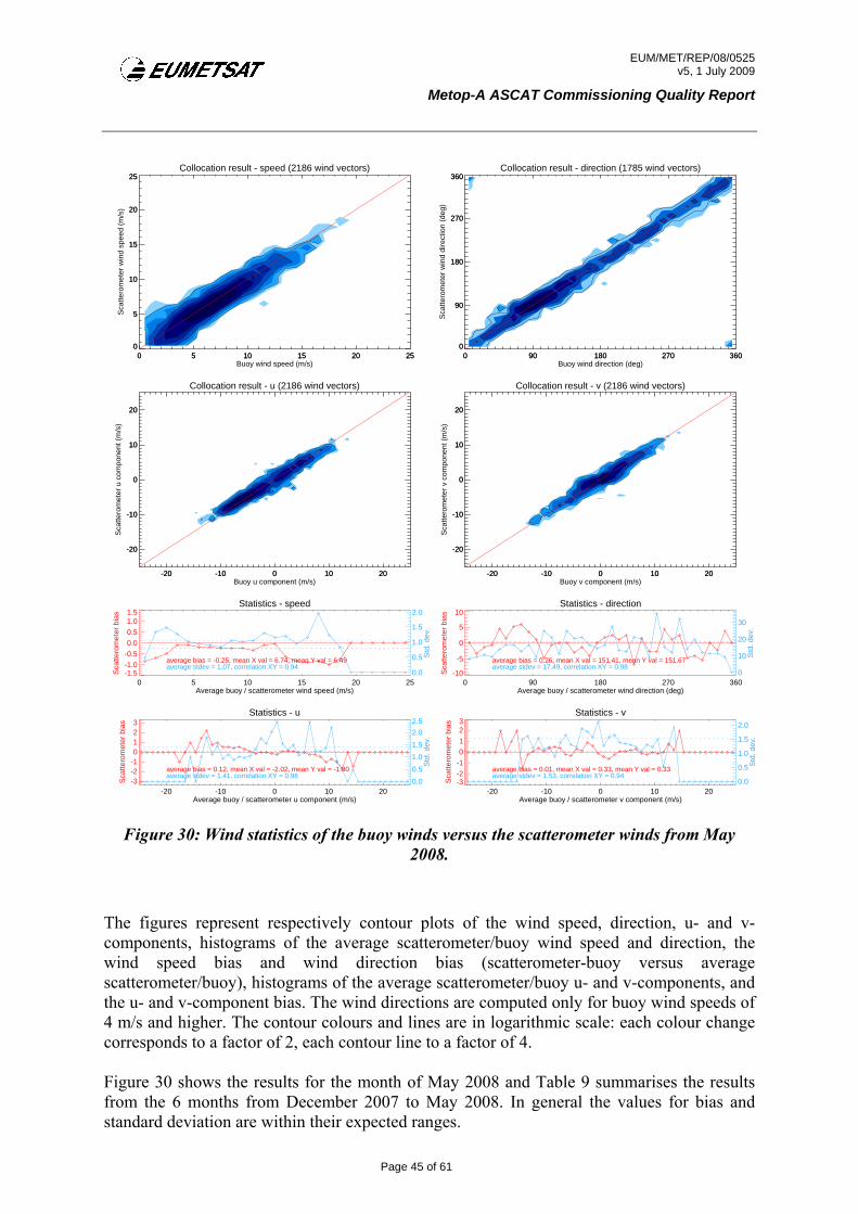
Figure 30: Wind statistics of the buoy winds versus the scatterometer winds from May 2008.
The figures represent respectively contour plots of the wind speed, direction, u- and v-components, histograms of the average scatterometer/buoy wind speed and direction, the wind speed bias and wind direction bias (scatterometer-buoy versus average scatterometer/buoy), histograms of the average scatterometer/buoy u- and v-components, and the u- and v-component bias. The wind directions are computed only for buoy wind speeds of 4 m/s and higher. The contour colours and lines are in logarithmic scale: each colour change corresponds to a factor of 2, each contour line to a factor of 4.
Figure 30 shows the results for the month of May 2008 and Table 9 summarises the results from the 6 months from December 2007 to May 2008. In general the values for bias and standard deviation are within their expected ranges.
Page 45 of 61
0.0
2.0

EUM/MET/REP/08/0525 v5, 1 July 2009
Metop-A ASCAT Commissioning Quality Report
speed bias dir SD u SD v SD December 2007 -0.01 19.67 1.79 1.96 January 2008 -0.04 19.76 1.89 1.90 February 2008 -0.07 16.62 1.95 1.89 March 2008 -0.09 17.46 1.81 1.84 April 2008 -0.15 17.94 1.71 1.69 May 2008 -0.25 17.49 1.41 1.53 Average -0.08 18.15 1.76 1.79
Table 9: Wind speed bias, wind direction standard deviation (SD) and wind component SD for ASCAT 25 km wind versus buoy data.
NB. We are grateful to Jean Bidlot of ECMWF for helping us with the buoy data retrieval and quality control.
6.3 Level 2 Flag Assessments
During level 2 wind processing various quality flags can be set to indicate suspicious or special conditions. The quality flags are encoded in the bits of the WVC quality variable (wvc_quality). In order to examine the occurrence of these flags, a table from one day of ASCAT data has been made. Table 10 shows the level 2 quality flags occurrences in 25 kmsampling mode. The data is filtered by geographical location to exclude ice contamination. Also land is filtered out making use of the L1b and L2 land flag.
The qual_sigma0 flag is set when no wind inversion is possible because of land or ice (then also respectively the land or ice flag is set) or when there is a problem with one or more of the beams: e.g. missing sigma0-values or invalid incidence angle.
The Kp flag is set when the total Kp value is above a windspeed-dependent threshold.
The knmi_qc flag is set when there is a problem found in the inversion. In most cases the distance to cone is too large, or the Kp-value is too large. Then also respectively the gmf_distance or Kp flag is set.
Quality flag Occurrence Percentage qual_sigma0 5998 1.45 Azimuth <not set> Kp 416 0.10 Monflag 0 monvalue 0 0. knmi_qc 2341 0.56 var_qc 866 0.20 land <filtered out> 0 ice 697 0.16 inversion 1954 0.47 large 0 0 small 26613 6.41 rain_fail <not set>
Page 46 of 61

EUM/MET/REP/08/0525 v5, 1 July 2009
Metop-A ASCAT Commissioning Quality Report
rain_detect <not set> no_background 1 0.00 redundant 0 0 gmf_distance 1954 0.47 Total (double counts)
40840 9.8
Total WVCs 414977 100
Table 10: Occurrence of level 2 quality flags in ASCAT 25 km sampling mode
The var_qc flag is set when variational ambiguity removal fails due to spatial inconsistency.
The ice flag is set for a sea surface temperature below -1°C.
The inversion flag is set when the inversion fails.
The small flag is set for wind speeds below 3 m/s, the large flag for wind speeds above 30 m/s.
The rain flag is not yet set.
The total count is the sum of all quality flag bits. When a particular WVC has two bits set it is counted for two.
The occurrences of flags is low for all quality-related flags. The setting of the small and large flag is largely dependent on weather conditions, so a high or low count for these flags can occur depending on weather conditions.
For the most important level 2 quality flags the dependency on WVC number is shown in Figure 31. Some flags, notably the Kp flag and the small winds flag, show a clear dependency on incidence angle, with lower number of occurrences for the inner WVCs corresponding to a low incidence angle, and higher number of occurrences towards the outer edge of the left and right swath, corresponding to a high incidence angle. Because the wind speed distribution is not dependent on the position in the swath, it is an effect of the scatterometer in combination with the level 2 processor. More measurements corresponding to low winds are rejected by the processor from the inner WVCs than from the outer WVCs. Once rejected, no wind is calculated and the WVC does not count for the low wind statistics. This results in a lower number of low wind flags for the inner WVCs.
Page 47 of 61

EUM/MET/REP/08/0525 v5, 1 July 2009
Metop-A ASCAT Commissioning Quality Report
a) b)
c) d)
e) f)
Page 48 of 61

EUM/MET/REP/08/0525 v5, 1 July 2009
Metop-A ASCAT Commissioning Quality Report
g) h)
Figure 31: Quality flag percentage as a function of WVC number. Data from 1 January 2009 is used, land and ice is filtered out.
a) qual_sigma0 (bit 22 of wvc_quality) b) Kp (bit 20)
c) var_qc (bit 16) d) ice (bit 14)
e) inversion (bit 13) f) small wind (bit 11)
g) knmi_qc (bit 17) h) gmf_distance (bit 6)
Figure 32 shows several level 2 quality parameters on a geographical map. Some quality parameters correlate with geographical location, e.g. the small-winds quality flag correlates with areas with highly variable winds, and the ice flag corresponds to high latitudes. These correlations can be explained from a physical point of view.
a) b)
Page 49 of 61

EUM/MET/REP/08/0525 v5, 1 July 2009
Metop-A ASCAT Commissioning Quality Report
c) d)
e) f)
g) h)
Figure 32: Quality flag as a function on a geographical map. Data from January 2009 is used, land and ice is filtered out.
a) qual_sigma0 (bit 22 of wvc_quality) b) Kp (bit 20)
c) var_qc (bit 16) d) ice (bit 14)
e) inversion (bit 13) f) small wind (bit 11)
g) knmi_qc (bit 17) h) gmf_distance (bit 6)
Page 50 of 61

EUM/MET/REP/08/0525 v5, 1 July 2009
Metop-A ASCAT Commissioning Quality Report
7 IMPROVEMENTS TO THE EXTERNAL CALIBRATION
7.1 Introduction
The rainforest γ0 shown in Figure 9 is generally well behaved as a function of incidence angle with the exception of beam 1, reproduced in the figure below, which shows a variation of about 0.2 dB in the lower incidence angle range. This variation is not present in the results from other beams, which suggests that it could be an artefact of the calibration process.
Figure 33: Rainforest γ0 in beam 1 as a function of incidence angle.
This issue was discussed at the 32nd meeting of the ASCAT SAG and it was recommended that the problem be investigated and solved before any reprocessing of ASCAT data takes place.
This section investigates the cause of the problem and describes a refinement to the gain model fitting in the GAPE procedure which solves it.
7.2 Distortions in the Beam Pattern
The figure below shows the transponder data and fitted gain model for beam 1. It can be seen that the transponder data shows the presence of a small distortion in the beam pattern in the region x=0.05 to 0.1, which corresponds to the near range part of the swath. It can also be seen that the fitted gain model does not accurately capture this distortion but instead is slightly too low in the centre and slightly too high at either edge.
Page 51 of 61

EUM/MET/REP/08/0525 v5, 1 July 2009
Metop-A ASCAT Commissioning Quality Report
Figure 34: Transponder data and fitted gain pattern model for beam 1.
The difference between data and model is shown in the figure below and we can clearly see an oscillation of up to 0.2 dB around the region of distortion. This implies that the variation observed in the plots of rainforest γ0 is caused by the gain model (which is used to calculate the calibration scaling factors) not accurately capturing the small distortion in the beam pattern.
Figure 35: Residual between transponder data and gain pattern model for beam 1.
Note that this distortion is not present in other beams and is thought to be a result of the position of the beam 1, mid-left, antenna which is underneath the main body of the satellite and subject to reflections from the satellite body and other instruments.
Page 52 of 61
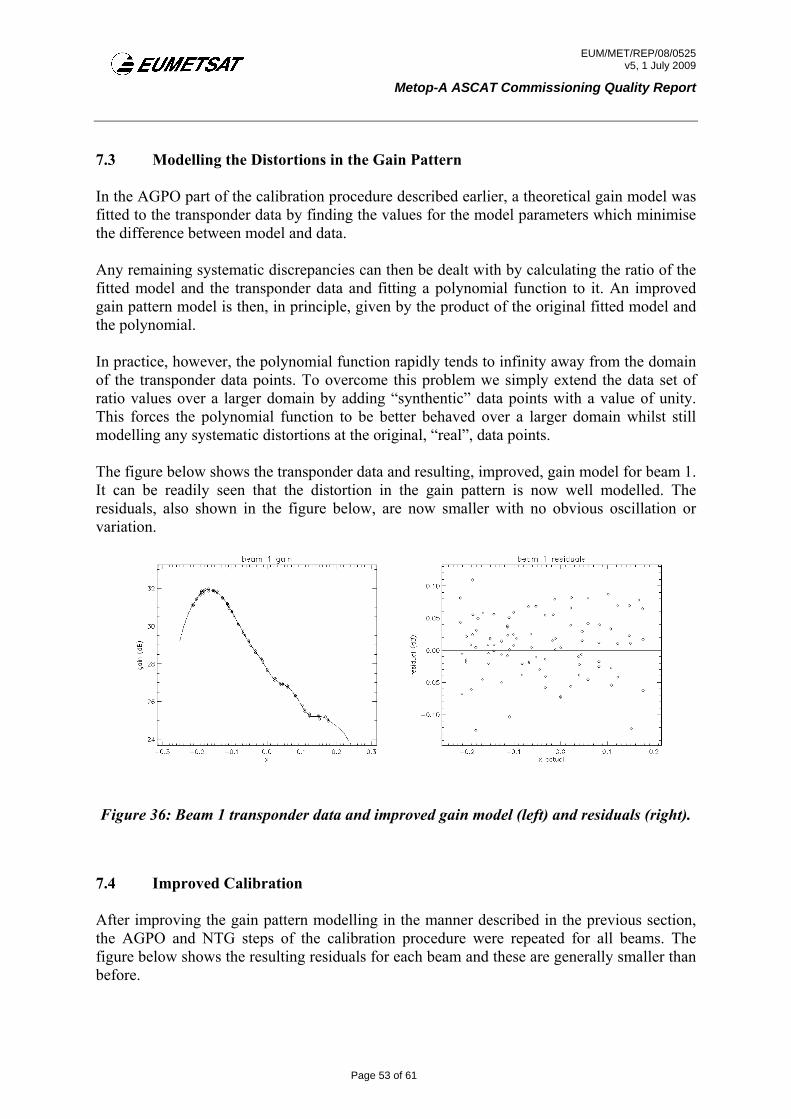
EUM/MET/REP/08/0525 v5, 1 July 2009
Metop-A ASCAT Commissioning Quality Report
7.3 Modelling the Distortions in the Gain Pattern
In the AGPO part of the calibration procedure described earlier, a theoretical gain model was fitted to the transponder data by finding the values for the model parameters which minimise the difference between model and data.
Any remaining systematic discrepancies can then be dealt with by calculating the ratio of the fitted model and the transponder data and fitting a polynomial function to it. An improved gain pattern model is then, in principle, given by the product of the original fitted model and the polynomial.
In practice, however, the polynomial function rapidly tends to infinity away from the domain of the transponder data points. To overcome this problem we simply extend the data set of ratio values over a larger domain by adding “synthentic” data points with a value of unity. This forces the polynomial function to be better behaved over a larger domain whilst still modelling any systematic distortions at the original, “real”, data points.
The figure below shows the transponder data and resulting, improved, gain model for beam 1. It can be readily seen that the distortion in the gain pattern is now well modelled. The residuals, also shown in the figure below, are now smaller with no obvious oscillation or variation.
Figure 36: Beam 1 transponder data and improved gain model (left) and residuals (right).
7.4 Improved Calibration
After improving the gain pattern modelling in the manner described in the previous section, the AGPO and NTG steps of the calibration procedure were repeated for all beams. The figure below shows the resulting residuals for each beam and these are generally smaller than before.
Page 53 of 61

EUM/MET/REP/08/0525 v5, 1 July 2009
Metop-A ASCAT Commissioning Quality Report
Figure 37: Residuals between transponder data and the improved gain models for each beam.
The improved normalisation tables were used to produce operation level 1b data from December 2008 onwards. The figures below compare the rainforest results given by the previous and the improved calibrations. As expected, the variation in beam 1 has now been removed. However, there is an indication that a smaller oscillation may now have been introduced into beam 4 at the extreme near range. This is scheduled to be investigated in more detail as during the next scheduled calibration exercise (June/July 2009).
Page 54 of 61

EUM/MET/REP/08/0525 v5, 1 July 2009
Metop-A ASCAT Commissioning Quality Report
Figure 38: Comparison of rainforest γ0 produced by the old calibration (left-hand plots) and the improved calibration (right-hand plots) for beams 0, 1 and 2.
Page 55 of 61

EUM/MET/REP/08/0525 v5, 1 July 2009
Metop-A ASCAT Commissioning Quality Report
Figure 39: Comparison of rainforest γ0 produced by the old calibration (left-hand plots) and the improved calibration (right-hand plots) for beams 3, 4, and 5.
7.5 Reprocessed Data
All ASCAT data from 2007 and 2008 was reprocessed with the improved calibration in order to produce a single consistent data set for use in ASCAT validation. The figure below compares the rainforest γ0 in each beam calculated from descending pass ASCAT data from each of these years. These results again indicate the possible presence of a minor variation in the calibration in the extreme near range of beam 4.
We also note that:
Page 56 of 61

EUM/MET/REP/08/0525 v5, 1 July 2009
Metop-A ASCAT Commissioning Quality Report
1. There is less than a 0.02 dB change between the 2007 and 2008 γ0 values which demonstrates the good temporal stability of both the rainforest test site and the ASCAT instrument,
2. The plots of γ0 are not flat, as expected, but seem to show that rainforest γ0 decreases slowly as incidence angle increases.
Figure 40: Rainforest γ0 in each beam calculated from descending pass ASCAT data from 2007 (black square symbols) and 2008 (red crosses).
Page 57 of 61

EUM/MET/REP/08/0525 v5, 1 July 2009
Metop-A ASCAT Commissioning Quality Report
8 OVERALL ASSESSMENT AND RECOMMENDATIONS
8.1 Instrument Health
Gain compression monitoring is carried out approximately every month and indicates that the instrument continues to function normally. Transmit pulse assessment and correlation between instrument telemetry and product quality have still to be performed (although we note that instrument telemetry has been analysed in [RD6]).
8.2 Internal Calibration
On-board internal calibration coefficients and receiver gain settings have been derived and applied to the ASCAT processor configuration. Receive filter shape, power gain product and noise power values have been assessed and are monitored routinely.
The power gain product is seen to vary after ASCAT switch on and during the switch on or off of other instruments on board Metop-A. The magnitude of these variations is small and is automatically compensated for during calculation of the L1b σ0 values.
Small numbers of very high noise power values are observed, mostly over land, and are believed to be the result of interference from C-band emissions coming from point sources on the ground. The effect of these high noise powers on the σ0 values is believed to be small but has still to be investigated in detail.
8.3 External Calibration
External calibration of ASCAT using all three transponders has been performed although we note that this has taken longer than originally foreseen due to problems with transponder installation and operation.
The results from a refinement to the calibration in order to remove a small ripple seen in the near range backscatter in beam 1 (left mid antenna) have also been documented.
The next calibration campaign is expected to take place in June/July 2009 and this will allow the temporal stability of ASCAT calibration to be examined and will give the opportunity to investigate and remove any small remaining calibration issues.
8.4 Level 1b Product Validation
8.4.1 Rain Forest Backscatter
Rainforest γ0 produced from ASCAT backscatter measurements have been examined and found to be close to the value expected from ERS scatterometer observations. Plots of γ0 versus incidence angle showed minor variations, less than the intended calibration accuracy, in all beams except beam 1 (left mid antenna). After the external calibration was refined, this problem was no longer present.
Page 58 of 61

EUM/MET/REP/08/0525 v5, 1 July 2009
Metop-A ASCAT Commissioning Quality Report
A preliminary comparison of rainforest γ0 values from contemporary ASCAT and ERS-2 measurements showed good agreement in two out of three beams. For the remaining beam, the γ0 values from ERS-2 were much lower than expected and this may be due to the very limited ERS coverage of the rainforest test site giving a low quantity of data and hence an unreliable estimate of γ0.
8.4.2 Sea Ice Backscatter
ASCAT backscatter over regions of stable Antarctic sea ice has been compared to an ice line model developed from ERS scatterometer data. The difference between them was found to be acceptably small in the lower incidence angle range but increased as incidence angles became larger. This is more likely to indicate a problem with the model, which has not been validated at the larger incidence angles seen by ASCAT, rather than a problem with the ASCAT calibration.
8.4.3 Ocean Backscatter
ASCAT backscatter over the open ocean has been compared to the CMOD-5 backscatter model. In common with the validation using stable sea ice, the difference between them was found to be acceptably small in the lower incidence angle range but increased as incidence angles became larger. Again, this is likely to be a problem with the model, which was developed using ERS data and has not been validated at the larger incidence angles, rather than with the ASCAT calibration.
8.4.4 Kp Assessment
Kp values have been examined and appear reasonable and on average representative of the expected instrument noise levels, i.e., less than 3%. Higher values of Kp are observed and seem to have a geographical signature indicating that they contain potentially useful information which could be used to improve wind retrievals.
8.4.5 L1b Flags
The L1b product flags produced by processor version 5.6.0 have been found to have various anomalies which make the use of the summary flag F_USABLE not possible. These are related to F_OA and F_EXT_FIL. Furthermore, F_SA also contributes to set F_USABLE to 2, while the data flag for potential solar array reflections interference is used and does not show a dramatic quality degradation. These problems have been addressed in version 5.7.0 of the processor.
The implementation of F_TEL is pending for future processor versions, as well as the validation of F_F and F_V.
Page 59 of 61

EUM/MET/REP/08/0525 v5, 1 July 2009
Metop-A ASCAT Commissioning Quality Report
8.5 Level 2 Product Validation
8.5.1 Extended Ocean Calibration
The OSI-SAF tools used at KNMI have been used to find a set of bias correction values that bring ASCAT backscatter measurements into optimum agreement with the CMOD5.n ocean backscatter model. Bias corrected ASCAT backscatter is used operationally to produce the level 2 wind product and this is found to have similar characteristics to the ERS scatterometer wind product.
Prior to each change in the calibration of the ASCAT level 1b data, the bias correction tables have been recalculated using a level 1b test data set. This has allowed the characteristics and performance of the level 2 wind product to remain stable over time and insensitive to changes in the quality of the level 1b data.
8.5.2 Buoy Comparisons
Wind statistics have been collected for a 5-month period from collocated scatterometer and buoy data. Analysis of this data shows a wind speed bias of approximately -0.1 ms-1 for ASCAT 25 km neutral winds versus buoy data and a standard deviation for wind components of approximately 1.8 ms-1.
The ASCAT wind product accuracy requirements are 2 ms-1 for the ASCAT wind vector components with respect to a “true” wind reference. Although the RMS scores do not provide a measure of the ASCAT wind accuracy alone, but rather the combined error of ASCAT and ECMWF or buoy winds, it is clear that the wind product quality meets this requirement.
8.5.3 L2 Flag Assessment
The occurrence of all level 2 quality flags has been examined and, where appropriate, their dependency on WVC number and geographical location analysed.
Qual_sigma0 and knmi_qc can be seen as the overall level 1b quality flag and the overall level 2 quality flag respectively. They have low occurrences of 1.45% and 0.56%. Work on a rain flag is ongoing.
The Kp flag and low winds flag exhibit a dependency on WVC number which can be understood from an instrument point of view as the noise and backscatter characteristics vary with incidence angle.
The low winds flag exhibits some dependency on geographical location which can be understood from a physical point of view as ocean regions that have a high wind variability are more likely to show low winds.
Page 60 of 61

EUM/MET/REP/08/0525 v5, 1 July 2009
Metop-A ASCAT Commissioning Quality Report
8.6 Recommendations
The analysis presented in this document demonstrates that the ASCAT calibration has reached a standard which meets requirements and satisfies user expectations.
Minor activities, which are not critical to the calibration or operational use of ASCAT data, remain to be completed, namely:
• validation of level 1b flags which relate to gaps in data, • further analysis to determine the effect of interference from ground sources on
ASCAT backscatter, • the analysis of instrument and platform telemetry from L1a products, and • the analysis of pulse shape and FM rate of the ASCAT transmit pulses captured by the
ground transponders. It is recommended that these activities are initiated and completed.
We also note that several papers describing the calibration and validation of ASCAT data have either been submitted for publication in peer reviewed journals or are in preparation:
• Radiometric calibration of the advanced wind scatterometer ASCAT carried on board Metop-A satellite (submitted to Trans. Geosci. & Rem. Sens.)
• ASCAT scatterometer ocean calibration (submitted to Trans. Geosci. & Rem. Sens.) • Validation of backscatter data from the advanced wind scatterometer ASCAT carried
on board Metop-A satellite (in preparation).
Page 61 of 61


