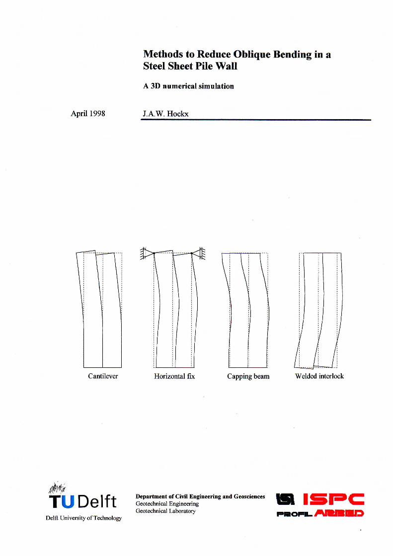
April 1998

Cantilever

Delft University of Technology

Methods to Reduce Oblique Bending in a Steel Sheet Pile Wall

A 3D numerical simulation

JA.W. Hockx

Horizontal fix Capping beam Welded interlock

Department of Civil Engineering and Geosciences • I ~ P.!!!It c: Geotechnical Engineering ~ .-GeotechnicaI Laboratory PlROPIL. AaBII!I.I:)

Methods to Reduce Oblique Bending in a Steel Sheet Pile Wall

A 3D numerical simulation

by

JAW. Hockx

Geotechnical Laboratory

Graduation committee:

Prof Ir. AF. van Tol Dr. -Ing. A Schmitt Ir. O.M. Heeres Ir. D.A. Kort Ir. K.G. Bezuyen

A graduation project carried out at:

Delft University of Technology Department of Civil Engineering

Apri11998

Foundation Engineering ISPC profilARBED Computational Mechanics Foundation Engineering Hydraulic and Geotechnical Engineering

• Hydraulic and Geotechnical Engineering Division Foundation Engineering Group

• Mechanics and Constructions Division Computational Mechanics Group

In assignment of

ISPC profilARBED Recherches

Preface

This report completes my graduation project: 'Methods fo reduce oblique bending in a steel sheet pile wall', which is the final examination of my study Civil Engineering at the Delft University of Technology.

This graduation project is carried out in co-operation with ISPC profilARBED (Luxembourg) and the Foundation Engineering and Computational Mechanics groups ofthe Department ofCivil Engineering, Delft University of Technology. I am grateful for the provided facilities and expertise which made this project possible.

I would like to express my gratitude to Dr.-Ing. A. Schmitt, Ir. D.A. Kort and Ir. O.M. Heeres for their guidance during the course ofthis project. Their comments and discussions during this project were of great value. Furthermore, I would like to thank the people who spent their time reading the concept versions ofthis report .

Delft, April 1998

Johan Hockx.

- 1 -

Summary

For over three quarters of a century steel sheet pile walls are applied in geotechnical practice. Sheet pile walls consisting of steel are usually applied when large differences in elevation must be sustained and heavy loads are acting upon the sheet pile wall. This is for example the case with quay walls and construction pits in urban surroundings.

Steel sheet pile walls usually have a wave like cross-section consisting of U- or Z-profiles. The wave like cross-section ensures favorable strength- and stiffuess properties. A common used variant is a sheet pile wall composed of so called double U-profiles. These profiles consist oftwo single U-profiles fixed in the common interlock by welding or crimping. A very specmc property ofthe double U-profile is an asymmetric cross-section which can lead to a rotation ofthe neutral axis. As aresuit ofthis , the sheet pile wall tends to deflect both forward (lateral) and sideways (transverse). Because the double U­profiles are bending in both lateral and transverse direction, this phenomenon is called oblique bending. As a result of oblique bending the strength and lateral stiffuess ofthe sheet pile wall is reduced compared to a continuous sheet pile wall.

Oblique bending goes together with slip in the free interlocks and a transverse deflection ofthe sheet pile relative to the soil body. In an earlier study, the transverse bearing capacity ofthe soil (i.e. reduction ofthe transverse displacement ofthe sheet pile by the soil) has been evaluated. In that study it is concluded that in case of a high groundwater level, the soil is not able to give a transverse restraint which significantly reduces oblique bending.

Aim ofthis graduation project is to evaluate four different methods to reduce oblique bending in a steel sheet pile wall. The four methods which have been studied are: • A steel sheet pile wall without a resulting water pressure. • A steel sheet pile wall with a fix ofthe horizontal displacement at the top . • A steel sheet pile with the sliding interlock welded during the excavation. • A steel sheet pile wall with a capping beam on top.

The main goal ofthis study is to determine which method is able to give the highest reduction of oblique bending. Therefore calculations are made with a three dimensional finite element model of a dry excavation of a soil body (a middle-dense compacted sand) in front of a cantilever sheet pile wall consisting of double U-profiles. Furthermore use is made of a perfectly rough (r5 = rf) sheet pile wall which implies no slip ofthe soil along the axis ofthe sheet pile. Also the sheet pile is modeled without a resulting water pre~sure on it. In this waya 'best case' model is obtained with which aprediction can be made what best possible result can be obtained by applying some kind ofmethod to reduce oblique bending.

First analytical calculations are made of a simply supported sheet pile with a distributed load, in order to evaluate the influence ofthe loading conditions on the bending characteristics. The loading conditions in lateral and transverse direction appeared to be of great influence on the strength and stiffuess of the sheet pile. The maximum or upper limit strength and stiffuess is derived if oblique bending is prevented by fixing the free interlocks (no in plane deformation). Depending on the loading conditions, the stiffuess varies from 0.49 to 1 time the maximum stiffuess. The strength appeared to vary from 0.59 to 1 time the maximum strength. The lower limit of the strength and stiffuess is obtained when no transverse bending moment is activated and the in plane deformation is free. The lower-limit and upper­limit is used in a 2D-finite element computation in order to determine the maximum and minimum lateral displacements.

Furthermore, 3D-finite element computations are made for the four methods to reduce oblique bending. The lateral deflections ofthe sheet pile wall in these calculations are compared to the upper- and lower-

-2-

limit deflections ofthe 2D calculations. In this waya quantification can be made ofthe magnitude that a method has on reducing oblique bending.

From the results ofthe 3D calculations, it appeared that sand is not able to give a transverse restraint which significantly reduces oblique bending under these 'best case' condition. A steel sheet pile wall with a fix ofthe horizontal displacement at the top is reducing oblique bending somewhat more. The stiffuess is increased in this case to 0.61 times the maximum stiffuess. The strength is increased in this case to 0.70 times the maximum strength.

A capping beam is a concrete casing on the sheet pile head. This concrete casing is installed after the sheet pile is driven into the ground and before the sheet pile is able to deform due to an excavation. When a capping beam is installed on top of a sheet pile wall, it is assumed that the slip in the free interlock at the sheet pile head is impeded. As aresult ofthis impediment, a transverse restraining moment is activated which reduced oblique bending considerable. The stiffuess is increased to 0.71 times the maximum stifthess and the strength is increased to 0.72 times the maximum strength.

With every new excavation step the lateral- and transverse displacements increase. As aresuit ofthe increasing transverse displacements, the slip in the interlock also increases. From the results ofthe sheet pile with a capping beam on top, it can be observed that ifthe slip in the free interlock is impeded the sheet pile acts much stiffer. As a logical follow up, the interlock ofthe sheet pile is welded after a small excavation step. In this way no further slip can develop in the welded part ofthe interlock. The procedure for welding ofthe interlock during excavation is as follows. First an excavation step is made to ensure the interlock is accessible for welding. Because an excavation step is made, there is also some slip in the interlock. When welding ofthis part ofthe interlock is completed, the next step can be excavated and is accessible for welding ofthe interlock etc. From the 3D calculations it followed that welding ofthe interlock during excavation gave the highest reduction of oblique bending. In this case the stifthess is increased to 0.82 times the maximum stiffuess and the strength is increased to 0.77 times the maximum strength.

It is striking to notice that the stiffuess ofthe sheet pile is increasing more than the strength. This is caused by the fact that strength ofthe sheet pile only depends on the cross-section ofthe sheet pile wherethe maximum value ofthe lateral (= out ofplane) bending moment occurs. In this cross-section the maximum stress occurs. The stiffuess ofthe sheet pile depends on the distribution ofthe transverse (= in plane) restraining moment over the entire sheet pile. The restraining moment in one cross-section is less subjected to variation so the strength ofthe sheet pile is also.

In order to investigate oblique bending further it is recommended to investigate other types of sheet pile constructions, such as sheet pile walls with anchors, struts or walings, have on reducing oblique bending. It can be found from the results that slip in the interlock is a very important factor for oblique bending. Therefore it is recommended to investigate the influence of friction in the sliding interlock on oblique bending.

- 3 -

Contents

Preface 1

Summary 2

1 Introduction 6 1.1 What is oblique bending 6 1.2 Aim ofthis project 8 1.3 The contents ofthe report 8

2 Analytical calculations concerning oblique bending 9 2.1 Analytical bending formulae for double U-profile 9 2.2 Material properties of modeled double PU8 profile 11 2.3 Determination ofinfluence ofloading conditions 12 2.4 Derivation ofreduction factor for moment ofinertiaI 14 2.5 Derivation ofreduction factor for section modulus W 16 2.6 Maximum admissible bending moment in sheet pile 18 2.7 Evaluation 19

3 Calculation of shear force in the interlock using a differential equation 20 3.1 General detlection equation for a simply supported double U-profile 20 3.2 Derivation of differential equation for shear force 21 3.3 Reduction of oblique bending by linear distributed shear force 21 3.4 Reduction of oblique bending by springs in the free interlock 23

4 Finite element modeling 26 4.1 Dimensions of model 26 4.2 Boundary conditions ofmodel 27 4.3 Modeling the soil 28 4.4 Modeling the sheet pile 28 4.5 Finite element mesh 28 4.6 Calculation ofbending moments and displacements 29

5 Calculations of methods to reduce oblique bending 31 5.1 Cantilever sheet pile wall with free interlocks 3 1

5.1.1 Results of 3D calculation 31 5.2 Cantilever sheet pile wall with impeded horizontal displacement at the top 34

5.2.1 Results of 3D calculation 34 5.3 Cantilever sheet pile wall with a capping beam on top 35

5.3.1 Modeling of capping beam 35 5.3.2 Results of3D calculation 36

5.4 Cantilever sheet pile wall with welded interlock during excavation 38 5.4.1 Modeling of the weId 38 5.4.2 Results of3D calculation 39

5.5 Overview of results 41

6 Different phenomena which occur in 3D calculation 50 6.1 Accuracy of displacements in calculations 50

-4-

6.2 Calculation of normal stresses in cross-section 6.3 Calculation ofthe interlock slip

7 Comparison ofreduction factors with CUR-publication

8 Conclusions and recommendations

References

52 52

56

59

61

Annex A: Analytical solution of deflection wy(x) with springs in the interlock 62 Annex B: Example of cantilever sheet pile with equalloading conditions in y- and z-direction 64 Annex C: Example of cantilever sheet pile with different loading conditions in y- and 66

z-direction

- 5 -

1 Introduction

F or over three quarters of a century steel sheet pile walls are applied in geotechnical practice. A sheet pile wall is a row of interlocking, vertical pile segments driven to form an essentially straight wall. Frequently use is made of sheet pile walls for soil and/or water retaining constructions . This means the sheet pile wall must sustain a difference in soil surf ace elevation or water elevation from one side to the other. This is accomplished by an interaction ofthe surrounding soil and the vertical pile segments.

Sheet pile walls consisting of steel are usually applied when large differences in elevation must be sustained and heavy loads are acting upon the sheet pile wall. This is for example the case with quay walls. Also in construction pits in urban surroundings, where space is limited and high demands are made with respect to deformations, steel sheet pile walls are often used.

Steel sheet pile walls usually have a wave like cross-section consisting of U- or Z-profiles. The wave like cross-section ensures favorable strength- and stiffuess properties. The U- or Z-profiles are generally driven in pairs. Sheet piles joined in pairs are connected by means ofwelding or crimping the common, rniddle interlock.

Although double U-profiles are often used with success, sometimes problems arise when the phenomenon oblique bending occurs . As a result of oblique bending the strength and lateral stiffuess of the sheet pile wall is reduced compared to a continuous sheet pile wall. This will be explained in the next paragraph.

1.1 What is oblique bending Oblique bending can occur in steel sheet pile walls which are constructed of double U-profiles. These profiles consist oftwo single U-profiles fixed in the common interlock by welding or crimping. By connecting two single U-profiles forrning one double U-profile, a new profile is created with new properties.

(a)

Wall of single U-profiles

(b)

Wall of double U-profiles

(c)

Continuous wall of fixed U-profiles

(d)

Wall of single Z-profiles

lateral

L transverse

"--Rotation of neutral axis (= oblique bending)

_._ ._ .. = Neutral axis

o = Free interlock • = Fixed interlock

Figure 1: Influence of jixing the interlock on the location of the neutral axis.

- 6-

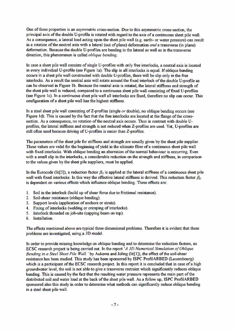
One of these properties is an asymmetric cross-section. Due to this asymmetric cross-section, the principal axis ofthe double U-profile is rotated with regard to the axis ofa continuous sheet pile wall. As a consequence, a lateralload acting upon the sheet pile wall (e.g. earth- or water pressure) can result in a rotation ofthe neutral axis with a lateral (out ofplane) defonnation and a transverse (in plane) defonnation. Because the double U-profiles are bending in the lateral as well as in the transverse direction, this phenomenon is called oblique bending.

In case a sheet pile wall consists of single U-profiles with only free interlocks, a neutral axis is located in every individual U-profile (see Figure la). The slip in all interlocks is equal. If oblique bending occurs in a sheet pile wall constructed with double U-profiles, there will be slip only in the free interlocks. As aresuit the neutral axis will rotate around the fixed interlock ofthe double U-profile as can be observed in Figure lb. Because the neutral axis is rotated, the lateral stiffhess and strength of the sheet pile wall is reduced, compared to a continuous sheet pile wall consisting of fixed U-profiles (see Figure Ic) . In a continuous sheet pile wall all interlocks are fixed, therefore no slip can occur. This configuration of a sheet pile wall has the highest stiffhess.

In a steel sheet pile wall consisting ofZ-profiles (single or double), no oblique bending occurs (see Figure Id). This is caused bythe fact that the free interlocks are located at the flange ofthe cross­section. As a consequence, no rotation ofthe neutral axis occurs. Thus in contrast with double U­profiles, the lateral stiffhess and strength is not reduced when Z-profiles are used. Yet, U-profiles are still often used because driving ofU-profiles is easierthan Z-profiles.

The parameters ofthe sheet pile for stiffhess and strength are usually given by the sheet pile supplier. These values are valid for the beginning of yield in the ultimate fibre of a continuous sheet pile wall with fixed interlocks. With oblique bending an aberration ofthe nonnal behaviour is occurring. Even with a small slip in the interlocks, a considerable reduction on the strength and stiffhess, in comparison to the values given by the sheet pile suppliers, must be applied.

In the Eurocode (lit[3]), a reduction factor f3D is applied at the lateral stiffhess of a continuous sheet pile wall with fixed interlocks. In this way the effective lateral stiffhess is derived. This reduction factor f3D is dependent on various effects which influence oblique bending. These effects are:

1. Soil in the interlock (build up of shear force due to frictional resistance). 2. Soil-shear resistance (oblique bending). 3. Support levels (application ofanchors or struts). 4. Fixing of interlocks (welding or crimping of interlocks). 5. Interlock threaded on job-site (capping beam on top). 6. Installation.

The effects mentioned above are typical three dimensional problems. Therefore it is evident that these problems are investigated, using a 3D model.

In order to provide missing knowledge on oblique bending and to determine the reduction factors, an ECSC research project is being carried out. In the report 'A 3D Numerical Simulation of Oblique Bending in a Steel Sheet Pile Wall. ' by Aukema and Joling (lit[I]), the effect ofthe soÏl-shear resistance has been studied. This study has been sponsored by ISPC ProfilARBED (Luxembourg) which is a participant ofthe ECSC research project. In this report it is concluded that in case of a high groundwater level, the soil is not able to give a transverse restraint which significantly reduces oblique bending. This is caused by the fact that the resulting water pressure represents the main part ofthe distributed soil and water load at the back ofthe sheet pile wall. As a follow up, ISPC ProfilARBED sponsored also this study in order to determine what methods can significantly reduce oblique bending in a steel sheet pile wall.

-7 -

In their study ofthe soil-shear resistance, Aukema and Joling have used the finite element system OIANA (lit[4]) to generate an appropriate 30-finite element model in which the soil is modeled elasto­plastic in combination with a correct steel sheet pile mesh. This 30-finite element model will also be used in this investigation. In this way a comparison can be made between the different effects which influence oblique bending. In this report the effects of fundamentally different methods to reduce oblique bending will be investigated.

1.2 Aim of this project Aim ofthis graduation project is to evaluate four different methods to reduce oblique bending in a steel sheet pile wall. This has been done by altering the 30-finite element model used by Aukema and Joling. The four methods which have been studied are: • A steel sheet pile wall without a resulting water pressure. • A steel sheet pile wall with a fix ofthe horizontal displacement at the top . • A steel sheet pile with the sliding interlock welded during the excavation. • A steel sheet pile wall with a capping beam on top .

In this way recommendations can be given on the reduction factors ofthe stiffhess and strength of a steel sheet pile wal!.

1.3 The contents of the report In chapter 2 analytical ca1culations are made concerning oblique bending in a double U-profile. Based on these formulae, the influence ofthe loading condition on oblique bending is evaluated. Also reduction factors for the moment of inertia and the section modulus are derived. In chapter 3 a differential equation is derived in order to calculate the shear force in the interlock. Chapter 4 deals with the finite element modeling ofthe test case. This test case is used to quantifythe reduction of oblique bending as aresuit ofthe different reduction methods. The modeling ofthe soil and the sheet pile are also discussed, as well as the dimensions and the boundary conditions ofthe test case. In chapter 5 the results ofthe 30 ca1culations are given. For every method to reduce oblique bending the reduction factors for strength and stiffhess are derived and discussed. The typical 30 phenomena that occur in the ca1culations are discussed in chapter 6. Furthermore in chapter 7 a comparison is made between the ca1culated 30 results and the normative CUR publication. Finally the general conclusions and recommendations are given in chapter 8.

- 8 -

2 Analytical calculations concerning oblique bending

The main goal in this chapter is to derive general reduction factors for the moment of inertia Rl and the section modulus Rw which take into account the phenomenon oblique bending. These reduction factors can then be applied to the material properties as given by the sheet pile supplier.

In order to derive the reduction factors for oblique bending, the analytical formulae for two directional bending have been studied. Especiallythe influence ofthe loading conditions on the bending characteristics ofthe profile have been evaluated.

2.1 Analytica! bending fonnulae for double U-profile In Figure 2 all variables for the bending formulae are de:fined along with the chosen coordinate system. The origin of coordinates is placed at the centre of gravity ofthe profile. The x-axis coincides with the fixed interlock ofthe two connected U-profiles which form the double U-profile.

The constitutive relations for two directional bending in a matrix form are (see also den Hartog, lit[6] and Verruijt, lit[lO]):

The moments of inertia with respect to y and z axes and the product of inertia with respect to the y and z axes are de:fined by the integrals:

I y'y =fy2dA A

I zz = f z 2dA

A

I yz =1 zy = f yzdA A

and the curvature by:

z

Figure 2: Definition of the coordinate system and variables in the bendingformulae for a double U-profile.

Inversion ofthis matrix gives the general equations for bending:

-lyz ][My(X)] I Y.Y M z(x)

y

The neutral axis ofthe cross-section is the line of zero stress and divides the cross-section in a part with tensile stresses and a part with compressive stresses. The angle p"'x) that the neutral axis forms with the y-axis, see Figure 3, is de:fined by the relation:

- 9-

Substituting this relation in the constitutive relation gives the following equation:

In this waythe rotation ofthe neutral axis can be determined ifthe geometrical properties ofthe profile and the applied load are known. The rotation ofthe neutral axis difIers for every specific point along the x-axis ofthe profile. Depending upon the magnitudes and directions ofthe bending moments, the angle ft may vary from -900 to +900

.

lateral

+~ z z

transverse

Figure 3: Dejinifion of the angles a, ft and r

• 0= Free interlock • = Fixed interlock

y

• y

The transverse (in plane) bending momentMy(x) and the lateral (out ofplane) bending moment Mz(x) are components ofthe resultant moment vector M . This vector forms an angle J{x) with the z-axis (see Figure 3). Therefore tanJ{x) is defined as the ratio:

M (x) tany(x)=- y

M z(x)

The direction to which the vector M is pointing, is the area where tension stresses occur. This means that a positive momentM;.. produces compression (negative stresses) on the left-hand side ofthe cross­section and tension (positive stresses) on the right-hand side. Similarly, a positive momentMz produces compression on the bottom and tension at the top, see also Figure 2.

Using Mohr's circle, we can derive the principal axes for the double U-profile and the angle a. This is the angle between the chosen coordinate system (y, z), and the coordinate system ofthe principal axes (y., z*). In Figure 4 the principal axes ofthe double U-profile are determined.

- 10 -

* z

lyz

* y

Figure 4: Mohr 's circle for the inertia properties of the double U-profile.

The y * -axis is the principal direction yielding the maximum moment of inertia 11. This is therefore the strongest axis of the profile. The z * -axis is the principal direction yielding the minimum moment of inertia 12 and is consequentlythe weakest axis ofthe profile. From Figure 4 also follows :

tan(2a) = .l (I _ I ) 2 y.y zz

Now we have defined three different angles: • a = angle of rotation of principal directions

This angle only depends on the geometry ofthe profile. • f3 = angle of rotation of the neutral axis

This angle depends on both geometrical properties and the loading conditions. • y= angle ofrotation ofresultant moment vector M (= load angle)

This angle only depends on the applied loads.

2.2 Material properties ofmodeled double PU8 profile The double U-profile used in this study is the double PU8 profile from Profil Arbed (lit[7]). This profile has been simplified in order to obtain a workable 3D sheet pile model (lit[l]) . As a consequence, the stifihess parameters ofthe modeled profile differ somewhat from the parameters which can be calculated from the geometrical dimensions ofthe real profile as given by the sheet pile supplier.

There are two different stiffuess properties: 1) Stifihess given by the supplier of the sheet pile. 2) Stifihess that has been calculated from the geometry ofthe modeled sheet pile.

The different stiffuess properties for the double PU8 profile are given in table 1.

- 11 -

Table 1: Two di ferent stiffness propertiesfor the double PU8 profile.

l zz lyy l yz

Supplier 1.3953-104 m4 1.83100-10-3 m4 -3 .3986-104 m4

Modeled pile 1.3953-104 m4 1.83143-10-3 m4 -3 .5990-104 m4

The stiffuess properties ofthe modeled sheet pile have been used in the analytical calculations.

Note that the moment of inertia l yz is negative in this case because the cross-section ofthe profile is only present in the negative second and fourth quadrant ofthe yz-plane (see Figure 3). Thus l yz is only negative because ofthe chosen coordinate system.

2.3 Detennination of influence of loading conditions It is interesting to see what the relation is between the angles a, f3 and the load angle y. With this relation we can see which is the effect ofthe loading conditions on the rotation ofthe neutral axis. The rotation of the neutral axis is of great importanee in order to derive the reduction factor Rw for the section modulus.

In subjoined figure for different loading conditions (tan f), the value for the rotation ofthe neutral axis (tan fJ) is given. Also the angle ofthe principal axes (tan a) is pictured . .

-1 lyz lyy 0

My ----l.~ tan y= - -

Uz -2 1

-1 2 ~ A lzz~

0

-0.05

~ lyz -0.1

l yy \ -0.15 tan f3

-0.2 tana~

J -0.25

-0.3

Figure 5: lnjluence of loading condition (tan rJ on the rotation of the neutral axis (tan f3) for a double PU8 profile.

It can be observed that the transverse bending moment rotates the neutral axis back to the axis of a continuous sheet pile wall. There are three significant points (A, B and C) in this figure, in which different phenomena play an important role. These three points will be discussed hereafter.

• (A) Oblique bending fully impeded If no oblique bending occurs, the angle of rotation f3(x) of the neutral axis must be zero in every point along the x-axis. This is only possible when:

So in order to fully impede oblique bending, a transverse bending moment My(x) is necessary which is a

- 12 -

factor ly/lzz= -2.58 bigger than the lateral bending moment Mix) in every cross-section ofthe profile, see also lit[8]. Note that this value only applies for this particular profile.

* z z a = -11.52° [3= 0° y=68 .81°

* y

Figure 6: Situation in case oblique bending is fully impeded.

• (B) Free oblique ben ding If free oblique bending is occurring, no transverse moment My(x) is working on the sheet pile. Thus the load angle }(x) is zero. In this case the rotation ofthe neutral axis is:

I tan[3(x) = ~ = -0.1965

lyy [3(x) = -11.17 0

So if free oblique bending occurs, the rotation of the neutral axis is equal for every cross-section along the axis ofthe profile. The rotation ofthe neutral axis [3 is somewhat smaller than the angle ofthe principal directions a .

• z z

Figure 7: Situation of free oblique bending.

a=-11.52° [3= -11.170

y=O°

• y

• (e) Neutral axis is perpendicular to the resultant moment vector M It can be found from Figure 8 that this occurs when:

tany(x) = tan[3(x)

Figure 8 shows that if [3= y, automatically y= a applies. So ifthe neutral axis is perpendicular to the loading vector M, the direction ofthis vector has to correspond with one ofthe principal directions.

- l3 -

* z z a=-11.52° {3= -11.52° y= -11.52°

~=---f---r-"'" y

* y

Figure 8: Situation when neutral axis is perpendicular to the resultant moment vector M

From Figure 5 and the three significant points in this figure it can be concluded that the loading conditions ofthe profile have a great influence on the rotation ofthe neutral axis. By altering the ratio ofthe transverse and lateral bending moment from -00 to +00, in theory every rotation angle ofthe neutral axis is possible. In the next paragraph the influence ofthe loading conditions on the reduction factors for the moment of inertia and the section modulus is derived.

2.4 Derivation of reduction factor for moment of inertia 1 When a rotation ofthe neutral axis occurs, this is an indication for oblique bending. However, the magnitude of this rotation is not an indication for the reduction factor RI of the moment of inertia. In order to derive the reduction factor RI for the moment of inertia, the maximum out of plane displacement W z at the top ofthe sheet pile has to be compared for one and two directional bending (= oblique bending).

• General dejlection curve lor one directional ben ding In case of one directional bending the following general equation is applicable:

M z(x) Kz(X)= EI

zz

The general deflection curve is obtained by a double integration ofthis equation.

wz(X)=- E~ Jf M z(x)dx2

+C]x+C2 zz

Herein, eland c 2 are constants of integration for the slope of the sheet pile and for the deflection, respectively.

• General dejlection curve lor two directional bending In case oblique bending occurs, the following general equation for bending is applicable:

Via double integration ofthis equation, we get the general deflection curve wzCx) .

wz(X)=-JfKz(x)dx2 =- E(I I I_I I )[-Iyz Jf M y(x)dx

2 +I>Y Jf M z(x)dx

2]+C3X+C4

>Y zz yz '0/

- 14 -

Again, C 3 and C4 are constants of integration for the slope of the sheet pile and for the deflection, respectively. With the ratio:

the formula for the general deflection curve becomes:

in which /;z is the apparent moment of inertia of the sheet pile defined by:

The apparent moment of inertia I ;z is defined as the moment of inertia that must be applied in a 2D

calculation in order to get the same maximum displacement at the top ofthe sheet pile as in a 3D calculation. Thus by using the apparent moment of inertia, the effects that occur in a 3D calculation can be taken into account in a 2D calculation.

Normally, the moment ofinertia is a material property and only depends on the geometry ofthe cross­section. But in case ofthe apparent moment ofinertia, it also depends on the loading condition.

The general deflection curve for two directional bending has to be compared with the general deflection curve for one directional bending to derive the reduction factor Rl for the moment of inertia. It is assumed that the boundary conditions at the beginning ofthe sheet pile (x = 0) are equal for both one and two directional bending. This imp lies that the displacement and the slope ofthe sheet pile wall at x = 0 are equal thus Cl = C3 and C2 = C4.

In case of a cantilever sheet pile wall, the deflection and the slope ofthe sheet pile wall at x = 0 are zero, see Figure 9. Thus we obtain:

qJy(O)=O

wz (O)=O

Cl = C3 =0

Cz = C4 =0 ~-=~~-CfJy ..... (X)-------'---w-z~) · · ·· · ···~ x

z ...

1

Figure 9: Boundary conditions for cantilever sheet pile wall.

Because the displacement wix = 1) at the end ofthe sheet pile wall is compared for one- and two directional bending, the double integral from the beginning (x = 0) to the end (x = 1) ofthe sheet pile wall has to be taken . The reduction factor Rl for the moment of inertia is defined as the ratio of the

apparent moment of inertia I ;z and the full moment of inertia / zz of a continuous sheet pile wall (=

highest stiffuess).

- 15 -

1

f f M y(x)dx2

with: R ___ ....:;0 ___ _

y - 1

f f M z(x)dx2

° The reduction factor Rl depends on the distribution of the transverse- and lateral bending moments over the sheet pile. For different loading conditions, the reduction factor Rl has been calculated. The results are given in Figure 10.

1

0.9

0.8 . . ••••• ~ • •••• • • • ••• ;. •• • • ••• • • - • - •• - - ~ - • • ••••••• •••••• .;- - •••• - ••• - - - •• 1 • - • - •••• - •••••••••••

0.7 · . . · . · . · .

Rl 0.6 · . · .

r 0.5

0.4

0.3

0.2

0.1

0 0 0.5 1 1 1.5 2 2.5

f f M y (x)dx2

1) _ _ _ 0,--__ _ .L 'r - 1

f f M z(x)dx2

° Figure 10: lnfluence of the loading condition Ryon the reduction factor Rl,

It can be observed that the reduction factor Rl for the moment of inertia is equal to 1 (= full moment of inertia) ifthe factor Ry = -ly/lzz = 2.58. This is the upper limit moment ofinertia. Ifthere is no transverse bending moment My(x) available to reduce oblique bending, a situation ofunrestrained oblique bending occurs. In this case the factor Ry = 0 and the reduction factor Rl for the moment of inertia is 0.49. This is the lower limit moment ofinertia.

The reduction factor Rl depends on the double integral ofthe bending moments My(x) andMz(x) . This implies that the reduction factor Rl depends on the distribution ofthe bending moments My(x) andMzCx) from the bottom ofthe sheet pile (x = 0) up to the top ofthe sheet pile (x = 1).

2.5 Derivation of reduction factor for section modulus W In contrast with the reduction factor RI for the moment of inertia, the reduction factor Rw for the section modulus W only depends on the bending moments in one particular point along the sheet pile. So ifwe want to calculate the reduction factor Rw ofthe section modulus in point a, we only need to know the bending moments My(a) andMz(a) in point x = a.

With the section modulus, the stresses in a cross-section ofthe sheet pile due to bending moments can be calculated. By comparing the occurring maximum stress in a cross-section for one- and two directional bending, we can calculate the reduction factor Rw for the section modulus .

- 16 -

• Maximum stress in cross-section for two directional bending In order to obtain the stresses in a cross-section of the sheet pile, the bending moments My and M z have to be converted to bending momentsM1 andM2 working in the principal directions y* and z* ofthe profile (Figure ll).

MI =My cos a +Mz sin a

M 2 = -My sin a + M z cosa

:1 Neutra! axis J

z z * • = Fixed interlock 0= Free interlock

y

* y

Figure 11: Situation of a cross-section in two directional bending.

The maximum stress in the cross-section for two directional bending can be found with the equation:

in which l and z# are the coordinates ofthe ultimate fibre with respect to the neutral axis, see Figure 11 . Furthermore, the y * -axis is the principal direction yielding the maximum moment of inertia 11. The z * -axis is the principal direction yielding the minimum moment of inertia h

• Maximum stress in cross-section for one directional ben ding In case of one directional bending, there is no rotation of the neutral axis . The maximum stress can be found with:

M , M zh (j =---=--

ID1IX,Z W I ref zz

Herein is h the height of one PU8 profile. This is the distance ofthe ultimate fibre with respect to the neutral axis. In this fibre the maximum stress occurs. Wref is the section modulus of a continuous sheet pile wall (= highest strength).

When two directional bending (= oblique bending) occurs, the stresses in the cross-section are bigger than when only one directional bending occurs due to the rotation ofthe neutral axis. This of course with equalloading conditions. By applying a reduction factor Rwto the reference section modulus Wref

for one directional bending, we are able to calculate the stresses for two directional bending for different loading conditions. To obtain this reduction factor, the maximum stress in case of one directional bending (jmax, z with a reduction factor Rw for the section modulus has to be equal to the maximum stress (jmax,yz in case oftwo directional bending.

-17 -

cr max,z = cr max,yz M zh = M,y # + M 2z#

l ref RW I, 12

M zh

cr max,z 1 zz Rw = -----'-- = ---::--=::....----::-crmax,yz M y # M Z # _ '_ + _ 2_

I, 12

For different loading conditions (tann, the reduction factor for the section modulus has been calculated. The results are shown in Figure 12.

1 r----,-----r----,----,,----~ ~~f

0.9

0.8

0.7 Rw 0.6

r 0.5 --- - - ~ --- --- + - - -- - - ~ - -- - - ~ -- - - - - -

I I I I

0.4

0.3

0.2

0.1

0 0 0.5 1 1.5 2 2.5

M. ----I.~ tan Y = - .-::2.

M.

Figure 12: lnfluence ofthe loading condition tanyon the reductionfactor Rw.

The kink shown by the graph of Rw, is caused by the shift of the point were the maximum stress occurs. For tan y2 0.189 the maximum stress occurs in the corner ofthe flange (point 1), see Figure 11. For tan y~ 0.189 the maximum stress occurs in the free interlock (point 2). It can be observed that the reduction factor Rw for the section modulus is equal to 1 (= reference section modulus) iftan y = -ly!Izz = 2.58. Ifthere is no transverse bending momentMy available to reduce oblique bending, a situation of unrestrained oblique bending occurs. In this case tan y= 0 and the reduction factor Rw for the section modulus is 0.59. This is the lower limit section modulus.

The reduction factor Rw depends on the ratio ofthe bending moments My andMz. This imp lies that only the bending moments My and M z in a cross-section need to be known in order to derive the reduction factor for the section modulus. This is aresuit ofthe direct relation between the stresses in a cross­section and the bending moments.

2.6 Maximum admissible bending moment in sheet pile The reduction factor Rw for the section modulus depends on the loading conditions. In the worst case, of unrestrained oblique bending for a double PU8 profile with free interlocks, the reduction factor Rw is 0.59 (see Figure 12). So the section modulus in this worst case scenario becomes ~ = Rw ~ref- Where:

W =lzz =1.3953.10-4 =99664.10-4 kN. /12 ~ . m.m h 0.l4

- 18 -

In order to ensure the strains in the sheet pile stay elastic, the applied moment on the sheet pile has to be restricted. When a high steel grade is used, the admissible stress in the sheet pile is about 375 N/mm2

.

The maximum admissible moment corresponding with this maximum stress is then:

M z•max = f y • Rw . w;.ef = 375.103 o/n,2' 0.59·9.9664 ·10-4 m3/12 m = 221 kNm/1.2 m

2.7 Evaluation In this chapter the general reduction factors for the moment of inertia RI and the section modulus Rw are derived which take into account the phenomenon oblique bending. Depending on the loading conditions, the reduction factor RI for the modeled double PU8 profile varies from 0.49 to 1. The reduction factor Rwvaries from 0.59 to l.

The reduction factor RI depends on the bending moments Mix) and Mz(x) along the entire sheet pile (from top to bottom). In contrast with the reduction factor RI, the reduction factor Rw only depends on the ratio ofthe bending moments My andMz in a cross-section. In order 10 obtain a deeper understanding ofthe derivation ofthe reduction factors two examples are worked out. In annex B an example of a cantilever sheet pile is given with equalloading conditions in both transverse and lateral direction. In annex C an example is given ofthe same sheet pile but now with different loading conditions in transverse and lateral direction. In order to derive the reduction factors RI and Rw for these examples, use is made ofthe theory presented in this chapter

From these examples it can be observed that the reduction factor Rw for the section modulus W, can be derived directly at the cross-section ofthe sheet pile where the maximum value ofthe lateral bending momentMz occurs. In this cross-section the maximum stress occurs. Because the stresses in a cross­section are directly related to the bending moments, only the bending moments My and Mz in this cross­section need to be known in order to derive the reduction factor for the section modulus. Furthermore it can be found from the examples that the rotation ofthe neutral axis is only constant along the longitudinal axis of a sheet pile ifthe loading conditions in the lateral and transverse direction are congruent. This means that the shape ofthe bending moments My(x) and Mz<x) must be equal.

- 19 -

3 Calculation of shear force in the interlock using a differential equation

In this chapter several analytical calculations conceming oblique bending in double U-profiles are made. Emphasis is put on modeling the shear force in the sliding interlocks. The results ofthe analytical solutions are evaluated by 3D-finite element computations.

3.1 General deflection equation for a simply supported double U-profile In this paragraph the deflection formulae for a simply supported sheet pile (one double PU8 profile) with a uniformly distributed load are derived. Use is made ofthe coordinate system as given in Figure 13.

1=9m b = 0.6m

0= Free interlock • = Fixed interlock

, z ...

r

Figure 13: Coordinate system used in formulae.

qz = 10 kN/m2

~---- .----.. x twz ------~

I

z

The sheet pile has a length I of9 m. The uniformly distributed load qz produces a bending momentMz

and an out ofplane displacement W z• Because free oblique bending is occurring in this case, there is also an in plane displacement wy . It can be found from the general formulae for two directional bending that the equation for the deflection curve in this particular case is:

The stiffuess properties used in these formulae are the ones for a modeled sheet pile as given in table 1. In order to impede the in plane displacement wy, an additional bending momentMy is required. This in plane bending moment can be provided by a shear force t which works along both free interlocks, see Figure 13 . In the following paragraph an expression will be presented where the shear force t is coup led to the in plane displacement wy .

- 20-

3.2 Derivation of the differential equation for shear force To schematise the sheet pile, an element with length dx has been taken and analysed as shown in Figure 14. All bending moments and the distributed shear force are drawn positive in this figure.

t ---i X M{PJ~+~ 12b~C~J~+ dV' y dx dx

Figure 14: Element of sheet pile with actingforces.

The shear force t on the top and battom face of the element can be schematised as a distributed moment my.

distributed moment:

moment equilibrium:

constitutive equation:

-My +my dx+My +dMy =0

d 2 w M y = -EI yy ---+

dx

dMy --=-m dx y

From the moment equilibrium and the constitutive equation we obtain the general differential equation ofthe shear force:

Because the profile ofthe double U-profile has an asymmetric cross-section and therefore a product of inertia lyz, the differential equation becomes:

3.3 Reduction of oblique bending by a linear distributed shear force The equation for the in plane deflection curve wix) ofthe sheet pile, produced by the uniformly distributed load qz is:

lfwe substitute this detlection curve in the differential equation derived in the previous paragraph, we obtain a distributed shear force tq(x). This shear force can be seen as a load acting on the sheet pile m the transverse y-direction.

- 21 -

I t (x)=-~q [x-1..I] q I z 2

zz

In order to impede the in plane deformation, a distributed shear force t(x) is needed that is opposite to the shear force tq(x) caused by the distributed load. In this way, the deflections caused by the distributed load qz are neutralised and no in plane deformations occurs.

tq (x) = -t(x)

Thus in order to fully impede oblique bending of a simply supported sheet pile with uniformly distributed load qz, the sheet pile has to be loaded bya linear distributed shear force t(x) as depicted in Figure 15.

• ••••• o _ ____ __ _ ___________ _ _____ _ .. __ _ ________ __ __ _ _ ___ __ _ __ ____ _ __ _ _

b

~----I~ Z x

b y

~~ t(x)

I .. Figure 15: Distribution of shear force t(x) in the free interlock.

From this figure it can be observed that the shear force has a maximum value at both ends ofthe sheet pile and decreases to zero in the middle. The shear force is positive on the left half ofthe sheet pile and negative on the right half. By integrating the formula for the shear force, we obtain the in plane bending moment Mix) that is needed to impede oblique bending.

The boundary condition at the support is My(O) = 0, which implies that Cl = 0. Thus the equation for the in plane bendingmomentMy(x) is:

M y (x) = ; z fq z[x2

-Ix]= ~YZ M z(x) zz zz

This is exactly the same formula as derived in the previous chapter. This has been tested in the 3D modelofthe sheet pile. The results are presented in the following tabie.

- 22 -

Table 2: Shearforce needed to imp, ede oblique bending.

t(x=O) [kN/m]

Analytical 116.07

Numerical 116.73

The analytical and numerical solution difIer only 0.6 %. So this theory corresponds with the values which were found numerically.

3.4 Reduction of oblique bending by springs in the free interlock By placing springs in the free sliding interlock ofthe sheet pile, a distributed shear force tspring{x) is simulated. The springs have a constant spring stiffuess k and can only deform in the x direction. The distributed shear force onlyexists ofthere is a displacement ofthe sheet pile, as shown in Figure 16. A displacement ofthe sheet pi Ie results in a slip u(x) in the sliding interlock. Because the springs are only mobilised ifthey are deformed in axial direction, a certain displacement ofthe sheet pile is necessary.

Because a certain displacement is necessary to mobilise the springs, it is evident that the springs in the interlock never can impede oblique bending fully. Only when k = 00, no oblique bending occurs. In this case of k = 00, a fixed interlock by wel ding or crimping is modeled.

~-------.---------------r----------------~----~x

2b

y

Figure 16: Principle of springs in the free interlock

From the geometry of Figure 16, we obtain the following relationship between the rotation tpz(x) and the slip in interlock u(x) .

dwy(X)} tpz(x) = dx _ _ dwy(x)

() u(x) - 2b

- ux dx tpz (x) =--v;-

The distributed shear force tspring{x) acting on the sheet pile produced by the springs, can be found by introducing the distributed spring stiffuess k [N/m2

] :

t spring (x) = -ku(x)

= 2bk dwy(x) ['%] dx

Like in paragraph 3.3, we cao assume the distributed shear force tq(x) caused by the distributed load qz as a load acting on the sheet pile. The shear force tspring{x) as derived above is the phenomenon which opposes this load. So we cao write for the differential equation of the shear force:

- 23 -

Substituting the expressions for the shear forces tix) and tspring(X) yields:

If we solve this equation for wy in x, we get the following function:

with:

Forthe derivation ofthis function, see annex A.

Ifthe distributed spring stiffuess k = 0, free oblique bending occurs with an in plane deflection curve wy(x) as given in paragraph 3.3. If k = 00 the in plane deflection wy ofthe sheet pile is zero. In this case, as mentioned before, no oblique bending will occur. With the use ofthe analytical formula for the in plane deflection with springs in the interlock, in an iterative way the distributed spring stiffuess krefhas been found where the in plane deflection at mid span (x = l/2-T) is halfthe value ofthe deflection in the situation of free oblique bending wy(l/2 T)free. This has been done in order to determine the influence of the spring stiffuess on the in plane deflection. The reference distributed spring stiffuess kref tumed out to be 1.5959-107 N/m2

. This is very high stiffuess.

For different spring stiffuesses kspring, the corresponding deflection wy(l/2-T) at mid span has been determined. This is done analytically as well as numerically.

1 0_9 - - Analytical solution

0.8 --- ---- Numerical (10 Springs)

w/t Z) 0.7 -0-- Numerical (20 Springs)

w itl)free 0.6 0.5

i 0.4 0.3 0.2 0.1

0 0 2 4 6 8 10 12 14 16

Figure 17: The transverse displacement wy at mid span as a function of the spring stiffness kspring.

From Figure 17 it can be found that the in plane displacement is decreasing rapidly for values up to 4 to

- 24-

6 times the reference value for the spring stifihess. After this, the displacements are not decreasing very fast. Furthermore it can be noticed the spring stifihess kspring has to go to infinity to completely impede the in plane displacement at mid span (modeling offixed interlock).

Also it can be observed that the numerical solution with 10 springs is closer to the analytical solution than the numerical solution with 20 springs.

- 25 -

4 Finite element modeling

In order to study the phenomenon oblique bending of a steel sheet pile wall in combination with the interaction ofthe soil, a 3D test case has been designed by Aukema and Joting (lit[I]). This test case consists of an excavation of a soil body (sand) in front of a cantilever steel sheet pile wall. The finite element computations have been carried out, using the finite element package DIANA.

4.1 Dimensions of model In order to obtain a good model, the dimensions of the soil body are such that the boundaries of the model have no effect on the behaviour ofthe sheet pile wall and vice versa. Thus ifthe boundaries would have been chosen further away from the sheet pile wall, the behaviour ofthe sheet pile wall would not have changed. In Figure 18, the dimensions are given ofthe problem that is analysed.

x = axial

y = tran~verse

Excavation dep~ I5 .0m

9.0m

:: : ' . . :: :

6.0m

1.~ Figure 18: Overview of used dimensions and dejinition of coordinate system.

All calculations in this report are made without a resulting water pressure on the sheet pile. The effective soil stresses are therefore bigger than with a resulting water pressure. This rnight have a positive effect on the transverse bearing capacity ofthe soil, i.e. the soil reduces the transverse deformation ofthe sheet pile. Furthermore a perfectly rough sheet pile (8= rjJ) is modeled. This implies equal displacements in all three directions for adjacent soil and sheet pile nodes. In this way the soil is attached to the sheet pile so that no slip can occur between the sheet pile and the soil body.

By using a perfectly rough sheet pile wall with no resulting water pressure on it, a 'best case' model is made. With the use ofthis 'best case' model, aprediction can be made ofwhat is the best possible result that can be obtained by applying some kind ofmethod to reduce oblique bending.

- 26-

4.2 Boundary conditions ofmodel The boundary conditions ofthe model are presented in Figure 19. The soil body at the front (= left) and back (= right) plane ofthe model is able to slide up- or downwards in axial direction. In lateral and transverse direction the soil body is supported. At the bottom plane the soil body is supported in all three directions. Furthermore a distributed load is present on top ofthe soil body.

axial

~ . ........... .

t ;-----'-------f ---...-+-- Excavation depth

9.0m

Llmer.d transverse

Sheet pile I5.0m

.. ~ .. 6.0m I2.0m

Figure 19: Boundary conditions of the model.

It is assumed that the sheet pile wall has an infinite length in transverse direction. In this way the effects at the end ofthe sheet pile wall are neglected, which allows to assume a periodic behaviour. One period takes up the width of one double U-profile. Because of simplicity ofthe finite element model, a volume between the fixed interlock is chosen. In Figure 20 the modeled periodic sheet pile volume is depicted with the applied boundary conditions.

v~ ! ! v~ , , () i i ()

w u~: _______ ---__ . -----_____ i w u I - . - I

i - ' - ' - - i . . I , . . I , '. ~, Modeled volume

o = Free interlock • = Fixed interlock

Figure 20: Equal boundary conditions on both sides of the periodic volume to model an infinitely long sheet pile wal/.

The boundary conditions at both ends ofthe sheet pile are equal. This implies that the displacements u, v, w and rotation () are equal. For further boundary conditions, reference is made to Aukema and Joling, lit[l] .

- 27 -

4.3 Modeling the soil The applied material properties for the sand are:

Y oung' s modulus: Poisson's ratio: density (dry): friction angle: dilatancy angle: cohesion:

E=20MPa y= 0.33 y= 18 kN/m3

fjJ= 35° If/= 5° c = 1 kPa

These material properties are realistic values for middle-dense compacted sand (see also lit[9]). As mentioned before, all calculations have been done without a resulting water pressure.

For modeling sands in the deviatoric plane, various possibilities exist. The oldest way ofmodeling sands is the Mohr-Coulomb criterion, which has proven to be an accurate description oftriaxial tests on sands. Unfortunately, in a finite element framework the stress paths are not known in advance and certainly not constant as with triaxial tests. Implementation ofthe Mohr-Coulomb criterion in a fully three-dimensional continuum poses difficulties which adheres to the multisurface character of the Mohr-Coulomb yield criterion. These problems can be avoided using a model with a continuous yield surface. Therefore the van Eekelen model has been used (lit[5]). With this relatively simp Ie model accurate predictions ofthe behaviour of sands can be obtained.

4.4 Modeling the sheet pile The sheet pile used in this study is a simplified version ofthe PU8 profile from Profil Arbed (lit[7]). This profile is simplified in order to obtain a workable 3D sheet pile model. Simplification ofthe profile is necessary because the soil elements must follow the shape ofthe sheet pile. A weIl fitting model shape ofthe sheet pile would result in too many small adjacent soil elements. The modeled sheet pile consists of eight shell elements with variabie thickness in order to obtain elastic properties similar to that of the PU8 profile. The modeled sheet pile is depicted in Figure 21 .

7.53 mm

14 cm

14 cm 32 cm 28 cm 32 cm 14 cm 4 ~4 ~4 ~4 ~4 ~

Figure 21: Dimensions ofthe modeled cross-section ofthe double PU8 profile.

The material properties ofthe simplified sheet pile model are already given in paragraph 2.2 . The elastic parameters for the sheet pile are:

Young's modulus: Poisson's ratio:

E = 2.1 -1011 Nlm2

y=0.3

Furthermore it is assumed that the sheet pile is behaving fully elastic during all calculations. In order to ensure no extreme stresses will occur, the maximum admissible bending moment in the sheet pile of 221 kNm/1.2 m as derived in paragraph 2.6 will not be exceeded.

4.5 F inite element mesh The soil mass is modeled with twenty-noded brick elements. Use is made of eight-noded shell elements to model the sheet pile. In subjoined figure, the used meshes ofthe soi! mass and the sheet pile are depicted.

- 28 -

(a) (b)

Figure 22:(a) 3D-view ofthe appliedfinite element mesh. (b) Detail ofthe sheet pile mesh.

The excavation depth in front of the sheet pile is divided in excavation steps of 0.9 m each. With every excavation step a row of soil elements with a height of 0.9 m is removed. From Figure 22 it can be noticed the soil elements are smaller near the sheet pile. This is done because we are interested in the interaction ofthe sheet pile wall with the surrounding soil. By using small elements, a more accurate model obtained in this area .

4.6 Calculation of bending moments and displacements The bending moments My and Mz are calculated by integrating all normal stresses axx over the cross­section A of the sheet pile at a certain point, multiplied by the distance y. and z· respectively (see also Figure 23). Again, the origin of coordinates is situated in the fixed interlock ofthe double U-profile.

My = f axxy*dA A

M z = t axxz·dA

z

/ ~. dA ---"

... ..... ~

b b

Figure 23: Calculation ofthe bending moments.

y

Because all stresses over the cross-section ofthe double PU8 profile are taken, a bending moment is obtained that acts per width 2b (= 1.2 m). Therefore all bending moments are presented as [kNm/1.2m].

Also the definition ofthe bending moments and rotations is given here. The moments shown in Figure 24 are drawn positive. So due to a positive bending moment Mz, there will be tension (positive stresses) along the positive z-axis and compression (negative stresses) along the negative z-axis. Similarly, a positive bending moment My produces tension along the positive y-axis and compression along the negative y-axis .

- 29-

x x

y y z z

Figure 24: Definition ofpositive bending moments and rotations.

A positive rotation qJy is defined as a rotation around the y-axis from the z-axis towards the x-axis. The other rotations are found in a similar way.

The displacements ofthe sheet pile which will be presented in the next paragraphs, are derived by taking the average displacements of all eighteen nodes in a cross-section ofthe sheet pile.

- 30-

5 Calculations of methods to reduce oblique bending

In this chapter the results ofthe 3D calculations performed with DIANA are presented. For every method to reduce oblique bending, the bending moments, the displacements and the interlock slip are presented.

The lateral displacements calculated with the 3D model are compared with the results from the 2D model. This 2D model is built up the same way as the side view ofthe 3D model (the 2D model is a ' slice ' from the 3D model). In this 2D model there are two limiting cases to model the moment of inertia ofthe sheet pile wall: • A situation in which it is assumed that oblique bending is unrestrained. This means that there is no

transverse bending moment My available to reduce oblique bending. Hence the smallest reduction factor RI forthe moment ofinertia must be used, as pictured in Figure 10. The apparent moment of

inertiaI;z that must be applied in the 2D calculation is therefore the lower limit moment ofinertia.

• A situation in which it is assumed that oblique bending in the steel sheet pile wall is fully impeded and hence the full moment of inertia of a continuous sheet pile wall is used. The reduction factor RI

is therefore equal to one. The apparent moment of inertia I ;z that must be applied in the 2D calculation is equal to the full moment of inertia and is therefore the upper limit moment of inertia.

In order to justify the assumption that these 2D calculations are the upper- and lower limit behaviour of the 3D calculations, the lateral deflection ofthe 3D calculation with fixed interlocks (full moment of inertia) should be the same as the lateral deflection ofthe upper limit 2D calculation. This assumption appeared to be correct within an accuracy of 5 %.

5.1 Cantilever sheet pile wall with free interlocks A cantilever sheet pile wall derives its support solely through interaction with the surrounding soil in which it is driven. This imp lies that no additional measures are taken to stabilise the sheet pile wall.

5.1.1 Results of 3D calculation In the presentation ofthe bending moments of all 3D calculations, reference is made to a sheet pile wall with fixed interlocks. In this waya comparison can be made between the transverse bending moment My provided by the method to reduce oblique bending and the lateral moment that is necessary to impede oblique bending.

In Figure 25 the distribution ofthe bending moments Mix) andMix) over the sheet pile are given. The maximum lateral bending moment M z peaks at a slightly lower level than the excavation depth.

- 31 -

Bending moment [kNml1.2m]

/; / ;

My (fixed) \ , / , /

/ /

/ ---/-

/ I l..

--

..... =My - = Mz

-150 -120 -90 -60 -30 0 30

0 -0.9

-l.8

-2.7

-3 .6 -4.5

-5.4

-6.3

-7.2

-8.1

-9 60 2

Interlock slip [mm]

1.5 1 0.5 o -0.5

o -0.9 -l.8

-2.7 -3.6

-4.5 Depth [m]

-5.4

-6.3

-7.2

-8.1

-9

Figure 25: Bending moments My(x) and M.(x) for a canti/ever wall after a 3.6 m excavation. Interlock slip u (x) for a cantilever wall after a 3.6 m excavation.

The transverse bending momentM;,(x) for a cantilever sheet pile wail with fixed interlocks (= oblique bending impeded) is also depicted in Figure 25. 1t can be observed that the transverse bending moment M;,(x) in case of a cantilever wail with fixed interlocks is by far greater than the one with free interlocks. This indicates that oblique bending is only reduced for a small part. The lateral bending momentM.(x) for a cantilever wail with free interlocks and a cantilever wall with fixed interlocks tumed out to be exactly the same.

In case of free oblique bending, no transverse bending moment My develops. In this case of a cantilever wall, some mechanism is providing a moment M;, which reduces oblique bending. There are three mechanisms which can provide a transverse bending moment in the sheet pile:

• transverse bearing capacity of the soil • distributed shear force in the interlock by friction • distributed shear force in the interlock by fixing (parts of) the free interlock

The free interlock ofthe sheet pile is modeled in such a waythat no friction can develop here. This means the slip in the interlock is not impeded in any way so that no distributed shear force can develop in the interlock. In this calculation no parts of the free interlock are fixed. Therefore the transverse bearing capacity ofthe soil is the only mechanism that can provide the occurring transverse bending momentMy. This moment however, is very small. To impede oblique bending fully, Mix) should be -2.58 times M.(x) in every point along the sheet pile axis as can be observed in Figure 25 .

1t is observed that the largest slip appeared at the top ofthe sheet pile and is onlyabout 1.5 mm for this excavation depth. Because the magnitude ofthe slip is very smail, the interlock slip is in practice not perceptible. Because there is a slip in the interlock, there also will be a transverse displacement ofthe sheet pile alongside the lateral displacement (= oblique bending).

The lateral displacements ofthe sheet pile wail which have been calculated for the three-dimensional case as weil for both two-dimensionallimit cases are displayed in Figure 26.

- 32 -

Lateral displacement [mm]

= 2D upper limit =3D = 2D lower limit

-40 -35 -30 -25 -20 -15 -10 -5 0

0

-0.9

-1.8

-2.7

-3 .6

-4.5

-5.4

-6.3

-7.2

-8.1

-9 -5

Transverse displacement [mm] 0

-0.9

-1.8

-2 .7

-3 .6

-4.5 Depth [m]

-5.4

-6.3

-7.2

-8.1

-9 -4 -3 -2 -1 0

Figure 26: Lateral displacement wlx) and transverse dis placement wy(x) lor a canti lever wall after a 3.6 m excavation.

Both lateral and transverse displacements in the sheet pile are negative which means the sheet pile is respectively bending towards the front- and left side, see also Figure 18 .

Aukema and Joling (lit[l]) found that the soil with a resulting water pressure on the sheet pile wall was not able to give a transverse restraint which significantly reduces oblique bending. The results ofthis 30 calculation show that without a resulting water pressure on the sheet pile wall, there is some transverse bearing capacity ofthe soil. However this transverse bearing capacity is still rather smalI. The lateral displacement at the top ofthe sheet pile wall calculated with the three-dimensional model is still very close to the two-dimensionallower limit case.

Although the slip at the top ofthe sheet pile is very small (1.6 mm), the lateral displacement at the top increased with 68 % compared to a continuous sheet pile wall with fixed interlocks .

In order to obtain the apparent moment of inertia which can be applied in a 20 calculation, the reduction factor RI for the moment of inertia must be derived. In theory, the reduction factor Rl can be derived from the transverse and lateral bending moments ofthe 30 calculation using the theory presented in paragraph 2.4. However, in order to do so the double integral ofboth transverse and lateral bending moments must be calculated. In practice, these calculated double integrals were not accurate enough which resulted in wrong reduction factors Rl for the moment of inertia. As aresult, the reduction factor RI which can be found with Figure 10 is not applicable when results from the 30 calculations are used.

In order to derive the reduction factor RI, a 10 calculation is made with the spring model MSHEET. This has been done for two reasons. • Results from MSHEET can be obtained quickly compared to results from the 20 model in OIANA. • The spring model MSHEET is often used in Outch design practice of sheet pile walls .

The procedure for obtaining the reduction factor is as follows . FITst the detlection for a cantilever sheet pile wall with fixed interlocks (= full moment ofinertia) is calculated. Then, in an iterative way, the moment of inertia of the sheet pile wall is reduced until the detlection at the top is equal to the detlection as calculated with the 30 model. The applied reduction on the moment of inertia is therefore the reduction factor RI for the moment of inertia. In this case of a cantilever wall with free interlocks, the reduction factor for the moment of inertia tumed out to be RI = 0.53 .

The reduction factor for the section modulus also depends on the loading condition ofthe sheet pile wall. But now we only have to look at the cross-section of the maximum lateral bending moment M z and corresponding transverse bending moment My. This is because the stresses in the cross-section are directly related to the bending moments. In paragraph 2 .5 the reduction factor for the section modulus Rw is given as a function ofthe bending moments My andMz• From Figure 25 and Figure 12 it can be

- 33 -

observed that:

M z =50kNm } M y =-14kNm

M --y =0.28

M z

Rw =0.64

The reduction factor for the section modulus is somewhat increased, compared to the situation of unrestrained oblique bending. In this situation the reduction factor for the section modulus is Rw = 0.59.

5.2 Cantilever sheet pile wall with impeded horizontal displacement at the top One way to reduce the oblique bending in a sheet pile wall is to impede the transverse displacements at the top of the sheet pile. Because only the transverse displacement at the top is impeded, slip in the free interlocks is still possible.

5.2.1 Results of 3D calculation For an excavation depth of3 .6 m the bending moments My(x) andMz(x) are presented in Figure 27.

Bending moment [kNm/1.2m] Interlock slip [mm] 0 0

/ J -0.9 -0.9 My (fixed) \_/~));/ -1.8 -1.8

-2.7 -2.7 ----- : r -3 .6 -3 .6 /'

I l.. -4.5 -4.5 Depth [m]

- -5.4 -5.4 -'::--- -6.3 -6.3

····· = My -7.2 -7.2

- = Mz -8.1 -8.1

-9 -9 -150 -120 -90 -60 -30 0 30 60 1 0.8 0.6 0.4 0.2 0 -0.2 -0.4

Figure 27: Bending moments My(x) andM.(x) and interlock slip u(x) after a 3.6 m excavationfor a sheet pile wal! with impeded horizontal displacement at the top.

The transverse bending momentMy(x) initiated by the transverse impediment is greater than the transverse bending moment produced bythe transverse bearing capacity ofthe soil (see Figure 25). But still the transverse bending moment My(x) initiated by the transverse impediment is much smaller than the My(x) which is needed to impede oblique bending. The slip in the interlock however, is reduced by almost 50 % compared to the slip in the cantilever wall with free interlocks.

For an excavation depth of 3.6 m the lateral displacements wz(x) and the transverse displacements wy(x) are presented in Figure 28.

- 34-

Lateral displacement [mm]

= 2D upper limit =3D = 2D lower limit

-40 -35 -30 -25 -20 -15 -10 -5 0

0

-0.9

-1.8

-2 .7

-3 .6

-4.5

-5.4

-6.3

-7.2

-8.1

-9

Transverse displacement [mm] 0

-0.9

-l.8

-2 .7

-3 .6

-4.5 Depth [m] -5.4

-6.3

-7.2

-8.1

-9 -0.5 0 0.5

Figure 28: Displacements curves w.(x) and wy(x) for an excavation of 3.6 for a sheet pile wal! with impeded horizontal displacement at the top.

It can be noted that the transverse displacement wy(x) ofthe sheet pile is now positive as aresult ofthe horizontal impediment at the top . The horizontal impediment at the top is forcing the whole sheet pile to the right.

In order to derive the reduction factor Rl for the moment of inertia, again aID calculation is made with MSHEET. In the case of a cantilever wall with a fix ofthe transverse displacement at the top, the reduction factor for the moment of inertia Rl = 0.61 .

The reduction factor for the section modulus is determined by the maximum lateral bending moment M z and corresponding transverse bending momentMy. From Figure 27 and Figure 12 it can be found that:

M z = 50kNm } M y =-43kNm

M y --=0.86

M z

Rw =0.70

Because the transverse bending moment My in the cross-section of the maximum lateral bending momentM. increased, the reduction factor forthe section modulus increased also.

5.3 Cantilever sheet pile wall with a capping beam on top A capping beam is a concrete casing on the sheet pile head. This concrete casing is installed after the sheet pile is driven into the ground and before the sheet pile is able to deform due to an excavation. When a capping beam is installed on top of a sheet pile wall, it is assumed that the slip in the interlock at the sheet pile head is impeded. For this reason the sheet pile head must be embedded adequately in the capping beam in order to absorb the shear forces which occur due to this restriction.

5.3.1 Modeling of capping beam The capping beam is modeled with the use of 'tyings' . This is a kind of 'virtual modeling', because no use is made of real elements to model the capping beam. Only the restrictions that a capping beam imposes upon the sheet pile have been implemented. Thus the slip in the interlock at the sheet pile head is impeded.

The rotation cp. around the z-axis is only impeded on top ofthe sheet pile (see Figure 29). This is done by tying the interlock nodes ofthe upper sheet pile element in the x-direction. In this way no slip will occur between the two top interlock nodes. The rest ofthe upper sheet pile nodes are tied in the y- and z-direction. Bythis, all relative displacements ofthetop nodes in the z- and y-direction are zero for adjacent interlock nodes.

- 35 -

z

x cpz = 0 x

Figure 29: Principle ofmodeling the capping beam; onlya rotation ({Jy about the y-axis is possible.

The profile isn't able to deform intemally. Only all nodes ofthe top extremity ofthe sheet pile as a whole can translate in the z and y direction. So the only degree offreedom for rotation at the top ofthe sheet pile is the rotation ({Jy around the y-axis.

5.3.2 Results of 3D calculation For an excavation depth of3.6 m the bending momentsM;,(x) andMzCx) are presented in Figure 30. If we compare the lateral bending moment Mz(x) after a 3.6 m excavation with the corresponding result from the cantilever wall (Figure 25), it is noticed that this bending moment is exactly the same. The installation ofthe capping beam has therefore no effect on the lateralload upon the face ofthe sheet pile.

Bending moment [kNm/l.2m]

My (fixed) ~ )/~/

--'" -- ;

--- , ---:.. ..

, ,

.... , ~ ..... _-

···· · = My - = Mz

-150 -120 -90 -60 -30 0 30

0

-0.9

-1.8

-2.7

-3.6

-4.5

-5.4

-6.3

-7.2

-8.1

-9 60

Interlock slip [mm]

0.8 0.6 0.4 0.2 0 -0.2 -0.4

o -0.9

-1.8

-2.7

-3 .6

-4.5 Depth [m]

-5.4

-6.3

-7.2

-8.1

-9

Figure 30: Bending moments My(x) and Mix) and interlock slip u(x) after a 3.6 m excavation for a sheet pile wal! with capping beam on the sheet pile head.

Because the rotation cpz of the sheet pile is prevented, an additional transverse bending moment M;, has developed at the top of the sheet pile. This bending moment must be absorbed by the capping beam. The transverse bending moment M;,(x) initiated by the capping beam is by far greater than that produced by the transverse bearing capacity ofthe soil (see Figure 25). But still the transverse bending moment My(x) initiated by the capping beam is smaller than the M;,(x) which is needed to impede

- 36-

oblique bending.

It is striking to see that the transverse bending momentMy(x) in the capping beam and the top part of the sheet pile is equal to the lateral bending moment Mz(x) at the excavation depth. At the point in the sheet pile where the maximum lateral bending momentM;,(x) appears, the slip in the interlock is zero (see Figure 30).

For an excavation depth of3.6 m the displacements wy(x) and wz(x) are presented in Figure 31.

Lateral displacement [mm]

= 2D upper limit --- =3D

= 2D lower limit

-40 -35 -30 -25 -20 -15 -10 -5 0

0

-0.9

-1.8

-2.7

-3 .6

-4.5

-5.4

-6.3

-7.2

-8.1

-9

Transverse displacement [mm]

-2 -1.5 -1 -0.5 0 0.5

o -0.9

-1.8

-2.7

-3 .6

-4.5 Depth [ml -5.4

-6.3

-7.2

-8.1

-9

Figure 31: Displacements curves wz(x) and wy(x) for an excavation of 3.6 for a sheet pile wall with a capping beam on the sheet pile head.

The lateral displacement at the top ofthe sheet pile wan with a capping beam is now closer to the 2D upper limit of a continuous sheet pile wan with fixed interlocks. The lateral displacement is now only 31 % bigger. So by installing a capping beam, a significant reduction ofthe lateral displacements is achieved.

In order to derive the reduction factor RI, again a 1D calculation is made with MSHEET equal to that for the previous methods. In the case of a cantilever wan with a capping beam on the sheet pile head, the reduction factor for the moment of inertia RI = 0.71 .

The reduction factor for the section modulus again is determined by the maximum lateral bending momentMz and corresponding transverse bending momentMy. From Figure 30 and Figure 12 it can be found that:

M z = 50lcNm } M y =-50lcNm

M y --= 1.00

M z

Rw =0.72

The reduction factor RI for the moment of inertia increased with 0.1 compared to the situation with an impediment ofthe horizontal displacement at the top . However, the reduction factor Rw for the section modulus only increased with 0.02. This can be explained by the fact that the reduction factor RI for the moment of inertia depends on the distribution of the bending moments over the whole sheet pile. On the contrary, the reduction factor Rw for the section modulus depends on the transverse bending moment My in the cross-section ofthe maximum lateral bending momentMz. The transverse bending moment did not increased much in this cross-section and therefore the reduction factor did not either.

The slip in the interlock in the adjacent nodes on top ofthe sheet pile is impeded by the capping beam. This means that the maximum slip in the interlock is reduced compared to that ofthe cantilever wan (see Figure 32). Furthermore the place ofmaximum slip is shifted downwards.

- 37 -

Interlock slip [mm] 0

-0.9

-l.8

-2.7

-3 .6

-4.5 Depth [m]

-5 .4

-6.3

-7.2

-8.1 -9

2 1.6 1.2 0.8 0.4 0 -0.4 -0.8

Figure 32: Slip in the interlock for the excavation depths 2.7 m, 3.6 mand 4. 5 m for a sheet pile wall with a capping beam on the sheet pile head.

During the excavation ofthe soil in front ofthe sheet pile wall, the place of zero slip shifted downwards. This is caused by the increase of lateralload upon the sheet pile with every new excavation step. For deeper excavations, the slip at the bottom ofthe sheet pile isn't zero any more.

5.4 Cantilever sheet pile wall with welded interlock during excavation From the results ofthe sheet pile with a capping beam on top, it can be observed that ifthe slip in the free interlock is impeded the sheet pile acts much stiffer. As a logical follow up, the interlock ofthe sheet pile is welded after every excavation step of 0.9 m. In this way no further slip can develop in the welded part of the interlock.

5.4.1 Modeling of the weId With everynew excavation step of 0.9 m, the lateral- and transverse displacements increase. As aresuit ofthe increasing transverse displacements, the slip in the interlock also increases, see Figure 33 .

axial

----k:1~

transverse ---

o • =nodes

Figure 33: Slip in the interlock due to in plane (= transverse) displacement of sheet pile.

- 38 -

The procedure for welding ofthe interlock during excavation is as follows . First an excavation step of 0.9 m (= the height of one soil element) is made to ensure the interlock is accessible for welding. Because an excavation step is made, there is also some slip in the interlock. When welding ofthis part ofthe interlock is completed, the next step of 0.9 m can be excavated and is accessible for welding of the interlock etc.

At first an attempt was made to model the weId in the interlock by means of 'tyings'. In this case, the corresponding nodes oftwo adjacent interlock elements have to be tied in the axial direction in order to prevent further sliding. However, DIANA didn 't support the tying oftwo nodes which already have different displacements . Therefore the weId in the interlock is modeled with a simple truss element between two adjacent nodes of the sliding interlock, see Figure 34. The truss element can only deform in the axial direction, there is neither bending nor shear deformation.

x ...--I--Node

__ --+-- Truss elément

'-L-__ Sheet pile element

Figure 34: Model ofthe weid in the interlock.

The stiffhess ofthis truss element is much greater than that ofthe sheet pile. This is necessary to ensure the axial deformation ofthe truss element is insignificant compared to the slip in the interlock. On the other hand, the difference in stiffhess between the truss element and the sheet pile elements cannot be too great in order to prevent inaccurate solutions. After several tests, the following material properties ofthe truss element met the desired requirements:

Young's modulus: Cross-section:

E= l.0·1014 Nlm2

A = 0.25 m2

5.4.2 Results of 3D calculation

(::::: 480 times stiffer than a sheet pile element)

For an excavation depth of 4.5 m the bending moments My(x) andMz<x) are presented in Figure 35. Again the lateral bending is equal to the previous cases. The transverse bending moment of course is different, due to the application ofthe truss elements. In contrast with the capping beam, the weId in the interlock is not initiating a transverse bending moment at the top of the sheet pile but rather in the middle. Also the maximum value ofthis moment is bigger than with the capping beam.

- 39-

Bending moment [kNml1 .2m]

· .... =My - =Mz

-280 -200 -120 -40 40

o -0.9

-1.8

-2.7

-3.6

-4.5

-5.4

-6.3

-7.2

-8.1

-9 120 0.2 0

Interlock slip [mm] 0

-0.9

-1.8

-2.7

-3.6

-4.5 Depth [m]

-5.4

-6.3

-7.2

-8.1

-9 -0.2 -0.4 -0.6 -0.8 -1

Figure 35: Bending moments My(x) and Mix) and interlock slip u(x) for an excavation depth of 4.5 m for a sheet pile wal! with a welded interlock during excavation.

Because an excavation is made with a depth of 4.5 m, there was only space for four truss elements of 0.9 m which reached a depth of 3.6 m. It can be observed that over this depth of 3.6 m the transverse bending moment My(x) is almost equal to the transverse bending moment which is necessary to impede oblique bending. This is an indication that oblique bending is significantly reduced.

The slip in the upper half ofthe sheet pile is almost zero. Due to the application of a truss element after every excavation step of 0.9 m, the slip is not able to fully develop here. The slip in the lower half of the sheet pile has the same shape as the previous two cases. Because a truss element only connects the top and bottom node oftwo sheet pile elements (see Figure 34), the displacement ofthe middle node is bigger. This explains the irregular distribution ofthe interlock slip in the area where truss elements are app lied.

For an excavation depth of 4.5 m the displacements wy(x) and wz(x) are presented in Figure 36.

Lateral displacement [mm]

= 2D upper limit =3D = 2D lower limit

-40 -35 -30 -25 ~20 -15 -10 -5 0

0

-0.9

-l.8

-2.7

-3 .6

-4.5

-5.4

-6.3

-7.2

-8.1

-9

Transverse displacement [mm]

-1 -0.5 0 0.5 1.5 2

o -0.9

-l.8

-2.7

-3.6

-4.5 Depth [m]

-5.4

-6.3

-7.2

-8.1

-9

Figure 36: Displacement curves wz(x) and wy(x) after an excavation of 4.5 m for a sheet pile wal! with welded interlock during excavation.

It is striking to notice that the transverse displacement wy at the sheet pile top is positive in this case, whereas in all other cases the transverse displacement are negative. The explanation for this is that hardly any positive slip could be developed in the sheet pile due to the application ofthe truss elements . Furthermore a negative transverse displacement causes a positive slip (see Figure 16). In case ofthe

- 40-

cantilever wall and the wall with the capping beam, the maximum positive slip in the sheet pile is bigger than the maximum negative slip . So aresuiting negative transverse displacement follows .

The lateral displacement at the top ofthe sheet pile wall with a capping beam is now almost equal to the 2D upper limit of a continuous sheet pile wall with fixed interlocks. The lateral displacement is now only 17 % bigger compared to a continuous sheet pile wall . So welding ofthe interlock almost completely impedes oblique bending.

The reduction factor RI for the moment of inertia is detennined with the use of MSHEET and has the value RI = 0.82.

The reduction factor for the section modulus again is detennined by the maximum lateral bending momentMz and corresponding transverse bending momentMy. From Figure 35 and Figure 12 it can be found that:

M z =100kNm }

M y =-147 kNm

M y - - =1.47

M z

Rw =0.77

The reduction factor Rw has increased again on account ofthe increased transverse bending moment My.

5.5 Overview of results In Figure 37, the transverse bending moments and lateral displacements of all methods to reduce oblique bending are presented.

Bending moment [kNm/1 .2m]

0

-0.9

-1.8

-2.7

-3.6

-4.5

-5.4

-6.3

-7.2

-8.1

-9 -150 -120 -90 -60 -30 0 30 60

Lateral displacement [mm]

1

1 Free oblique bending 2 Cantilever 3 Horizontal fix 4 Capping beam 5 Welded interlock 6 No oblique bending

-40 -35 -30 -25 -20 -15 -10 -5

0

-0.9

-l.8

-2.7

-3.6

-4 .5 Depth [m]

-5.4

-6.3

-7.2

-8.1

-9 0

Figure 37: Bending moments My(x) and lateral displacement curves wlx) for all calculated cases after an excavation of 3.6 m.

Ifwe compare the distribution ofthe transverse bending moments over the sheet pile, it is clear that a bigger, negative transverse bending moment is reducing oblique bending more. The maximum displacement at the top, and therefore also the reduction factor RI, depends on the double integral ofthe bending moments My(x) and Mz(x) as mentioned in paragraph 2.4. Therefore the shape ofthe transverse bending moment distribution has little influence on the maximum displacement.

The reduction factor Rw for the section modulus W only depends on the maximum lateral bending momentMz along with the transverse bending momentMy present in that particular cross-section. Therefore the shape of the transverse bending moment distribution has a great influence on the reduction factor for the section modulus. In table 3 all derived reduction factors are presented.

- 41 -

Table 3: Reductionfactorsfor oblique bending RI Rw

Free oblique bending (M. = 0) 0.59 0.49 Cantilever (free interlock) 0.64 0.53 Horizontal fix 0.70 0.61 Capping beam 0.72 0.71 Welded interlock 0.77 0.82 No oblique bending 1 1

In the following figure, a sketch ofthe deformed sheet pile for the four analysed cases is given. Note that this a sketch, therefore the displacements are not proportional.

axial

L transverse

--- = Oeformed sheet pile = Undeformed sheet pile

Cantilever Horizontal fix Capping beam Welded interlock

Figure 38: Sketch oJ the deJormed sheet pile in transverse direction Jor the Jour calculated cases.

If we compare the sheet pile with the horizontal fix at the top with the cantilever sheet pile it is observed that the whole sheet pile has moved because ofthe horizontal fix. However, a slip in the free interlock still occurs. As mentioned before, installation of a capping beam impedes a rotation at the top ofthe sheet pile. As aresult no slip can develop at this point. Because little slip can develop in the upper half ofthe sheet pile with the welded interlock, the sheet pile is nearly straight in this area.

In Figure 39 and Figure 40 the plots ofthe 30 sheet pile after a 3.6 m excavation are depicted for respectivelya cantilever sheet pile wall and a cantilever sheet pile wall with an horizontal fix at the top. These plots show the deformed mesh (scaled up 50 times) along with the axial stresses O"xx due to the bending moments. It can be observed the stress in the free (i.e. middle) interlock is not zero. This clearly indicates oblique bending because the neutral axis (zero stress) is rotated. occurs. The maximum stresses in the sheet pile with an horizontal fix at the top are smaller than the stresses in the cantilever sheet pile. This is aresuit ofthe transverse bending moment My(x) . Also it can be noticed from Figure 40, the sheet pile deforms intemally at the top due to the horizontal restraint.

In Figure 41 and Figure 42 the plots ofthe 30 sheet pile after a 4.5 m excavation are shown for respectively a cantilever sheet pile wall with a capping beam on top and a sheet pile wall with a welded interlock during excavation. These plots show the deformed mesh (scaled up 25 times) along with the axial stresses O"xx due to the bending moments. It can be observed from Figure 40 that the stresses in the free (i .e. middle) interlock in the top half ofthe sheet pile are considerably big. This is caused by the

- 42 -

transverse bending moment Mix) initiated by the capping beam.

In Figure 43 the vertical (axial) soil stresses 0'= and horizontal (lateral) soil stresses O'zz for a cantilever sheet pile wall after a 3.6 m excavation are pictured. As aresuit ofthe excavation, the vertical soil stresses in front ofthe sheet pile wall increases. Directly behind the sheet pile wall the soil caves in which results in an unloading ofthe vertical stresses. It can be observed that there is a distributed load of 10 kN/m2 present at the top ofthe soil body. Behind the sheet pile wall there is an unloading ofthe soil which results in a decrease ofthe horizontal soil stresses. In contrast with this, the horizontal soil stresses in front ofthe sheet pile wall are rather high. Both effect are caused by the deflection ofthe sheet pile wal1.

In Figure 44 the transverse displacement contours wy and lateral displacement contours W z are depicted on the deformed mesh of a cantilever sheet pile wall after a 3.6 m excavation. De deformed mesh is scaled up 10 times. As can be noticed the transverse displacements wy only occur directly behind the sheet pile wal1. The lateral displacements W z cover a much larger area ofthe mesh. Especially at the toe ofthe sheet pile there is some increase ofthe lateral displacements.

In Figure 45 the vertical (axial) soil stresses 0'= and horizontal (lateral) soil stresses Oiz for a cantilever sheet pile wall with a capping beam on top after a 4.5 m excavation are pictured. Here the same effects occur as with the cantilever sheet pile wall. Because the excavation depth is now 4.5 m the soil stresses are a little bigger.

In Figure 46 the transverse displacement contours wy and lateral displacement contours W z are depicted on the deformed mesh of a cantilever sheet pile wall with a capping beam on top after a 4.5 m excavation. De deformed mesh is scaled up 5 times. As aresuit ofinstallation ofthe capping beam the displacements cover a much smaller area ofthe mesh than without a capping beam.

In all plots ofthe soil stresses, the three columns of elements at the right ofthe mesh always have horizontal contour lines. This implies no variation in stresses occurs. From this it can be concluded that these elements are not necessary to model the sheet pile in the sand. However this only applies with these excavation depth up to 4.5 m. For deeper excavation, the three columns can be useful because with deeper excavations larger stresses are generated.

- 43 -

x x l:z

y

(a)

Sigma xx 77.67 66.02 54.37 42.72 31.07 19.42 7.77

-3.88 -15.53 -27.18 -38.83 -50.48 -62.13 -73.78 -85.43

Figure 39: Deformed meshes of a canti lever sheet pile wall with free interlocks with tensile- (positive) and compressive (negative) stresses O"n- [Nlmm2j due to the occurring bending moments My('x) and Mix) afteran excavation of3.6 m. (a) Front view ofthe sheet pile with transverse deformation. (b) 3D-view with both transverse- and lateral deformations (deformations scaled up 50 times).

x x l:z

y zL y

(a) (b)

Sigma xx 67.60 57.79 47.97 38.16 28.35 18.53 8.72

-1.09 -10.91 -20.72 -30.54 -40.35 -50.16 -59.98 -69.79

Figure 40: Deformed meshes of a canti/ever sheet pile wal! with an horizont al fix at the top with tensile- (positive) and compressive (negative) stresses 0'.0: [Nlmm2j due to the occurring bending moments My(x) and Mz{x) after an excavation of 3.6 m. (a) Front view ofthe sheet pile with transverse deformation. (b) 3D-view with both transverse- and la/eral deformations (deformations scaled up 50 times).

- 44-

(a)

11 r ' ! I ,

l ht .:. I 'II~ ; 11"\

11 \

": \ I. J

: 1111

'

I ... ~ r "il 1\' -'

x

tez

y

(b)

Sigma xx 135.30 114.19 93.08 71.98 50.87 29.76

8.65 -12.45 -33.56 -54.67 -75.78 -96.88

-117.99 -139.10

Figure 41 : Deformed meshes of a canti/ever sheet pile wall with a capping beam on top with tensile­(positive) and compresstve (negative) stresses 0".0; [N/mm2

} due to the occurring bending moments My(x) and Mix) after an excavation of 4.5 m. (a) Front view of the sheet pile with transverse deformation. (b) 3D-View with both transverse- and lateral deformations (deformations scaled up 25 times).

x x tez

y

(a) (b)

xx 120.73 101.94 83.15 64.36 45.57 26.78 7.99

-10.79 -29.58 -48.37 -67.16 -85.95

-104.74 -123.53

Figure 42: Deformed meshes of a cantilever sheet pile wall with welded interlocks during excavation with tensile- (positive) and compressive (negative) stresses O"n [N/mm2

} due fo the occurring bending moments My(.'C) and M:(x) after an excavation of 4.5 m. (a) Front View of the sheet pile with transverse deformation. (b) 3D-view with both transverse- and lateral deformations (deformations scaled up 25 times).

- 45-

x

l:z y

(a)

x

l:z y

(b)

xx 0.00

-19.54 -39.07 -58.61 -78.14 -97.68

-117.21 -136.75 -156.29 -175.82 -195.36 -214.89 -234.43 -253.96 -273.50

Sigmazz 0.00

-9.75 -19.50 -29.25 -39.00 -48.75 -58.50 -68.25 -78.00 -87.75 -97.50

-107.25 -117.00 -126.75 -136.50

Figure 43: The soi! stresses lor a canti/ever sheet pile wall after a 3.6 m excavation. (a) The vertical (axia!) soil stresses O'xx [kNlm2

}. (b) The horizon/al (lateral) soU stresses O'u [kNlm2}.

- 46-

x

l::z y

(a)

x

l::Z y

(b)

Wy -0.09 -0.41 -0.73 -1.06 -1.38 -1.70 -2.03 -2.35 -2.67 -2.99 -3.32 -3.64 -3.96 -4.29 -4.61

Wz -1.85 -4.13 -6.40 -8.68

-10.96 -13.24 -15.51 -17.79 -20.07 -22.34 -24.62 -26.90 -29.18 -31.45 -33.73

Figure 44: The dis placement contours of a cantilever sheet pile wall after a 3.6 m excavation. (a) The transverse displacements wy [mm). (b) The lateral displacements W z [mm).

- 47-

x

l:Z y

(a)

x

l:Z y

(b)

~_-'e,-_XX

0.00 -19.47 -38.94 -58.41 -77.89 -97.36

-116.83 -136.30 -155.77 -175.24 -194.71 -214.19 -233.66 -253.13 -272.60

Sigmazz 0.00

-9.75 -19.50 -29.25 -39.00 -48.75 -58.50 -68.25 -78.00 -87.75 -97.50

-107.25 -117.00 -126.75 -136.50

Figure 45: The soil stresses lor a canti/ever sheet pile wall with a capping beam on top after a 4.5 m excavation. (a) The verticai (axial) soil stresses O"~ [kN/m2

]. (b) The horizontal (lateral) soil stresses O"u [kN/m2

].

-48 -

--------~

x

l:Z y

(a)

(b)

Wy 0.39

-0.12 -0.62 -1.13 -1.63 -2.14 -2.65 -3.15 -3.66 -4.17 -4.67 -5.18 -5.68 -6.19 -6.70

Wz -6.14

-12.28 -18.43 -24.57 -30.71 -36.85 -42.99 -49.13 -55.28 -61.42 -67.56 ~73.70

-79.84 -85.99 -92.13

Figure 46: The dis placement contours of a canti/ever sheet pile wall with a capping beam on top after a 4.5 m excavation. (a) The transverse displacements wy [mm}. (b) The lateral displacements wz

[mm]. - 49-

._ - - - ---

6 Different phenomena which occur in 3D calculations

In this chapter three subjects will be treated that are typical 3D phenomena and eau only be found by using 3D calculations.

6.1 Accuracy of displacements in calculations In order to check the displacements from the 3D calculations performed with DIANA, different formulae for calculation of the bending moments have been compared.

There are four possibilities of calculating the transverse bending moment My(x) in the sheet pile. 1. Integration ofthe stresses O'n; in a cross section ofthe sheet pile 2 . Use of Ky(X) and Kz(X) 3. Use of Mz(x) and JS,(x) 4 . Use ofMz(x) and Kz(X)

Being analogous to the transverse bending moment My(x), the lateral bending moment Mz(x) can also be calculated by these four methods. The formulae can easily be derived by substitution ofthe basic bending formulae for two directional bending.

In order to check the accuracy ofthe 3D results, all four possibilities of calculating the bending moment are pictured in Figure 47. The curvatures Ky(X) and Kz(X) are derived by a second order derivation of respectively the transverse displacement wy(x) and the lateral displacement wz(x) .

These displacements are taken from the 3D calculations. For the moments My(x) and Mz(x) in the formulae, the 'reat' moments are taken which have been calculated by integration ofthe stresses over the cross section A ofthe profile.

M/x) = f O'n;(x)ydA , M z (x) = f O'n;(x)zdA A A

If all data (stresses and displacements) from the 3D calculations would be accurate and the sheet pile would obey Bernoulli' s hypothesis, all four methods of calculating the bending moment should be equal. The hypothesis of Bernoulli implies that a cross section ofthe profile is not able to deform

- 50-

internally.

-- My {CY=} ... ...... .. My {Ky, Kz}

--0- My [Mz, Ky} --A-- My [Mz, Kz}

- - Mz {CY=} .......... Mz {Ky, Kz}

--0-- M z [My, KJ --A-- M z [My, Ky}

- 0 r---~~~~----------~ 0 .' -0.9 -0.9

-l.8 -l.8

-2.7 -2.7

-3.6 -3 .6

-4.5 -4.5

-5.4 -5.4

-6.3 -6.3

-7.2 -7.2

-8.1 -8.1

-9 L..-~---I~~~ __ ~--'-__ ~--' -9

-400 -200 o 200 400 -100 0 10() 200 300

Figure 47: Comparison oJJour methods to ca/cu/ate the bending moments My(x) andMlx)'

In Figure 47 the bending moments My(x) and Mix) for a cantilever wall with a capping beam on top after an excavation of 5.4 mare depicted. From this figure it follows that as soon as use is made ofthe transverse curvature Ky(X), the derivation ofthe moment is not corresponding with the 'rea!' moment. This moment is found by integration ofthe stresses in a cross section ofthe profile. The calculated moment corresponds best with the ' rea!' moment when use is made ofthe lateral curvature Kz(X).

For different loading conditions (cantilever wall, fixed interlock, welded interlock) the same comparison is made and the same conclusions can be drawn.

The displacement wy(x) has been calculated from the 3D results by taking the average displacement of the 18 nodes ofthe cross section ofthe modeled profile. Ifwe use the displacements wy(x) ofthe node which corresponds with the fixed interlock, the results derived with wy(x) are somewhat better, but still not satisfactory. The difference between these two values can be explained by the occurrence of internal deformation ofthe sheet pile. This means that not all nodes ofthe sheet pile have got the same transverse displacement.

Conc1usions: • The transverse displacement wy(x) is not accurate. • The lateral displacement w.(x) is accurate. • The moments calculated by integration of stresses are satisfactory. • The sheet pile obeys Bernoulli's hypothesis quite weIl, when the lateral displacement wy(x) is

disregarded.

- 51 -

6.2 Calculation of nonnal stresses in cross-section In order to check the stresses that occur in the sheet pile, the nonnal stresses that were found numerically from the 3D calculations are compared with the stresses calculated from the bending moments.

100

80 .. ..... = Analytical

CT"", 60

-- = Numerical [N/mm2

] 40

I 20

0

-20 -40

-60 -80

-100 0 300 600 900 1200

Neutra! axis \ :

",,, ::::\ ... ..•....

Figure 48: Distribution of normal stresses in a cross-section due to bending moments M z and My-

In Figure 48, the nonnal stresses across the cross-section ofthe PU8 profile are given for a transverse bending moment~ of -20.58 kNm and a lateral bending momentMz of 49.35 kNm. This is the load on a cantilever wall at an excavation depth of 4.5 m.

Figure 48 shows that the neutral axis intersects the profile at the point where the stress is zero (this is the definition ofthe neutral axis). For both numerical an analytical calculations, this intersectÎon point is equal. Because the neutral axis intersects the fixed interlock which is the centre of gravity, it can be concluded that there is no nonnal force acting upon the sheet pile. Thus all nonnal stresses are initiated by bending moments.

It can also be found that the stress distribution across the cross-sectÎon is equal for both numerical an analytical calculations. The stresses are distributed linear across the cross-section, so this again is an indication that the modeled sheet pile is obeying Bemoulli's hypothesis.

6.3 Calculation ofthe interlock slip By introducing an equation which coup les the lateral displacement wy(x) ofthe sheet pile to the slip u(x) in the free interlock, the slip in the interlock can be calculated, using the transverse and lateral bending moments. The interlock slip u(x) is defined positive if a negative rotation qJzCx) is working on the sheet pile as can be observed in Figure 49.

- 52-

Front view

-ipz(x) ....

x

y

Figure 49: Definition ofvariables for calculation ofinterlock slip.

The origin of coordinates is placed at the bottom ofthe sheet pile wall. There are different ways to calculate the slip in the interlock. From the figure presented above, the following formula can be derived for the interlock slip u(x).

dwy(X)} - ipz (x) = - dx _ _ dwy(x)

( ) u(x) - 2b

ux dx - ipz(x)=Tb

In this way, the interlock slip depends on the transverse displacement wix) ofthe sheet pile. In paragraph 6.1 it was showed that the results ofthe 3D calculation for the values ofwy(x) did not tumed out to be accurate. Another way of calculating the interlock slip, and avoid the use ofthe transverse displacement wy(x), is possible when use is made ofthe transverse curvature Kix) .

K (x) = dip, (X)} x

y ~x) u(x) = -2b f Ky(x)dx + C -m (x)=- 0

't'z 2b

In this equation, C is a constant of integration. The transverse curvature can be expressed in My(x) and Mz(x), see also paragraph 6.1.

Substitution ofthis equation in the one for the interlock slip u(x) gives:

This expression is the general formula for calculation of the interlock slip . In this equation, the interlock

- 53 -

slip u(x) only depends on the lateral and transverse bending moments My(x) and M z(x) . In this way we bypass the use ofthe transverse displacements wy(x), which appeared not to be accurate enough.

If we want to find the x coordinate in the sheet pile where the slip in the interlock is zero, the following equation must be solved for x.

2bl x 2bl x u(x) =- zz fM (x)dx+ yz fM (x)dx+C=O

E(l I - I I) y E(l I - I I) z yyzz yzzy 0 yyzz yzzy 0

x I x

f M y(x)dx = IYZ f M z(x)dx + C o zz 0

It is very important to see that not the values of the bending moments My(x) and M z(x) at a certain height of the sheet pile determine the slip in the interlock. Yet the integral of these bending moments over the sheet pile from one point to another particular point determine the slip.

Calculation of interlock slip for cantilever wall (3 .6 m excavation) To solve the integral for the interlock slip, a boundary conditions is necessary. From the 3D calculations we know the slip at the top ofthe sheet pile~ u(l) = l.617-1O-3 m. Ifwe substitute this boundary condition in the general formula for the interlock slip, we obtain:

5.26 _10-4 - 2.072 _10-3 + C = 1.617 .10-3 C = 3.163 .10-3 m

Substituting this result in the general equation for the interlock slip gives the formula for slip in the interlock for this particular case.

Slip in interlock [mm] 0

-0.9

'. -1.8

-2.7

-3.6

-4.5 Depth [m]

-5.4

-6.3

--- 3D calculation -7.2

-- - -- - - Analytical formula -8.1

-9 2.0 1.5 1.0 0.5 0 -0.5

Figure 50: Slip in the interlock lor a canti lever wal! after a 3.6 m excavation.

From Figure 50 can be concluded that the formula for the interlock slip corresponds very well with the

- 54-

results found with the 30 calculations.

Calculation of interlock slip for sheet pile wall with capping beam (3 .6 m excavation) In the case of a sheet pile wall with a capping beam, the interlock slip at the top ofthe sheet pile is zero. So the boundary condition at the top ofthe sheet pile is: u(l) = O. When this boundary condition is substituted in the general formula, the following equation can be derived for the slip in the interlock.

Slip in interlock [mm] 0

-0.9

-1.8

-2.7

-3.6

-4.5 Oepth [m] "

-5.4 .. -6.3 . ..

" -7.2 " - 30 calculation .

-- - - Analytical formula : -8.1

-9 0.8 0.6 0.4 0.2 0 -0.2 -0.4

Figure 51: Slip in interlock lor a sheet pile wal! with a capping beam after a 3.6 m excavation.

The figure above shows that in this case the results from the analytical formula and the 30 calculations differ somewhat. Although the shape ofthe curves is corresponding quite well. Only at the top ofthe sheet pile the curve for the analytical formula is steeper.

- 55 -

7 Comparison of reduction factors with CUR-publication

In this chapter a comparison is made between the numerical results of the reduction factors as derived in chapter 5 and the Dutch CUR-publication 166 (lit[2]). This publication is an important publication conceming oblique bending. Furthermore some remarks are made concerning the reduction factors that can be applied for the different methods to reduce oblique bending.

In the CUR-publication 166 guide-lines are given concerning the application ofreduction factors at the moment of inertia and section modulus of single and double u-profiles. These reduction factors are based on various experiments and publications. The value ofthe reduction factors depend on the following four points: 1) The amount of elements ofwhich the steel sheet pile wall is constructed (one, two or more u­

profiles). 2) The number of support levels like anchors and struts. 3) The treatment ofthe 'free' interlocks on site. If after driving the sheet pile, at least at one place the

slip in the ' free' interlock is impeded, the 'free' interlock is regarded as ' locked' . 4) The type of soil in which the sheet pile is constructed. A distinction is made here between ' sand' and

'no sand' . With ' sand' is meant tine-grained soils (sand, silt) and with 'no sand' is meant peat, clay, gravel and also water. Also a distinction is made between the soil type at the upper side and down side (around the toe) ofthe sheet pile wall.

In CUR -publication 166, together with the table of reduction factors, a list of special cases and exceptions is given in order to derive a thoughtful and correct usage ofthe table by the design engineer. Some of these exceptions, relevant to the derivation ofthe reduction factors for the four studied rnethods to reduce oblique bending, are listed below.

• Ifthere is sand above the groundwater level, both reduction factors Rw and Rl should be increased with 0.1.

• Ifthe height over width ratio ofthe used U-profile (hIb) is smaller than 0.2, both reduction factors should he reduced with 0.1.

• The reduction factors increase when after driving the sheet pile the ' free' interlock is 'locked' (see also point 3 above). This positive effect of a ' locked' interlock is only applicable ifthe toe ofthe sheet pile is driven in sand.

In table 4 the reduction factors as presented in the CUR-publication 166 are given.

- 56-

Table 4: Reduction factors to be applied at the parameters of a continuous wal! with fixed interlocks, CUR bl" ti 166 -pu lca on

Sheet pile Amountof Interlock Soil type (topltoe) Reduction factor elements support levels locked = 1 sis = sandlsand (amount of U- free = 0 nis = no sandlsand Rw RI profiles) nln = no sandIno sand

1 -- -- all 0.6 0.35

2 0 0 sis 0.8 0.7

nis 0.7 0.6

nln 0.7 0.6

1 sis 0.9 0.8

nis 0.8 0.7

nln 0.7 0.6

1 0 sis 0.9 0.8

nis 0.8 0.7

nln 0.8 0.7

1 sis 1.0 0.9

nis 0.9 0.8

n/n 0.8 0.7

>=2 0 sis 1.0 0.9

nis 0.9 0.8

nln 0.9 0.8

1 sis 1.0 1.0

nis 1.0 1.0

nln 0.9 0.8

3 -- o and 1 all 1.0 1.0

4 -- o and 1 all 1.0 1.0

For the four methods that have been simulated, the reduction factor Rw for the section modulus Wand the reduction factor RI for the moment of inertia I have been determined in accordance with CUR­publication 166. The values are given in table 5 together with the values derived with the 3D calculations.

r. bi 5 R d fi fi bi a e e uction actors or 0 ique b d en in~.

3D calculation CUR-publication Method: Rw RI Rw RI Free oblique bending (My = 0) 0.59 0.49 --- ---Cantilever (free interlock) 0.64 0.53 0.9 0.8 Horizontal fix 0.70 0.61 0.9 0.8 Capping beam 0.72 0.71 1.0 0.9 Welded interlock 0.77 0.82 1.0 0.9 No oblique bending 1 1 1 1

It can be observed from table 5 the reduction factor RI for the moment of inertia is always smaller than the reduction factor Rw for the section modulus in CUR -publication 166. RI is always smaller than Rw when the rotation ofthe neutral axis is constant over the entire length ofthe sheet pile. Ifthe rotation of the neutral axis varies over the entire length of the sheet pile, RI can also be bigger than Rw. An

- 57 -

example ofthis is given in annex B and C. From this fol1ows that in CUR-publication 166, the implicit assumption is made that the rotation of the neutral axis is constant over the entire length of the sheet pile.

According to the table in CUR -publication 166, a reduction factor Rw = 0.8 must be applied in the case of a cantilever wall in sand. However, this reduction factor has to be increase with 0.1 to Rw = 0.9 because there is sand above the groundwater level. The height over width ratio (hIb) ofthe used U­profile is 0.23 (=14/60). When this value is smallerthan 0.2, both reduction factors should be reduced with 0.1. The value of these height over width ratios are very close to each other. Therefore a value of Rw = 0.8 for the reduction factor also has to be considered.

The reduction factors given in the CUR-publication 166, are values that were found in practice. This means that friction in the interlock is incorporated in these reduction factors. In the 3D numerical simulations, there is no friction in the interlock. Therefore the reduction factors cannot be compared with each other. The transverse bending moment is solely produced by the measures taken to reduce oblique bending (e.g. welding ofthe interlock, installation of capping beam) and/or the transverse bearing capacity ofthe soil.

The reduction factors for the cantilever wall and the cantilever wall with an horizontal fix in the transverse direction have equal values according to the CUR-publication. This is because no separate category is made for a transverse fix ofthe displacements. The reduction factors for the capping beam and the welded interlock during excavation are also equal according to the CUR-publication.

- 58-

8 Conclusions and recommendations

Conclusions regarding calculations • A simulation is made of a dry excavation in front of an infinitely long cantilever sheet pile wall. This

simulation is made without a resulting water pressure on the sheet pile. The sheet pile is assumed to be perfectly rough (8= (i) which means the soil (a middle-dense compacted sand) is attached to the sheet pile. In this configuration the sand is not able to give a transverse restraint which significantly reduces oblique bending. The conditions of no resulting water pressure, a perfectly rough sheet pile and the use of sand are 'best case' conditions. So also with other conditions no transverse restraint is to be expected.

• Because the soil is not ab Ie to significantly reduce oblique bending, the influence ofthree different construction details on oblique bending have been investigated. These three construction details are:

• A steel sheet pile wall with a fix ofthe horizontal displacement at the top . • A steel sheet pile wall with a capping beam on top. • A steel sheet pile with the sliding interlock welded during the excavation.

When free oblique bending occurs (no transverse restraint), the reduction factor for the lateral stiffuess is 0.49. From the simulations it followed that welding ofthe interlock during excavation gives the highest reduction of oblique bending. In this case the reduction factor for the lateral stiffuess increased to 0.82.

• The installation of a capping beam on the sheet pile head is probably the most practical way of reducing oblique bending. In this case the reduction factor for the latéral stiffuess increases to 0.71 . This is less than the reduction factor as derived for welding ofthe interlock. However, welding of the interlock takes a lot of effort whereas installation of a capping beam is relatively simpie.

• If there is sand above the groundwater level, both reduction factors Rw and Rl should be increased with 0.1 according to CUR-publication 166. This increase ofthe reduction factors is not supported by the simulations carried out in this study.

Conclusions regarding theory of oblique bending • The rotation of the neutral axis is only constant along the longitudinal axis of a sheet pile if the

loading conditions in the lateral and transverse direction are congruent. This means that the shape of the bending moments My(x) and Mz(x) must be equal. Only when the rotation of the neutral axis along the longitudinal axis of a sheet pile is constant, the rotation ofthe neutral axis can be determined directly from the lateral and transverse displacements ofthe sheet pile. In practice, the bending moments My(x) and M z(x) are not congruent, therefore the rotation ofthe neutral axis can not be determined directly from the lateral and transverse displacements.

• The reduction factor Rw for the section modulus W, can be derived directly at the cross-section of the sheet pile where the maximum value of the lateral bending moment M z occurs. In this cross­section the maximum stress occurs. Because the stresses in a cross-section are directly related to the bending moments, only the bending moments My and M z in this cross-section need to be known in order to derive the reduction factor for the section modulus.

• In CUR-publication 166, the reduction factor Rl forthe moment ofinertia is always smallerthan the reduction factor Rw for the section modulus. Rl is always smaller than Rw when the rotation ofthe neutral axis is constant over the entire length ofthe sheet pile. Ifthe rotation ofthe neutral axis varies over the entire length ofthe sheet pile, Rl can also be bigger than Rw. From this follows that in CUR-publication 166, the implicit assumption is made that the rotation ofthe neutral axis is constant over the entire length ofthe sheet pile.

- 59-

Recommendations • A further investigation ofwhat influence other types of sheet pile constructions, such as sheet pile

walls with anchors, struts or walings, have on reducing oblique bending.

• In order to investigate the influence of friction in the sliding interlock on oblique bending , it is recommended to model a sheet pile with friction in the sliding interlocks. For instance, this friction can be modeled with springs.

- 60-

References

[1] Aukema, E.J. and Joling, AG. (1997). A 3D Numerical Simulation ofOblique Bending in a Steel Sheet Pile Wall, a quantification ofsoil injluence. Report No 416, Geotechnical Laboratory, Delft University of Technology.

[2] CUR 166 (1994). Damwandconstructies. CUR, Gouda.

[3] CEN/TC 250/SC 3/PT5 (1997). Draft 5 ofENV 1993-5: Eurocode 3: Design of Steel Structures, Part 5: Piling. RWTH Aachen.

[4] DIANA Finite Element Analysis (1996). DIANA User 's Manual- release 6.1, TNO Building and Construction Research.

[5] Groen, AE. (1997). Three-dimensional elasto-plastic analysis of soils . Delft University Press.

[6] den Hartog, J.P. (1949). Strength ofMaterials. Dover Publications, New York.

[7] ISPC (1994). Catalogue Steel Sheet Piling- Steel Piles ISPC ProfiIARBED, Luxembourg.

[8] Kort, D.A and van Tol, AF. (1996). Analytical and 2-D numerical considerations on large scale oblique bending tests. Geotechnical Laboratory, Delft University of Technology.

[9] Verruijt, A (1992). Grondmechanica. Delftse Uitgevers Maatschappij .

[10] Verruijt, A (1989). Toegepaste Mechanica-Il. Delftse Uitgevers Maatschappij.

- 61 -

Annex A: Analytical solution of deflection wy(x) with springs in the interlock

In order to solve the differential equation

we have to simplify the expression by introducing three constants

with:

We assume that the particular solution is a polynomial ofthe second degree:

lt follows that:

Substituting these expressions for wJx)part and its derivatives in the differential equation and collecting terms, weobtain:

0= A + Bx + cr L + 2Mx]

Equating coefficients oflike powers ofx, we find the expressions for L and M.

O=Bx+2CMx

O=A+CL

B M=--

2C

L=_A C

Hence a particular solution ofthe differential equation is:

A B 2 W (x) =--x--x

y part C 2C

We assume that Wy(X)hom = e'" , and it then follows that, must he a root ofthe characteristic equation:

Thus the possible values for , are '1 =.Je and '2 = -.Je . The homogenous solution ofthe differential equation is then:

- 62-

The genera! solution is the sum ofthe particular and the homogenous solution and becomes:

Forthis problem ofa simply supported sheet pile with a uniformly distributed load, the following boundary conditions apply:

Wy (O) =0 => Cl = - C2 - C3

M y (O) = 0 B B

=> C2 =--C3 => C - - -C2 1 - C2

Thus the solution forthis particular case is:

) A B 2 B B -/CX C [ --/Cx -/Cx ] w (x =-- x --x - - +- e + 3 e - e y C 2C C2 C 2

- 63 -

Annex B: Example of cantilever sheet pile with equalloading conditions in y­and z-direction

The deflection fonnulae for a cantilever sheet pile with a unifonnly distributed load qz in the z-direction and qy in the y-direction are:

The fonnulae for the bending moments My(x) and MzCx) produced by the loads qy and qz respectively are:

M y(x)=qy(- x 2 +2Zx-Z2)

M z(x)=qz(_X 2 +21x-Z2)

From earlier results it was found that oblique bending is fully impeded when qy(x) = -2.58-qz(x) . Because in this case no rotation of the neutral axis occurs and no transverse deflections, this case will not be dealt with. We will concentrate on a reduction of oblique bending at the end ofthe cantilever sheet pile with 50 %.

When free oblique bending occurs, the transverse deflection wy at the end (x = l) ofthe cantilever pile is:

w (I) - _ I yz 1 Z4 y,free - E(I I - I I ) 8 qz

Y.Y zz yz zy

Ifwe want to halve this transverse deflection, the transverse load qy(x) that is needed can be found by:

w (l)-l. w (1)-- I yz 1 Z4 Y - 2 y ,free - E (I I _ I I ) 16 q z

Y.Y zz yz zy

When this transverse load is applied in the y-direction together with the lateralload qz in the z-direction. The following deflection curves and bending moments can be derived.

- 64-

.- x [*/]

0 0.25 0.5 0.75 1

1 0 Y

0.02 0.04 x 0.06

z

wy(x) 0.08 --=Mz [cm] 0.1 ...... .. . =M.+My

0.12 2 2 M z(x)=qz(- x +2Ix-1 )

• x [*/] ~ .x 0 0.25 0.5 0.75 1

1 0

z 0.1 ...... -- ...... -- x 0.2 ...... -- ...... --

wzCx) 0.3 1 Iyz 2 2

[cm] 0.4 --=M. M/x)=2I q z(- x +2Ix-1 ) zz

0.5 ·· ·· ·····= Mz+My ----- = fully impeded Y

0.6 .. .-1

From this figure it can be seen that the deflection in every cross-section ofthe sheet pile is reduced by 50 %. This applies for deflections in the z-direction as weU in the y-direction. The reduction factors can he derived with the theory presented in chapter 2. In this case the reduction factors are: Rl = 0.66 and Rw = 0.76. Because the rotation of the neutral axis fJ is constant over the entire length ofthe sheet pile, the reduction factor Rl is smallerthan the reduction factor Rw.

In the foUowing figure, the load angle rand the angle of rotation of the neutral axis fJ are depicted. Because the distribution ofthe bending momentsMy{x) andMJx) overthe sheet pile are congruent (= equal in shape), the load angle ris constant along the sheet pile. The angle of rotation of the neutral axis fJ is also constant in case of congruent bending moments.

90.------------~

60~-----------------~ r

y, fJ [0] 30

r -3~ fJ

-60 -90 L-~ __ _'_~ __ _'__~ __ __'_ __ ~__'

o 0.25 0.5

---i'-~ x [*/]

- 65 -

0.75 1

Annex C: Example of cantilever sheet pile with different loading conditions in y- and z-direction

The deflection formulae for a cantilever sheet pile with a uniformly distributed load qz in the z-direction and a point load Fy in the y-direction at the end ofthe pile is:

The formulae forthe bending momentsMy(x) andMr,(x) produced bythe loads Fy and qz respectively are:

M y(x) = Fy(x -I)

M z(x) = qz(-x 2 + 21x _/2)

In order to impede oblique bending at the end (x = 1) ofthe cantilever pile, the transverse deflection wy has to be zero in this point, yielding:

which makes the transverse bending moment My(x) :

When the point load Fy is applied in the y-direction together with the lateralload qz in the z-direction. The following deflection curves and bending moments can be derived.

- 66-

0

1 0

0.02 0.04 0.06

wy(x) 0.08 [cm] 0.1

0.12

0

1 0

0.1

0.2

wz<x) 0.3

[cm] 0.4

0.5

0.6

----t.~ x [*/]

0.25 0.5

- - =Mz ········· =Mz+My

----t.~ x [*/]

0.25 0.5

--=Mz ····· ···· =Mz+My - - - - - = fully impeded

0.75

0.75

1

y

x

2 2 ~(-x +2/X-l )

~ .X 1

z

k:: .x

y .. I

Because now two different kind ofloads are applied on the sheet pile, a distributed load qz and a point load Fz, the deflections are not reduced in the same amount in every cross-section. For example, there is still a deflection wy in the middle ofthe sheet pile. Again, the reduction factors can he derived with the theorypresented in chapter 2. In this casethe reduction factors are; RI = 1 andRw= 0.86. This is an example of a situation were the rotation of the neutral axis p varies over the length of the sheet pile and the reduction factor RI is bigger than the reduction factor Rw.

In the following figure, the load angle rand the angle of rotation ofthe neutral axis pare depicted. Because the distribution ofthe bending moments My(x) andMz<x) over the sheet pile are not congruent, the load angle r varies along the sheet pile axis. As a consequence, the angle of rotation ofthe neutral axis p also varies. This figures also shows that oblique bending does occurs when p = 0°.

90 C======7f======='l 60 r

Y, p [0] 30 p

1 0 ~:.:;..:..:~-~.' .. ......... ..... .. ..... ... ....... ... ... .

-30

-60 -90 L--~_-'-_~----'-_--"-_..I....-~_--'

o 0.25 0.75 1

- 67 -