METHODS STAGE MANUFACTURING

IMPROVED METHODS FOR PRODUCTION PLANNING IN MULTIPLE STAGEMANUFACTURING SYSTEMS

By

NATALIE SIMPSON

A DISSERTATION PRESENTED TO THE GRADUATE SCHOOLOF THE UNIVERSITY OF FLORIDA IN PARTIAL FULFILLMENT

OF THE REQUIREMENTS FOR THE DEGREE OFDOCTOR OF PHILOSOPHY

UNIVERSITY OF FLORIDA

1 994

ACKNOWLEDGMENTS

I would like to express my appreciation of the members of my committee, Drs.

S. Selcuk Erenguc, Harold P. Benson, Chung Yee Lee, Antal Majthay and Patrick A.

Thompson. I am deeply indebted to Dr. Erenguc, my dissertation advisor, for his insights,

guidance, and tireless support.

My parents, Joan and Miles Simpson, can be recognized for their ready

sponsorship of my studies and my life in general. A simple thanks seems a pale reply.

And finally, I would like to thank my husband Ron, whose patience, wit, and unfailing

optimism has carried me through these past years.

II

TABLE OF CONTENTS

ACKNOWLEDGMENTS ii

ABSTRACT vii

CHAPTERS

1. INTRODUCTION 1

1.1. A Brief History of Multiple Stage Production Planning .... 1

1.2. The Problem and Its Terminology 4

1.3. The Scope and Purpose of this Investigation 7

2. A SURVEY OF THE LITERATURE 9

2.1. Introduction 9

2.2. Multiple Stage Production Planning with No Joint Costs or

Capacity Constraints 10

2.2.1. Single Item Production Planning 10

2.2.2. Specialized Multiple Stage Product Structures and

Production Planning Environments 12

2.2.3. Generalized Multiple Stage Product Structures and

Production Planning Environments 15

2.3. Multiple Stage Production Planning with Joint Costs and NoCapacity Constraints 19

2.3.1. Single Level Production Planning with

Joint Costs 19

2.3.2. Multiple Stage Production Planning with

Joint Costs 20

2.4. A New Taxonomy of Multiple Stage Planning

Heuristics 25

2.5. Production Planning with Capacity

Constraints 29

2.5.1.

Single Level Production Planning with


iii

IV

2.5.2. Multiple SUige Production Planning with


2.5.3. Supply Chain Management 35

3. HEURISTIC PROCEDURES FOR MULTIPLE STAGE PRODUCTIONPLANNING PROBLEMS WITHOUT JOINT COSTS OR CAPACITYCONSTRAINTS 37

3.1. The Non-sequential Incremental Part Period

Algorithm (NIPPA) 37

3.1.1. The Origins of NIPPA 37

3.1.2. A Single Item Example 38

3.1.3. Multiple Stage Production Planning

with NIPPA 41

3. 1.3.1. Informal description of the

algorithm 41

3. 1.3. 2. Formal statement of the multiple

stage NIPPA procedure 42

3. 1.3. 3. An example 44

3. 1.3. 4. Suggested starting solutions 47

3.2. Evaluation of the Non-sequential Incremental

Part Period Algorithm for Multiple Stage Production

Planning 50

3.2.1. Introduction 50

3.2.2. Stage One Experimental Design 50

3.2.3. Stage One Computational Results 53

3.2.4. Stage Two Experimental Design 60

3.2.5. Stage Two Computational Results 68

3.2.6. Alternate Stage Two Eight Item Cost

Set 77

3.3. Concluding Remarks 79

4. MATHEMATICAL PROGRAMMING FORMULATIONS ANDBOUNDING PROCEDURES FOR MULTIPLE STAGE PRODUCTIONPLANNING PROBLEMS WITHOUT JOINT COSTS OR CAPACITYCONSTRAINTS 83

4.1. Introduction 83

4.2. Problem Formulation 84

4.2.1. The Mixed Integer Formulation 84

4.2.2. The MSC Pure Binary Formulation 86

4.2.3. The Modified MSC Pure Binary Formulation 89

4.2.4. A New Pure Binary Formulation 91

4.3. Characteristics of the Optimal Solution 95

V

4.3.1. Earliest Economic Order Periods 95

4.3.2. Variable Reduction Logic 100

4.3.3. Selected Computational Results 102

4.4. Lower Bounds on the Optimal Solutions 103

4.4.1. The LP Relaxation 103

4.4.2 Lagrangian Relaxation 105

4.4.2. 1. Introduction 105

4.4.2. 2. Problem formulation for the modified

MSC pure binary formulation 107

4.4. 2.3. Statement of procedure 110

4. 4. 2.4. Computational results 114

4. 4. 2.5. Problem formulation for the new pure

binary formulation 116

4.4.2.6. Statement of procedure 119

4.4.2.7. Computational results 122

4.5. Concluding remarks 123

5. HEURISTIC PROCEDURES FOR MULTIPLE STAGE PRODUCTIONPLANNING PROBLEMS WITH JOINT COSTS DUE TO COMPONENTCOMMONALITY 125


5.2. The Non-sequential Incremental Part Period Algorithm

(NIPPA) 126

5.2.1. Statement of the NIPPA Procedure with Component

Commonality 126

5.2.2. An Example 128

5.3. Evaluation of NIPPA with Component Commonality .... 132

5.3.1. Experimental Design 132

5.3.2. Computational Results 135


6. HEURISTIC PROCEDURES FOR MULTIPLE STAGE PRODUCTIONPLANNING PROBLEMS WITH JOINT COSTS AND CAPACITYCONSTRAINTS 139


6.2. The Non-sequential Incremental Part Period Algorithm

(NIPPA) 142

6.2.1. An Informal Description of the Use of NIPPA with


6.2.2. Statement of NIPPA Procedure with Capacity

Constraints 144

6.2.3. An Example 151

VI6.3.

Evaluation of NIPPA with Joint Costs and Capacity

Constraints 156

6.3.1. Introduction 156

6.3.2. The Supply Chain Experiment Set 156

6.3.3. Supply Chain Experiment Results 159

6.3.4. The Bottle Racking Experiment Set 161

6.3.5. Bottle Racking Experiment Results 172


7. MATHEMATICAL PROGRAMMING FORMULATIONS ANDBOUNDING PROCEDURES FOR MULTIPLE STAGE PRODUCTIONPLANNING PROBLEMS WITH JOINT COSTS AND CAPACITYCONSTRAINTS 175


7.2. Problem Formulation 176

7.2.1. The Binary Formulation with Joint Costs 176

7.2.2. The Binary Formulation with Joint Costs and


7.3. Lagrangian Relaxation 180

7.3.1. Lagrangian Relaxation of the Binary Formulation

with Joint Costs 180

7. 3. 1.1. Problem formulation 180


7.3. 1.3. Computational results 187

7.3.2. Lagrangian Relaxation of the Binary Formulation

with Joint Costs and Capacity Constraints 188

7.3.2. 1. Problem formulation 188


7.3. 2. 3. Computational results 199


8. CONCLUSIONS 201

REFERENCE LIST 205

BIOGRAPHICAL SKETCH 213

Abstract of Dissertation Presented to the Graduate School

of the University of Florida in Partial Fulfillment of the

Requirements for the Degree of Doctor of Philosophy

IMPROVED METHODS FOR PRODUCTION PLANNING IN MULTIPLE STAGEMANUFACTURING SYSTEMS

By

Natalie Simpson

August, 1994

Chairperson: Dr. S. Selcuk Erenguc

Major Department: Decision and Information Sciences

This dissertation describes and evaluates the Non-sequential Incremental Part

Period Algorithm (NIPPA), a new heuristic method for developing production schedules

in multiple stage manufacturing environments. The fundamental challenge of multiple

stage planning is to minimize the total cost of producing multiple items when these items

can be linked by necessary predecessor relationships. Further complications can include

ordering costs shared Jointly between items, external demand for multiple items, and

limited resources with which to produce some items.

The scope of this investigation, with respect to both the variety of complications

incorporated into the experiments and the number of alternative methods evaluated, is

among the broadest in the multiple stage planning literature. On average, NIPPA

performed consistently better than other heuristics included in the study, producing

solutions which were within 1% of optimal for those problems without limited resources.

Vlll

For those problems with limited resources, some of which were modeled after an existing

production facility, NIPPA found solutions within, at most, an average of 1 1% of the total

cost of the optimal schedule. The bounding schemes employed to gauge the performance

of the heuristics relative to an optimal procedure were also developed through this

investigation, employing Lagrangian relaxation and an alternate approach to the

mathematical formulation of a multiple stage planning problem.

CHAPTER 1

INTRODUCTION

1.1 A Brief History of Multiple Stage Production Planning

Production planning embraces a broad range of activities, from long-term resource

planning to short-term shop floor control. The focus of this dissertation is what has been

called the "engine" of a manufacturing planning and control system: detailed material

planning, as discussed by Vollman, Berry, and Whybark [91]. The challenge of this level

of planning, when introduced into a multiple stage environment, is to minimize total

relevant costs when the scheduling of one item (also known as lot sizing) may place

demands on the schedules of necessary component item.s, or constrain the .schedules of

items of which the current item is a required component. Item lot sizing dates back to

1915, when F.W. Harris [55] introduced the Economic Order Quantity for single item lot

sizing with constant demand. Much of the early work on multiple stage production

planning focu.sed on dynamic programming, such as Zfingwill [95][96] ,Veinott [89],

Love [68], Crowston and Wagner [29], and Crowston, Wagner and Williams [31]. Other

optimizing routines incorporated network modeling (such as Steinberg and Napier [85]),

or the application of Lagrangian relaxation and branch-and-bound (Afentakis, Gavish, and

Karmarkar [2], and Afentakis and Gavish [1]).

1

2

The computational burden of the optimization of even moderately sized problems

has generated a great deal of interest in heuristics. Many early heuristic algorithms were

direct applications or adaptations of existing single item lot sizing procedures, such as

Blackburn and Millen [20][21], Veral and Laforge [90], and, more recently, Coleman and

McKnew [26]. Others, such as Crowston, Wagner, and Henshaw [30], were applicable

only to specialized product structures or constant demand environments.

The most generalized form of the problem allows joint ordering (or set-up) costs

between items, which the survey of Bahl, Ritzman, and Gupta [7] noted as one of the

"serious gaps" in the multiple stage production planning literature. Graves [52] and

Roundy [78] both present heuristics which accommodate Joint costs, although the former

has only been evaluated over problems without joint costs, and the latter evaluated with

problems in which external demand was confined to one end item (a limitation of [78]).

Joint costs raise the possibility of multiple "end items" (items which experience external

demand), as well as items that experience both external and dependent demand.

Bahl, Ritzman, and Gupta [7] also concluded that the "Achilles heel of lot sizing

research" (p. 329) was capacity constraints. Introduction of even a single capacitated

work center with significant set-ups can render a problem NP-hard, as demonstrated by

Florian, Lenstra, and Rinnoy Kan [43]. Optimization techniques, such as tho.se introduced

by Lanzenhauer [53], Lambrecht and Vandervecken [63], Gabby [46], and Billington,

McClain and Thomas [17], reflect these difficulties by either requiring unreasonable

computational effort, extremely confining assumptions, or both. Similar to investigations

into the uncapacitated multiple stage problem, many heuristics developed for capacitated

3

environments were adaptations of single level, uncapacitated lot sizing rules, such as

Biggs, Hahn and Pinto [15], Raturi and Hill [76], Collier [27], and Harl and Ritzman [54].

In the context in which most of this literature was written (prior to the 1980’s), the survey

of Berry, Vollman and Whybark [11] found the application of single level uncapacitated

lot sizing rules to multiple stage capacitated systems to be typical of industrial practice.

Recent years have witnessed more controversy concerning production planning in

multiple stage manufacturing systems. If ordering costs are modest in comparison to

inventory costs, lot sizing is of secondary interest. Utilizing this, "pull" style systems,

also known as just-in-time (JIT), zero inventory (ZI), or kanban systems, have emerged

as an alternative to the "push" style management of lot sizing and material requirements

planning (MRP). As noted by Spearman and Zazanis [83], "to a certain extent, JIT has

come to refer to all that is good in manufacturing." Yet their findings suggest that the

benefits of JIT may not be due to "pulling" inventory through work stations so much as

simply placing a bound on work-in-process. The development and testing of "hybrid"

systems (for example, Spearman and Zazanis [83], Spearman, Woodruff and Hopp [82],

or Duenyas and Hopp [33]) represent new opportunities for multiple stage planning

techniques. In addition, there remain limits on the reduction of ordering costs and set-up

times in many manufacturing environments. Indeed, the observed industrial applications

of OPT software (Goldratt [50][51], Fry, Cox and Blackstone[45]), represents a sizeable

investment in a "black box" (proprietary) heuristic approach to lot sizing in a capacitated

environment [7]. Other opportunities may exist in the recent interest in supply chain

4

management [16], in which the requirements of materials planning and distribution

planning are considered as a single problem.

1.2 The Problem and Its Terminology

Multiple stage production planning is a problem of material requirements planning

(MRP). Raw materials, work-in-process, and finished goods are all referred to as items.

Each item may have ordering and inventory holding costs, the objective of the problem

being to minimize the total co.st incurred when scheduling all items. Figure 1 illustrates

a typical "product structure," describing the relationships between six items. Items 83,

D, and E must be present to as.semble one item C, so they are referred to as the "children"

of C and item C is the "parent" of each of them. Item A, the item with no parent,

represents an "end item" or finished good, and will experience external demand. While

items Bj and C are the children of item A, items B,, C, B,, D, and E form the complete

5

set of "necessary predecessors" of item A. Items Bj and 83 have been labeled to indicate

they share a joint ordering cost: they are said to belong to the same item family. This

is often observed as the same component being required in more than place within a

product structure. However, Items Bj and B, may not necessarily be the same

component, an example being two different components ordered from the same outside

vendor. Should more than one particular component be required by a parent item, each

component of the requirement would not be labeled as a distinct item, for it has been

shown that such a relationship can be easily translated into an equivalent one-to-one

relationship between a parent and its child, by modifying the holding costs of the original

problem [20]. However, should a component be required in multiple locations within a

product structure, each requirement will be treated as a distinct item in this investigation.

The fact that these items are, in fact, the .same component would be represented by their

mutual membership in a joint ordering cost family. Items which do not share ordering

costs jointly with any other items can be viewed as the sole members of their respective

item families. In the most generalized form of the multiple stage planning problem, items

may belong to more than one joint ordering cost fiimily, or to none at all. Later in this

investigation, the concept of the item family is extended further to identify those items

which consume a particular limited re.source, the consumption of which may or may not

trigger an ordering cost.

Due to the nature of a multiple stage system, the definition of work-in-process

inventory can vary. Usually, the inventory level of a particular item would be the number

of that item which exists independently at a particular time, such as the end of a planning

6

period, destined to be consumed by external demand or another production stage in some

future period. However, an alternate statement of inventory is the number of a particular

item that exists anywhere in the multiple stage sy.stem. This a.ssessment, often called

echelon inventory, includes both those items that would be considered inventory according

to the earlier definition, and those items which have been produced and incorporated into

other items (see, for example, Afentakis, Gavish, and Karmarkar [1]). The distinction is

an important one, for it dictates the appropriate interpretation of the inventory holding

cost associated with each item. If the former definition is used, inventory holding costs

should be expressed as the full expense of holding one such item in inventory. However,

if echelon inventory is used, the holding cost should reflect only the cost of keeping the

"value added" aspect of that item in inventory. Holding costs expressed in this fashion

have been called echelon holding costs [1], marginal value added holding costs [9], and

transfer prices [20]. For the purpose of this investigation, we will adopt the echelon

inventory model for all calculations, and will refer to the corresponding expenses as

incremental holding costs.

The planning horizon of this problem is assumed finite from period 1 to period

T, with deterministic external demand(s) for some item(.s). External demand for an item

then generates a need for its nece.s.sary predecessors, which will be referred to as

dependent demand. The amount required of an item in a particular period, whether the

result of external or dependent demand, will be referred to as its demand lot for that

period. An important a.ssumption maintained throughout this proposal is that back-logging

of demand is not permitted. That is, each demand lot must be produced on or before its

7

resident period. The leadtime associated with each item (the lag between placing an order

for an item and that order’s availability) is assumed constant and independent of order

size. Due to this assumption, item leadtimes are assumed zero in this investigation,

without loss of generality. (Further leadtime assumptions must be made with the

introduction of joint costs, and will be discussed later.) Provided there exist no capacity

constraints, one of the easiest feasible schedules to develop for a multiple stage problem

with these assumptions will be referred to as a lot-for-lot solution. In a lot-for-lot

solution, each demand lot for an item is supplied by an order of exactly that size in that

demand lot’s resident period. This is sometimes called a "just-in-time" schedule as well,

for obvious reasons.

1.3 The Scope and Purpose of this Investigation

The purpose of this investigation is to develop and evaluate a new heuristic

procedure for multiple stage production planning, the Non-sequential Incremental Part

Period Algorithm (NIPPA). Chapter 2 presents a survey of literature addressing this

planning environment. It is from this survey that the scope of this investigation was

initially established. First, the application of NIPPA should be investigated in a variety

of multiple stage planning environments, each representing complications commonly

observed in multiple stage systems. Therefore, Chapter 3 discusses the multiple stage

production planning problem in one of its simplest forms: without joint costs or capacity

constraints. Chapter 5 presents the multiple stage problem with joint costs due solely to

component commonality. Chapter 6 then investigates the case of multiple stage planning

with generalized joint costs and capacity constraints. Second, the evaluation of NIPPA

8

should be imbedded in a comparative study of a variety of techniques already available.

Such as study has already been remarked as lacking from the literature [7]. Third,

because all the techniques evaluated are heuristics, an efficient method must be developed

for finding lower bounds on the optimal solutions to the multiple stage problems

described, which are readily considered impractical to solve directly. These lower bounds

can be u.sed as benchmarks by which to rate the performance of all heuristic methods.

To address this need for benchmarks. Chapter 4 presents new mathematical formulations

and bounding techniques for the multiple stage planning problem uncomplicated by joint

costs or capacity constraints. Chapter 7 discusses corresponding developments for the

joint cost and capacitated cases. The investigation concludes with Chapter 8, a summary

of the results of these efforts.

CHAPTER 2

A SURVEY OF THE LITERATURE

2.1 Introduction

During the course of this investigation, the multiple stage planning problem will

be considered with and without joint costs between items, and with and without the

presence of capacity constraints. To provide a background of the work accomplished in

these areas thus far, this chapter is structured in the same fashion. The next section

documents investigations of the multiple stage planning problem uncomplicated by either

joint costs or capacity constraints. Work on this problem began with single item

techniques, evolved through investigations of confined or highly specialized interpretations

of a multiple stage problem, and continues into the present with efforts addressing the

more generalized multiple stage model. Following this section, section 2.3 covers the

literature which incorporates joint costs (but no capacity constraints) into the multiple

stage problem. Section 2.4 discusses a new taxonomy, developed during this literature

review, for the classification of multiple stage planning heuristics. This taxonomy is used

in this chapter to highlight opportunities for further research on this problem, and referred

to again later in this investigation. Section 2.5, the final section, discusses multiple stage

literature addressing capacity constraints, including the recent paradigm of supply chain

management.

9

10

2.2 Multiple Stage Production Planning With No Joint Costs or Capacity Constraints

2.2.1 Single Item Production Planning

Some of the early history of multiple stage production planning lies in the

development of algorithms intended for single stage, single item lot sizing environments.

Lot sizing itself dates back to 1915, when F.W. Harris [55] introduced the Economic

Order Quantity (EOQ) for single item lot sizing with constant demand. In 1958, the

Wagner-Whitin algorithm [92] appeared in the literature, providing a method of finding

an optimal solution to a single item, fixed horizon, time varying demand problem with

concave cost-s, in which backlogging of demand is not allowed. Due to the optimality

aspect of the Wagner-Whitin procedure, it is often utilized as a benchmark for the

evaluation of single item heuristic procedures [7]. Surprisingly, a 1974 survey by the

American Production and Inventory Control Society [3] found no respondents using it,

apparently preferring to sacrifice optimality in favor of avoiding the computational

inconvenience of the dynamic programming approach of the Wagner-Whitin procedure.

One example of the heuristics available is the Silver-Meal algorithm [81], whose

simplicity and relative computational effort make it an attractive alternative. Other simple

heuristics include lot-for-lot scheduling, the Part Period Algorithm, and the Economic

Order Interval (for a complete description of these methods, see Tersine [88]). As noted

by Bahl et al. [7], "limited compari.sons of heuristics by Berry, Blackburn and Millen, and

Kaimann suggest that little is lost by using simpler techniques" (p. 332).

Laforge [62] noted that the Part Period Algorithm was gaining popularity in the

early 1980’s, due to the fact that it was "rational, cost effective, and easy to apply." The

11

author proposed a simple modification of this procedure, the Incremental Part Period

Algorithm, or IPPA. This revised heuristic tested favorably when applied to the 20 test

problems of Berry [10], finding lower cost solutions than the original Part Period

Algorithm in 10 of the 20 test cases, and a poorer solution in only one case. The logic

of IPPA has been incorporated into broader procedures since, such as the TOPS and STIL

procedures [25][26] and NIPPA, the Non-sequential Incremental Part Period Algorithm,

introduced in this investigation.

While many of the heuristics developed for single item lot sizing were tested with

the problems of Berry [10], several apparent inconsistencies appear in the results. Baker

[8] documented the.se inconsistencies in the literature up to 1989, and attempted to

reconcile them. One example was the Part Period Algorithm, which was reported as

suboptimal by an average of 1.8% by Berry [10], 2.2% by Gaither [47], and 10.3% by

Freeland and Colley [44]. Some of these disagreements can be traced to differences in

summarizing suboptimal performance, typographical errors in tables, differing treatment

of holding cost (charges based on average versus ending inventory) and ambiguities in

the stated decision rules (no provisions for tie-breaking or round off rule.s).

As the number of single item planning heuristics grew in the literature, Blackburn

and Millen [19] examined another weakne.ss of prior experiments. While heuristics are

typically tested on a series of short-term, independent problems, the authors argue that

such problems are a poor representation of production planning in practice. Rather, a

"rolling schedule" better describes a typical planning environment, in which only the

imminent lot-sizing decisions are implemented and future orders may be recomputed, as

12

information on demand in future periods becomes available. Computational experiments

revealed a surprising finding: although the Wagner-Whitin algorithm finds the optimal

solution to static problems, the simpler Silver-Meal heuristic actually provided superior

cost performance under most conditions in a rolling horizon environment.

Interest in the single item production planning problem continues to present day.

One of the more recent heuristics for single items was developed by Coleman and

McKnew [25]. TOPS, or the Technique for Order Placement and Sizing, is four step

algorithm employing the Incremental Part Period Algorithm (IPPA) as a sub-routine. The

performance of TOPS was tested against the Wagner-Whitin algorithm and IPPA, over

20 test problems originally utilized by Kaimann [59]. TOPS found an optimal solution

in all 20 cases, while IPPA produced an optimal solution in 75% of the cases. In the

conclusion of this evaluation, the authors note that the more significant advantages of the

TOPS technique may be in its adaptation to multiple stage lot sizing cases, which will be

discussed later as "STIL", Sequential TOPS with Incremental Lookdown.

2.2.2 Specialized Multiple Stage Product Structures and Production Planning

Environments

One of the earliest multiple stage production heuristics was developed by Schussel

[79]. The Economic Lot Release Size Model (ELRS) was a single item lot sizing

method incorporating the timing of production, carrying, and warehousing costs, the

production rate and usage rate of the item, and production costs partially described by

learning curves. While the ELRS produces an optimal solution in the single item

planning environment, an iterative adaptation of the ELRS was proposed as a heuristic

procedure for multiple stage pure serial production. (Within a pure .serial product

13

structure, each item has, at most, one parent and one child.) Schussel’s procedure,

appearing in the literature in 1968, represents the first application of a multiple pa.ss

heuristic to multiple stage production planning. The ELRS is calculated for each item,

beginning with the lowest item in the product structure (that item that possesses no

children). Upon completion of this "pass", the end item lot size is fixed and earlier lot

sizes are adjusted to integer multiples of their parent items, working "down" the structure.

The procedure is repeated until the total costs of the end item resulting from two

consecutive runs are within a prespecified percentage of one another.

Another early example of a highly specialized product structure was studied by

Zangwill [95]. In this paper, a dynamic programming algorithm was employed to identify

the optimal solution to an acyclic network model, representing a system of facilities that

can each receive raw materials or the output of any upstream facility, and can each supply

market demand or forward output to any downstream facility. The model assumes

concave production costs, includes production costs across facilities, and backlogging is

permitted. The total cost function is shown to be concave on certain bounded polyhedral

sets called basic sets. The union of all basic sets generated from a problem is the set of

all feasible schedules. The principle result of the paper is the characterization of the

"dominant set", the set of all extreme points of the basic .sets, which will contain an

optimal solution to the problem.

Zangwill [96] also applied the network approach to a serial production model

which permitted backlogging of end item demand. It was shown that this system is

naturally represented by a single source network. Optimal flows were shown to be

14

"extreme flows" (any node can have at most one positive input), when objective function

is concave. Recognition of this facilitated the development of an efficient dynamic

programming algorithm to identify the optimal solution.

Crowston, Wagner, and Williams [31] pre.sented a proof of Schussel’s

"assumption" [79]: given a multiple stage assembly system with a many children/one

parent structure, constant demand for the end item, instantaneous production, and an

infinite planning horizon, the optimal lot sizing solution has the form of some final lot

size and a vector of positive integer multiples to determine upstream lot sizes. A dynamic

programming formulation was presented to find the optimal solution, the computations

proceeding from the first level of the system to the final stage. At each level, total cost

for the system down to that level is computed for all possible lot sizes at that level, and

all possible integer multiples of predeces.sors for each lot size. To improve the

computational efficiency of the algorithm, upper and lower bounds were developed for

each stage’s lot size, utilizing the economic order quantity of each item and quick

heuristic procedures. The authors recommended the heuristic outlined in Crowston,

Wagner and Henshaw [30].

Crowston, Wagner and Henshaw [30] described and tested three heuristic

procedures for the constant demand, many children/one parent product structure case. All

three heuristics utilize the "integer multiple assumption," proposed by Schussel. The

single pass and multiple pass heuristic begin with a vector of ones, indicating a

production plan of equal lots at all levels. The end lot size is then calculated with an

aggregated Economic Order Quantity (EOQ) expression. The procedure moves down the

15

product tree, increasing each integer lot size multiple until the total cost of the system

ceases to improve. The single pass procedure terminates here; the multiple pass

procedure continues to iterate through the vector of multiples, both increasing and

decreasing each element in search of further improvement. The modified multiple pass

heuristic is identical to the multiple pass with the exception of the starting solution, which

is created from EOQ computations on each level. These heuristics were tested against

the optimal solution, which was calculated from the dynamic programming formulation

of Crowston, Wagner, and Williams [31]. The tests were limited to six problems, with

each problem involving 17 stages. Near optimality, particularly of the modified multiple

pass heuristic, was observed, and computation time of the heuristics were a third to a fifth

that of dynamic programming.

Schwarz and Shrage [80] also studied the more generalized multiple stage product

structure confined to constant demand. In this investigation, a branch-and-bound

methodology was developed to find optimal solutions, in contrast to the dynamic

programming approach of Crowston, Wagner, and Williams [31]. "System myopic

policies", or the development of a solution by optimizing each stage locally (considering

only itself and its parent), were also investigated as an alternative heuristic procedure.

These policies, which are much easier to calculate than those found through the branch-

and-bound method, were found to be near optimal for the 500 test problems generated.

2.2.3 Generalized Multiple Stage Product Structures and Production Planning

Environments

While many of the early efforts to develop multiple stage production planning

techniques were confined to particular planning environments (for example, constant

16

demand or serial structures), later investigations began addressing more generalized

problems. Relaxing the constant demand assumption, Crowston and Wagner [29]

presented two algorithms for computing the optimal solution to the many children/one

parent product structure case. Again, dynamic programming was utilized, resulting in

solution time which increa.ses exponentially with the number of periods and linearly with

the number of stages. To characterize the optimal solution to this model, the authors refer

to the work of Veinott [89], proving that at least one of the optimal solutions is an

extreme flow (production takes place at a facility only if there is no entering inventory).

The authors add that, assuming production costs are non-increasing in time and inventory

costs are non-decreasing over stages, production at a stage implies production at that

stage’s parent.

Afentakis, Gavish, and Karmarkar [2] employed a specialized branch and bound

procedure to obtain optimal solutions to generalized multiple stage problems. Here the

problem was formulated in terms of "echelon stock", yielding a component demand

constraint matrix of block diagonal structure and an accompanying set of linking

constraints. A Lagrangian relaxation of this formulation, relaxing the linking constraints,

was then easily decompo.sed into a set of single-stage lot sizing problems. The echelon

stock approach, utilized heavily in this investigation, is a restatement of the original

model of ending inventory. Where most prior mathematical models of this problem

defined ending inventory as the amount of an item that was literally in inventory at the

end of a period, echelon inventory states the amount of that item that is present anywhere

in the system at the end of the period. Thus, the echelon inventory of an item includes

17

both its "traditional inventory" and an account of how much of it lies in inventory

elsewhere, incorporated into other items. These problems [2] were solved with a shortest

path algorithm, providing a lower bound on the optimal solution to the original multiple

level problem. This procedure was tested on 120 randomly generated problems,

representing product structures of 5 to 50 components and 6 to 18 periods.

Arguably, it was the computational burden of the optimization of even moderately

sized problems which generated much of the interest in multiple stage planning heuristics.

Earlier investigators such as Biggs [12] and Biggs, Goodman and Hardy [14] studied the

performance of single item lot sizing methods, when applied directly to multiple stage

problems. One of the largest of such studies was that of Veral and Laforge [90]. The

Incremental Part Period Algorithm (IPPA), lot-for-lot ordering, the Wagner-Whitin

algorithm. Economic Order Quantities (EOQ) and Periodic Order Quantities (PQQ) lot

sizing policies were each applied to 3,200 problems representing a variety of

environmental factors. While the Wagner-Whitin algorithm does not guarantee an optimal

solution to a multiple stage problem, this procedure still provided the benchmark against

which the total cost performance of the other heuristics was measured. This study both

established the utility of lot sizing in the multiple stage environment (lot-for-lot planning

consistently produced the poorest .solutions) and the merit of IPPA relative to the other

heuristics.

Benton and Srivastava [9] published a similar study, but incorporated a "rolling

horizon" into the experiment design and considered the use of full value added versus

marginal value added holding costs (called incremental holding costs throughout this

18

investigation) when employing the single level techniques at each stage of a multiple

stage problem. One of the interesting results of this study was the suggestion that the

various single item policies might be best used in combinations, such as applying the

Wagner-Whitin algorithm to the end item, while revising the schedule of component items

with some other single item method, such as the Least Total Cost (LTC) approach.

As the relative merits of various single item planning techniques became

established in the literature, the development of "improved" methods began to emerge.

One of the earliest such improved techniques for multiple stage production planning

without joint costs are those of Blackburn and Millen [20]. To enhance the performance

of existing techniques, the investigators analyzed the sources of potential error when

applying a single level lot sizing procedure to a multiple stage environment. From this

they derived a series of simple heuristics to modify the cost factors of the problem,

approximating the interdependencies between levels. The performance of the cost

modification models was evaluated on randomly generated problems with 12 period

planning horizons and up to 5 component items. Unmodified, the single level Wagner-

Whitin algorithm’s performance ranged from an average of 4% to an average of near 12%

short of optimality (dependent on product structure), while the best cost modification

procedure improved its average cost penalty to 1% or less. Likewise, the unmodified

Silver-Meal single level lot sizing procedure suffered cost penalties ranging from an

average of 1 1% to an average of 21% over the optimal solution. Incorporation of the best

cost modification heuristic into the Silver-Meal procedure reduced the penalty to

approximately 8% for all product structures.

19

More recently, Coleman and McKnew [26] developed a heuristic lot sizing

algorithm from the assumption that the failure of previous heuristics to perform well can

stem from two sources: inability to find an optimal solution at the single item level and

nonquantification of item interdependencies. The core of their improved algorithm is the

Technique for Order Placement and Sizing, or TOPS (see Coleman and McKnew [25]),

originally developed for single item lot sizing. From this STIL is derived, the Sequential

TOPS with Incremental L(5ok-down algorithm. Tested, STIL averaged within 1% of the

optimal solution (to find the optimal solution, the authors employed McKnew, Saydam,

and Coleman’s [73] integer programming formulation.) The.se tests consisted of 96

twelve-period, five-stage problems and 648 fifty-two-period, nine-stage problems, which

will be featured in Chapter 3 of this investigation.

2.3 Multiple Stage Production Planning with Joint Costs and No Capacity Constraints

2.3.1 Single Level Production Planning with Joint Costs

As discus.sed in Chapter 1, when the ordering of at least one member of a group

of items incurs a fixed charge, these items share a Joint ordering cost, and are said to

belong to a joint cost "family." Just as single item production planning is the simplest

case of multiple stage planning, single Joint cost, single level planning is the simplest case

of multiple stage Joint cost planning. Here, only one cost is shared Jointly by a group of

items, and these items are not related by parent/child relationships. The dynamic

programming techniques developed by Ziingwill [95], mentioned earlier, also compri.ses

some of the earliest work applicable to this problem. Kao [60] developed an alternative

dynamic programming formulation, reducing the state space but still requiring formidable

20

computational effort. In addition, the author presented an iterative heuristic for this

planning environment, testing it with 4 two-product, twelve-period problems.

An alternate approach to multiple items with joint ordering costs, developed by

Veinott [89], is to enumerate all possible production patterns satisfying certain known

"Wagner-Whitin" style properties. (Although possibly neglected in practice, a major

contribution of the Wagner-Whitin algorithm [92] is its accompanying proof that, in some

optimal solution to a problem, production in a period implies zero ending inventory for

the previous period. This principle has since been extended to multiple stage problems

without capacity constraints and incorporated into many procedures, heuristic and

otherwise.) Recently, Erenguc [40] proposed a branch and bound algorithm for the single

family problem, avoiding the enumeration of all possible schedules required by Veinott

[89]. It was this algorithm that was utilized by Chung and Mercan [24] to find benchmark

solutions u.sed to evaluate a propo.sed heuristic technique, which averaged within 1% of

optimal value over most of their problem sets.

2.3.2 Multiple Stage Production Plannintz with Joint Costs

When joint ordering costs are introduced into multiple stage planning

environments the issue of family member order coordination is added to the difficulty

of parent/child order coordination. A joint ordering cost between items within a product

structure may be the result of the fact that tho.se items are physically identical; that i.s,

they represent the same component required by more than one parent item. This

particular form of joint cost we call component commonality, and many past

investigations incorporating joint costs are confined to this case.

21

The earliest method yielding optimal solutions to multiple stage lot sizing

problems possibly confounded by component commonality is that of Steinberg and Napier

[84]. The authors modeled the problem as a constrained generalized network with fixed

charged arcs and side constraints. The network, in turn, can be formulated as a mixed

integer programming problem, and solved for optimality. While this formulation

accommodates a wide range of environmental conditions typically ignored by competing

approaches, computation is extremely burdensome. The largest test problem attempted

contained three end products sharing some common components, and a 12 period

planning horizon. The formulation of such a problem contains 273 integer variables alone

and was reported to have required over 15 minutes of CPU time on a Honeywell 6600

to solve. McClain et al. [72] proposed an alternative formulation to the lot sizing model

of Steinberg and Napier [84], reducing the number of side constraints and making model

notation less cumbersome. (It is this formulation which is featured in Chapter 4, as an

example of the mixed integer approach the modeling of multiple stage problems.)

Responding to the proposed alteration, Steinberg and Napier [85] pointed out that a more

compact model does not guarantee any reduction in the computational burden of the

procedure.

Afentakis and Gavish [1] extended earlier work [2] to develop a branch and bound

algorithm for multiple stage production planning complicated by component commonality.

Bounds on the optimal solution were derived from Lagrangian relaxation and subgradient

optimization. Similar to Steinberg and Napier [84], the largest test problems involved

three end items, a twelve-period planning horizon, and five to fifteen item families within

22

five to forty item problem structures. Computation time on an IBM 3032 ranged from

1 second to nearly two minutes, which compares favorably to the network approach of

[84].

To aid future experiment design, Collier [28] developed the Degree of

Commonality Index, a measurement of the component commonality present in one or

more product structures. The Degree of Commonality Index indicates the average number

of common parent items per distinct components pre.sent in a problem, and can be

calculated for a subassembly, a single end item, or a family of items. The author

employed simulation to establish a relationship between degree of commonality and

aggregate safety stock levels in an uncertain operating environment. Simulation was also

employed by Ho [56], to evaluate the performance of six single level lot sizing rules in

a multiple stage with common components, rolling horizon environment. Unlike Collier

[28], the degree of commonality present in the simulation was not among the factors

varied between experiments. Rather, a measure of "system nervousness", or the frequency

of rescheduling triggered by the rolling horizon effect, was incorporated directly into the

total cost expression of the multiple stage problem. While frequent rescheduling has been

cited as a cost difficulty of production planning, there is no single standardized measure

of this phenomena. Thus, the system nervousness portion of scheduling evaluation was

asses.sed with two different measures in this investigation. Among the findings of the

simulation was the observation that selection of the best planning heuristic with respect

to system nervousness was dependent on which measure was being employed.

23

One of the earlier improved multiple stage heuristics which handles component

commonality was presented by Graves [52] in 1981. Graves’ algorithm is a multi-pass

adaptation of the Wagner-Whitin approach, which modifies cost parameters at each

iteration, to represent the opportunity costs of decisions made in the prior iteration. While

relatively simple in execution, this procedure directly addresses all but the most extreme

form of joint cost: items which share more than one joint ordering costs, or which share

a joint ordering cost, but posse.ss different holding costs. Upon its introduction, the

algorithm was tested over a relatively modest .set of test problems, involving 5 items, 12

planning periods, and no component commonality. Surprisingly, it remains largely

untested in the published literature.

Recently, Bookbinder and Koch [22] studied the cost modification methods of

Blackburn and Millen [20], and proposed an extension to component commonality. While

the original heuristics were confined to assembly style structures (no joint costs), the

extension requires more generalized structures to be partitioned into the largest possible

assembly style sub-structures. Blackburn and Millen’s cost modifications can then be

applied to sub-structures. This extended heuristic was featured among eleven tested in

one of the largest multiple stage heuristic studies to appear in the literature recently. The

study of Png, Sum, and Yang [87] compared the performance of Bookbinder and Koch’s

extension of Blackburn and Millen’s cost modification method to ten simpler single item

ba.sed techniques, such as lot-for-lot ordering, Wagner-Whitin, and Economic Order

Quantity. While the Bookbinder and Koch’s heuristic, on average, found the best

solutions to 180 problems, the varying levels of commonality highlighted the fact that the

24

degree to which the more sophisticated method outperformed the simpler methods

decreases as the level of component commonality increases. This can be traced to the

fact that, the more frequent the incidence of common components within a product

structure, the fewer and less significant the pure assembly sub-structures that can be

partitioned from it.

As product structures become increasingly generalized and complex, heuristic

procedures based on problem simplification become more attractive. One such approach

is the use of component clusters, dividing the original product structure into groups of

components required to order simultaneously. Once the clusters have been identified

(based on the criteria that simultaneous ordering of member components would be more

economical), the ordering and echelon holding costs of member components can be

aggregated into cluster costs, and the.se clusters can be manipulated in the search for a

low-cost solution. Such heuristic techniques have been explored by Roundy [77][78].

The extensive computational testing over 5,040 ten-period, five-cluster problems, showed

the two heuristics of Roundy [78] to be within 0.7% and 1.3% of optimal, respectively.

While highly generalized otherwise, these heuristics are confined to problems in which

external demand occurs for only one component.

A recent mathematical formulation of the multiple stage planning problem is

McKnew, Saydam, and Coleman’s [73] zero-one integer programming model, which will

be di.scussed in detail in Chapter 4. This formulation can accommodate joint costs of the

most generalized form, by linking all items that share a Joint ordering cost with common

ordering variables. The authors state the formulation is "useful for determining the

25

optimal solution to medium-sized research problems," and claim the LP relaxation would

always be integer. This claim was based on a proof demonstrating that the constraint

matrix was totally unimodular. Rajagopalan [75], however, showed this conclusion was

based on invalid row operations. Thus, the claim of LP relaxations always yielding

integer solutions in [73] was shown to be unsupported.

2.4 A New Taxonomy of Multiple Stage Planning Heuristics

Reviewing the literature strongly suggests that multiple stage production planning

heuristics owe much of their origins to earlier, single item techniques. Many improved

heuristics have sought improvement over single level procedures through certain strategies

of adaptation to multiple stage environments. Examples of these strategies include:

1. The creation of a multiple pass technique, seeking a better solution procedure

through iterative corrections of an essentially single pass procedure.

2. Modification of multiple stage problem parameters, such as holding and

ordering costs, to reflect the parent/child item interactions that single item procedures

would otherwise not consider.

3. Modification of a single item algorithm itself, incorporating some additional

routine which revises the actions of the single item technique, to reflect the parent/child

item interactions that single item procedures would otherwise not consider.

Recognition of these strategies has led us to propose a new taxonomy for multiple

stage planning heuristics, illustrated in Figure 2. First, all heuristics can be divided into

two groups : single pass and multiple pass techniques. Most of the oldest multiple stage

26

Multiple Stage

Heuristics

Single Pass (SP) Algorithms Multiple Pass (MP) Algorithms

1

1

Direct ModifiedAppUcadtoiu: A^licatioaof Single Level of Single Level

Algorithms Algorithm.s

(SP-SLA) (SP-MSL)

EXAMPLES;Cura. Wagner-WhMinS»q. Wagner-Whltiii

Cum. Silver-Meal

Seq. Silver-Meal

Etc,

Original Mult^deLevel AlgDrithms

(SP-OML &MP-OMSI.)

Direct

Applkation

of Single Level

Algoritlmis with

ModifKdProblem Parameters

(MP-MSL-M?)

EXAMPLE:Craves (1982)

Modified

Applkalion

of Sin^ Level

Algorithms

(MP-MSL-MA)

EXAMPLE;Schussel (1968)

(Constant Demand)

EXA-MPLEiSimpson & Erenguc (1993)

CNIPPA’)

Direct

ADolAatAaiof Single Level

Algorithms with

Modified

Problem Faraoieterii

(SP-MSL-.MP)

EXAMPLES:Blackbum & Milleti (19&2)

(Cost Modilkateon)

Soundy (1993)

("Cluster based")

ModiHedApplication

of Single Level

Algorithuis

(SP-MSL-MA)

EXAMPLE:Coleman h McKnew

(1991)

CSTIL")

'igure 2 A Proposed Taxonomy for Multiple Stage Production Planning Heuristics

planning techniques reside in the single pa.ss category: SP-SLA’s, or single pass, single

level algorithms. These are the applications of single item techniques to multiple stage

problems. The variety of techniques in this category is owed to the number of candidate

single item algorithms, whether such an algorithm is applied sequentially through multiple

stage product levels or in one single aggregated pass, and the choice of cost parameters

27

employed in the calculations (full or marginal costs). In either the single pass or multiple

pa.ss category, improved heuristics can be further divided according to which approach

is adopted to enhance their performance relative to the SP-SLA’s. One approach,

denoted SP-MSL-MP, is to use an unmodified single item procedure, but to modify the

parameters of the multiple stage problem to enhance the performance of the single item

procedure. Blackburn and Millen [20] and Bookbinder and Koch [22] both employed this

approach by proposing that the holding and ordering costs of each item be preprocessed

according to a given formula, and an SP-SLA applied to the revised multiple stage

problem. The algorithm of Graves [52] employs a similar approach, but within a multiple

pa.ss framework, which classifies it as a MP-MSL-MP. The cluster based approach of

Roundy [78] is another example of an SP-MSL-MP, but the product structure itself is

modified to enhance the performance of some sequentially applied SP-SLA. An alternate

approach to adapting single item techniques to a multiple stage environment is the direct

revision of the technique, incorporating some expanded routine that addres.ses the multiple

stage nature of the problem. STIL, the algorithm of Coleman and McKnew [26], is a

single pass example of this approach, or a SP-MSL-MA. Schussel’s algorithm [79], one

of the oldest published multiple stage planning techniques, is a multiple pass example of

a modified single item technique, or an MP-MSL-MA.

The final categories in the taxonomy are SP-OML and MP-OML algorithms,

denoting single pa.ss and multiple pass original multiple level algorithms. These

algorithms do not trace their development back to efforts originally directed at single item

problems. Rather, such algorithms would have been created directly from the structure

28

of the multiple stage problem. It was the lack of examples of such algorithms that

prompted the development of the algorithm NIPPA, or the Non-sequential Incremental

Part Period Algorithm, presented in this investigation. While it borrows its name from

the single item technique IPPA, in reference to a particular decision rule employed,

NIPPA is an original neighborhood search technique developed explicitly for multiple

stage problems. NIPPA will be explained in greater detail in Chapter 3.

Applying the multiple stage planning heuristic taxonomy to published heuristic

studies reveals another interesting opportunity. Table 1 lists .several of the heuristic

studies discussed previously, classifying those heuristics included according to the

taxonomy. This table illustrates the popularity of SP-SLA’s in multiple stage heuristic

studies: all but one of the studies incorporated at least one heuristic of that description.

In addition, none of the studies surveyed provided a comparison of improved heuristics

of varying classifications. That is, an improved heuristic was typically evaluated by

comparing its performance to less sophisticated SP-SLA’s (Coleman & McKnew [26],

Graves[52], Bookbinder and Koch [22]), or to heuristic procedures of the same

classification (the three cluster based SP-MSL-MP’s of Roundy [78]), or both (Blackburn

and Millen [20]). Some measure of a heuristic’s performance relative to optimality was

utilized in less than half of the studies. As a result, the relative merits of the various

approaches identified by the taxonomy introduced here remain untested. We will address

this opportunity in Chapter 3.

29

Table 1 Types of Heuristics Included in Nine Published Multiple Stage Heuristic Studies

Study Year Heuristics Included Optimal

Solution or

Lower Bound

Provided*

Graves 1981 1 MP-MSL-MP vs. 2 SP-SLA YES

Blackburn & Millen 1982 4 SP-MSL-MP vs. 3 SP-SLA YES

Veral & Laforge 1985 5 SP-SLA NO

Benton & Srivastava 1985 6 SP-SLA NO

Bookbinder & Koch 1990 1 SP-MSL-MP vs. 1 SP-SLA NO

Coleman & McKnew 1991 1 SP-MSL-MA vs. 4 SP-SLA YES

Roundy 1993 3 SP-MSL-MP YES

Ho 1993 6 SP-SLA NO

Sum, Png, & Yang 1993 1 SP-MSL-MP vs. 10 SP-SLA NO* YES indicates that either the optimal solution or a lower bound on the optimal solution

was found for each experiment. In the case of the Coleman & McKnew study, the

optimal solution was found for a sub-set of the experiments.

2.5 Production Planning with Capacity Constraints

2.5.1 Single Level Production Planning with Capacity Constraints

Single level production planning models with capacity constraints usually involve

multiple items who.se schedules, though unrelated by necessary predeces.sor relationships

or joint ordering costs, must be coordinated due to common requirements for a (usually)

single limited resource. When demand is a.ssumed constant and set-up times negligible,

the reader is referred to Emaghrady [39] for a review of the considerable body of work

completed in this area.

The work by Zangwill [95], previously di.scussed for its contribution to early

multiple level, uncapacitated scheduling, represents one of the earliest formulations of this

30

problem with time varying demand [7]. A wealth of heuristic procedures have followed,

many based on the logic of the Silver-Meal heuristic [81]. Starting with the single pass

heuristic of Eisenhut [38] (which does not guarantee a feasible solution), refinements and

variations on this approach include Uimbrecht and Vanderveken [63], Dogramci,

Panayiotopoulos and Adam [34], and Dixon and Silver [33], Maes and Wa.ssenhove [69]

conducted comparative testing of the three heuristics previously mentioned, and concluded

that their levels or performance were similar.

None of the work mentioned thus far addresses the case of capacity constraints

with significant set-up times. This is the more generalized interpretation of a capacitated

system, in which the act of ordering itself consumes capacity. Work on this problem

dates back to 1958 and Manne’s formulation [70], which drops the familiar binary

ordering variables in capacity insensitive models, replacing them with binary variables

portraying each possible production sequence, given the sequence is of the Wagner-Whitin

style and feasible to the capacitated problem. While solving the original formulation is

computationally prohibitive, Manne’s model produces a minimal number of fractional

values for the binary variables when solved as a linear program. While rounding these

variables to 0 or 1 does not guarantee an optimal (or even feasible) solution, the

simulation tests of Dzielinski, Baker and Manne [36] demonstrated that doing just that

provided reliable approximate solutions to single level capacitated problems. Efforts to

further reduce the computational burden of Manne’s model include Dzielinski and

Gomory [37] (application of Dantzig-Wolfe decomposition), Lasdon and Terjung [64]

(application of the Column Generation method), and Newson and Kliendorfer [74]

31

(application of Lagrangian relaxation). Further computational .savings were achieved by

the later heuristic procedures of Bahl [5] and Bahl and Ritzman [6], Few heuristics

addressing this problem are more generalized than tho.se that owe their motivation to

Manne’s model, the heuristic of Aras and Swaason [4] (addressing simultaneous lot-sizing

and sequencing decisioas) being a notable exception. More recent is the finite branch-

and-bound algorithm of Erenguc and Mercan[41], which will find an optimal solution to

a multiple family item scheduling problem, where each item and each family may require

significant set-up time.

2.5.2 Multiple Stage Production Planning with Capacity Constraints

In their 1987 review of the literature, Bahl, Ritzman and Gupta [7] state, "a casual

look at practitioner-oriented literature such as the Production and Inventory Management

journal and APICS Conference Proceedings strongly suggests that most real-life

environments are MLCR (Multiple Level Constrained Resource) problems" (p. 336).

The introduction of capacity constraints to multiple stage planning brings formidable

complications, however. Lot sizing with capacity constraints and significant set-up times

has been shown to be computationally complex, or NP hard, even in the case of the

single-level, single resource problems discussed [44][18].

Historically, research on capacitated systems has lagged behind the efforts invested

in uncapacitated systems. One of the earliest mathematical programming modeks,

proposed by Haehling von Lanzenhauer [53], appeared in the literature in 1970. Despite

the omission of setup/ordering costs, a computationally feasible solution procedure is not

available. Similar to developments in the uncapacitated literature, much of the early work

32

on capacitated systems was devoted to optimization techniques, but relied heavily on

simplifying assumptions. Typical of this is the algorithm put forth by Lambrecht and

Vandervecken [63], which considers a system that produces only one end item with a

strictly serial product structure, and only the work station corresponding to the production

of the end item is subject to capacity constraints. The optimization techniques of Gabbay

[46], Zahorik, Thomas and Trigeiro [94], and Billington, McClain and Thomas [17] are

likewise hobbled by similar assumptions or unwieldy computational burdens for all but

very small problems.

Early investigation of multiple stage lot sizing with capacity constraints often

relied on simulation experiments. Typical of this is Biggs, Hahn and Pinto [15], who

evaluated the cost and service level performance of several single level, uncapacitated lot

sizing rules in a simulated three-stage manufacturing environment. While the

performances of the highly simplified heuristics were discu.ssed with respect to each other,

no attempt was made to relate them to .some lower bound on the optimal solutions. One

interesting observation was a strong positive correlation between high frequency of

stockouts and high inventory levels. Single level inventory models encourage the

intuition that high levels of inventory reduce the frequency of stockouts. In the simulated

multiple level environment, however, higher frequency of stockouts left more work-in-

process stranded in the manufacturing system, inflating overall inventory levels. Similar

simulation experiments comparing single level, uncapacitated heuristics in multiple level

capacitated environments include Berry [10], Biggs, Goodman and Hardy [4], and Collier

[27]. An investigation by Biggs [13] evaluated priority sequencing rules in a multiple

33

stage system, an alternative to the single item algorithm approach to the limited capacity

planning problem. The findings of this study suggest that the same scheduling rule may

not be best for all levels of demand versus capacity.

Raturi and Hill [76] also applied a simplistic single level heuristic (the Periodic

Order Quantity, or POQ) to a simulated multiple level .system with capacity constraints.

In this experiment, however, the i.ssue of capacity was incorporated into the procedure by

modifying the set-up costs to reflect the "shadow price", or opportunity cost of a

workcenter set-up, instead of simply the fixed accounting costs. Two methods for

approximating workcenter shadow prices were proposed, based on a Lagrangian approach

to the original problem formulation. The performance of the two shadow price based

heuristics were discussed relative to each other and relative to fixed accounting cost,

capacity naive applications of the POQ to the system. Not surprisingly, average inventory

and average order latene.ss was somewhat lower in the simulation runs utilizing the

capacity sensitive set-up parameters, but no lower bound was provided to estimate the.se

procedures’ performances relative to the optimal solution. The earlier heuristics of Had

and Ritzman [54] represent a similar effort to make single level uncapacitated methods

capacity sensitive.

Given the complexity of the problem, another approach to simplification without

loss of "real life" applicability is to shift focus from lot size determination to reorder

interval setting policies. Jackson, Maxwell, and Muckstadt [58] explore this approach,

building on the earlier, uncapacitated reorder interval model of Maxwell and Muckstadt

[71]. Solutions considered are confined to those in which a stage produces 1,2, 4, 8, ...,2*'

34

times per the reorder interval of its successor stage. While Roundy [77] and Maxwell and

Muckstadt [71] showed that restricting attention to policies of this type increases total

cost by no more than 6% above optimum, it highlights the principle disadvantage to this

approach: reliance on constant or near constant end item demand.

Future research on multiple stage, capacitated systems may rely on new

mathematical frameworks. Recently, Sum and Hill [86] have developed IMPICT, or

iterative manufacturing planning in continuous time. In addition to explicit consideration

of capacity constraints, IMPICT includes several modeling features the authors feel have

been neglected in the literature. Such features include setup and processing times,

allowing on setup to run multiple periods, and minimization of combined .setup, holding,

and tardiness costs. Once the problem is modeled on the IMPICT framework,

improvement is sought in the total cost of the initial schedule by repeated application of

one of the three proposed heuristics, the procedure terminating when total cost stops

improving. Each heuristic was applied to 324 test problems, scheduling multiple items

over 80 work days. In this experiment, the items consisted of, at most, two components,

and only one work center was restricted by capacity constraints. The only benchmark by

which the results were evaluated was the quality of solutions provided by an older,

simpler heuristic. Although, on average, the proposed heuristics of IMPICT outperformed

the benchmark procedure by 20%, no conclusions can be made concerning IMPICT’s

performance relative to the optimal .solution.

35

2.5.3 Supply Chain Management

The similarities between the planning frameworks of multiple stage manufacturing

systems and multiple stage distribution systems suggests that many algorithms devised for

the manufacturing model can be applied to distribution planning, or some combination of

the two (see, for example, Afentakis and Gavish [1], Maxwell and Muckstadt [71],

Williams [93], or lyogun and Atkins [57]). Recently, increasing globalization of

production activity has motivated some researchers and practitioners to reconsider the

traditional distinction between the multiple stage manufacturing and the multiple stage

distribution problem. Unification of these two systems yields a supply chain, defined by

Billington [16] as, "a network of facilities that procures raw materials, transforms them

into intermediate subassemblies and final products and then delivers the products to

customers through a distribution system" (p. 21). In the context of this investigation, the

supply chain model can be thought of as the most generalized of all the multiple stage

planning problems discussed, incorporating common components, more generalized joint

costs, multiple limited resources and multiple family memberships per item.

Unfortunately, most of the heuristic methods surveyed in this chapter do not addre.ss one

or more of these complications, suggesting that opportunities exist for the development

of techniques which do. Early work has given this problem a stochastic framework (Lee

and Billington [66], Davis [32], Lee, Billington and Carter [67]), but descriptive articles

such as Billington [16] and Lee and Billington [65] stress the need to manage inventory

throughout a complex and highly interdependent system as a central element of supply

chain management. This does not exclude the deterministic models examined in this

36

investigation, especially at the tactical level of planning within the chain. Supply chain

management represents new opportunities for multiple stage planning research, and will

be discussed further in Chapter 6.

CHAPTER 3

HEURISTIC PROCEDURES FOR MULTIPLE STAGE PRODUCTION PLANNINGPROBLEMS WITHOUT JOINT COSTS OR CAPACITY CONSTRAINTS

3.1 The Non-sequential Incremental Part Period Algorithm fNIPPA)

3.1.1 The Origins of NIPPA

A.S observed in Chapter 2, existing multiple stage planning heuristics can be

typified as adaptations of single stage planning heuristics. This suggests that an

opportunity may exist to develop a superior technique, one developed directly from the

structure of a multiple stage planning problem. An investigation into this opportunity led

to the development of the Non-sequential Incremental Part Period Algorithm (NIPPA).

In its most generalized form, NIPPA can be described as a neighborhood search

procedure (see, for example, Glover [49]). Beginning with a feasible solution, NIPPA

"moves" to "neighboring" solutions by eliminating selected orders within the current

solution. Selection of orders is based on the ratio of costs incurred to benefits gained if

such orders were eliminated. The search ends when no lower cost solution can be found

through order elimination. While developed expressly for multiple stage planning, NIPPA

derives its name from its behavior when confined to a single stage problem. The

Incremental Part Period Algorithm (IPPA, from Laforge [62]) is a heuristic procedure for

lot sizing in a single item, uncapacitated, deterministic demand environment. In a

problem with T periods of demand, IPPA begins with period 2 and proceeds through

37

38

period T, comparing the holding cost incurred by supplying that period’s demand from

the earliest neighboring order period with the fixed ordering cost specified for that item.

If the increase in holding cost is less than or equal to the ordering cost, the earliest

neighboring order is increased to cover demand in that period, while the order in that

period is set to zero. Otherwise, an order is established in that period. While IPPA

moves chronologically through the demand periods, NIPPA begins with a solution (such

as lot-for-lot) and identifies the period with the greatest positive savings gained from

incorporating that period’s current order into the earliest neighboring period with a

positive order. That action is then implemented and the procedure is repeated,

terminating when no savings can be found from eliminating an existing order. Thus,

NIPPA is utilizing IPPA’s decision rule on order elimination, but in a non-sequential

fashion. To facilitate this process, NIPPA computes the ratio of potential holding costs

incurred to potential order cost savings resulting from each possible order elimination.

The smallest non-zero ratio signals the greatest savings. Should the smallest ratio exceed

one, the algorithm terminates, for no more savings can be found.

3.1.2 A Single Item Example

Consider the following example of a 6 period, single item lot sizing problem:

Period: 12 3 4 5 6

Demand: 23 15 89 37 21 62

Costs:

Inventory Holding Cost: $1.00 per unit per period

Ordering Cost: $100.00 per order

Iteration 0. Compute the ratio of costs incurred to costs avoided by "eliminating"

each order, with the exception of the first order. In the case of the order .scheduled in

39

period 2, the ratio would be $15.00 (the one period holding cost of this order) divided by

$100.00 (the order cost), or 0.15.

Period: 1 2 3 4 5 6

Demand: 23 15 89 37 21 62Ratio: X 0.15 0.89 0.37 0.21 0.62

Iteration 1. Eliminate the order with the smallest ratio in Iteration 0, provided the

ratio is less than 1. Update ratios to reflect the current schedule. Note that the order

scheduled for period 3 must now be held 2 periods if "eliminated" from period 3, thus its

ratio increases to (89*2)/100 = 1.78.

Period:

Demand:

Ratio:

1 2 3 4 5 6

38 0 89 37 21 62

X X 1.78 0.37 0.21 0.62

Iteration 2. The order in period 5 is selected for elimination, and the process

repeated:

Period: 1 2 3 4 5 6

Demand: 38 0 89 58 0 62Ratio: X X 1.78 0.58 X 1.24

Iteration 3. The order in period 4 is selected for elimination, and the process

repeated:

Period: 1 2 3 4 5 6

Demand: 38 0 147 0 0 62Ratio: X X 2.94 X X 1.24

Here the algorithm terminates, because all remaining ratios are above one. The

total cost of this solution is $394.00, which is also the optimal solution to this particular

problem.

40

NIPPA’s performance as a single level lot sizing heuristic has been briefly

investigated over 420 12 period problems, in which demand was distributed uniform

(0,100). Utilizing an ordering cost of $100 and a range of holding costs ($0.06 to $4.00),

NIPPA’s solution was compared to the optimal solution (generated by the Wagner-Whitin

algorithm), and the solutions proposed by IPPA, the Part Period, and the Silver-Meal [81]

heuristic. NIPPA found the optimal solution for 76% of the problems, while IPPA

produced an optimal solution for 35% of the problems, and the Silver-Meal heuristic

found the optimal solution for 44% of the problems. When compared to the optimal

solution, the average cost penalty of employing NIPPA was 0.7%, versus 3.5% for the

Silver-Meal heuristic and 8.2% for IPPA. Tables 2 and 3 display the results of these tests

across the varying levels of holding costs.

Table 2 Average Cost Penalty Incurred by Single Item Lot Sizing Heuristics, Relativeto the Optimal Solutions

Per Unit, Per

Period Holding

Costs

NIPPA Silver-Meal Part-Period IPPA

$0.06 2.09% 6.42% 7.05% 6.59%

$0.13 0.78% 6.80% 7.93% 26.48%

$0.25 1.06% 5.45% 4.89% 13.07%

$0.50 0.48% 2.33% 5.20% 6.85%

$1.00 0.33% 2.43% 5.50% 3.09%

$2.00 0.07% 0.85% 2.08% 0.88%

$4.00 0.04% 0.17% 0.42% 0.06%

Overall Average;

n = 420

0.69% 3.49% 4.72% 8.15%

41

Table 3 Frequency of Optimal Solutions found by Single Item Lot Sizing Heuristics

Per Unit, Per

Period Holding

Costs

NIPPA Silver-Meal Part-Period IPPA

$0.06 75.00% 35.00% 13.33% 33.33%

$0.13 65.00% 25.00% 25.00% 0.00%

$0.25 51.67% 28.33% 28.33% 13.33%

$0.50 70.00% 36.67% 23.33% 15.00%

$1.00 78.33% 30.00% 18.33% 26.67%

$2.00 96.67% 58.33% 41.67% 65.00%

$4.00 96.67% 91.67% 85.00% 95.00%

Overall Average:

n = 420

76.19% 43.57% 33.57% 35.48%

3.1.3 Multiple Stage Production Planning with NIPPA

3. 1.3.1 Informal description of the algorithm

In the multiple stage production planning environment, NIPPA begins with a

feasible solution, such as the lot-for-lot .solution demonstrated in the single stage example.

Once such a starting solution is constructed, the holding costs incurred by eliminating an

existing order and the order cost savings gained by such an elimination are calculated for

each order currently .scheduled. These calculations include all items in the product

structure and all periods, with the exception of the first period. The holding cost of an

order elimination in a multiple stage environment includes both the incremental holding

costs incurred by moving production of that item’s lot to an earlier period, and the

corresponding incremental holding costs incurred by shifting the production of those

necessary predece.s.sors having lots scheduled in the same period (actions necessary to

42

maintain schedule feasibility). Likewise, the order savings includes both the cost of the

order under consideration, and the cost of any orders of necessary predecessors currently

scheduled in that period.

To begin the process of order elimination, NIPPA computes the ratio of holding

costs incurred to order cost savings for each order under consideration, and identifies the

order with the smallest ratio. Provided that the smallest ratio is less than one, that order

and the order of any necessary predecessors in that period are eliminated from the

schedule, while the earliest neighboring order of each item is increased to cover the

production formerly scheduled in that period. The ratios of the remaining orders are

updated to reflect the change in the schedule, and the process is repeated. NIPPA

terminates when all eligible ratios are greater than or equal to one. One interesting aspect

of NIPPA is that, when applied to a problem with only one item, NIPPA can be classified

as a "greedy" algorithm. As a greedy algorithm, NIPPA always chooses the action (an

order elimination) that will improve the objective function (total cost of the solution) the

most, at each iteration. Yet, while the decision rule remains unchanged, NIPPA does not

exhibit greedy behavior when developing a solution to a multiple stage problem, for the

smallest ratio of costs incurred to costs saved does not necessary correspond to the

greatest net savings. During the development of NIPPA, a greedy rule of order

elimination was considered as well. This rule found inferior solutions to an early set of

test problems, and was dropped from the investigation.

3. 1.3.2 Formal statement of the multiple stage NIPPA procedure

Let S;j be the ordering cost incurred if at least one of item j is ordered in period i.

43

Let C|j be the incremental holding cost of holding one item j in inventory during period

i.

Let {Pj} be the set of all necessary predecessors of item j.

Let B" be the solution at iteration n of the NIPPA algorithm.

Let B”(i,j) be the amount of itemjordered in period i in solution B".

Let ORDER"(i,j) equal one if B"(i,j) > 0, and zero otherwise.

Let z"(i,j) be the number of adjacent periods t prior to period i, such that B"(t,j)= 0.

Let ZEROS"(i,J) = z"(i,j) + 1 for all i andj

in solution B".

Let RATIOS"(iJ) =

( B’(ij}-c„*ZEROS\ij) * E *Z£ROS"(i>) )

pe{Pj]

(s.* E s •^ORDER-Hf) )

pe{P,]^

if B"(i,j) > 0, and let RATIOS"(i,j) = 0 otherwise, for alljand i = 2, ..., T.

Step 0: Initialization.

a. Generate B®, a feasible ordering schedule, such as a lot-for-lot solution.

Compute ORDER°(i,j), ZEROS°(i,j), and RATlOS^Ci,]), for all i and J.

b. Find b(i*, j‘) = MIN {RATIOS°(i,j)|

RATIOS"(i,j) > ()}.

c. n 0

Step 1:

If b(i, j ) > 1, go to Step 4. Otherwise, go to Step 2.

Step 2: Generate new solution and ratios.

44

a. Generate B".

i. n n + 1

ii. Let B"(i*-ZEROS"-'(i’,g), g) = B"-‘(i*-ZEROS" '(i',g), g) + B‘-'(i*, g) for

all items g in {Pj.}-

iii. Let B"(i*-ZEROS" '(i*,j*), j*) = B" '(i*-ZEROS" '(i*,j*), j*) + B" ‘(i*,j*).

iv. Let B"(i,j )

= 0 and B"(i*,g) = 0, for all items g in {Pj.}.

V. All other B"(i,j) = B" '(i,j).

b. Generate ORDER", ZEROS", and RATIOS", based on B".

c. Find b(i*, j*) = MIN {RATIOS"(i,j)|

RAT10S"(i,j) > 0}.

Step 3:

Jf> j ) i go to Step 4. Otherwise, go to Step 2.

Step 4: Termination.

B" is the proposed order schedule. Stop.

3. 1.3. 3 An example

Consider the following example of a 4 period, 3 item multiple stage planning

problem (see Figure 3 for product structure):

Item c^j

A $0.50 $50.00 (for all periods i)

B $1.00 $10.00 (for all periods i)

C $1.00 $80.00 (for all periods i)

(Leadtime on all items is zero.)

Period: 1234External

Demand for A: 25 43 15 61

45

We begin by creating a feasible starting solution, scheduling all items. In this

example, we begin with a lot-for-lot solution:

CURRENT SOLUTION (B°):

Period: i 2 3 4

j= "A" 25 43 15 61

j= "B" 25 43 15 61

j= "C" 25 43 15 61

Ratios are now computed for all orders eligible for elimination. For example,

RATIOS^ja, the ratio corresponding to the order for item A placed in period 3, would be

(0.5*15) + (1*15) + (1*15) in potential holding costs, divided by (50 + 10 + 80) in

potential ordering costs avoided, or 0.268.

RATIOS®:

Period: 12 3 4

j= "A" X 0.768 0.268 1.089

j= "B" X 4.3 1.5 6.1

j= "C" X 0.538 0.188 0.763

From this table we can identify the smallest ratio b(i’=3, j*=C) = 0.188.

46

Iteration 1. Because the smallest ratio of the previous iteration is less than one,

the order for item C in period 3 is eliminated, and B'’(3,C) is incorporated into the next

earliest order. The resulting schedule reads:

CURRENT SOLUTION (B‘):

Period: i 2 3 4

j= "A" 25 43 15 61

j= "B" 25 43 15 61

j= "C" 25 58 0 61

Ratios are updated. resulting in this ratio table

RATIOS*:

Period: i 2 3 4

j= "A" X 0.768 0.375 1.089

j= "B" X 4.3 1.5 6.1

j= "C" X 0.725 X 1.525

At this iteration, the low ratio is b(i*=3,j*=A) = 0.375.

Iteration 2. The low ratio of the previous iteration was less than one, so schedule

modification continues. Eliminating the order for item A and any predece.s.sors of item

A in period 3 results in this current schedule:

CURRENT SOLUTION (B^):

Period: 1 2 3 4

j= "A" 25 58 0 61

j= "B" 25 58 0 61

j= "C" 25 58 0 61

The updated ratios now read:

RATIOS^:

Period: i 2 3 4

j= "A" X 1.036 X 2.1786

j= "B" X 5.8 X 12.2

j= "C" X 0.725 X 1.525

Now, the low ratio is b(i*=2, j’=C) = 0.725.

47

Iteration 3. The low ratio of the previous iteration was less than 1, so schedule

modification continues. Eliminating the order for item C in period 2 results in a current

schedule of:

CURRENT SOLUTION (B>Period: i 2 3 4

j= "A" 25 58 0 61

j= "B" 25 58 0 61

j= "C" 83 0 0 61

The corresponding ratio table reads:

RATIOS-^

Period: 12 3 4

j= "A" X 1.45 X 2.1786

j= "B" X 5.8 X 12.2

j= "C" XXX 2.2875

Now the lowest ratio is greater than one, so the algorithm terminates. The current

schedule is the proposed order schedule generated by NIPPA. It is also the optimal

solution to this problem, with an associated total cost of $435.50. Optimality was

confirmed by solving the problem as a linear program, the solution to which was integer.

After employing a variable reduction scheme based on the principles discussed in Chapter

4, the linear program consisted of 17 decision variables and 20 constraints, requiring 17

iterations of the simplex method to solve.

3. 1.3.4 Suggested starting solutions

As a neighborhood search procedure, NIPPA can start from any feasible solution.

Arguably, the easiest such solution to generate is the lot-for-lot order schedule, which was

used in the previous example. In the case of a lot-for-lot starting solution, NIPPA may

require, at most, J*(T-1) iterations to terminate. J*(T-1) also exceeds the maximum

48

number of iterations NIPPA would require with any other starting solution. Should a

given starting solution have M orders scheduled in periods 2 through T (across all items),

NIPPA may require, at most, J*M iterations to terminate. The smaller the number M, the

lower the upper bound on computational effort. Thus, several "starting solution"

techniques will be applied in this investigation, to explore the po.ssible benefits of

"preprocessing" the initial solution. For the Stage One experiments in Chapter 3 (sections

3.2.2 and 3.2.3), starting solutions will be generated by solving J single stage problems.

To generate the starting solution:

a. Solve J single item problems with a shortest path algorithm, where the

parameters of any problemj are demand lots d^j, i= 1,...,T; ordering costs s--, and the cost

of holding one item of demand lot k in period i, C|j,^:

'Ok^

^

Cff ifi^ EEOP^.

M otherwise

where M is a prohibitively large cost penalty. For calculation of EEOP^. (the Earliest

Economic Order Period of demand lot k of item j) see section 4.3.1. Essentially, the

EEOP|^-’s are known characteristics of any optimal solution to a multiple stage problem,

dictating the earliest periods in which demand lots might be ordered.

b. Compile the J single .stage problems into B”, the starting solution. This

solution may not be feasible.

c. Resolve infeasibilities in B”. Beginning with the end item and working through

periods 1 through T and "downward" through the product structure, check that each B“(i,j)

> 0 is adequately supplied by all nece.ssary predecessors, with respect to the current

49

schedule. If this is not true, then order B°(i,j) is "dissolved": set B'’(t,j) = d^ for all

periods t covered by the offending order.

Employing this procedure, the three single item schedules of the example problem

in section 3. 1.3.3 would be compiled into the following solution:

TENTATIVE STARTING SOLUTION:Period: i 2 3 4

j= "A" 25 58 0 61

j= "B" 25 43 15 61

"C" 83 0 0 61

Item A is not adequately supplied in period 2, however, so that portion of the

schedule is restored to lot-for-lot. This correction yields a feasible starting solution:

STARTING SOLUTION:Period: i 2 3 4

j= "A" 25 43 15 61

j= "B" 25 43 15 61

j= "C" 83 0 0 61

Beginning here, NIPPA requires only one iteration to .solve the example.

One unattractive property of the starting solution technique described above is its

"bias" toward the order period pattern of the single item schedules of the lowest

(childless) items in a multiple stage problem. These schedules are incorporated into the

starting solution without revision. Since NIPPA can only eliminate orders, there are

limits on the degree to which the algorithm can revise the entire multiple stage starting

solution. Therefore, a second starting solution generation procedure was developed for

the Stage Two experiments in this chapter (sections 3.2.4 through 3.2.6). Similar to the

Stage One procedure, the Wagner-Whitin single item .solutions are found first. However,

the.se solutions are not "incorporated" into the multiple stage starting solution directly.

50

Rather, a non-order period for all items is established in the starting solution if and only

if it is a non-order period in all the corresponding single item solutions. Once all such

non-order periods are established, a starting schedule is generated such that the demand

requirements of non-order periods are supplied by their earliest neighboring order periods.

The demand requirements for order periods are supplied in those periods.

3.2 Evaluation of the Non-sequential Incremental Part Period Al^orithm for Multiple

Stage Production Planning

3.2.1 Introduction

As mentioned in the previous section, the evaluation of NIPPA is divided into two

stages in this chapter. Stage One represents an earlier stage of evaluation, the design of

which was modeled after the recent multiple stage planning study of Coleman and

McKnew [26]. Following this design. Stage One is divided into Phase One and Phase

Two, representing a set of relatively small experimental problems, and a set of larger

problems. Issues raised after the completion of Stage One motivated the creation of the

Stage Two experiment sets, which will be discussed in greater detail in section 3.2.4.

3.2.2 Stage One Experimental Design

Phase One consists of 96 twelve-period test problems, first described by Coleman

and McKnew [26], who incorporated a broad range of experimental design factors,

drawing on the studies of Graves [52], Blackburn and Millen [20][21] and Veral and

Laforge [90]. The 96 problems represent four different five item product structures, each

scheduled over 6 different demand lot patterns with two sets of holding (h-) and two sets

of ordering (s-) costs. The holding cost of any item without children was set at .$0.05 per

51

unit, per period, and the holding cost of any other item was generated by multiplying the

sum of that item’s children’s holding costs by a "holding costs factor". The two holding

cost factors of Phase One were 1.1 and 2.0. Ordering costs were generated in a similar

fashion: items without children were a.ssumed to have an ordering cost of $50.00, while

all other ordering costs were generated by multiplying an item’s child’s ordering cost by

an "ordering cost factor" (0.4 and 0.8, in the case of Phase One). Should an item have

multiple children, the child laying on the longest "branch" of the product structure was

selected. Figure 4 illustrates the product structures and Table 4 displays the demand

patterns u.sed.

"igure 5 Product Structures for the Stage One, Pha.se One Experiments

52

Table 4 Demand Schedules Used in the Phase One Experiments

DemandSchedule:

Period: I 11 III IV V VI

1 80 125 50 80 10 230

2 100 50 80 100 10 180

3 125 100 180 80 15 100

4 100 50 80 180 20 20

5 50 100 0 95 70 70

6 50 100 0 10 ISO 40

7 100 125 180 150 250 0

8 125 125 150 50 270 15

9 125 80 10 0 230 10

10 100 100 100 180 40 250

11 50 50 180 0 0 10

12 100 100 95 180 10 270

Standard

Deviation;

28.5 28.5 69 69 106.8 106.8

The purpose of the smaller Phase One problems was to judge the performance of

the heuristics with respect to the optimal solution of the multiple stage lot sizing problem.

Performance with respect to the optimal solution was calculated based on the results of

the procedure described in Chapter 4, section 4.4.2.3. In both Phase One and Phase Two,

the performance of NIPPA was compared to Coleman and McKnew’s heuristic STIL

(Sequential TOPS with Incremental Lookdown [26]). This algorithm, an example of a

SP-MSL-MA according to the taxonomy of .section 2.4, consists of a four step routine

53

employing the logic of the single item technique TOPS [25], STIL was selected as a

benchmark for the experiments because of its previously demonstrated superiority over

several older multiple stage planning heuristics in the original presentation of these

problem sets [26], All routines were programmed in C and run on a MacPIus personal

computer.

Phase Two consists of 648 fifty-two-period problems. Here the product structures

consist of 9 component items, four structures maintaining a strict "one-to-one"

requirements ratio between all parent and child items, and four structures exhibiting

various ratios. Nine different demand patterns were generated from a truncated normal

distribution with a mean of 92 and a standard deviation of 28.5 for the first three patterns,

69.0 for the second set of three, and 106.8 for the final three patterns. Holding costs and

ordering costs were generated in the same fashion as Phase One, with three holding cost

factors of 1.1, 1.6, and 2.0, and three ordering cost factors of 0.4, 0.6, 0.8. Product

structures are displayed in Figures 5 and 6.

3.2.3 Stage One Computational Results

Table 5 shows the results of the Phase One experiments. NIPPA was, on average,

within 0.43% of the optimal .solution over these 96 problems. Overall, the relative cost

of STIL versus NIPPA (average STIL total cost/average NIPPA total cost), was 1.0066,

with NIPPA finding a better solution than STIL for 37 problems, the same solution for

45 problem.s, and a poorer solution for 14 of the Phase One problems. Although the

relative cost ratio of the two heuristics grows as the product structures become flatter, the

55

cost penalty for employing STIL did not exceed 1.24% for any experimental design

category.

The performance gap between NIPPA and STIL widens with problem size. Table

6 displays the results of the larger Phase Two experiments, for which the overall relative

cost ratio of STIL versus NIPPA increases to 1.0238. Here NIPPA found better solutions

for 604 of the problems (93%), equivalent solutions for only 18 (3%), and poorer

.solutions for 26 (4%). While inspection of Table 6 suggests relative cost ratio is sensitive

to the depth of product structure and, perhaps, the variation in demand, the cost penalty

of STIL’s solutions appears remarkably steady when averaged over the various holding

and ordering cost factors. However, the statistics created by averaging all costs and ratios

a.ssociated with a particular cost factor are arguably flawed. For example, the order cost

factor of 0.8 produced the most expensive .sets of ordering costs for the product structures.

By aggregating the problems which share the.se heavier ordering costs the investigator is

also aggregating together the full range of holding costs, from least to most expensive.

Thus, the actual dollar amount of a set of ordering or holding costs in an experiment is

not of as much interest as the balance between ordering costs and holding costs. For this

reason, another experimental measure was developed to investigate the impact of various

cost sets: the Average Order Cycle, or "AOC". The AOC is derived from the expected

length of order cycle for each item, taken in isolation from the multiple stage problem:

Order Cycle of Item j (OCp = —-

—

56

where s- is the average item ordering cost (the average of S;j, for all periods i in the

planning horizon), Dj is the average demand lot for item j, and is the average

incremental holding cost of item j. The average order cycle of a problem is then:

J

EocjAOC =

J

where J is the total number of items.

The purpose of calculating the AOC of a problem is to gain a partial insight into

the complexity of that problem. If ordering costs in a problem were zero, the AOC

would be zero and the optimal solution would be lot-for-lot. It is likely that any multiple

stage heuristic applied to such a problem would find the optimal solution. As ordering

costs increase in relation to holding costs, the AOC grows, coordination of parent and

child orders may grow more complex, and the optimal solution may become less obvious.

However, if ordering costs are increased to such an extent that the AOC grows far in

excess of the planning horizon, it is likely that the optimal solution ks, once again, fairly

easy to identify: order once to cover all periods.

It should be emphasized that the AOC is only a partial measure of a problem’s

complexity, for it neglects variability between order cycles of item families related by a

product structure. Nonetheless, dividing the Phase Two experiments into 8 groups of 81

problems according to their AOC’s yields some interesting results. (See Table 7 for the

composition of those groups.) The first group of 81 problems all posse.ssed AOC’s le.ss

57

than 2 periods, implying that the optimal solution involves relatively frecpient ordering.

Here the relative cost of STIL solutions versus NIPPA solutions is only 1.0058. As the

length of the AOC grew (higher numbered AOC groups), the STIL/NIPPA relative cost

changed. Where the cost penalty of the STIL solution was only 0.58% in Group 1, it

increa.sed to 4.3% for Group 6, representing problems with AOC's ranging from 8.45 to

9.7 periods. Where previously the order and holding cost factors did not appear to have

much impact on the relative cost of STIL versus NIPPA, now their combined effect,

identified by the problem’s AOC, becomes visible. Table 7 shows the relative cost ratios

of each AOC group.

The AOC analysis of Phase Two also highlights a weakness in the design of the

Phase Two experiments. By introducing varying component requirement ratios (each

parent item does not neces.sarily require just one of each of its children) into the product

structures without revising the method of setting ordering and holding costs, the AOC’s

associated with the varying ratio problems were shorter than their one-to-one ratio

counterparts. Indeed, all but two of the members of Groups 1 through 4 were mixed ratio

problems. As reported in Table 6, the relative cost of STIL versus NIPPA is reduced

from 1.036 to 1.0147 when the varying component requirement ratios are introduced into

the Phase Two product structures. Given the bias in the AOC’s of these two groups,

however, it would be unwise to conclude that STIL has a particular talent or NIPPA a

weakness for varying ratio environments.

58

Table 5 Results of the Stage One, Phase One Experiments

NIPPAAverage

STIL

Average

Lower

Bound

Average

STIL/

NIPPANIPPA/

L.B.

STIL/

L.B.

Product

Structure #1:

573.68 574.56 571.19 1.0015 1.0044 1.0059

Product

Structure #2:

773.29 775.60 768.53 1.003 1.0062 1.0092

Product

Structure #3:

895.06 900.84 891.44 1 .0065 1.0041 1.0105

Product

Structure #4;

1011.53 1024.02 1008.38 1.0124 1.0031 1.0155

Ordering

Cost Factor:

0.4 692.39 700.15 690.42 1.0112 1.0029 1.0141

0.8 934.39 937.36 929.35 1 .0032 1.0054 1.0086

Holding

Cost Factor:

1.1 696.57 697.08 691.14 1 .0007 1.0079 1.0086

2.0 930.21 940.43 928.64 1.011 1.0017 1.0127

Standard

Deviation of

Demand

28.5 895.52 895.59 888.73 1.0001 1.0076 1.0077

69 824.66 832.62 822.79 1.0097 1.0023 1.0119

106.8 625.19 630.19 623.14 1 .008 1.0033 1.0113

Average of

All Phase

One

Problems:

n = 96

813.39 818.76 809.89 1.0066 1.0043 1.0109

59

Table 6 Results of the Stage One, Phase Two Experiments

Product Structure’: NIPPA Average

Cost:

STIL Average: STIL/NIPPA:

#1 5706.02 5808.25 1.0179

#2 6628.97 6733.49 1.0158

#3 7048.56 7257.75 1.0297

#4 7383.23 7603.34 1.0298

Ordering Cost

Factor:

0. 5630.83 5745.49 1.0204

0.6 6705.17 6863.89 1.0237

0.8 8135.91 8334.03 1.0244

Holding Cost

Factor:

1.1 6108.42 6233.49 1.0205

1.6 6849.02 7037.13 1.0275

2 7426.76 7591.67 1.0222

Standard Deviation

of Demand:

28.5 7085.05 7323.17 1.0336

69 6621.8 6772.69 1.0228

106.8 6423.88 6514.19 1.0141

Parent/Child Ratios:

1 to 1 5513.171 5711.4553 1.036

Mixed 8016.14 8133.90 1.0147

Average of All

Problems:

n = 524jr'TrrTTT-m—x

—

6691.69 6850.71 1.0238

* Product structures are numbered from tallest to flattest, as they appear in Figures 5 and6 .

60

Table 7 The Average Order Cycle Groups of the Stage One, Phase Two experiments.

Group One Group Two Group

Three

Group Four Group Five Group Si.x Group

Seven

Group

Eight

Members: Ml:2.0/0.4 Ml:l. 1/0.4 Ml:l. 1/0.8 Sl:2.0/0.4 81:1.6/0.4 81:1.6/0.8 81:1.1/0.4 81:1.1/0.6

Ml:2.0/0.6 M 1:1.6/0.4 M4:l. 1/0.4 82:2.0/0.4 81:1.6/0.6 S2:1.6/n.6 82:1.6/0.8 81:1.1/0.8

M2:UA).4 Ml:l. 1/0.6 M4:l.6/0.4 M.4:l. 1/0.4 81:2.0/0.6 84:1.6/0.4 84:1.1/0.4 82:1.1/0.4

M2:1.6/0.4 M 1:1.6/0.6 M4:l. 1/0.6 M.4:1.6/0.4 81:2.0/0.8 84:2.0/0.4 84:1.1/0.6 82:1.1/0.6

M2:2.0/0,4 Ml:1.6/0.8 M4:l.6/0.6 M.4:2.0/0.4 82:1.6:0.4 S4:1.6,/0.6 84:1.6/0.8 82:1.1/0.8

M2: 1.6/0.6 Ml:2.0/0.8 M4:2.0/0.6 M4:l.6/0.6 82:2.0/0.6 S3:2.0/0.8 84:1.6/0.4 84:1.1/0.8

M2:2.0/0,6 M2: 1. 1/0.6 M4:l. 1/0.8 M4:2.0/0.6 82:2.0/0.8 S3:1.6,/2.n 84:1.6/0.6 S4: 1. 1/0.4

M2: 1.6/0.8 M2: 1. 1/0.8 M4:l.6/0.8 M.4:l.6/0.8 M.4:l. 1/0.6 84:2.0/0.4 S4; 1. 6/0.8 84:1.1/0.6

M2:2.0/0.8 M4:2.0/0.4 M4:2.0/0.8 M.4:2.0/0.8 M4:l. 1/0.8 S4:2.0/n.4 84:2.0/0.8 84:1.1/0.8

Minimum

AOC1.24 1.84 3.3 5.3 6.75 8.45 9.77 12.42

MaximumAOC

1.8.4 .4.21 5.02 6.7 8.16 0.7 12.12 17.24

Sm/MPPARelative

Cost

1.00.68 1.0183 1.0359 1.0231 1.0247 1.043 1.0470 1.044.6

Members refers to the combination of holding cost factor and ordering cost factor used,as well as the product structure. 81:1.1/0.4 indicates the first product structure, one-to-one parent/child requirement ratios, whose costs were determined with a holding costftictor of 1.1 and an ordering co.st factor of 0.4. M 1:1. 1/0.4 refers to the same conditions,with the exception of mixed item ratios for structure one.

3,2.4 Stage Two Experimental Design

Stage Two is an original experiment set, modeled to addre.ss four issues raised by

the results of Stage One. First, Stage One is typical of the multiple stage planning studies

discussed in Chapter 2: the number of heuristics included for comparison is limited.

While NIPPA performed better than STIL in Stage One, its performance relative to other

improved" heuristics is not known. Second, (also typical of multiple stage planning

literature) heuristic performance relative to the optimal .solution was calculated for only

a sub.set of small problems. It is not known if the performance of either NIPPA or STIL,

relative to the optimal solution, deteriorates as problem size increases. Third, even the

61

larger Phase Two problems of Stage One still involve relatively small product structures,

when compared to other multiple stage planning studies. As examples, Afentakis, Gavish,

and Karmarkar [2] examine product structures incorporating up to 50 items, and Sum,

Png, and Yang [87] include 64 item structures. The fourth issue is that of the wide

variation in problem AOC, as discussed in section 3.2.3.

Unlike Stage One, Stage Two compares not two, but seven different heuristics, at

least one from each category of the taxonomy presented in Chapter 2. To assess the

utility of "preproce.ssed" starting solutions, two version of NIPPA were applied to the

experimental problem set. NIPPA(l) repre.senLs the NIPPA search technique, commencing

from the starting solution described in section 3. 1.3. 4. N1PPA(2) represents the same

technique, using a lot-for-lot starting solution. Both algorithms can be classified as

multiple pass, original multiple level algorithms (MP-OML’s). STIL was employed in

the Stage Two experiments, as an example of a recent single pass, modified single level

algorithm (SP-MSL-MA). To represent single pass, single level algorithms applied with

modified problem parameters (SP-MSL-MP), the "continuous constrained kay" technique

of Blackburn and Millen’s study [20] was also included. This particular method

performed the best of the four SP-MSL-MP techniques inve.stigated in their study, and

was later incorporated into broader techniques by other investigators (see Bookbinder and

Koch [22]). In this investigation, this technique will be referred to as the KCC method,

consistent with the Blackburn and Millen study. The KCC method requires the possible

revision of each item’s holding and ordering costs, based on the modified values of its

children’s costs. The multiple stage problem is then solved with the Wagner-Whitin

62

algorithm applied sequentially down through the levels of the product structure, using the

revised costs in the Wagner-Whitin algorithm calculations. Graves’ algorithm [52] was

included, to represent the multiple pass, single level algorithm with modified parameters

(MP-MSL-MP) category. Graves’ algorithm also employs the sequential application of

the Wagner-Whitin algorithm, but in an iterative fashion that revises the item production

costs of each period to reflect the opportunity costs of scheduling decisions made in the

previous iteration. Finally, two direct applications of single level algorithms (SP-SLA’s)

were studied, denoted by CUM WW and SEQ WW. CUM WW is short for "cumulative

Wagner-Whitin", implying that the incremental holding costs and item ordering costs of

a problem have been summed into "total" end item holding and ordering costs, and a

single schedule has been found with these two parameters. SEQ WW represents an

unmodified sequential application of the single level Wagner-Whitin algorithm. Here, a

schedule is found for the end item, using that item’s ordering and full (not incremental)

holding costs. That schedule is then treated as the demand requirements for that item’s

children, and the proce.ss is repeated for those items. The application of the Wagner-

Whitin algorithm to each item, level by level, is continued until all items have been

scheduled. The.se two SP-SLA algorithms have been utilized in many past multiple stage

planning studies (Coleman and McKnew[26], Graves[52], Sum, Png, and Yang [87]).

Stage Two consists of a total of 324 thirty-six-period problems, divided into three

sets. These .sets refer to three different sizes of product structure: 8 items, 16 items, and

32 items. Each set consists of these items incorporated into three, five, and seven level

product structures (see Figures 7 through 15). This more extensive exploration of product

63

structure size and depth was modeled after the study by Sum, Png, and Yang [87], Four

different cost patterns were generated for each product structure. The incremental holding

cost for an item was selected from a uniform distribution ranging from .005 to .595, and

the ordering cost from a uniform distribution ranging from 50 to 550. This aspect of the

Stage Two experiment design is typical of many past .studies, including Afentakis and

Gavish [1], and Afentakis, Gavish, and Karmarkar [2]. The attractiveness of this

approach, versus that of Coleman and McKnew [26], is the reduction in AOC variability

among experiments. By using the same probability distributions to generate costs, it is

po.ssible to calculate the expected AOC of all problems in Stage Two. The expected

AOC of a problem will equal the expected order cycle of any of the items within the

product structure of that problem, for all items possess the same expected order cycle.

In the ca.se of Stage Two, the mean of the holding cost di.stribution is 0.3, while the mean

of the ordering cost distribution is 300. Demand for each problem was generated from

a truncated normal distribution with a mean of 150, giving the typical Stage Two item an

expected order cycle of 300 / (0.3*150) = 6.67 periods. The actual AOC of each cost set

will vary around 6.67 periods, but this variability is not as extreme as the Stage One cost

sets. For example, if the Stage One method had been employed to set costs for the 8

item Stage Two problems, the resulting AOC’s of these problems would have ranged

from 1.87 to 24.57. In contrast, the AOC’s of the actual 8 item Stage Two cost sets

ranged from 5.82 to 18.46.

64

AXX rJ-.B C

X SF G

X XD E

XH"igure 8 Stage Two Eight Item, Three Level Product Structure

Figure 9 Stage Two Eight Item, Seven Level Product Structure

65

i

1

B C D E F G H I J

J TK 1 M N O P

Figure 10 Stage Two Sixteen Item, Three Level Product Structure

Figure 11 Stage Two Sixteen Item, Five Level Product Structure

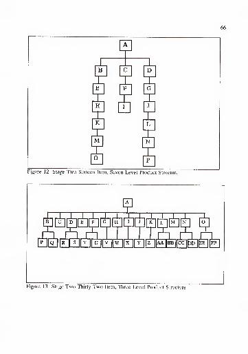
66

Figure 12 Stage Two Sixteen Item, Seven Level Product Structure

1B C D E F G ik; I J K L M N o

F r 7 rn Fi FP Q R

1S T U V

1

1>c 1 1 CC bD F.E FF

Figure 13 Stage Two Thirty Two Item, Three Level Product Structure

67

igure 15 Stage Two Thirty Two Items, Seven Levels Product Structure

68

Nine different demand patterns were employed in Stage Two, three generated from

a truncated normal distribution with a standard deviation of 75, three with a standard

deviation of 150, and three with a standard deviation of 300. In summary, three different

sizes and three different depths of product structure, four different cost sets and nine

different demand patterns were combined to yield 3*3*4*9 = 324 Stage Two

problems. In addition to obtaining solutions via seven different heuristics, lower bounds

on the optimal solutions were obtained for all Stage Two problems. This lower bounding

technique and its results are discussed in sections 4.4. 2.5 through 4.4.2.7.

3.2.5 Stage Two Computational Results

The results of the 8 item, 16 item, and 32 item problem .sets are displayed in

Tables 8, 9, and 10 respectively. Summary statistics for all 324 Stage Two problems are

displayed in Table 11. NlPPA(l) and NIPPA(2) ranked first and .second in relative co.st

performance acro.ss all three problem sets, both averaging within ]% of the optimal

solution. Graves’ algorithm, the only other multiple pass heuristic, consistently ranked

third, averaging only slightly more than 1% over the lower bounds on the optimal

solutions. Of the single pass heuristics, performances ranged from within 4% to within

14% of optimal. Here the rankings acro.ss the problem sets are not as consistent. For

example, STIL (featured in Stage One) ranked fifth in the 8 item and 16 item problem

sets, while it ranked fourth in the 32 item problem set.

69

Table 8 Stage Two Eight Item Product Structure Set, Computational Results Stated

Terms of Relative Cost with Respect to a Lr')wer Bound on the Optimal Solution

NIPPA(l) N1PPA(2) GRAVES CUMWW

STIL KCC SEQ WW

3 Levels:

n = 36

1.006 1.007 1.013 1.035 1.042 1.005 1.117

5 Levels:

n = 36

1.007 1.007 l.ai9 1.015 1.032 1.053 1.187

7 Levels:

n = 36

1.009 1.008 1.008 1.007 1.029 1.151 1.236

Standard

Deviation = 75

n = 36

1.007 1.009 1.014 1.018 1.050 1.081 1.192

Standard

Deviation = 150

n = 36

1.012 1.010 1.01

1

1.018 1.025 1.071 1.185

Standard

Deviation = 300

n = 36

1.003 1.003 1.005 1.02 1.029 1.057 1.161

Overall Average:

n = 108

1.007 1.007 1.010 1.019 1.034 1.070 1.180

Table 9 Stage Two Sixteen Item Product Structure Set, Computational Results StatedTerms of Relative Cost with Respect to a Lower Bound on the Optimal Solution

NlPPA(l) N1PPA(2) GRAVES KCC STIL CUMWW

SEO WW

3 Levels:

n = 36

1.007 1.007 1.011 1.005 1.044 1.060 1.065

5 Levels:

n = 36

1.012 1.013 1.011 1.007 1.046 1.060 1.118

7 Levels:

n = 36

1.010 1.011 1.017 1.046 1.032 1.035 1.180

Standard

Deviation = 75

n = 36

1.011 1.011 1.018 1.022 1.048 1.050 1.137

Standard

Deviation = 150

n = 36

1.013 1.013 1.017 1.020 1.036 1.052 1.125

Standard

Deviation = 3(K)

n = 36

1.006 1.006 l.ai3 1.016 1.038 1.053 1.101

Overall Average;

n = 108

1.009 1.010 1.012 1.019 1.041 1.049 1.122

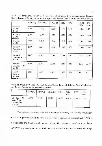
70

Table 10 Stage Two Thirty Two Item Product Structure Set, Computational ResultsStated Terms of Relative Cost with Respect to a Lx^wer Bound on the Optimal Solution

NlPPA(l) NIPPA(2) GRAVES STIL KCC CUMWW

SEQWW

3 Levels:

n = 36

1.010 1.011 1.009 1.045 1.010 1.081 1.05

5 Levels:

n = 36

1.008 1.009 1.016 1.036 1.028 1.052 1.113

7 Levels:

n = 36

1.007 1.008 1.014 1.028 1.111 1.032 1.196

Standard

Deviation = 75

n = 36

1.009 1.011 1.019 1.045 1.053 1.054 1.135

Standard

Deviation = 150

n = 36

1.012 1.012 1.017 1.033 1.051 1 .056 1.118

Standard

Deviation = 300

n = 36

1.004 1.004 1.004 1.031 1.045 1.055 1.107

Overall

Average:

n = 108

1.008 1.009 1.013 1.037 1.050 1.055 1.12

Table 11 Stage Two Computational Results, Stated Terms of Relative Cost with Respectto a Lower Bound on the Optimal Solution

NIPPA(l) NIPPA(2) GRAVES STIL CUMWW

KCC SEQWW

Average of All

Stage TwoExperiments:

n = 324

1.0093 1.0096 1.0128 1 .0373 1.0410 1.0463 1.1412

The variety of heuristics included in the Stage Two study provides the opportunity

to assess the performance of the various approaches to multiple stage planning, in addition

to comparing the average performances of specific heuristics. Analysis of variance

(ANOVA) was conducted on the results of each heuristic’s application to the 324 Stage

71

II, illlli,. u,., m ,« .« 0

, i«»iw 1^17 iW5i« 104,* ll»„.

Standard

Deviation of

Demand = 75

1 UOS 1X>1 [A\s U2 \02S ]j» 1^85 mStandard

Deviation of

Demand - 150

Standard

Deviation of

Demand - 300

Mgure 16 Histograms of the Stage Two Relative Cost Ratios of NIPPA(l), Groupedby the Experimental Factor of Standard Deviation of End Item Demand

Two experiments, to assess what impact, if any, the experimental factors may have had

on the relative cost performance of the heuristic. However, ANOVA requires the

assumption that the populations under study be normally distributed with the same

variances. Inspection of the relative cost ratio data did not support such an assumption.

Figure 16 displays one example, the three histograms of the relative cost ratios of

NIPPA(l), grouped according to the level of standard deviation of end item demand

present in the experiment.

While the required ANOVA assumption may seem appropriate for the first two

distributions, it is clearly violated by the apparent distribution of NlPPA(l)’s relative cost

72

30

0 01 0i> 0) 04 05 00 07 00 00 1

Standard

Deviation of

Demand = 75

Standard

Deviation of

Demand =150

Staiidard

Deviation of

Demand = 300

figure 17 Histograms of the Power Transformation of the Stage Two Relative CostRatios of NIPPA(l), Grouped by the Experimental Factor of Standard Deviation of EndItem Demand

ratios for experiments with the highest level of demand standard deviation. Initially,

transformation of the relative cost data was attempted, as was done in the heuristic study

of Sum, Png, and Yang [87]. First, the natural log of each ratio was calculated, but the

distributions exhibited by these numbers appeared only slightly less appropriate than those

of the raw data. Next, a Box and Cox [23] power transformation was estimated for each

heuristic (as discussed in Kuehl [61]), and new data sets were generated by raising the

raw data sets to their appropriate power. In the case of NIPPA(l), each relative cost ratio

was raised to the power of -84.6, and hi.stograms of the resulting data are displayed in

73

Figure 17. When Figure 17 is compared to Figure 16, the power transformation does

appear to have mitigated the problem of unequal variances between factor levels, but the

histogram of the third level remains drastically skewed. For this rea.son, transformation

of the relative cost ratio data was abandoned, and the rank of each relative cost ratio

within each heuristic’s Stage Two problem set was calculated. Unlike the ratios

themselves, the rankings of the ratios reasonably meet the required ANOVA assumptions.

(Figure 18 shows the ratio ranking histograms for the same example addressed by Figures

16 and 17.) Therefore, the ANOVA tests of Stage Two were conducted on the ranks of

the relative cost ratios within each heuristic’s set of results.

Standard

Deviation of

Demand = 75

Standard StandardDeviation of Deviation of

Demand - 150 Demand = 300

-igure 18 Histograms of the Ranks of the Relative Cost Ratios of NlPPA(l), Groupedby the Experimental Factor of Standard Deviation of End Item Demand

74

Tables 12 and 13 display the ANOVA results. The relationship between demand

variability and the average rank of relative cost ratios performance of a heuristic was

statistically significant for six of the seven heuristics, an observation consistent with past

studies (Roundy [78], Sum, Png, and Yang [87]). An interesting distinction between the

single pass and multiple pa.ss algorithms is their apparent degree of sensitivity to the

number of levels within the product structure. This factor is statistically significant for

all single pa.ss algorithms, while it is not significant for the three multiple pass algorithms.

The interaction of the size of the product structure and the number of levels was typically

the only statistically significant interaction factor for any heuristic, with the exception of

Graves’ algorithm (multiple interaction factors were significant), STIL and CUM WW (no

interaction factors were significant).

Average CPU time for each heuristic over each problem set is displayed in Table

14. These running times are stated in seconds, on an EVEREX 486/33 personal computer

with math coprocessor.

75

Table 12 ANOVA Tests of Multiple Pass Heuristic Response to Stage Two ExperimentalFactors

Heuristic

Source’ DF F Value Prob > F

NIPPA(l)

SD 2 77.11 0.000

ITEMS 2 3.50 0.032

LEVELS 2 0.27 0.761

SDHTEMS 4 0.18 0.946

SD*LEVELS 4 0.79 0.534

ITEMS*LEVELS 4 3.62 0.007

SD*ITEMS*LEVELS 8 0.28 0.971

N1PPA(2)

SD 2 80.74 0.000

ITEMS 2 5.60 0.004

LEVELS 2 0.28 0.758

SD*ITEMS 4 0.08 0.987

SD*LEVELS 4 0.70 0.592



GRAVES

SD 2 130.23 0.000

ITEMS 2 5.87 0.003

LEVELS 2 0.82 0.442

SD*ITEMS 4 5.36 0.000

SD*LEVELS 4 2.22 0.067


SD*ITEMS*LEVELSW" 1

8 0.62 0.764

^ Ihe experimental factors are SU = standard deviation of end item demand, ITEMS =the number of items in the product structure, and LEVELS = the number of levels in the

product structure.

76

Table 13 ANOVA Tests of Single Pass Heuristic Response to Stage Two ExperimentalFactors

Heuristic

Source* DF F Value Prob > F

KCC

SD 2 3.01 0.021

PTEMS 2 04.26 0.000

LEVELS 2 553.37 0.000

SDMTEMS 4 0.30 0.881

SD'LEVELS 4 0.63 0.644

ITEMS'LEVELS 4 21.37 0.000

SDMTEMS* LEVELS 8 0.53 0.836

STIL

SD 2 4.52 0.012

ITEMS 2 17..34 0.000

LEVELS 2 0.75 0.000

SD*ITEMS 4 0.81 0.5 19

SD*LEVELS 4 1.13 0.344

ITEMS'LEVELS 4 0.10 0.942

SD'ITEMS* LEVELS 8 0.23 0.948

CUM WW

SD 2 0.10 0.906

ITEMS 2 103.17 0.000

LEVEl^ 2 -34.24 0.000

SD*ITEMS 4 0.06 0.994

SD*LEVELS 4 0.05 0.995



SEO WW

SD 2 .30.20 0.000

ITEMS 2 16.3.13 0.000

LEVEI.S 2 654.76 0.000

SD'ITEMS 4 U7 0.325

SD'LEVELS 4 1.00 0.362

ITEMS‘LEVELS 4 1.3.26 0.000

SD*ITEMS*LEVELS—::—i i l- x

8 0.25 0.981

* Ihe experimental factors are SU = standard deviation of end item demand, ITEMS =

the number of items in the product structure, and LEVELS = the number of levels in the

product structure.

77

Table 14 Average CPU Times of Stage Two Experiments*

Eight Item Product

Structures

Sixteen Item

Product Structures

Thirty Two Item

Product Structures

KCC 0.025 seconds 0.045 seconds 0.100 seconds

CUM WW 0.039 0.047 0.055

STIL 0.043 0.090 0.212

SEQ WW 0.117 0.1536 0.361

GRAVES 0.271 0.580 1.514

NIPPA(2) 0.307 1.188 4.372

NIPPA(l)^ 1 ^

0.433 1.302 4.263

CPU time on an EVEREX 486/33 personal computer with math co-processor.

3.2.6 Alternate Stage Two Eight Item Cost Set

Inspection of Table 1 1 suggests that the relative cost performances of the STIL

and CUM WW algorithms are comparable, when applied to the Stage Two problem sets.

While CUM WW was not included in Stage One, it was included in Coleman and

McKnew’s study [26] after which the experimental design of Stage One was modeled.

A review of the re.sults of the original study yielded an interesting contradiction: STIL

was reported to have vastly outperformed CUM WW in these experiments. Although

bounds on the optimal solutions were never found for Coleman and McKnew’s "Phase

Two" experimenfs, STIL clearly outperformed all other heuristics (all SP-SLA's) in their

study. In particular, the relative co.st of applying CUM WW versus STIL was an average

of 1.109 over the 524 Phase Two problems, representing a nearly 11% cost penalty

incurred by the use of CUM WW versus STIL. The 8 item, 36 period problem set of

Stage Two provides the closest "match" to these 9 item, 52 period problems in terms of

78

size of the experiments, yet the average performance of STIL versus CUM WW remains

reversed, with a 1.5% cost penalty incurred by STIL versus CUM WW. In addition, SEQ

WW, on average, performed better than CUM WW in the Coleman and McKnew study.

In Stage Two of this investigation, SEQ WW consistently ranked last in terms of relative

cost.

This raises the question of how can the relative performances of heuristics vary

so widely across different studies? To explore this, another 8 item problem set was

appended to the Stage Two investigation. This problem set was identical to the original

8 item set across all but one factor: holding and ordering costs. In this problem set, item

costs were determined in the manner described in section 3.2.2, utilizing ordering cost

factors of 0.4 and 0.8, and holding cost factors of 1.1 and 2.0 to generate the four cost

sets. Table 15 displays the results.

Table 15 Stage Two Special Cost Eight Product Structures, Computational Results StatedTerms of Relative Cost with Respect to a Lower Bound on the Optimal Solution

NIPPA(l) NIPPA(2) GRAVES KCC STIL SEQWW

CUMWW

3 Levels: (n = 36) 1.007 1.008 1.011 1.014 1.020 1.106 1.067

5 Levels: (n = 36) 1.006 1.007 1.005 1.015 1.016 1.112 1.273

7 Levels: (n = 36) 1.004 1.005 1 .006 1.018 1.017 1.145 1.295

Standard Deviation =

75: (n = 36)

1.008 1.009 1.009 1.018 1 .025 1.131 1.246


150: (n = 36)

1.008 1.009 1 .009 1.016 1.014 1.123 1.212


300: (n = 36)

1.001 1.001 1.005 1.013 1.014 1.109 1.177

Overall Average:

(n = 108)

1.006 1.007 1.008 1.016 1.018 1.121 1.193

79

Despite the alternate cost set, the overall performance and rankings of the three

multiple pass heuristics remains virtually unchanged. Within the single pass heuristics

however, the results displayed in Table 15 vary from the corresponding results in Table

8. Now the rankings of STIL, SEQ WW, and CUM WW coincide with the results of

Phase Two of the Coleman and McKnew study. In addition, the relative cost performance

ratios of the sequentially based single pass heuristics appear to have improved with the

exchange of cost sets. Comparison of Tables 8 and 15 show that KCC’s average relative

cost ratio declined from 1.070 to 1.016, STlL’s average relative cost ratio declined from

1.034 to 1.018, and SEQ WW’s declined from 1.179 to 1.121.

3.3 Concluding Remarks

The scope of the Stage Two experiments, in terms of the variety of "improved"

heuristics evaluated, is of a degree previously unavailable in the multiple stage planning

literature. The computational results of both Stage One and Stage Two provides evidence

of NIPPA s effectiveness as a new multiple stage planning heuristic. Graves' algorithm

also performed well, but the difference between the performances of the.se two algorithms

is significant. If the Stage Two relative cost ratios of either NIPPA(l) or NIPPA(2) are

combined with the relative cost ratios of Graves algorithm and ranked, the difference of

between the average rankings is statLstically significant in either ca.se, with a p-value near

0.000. In contrast, combining and ranking the relative cost ratios of NlPPA(l) and

NIPPA(2) to perform the same hypothesis test yields a p-value of 0.301, indicating that

there is not a statistically significant difference between the average performance of these

two heuristics, relative to each other. Thu.s, the starting .solution .scheme of NIPPA(l),

80

described in section 3. 1.3. 4, is of doubtful merit. The intention of alternate starting

solutions for the NIPPA search was to identify solutions that both terminate in "high

quality" final solutions and save on computational time. In addition to failing to

distinguish itself in terms of final solutions, the Stage Two starting solution scheme

actually increased average computational time for the 8 and 16 item problem sets. As a

result ofthe.se observations, the initial .solution used in a NIPPA .search will be lot-for-lot,

from this point forward in the investigation.

The broader scope of the Stage Two investigation provides an opportunity to make

comparisons in heuristic performance, with respect to the taxonomy discu.ssetl in Chapter

2. The computational efficiency of single pa.ss algorithms is highlighted by the data in

Table 14, yet the general inferiority of their solutions, relative to multiple pass technique.s,

is suggested by the relative cost rankings of every problem set. In addition, the Stage

Two results suggest another weakness that this class of heuristics appears to share;

sensitivity to problem size. Although the computational burden of applying the multiple

pass heuristics to the Stage Two experiments grew quickly with the number of items, the

relative cost performance of these heuri.stics only declined slightly. This was not the ca.se

with any of the five single pa.ss heuristics tested. An increa.se in the number of items

within the product structure resulted in either an erratic shift or a distinct decline in

relative cost performance of the single path heuristics. These heuri.stics also displayed

a marked sensitivity to the number of levels in the product structure, which did not test

statistically significant for any of the multiple pass heuristics. It is interesting to note that

the relative cost performance of CUM WW appears to improve with the number of levels

81

in a product structure (from an overall average of 1.0591 for 3 level structures to an

overall average of 1.0259 for 7 level structures), while the relative cost performance of

single pass, sequential heuristics tends to deteriorate (SEQ WW slid from an average of

1.0777 for 3 levels to 1.2051 for 7 levels). CUM WW was al.so the only heuristic for

whom the standard deviation of end item demand and the item*levels inteniction term

were not statistically significant factors in the ANOVA of its Stage Two ranked relative

cost ratios.

Repeating the eight item Stage Two experiments with an alternate cost set

generated in the style of .some earlier heuristic studies revealed an interesting i.ssue in

multiple stage experiment design. The relative performance of single pass heuristics, as

well as the quality of their respective .solutions, can vary widely with the researcher’s

choice of experiment cost structure. Generating holding and ordering costs hy .selecting

a value to the lowest (childless) items and applying some multiplictitive factor to

determine costs at higher levels (for example, Coleman and McKnew [26], Veral and

Laforge [90]) appears to "favor" the .sequentially applied single pa.ss heuristic. While

their performance did not surpa.ss that of the multiple pass heuristias, it did improve

considerably with respect to the optimal .solution, and the performance rankings of the

single pass heuristics changed dramatically with the change of cost sets used in the eight

item Stage Two problems. This effect may be related to the character t>f cost sets

generated in the "multiplicative" style, for the majority of the schedule’s total costs is

concentrated in the lowest levels of the product structure. Generally (dependent on the

actual cost factors u.sed), the magnitude of the combined ordering and holding co.sts

82

declines as one moves up the product structure, where it may be near trivial for the end

item. (For example, the ordering cost of a childless item was fixed at $50. Using the

order cost factor of 0.4, the ordering cost for the end item of a seven level structure is

$0.2048.) Originally, the cost aspect of the Stage Two experiment design was changed

to randomly chosen item costs (such as Afentakis and Gavish [1], or Blackburn and

Millen [20]) to avoid the wide variation in AOC observed in the Stage One experiments.

However, this shift in experiment design has revealed an important les.son in multiple

stage planning heuristic evaluation: it may be unwise to draw conclusions concerning the

relative merits of various single pass heuristics without careful attention to the nature of

the holding and ordering cost sets employed in the evaluation.

CHAPTER 4

MATHEMATICAL PROGRAMMING FORMULATIONS AND BOUNDINGPROCEDURES FOR MULTIPLE STAGE PLANNING PROBLEMS WITHOUT

JOINT COSTS OR CAPACITY CONSTRAINTS

4.1 Introduction

As discussed in Chapter 2, the computational costs of obtaining an optimal

solution to a multiple stage planning problem of even modest size is generally prohibitive

for most researchers and practitioners alike. While this has fueled the development of

heuristics, it has also hampered the evaluation of their relative merits. Too often,

investigations state the observed performance of a heuristic relative to other heuristics

(see, for example. Sum, Png, and Yang [87], Bookbinder and Koch [22], or Veral and

Laforge [90]). If it is impractical to obtain optimal solutions for use as benchmarks, then

lowerbounds on these .solutions can be obtained for the same purpo.se. The lower bounds

used in Chapter 3 were obtained through the techniques developed in this chapter.

To gain insight into the optimal .solution of a multiple stage planning problem, we

begin by examining mathematical formulations of that problem. Section 4.2 pre.sents two

such formulations from the literature, and introduces a new one. Section 4.3 proposes a

method of reducing the size of these formulations, to ease the computational burden

implied by their use. The lower bounding technique explored in this chapter employs

Lagrangian relaxation, and is discussed in section 4.4. Consistent with the experiments

83

84

of Chapter 3, we will assume that holding and ordering costs are positive throughout this

chapter.

4.2 Problem Formulation

4.2.1 The Mixed Integer Formulation

The following mixed integer formulation of the multiple stage planning sizing

problem without joint costs or capacity constraints is e.ssentially that of McClain et al.

[72]. This mixed integer approach is typical of much of the earlier mathematical

programming developed for multiple stage planning, including Steinberg and Napier [84],

Afentakis, Gavish, and Karmarkar [2], Crowston and Wagner [29], and Zangwill

[95][96].

J TMinimize Y. E ( r,.P,. + /«./.. + )

i=l

Subject to:

I«-i. j

- -'u - K

P, - my, < 0

Yij = {0,1}; Pij, lij > 0 for allJ= 1, ..., J; i = 1, ..., T

Where:

J,_ . 1 if at least one of item j is ordered in period i

V 0 otherwise

J = the total number of items

T = the total number of planning periods

85

Pij = the quantity of itemj ordered in period i

= the inventory of item j at the end of period i

j= the parent of item

j

= the cost of producing an itemj

in period i

hjj = the cost of holding an itemj in inventory during period i

S;- = the ordering cost of itemj

in period i

bjj = external demand for itemj

in period i

a-. = the number of child itemsj needed to produce a parent item j*

M = a number larger than the maximum of for all i,j

The only variables with integer requirements are the Yjj’s, representing whether

at least one of some item was ordered in some period. The values of the two other

decision variables, the P^j’s and Ijj’s, are not restrained to zero or one, for they represent

the actual amount of an itemjordered in a certain period i and existing in inventory at

the end of period i, respectively. The first set of constraints relates the action to ordering

in a multiple stage environment to the resulting levels of inventory. These constraints

dictate that the amount of a particular item i in inventory at the end of the prior period

plus the amount ordered in the current period, less the amount consumed by an order for

that item’s parent, must equal the amount left in inventory at the end of that period plus

the amount required by external demand for that item in that period (if any). The

remaining set of constraints simply "triggers" = 1 if P;. > 0.

If production costs do not vary over time, the objective function can be simplified

to reflect minimization of the holding and ordering costs only:

J TMinimize J] ^ + 5 .I;. )

j=\ i=l

Variation in production cost can be incorporated into any of the formulations and

techniques discussed in this chapter, as well as many of the heuristics studied in Chapter

3 (including NIPPA). For simplicity’s sake, however, production costs will be assumed

constant throughout this investigation. Another assumption of this formulation is that the

leadtimes on the production of all items are zero. As discussed in Chapter 1, there is no

loss of generalization due to this assumption, provided that actual leadtimes are constant

and independent of order size. To simplify notation and reduce computations, the

assumption of zero leadtimes has been made for all formulations and experiments in this

investigation.

4.2.2 The MSC Pure Binary Formulation

Recently, a different approach to the formulation of multiple stage planning

problems was presented by McKnew, Saydam, and Coleman [73]. This approach has

been dubbed a "pure binary" formulation in this investigation, ba.sed on one of its

intriguing features: unlike earlier formulations, this mathematical program is constructed

entirely of binary, or "zero-one" variables. What follows is such a formulation, for a

problem involving no joint costs and constant production costs:

J T T k-\

Minimize E E * E EE Wm7=1 1=1 j€{Z) k=2 i=l

T k-l

" E E EMZ] k=2 i=l

Subject to:

87

V- i-ljji- Y.. <

V- 0

0

Xij,= {0,l}; Yij = {0,l}

Where:

j= 1, J

k = 1, ..., Ti = 2, k

Allj in {Z}

k= 1, Ti = 1, k-1

if demand lot k of item j has been ordered in or prior to period i

otherwise

y _ 1 1 f least one of item j has been ordered in period i

V 0 otherwise

{Z} = the set of all items which possess a parent item.

djj = the "demand lot" of itemj

in period i, the amount of itemjneeded to supply the

external or dependent demand requirements of itemj in period i.

When comparing the formulation in Section 4.2.1 to this formulation, a

clarification should be made. Here the parameter d,j is called the "demand lot i" of item

j, and the need for clarification stems from the use of the word "lot". Traditionally, the

term lot refers to an order for an item, the size of which is determined by the decision

maker. One conventional lot scheduled for a certain period may be the sum of several

demand lots of an item. Demand lots are, as discussed in Chapter 1, fixed external

parameters. If an item is an "end item", its demand lots are the external demand for that

item (djj = b^j, for i = 1, ..., T). If the item is a non-end item, its demand lots are the

amounts of that item necessary to supply the external demand requirements of the end-

item (d|j = a-.d-., where j’ is the parent of item j).

88

In this formulation, the definition of the Y- binary ordering variables remains

unchanged from the mixed integer formulation. However, the expression of order size

(Pij from the mixed integer formulation) is quite different. Here, ordering decisions are

modeled in terms of whether a particular demand lot of a particular item has been ordered

in or before a particular period. Thus, the first set of constraints could be thought of as

the "horizontal" constraints, in that they enforce the condition that, if a demand lot has

been ordered on or prior to a period (some = 1), it must have been ordered prior to

the next period = 1). The second set of constraints "triggers" an item’s ordering

variable, just like the second set of constraints in the mixed integer formulation. Due to

the revised definition of the decision variables, however, the logic expressed is somewhat

different: if a demand lot is ordered on or prior to a period (some X|j,^ = 1), it must have

been ordered on or prior to the previous period (X|.,j|^= I)> it must have been ordered

in that period (Yy = 1). The third set of constraints enforce the parent/child relationships

necessary to the product structure, by requiring an item’s demand lot to have been ordered

on or prior to some period (Xy,j = 1) if its parent’s corresponding demand lot has been

ordered on or prior to that period (Xy.^, = 1).

One important feature of the MSC pure binary formulation is its implicit

incorporation of the "Wagner-Whitin" properties into any feasible solutions. Originating

in [92], extended to uncapacitated multiple stage problems by [89] (among others), and

discussed again in Proposition 2 of .section 4.3.1 of this chapter, there exists an optimal

solution that, for any period in which an order is placed for an item, the previous period

posse.sses zero ending inventory (the Wagner-Whitin property). Thus, production of a

89

demand lot cannot be "split" over more than one period in a solution satisfying these

conditions. Expressing inventory as whether or not an entire demand lot is present

= 0 or 1) partially enforces Wagner-Whitin properties on all solutions feasible to this

formulation.

Another important note concerning this model is that backlogging is not

permitted. Therefore, the variables k = 1,...,T, are not variables at all, but constants:

= 1, for k = 1,...,T.

4.2.3 The Modified MSC Pure Binary Formulation

For the purpose of this investigation, we will rely on a slight modification of the

original McKnew, Saydam and Coleman pure binary formulation. The only feature of

this formulation that differs from that of the preceding section is the objective function.

For the modified formulation, we propose the objective function:

J T J T k-l

Minimize E E Ve * E E;=1 i=l 7=1 k=2 i=l

Where:

Cjj = the incremental, or "value added" cost of holding an itemj

in inventory during

period i.

The distinction between the two formulations is the use of holding costs (hjj),

versus incremental holding costs (c-). Incremental holding costs (used in the

computations of NIPPA) are also known as "value-added" or "echelon" holding costs, and

they relate to the holding costs in .sections 4.1.1 and 4.1.2 in the following way:

= h - E h age{Gj}

^ ^

Where:

{Gj}= the .set of all children of item j.

90

= the number of item g required to assemble one item j.

To see the relationship between the two formulations, consider restating the

objective function of section 4.2.2 as:

Minimize E ^ij ^ E E E;=1 i=l j=l k=2 1=1

T k-l

- ^ E E W-..,ye{Z} k=2 i=l

Recall that ajj. is the number of itemsj

needed to build the parent item j’

Therefore d;j = ajj.d^j., for any item in {Z}. Using this, we can state:

J T J T k-l

Minimize Y, E * E E E WiH;=1 1=1 ;=1 k=2 1=1

T k-l

E E Eit=2 1=1

Let {Gj} be the set of all children of itemJ.

We can restate the expression above as:

J T J T k-l

Minimize E E + E E E <

;=1 1=1 7=1 ^=2 i=l

Restated:

J T J T k-l

Minimize E E " E E E V''(/ ‘ ,“A)7=1 i = l 7=1 )t=2 1 = 1

ijk

91

In addition to providing an alternate approach to the mathematical programming

of a multiple stage planning problem, the pure binary formulation possesses several useful

attributes not found in the older mixed integer approach. These attributes will be

discussed in detail, later in this chapter.

4.2.4 A New Pure Binary Formulation

One of the major di.sadvantages of the pure binary approach to modeling a multiple

stage planning problem is the size of the resulting formulation. Consider a problem

which consists of J items within the product structure, and T planning periods. What

follows is the size of corresponding mathematical program, given the mixed integer versus

pure binary approach:

MIXED INTEGER FORMULATION:3*J*T decision variables

2*J*T constraints

PURE BINARY FORMULATION:T

+ J*T decision variables

z=l

T3*J*^i constraints

1=1

For example, a problem selected from among the eight item Stage Two

experiments would require 864 variables and 576 constraints, if formulated as a mixed

integer program. In contrast, the same problem would require 5,616 decision variables

and 15,984 constraints, if formulated as a pure binary program. Thus, a portion of this

investigation focused on developing new methods which might reduce the size of pure

92

binary multiple stage planning formulations. One result of this effort was the

development of an alternate pure binary formulation, requiring considerably fewer

constraints:

J T J T k-l k-1

Minimize Y. E * E E EE;=1 i=l ;=1 k=2 i=l g=i

Subject to:

k

i=l

j= 1, .... J

k = 1, T

1',. ^ 0

j= 1.

Tk

" Alljin{Z}

i = 1, T

{0,1}; {0,1}

Where:

^ _ I

1 i/ demand lot k of item j is ordered in period i

V* 0 otherwise

y _ 1 1 if tit least one of item j has been ordered in period i

V '0 otherwise

93

One of the principle differences between the new formulation and the modified

MSC formulation is the definition of the inventory variables X|j|^. Here these variables

only assume a value of one if demand lot k of itemj

is ordered in period i, dropping the

"in or prior to" logic of the older formulation. The Lssue of how long a demand lot has

been held in inventory is transferred completely to the objective function. Should the

incremental holding cost for all items be the same acro.ss all planning periods, the

statement of the objective function can be simplified to:

J T J T k-l

Minimize £ + E E E7=1 1=1 7=1 k=2 i=\

where Cj is the incremental holding cost of item j.

Modifying the definition of the inventory variables allows the requirement of

delivery of each demand lot of each item to be stated in a single constraint: the sum of

all inventory variables referring to a particular demand lot of a particular item must equal

one. The .second set of constraints are equivalent to the .second set of constraints of the

MSC formulation, requiring that the ordering variable Y - = 1 if any demand lot k of item

jis ordered in period i = 1).

The third set of constraints enforces the parent/child relationships of the product

structure, just like the third set of constraints in the MSC formulation, but in a different

manner. In the MSC formulations, these relationships were enforced through the

inventory variables, requiring one constraint for each such variable. In the new

formulation these relationships are enforced by placing constraints on the (le.ss numerous)

ordering variables, incorporating another well known feature of the optimal .solution to

94

such problems. This principle (see Crowston and Wagner [29]), restated in the notation

of this section, characterizes the set of optimal solutions to this problem as:

There exists an optimal solution with the property of Y-j = 1 implies 7^. = 1 for anyperiod i and any item j in fZ}.

This property is sometimes referred to as "nestedness" (for example, Roundy [78]),

and many heuristic algorithms employ it directly when producing a solution. This group

includes NIPPA, which will always provide a nested solution, provided that the starting

solution was nested. Requiring the all order schedules to be nested, however, does not

guarantee a feasible solution to the multiple stage problem. Indeed, there are solutions

feasible to the new pure binary formulation that are not feasible to the MSC formulation,

for they represent order schedules in which orders for parent items are not adequately

supplied by the order sizes of their children. While these solutions may be feasible to the

pure binary formulation, we can show that such solutions would never be optimal:

Proof. Suppose there exists an optimal solution S to the pure binary formulation

that violates the parent/child requirements of the MSC formulation. Thus, there exists at

least one demand lot k of .some itemjfor which some Xjj,, = 1 and = 1, where p <

i <= k and d|^j, > 0. Since the optimal solution to this formulation must be a feasible

solution, we know Y|j = 1 and Y-. = 1. Let S* be the feasible solution to this problem

which is identical to the solution S, with the exception of X;j.,^ = 1 and Xp^.^ = 0. The

minimum .savings of this revision results from the p-i periods of incremental holding cost

charges not incurred by demand lot k of item j*. The maximum cost of the revision is

zero (recall that Yij = 1 in both solution S and S ). Thus, due to the a.ssumption of

positive holding and ordering costs, the total cost of S* is less than the total cost of

95

solution S. S cannot be an optimal solution. Therefore, there cannot exist an optimal

solution to this problem which is infeasible with respect to some parent/child requirement

of the multiple stage planning problem.

Redefining the inventory variables and employing the above proof combine to

provide a pure binary mathematical program with the following requirements;

NEW PURE BINARY FORMULATION:T

+ J*T decision variables

i=l

TJ*^i + 2*J*T constraints

i=l

Recall that an eight item problem from Stage Two of the previous chapter would

require 5,616 decision variables and 15,984 constraints if modeled as an MSC pure binary

formulation. While the new formulation still requires 5,616 variables to model the same

problem, such a formulation results in only 5,904 constraints, representing a 63%

reduction over the MSC formulation.

4.3 Characteristics of the Optimal Solution

4.3.1 Earliest Economic Order Periods

While the new pure binary formulation is considerably smaller than the MSC

formulations in terms of constraints, it can still require a substantial number of variables.

In this section, we will develop a method of reducing, or "pruning", the number of

variables and constraints required by either formulation, based on the cost and demand

parameters of a given problem. If a multiple stage planning problem is free of capacity

96

constraints, it possesses an optimal solution or solutions with certain known

characteristics. In this section, these characteristics are combined to create the "Earliest

Economic Order Period" of any demand lot k of item j, or "EEOP^j". The EEOP of some

demand lot is the earliest period that a particular lot might be ordered in an optimal

solution. EEOP^j’s will be utilized in the following sections and chapters, both in the

application of heuristic procedures and in variable reduction logic for pure binary

formulations. Identification of the EEOP^j’s within a problem is derived from two

propositions:

Proposition One.

Consider a multiple level lot sizing problem in which the cost parameters Sjj and

C|j are non-negative, for all i and j. Let {Pj} be the set of all predecessors of any item j.

E ^ ) /

P^{Pj] P^\Pj]

for any item j.

Let M*i^ - [ J, where { x \ is the greatest integer ^ x.

M^j is the ratio of the total ordering costs required by the production of an item

(its ordering costs and that of all its necessary predecessors) to the total cost of holding

one particular demand lot of that item for one period. This ratio can be thought of as the

maximum number of periods that demand lot would be carried in inventory, if the item

had no parent with which to coordinate orders.

End item case. Let itemjbe an "end item", an item with no parent. In any

optimal solution, demand lot k of itemjwill be ordered no earlier than M\j periods prior

to period k.

97

Non-end item case. Let itemjbe a "non-end" item, an item possessing a parent

j*. In any optimal solution, demand lot k of itemjwill be ordered no earlier than

Qkj ~ ^ kj Qkj*

periods prior to period k. Should j* be an end item, 0|,j. = M\j.. Thus, Q^j, is defined

recursively, stemming from the calculation of M\j. of an end item.

Proof of End Item Case. Let S be a feasible solution to a multiple level lot sizing

problem without component commonality or capacity constraints. Suppose demand lot

k of end itemj

is ordered in period i in solution S, where k-i > Mi^j. Create solution S*,

identical to solution S, with the exception of the delivery of demand lot k of itemjand

all items in set {Pj}. In S*, let demand lot k of itemjand all items in {Pj} be ordered

in period k. Let TC and TC’ be the total costs associated with S and S*, respectively.

By scheduling the delivery of demand lot k ofjand {Pj} in period k, solution S* .saves

a minimum of k-i periods of holding cost for these items. Yet, by ordering in period k,

S* incurs a maximum of s,^j plus s,,p for all p in {Pj}, the ordering costs. Let dTC = TC -

TC*. Let dTC’ be the minimum possible value of dTC. Formerly,

dTC -

J

~ ~ ^'^p

J

^

If dTC’ > 0, the TC > TC*, regardless of the actual difference between TC and

TC*. Dividing dTC’ through by the minimum holding costs saved produces:

dTC/

^

^kp^kp )“ “ 0 “

By the statement of the problem, k-i > M,,j, thus (k-i) - M,,j > 0. Restated:

98

dTC' ! {d^c^ + E d^c^ ) > 0P^{Pj]

Since the minimum holding costs saved is a non-negative number, due to the fact

that d|(j and c^p are both non-negative parameters, multiplying the expression above

through by the denominator confirms dTC’ > 0. Thus, TC > TC*. So, for any solution

S in which any demand lot k of any end itemj is delivered in period i, where k-i > M|^j,

there exists a solution S with a lower total cost. S cannot be an optimal solution. Note

that M|jj £ M|jj, thus when k-i > holds, k-i > M

,(j

al.so holds, and S cannot be the

optimal solution.

Proof of the non-end item case. Proof of the non-end item case is an extension

of the end item case proof. Let S be a feasible solution, in which .some demand lot k of

some non-end itemj

is delivered in period i, where k-i > Q,^j. Let i* be the period in

which demand lot k of itemj

is delivered. If k-i > M^j., and j* is an end item, apply

"Proof of the End Item Case" to demand lot k of j* to show there exists S*, a solution

with lower total cost. If k-i > Q|^j,, redefinej as

j . Continue to redefinej until either

k-i* > M^j. and j* is an end item (apply "Proof of the End Item Case") or k-i* < 0,^^.. In

the event that k-i <.0|jj., create S , a solution identical to S with the exception of demand

lots k of itemjand all items p in set P^. These items are scheduled for delivery in i*, the

period in which demand lot k of parent itemj is delivered. We know the minimum

difference between TC and TC* is:

99

Dividing dTC’ through by the minimum holding costs saved produces:

dTC' ! + E - 0 -

Since M\j < M^j,

dTC /

As seen in the end item case, if we can show (i*-i) - M\j > 0, we can confirm

dTC’ > 0. Using the condition k-i > Q^j, we find i < k-Q^j. Likewise, k-i* < Q^., can be

restated as i > k-Q,^j.. Using these two expressions, we can state (i*-i) - M\j > ((k-Q,^j.) -

(k-Okj)) - M\j. Simplified,

Therefore, (i -i) - M > 0 and dTC’ > 0. TC* < TC, so solution S cannot be the

optimal solution to this problem.

Proposition Two.

Let D^j be the period in which demand lot k of some itemj is ordered. There

exists optimal solution, D,^j > MAX{ D,j, ...,

('*-') - - Q,j. - M\..

SubstitutingQ,^j = Q^j, + M\j into the expre.ssion,

(i*-i) - M\. > Q,.. + M\. - Q,.. - M\j.

100

Proof. One well known result from multiple level lot sizing literature is the

existence of an optimal solution in which Pijlj.g = 0 for each i andj in the mixed integer

formulation of section 4.2.1. (For proof, see Veinott [89]). Casually stated, there exists

an optimal solution in which, for any item j, an order in period i implies an ending

inventory of zero for the prior period. Suppose < D,^j, for some x<k of some item

j. This implies demand lot k of itemjwas in inventory at the end of period x-1, directly

prior to the order containing demand lot x.

From the first proposition, we proved that demand lot k of any item would be

ordered no earlier than period k - Q|,j. Now we combine the two propositions to construct

an iterative procedure to produce the Earliest Economic Order Periods for any demand

lot k of any itemj

(its "EEOP^j"):

a. Begin with end item j*’, and calculate EEOP^j.. = MAX (k -}for all k.

b. For k = 2, ..., T, if EEOP^... < EEOP,., ..., then EEOP,j.. = EEOP,., ... and Q,...

= MIN {Q,., ... + 1, k-1}.

c. Repeat EEOP,^j generation (steps a and b) for the children of j”.

d. Continue through the product structure in this fashion, until all EEOP^j have

been generated.

4.3.2 Variable Reduction Logic

As discussed in earlier sections, one of the primary di.sadvantages of the newer

pure binary mathematical formulations is their size. Now, employing knowledge of the

EEOPj^j’s, the size of a pure binary formulation may be reduced, the degree of reduction

being dependent on the cost and demand parameters. Variable reduction, or

101

"preprocessing" of the pure binary program, was first suggested by McKnew, Saydam and

Coleman [73]. However, they proposed dropping only end-item inventory variables based

on reasoning similar to the end item ca.se of Proposition One in .section 4.3.1. We

propose and will utilize a more aggressive preproce.ssing scheme, employing the Earliest

Economic Order Periods (EEOP’s) of all lots and all periods within a problem. As shown

in the proof in section 4.3.1, no demand lot will be ordered earlier than its EEOP in an

optimal solution. Specifically,

= 0 if i < EEOP|^j for any k, j.

Thus, these variables can be treated as con.stanLs, reducing both the number of variables

and the number of constraints. The formulation in section 4.2.3 can be restated:

J TMinimize ^

y=l i=lE

T k-\

E Ek=2 1=1

Subject to:

< 0

V'kX: 0

- ^ 0

Xij,= {0,l}; Yij={0,l}

j= 1, J

k = 1, ..., Ti = EEOP^j, ..., k-1

j= 1, J

k = 1, ..., Ti = EEOP|^j, ..., k

Allj

in {Z}

k = 1, ..., Ti = EEOP^j, ..., k-1

Likewise, the formulation of section 4.2.4 can be modified to:

102

J TMinimize

j=\ 1=1

J T k-\ k-l

E E E EW.)7=1 k=2 i=l g=i

Subject to:

k

Ei=EEOP.

hk = 1

>9

j= 1, J

k = 1, T

-Y..^Q

h - ^ 0

j= 1, ..., J

k = 1, ..., Ti = EEOPi^j, ..., k

Allj

in {Z}

i = 1, T

4.3.3 Selected Computational Results

Table 16 di.splay.s the results of preprocessing the MSC pure binary formulations

of 5 sample problems from the Stage One, Phase Two experiments of Chapter 3. The

benefits of this scheme are dramatic: the number of decision variables required was

reduced by 60% - 92%. The degree of reduction is clearly related to the Average Order

Cycle of the pure binary problem. This follows from the fact that we are "trimming"

inventory variables from the problem; the longer the expected order cycles, the more

inventory variables will be required. While the variable reduction scheme does reduce

103

some of these 9 item, 52 period problems down to a size acceptable to some LP

packages, obtaining the LP relaxation to modest size problems still appears unreasonably

burdensome. Even the example problems which allowed the most dramatic reductions

still included almost 1,000 decision variables and about 1,700 constraints. Therefore, the

next section explores an alternate method of pursuing bounds on the optimal .solution to

a multiple stage planning problem.

Table 16 Variable Reduction of Sample Stage One, Pha.se Two Problems

Problem Size

After

Preprocessing

Sample

Problem*

Average Order

Cycle

Number of

Decision

Variables

Number of

Constraints

%Reduction

of Variables

% Reduction

of

Constraints

M4: 1.6/0.4 4.29 981 1690 92% 95%

M3: 1.6/0.4 5.65 999 1742 92% 95%

S3: 1.6/0.4 9.29 2466 5861 80% 84%

S4: 1. 1/0.4 12.42 4212 11024 67% 70%

S4: 1. 1/0.8 14.69 5130 13557 60% 64%

^Sample problem refers to the first ot the nine Stage One, Phase I wo demand patterns,

with parameters described by the problem label. See Table 7 for problem label key.

4.4 Uwer Bounds on the Optimal Solutions

4.4.1 The LP Relaxation

The linear programming problem obtained by omitting the integer requirements

of an existing integer programming problem is called the "LP relaxation" of that problem.

The LP relaxation may be readily solved with the simplex method, where the

computational burden of .solving the original integer programming problem may prove

104

prohibitive. Should the optimal solution to the LP relaxation be all integer, it is also the

optimal solution to the integer program. If the optimal .solution to the LP relaxation

contains one or more non-integer variable values, the corresponding objective function

value can be used as a lower bound (in minimization problems) on the optimal objective

function value of the integer program.

When introducing the MSC pure binary formulation of multiple stage production

planning, McKnew, Saydam, and Coleman [73] claimed the LP relaxation of such a

formulation would always be integer. As discussed in Chapter 2, Rajagopalan [75]

showed this claim to be untrue. Integer optimal solutions are observed in practice,

indicating that the LP relaxation may, at least, provide a very tight relaxation of the pure

binary formulation ([75]). Likewise, only integer solutions have been observed in this

investigation, when solving the LP relaxations of selected Stage One, Pha.se Two

problems employing the new pure binary formulation. However, no proof is offered that

the LP relaxation of the new pure binary formulation will always be integer.

While the new pure binary formulation appears to pos.sess a similar "tightne.ss" of

LP relaxation observed in the original pure binary formulations, use of either formulation,

preprocessed or otherwise, can result in linear programs requiring hundreds, if not

thousands, of variables and constraints. This suggested an opportunity to develop an

alternate lower bounding scheme, one which could avoid the comjiutational effort usually

required by solving large linear programs. The alternate method, which was employed

to find bounds for Stage One, Phase One and Stage Two experiments of Chapter 3, is

described in the remainder of this chapter.

105

4.4.2 Lagrangian Relaxation

4.4.2.1 Introduction

FLsher [42] note.s that "one of the most computationally useful ideas of the 1970s

is the observation that many hard problems can be viewed as easy problems complicated

by a relatively small set of side constraints." Multiple stage production planning is

typical of such problems: if not for those constraints which enforce the parent/child

relationships, the optimal ordering schedule could be generated easily by applying a

shortest path algorithm to the demand requirements of each item within the problem.

Lagrangian relaxation offers an alternative to LP relaxation when finding bounds on the

optimal solutions to such problems, by dualizing the complicating constraints. For

example, consider the following integer programming problem:

Min cx

s.t. Ax < b

Dx < e

X > 0 and integral

If Ax < b were the "complicating" constraints of an otherwise easily solvable problem,

a useful Lagrangian relaxation could be created:

Min cx + u(Ax - b)

s.t. Dx < e

X > 0 and integral

u > 0

where "u" are referred to as the "Lagrangian multipliers" of this relaxation. In the case

of minimization, the optimal objective function value of the relaxation is a lower bound

on the optimal objective function value of the original problem.

106

In the case of multiple stage production planning, dualizing the parent/child

relationships reduces the multiple stage problem to several single item "subproblems,"

easily solved with a shortest path algorithm, such as the Wagner-Whitin [92], Afentakis,

Gavish, and Karmarkar [2] first proposed such a decomposition by relaxing the

parent/child relationships within a mixed integer formulation similar to section 4.2.1. To

find bounds on the optimal solutions to experiments in Chapter 3, this investigation

initially employed Ljigrangian relaxation of the modified MSC formulation (for bounds

on Stage One, Phase One), and then Lagrangian relaxation of the new pure binary

formulation (for bounds on Stage Two). The investigation of pure binary formulations

over the mixed integer formulation of Afentakis et al. [2] was motivated by three

attractive properties of the pure binary approach:

1. The LP relaxation of the integer program is often integer, as discussed in

section 4.4.1. Afentakis, Gavish and Karmarkar [2] provide a proof that the bounds found

by the Lagrangian relaxation of a mixed integer formulation of this problem (employing

subgradient optimization) will never be better than the bounds found by its LP relaxation.

Thus, in their work, this method is u.sed to pursue bounds on the optimal solution, and

a branch-and-bound methodology is adopted to identify optimal solutions. The frequency

of integer LP relaxation solutions to the pure binary formulation suggests that perhaps the

optimal solutions to such problem could be found directly with Lagrangian relaxation and

subgradient optimization (discu.s.sed later).

2. The pure binary formulation describes a smaller .solution space. Note that, due

to the nature of the decision variables, the only production schedules feasible to the pure

107

binary problem are those in which order sizes are the sum of some set of demand lots,

a feature of an optimal solution to the problem (an extension of the discussion in

Proposition Two of section 4.3.1.) Upon relaxation, the MSC pure binary formulation

provides the opportunity to discriminate between demand lots when creating penalties,

which may prove useful.

3. The pure binary formulation can be easily modified to further reduce the

solution space to only those solutions which satisfy the "earliest economic order period"

characteristics of the optimal solution, developed in section 4.3.1 and section 4.3.2. This

cannot be incorporated into the mixed integer formulation.

As discussed in section 4.4.1, one disadvantage of pure binary formulations is the

number of variables and the number of constraints required. Fortunately, this is not a

deterrent in the case of the Lagrangian relaxation, because the relaxation will be solved

as a set of shortest path problems. The following .sections will de.scribe a Lagrangian

relaxation technique employing the modified MSC pure binary formulation (section 4.2.3),

and the results of the bound finding efforts for Stage One, Phase One of Chapter 3.

Then, a similar technique employing the new pure binary formulation will be discussed,

accompanied by the bound finding results of Chapter 3’s Stage Two experiments.

4.4.2.2 Problem formulation for the modified MSC Pure Binary Formulation

Similar to Afentakis, Gavish, and Karmarkar [2], the pure binary formulation of

section 4.2.3 can be transformed into J single level lot sizing problems by dualizing those

constraints which enforce the product structure’s parent/child relationships;

108

Minimize

J

E7=1

T

Ei=l

T

Eit-i

E/e{Z} k=2 i=\

J

E7=1

r

Ek=2

U'k

k-l

Ei=l

ijk

Subject to:

j= 1, ..., J

k = 1, ..., Ti = EEOP|,j, ..., k-l

j= 1, J

k = 1, Ti = EEOPi^j, k

While the remaining constraints represent J independent subproblems, the costs

associated with these subproblems are not readily visible in the statement of the objective

function. Some algebraic revision of this formulation is necessary before the "effect" of

the Lagrangian multipliers becomes apparent. Let e represent the one item in this

multiple stage problem that does not possess a parent item (the end item). (In the case

of no component commonality, should there exist more than one end item, the problem

decomposes into independent subproblems, one for each end item). Now we can restate

the objective function as:

V - ^ 0

X., - X

Xij, = { 0,1 }; Y;. = { 0,1 }

109

J T T k-\

Minimize Y, E */(, * E E;=1 i=l k^2 i=l

T k-\

;e{Z} A:=2 i=l

Let {Gj} be the complete set of children of an item j. Now the objective function can be

restated as:

J T T k-1

Minimize Y E * E E ( * E )

j=l i=l k=2 i=l'

T k-1

ye{Z} k^2 1=1 g^{Gj

g^{G^]

Now the cost parameters associated with the J subproblems are more apparent.

The ordering cost of an item J, S|j, remains unaffected by the relaxation. However, the

"revised" cost of holding demand lot k of .some itemJ in inventory during some period

i is:

d.c..V V

- Ege{Gj}

if itemj is the end item (posse.ssing no parent), and:

E V-igk

g^{Gj)

otherwise. Thus, the per unit inventory charge of an itemj from demand lot k, held in

inventory during period i, can be stated as:

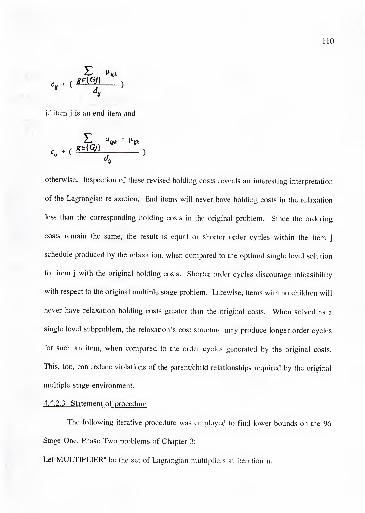
110

if itemj is an end item and

2̂ ^^t;Jt

. (*£1SL

,

otherwise. Inspection of these revised holding costs reveals an interesting interpretation

of the Lagrangian relaxation. End items will never have holding costs in the relaxation

less than the corresponding holding costs in the original problem. Since the ordering

costs remain the same, the result is equal or shorter order cycles within the itemj

schedule produced by the relaxation, when compared to the optimal single level solution

for itemj with the original holding costs. Shorter order cycles discourage infeasibility

with respect to the original multiple stage problem. Likewise, items with no children will

never have relaxation holding costs greater than the original costs. When solved as a

single level subproblem, the relaxation’s cost structure may produce longer order cycles

for such an item, when compared to the order cycles generated by the original costs.

This, too, can reduce violations of the parent/child relationships required by the original

multiple stage environment.

4.4.2.3 Statement of procedure

The following iterative procedure was employed to find lower bounds on the 96

Stage One, Phase Two problems of Chapter 3:

Let MULTIPLIER" be the set of Lagrangian multipliers at iteration n.

Ill

Let MULTIPLIER"(i,j,k) be the Lagrangian multiplier associated with relaxed constraint

^ij*k ^ijk < 0 at iteration n.

Let HOLD"(i,j,k) be the "revised" cost of holding one itemjfrom demand lot k in

inventory during period i, employed in iteration n.

Let MAX be the maximum number of iterations the procedure will execute.

Let n = 0.

Let TC"(j) be the total cost of the solution to the jth subproblem at iteration n.

JLet TOTALCOST" = TC"(f) at iteration n.

7=1

Let LOWERBOUND be the current lower bound on the optimal solution to the multiple

level problem.

Let SLACK"(i,j,k) = - Xj^, for k = 1,...,T; i = 1, ..., k-1; allj

in {Z}.

Let CONSTANT be a positive scaler, where 0 < CONSTANT < 2.

Let UPPERBOUND be the total cost of the NIPPA solution to the multiple level problem.


a. Let MULTI PLIER°(i,j,k) = 0 for all i,j,k.

b. Let HOLD"(i,j,k) = c- if i ^ EEOP|^j, and HOLD'’(i,j,k) = M, otherwi.se.

(Where M is a prohibitively large cost penalty.)

Step 1: If n > MAX, go to Step 7. Otherwise, go to Step 2.

Step 2: Solve subproblems.

a. Solve J single level lot sizing subproblems with a shortest path algorithm. The

single level demand requirements for any item g are the demand lots d^g (i=l,...,T). The

112

cost parameters of a single level problem of any item g are the ordering costs Sj^ (i = 1,

T) and the revised holding cost HOLD"(i,g,k) (k=l,...,T; i=l,...,k-l)

b. Calculate SLACK", based on the subproblem solutions.

Step 3: Update Lower Bound.

If n = 0, then LOWERBOUND = TOTALCOST”. Otherwise, if LOWERBOUND

< TOTALCOST", then LOWERBOUND = TOTALCOST".

Step 4: Check for violation of relaxed constraints.

If SLACK"(i,j,k) < 0 for all k=l,...,T; i=l,...,k-l; and allj

in {Z}, go to Step 5.

Otherwise, go to Step 6.

Step 5: Check for complimentary slackness.

If, for any SLACK"(i,j,k) = -1, MULTIPLIER"(i,j,k) = 0, then COMPSLACK =

YES. If COMPSLACK = YES, go to Step 7. Otherwise, go to Step 6.

Step 6: Update multipliers and holding costs.

a. Let MULTIPLIER"^’(i,j,k) = MULTIPLIER"(i,j,k) +

CONSTANT * (UPPERBOUND - TOTALCOST’')

\

J T t-1

E E E (SLACK’'{p^,t)f

g=l t=l p=\

* SLACK \ij\k)

for all k = 1, T; i=l, ..., k-1; allj

in {Z}.

b. Let HOLD"^‘(i,j,k) =

MULTIPLIER''*\ij\k) +

E MULTIPLIER’'^\ij,k)

113

for all k = 1,...,T; i = 1, k-1; allj

in {Z}.

Let HOLD""'(i,e,k) =

5T MULTIPLIER’'*\i,e,k)

for all k = 1,—,T; i = 1, k-1; and item e not in {Z} (the end item).

c. If TOTALCOST" < TOTALCOST" ' < TOTALCOST" ^ then CONSTANT =

CONSTANT / 1.1 .

d. Let n = n + 1. Go to Step 1.


If COMPSLACK = YES, LOWERBOUND i.s the total co.st of an optimal solution

to this problem. Otherwise, LOWERBOUND is a lower bound on the total cost of an

optimal solution. Stop.

The method used to determine the values of the Uigrangian multipliers at each

iteration is called subgradient optimization, first utilized in multiple stoge planning by

Afentakis, Gavish, and Karmarkar [2]. In subgradient optimization, the set of multipliers

at some iteration n+I is determined by

u""' = u" + t„(Ax" - b)

where;

1. t. = (q.(Z- - Z„(u-))) / IIAx- - b IP

2. 0 < q. < 2

114

3. Z* is an upperbound on the optimal solution.

4. Zp(u") is the objective function of the Lagrangian relaxation, employing the

set of multipliers from iteration n.

The value of the scaler CONSTANT in the description of the algorithm is set by

the user (provided that 0 < CONSTANT < 2 is true). An initial value of 2“’l0“’^, where

X= UPPERBOUND/TOTALCOST” was used in this investigation, with a 10% reduction

each time TOTALCOST" failed to improve over three iterations.

It should be noted that, for some arbitrary choice of values for the Lagrangian

multipliers, negative revised holding costs are possible. This would imply that a shortest

path algorithm, executed in Step 2, is inappropriate. However, by Proposition 5 of

Afentakis, Gavish, and Karmarkar [2], we can use a shortest path algorithm to solve the

L<igrangian relaxation subproblems, by treating the optimality condition discussed in

Proposition Two of section 4.3.1 as a set of redundant constraints of the original multiple

stage problem.

4.4.2.4 Computational results

The procedure described in .section 4.4.2.3 was coded in C and run on the 96

Pha.se One problems, with MAX = 50 iterations. Table 17 displays the results. Of the

96 problems, 83 converged on an optimal solution (a solution feasible to the original

problem satisfying complementary slackness, see Fisher [42] or Geoffrion [48]), nearly

80% of those requiring 5 or fewer iterations. On Table 17, this is referred to as the "First

Try." Of those that failed to converge to an optimal .solution, a "Second Try" was

devised, by repeating the procedure of section 4.4.2.3 with MAX = 100 and the initial

115

value of CONSTANT divided by 3. Ten optimal solutions were found, leaving only 3

of the 96 problems with lower bounds, but no optimal solution identified.

Table 17 Results of Stage One, Phase One Lower Bound Finding Efforts

Product

Structure

Number of

Optimal

Solutions

Found on

"First Try"

Number of

Optimal

Solutions

Found on

"Second Try"

Total

Number

of

Optimal

Solutions

Found

Number of

Optimal

Solutions

Found at First

Iteration

Structure #1

n = 24

24 n/a 24 10

Structure #2

n = 24

17 6 23 9

Structure #3

n = 24

22 0 22 11

Structure #4

n = 24

20 4 24 16

ColumnTotals

83 10 93 46

While these results are encouraging with respect to the usefulness of pure binary

Lagrangian relaxation, the figures in the extreme right column of Table 15 suggest

caution. Nearly 48% (46 of 96 problems) required only one iteration to identify an

optimal solution. This means that compiling the optimal solutions to the single item

subproblems resulted in a feasible, and thus an optimal, multiple stage schedule. Thus,

in nearly half of these experiments, Lagrangian relaxation with subgradient optimization

was not needed, and thus was not employed. This also casts doubts on the value of the

Stage One, Phase One experiments. If one views the parent/child relationships as the

116

"complicating" relationships of a multiple stage problem and thus the "source" of

difficulty when developing a multiple stage schedule, these experiments are arguably less

difficult. In nearly half of these experiments, the parent/child constraints were not

binding at the optimal solution, meaning they could have been ignored and optimal single

item techniques utilized to create an optimal multiple stage schedule.

4.4.2.5 Problem formulation for the new pure binary formulation

The new pure binary formulation, introduced in section 4.2.4, could be considered

preferable to the MSC pure binary formulation due to the fact that it requires fewer

constraints. However, for the purpose of Lagrangian relaxation, this can no longer be

considered advantageous, for both formulations decompo.se into J single item subproblems

of equal length. However, two features of the new pure binary formulation suggested that

it might still be preferable for the purposes of Lagrangian relaxation. The first feature

is simply the contrast in the number of parent/child requirement constraints that must be

relaxed. Employing the Lagrangian relaxation of a modified MSC formulation of some

Stage Two 8 item experiment may require relaxing as many as 5,328 constraints,

generating the need for up to 5,328 multipliers which must be updated at each iteration,

and incorporated into the revised costs of the relaxation. The Uigrangian relaxation of

the new pure binary formulation would require only 288 multipliers. The second

intriguing feature of the new pure binary Lagrangian relaxation is which costs are

modified by the choice of multipliers. Like the earlier work of Aftentakis, Gavish, and

Karmakar [2], the Lagrangian multipliers of the MSC formulation effect the holding costs

117

of the single item subproblems. However, Lagrangian relaxation of the new pure binary

formulation has a different effect on the subproblems:

Minimize

Subject to:

J T k-l k-l

E Ek=2

Ei=l

T

E EMZ] i=\

Eg=i

E Ei=\

k

Ei^EEOP,.

hk = 1

- y... ^ 0

j= 1, J

k = 1, Ti = EEOP|^j, k

p.. ^ 0

Xij,= {0,l}; Yj. = {0,1}

The effects of the multipliers on the costs of the subproblems can be highlighted

through algebraic manipulation of the objective function. Similar to the developments in

section 4.4.2.2, let e be the end item of this multiple stage problem. The objective

function can be restated:

118

J T k-\ k-\ TMimmKt E E E E * E

j=l k=2 /=1 g=i 1=1

T

J^{£\ i=l

Let {Gj} be the set of all children of an item j. Using this, the objective function

can be restated as:

J T k-\ k-\ TMinimize E E E E " E - E

y=l i=l f-i j=l «e|C.)

T

i^7\ ^1^ ~

pJtr 1JG{Z] 1=1 8^{Gj]

Further restated:

J T k-1 k-l TMinimize E E E E * E ‘ E

/=! t=2 i=l g^i i=l g6|G,|*

T

E E ~ E;e(Z| i=i ge\Gj] * '

At this point, the effects of the multipliers is clearer. Unlike the original

application of Lagrangian relaxation to multiple stage planning (Afentakis and Gavish [1],

Afentakis, Gavish, and Karmakar [2]) and the relaxed MSC formulation (section 4.4.2.2),

this relaxation revises the fixed ordering costs of the subproblems, not the inventory

holding costs. Note that the revised ordering cost for the end item will never be less than

its original ordering costs, implying equal or shorter order cycles in the subproblem

solutions. Likewise, this relaxation will never decrease the original ordering costs of

119

childless items, implying equal or longer order cycles for the subproblems that correspond

to the lowest levels of the product structure.

4.4. 2.6 Statement of procedure

At this point in the investigation, an iterative procedure was developed for bound

finding, employing subgradient optimization. The following statement of procedure is

similar to the procedure outlined in .section 4.4.2.S. Identical definitions have been

omitted.

Let MULTIPLIER"(i,j) be the Lagrangian multiplier associated with relaxed constraint Yjj.

• Y|j < 0 at iteration n.

Let ORDER"(i,j) be the "revised" cost of ordering at least one itemj

in period i,

employed in iteration n.

Let n = 0.

Let SLACK"(i,j) = Y... - Y,- for i = 1, ..., J; all j in {Z}.

Let HOLD(i,j) = qj if i > EEOP^j for all demand lots k held in inventory during period

i of a single item schedule, and HOLD(i,j) = M, otherwi.se. (Where M is a prohibitively

large cost penalty.)


a. Let MULTI PLIER”(i,j) = 0 for all i,j.

b. Let ORDER“(i,j) = S|j for all i,j.


Step 2: Solve subprohlems.

120


single level demand requirements for any item g are the demand lots dj^ (i=l,...,T). The

cost parameters of a single level problem of any item g are the revised ordering costs

ORDER"(i,g) and holding costs HOLD(i,g).


Step 3: Update Lower Bound.

If n = 0, then LOWERBOUND = TOTALCOST". Otherwise, if LOWERBOUND



If SLACK"(i,j) 0 for all i=l,...,T; and allj in {Z}, go to Step 5. Otherwise, go

to Step 6.

Step 5: Check for complimentary slackne.ss.

If, for any SLACK"(i,j) = -1, MULTIPLIER"(i,j) = 0, then COMPSLACK = YES.

If COMPSLACK = YES, go to Step 7. Otherwise, go to Step 6.


a. Let MULTlPLIER"^‘(i,j) = MULTlPLIER"(i,j) +

CONSTANT * (UPPERBOUND - TOTALCOST'^)* SLACK \ij)

E E iSLACK\t,g)?

\ 8^{Z) t=\

for all i=l, ..., T; allj in {Z}.

b. Let ORDER"^'(i,j) =

Sy + MULTIPLIER"*\ij) - ^ MULTIPLIER’'*\ij)g^{Gj]

121

for all i = 1, T; allj in {Z}.

Let ORDER""‘(i,e) =

Si^ + Z MULTIPLIER''*\i,e)8^{G^

for all i = 1, T; and item e not in {Z} (the end item).

c. If TOTALCOST" < TOTALCOST”' < TOTALCOST" % then CONSTANT =

CONSTANT / 1.1 .

d. Let n = n + 1. Go to Step 1.


If COMPSLACK = YES, LOWERBOUND is the total cost of an optimal solution



The value of CONSTANT used to obtain lower bounds on the Stage Two

problems differs from that used in section 4. 4. 2. 3. In this portion of the investigation, an

initial value of UPPERBOUND/(TOTALCOST"*X), where the value of X was initially

set at 12. If an optimal solution was not identified in 500 iterations, the entire process

was repeated with X = X - 2. The search for the lower bound on a particular problem

was limited to 4 such repetitions. Inspection of the output suggested that the repetition

process did not add much value to entire procedure: all but one optimal solution was

122

found with X = 12. For the problems for which an optimal solution was never identified,

the lower bounds produced from the varying initial values of X were not substantially

different.

4. 4.2.7 Computational results

Inspection of Tables 8 through 11 and Table 15 of Chapter 3 reveals that the lower

bounds found for the Stage Two experiments were within 1% of the optimal solution on

average, by virtue of the fact that they were, on average, within 1% of the best heurfstic’s

solution. Table 18 and 19 show the frequency of optimal solutions among those lower

bounds.

Table 18 Results of Stage Two Lower Bound Finding Efforts

Product

Structure

Number of

Optimal

Solutions

Found for 8

Item

Experiments

Number of

Optimal

Solutions

Found for

16 Item

Experiments

Number of

Optimal

Solutions

Found for

32 Item

Experiments

Total

Numberof

Optimal

Solutions

Eound

Numberof

Optimal

Solutions

Found at

First

Iteration

3 Level

Structure

23 24 23 70 0

5 Level

Structure

12 16 8 36 0

7 Level

Structure

13 13 11 37 0

Column

Totals

48 53 42 143 0

% of

Experiments

44.44% 49.07% 38.89% 44.14%

.

0%

123

Table 19 Results of Stage Two, Eight Item Special Cost Lower Bound Finding Efforts

Product Structure Number of Optimal

Solutions Found

Number of Optimal

Solutions Found at First

Iteration

3 Level Structure 29 8



Column Totals 83 22

Total as % of Experiments 76.85% 20.37%

It is difficult to draw any conclusions concerning the relative merits of the MSC

Lagrangian relaxation versus the new pure binary relaxation by comparing Table 17 to

Tables 18 and 19. Table 17 represents the frequency of optimal solutions found for five

item, twelve period problems. Tables 18 and 19 represent the frequency of optimal

solutions found for eight item, thirty six period problems. Despite the larger problems,

the new pure binary subgradient optimization technique still found optimal solutions to

44% of the 324 Stage Two Problems, and 77% of the 108 Eight Item, Special Cost set

problems of Chapter 3.

4.5 Concludinu Remarks

The lower bounds found for the Stage Two experiments of Chapter 3 represent

some of the most ambitious in multiple stage planning literature. Lagrangian relaxation

and subgradient optimization, when applied to the pure binary formulation, provided tight

bounds on the optimal solutions to experiments whose size had been previously

considered prohibitively large to undertake such an effort. Lagrangian relaxation of the

124

new pure binary formulation requires considerably fewer computations than the MSC

formulation, and the resulting revision of ordering (versus holding) costs is an approach

new to the body of Lagrangian multiple stage planning literature.

Tables 18 and 19, highlighting the number of optimal solutions of Stage Two

problems identified directly by the pure binary formulation relaxation, also underscores

observations made in Chapter 3. Choosing costs from a uniform distribution did not

produce any 8 item Stage Two problems which were solved at the first iteration of the

Lagrangian technique. Yet, simply switching to the "Special C(wt" set generated in the

manner prescribed by Coleman and McKnew [26] produced 22 of 108 problems (20%)

which were solved in one iteration. Despite the fact that each single item subproblem is

36 periods long, compiling these optimal single item .schedules into one multiple .stage

schedule resulted in no infeasible parent/child relationships in 22 ca.ses. This, coupled

with the fact that the proportion of optimal solutions found was substantially higher for

the special cost versus the uniform cost ca.se, again suggests that use of this multiple stage

cost structure creates experiments that are relatively easier to .solve.

CHAPTER 5

HEURISTIC PROCEDURES FOR MULTIPLE STAGE PRODUCTION PLANNINGPROBLEMS WITH JOINT COSTS DUE TO COMPONENT COMMONALITY

5.1 Introduction

As discussed in Chapter 1, the pre.sence of joint costs within a multiple stage

planning problem implies some item or items share one or more fixed ordering costs with

one or more other items within the product structure. Items sharing a joint ordering cost

belong to an item family. If one or more members of an item family are ordered in a

particular period, the item family ordering cost is incurred. If an item does not share its

ordering costs jointly with any other item, that item is the sole member of its family.

Component commonality is a specific form of the multiple stage joint cost

complication. Here, joint costs between items stem from the fact that these items are

actually identical components, incorporated into different branches of a product structure.

Thus, in the ca.se of component commonality, each item belongs to only one item family.

In addition, all items within a family must possess the same incremental holding costs,

for they represent multiple occurrences of the same component. While this problem only

models one form of joint costs in production planning, it is arguably the most popular

form discu.s.sed in the literature (for example, see Afentakis and Gavish[2], Bookbinder

and Koch [22], Graves [52], or Sum, Png, and Yang [87]). Most multiple stage planning

heuristics which can be applied to joint cost problems are restricted to ca.ses of component

125

126

commonality. This chapter will outline the computations necessary to apply NIPPA to

this popular form of the multiple stage joint cost problem, and evaluate it over two

experiment sets designed after the Stage Two problems of Chapter 3.

5.2 The Non-seguential Incremental Part Period Aleorithm (NIPPA)

5.2.1 Statement of the NIPPA Procedure with Component Commonality

Despite the introduction of component commonality, the decision rule employed

by NIPPA remains unchanged: eliminate the order which has the smallest ratio of

holding costs incurred to ordering costs avoided, provided that ratio is less than one.

However, orders now represent item families, implying that some ratios may repre.sent the

elimination of more than one item, provided the items belong to the same family. In the

case of any immediate predecessors, their orders are moved to the earliest feasible period

containing an order for their respective families. While the decision rule employed by

NIPPA is the same as that discussed in Chapter 3, the presence of component

commonality does modify the calculations necessary to employ this rule. To facilitate

these calculations, the following definitions should be amended to those of section 4.4.2.6:

Let f be the item family of some itemJand j‘* be the parent of that item.

Let z"(i,j) be the number of adjacent periods prior to period i, such that B"(i,g) = 0 for

all items g in {Ff}, given thatj

is an end item. IfJ

is not an end item, let z"(i,j) equal

+ the number of periods prior to period i - z"(i,j**)-l, such that B"(i,g) = 0 for all

items g in {Ff}. (This is an expanded definition of z"(i,j) from section 4.4.2.3.)

Let {FPf} be the set of necessary predece.s.sc^r families of item family f.

127

Let F"(i,f) be the number of items in {FJ for which orders are placed in period i, in

solution n.

Let X"(i,j) = 1 if B"(i,j) >0, and zero otherwise.

Let {FB"(i,f)} be the set of all items in {FJ for which an order is placed in period i in

solution n.

Let EFFECT\i/^) = - E E X\i,k)

Let NULLIFY"(i,f,g) = 1 if EFFECT"(i,f,g) = 0, and zero otherwise.

Ut COMMONJ^UMERATOR^ij) - E NUMERATOR\i^g^[Ff]

Ut COMMON_DENOMlNATOR\iJ) = E 5 *NULLIFY’'(i/,p)

P^{FP^]

Let COMMON_RATIOS"(i,j) = COMMON_NUMERATOR"(i,j) /

COMMON_DENOMINATOR"(i,j) if B"(i,j)>0, and zero othewise.


a. Generate B“, a feasible ordering schedule, such as a "lot-for-lot" solution.

Generate ORDER”, ZEROS”, and C0MM0N_RAT10S".

b. Find b(i‘, j’) = MIN {COMMON_RATIOS”(i,j)|

COMMON_RATIOS”(i,j) >

0 }.

Step 1:

If b(i, j ) ^ 1, go to Step 4. Otherwise, go to Step 2.

128

Step 2: Generate new solution and ratios.

a. Generate B".

i. Let B" = B"^'.

all items g in {Fj.}-

iii. B"(i’,g) = 0 for all items g in {Fj.}-

iv. For each item t in {Fj.}, let B"(i’-ZEROS" ‘(i*,tt), tt) = B" '(i*-ZEROS"

'(i ,tt), tt) + B""'(i ,tt) and let B"(i*,tt) = 0 for all items tt in {P,}.

b. Generate ORDER", ZEROS", and C0MM0N_RAT10S" based on B".

c. Find b(i‘, j’) = MIN {COMMON_RATIOS"(i,j)|

COMMON_RATIOS"(i,j) >

Step 3:

If b(i, j ) ^ 1, go to Step 4. Otherwise, go to Step 2.



5.2.2 An Example

Consider the following example of a 4 period, 4 item multiple level lot sizing

problem (Figure 19 shows the product structure):

0 }.

Item Family c^j

ABC

$0.50 $50.00 (for all periods i)



129

Period: 1234External

Demand for A: 25 43 15 61

Iteration 0. A lot-for-lot ordering schedule is generated for each item, and compiled into

starting solution B°:

CURRENT SOLUTION:Period: i 2 3 4

j= "A" 25 43 15 61

j= "B" 25 43 15 61

j= "Cl" 25 43 15 61

j= "C2" 25 43 15 61

Now the ratios are generated for each order eligible for elimination. For example,

C0MM0N_RATI0S“3^, the ratio corresponding to the order for item A placed in period

3, would be (0.5*15) + (1*15) + (1*15) + (1*15) in potential holding costs, divided by

(50 + 10 + 200) in potential ordering costs avoided, or 0.202. COMMON_RATIOS“3B,

however, is calculated from ((1*15) + (1*15)) / 10, or 3.0. Note that elimination of the

order for item B in period 2 incurs inventory holding costs from both B and its immediate

predecessor, C2, but only gains a savings of $10 by avoiding the ordering cost of item

B. This is becau.se moving the order for C2 in period 2 would not .save the family C

130

ordering costs, due to the fact that family member Cl remains scheduled in that period.

The finished table reads:

COMMON RATIOSPeriod: 1 2 3 4

j= "A" X 0.578 0.202 .821

j= "B" X 8.6 3.0 12.2

j= "C" X 0.43 0.15 0.61

From this table we can identify the smallest ratio b(i*=3, j*=C) = 0.15.

Iteration 1. Because the smallest ratio of the previous iteration is less than one,

the order for item family C in period 3 is eliminated, and B"(3,C1) and B‘’(3,C2) are

incorporated into the next earliest family C order. The resulting schedule reads:

CURRENT SOLUTION:Period: 1 2 3 4

j= "A" 25 43 15 61

j= "B" 25 43 15 61

j= "Cl " 25 58 0 61

j= "C2 " 25 58 0 61

Ratios are calculated. resulting in this ratio table

COMMON RATIOS:Period: 1 2 3 4

j= "A" X 0.694 0.375 .821

j= "B" X 8.6 1.5 12.2

j= "C" X 0.58 X 1.22

At this iteration, the low ratio is b(i*=3,j*=A) = 0.375.

Iteration 2. The low ratio of the previous iteration was less than one, so schedule

modification continues. Eliminating the order for item A and any predecessors of item

A in period 3 results in this current schedule:

131

CURRENT SOLUTION:Period: i 2 3 4

j= "A" 25 58 0 61

j= "B" 25 58 0 61

j= "Cl" 25 58 0 61

j= "C2" 25 58 0 61

Ratios are calculated, resulting in this ratio table:

COMMON RATIOS:Period: i 2 3 4

j= "A" X .781 X 1.64

j= "B" X 11.6 X 24.4

j= "C" X 0.58 X 1.22

At this iteration, the low ratio is b(i'=2, j*=C) = 0.58.

Iteration 3. The low ratio of the previous iteration was less than 1

modification continues. Eliminating the order for item family C in period

,so .schedule

2 results in a

current schedule of:

CURRENT SOLUTION:Period: i 2 3

j= "A" 25 58 0

j= "B" 25 58 0

j= "Cl" 83 0 0

j= "C2" 83 0 0

4

61

61

61

61

The corresponding ratio table reads:

COMMON RATIOS:Period: 1 2 3 4

j= "A" X 1.45 X 2.112

j= "B" X 5.8 X 30.5

j= "C" X X X 1.83

Now the lowest ratio is greater than one, so the algorithm terminates. The current

schedule is the proposed order schedule generated by NIPPA.

132

5.3 Evaluation of the Non-seguential Incremental Part Period Algorithm with

Component Commonality

5.3.1 Experimental Design

To evaluate NIPPA a.s a multiple .stage planning heuristic for component

commonality problem.s, 216 experiments were created, incorporating most of Stage Two’s

design from Chapter 3. Unlike the Stage Two non-joint cost experiments, only five

heuristics were tested at this point in the investigation. This reduction was due to the fact

that only one starting solution was employed for NIPPA (the lot-for-lot solution), and the

design of the algorithm STIL renders it ill suited for Joint cost problems. In its

introduction, the KCC algorithm was likewise limited to non-joint cost cases, but

Bookbinder and Koch [22] proposed an extension of this procedure to component

commonality. This extension was studied in this investigation, and will be referred to as

the KCC/BK heuristic. All other algorithms discussed in .section 3.2.4 have been included

in the component commonality experiments of this chapter.

The 216 experiments were divided into two sets of 108 problems, representing two

different levels of commonality. While all experiments involve the scheduling of some

16 item product structure, tho.se 16 items share 12 ordering cost item families in one

problem set, and 10 item families in the other. The actual product structures used (one

3 level, one 5 level, and one 7 level) are identical to the 16 item product structures of

section 3.2.4, illustrated in Figures 10, 11, and 12. Now, however, items assigned to the

same item family can be interpreted as physically identical; that is, different applications

of the same component. Tables 20 and 21 display the item-to-family assignments for the

133

12 family and the 10 family experiments. Note that item-to-family a.ssignments must vary

by product structure, to remain consistent with the interpretation of common components.

Table 20 Item-to-family Assignments for the 12 Family Experiments

Items assigned within the

3 level product structure:





Family 1 A A A

Family 2 B and K B B

Family 3 C C C

Family 4 D D, O, and P D

Family 5 E E E

Family 6 F, M, and N F F, M, and N

Family 7 G G G

Family 8 II II II

Family 9 I I I, O, and P

Family 10 J and I’ J J

Family 11 L K and N K

Family 12 O L and M L

Table 21 Item-to-family Assignments for the 10 Family Experiments







Family 1 A A A

Family 2 B and K B B

Family 3 C C C, K, and L

Family 4 D 1), I-, M, O, and P 1)

Family 5 E E F.

Family 6 F, L, M, N, and O F. 1', M, and N

Family 7 G G G

Family 8 M II and K II

Family 9 I I and N I, O, and P

Family 10 J and P J 1

134

Just as it incorporates the same product structures, the 10 family and 12 family

experiments also incorporate the same 36 period demand patterns described in section

3.2.4. The generation of costs was modified to suit the conditions of component

commonality. Since all items within a family possess the .same incremental holding cost,

incremental holding co.sts were selected for each family, from a uniform distribution

(.005, .595). Likewise, the ordering cost of each family was .selected from a uniform

distribution ranging from 300n - 250 to 300n + 250, where n is the number of items

belonging to the item family. The purpose of varying the distribution to reflect the size

of the family was to stabilize the AOC of the component commonality experiments. The

order cycle of an item family can be expre.ssed:

Order Cycle of Family f (OCp

E z)

where Sf is the average family ordering cost (the average of the co.sts a.s.sociated with all

periods in the planning horizon), is the average demand for item g, {FJ is the set of

all items that belong to family f, and c^ is the average incremental holding cost of item

g. The average order cycle of a problem is then:

NE

= HiAOCN

135

where N is the total number of item families. Recall from Chapter 3 that the expected

order cycle of all items in the Stage Two experiments was identical: 300/(0.3*150) =

6.67 periods. Since these experiments involved no joint costs, they could be thought of

as involving exactly as many item families as items, and each item family posse.s.ses one

member item. If the size of item family membership varies within a problem, yet item

family ordering costs are selected from the same distribution, the expected item order

cycles will likewise vary. For example, if a problem is generated with the .same design

parameters as those used in Stage Two, the expected order cycle for a three item family

would be 300 / (0.3*150*3) = 2.222 periods. Thus, the items belonging to this family

will likely have considerably shorter order cycles then those a.ssigned to single item

families. Selecting the ordering cost from a uniform distribution ranging from 300n - 250

to 300n + 250 removes this particular influence from the experiment design, for the

expected order cycle of any item family with n members would be 300n / (0.3*150*n)

= 300n / 45n = 6.667 periods.

Lowerbounds on the optimal solutions to all 216 component commonality

experiments were found with a Lagrangian relaxation technique similar to that utilized in

the Stage Two experiments, and discu.s.sed in Chapter 4. This technique, modified to

reflect component commonality, will be discussed in Chapter 7.

5.3.2 Computational Results

Tables 22 and 23 show the results of the 12 family and 10 family component

commonality experiments.

136

Table 22 12 Item Problem Set, Computational Results Stated Terms of Relative Costwith Respect to a Lower Bound on the Optimal Solution

NIPPA GRAVES CUM WW KCC/BK SEQ WW3 Levels:

n = 36

1.009 1.021 1.029 1.023 1.075

5 Levels:

n = 36

1.01 1.013 1 .029 1.027 1.126

7 Levels:

n = 36

1.015 1.025 1.016 1.081 1.205

Standard Deviation = 75

n = 36

1.013 1.02 1.023 1.045 1.153


n = 36

1.018 1.028 1 .028 1 .046 1.143


n = 36

1.003 1.01 1.024 1.04 1.11

Overall Average:

n = 108

1.012 1.02 1.025 1.044 1.135

Table 23 10 Family Problem Set, Computational Results Stated Terms of Relative Costwith Respect to a Lower Bound on the Optimal Solution

NIPPA CUM WW GRAVES KCC/BK SEQ WW3 Levels:

n = 36

1.01 1.02 1.015 1.03 1.08

5 Levels:

n = 36

1.01 1.01 1.019 1 .042 1.137

7 Levels:

n = 36

1.009 1.016 1.022 1.031 1.189


n = 36

1.01 1.014 1.018 1.034 1.154


n = 36

1.018 1.02 1.025 1.04 1.142


n = 36

1.002 1.012 1.013 1 .028 1.111

Overall Average:

n = 108

1.01 1.015 1.019 1.034 1.136

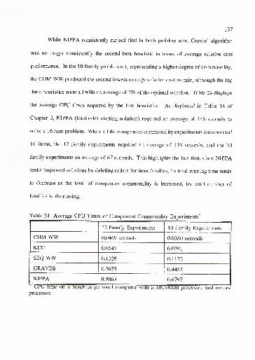
137

While NIPPA consistently ranked first in both problem sets, Graves’ algorithm

was no longer consistently the second best heuristic in terms of average relative cost

performance. In the 10 family problem set, representing a higher degree of commonality,

the CUM WW produced the second lowest average relative cost margin, although the top

three heuristics were all with an average of 2% of the optimal solution. Table 24 displays

the average CPU times required by the five heuristics. As displayed in Table 14 of

Chapter 3, NIPPA (lot-for-lot storting solution) required an average of 146 seconds to

solve a 16 item problem. While all the component commonality experiments incorporated

16 items, the 12 family experiments required an average of 116 .seconds, and the 10

family experiments an average of 87 .seconds. This highlights the fact that, since NIPPA

seeks improved solutions by deleting orders for item families, its total running time tends

to decrease as the level of component commonality is increased, for total number of

families is decreasing.

Table 24 Average CPU Times of Component Commonality Experiments*

12 Family Experiments 10 Family Experiments

CUM WW 0.0469 seconds 0.0380 seconds

KCC 0.0547 0.0391

SEQ WW 0.1328 0.1172

GRAVES 0.5625 0.4453

NIPPAW—/ ' n 1 t X .

—!—n m0.9063 0.6797

CPU time on a MacPIus personal computer with a MC68{)()() proce.ssor and no co-

processor.

138

5.4 Conclusions

Like the Stage Two experiments of Chapter 3, the .scope of the component

commonality experiments, in terms of the variety of "improved" heuristics studied, is

broader than any available in the literature surveyed in Chapter 2. The 16 item Stage

Two experiments (the results of which are displayed in Table 9) can be viewed as the "16

family" companion problem set to the experiments in this chapter, for they utilize the

same product structures, demand patterns, and cost generation scliemes. Comparison of

these results suggests that the presence of component commonality has little effect on

NIPPA’s average performance, because its average relative cost ratio ranges from 1.01

for the 16 family and the 10 family problem sets, to 1.012 for the 12 family problem sets.

The impact of common components within a product structure appears to be greater of

the simpler CUM WW rule, whose relative cost ratio fell from 1.049 for the 16 family

problems of Chapter 3, to 1.025 for the 12 family problems, to 1.015 for the 10 family

problems. These observations are consistent with the recent study of Sum, Png, and Yang

[87], who observed that simpler planning heuristics narrowed the margin of performance

between themselves and an "improved" heuristic (the only such heuristic included in their

study was KCC/BK) as the degree of commonality increases. One po.ssible interpretation

of this observed phenomena is that, given that a heuristic procedure is designed to address

component commonality, increasing the number of common components actually

decreases the underlying complexity of the problem.

CHAPTER 6

HEURISTIC PROCEDURES FOR MULTIPLE STAGE PRODUCTION PLANNINGPROBLEMS WITH JOINT COSTS AND CAPACITY CONSTRAINTS

6,1 Intnxiiiction

While the presence of common components may be one of the most familiar forms

of joint costs that may arise in multiple stage production planning, it is not generalized

enough to model many other types of Joint costs that may be encountered in a production

system. This is primarily due to the fact that two items do not necessarily need to be

physically identical to share a common ordering cost. Production planning involving

transportation provides a good example of this: two or more items may trigger an

expense if any one or more of them is ordered from a particular supplier. Unlike the

common component case, each item within the supplier Joint cost family may possess a

different inventory holding cost. These items may also each possess individual re-

stocking costs, demonstrating that in the most generalized Joint cost problem, an item may

belong to more than one ordering cost family (for example, see Roundy [7S]). The

integration of production and distribution planning, or "supply chain management", can

require such a highly generalized model of Joint costs, to model widely dispersed

production facilities and customer markets. Where once the problems associ<ated with

heavy manufacturing, assembly, product customization, and distribution pl.inning were

often investigated separately (such as the assembly style problems of Chapter 3), recent

139

140

trends in production and distribution have prompted some practitioners to adopt a wider

scope. Corey Billington [16], manager of Strategic Planning and Modeling at Hewlett-

Packard, stated, "managers must assess the supply chain in its entirety, not just the sum

of its various parts. It’s not just a big picture; it’s the whole picture" (p. 21). Adopting

a more generalized definition of joint costs makes it possible to model entire supply

chains as multiple stige planning problems.

In this chapter of the investigation, we will model two systems incorporating

generalized joint costs. The smaller system was created from the global

production/distribution problem described by Billington and others [16][66][67], while the

larger system models an existing production plant which produces glass bottle storage

systems. Modeling of the larger system introduces another issue, which has not been

addressed in Chapters 3 through 5 of this investigation. As discussed in Chapter 2,

practitioner oriented literature suggests that most existing multiple stage production

systems require the use of limited resources. In this investigation, such limitations are

referred to as capacity constraints. Such capacity constraints will be incorporated into

both systems modeled in this chapter, by transforming the joint cost family into the joint

resource family. Just as in Chapter 5, production of at least one item within a joint

resource family in a particular period triggers a family ordering cost. But now,

production of at least one of the members of a joint resource family also represents

consumption of that resource, whose availability may be limited in that period. Although

items may belong to more than one joint resource family and items within a joint resource

family may consume the resource at different rates, the leadtimes on production of all

141

items within a joint resource family must be assumed constant and identical to the

leadtimes of fellow members. This assumption will allow us to assume leadtimes are

zero, without further loss of generality.

The intention of this framework is to create one modeling methodology that can

be used to describe as many of the diverse multiple stage problems already existing in the

literature as possible. The non-joint cost problems of Chapter 3 can be thought of as

problems in which each item is the sole member of one resource family, and the resource

itself is unlimited. Likewise, the component commonality problems of Chapter 5 can be

modeled as items which each have membership in only one family, although they may

not be the sole member of that family. Items within a family must all have identical

holding costs, for they are actually the same physical component. The coordination of

multiple items unrelated with the exception of a mutual dependence on a limited re.source,

such as the problems studied by Ei.senhut [38], Lambrecht and Vanderveken [63] and

others, can be modeled as items unrelated by parent/child relationships but sharing mutual

membership in one joint resource family with finite resource availability and a joint

ordering cost of zero. If the problem assumes only one c.ipacitated workcenter in a job

shop, .such as the experiments of Sum and Hill [86], the items processed at that

workcenter would all be members of the joint resource family representing that

workcenter. In the case of studies such as Biggs [13], if capacity is interpreted as some

overall limitation on production activity, all items throughout the multiple stage problem

are members in the joint re.source family repre.senting that limitation. The supply chains

142

described by Billington [16] and others can be modeled as a network of resource families,

through which items are transferred and transformed in varying traffic patterns.

NIPPA can be applied to this highly generalized problem. The next section will

describe the computations necessary under the conditions of capacity constraints, and

provide a small example. A description of the two systems mentioned above follows, for

these systems will be used to provide some insight into NlPPA's effectiveness in this

environment. The lower bounds found on the optimal solutions to these problems have

been found through the technique described in Chapter 7.

6.2 The Non-sequential Incremental Part Period Aliiorithm fNIPPA)

6.2.1 An informal description of the use of NIPPA with capacity constraints

As first stated in Chapter 3, NIPPA develops a solution by eliminating orders from

a given schedule, based on the ratio of costs incurred to costs saved by such an

elimination. This decision rule does not change with introduction of capacity constraints.

However, the computations involved in the calculation of these ratios grows more

elaborate under these conditions.

The following section provides a formal outline of the NIPPA procedure in a joint

re.source environment, and the bulk of the instructions concern calculating the effect of

eliminating any particular order. In an environment with unlimited resources, elimination

of an order simply implied incorporating that order and the orders of any necessary

predecessors in that period into their respective neighboring prior production periods.

Now, elimination of an order may require that the order's production be distributed over

several earlier periods, dependent on resource availability. Rescheduling of the order’s

143

predecessors may be likewise complicated. However, NlPPA’s definition of a solution

"neighboring" the current schedule remains essentially unchanged from prior chapters:

the order for one joint resource family has been eliminated from a particular period, and

the production of the items within that fiimily in that period has been distributed across

the earliest existing production periods for which the necessary resources are available.

An eligible production period is one in which an order exists for every joint resource

family to which an item belongs (recall that an item may belong to more than one joint

resource family). Orders for all necessary predecessors to the target joint resource order

have been likewise eliminated. Ratios representing infeasible order eliminations

(sufficient resources do not exist to make the above changes) are discarded.

One complication that arises from capacity constraints is the generation of a

feasible starting solution. The recommended starting solution for NIPPA is lot-for-lot,

but there is no guarantee that such a solution will not contain one or more capacity

constraint violations. One approach to creating a feasible starting solution is to generate

a lot-for-lot solution and assess its resource requirements. If the solution contains periods

in which one or more resource requirements exceeds resource availability, reduce the

orders for items within the offending re.source families, rescheduling these amounts in

earlier periods, as resource availability permits. Dependent on the items in question,

rescheduling of necessary predecessors may also be required.

If the lot-for-lot solution contains numerous violations of re.source availability,

deriving a feasible starting solution through the informal revision method described above

could grow quite cumbersome. As an alternative, the LP relaxation of this prolilem could

144

be solved, using the formulation outlined in section 7.2.2. Rounding all fractional values

for the binary ordering variables up to one will yield a feasible .solution from which

to begin the NIPPA search. Given that a feasible starting solution has been secured, all

revisions implemented by NIPPA will be feasible with respect to all the problem’s

constraints.

6.2.2 Formal statement of NIPPA with capacity constraints

Let CONSUMPTION(f,j) be the amount of resource f required to make one unit of item

j-

Let {Fj} be the set of all resource families for which C0NSUMPT10N(f,j) > 0 for an

item j.

Let {If} be the set of all items for which C0NSUMPT10N(f,j) > 0 for a resource family

f.

Let S|f be the ordering cost incurred if at least one of some item in {If} is ordered in

period i.

Let Cjj be the incremental holding cost incurred by keeping one itemj in inventory during

period i.

Let {Pj} be the set of all nece.ssary predeces.sors of item j.

Let j* be the parent of item j.

Let {Z} be the set of all items which possess a parent.

Let {LEVELf } be the set of all items on the Lth level of the product structure or

structures, where L = 1 is the highest level, consisting of end items.

Let MAXLEVEL be the total number of levels within the "tallest" product structure.

145

Let B" be the solution at iteration n of the NIPPA algorithm.

Let B"(i,j) be the amount of itemj ordered in period i in solution B".

Let BX" be a "copy" of solution B", manipulated with the calculation of each NIPPA

ratio.

Let LOAD"(i,f) =

E CONSUMPTION(fJ)*B\ij) for i = 1, ..., TMIf]

Let LOADX"(i,f) =

E CONSUMPTION(fj)*BX\ij) for z = 1, ..., T

Let CAP(i,f) be the amount of resource f available for use in period i.

Ixt C"(i,j) =

i

Y,B%ij) for i = 1, ..., T and j = 1, ..., Jt=\

Let CX"(i,j) =

i

for i = 1, ..., T and j = 1, .... Jt=\

Let ZEROS"(i,j) = i - t, where period t is the latest period prior to period i, such that

LOAD"(t,f) > 0 for all f in {Fj}. If no such period exists, let ZEROS"(i,j) = -1.


a. Generate a feasible order schedule B", preferably lot-for-lot. If re.source availability

does not permit lot-for-lot, shift production from over burdened periods to some earlier

periods, to create a feasible schedule.

146

b. Compute C“(iJ) and ZEROS"(i,j) for i = 1, T andj= 1, J. Compute LOAD“(i,f)

for i = 1, T and f = 1, N.

c. Let n = 0.

Step 1: Generate ratios.

a. Let t = 2 and f = 1. Let INFEASIBLE(i,g) = 0 for all i = 1, T and g = 1, N.

b. Let NUMERATOR = 0 and DENOMINATOR = 0. If ZEROS"(t,j) = -1 for anyj

in

{If}, let INFEASIBLE(t,f) = 1 and go to substep j.

c. Let BX"(i,j) = B"(i,j) for i = 1, t andj= 1, J.

d. Let CX"(i,j) = C"(i,j) for i = 1, t andj= 1, J.

e. Let LOADX"(i,g) = LOAD"(i,g) for i = 1, t and g = 1, N.

f. For each itemj

in {If}:

i. Let DESTINATION = t - ZEROS"(t,j).

ii. Let BX"(DESTINATION,j) = BX"(DESTINATION,j) + BX"(t,j).

iii. Calculate LOADX"(DESTlNATION,g) for g =

iv. Let TIGHTEST = MIN{(CAPg - LOADX"(DESTINATION,g)) /

CONSUMPTION(j,g)I g is a member of {Fj} }.

V. Let NUMERATOR = NUMERATOR + Cij*BX"(t,j)*ZEROS"(t,j).

vi. Let BX"(t,j) = 0.

vii. If TIGHTEST > 0, return to substep f.i and repeat for the next itemj in {If}.

If this process has been completed for all itemsj in {If}, then go to substep g.

viii. If DESTINATION = 0, let INFEASlBLE(t,f) = 1. Go to substep j.

xi. Let BX"(DESTINATION,j) = BX"(DESTlNAT10N,j) + TIGHTEST.

147

X. Let DESTINATION = DESTINATION - ZEROS"(DESTINATION,j).

xi. If ZEROS"(DESTINATION,j) = -1, let INFEASlBLE(t,0 = 1. Go to substep

j-

xii. Let NUMERATOR = NUMERATOR - (TIGHTEST *Cij

*

ZER0S"(DESTINAT10N,j)).

xiii. Let BX"(DESTlNATION,j) = BX"(DESTINAT10N,j) - TIGHTEST. Return

to substep f.iii.

g. Calculate CX"(i,j) for i = 1, t andj= 1, J. Let L = 2.

h. For each itemj

in {LEVEL, }:

i. Let i = t - 1.

ii. If CX"(i,j) < CX"(i,j*), then let NUMERATOR = NUMERATOR +

c,T(CX"(i,j*) -CX"(i,j)).

iii. If CX"(i,j) < CX"(i,j'), then let CX"(iJ) = CX"(i,j‘).

iv. If CX”(i-l,j) < CX"(i,j) and LOADX"(i,g) = 0 for at least resource family g

in {Fj}, then let NUMERATOR = NUMERATOR + cij*(CX"(i,j) - CX"(y,j)) for y = i-

ZEROS"(i,j) to i-1. Let CX"(y,j) = CX"(i,j) for y = i - ZEROS"(i,j) to i. If ZEROS"(i,j)

= -1, then let INFEASIBLE(t,f) = 1 and go to step j.

V. Let i = i - 1. If i > 0, go back to substep h.ii.

vi. Let BX"(1J) = CX'XLj) forj= 1, ... J. Let BX"(i,j) = CX"(i,j) - CX"(i-lJ) for

i = 2, ..., T andj= 1, ..., J.

vii. Calculate LOADX"(i,g) for i = I, ..., t and g = 1, ..., N.

viii. Let DESTINATION = t-1.

148

ix. Let TIGHTEST = MIN{(CAP^ - LOADX"(DESTINATION,g)) /


X. If TIGHTEST > 0, let DESTINATION = DESTINATION-1. If, as a result,

DESTINATION = -1, return to substep f.i and repeat for the next itemj

in LEVELl. If

DESTINATION = -1 and the process has been completed for all items in LEVELl, go

to substep f.xvii. Otherwise, return to substep f.v.

xi. If t = 0, let INFEASIBLE(t,f) = 1. Go to step j.

xii. If ZEROS"(DESTINATION,j) = -I, let INFEASlBLE(t,f) = 1. Go to step j.

xiii. Let BX"(DESTINATION,j) = BX"(DESTINATION.j) + TIGHTEST.

xiv. Let DESTINATION = DESTINATION - ZEROS"(DESTINATION,j).

XV. Let BX"(DESTINATION,j) = BX"(DESTINATION,j) - TIGHTEST.

xvi. Let NUMERATOR = NUMERATOR - (TIGHTEST * 0,^

*

ZEROS"(DESTINATION,j)). Return to substep f.v.

xvii. Let L = L + 1. If L MAXLEVEL, go back to substep i.

h. Calculate order cost savings.

i. Calculate LOADX„(t,g) for g = 1, ..., N.

ii. If LOADX"(t,g) = 0 and LOAD(t,g) > 0, then DENOMINATOR =

DENOMINATOR + S;g, for g = 1, ..., N.

i. Let RATIO"(t,f) = NUMERATOR/DENOMINATOR.

j. Let = t = t + 1. If t > T, then let t = 2 and f = f + 1. If f < N, go to substep b.

k. Find LOWRATIO"(LOWPERIOD,LOWFAMlLY) = MIN {RATIOSn(i,g)|

INFEASIBLE(i,g) = ()}.

149

Step 2:

If LOWRATIO"(LOWPERIOD,LOWFAMILY) > 1, go to Step 4. Otherwise, go to Step

3.

Step 3: Generate new solution.

a. For each itemj

in {Ilowfamily}-

i. Let DESTINATION = LOWPERIOD - ZEROS"(LOWPERIOD,j).

ii. Let B"(DESTINATION,j) = B"(DESTINAT10N,j) + B"(x,j).

iii. Calculate LOAD"(DESTINATION,g) for g = 1,...,N.

iv. Let TIGHTEST = M1N{(CAP^ - L0AD"(DESTINAT10N,g)) /

CONSUMPTION(j,g)I g is a member of {Fj}

}

V. Let B"(L0WPER10D,j) = 0.

vi. If TIGHTEST > 0, return to substep a.i and repeat for the next itemj

in

{Ilowfamily}- If this process has been completed for all itemsj

in {1 |,owfamily}’ go to

step b.

vii. Let B"(DESTlNAT10N,j) = B"(DESTlNAT10N,j) + TIGHTEST.

viii. Let DESTINATION = DESTINATION - ZER0S"(DESTINAT10N,j).

iv. Let B"(DESTINAT10N,j) = B"(DESTlNATION,j) - TIGHTEST. Return to

substep a. iii.

b. Calculate C"(i,j) for i = 1, ..., x andj= 1, L Let L = 1.

c. For each item in {LEVEL, }:

i. Let i = X - 1.

ii. If C"(i,j) < C"(i,j*), then let C"(i,j) = C"(i,j*), for i = 1 T andj= 1, ..., J.

150

iii. If C"(i-l,j) < C"(i,j) and LOAD"(i,g) = 0, then let C"(y,j) = C"(i,j) for y = i-

ZEROS"(i,j) to i.

iv. Let i = i - 1. If i > 0, go back to substep c.ii.

V. Let = C'XLj) forj= 1, ... J. Let B"(i,j) = C"(i,j) - C"(i-l,j) for i = 2,

..., T andj= 1, ..., J.

V. Calculate LOAD"(i,g) for i = 1, ..., LOWPERIOD and g = 1, N.

vi. Let DESTINATION = LOWPERIOD-I

.

vii. Let TIGHTEST = MIN{(CAPj, - LOAD"(DESTINATION,g)) /


viii. If TIGHTEST > 0, let DESTINATION = DESTINATION-1. If

DESTINATION = -1, return to substep i and repeat for the next itemj

in LEVELl- If

DESTINATION = -1 and the process has been completed for all items in LEVELl, go

to substep c.xii. Otherwise, return to substep c.vii.

ix. Let B"(DESTINATION,j) = B"(DESTlNAT10N,j) + TIGHTEST.

X. Let DESTINATION = DESTINATION - ZEROS"(DESTINATION,j).

xi. Lei B"(DESTINATION,j) = B"(DESTINATION,j) - TIGHTEST.

xii. Let L = L -I- 1. If L^ MAXLEVEL, go back to substep c.i. Repeat process

for all itemsj in {LEVEL}l.

d. Compute C"(i,j) and ZEROS"(i,j) for i = 1, ..., T andj= 1, ..., J. Compute LOAD"(i,f)

for i = 1, ..., T and f = 1, ..., N.

e. Let n = n + 1.

f. Go back to Step 2.

151



6.2.3 An example

Consider the following example of a 4 period multiple stage planning problem

with a simple two item product structure: let item A be the parent item with an

incremental holding cost of $2.5 per unit per period, and let item B be the child item,

with an incremental holding cost of $5. External demand for end item A is 1 for the first

period, 3 for the second period, 7 for the third period, and 3 for the fourth period. While

the problem contains only two items, it also contains three resource families:

Amount Required Amount Required Total Resource Family

To Produce To Produce Available Order

Family One Item A One Item B per Period Cost

1 1 0 20 $1002 0 1 20 $2003 3 2 31 $50

We begin by creating a feasible starting solution. Begin with a lot-for-lot solution

and compute LOAD0(i,g) for i = 1, ..., 4 and g = 1, ..., 3.

LOT-FOR-LOT SOLUTION: LOAD:Period: 1 2 3 4 Period: i 2 3 4

j= "A" 1 3 7 3 Family 1 1 3 7 3

j= "B" 1 3 7 3 Family 2 1 3 7 3

Family 3 5 16 35 15

A review of the LOAD table shows that a strict lot-for-lot .solution is not feasible,

because the requirements made of resource family 3 exceeds the resource available in

period 3 by the amount of 4. At this point, we shift this excess requirement into the next

earliest period (or period.s) for which production of this amount would be feasible. In this

152

case, the relocation of one item A and one item B from production in period 3 to

production in period 2 produces a feasible starting solution:

STARTING SOLUTION (B“):

Period: 12 3 4

LOAD":Period: 1 2 3 4

j= "A" 1 4 6 3 Family 1 1 4 6 3

j= "B" 1 4 6 3 Family 2 I 4 6 3

Family 3 5 20 30 15

At this point, we calculate RAT10'’(i,f) for i = 2 through 4 and f = 1 through 3.

For example, elimination of an order for family 1 in period 2 requires that the production

of its sole member A be shifted to the first period. This shift is performed on a copy of

the current schedule, and the resulting resource requirements are calculated. (This

modified copy of the current solution is referred to as BX” and its load table is referred

to as LOADX”, to remind us that neither represents that actual solution at this iteration.)

BX":

Period: i 2 3 4

LOADX":Period: 1 2 3 4

j= "A" 5 0 6 3 Family 1 5 0 6 3

j= "B" 1 4 6 3 Family 2 1 4 6 3

Family 3 17 8 30 15

Period 1 is referred to as DESTINATION in section 6.2.2, and now we review all

families of which item A is a member, to identify which has the least resource slack in

the DESTINATION period. This slack, stated in terms of the number of item A’s which

could be produced with it, is referred to as the variable TIGHTEST in section 6.2.2. In

the ca.se of this example, TIGHTEST equals the minimum of (20-5)/l and (31-17)/3, or

4.667. Since TIGHTEST > 0, the shift of item A is considered complete.

NUMERATOR, initially equal to zero, is now increased by the cost incurred by this shift:

NUMERATOR = NUMERATOR + (2.5* 1*4) = 10.

153

At this point, the schedules of any of A’s immediate predecessors may need

adjustment to maintain feasibility. To facilitate this feasibility check, the revised schedule

is restated in terms of cumulative production:

CX°:

Period: J. 2 3 4

j= "A" 5 5 11 14

j= "B" 1 5 11 14

Beginning with the second highest level in the product structure, if the cumulative

production of any item is le.ss than its parent, then its cumulative production is increased

to the level of its parent. In this example, the cumulative production of item B would be

increased to 5 in the first period. The revised cumulative production schedule is then

translated back to the per period production schedule BX”, and the LOADX” table

likewise updated.

BX”: LOADX”:Period: i 2 3 4 Period: 1 2 3 4

j= "A" 5 0 6 3 Family 1 5 0 6 3

j= "B" 5 0 6 3 Family 2 5 0 6 3

Family 3 25 0 30 15

The revised schedule is feasible with respect to resource requirements and does

not imply shifting production of item B into a period in which .some production does not

already exist on the current schedule. Either condition, had it been present, would have

required further revision or declaration of this order elimination as infeasible. The

numerator, however, must be increased to reflect the costs incurred by revising item B’s

schedule: NUMERATOR = NUMERATOR + (5*1*4) = 10 + 20 = 30. Now all that

remains to complete the ratio is calculation of the denominator. This is done by

comparing schedule LOADX” to the "true" current resource load table LOAD”:

LOAD":Period: i 2 3

LOADX°:4 Period: 1 2 3 4

Family 1 1 4 6 3 Family 1 5 0 6 3

Family 2 1 4 6 3 Family 2 5 0 6 3

Family 3 5 20 30 15 Family 3 25 0 30 15

If, for any family f in period 2, LOAD"(f,2) > 0 and LOADX"(f,2) = 0,

DENOMINATOR = DENOMINATOR + S|f. Inspection of the two tables above shows

this is true for all three families, so DENOMINATOR = 100 + 200 + 50 = 350. Thus,

RATIO“(2,l) = 30 / 350 = 0.0857. At this point, we reset NUMERATOR and

DENOMINATOR to zero, reset BX”, CX”, and LOADX" to the values of B®, C“ and

LOAD”, and begin this process again for the next ratio. When the ratio calculation

process is finished for all orders eligible for elimination, we have the following ratio

table:

RATIOS”:

Period: i 2 3 4Family 1 X 0.0857 0.2214 0.1571

Family 2 X 0.1000 0.1750 0.1500

Family 3 X 0.0857 0.1857 0.1286

On this table, there is a tie for low ratio, which is broken in favor of the family

with the most members. Therefore, LOWRATIO”(LOWPER10D,LOWFAMILY) =

0.0857, with LOWPERIOD = 2 and LOWFAMILY = 3. Since LOWRATIO" > 1, we

proceed to iteration 1.

Iteration 1.

LOWPERIOD - 2 and LOWFAMILY = 3 implies that all production of family

3 members (and their necessary predecessors) in period 2 must be eliminated, and

155

rescheduled in the next earliest production periods. The result is current schedule B*, and

accompanying resource requirement table LOAD':

B': LOAD':Period: J 2 3 4 Period: 1 2 3 4

j= "A" 5 0 6 3 Family 1 5 0 6 3

j= "B" 5 0 6 3 Family 2 5 0 6 3

Family 3 25 0 30 15

Now, order elimination ratios are calculated, based on the .schedule B':

RATIOS':

Period: i 2 3 4

Family 1 X X 1 1

Family 2 X X 1 0.225

Family 3 X X 1 1

Note that, although orders exist for families 1,2, and 3 in period 3 and families 1

and 3 in period 4, sufficient resources are not available at earlier order periods to shift

production out of these periods. Thus, an "I" appears in the table to denote an order that

cannot be eliminated due to infeasibility. LOWRAT10'(LOWPERIOD = 3,

LOWFAMILY = 2) = 0.225 is also the only eligible ratio in this ca.se.

Iteration 2.

Now all the production of family 2 is shifted from period 4 into the next earliest

order periods with availlable capacity:

B-:

Period: i 2 3 4

LOAD-:Period: 1 2

j= "A" 5 0 6 3 Family 1 5 0

j= "B" 8 0 6 0 Family 2 8 0

Family 3 31 0

1 4

6 3

6 0

30 9

156

Now there exists no more orders eligible for elimination, so the algorithm

terminates here. Schedule is the proposed order schedule, with a total cost of $1032.5.

The cost of the feasible starting solution, in contrast, was $1,407.5.

6.3 An Evaluation of NlPPA’s Application to Multiple Stage Planning Problems with

Joint Costs and Capacity Constraints.

6.3.1 Introduction

To test the application of NIPPA to highly generalized multiple stage problems

such as those required by such models as supply chain management, two experiment sets

were created. The first set represents a simplified supply chain system, while the larger

second set was modeled after an existing production facility. In the case of all

experiments, a lower bound on the optimal solution was found for comparison, using the

Lagrangian relaxation method discussed in Chapter 7.

6.3.2 The Supply Chain Experiment Set

The supply chain experiments, modeled after the global manufacturing and

distribution problems described by Billington [16] and others, involve 20 items scheduled

acro.ss 20 periods of demand. Each item belongs to exactly one of 9 joint resource

families. Figure 20 illustrates the overall pattern of flow of inventory between families,

while Figure 21 shows the specific product structures into which the 20 items are

embedded. The relationship between the families in Figure 20 and the items in Figure

21 are displayed in Table 25. If an item belongs to a family, it is assumed to require one

unit of the family resource to produce one unit of the item.

157

FLOW OF INVENTORY

figure 20 Supply Chain Experiment Family Structure

"igure 21 Supply Chain Experiment Product Structures

158

Table 25 Family/Item Relationships of the Supply Chain Experiments

Family Name Total Resource Available

Each Period

Items Which are

Members of Family

1 1450 C, H, and N

2 1450 D, I, and O

3 1150 P and T

4 1450 B, G, and L

5 1150 M and S

6 1450 F , K, and R

7 1000 A

8 450 E and J

9 1000 0

External demand requirement patterns for end items A and Q were generated

randomly from a uniform distribution ranging from 0 to 500, while the range of the

uniform distribution used to generate external demand patterns for item E was from 0 to

150, and the range for end item J from 0 to 75. The lot-for-lot solutions resulting from

each set of demand requirements were .screened for feasibility with re.spect to all family

resources. If an infeasibility was detected in a particular lot-for-lot starting solution, an

appropriate end item demand requirement was reduced in the offending period, and

increased in the earliest periods in which resource capacity was available. (Such

infeasibilities were slight and infrequent in the lot-for-lot solutions, due to the specified

levels of resources available.) A total of ten starting solutions were created.

One set of incremental holding costs was generated for the 20 items, from a

uniform(0,l) distribution. Two sets of family ordering costs were generated in a similar

159

fashion, one from a uniform(0,500) distribution and one from a uniform(0,1000)

distribution. The two sets of ordering costs combined with the ten demand patterns

resulted in 20 experiments. The expected family ordering cost of one problem set is

twice that of the other, implying that order cycles within tho.se schedules, on average,

would be twice as long. But longer order cycles also implies larger orders, which implies

higher resource consumption within certain order periods.

6.3.3 Supply Chain Experiment Results

The set of 10 problems with the uniform(0,500) family order cost .set will be

referred to as Set One and the remaining 10 problems (with the uni form (0,1 000) family

order cost set) will be referred to as Set Two. In the ca.se of each problem, a lower

bound on the optimal solution was found using the method described in Chapter 7.

Tables 26 and 27 display the results.

Table 26 Results of Supply Chain Experiment Set One

Problem

Number

Cost of

Starling

Solution

Cost of

NIPPA

Solution

l^rwer Bound

on Optimal

Cost

Starling Solution/

NIPPA Cost

Ratio

NIPPA/ I^wer

Bound Cost

Ratio

NIPPA CPUTime*

1 44260 32818.9 29877.8 1.3486 l.(»S4 129.0

2 44260 33210.8 28503.2 1.3327 1.1652 142.7

3 44260 34747.3 29818.5 1.2738 1.1653 143.6

4 44260 30644 26972.6 1.4443 1.1361 158.9

5 44260 34915.9 31076.2 1.2676 1.1236 133.0

6 44260 31548.1 29102.6 1.4029 1.0840 132.1

7 44260 34203.6 29743.5 1.2940 1.1500 140.2

8 44260 32510.6 29486.9 1.3614 1.1025 133.1

9 44260 33179.3 29137.2 1.3340 1.1387 151.8

10 44260 32721.6 28844.2 1.3526 1.1344 145.7

Average:

* /^rST T

1.3412 1.1293 141.0

CEU time is in seconds on an EVEKEX 486/33 with math co-processor.

160

Table 27 Results of Supply Chain Experiment Set Two

Problem

NumberCost of

Starting

Solution

Cost of

NIPPASolution

Lower

Bound on

Optimal

Cost

Starling

Solution/

NIPPACost

Ratio

NIPPA/

Lower

Bound

Cost

Ratio

NIPPACPUTime*

1 87960 51583.4 45125.1 1 .7052 1.1431 180.8

2 87960 50883.4 44131.2 1.7287 1.1530 183.0

3 87960 49959.2 46023.9 1.7606 1 .0855 173.7

4 87960 44792.6 41381.9 1.9637 1 .0824 188.1

5 87960 52677.6 48756.2 1.6698 1 .0804 174.6

6 87960 47927.2 44695.5 1.8353 1.0723 174.6

7 87960 49527.5 45625.8 1.7760 1 .0855 175.4

8 87960 53038.4 46843.3 1 .6584 1.1323 183.6

9 87960 49801.4 46006.6 1.7662 1 .0825 185.8

10 87960 49797.1 44388.8 1.7664 1.1218 177.4

Average: 1 .7630 1.1039 179.7

CRU time is in seconds on an EVEKEX 4X(i/33 with math co-processor.

NIPPA, on average, found solution that were at most within 12.9% of the optimal

solution for Set One and 10.4% for Set Two. The lower bound finding .scheme, outlined

in Chapter 7, most likely does not find bounds as tight as tho.se utilized in Chapters 3 and

5. In addition, it is not known if the tightness of these bounds (that is, their distance from

the optimal solution’s total cost) is consistent across all problems. Therefore, it would

be unwise to compare NlPPA’s relative cost ratios of Chapters 3 and 5 with the.se results,

due the bounding schemes. It does confirm, however, that NlPPA's .solutions were within

an average of, at most, approximately 11% of optimal, ranging from as close as 7.2%

to as much as 16.5% when reviewed on a problem by problem basis. Since there exists

161

no other procedure reviewed in the literature survey of Chapter 2 that addresses such a

generalized problem as this, the only other solution available for comparison in this

investigation is the feasible starting solution. In the case of Set One, the les.ser family

ordering costs, NIPPA produced a 34% improvement over its starting solution, on

average. For Set Two, in which the average family ordering cost was doubled, NIPPA

produced a 76.3% improvement over the starting solution.

6.3.4 Bottle Racking Experimental Design

This .set of experiments models an existing plant which produces storage racks for

glass bottles of various sizes. The system produces six end items, which result from the

combination of two different heights and three different depths of racks. Modeled, the

system involves 17 re.source familie.s, which are illustrated in Figure 22. Families 2, 8,

9,10 and 17 represent the activation of work centers, at which there is a limited amount

of machine capacity available. Families 3, 4, 5, 6, and 7 represent set ups for various

types of components requiring the machinery of the family 2 workcenter. This is an

example of the most generalized form of joint costs and resources, where an item may

belong to more than one family. An order for an item in family 3, for example, will

incur the cost for the family 3 set up, incur the cost for the activation of the workcenter

in which this type of production resides, and be bounded by the overall machine hours

available at the workcenter and perhaps by .some constraint on making family 3 member

items in particular. There is a total of 78 items in the bottle racking experimental design,

and their parent/child relationships are illustrated in Figure 23.

162

A FINISHED GCX)DS A

Family 14: Family 15: Family 16:

Single Depdi Double Depth Magnum DepthAssembly Assemhly Assembly

k

FLOW OF INVENTORY

Family iTSingle Depth

tfitcz Pnxhidicxi

Double Depth^ter PToductian

Family iSVlagmim Depth

] ifiter Ptoductlali

Family 10: J^ter Piece Production Oeal

%

Family 8:

Rip SawProduction

Center

Family 9: Miter

Piece Prep Center

Famify 3;

20 Bottle

HighVertical

Production

Family 4:

24 Bottle

HighVertical

Ptoductlan

Family 5:

Single

Depth

Cross-Cut

Production

Family 6;

Double

Depth

Cross-Cut

Production

Family 7:

MagnumD^th

Cross-Cut

Production

Family 2: Cross-Cut Production Center 4FLOW OF INVENTORY

Family 1:

Receipt of RawMaterials

Mgure 22 The Resource Families of the Bottle Racking Experiments

Items P, Q, R, S, T, and U are the end items, representing 20 and 24 bottle high

storage columns of single, double, and magnum depth racks. Items with matching letters

in their labels represent common components, revealing an high degree of component

163

Figure 23 Product Structures of the Bottle Racking Experiments

commonality in this system. While there are 78 items produced, there are only 15 distinct

products or parts. However, this is not component commonality in the strictest sen.se, for

common parts are required in different amounts by different product structures. Thus, the

item denotes not just what part is required, but how much of that part is required in that

application, implying varying holding costs and resource consumption rates across the

various occurrences of that part requirement. Table 28 relates the items to the resource

families, while Table 29 provides more detailed information concerning each of the 78

items.

164

Table 28 Family/Item Relationships in the Bottle Racking Experiments

Family Name Total

Resource

Available

per Period

Items Which are Members of Family Family

Ordering

Cost

1: Raw Materials 3500 A1-A2, B1-B20 500

2: Cross-cut

Workcenter

1200 C1-C3, D1-D3, E1-E4, F1-F6, G1-G6 50

3: 20 Bottle High

Vertical Cut Set Up200 C1-C3 15

4: 24 Bottle High

Vertical Cut Set Up200 D1-D3 15

5: Single Depth Cut Set

Up500 E1-E4 15

6: Double Depth Cut

Set Up500 F1-F6 15

7: Magnum Depth Cut

Set Up500 G1-G6 15

8: Rip Saw Workcenter 1200 H1-H2, 11-16, J1-J4 50

9: Miter Prep

Workcenter

2000 K1-K4, L1-L2 5

10: Miter Qit

Workcenter

1500 M1-M2, N1-N2, 01-02 10

11: Single Depth Miter

Production

1500 M1-M2 25

12: Double Depth Miter

Production

1000 N1-N2 25

13: Magnum Depth

Miter Production

1000 01-02 25

14: Single Depth Rack

Assembly

40 P, 0 50

15: Double Depth Rack

Assembly

40 R, S 5

16: Magnum Depth

Rack Assembly

20 T, U 5

17: Rack Assemby

Workcenter

100 P, Q, R, S, T, U 2

165

Table 29 Detailed Description of Bottle Racking Items and Respective Resource

Requirements

Name of

Item(s)

Description Resource Consumption

Rate(s)

(The Amount the

Family Resource

Needed to Create Oneof the Item)

Per Unit,

Per Period

Incremental

Holding

Cost

A1 ,A2,

and A3Raw material destined to

become 24 bottle high

verticals

16 of family resource 1 0.48

B4, Bll,

and B18

Raw material destined to

become 20 bottle high

verticals


B1 and B5 Raw material destined to

become single depth column

cap


B8 and

B12Raw material destined to

become double depth column

cap


B15 and

B19Raw material destined to

become magnum depth

column cap


B2 Raw material destined to

become 24 bottles worth of

single depth square pieces




single depth square pieces




single depth miter pieces




single depth miter pieces


166

Table 29 Continued

Name of

Item(s)


Rate(s)

(The Amount the

Family Resource


Per Unit,

Per Period

Incremental

Holding

Cost



double depth square pieces




double depth square pieces


BIO Raw material destined to


double depth miter pieces




double depth miter pieces




magnum depth square pieces

7.5 of family resource

1

0.0225



magnum depth square pieces




magnum depth miter pieces

27 of family resource 1 .0675



magnum depth miter pieces


]

0.0675

Cl,C2,

and C324 bottle high verticals 1 of family resource 2

and

1 of family re.source 4

0.5

Dl, D2,

and D320 bottle high verticals 1 of family resource 2

and

1 of family resource 4

0.5

167

Table 29 Continued

Name of

Item(s)


Rate(s)

(The Amount the

Family Resource


Per Unit,

Per Period

Incremental

Holding

Cost

El and E3 Single Depth Column Cap 1 of family resource 2

and


0.5

E2 Single depth cross cuts

destined to become 24

bottles worth of single depth

square pieces


and


0.25

E4 Single depth cross cuts



square pieces


and


0.2

FI Double depth cross cuts



miter pieces


and


0.54

F2 Double depth cross cuts



miter pieces


2 and


0.45

F3 and F6 Double Depth Column Cap 1 of family resource 2

and

1 of family re.source 6

0.5



bottles worth of double depth

square pieces


and


0.25




square pieces


and


0.2

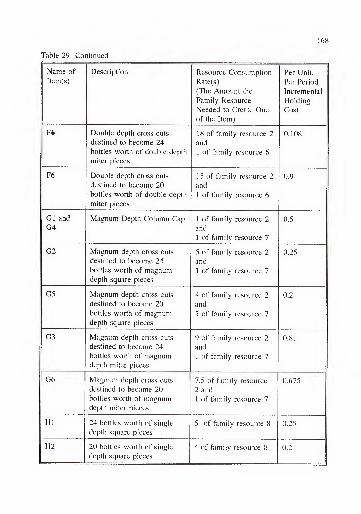
168

Table 29 Continued

Name of

Item(s)


Rate(s)

(The Amount the

Family Resource


Per Unit,

Per Period

Incremental

Holding

Cost




miter pieces


and


0.108




miter pieces


and


0.9

G1 and

G4Magnum Depth Column Cap 1 of family resource 2

and


0.5

G2 Magnum depth cross cuts


bottles worth of magnumdepth square pieces


and


0.25



bottles worth of magnumdepth square pieces


and


0.2



bottles worth of magnumdepth miter pieces


and


0.81





2 and


0.675

HI 24 bottles worth of single

depth square pieces


H2 20 bottles worth of single

depth square pieces


169

Table 29 Continued

Name of

Item(s)


Rate(s)

(The Amount the

Family Resource

Needed to Create One

of the Item)

Per Unit,

Per Period

Incremental

Holding

Cost

11 Double depth squares



miter pieces





miter pieces

7.5 of family re.source

8

0.75

13 24 bottles worth of double

depth square pieces


15 20 bottles worth of double

depth square pieces





miter pieces

18 of family re.source 8 0.18




miter pieces


J1 24 bottles worth of magnumdepth square pieces


8

0.25

J3 20 bottles worth of magnumdepth square pieces


J2 Magnum depth squares




170

Table 29 Continued

Name of

Item(s)


Rate(s)

(The Amount the

Family Resource


Per Unit,

Per Period

Incremental

Holding

Cost

J4 Magnum depth squares




8

0.1125

K1 Prepped double depth

squares destined to become

24 bottles worth of single

depth miter pieces

18 of family resource

9

0.9

K2 Prepped depth squares



miter pieces


9

0.75

K3 Prepped double depth


24 bottles worth of double

depth miter pieces


9

0.9

K4 Prepped depth squares


bottles worth of double

depth miter pieces


9

0.75

LI Prepped magnum depth


24 bottles worth of magnumdepth miter pieces


9

0.9

L2 Prepped magnum depth


20 bottles worth of magnumdepth miter pieces


9

0.75

Ml 24 bottles worth of single

depth miter pieces

1.2 of family 10 and

36 of family 1

1

0.18

171

Table 29 Continued

Name of

Item(s)


Rate(s)

(The Amount the

Family Resource


Per Unit,

Per Period

Incremental

Holding

Cost

M2 20 bottles worth of single

depth miter pieces

1 of family 10 and

30 of family 1

1

0.15

N1 24 bottles worth of double

depth miter pieces

1.2 of family 10 and

36 of family 1

1

0.18

N2 20 bottles worth of double

depth miter pieces

1 of family 10 and

30 of family 1

1

0.15

01 24 bottles worth of magnumdepth miter pieces

1 .2 of family 1 0 and

36 of family 1

1

0.18

02 20 bottles worth of magnumdepth miter pieces

1 of family 10 and

30 of family 1

1

0.15

P A 24 bottle high, single

depth bottle storage column

1 of family 14 and

1 of family 17

0.48

Q A 20 bottle high, single


1 of family 14 and

1 of family 17

0.4

R A 24 bottle high, double


1 of family 15 and

1 of family 17

0.48

S A 20 bottle high, double


1 of family 15 and

1 of family 17

0.4

T A 24 bottle high, magnumdepth bottle storage column

1 of family 16 and

1 of family 17

0.48

U A 20 bottle high, magnumdepth bottle storage column

1 of family 16 and

1 of family 17

0.4

Ten problems were generated, each spanning 12 planning periods. External

demand requirements were generated for each of the six end items (items P through U),

screeened and corrected for initial feasibility in the same manner described in previous

172

sections. Demand for all single and double depth end items was generated from an

uniform(0,20) distribution, while demand for the two magnum depth end items was

generated from a uniform(0,10) distribution. Demand distribution, product structures,

families, and costs were all ba.sed on the existing production facility, with .some .scaling

and random disturbances to disguise the actual data. Leadtime is assumed constant and

identical within the membership of families 1, 2, 8, 9, 10, and 17, .so that it might be

further assumed to be zero for ease of computations. Since time within planning periods

is modeled as a limited resource for most of the families, the assumption of zero

leadtimes between many of the earlier parts making proce.sses (the leadtimes of members

of families 2, 8, 9, and 10) is itself not that far from the actual dynamics of the existing

system. The entire production system was housed within a single facility (in contrast to

the supply chain problems), and smaller transfer batches would frequently be forwarded

to the next workcenter, even as the "order" for that particular item was still in the process

of completion. This nearly simultaneous production of a child and its parent item implies

zero leadtimes, as leadtimes are modeled in this framework. For further discussion of

transfer versus production batches, the reader is referred to Fry, Cox and Blackstone [45].

6.3.5 Bottle Racking Experimental Results

Table 30 displays the results of the 10 bottle racking experiments. The 78 item

schedule developed by NIPPA was, on average, within 9.5% of the optimal schedule.

This margin ranged from as low as within 3.8% up to within 12.6% of the optimal

schedule. As mentioned previously, it is not wise to attempt any further interpretation of

NIPPA’s performance from the.se numbers, because the degree of looseness and the

173

consistency of looseness of these bounds on the optimal solution is not known. When

compared to its feasible starting solution, NIPPA provided, on average, a 62%

improvement of schedule cost.

Table 30 Results of Bottle Racking Experiment Set

Problem

NumberCost of

Starting

Solution

Cost of

NIPPASolution

Lower

Bound on

Optimal

Cost

Starting

Solution/

NIPPA

NIPPA/Lower

Bound

NIPPACPUTime*

1 9924 5936.62 5411.40 1.6717 1.0971 788.0

2 9924 6249.57 5771.66 1.5879 1.0828 565.3

3 9924 6118.93 5895.67 1.6219 1.0379 602.5

4 8792 5769.78 5149.40 1.5238 1.1205 420.2

5 9924 6031.32 5424.51 1 .6454 1.1119 479.1

6 9924 6078.51 5480.89 1 .6326 1.1090 856.6

7 9529 5854.83 5247.26 1.6275 1.1158 342.0

8 9924 6268.70 5715.38 1.5831 1 .0968 340.0

9 9924 6113.93 5431.10 1 .6232 1.1257 377.4

10 9924 5911.69 5641.26 1 .6787 1.0479 588.9

Average 1.6196 1.0945 536.0

* CPU time is in seconds on an EVER EX 486/33 with math co-processor.

6.4 Conclusions

This chapter de.scribed the application of NIPPA to deterministic multiple stage

planning problems complicated by joint costs and a framework of resource limitations as

generalized as any in the literature covered in Chapter 2. NlPPA’s performance was

tested with two sets of experiments, one modeled after supply chain management and one

modeled after an existing production system. In either ca.se, NIPPA found solutions that

174

were, at most, within 9.5% to 12.9% of the optimal solution. The benchmarking of a

heuristic against some bound on the optimal solution to a multiple stage problem with

capacity constraints is itself neglected by the literature, and there is reason to believe that

the bounds utilized here are somewhat loo.ser than tho.se of Chapters 3 and 5. Because

none of the techniques covered previously can be extended to the.se problems in their

stated form, the only other benchmark for gauging NIPPA’s performance is the value of

its starting solutions, which them.selves represent feasible schedules. The computational

effort of NIPPA applied to these capacitated conditions yielded schedules whose costs

ranged from a 26.7% to a 83.9% improvement over the costs of the starting solution.

Given these benchmarks, it can be concluded that NIPPA is a viable method for multiple

stage production planning in a highly generalized multiple limited resource environment.

CHAPTER 7

MATHEMATICAL PROGRAMMING FORMULATIONS AND BOUNDINGPROCEDURES FOR MULTIPLE STAGE PRODUCTION PLANNING PROBLEMS

WITH JOINT COSTS AND CAPACITY CONSTRAINTS

7.1 Introduction

As the degree of generalization is increased in multiple stage production planning,

the computational burden of obtaining optimal solutions can likewise be expected to

increase. However, Chapter 3 demonstrated the merit of obtaining bounds on these

solutions, even when pursuing the solutions themselves is deemed impractical. With

bounds on the optimal solution, greater insight can be gained on the behavior of relevant

heuristics, the necessity of which having been strengthened by the extreme rigors of

optimization. In this chapter we will outline the methods used to find such bounds for

the experiments in Chapters 5 and 7. Similar to the structure of Chapter 4, we begin by

reviewing two mathematical formulations applicable to these experiments. In the

following sections, Lagrangian relaxation techniques based on these formulations are

developed. These techniques were used to find lower bounds on the optimal solutions to

all experiments in Chapters 5 and 6.

175

176

1.2 Problem Formulation

7.2.1 The Binary Formulation with Joint Costs

The following binary formulation is an extension of the formulation presented in

section 4.2.4. This formulation, in turn, owes its origins to the work of McKnew, Saydam

and Coleman [73]. By incorporating a set of family ordering variables to model joint

ordering costs, we can create a mathematical model appropriate to the problems of

Chapter 5:

NT J T k-\ k-\

Minimize E E * E E E E/=! 1=1 7=1 k=l i=\ g=i

Subject to:

k

E^s. = 1

i-l

J= 1, J

k = 1, ..., T

oVI'M

j= 1, J

k= 1,..., Ti = 1, ..., k

- 1C. . 0All] in {Z}

i = 1, ..., T

j= 1, J

All f in {F.}

= 1, T

177

Xijk= {0,1}; Y;j = {0,l); W,= {0,1}

Where:

{Z} = the set of all items which possess parents.

{F|} = the set of all joint cost families of which itemj is a member.

The primary distinction between this formulation and the one in section 4.2.4 is

the addition of the fourth set of constraints. These constraints enforce the requirement

that, should there be an order for any itemj in period i (Y;j = 1), there must be an order

for any family f (W|f = 1) of which that itemJ

is a member. Note that the preprocessing

routine involving the determination of each demand lot’s EEOP^j has been dropped in

this formulation, for the proof supporting the use of EEOP,^j’s is not shown to extend to

case of joint costs. However, the Wagner-Whitin conditions hold for at least one optimal

solution to this problem [78], so the demand lot timing variables X- may be restricted to

values of zero or one. Likewise, "nestedness" of item orders remains a condition of an

optimal solution, as shown by Afentakis and Gavish [1], While computational experience

supports the conjecture that the LP relaxation of this formulation is, at the lea.st, very

tight, it still suffers from the drawback discussed in Chapter 4: cumbersome problem size.

Formulation of any of the component commonality experiments of Chapter 5 would result

in a problem with over 10,000 decision variables and 10,000 constraints.

7.2.2 The Binary Formulation with Joint Costs and Capacity Constraints

One of the difficulties of multiple stage production planning with capacity

constraints is the loss of the Wagner-Whitin conditions. Specifically, one can no longer

be assured that there exists an optimal solution in which all orders are aggregations of the

order period’s and some number of following periods’ demand requirements. Rather,

178

production to satisfy a demand requirement may be "split" across two or more order

periods, to utilize a limited resource. Thus, the pure binary approach to formulation is

no longer advisable, for its feasible region is restricted to solutions in which demand

requirements are produced in their entirety, either in their resident period or some earlier

period. However, the success the pure binary approach to formulation of multiple stage

problems without capacity constraints has prompted the investigation of an adaptation to

limited resource environments. The result is the "mock binary" formulation, a mixed

integer formulation employing many of the same features of its predece.ssor.

NT J T k-\ k-1

Mirarazc E E * E E E E/=1 1 = 1 7=1 k=2 i=l g=i

Subject to:

k

j= 1, J

k = 1, ..., T

j= 1, J

k = 1, ..., Ti = 1, ..., k

yk

i=l

i T

r=lk=r

^ 0

Allj

in {Z}

i = 1, ..., T

T

Wif. ^ %i = 1, ..., Tf = 1, ..., N

179

0

j= 1, J

All f in {Fj}

i = 1, ..., T

Xij,>0; Yi-= {0,1}; W,= {0,1}

Where:

Xjjij = the proportion of demand lot k of item j which is ordered in period i.

= the amount of resource f required to produce one item j.

qjf= the total amount of resource f available in period i.

{If} = the set of all items which are members of joint resource family f.

By redefining the inventory variable Xjji^ to represent the amount of a demand lot

k ordered in period i (a continuous variable), we have created a formulation which

maintains the structure of the pure binary approach without disallowing lot splitting in the

optimal solution. One aspect of the pure binary approach that could not be preserved in

a limited resource environment, however, is the enforcement of parent/child requirements.

With the introduction of capacity constraints, the "nestedness" feature of an optimal

solution, discussed in section 4.2.4, is also lost. Therefore, the third set of constraints

above enforces feasible parent/child relationships by calculating the cumulative production

of each parent and each child in each period, and requiring that the cumulative production

of each child be at least that of its parent. The fourth set of constraints maintains

feasibility with respect to the limited resourcesq|f,

by calculating the amount of resource

that would be consumed by each item and each demand lot ordered in a period. Like the

pure binary formulation to which it owes its origins, the binary formulation of a multiple

stage planning problem with capacity constraints can grow prohibitively large in

180

dimension. Modeled with this formulation, one of the bottle racking experiments of

Chapter 6 would require over 9,000 constraints and 7,000 decision variables, 1,140 of

those variables having integer requirements. Another feature that distinguishes this

formulation from the pure binary formulation of unlimited resources is the fact that

computational experience suggests that the LP relaxation of this formulation is not likely

to produce a solution feasible (and thus, optimal) to the original mixed integer mock

binary formulation.

7.3 Laurangian Relaxation

7.3.1 Lagrangian Relaxation of the Binary Formulation with Joint Costs

7.3. 1.1 Problem formulation

Just as in the case of multiple stage planning without joint costs or capacity

constraints, the size of the formulations introduced in .sections 7.2.1 and 7.2.2 motivate

us to seek a bound finding technique that does not require the simplex method. Due to

the promising results of Chapter 4, we now propose an extension of that method to

address Joint costs. The pre.sence of joint costs in a problem represents an additional set

of "complicating constraints" interfering with otherwise readily .solvable subproblems.

The formulation and procedure outlined in section 4. 4. 2.6 is no longer adequate, for the

J subproblems cannot be solved with a shortest path algorithm. One option is leave the

family ordering constraints intact in the problem, and to solve the subproblems with some

method appropriate to single level lot sizing with joint ordering costs, such as the branch

and bound algorithm presented by Erenguc [40]. This approach may work well, provided

that the joint costs are confined to the component commonality ca.se, or no item shares

181

more than one ordering cost jointly. (Otherwise, the subproblems remain highly inter-

related, and no efficient algorithm may exist to solve them.) Another option is to dualize

both the parent/child constraints and the family ordering constraints, making shortest path

once again appropriate for the subproblems. Following the lead of Afentakis and Gavish

[1], we will explore the latter approach in this investigation. The formulation which

follows is the result of relaxing both the parent/child and the family/item relationship

constraints of the section 7.2.1 formulation:

Minimize

J

E;=i

T

Ek=2

k-\ k-\

E E1 = 1 8=i

^gj^kp^ijk

E E I'if <y,- i',0 * E ,E

MZ\

N

E/=i

T

E ^

T

Ei=l

j=xMF.]ijf

Subject to:

k

E^y. = 1

1=1

k = 1, ..., T

Y. ^ 0

Fy ^ 0;^ijf

^ 0

Xijk={0,l}; Y,. = {0,1}; W,= {0,1}

j= 1, J

k= 1, ..., Ti = 1, ..., k

Let (E) be the .set of all end items. (Unlike the problems of Chapter 3, Joint costs

raise the possibility of multiple end items.) Let {Gj} be the set of all children of item j.

182

Recall from section 4. 4.2. 5 the effect of the relaxed vertical constraints on the original

costs of the problem;

J T k-l k-l TMinimize E E E S E

7=1 k=2 i=l g=i ee{E]i=l

T J T- E E S * E E E V<>'«

-

J^{Z) i=l g^{Gj) j=lf^{Fj) i=l

N T

"E E/=i >=i

The above expression appears slightly different from its equivalent in section

4.4.2.S because the problem’s original ordering costs, denoted S|f , are no longer

associated with item ordering variables Y|j, but rather with the family ordering variables

Wjf.. At this point, the objective function can be restated, to incorporate the effect of the

second set of relaxed constraints:

J T k-l k-l

Minimize E E E E ^

7=1 k=2 i=l g=i

T* E E(- ^ * Ece|£|(=l *6|G,| * /6|F,|

T

E E ~ E E7-e{Z} 1=1 gG{Gj) f^[Fj}

N T

-E E (^,-E v^//=! 1=1

Here we see that the impact of the multipliers is confined to the problem’s

ordering costs, just as it was in section 4.2.6. Once again, this distinguishes this

relaxation from the earlier approach of Afentakis and Gavish [1], which implied

modification of both ordering costs and holding costs in the relaxation. Here, as in

183

section 4. 4.2.5, the inventory costs of the J shortest path siibproblems are the original

incremental holding costs associated in each item. Unlike the Uigrangian relaxation of

section 4.4.2.5, the ordering costs of the J subproblems are solely a function of the values

of the multipliers associated with the relaxed constraints. Should item e be an end item,

its shortest path subproblem would be solved with the ordering cost:

- E + E A/e{F,)

ief

for each period i. For an non-end item j, the .set of ordering costs for the jth subproblem

would be determined by calculating:

- E Eg^\Gj] ^ MF.]

for each period. More important, the problem now decomposes into a total of J+1

subproblems. In addition to the J single item demand lot sizing problems, the following

subproblem must also be solved:

s.t. W,= {0,1}.

N TMinimize (5

^^- E

f=\ i=l

As first discu.ssed by Afentakis and Gavish [1], the solution to the (J+l)th "family

ordering" subproblem can be obtained by inspection:

= Q if s..> Y, A

W^j. - 1 otherwise.

184

7.3.1.2 Statement of procedure

At this point in the investigation, an iterative procedure was developed for bound

finding, employing subgradient optimization. The following statement of procedure is

similar to the procedure outlined in section 7.3. 1.1. Many identical definitions have been

omitted.

Let f be the joint ordering cost family of j. Since the problems of Chapter 5 were

confined to component commonality Joint costs, there is only one such f for every item

J. The following instructions, used to find bounds for the problems of Chapter 5, are

stated to be consistent with this assumption.

Let MULTIPLlER"(i,j) be the Lagrangian multiplier associated with relaxed constraint Yy.

- Yjj < 0 at iteration n.

Let ORDMULTIPLIER"(i,j) be the Lagrangian multiplier associated with relaxed

constraint Y^j - W|f < 0 at iteration n.

Let ORDER"(i,j) be the "revi.sed" cost of ordering at least one itemj

in period i,


Let n = 0.


Let FAM1LY_C0ST" be the total cost of subproblem J+1, discu.ssed in section 4.4.2.1.

J

Let TOTALCOST" = TC"(j) + FAMILYjCOST"7=1

185

Let SLACK"(i,j) = Y^j. - for i = 1, T; allj

in {Z}.

Let ORDSLACK"(iJ) = Y^- - W,. for i = 1, T andj= 1, J.


a. Let MULTIPLlER“(i,j) = 0 for all ij.

b. Let ORDMULTlPLIER°(i,j) = S|f / rj where rf is the number of items in {If}, for

all i,j.

c. Let ORDER°(i,j) = Sjf / rf for i = 1, T and j= 1, J.


Step 2: Solve subproblems.


single level demand requirements for any item g are the demand lots d|g (i=l,—,T). The


ORDER"(i,g) and holding costs Cj^, for 1 = 1, ..., T.


c. Calculate ORDSLACK", based on the subproblem solutions.

d. Calculate FAMILY_COST".

e. Calculate TOTALCOST".

Step 3: Update Uiwer Bound.

If n = 0, then LOWERBOUND = TOTALCOST". Otherwise, if LOWERBOUND



186

If SLACK"(i,j) < 0 and ORDSLACK"(iJ) < 0 for all i=l,...,T; and allj= 1,

J, go to Step 5. Otherwise, go to Step 6.

Step 5: Check for complimentary slackness.

If, for any SLACK"(iJ) = -1, MULTlPLIER"(i,j) = 0 and for any ORDSLACK"(i,j)

= -1, ORDMULTIPLIER"(i,j) = 0, then COMPSLACK = YES. If COMPSLACK = YES,

go to Step 7. Otherwise, go to Step 6.


a. Let MULTIPLIER""'(i,j) = MULTIPLIER"(i,j) +

CONSTANT * (UPPERBOUND - TOTALCOST’')* SLACK "(ij)

E E (.SLACK''{tS?

\ge{Z} t=\

for all i=l, ..., T; allj in {Z}.

b. Let ORDMULTIPLIER""'(i,j) = ORDMULTlPLIER"(i,j) +

CONSTANT * {UPPERBOUND - TOTALCOST’')

~1 f

EMs=i cl

{ORDSLACK\tSf

ORDSlACK^ij)

for all i=l, ..., T; j= 1, ..., J.

c. Let ORDER""'(i,j) =

MULTIPLIER''*\ij) - E MULTIPLIER''*\ij)

+ ORDMULTIPLER’'^\ij)

for all i = 1, ..., T; allj

in {Z}.

Let ORDER"^'(i,e) =

187

ORDMULTIPLIER''*\i,e)- E MULTIPLIER''*\i,e)

for all i = 1, T; and all items e in {E}.

d. If LOWERBOUND has not improved in the last five iterations, then

CONSTANT = CONSTANT / 1.1 .

e. Let n = n + 1. Go to Step 1.


If COMPSLACK = YES, LOWERBOUND is the total cost of an optimal solution



7.3. 1.3 Computational results

After some experimentation, the initial value of CONSTANT was set at

UPPERB0UND/(L0WERB0UND“*6) for the Chapter 5 experiments. Iterations were

limited to 300, although the procedure would terminate early if the step size fell below

a minimum level. Table 31 displays the results of applying the procedure described in

section 7.3. 1.2, and compares it to the lower bounding effort for the 16 item problems

(same size as commonality experiments) found in Chapter 4. The component

commonality bounds were, on average, within approximately 1% of the best performing

heuristic studied in Chapter 5, indicating that they were, at most, averaging that same

distance from the optimal solutions. Optimal solutions were found to 52% of the

commonality experiments.

188

Table 31 Results of Chapter 5 Lower Bound Finding Efforts

Product

Structure

Number of

Optimal

Solutions

Found for 16

Item

Experiments

with out

Component

Commonality

(Bounds From

Chapter 4

Technique)

Number of

Optimal

Solutions

Found for 16

Item

Experiments,

12 Joint Cost

Families

(Bounds From

Chapter 7

Technique)

Total Number

of Optimal

Solutions

Found for 16

Item

Experiments,

10 Joint Cost

Families

(Bounds Fnmi

Chapter 7

Technique)

Total Number

of Optimal

Solutions

Found for

Component

Commonality

Experiments

3 Level

Structure

24 28 25 53

5 Level

Structure

16 23 21 44

7 Level

Structure

13 11 5 16

Column

Totals

53 62 51 113

% of

Experiments

49.07% 57.41% 47.22% 52.31%

7.3.2 Lagrangian Relaxation of the Binary Formulation with Joint Costs and Capacity

Constraints

7.3. 2.1 Problem formulation

To find bounds on the supply chain and bottle racking problems of Chapter 6, the

same approach used in Chapter 4 and in the previous sectit>ns was applied to the

formulation of section 7.2.2. However, to reduce this formulation into a set of readily

solvable subproblems, three different sets of constraints must be dualized. As in Chapter

189

4, the parent/child constraints must be relaxed, in order to disassociate the order schedules

of the individual items. Just as in the previous section, it is necessary to relax any

item/family relationships as well, so that the remaining constraints describe item schedules

whose costs are independent of each other. At this point, however, the individual item

subproblems are still not completely independent of each other, for their mutual

dependence on limited family re.sources remains. After relaxing these constraints, the

modified formulation reads;

NT J T k-l k-1

Minimize E E ^ E E E E/=1 i=l 7=1 k=2 i=l g=i

T i T J T

]^{Z]i=\ r=U=r j=]f^\Pj)i=\

NT T

* EEP/S EWi/. -«./)

/=li = l je{I^)k=i

Subject to:

k

i=lJ= 1, J

k= 1, ..., T

^ 0

XijK>0; Yi.= {0,l};W,= {0,l}

j= 1, J

Tk

At this point, considerable algebraic manipulation of the objective function is

required to determine the impact of the Lagrangian multipliers on the cost parameters of

190

the subproblems. To begin, we can utilize the results of the previous section to restate

the relaxed family/item constraints:

N TMinimize

M i=l ye{//}

J T k-1 k-l

"E E E EWv^7=1 k=2 1=1 g=i

- E E ^E E - E E Eye{Z}i=i r=U=r j=lf^{F^j)i=l

NT T

*EEPi<(E EW</. -

/=li=l J^Uf)k=i

Since holding costs are level across all time periods in the problems of Chapter

7, we can restate the objective function to reflect this, simplifying the expression

somewhat. Let Cj be the per unit, per period inventory holding cost of item j:

N TMinimize J) Y. ~ E

/=1 i=l

J T k

^ E E E7=1 k=l i=l

* E E t*(,E E " E E E7^{2}i=l r=lk=r j=lf^{Fj)i=l

NT T

^ EE “^1/)

191

Since parent/child relationships were enforced through comparison of parent item’s

and child item’s cumulative production, each inventory variable X|j^ appears in those

constraints for which item j is either the parent or one of the children, for each period p

> i. Using this fact, we can restate the objective function as:

N TMinimize Y, (.s^^ - Y

f=l i=l JÛf)

T k T* E E EMJ*-o * E EÂ)^me^{E] k=\ i=l p=i

T k T T

S Y Ys^pgdkg - Y^pj^hPîjk]^{Z) k=\ 1=1 p=i

J T NT T* E E Ex^„. EEP</ E,EW,. -

;=l/e{Ai=l f=li=\ 7^{^/}tt=i

Due to this binary formulation’s alternate method of maintaining parent/child

feasibility, the multipliers corresponding to those constraints no longer effect ordering

costs. At this point, we can further restate the objective function, to distribute the effect

of the relaxed resource constraints. A particular variable X^j,, will incur a limited resource

multiplier penalty for the constraints that limit all resources f in {Fj} in period i. Using

this, we can restate the objective function as:

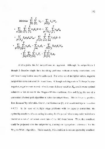
192

N TMinimize X) ^

/=1 i=i j€{I^]

T k T* E E E (c,djk-[) * E E t*pAee{£} k=l i=l g^{GJ p=i

T k

- E E E EM#-0/e{FJ ;e{Z) *=i i=i

T r

^e{G^}p=i p=i fG{F.}

J T NT^E.J^ EW - EEP,y^,j=\f^{Fj)i = l /=h = l

At this point, the J+1 subproblems are apparent. Although the subproblems 1

though J describe single item lot sizing problems without capacity constraints, one

additional complication must be addressed. For some set of multiplier values, negative

subproblem costs can result for .some items. Although ordering costs will always be non-

negative, negative costs associated with some delivery variables could create optimal

solutions which do not fit the Wagner-Whitin conditions, thus nullifying the u.se of a

convenient shortest path algorithm to solve the subproblems. This is the same problem

first discu-ssed by Afentakis, Gavish, and Karmarkar [2], and mentioned again in .section

4.4. 2.3. In the case of multiple stage problems with no capacity constraints, the

optimality condition of zero ending inventory for the period prior to any order period was

treated as a .set of redundant constraints of the full formulation. Thus, that condition

could be projected onto the subproblems, creating an appropriate environment for the

Wagner-Whitin algorithm. Unfortunately, this condition is not an optimality condition

193

for the formulation of section 7.2.2, due to the introduction of capacity constraints.

Nonetheless, we can show that Wagner-Whitin properties may be enforced on the

subproblems, even when they do not necessarily describe at least one optimal solution to

the capacitated multiple stage problem. First, consider the original problem, as formulated

in section 7.2.2. We will name this problem (P), and assume that (P) has non-negative

holding and ordering costs. Next, create problem (P*) from problem (P), by dualizing the

capacity constraints. (P*) describes a multiple stage problem without capacity constraints,

with the same ordering and holding costs associated with problem (P), and non-negative

production costs resulting from the non-negative multipliers of the relaxed constraints.

(The relaxation of the capacity constraints also introduces a negative constant into the

objective function.) As a relaxation, the optimal solution to (P*) will be a lower bound

on the optimal solution to (P). Next, create problem (P") from problem (P*), by relaxing

the family/item ordering constraints. Problem (P*’) describes a problem without joint cost

relationships, in which each item has a non-negative ordering costs resulting from the

multipliers associated with the relaxed family/item ordering constraints, in addition to the

positive holding and production costs of (P'). The optimal solution to (P**) is a lower

bound on the optimal solution to (P*), thus it is a lower bound on the optimal solution to

(P). There also exists at an optimal solution to (P**) which satisfies the Wagner-Whitin

conditions. Thus, to find a lower bound on this optimal solution, we can relax the

parent/child relationships, impose the Wagner- Whitin conditions on the resulting

subproblems, and solve these problems with a shortest path algorithm (as described in

Chapter 4). This lower bound on (P**) is a lower bound on (P), and is the equivalent of

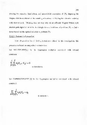
194

relaxing the capacity, family/item, and parent/child constraints of (P), imposing the

Wagner-Whitin conditions on the resulting relaxation, and finding the relaxation solution

with shortest path. Utilizing this, we may rely on an efficient Wagner-Whitin style

shortest path algorithm to solve the J single item subproblems of problem (P), to find a

lower bound on the optimal solution to problem (P).

7.3. 2.2 Statement of procedure

Like all previous bound finding techniques utilized in this investigation, this

procedure is ba.sed on subgradient optimization:

Let MULTIPLIER"(i,j) be the Lagrangian multiplier associated with relaxed

constraint

i T

r*U-rat Iteration n.

Let CAPMULTIPLIER"(i,f) be the Lagrangian multiplier associated with relaxed

constraint

T

,p,,E ^<iit

at Iteration n.

195

Let ORDMULTIPLIER"(i,j,f) be the Lagrangian multiplier associated with relaxed

constraint Yjj - Wj,. < 0 at iteration n.

Let ORDER"(i,j) be the "revised" cost of ordering at least one itemj

in period i,


Let HOLD"(i,j,k) be the "revised" cost of ordering demand lot k in period i, and holding

it in inventory until consumption in period k. This may be interpreted as a production

and holding cost, for it does not include ORDER"(i,j).

Let CONSTANT and CAPCONSTANT be two scalars, 0 < CONSTANT < 2 and 0 <

CAPCONSTANT < 2.

Let n = 0.

N TLet CAP_COST" = EE P.y^.7

/=li=l


Let FAMILY_COST" be the total cost of subproblem J+1.

J

Let TOTALCOST" = TC’'{j) + FAMILYjCOST'' - CAP_COST"

Let SLACK"(i,j) =

196

i T

E E Vr=lk=r

tor I = 1, T; allj

in {Z}.

Let ORDSLACK"(i,j,f) = - W.^ for i = 1, T andj= 1, J.

Let CAPSLACK"(i,0 =

T

E “^if

^^ fori=l,...,Tandf=l,...,N.


a. Let MULTIPLIER"(i,j) = 0 for all i,j.

b. Let CAPMULTlPLlER"(i,f) = 0 for all i,f.

b. Let ORDMULTIPLIER“(i,j,f) = Sjf / rp where r, is the number of items in {IJ,

for all i,j,f.

c. Let ORDER°(i,j) =

EMFj)

V'/

for i = 1, T andj= 1, J.

d. Let HOLD”(iJ,k) = Cjd^j(k - i) for all k, j, and i = 1, k.

197

e. Let LOWERBOUND = 0.


Step 2: Solve suhprohlems.


single level demand requirements for any item g are the demand lots d|g (i=l,...,T). The


ORDER"(i,g) and revised demand lot productiondiolding costs HOLDi^j^, for i = 1, ..., k

and k = 1, ..., T.


c. Calculate ORDSLACK", based on the subproblem solutions.

d. Calculate CAPSLACK", based on the subproblem solutions.

e. Calculate FAM1LY_C0ST".

f. Calculate CAP_COST".

g. Calculate TOTALCOST".

Step 3: Update L(wer Bound.

If LOWERBOUND < TOTALCOST", then LOWERBOUND = TOTALCOST".


a. Let MULTlPLIER""'(i,j) = MULTIPLlER"(i,j) +

CONSTANT * (UPPERBOUND - TOTALCOST'')

N

* SLACK ''{ij)

E E iSLACK''{tSfge{Z} t=\

for all i=l T; allj

in {Z}.

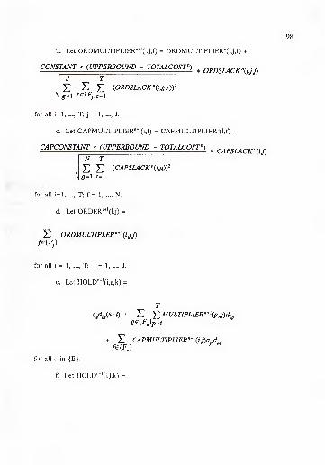
198

b. Let ORDMULTIPLlER''^‘(iJ,f) = ORDMULTlPLlER"(iJ,f) +

CONSTANT * iUPPERBOUND - TOTALCOST'')* ORDSLACK^ij^

J T

E 53 E {ORDSLACK’'it^,r)f

g=l re{F^]t^i

for all i=l, T; j= 1, J.

c. Let CAPMULTIPLIER""'(i,f) = CAPMULTIPLIER"(i,0 +

CAPCONSTANT * (UPPERBOUND - TOTALCOST")* CAPSLACK \if}

N T

Y: E (CAPSLACK'‘(t^)f

g=l t=l

for all 1=1, T; f = 1, •••, N.

d. Let ORDER"^'(i,j) =

E ORDMULTIPLER’'*\ijJ)MFj]

for all i = 1, T; j= 1, J.

e. Let HOLD"^*(i,e,k) =

Tc,djk-i) + E E

S^{Fe^p=i

+ E CAPMULTIPLIER'^*\i/)aJ,^fe{FJ

^

for all e in {E}.

f. Let HOLD""'(i,j,k) =

199

TCjd^ik-i) + E Y^MULTIPLIER''*^(pSdt.

g^{Fj}p=i

T- MULTPLIER''*^(pj)d^j+ E CAPMULTIPLIER''*\i/)a/^^

p=i f^{Fj)

for allj

in {Z}.

g. If LOWERBOUND has not improved in the last three iterations, then

CONSTANT = CONSTANT / 1.1 and CAPCONSTANT = CAPCONSTANT / 1.1.

e. Let n = n + 1. Go to Step 1.


LOWERBOUND is a lower bound on the total cost of an optimal solution. Stop.

7.3. 2.3 Computational Results

Tables 26, 27, and 30 display the bounds found to the supply chain and bottle

racking experiments of Chapter 6. The bounds ranged from within 3.8% to within

16.52% of a heuristic’s solution, averaging a distance of 10.9% across all experiments of

Chapter 7. In the case of each bound, the initial value of CONSTANT was 0.00001 and

the initial value of CAPCONSTANT was 0.01. The procedure outlined in the previous

section was run for 2,000 iterations in the ca.se of each bound. A refinement of this

procedure was also incorporated after early experimentation. The values if q^f, the amount

of re.source f available in period i, were replaced with the valuesq*jf, where;

T

q\^ = MINIMUM{ q.^ E E ^

200

This reduces the total amount of a limited resource available in a given period to

the maximum amount that could be consumed in a feasible solution, given that the

amount is smaller than the total amount available. The effect is a "tightening" of some

capacity constraints, particularly those in later planning periods, without loss of generality.

7.4 Concluding Remarks

Lagrangian relaxation with subgradient optimization has demonstrated its utility

when seeking lower bounds on the optimal .solutions to multiple stage production planning

problems complicated by joint costs and (or) capacity constraints. As was the case with

the bounds found in Chapter 4, the.se results and their subsequent incorporation into the

heuristic analysis of Chapters 5 and 6 repre.sents some of the most ambitious efforts in

the literature. Only a few investigations reviewed in the literature, such as Roundy [78],

provide optimal solutions or lower bounds as benchmarks for evaluating planning

heuristics with Joint costs, but no capacity constraints. One interesting feature of the joint

cost technique outlined in section 7.3. 1.2 is the observation that resulting lower bounds

contained approximately the same proportion of optimal solutions as the lower bounds on

experiments of the same number of items, but no joint costs. This is intriguing in that

more constraints must be dualized in the case of joint costs than in the non-joint cost

relaxation of section 4. 4.2.6. While the bounds found for the joint cost experiments with

capacity constraints were considerably looser, they did provide important benchmarks

usually unavailable in the literature.

CHAPTER 8

CONCLUSIONS

The results of Chapters 3, 5 and 6 demonstrate that the Non-sequential Part Period

Algorithm (NIPPA) is an effective and versatile heuristic technique for multiple stage

production planning. Six other heuristics were incorporated into the evaluation of NIPPA,

none of which exhibited superior average cost performance. NIPPA’s solutions to the

Stage Two experiments of Chapter 3 were, on average, within 1% of a lower bound on

the optimal solutions. While these experiments did not involve joint costs or capacity

constraints, they did include some of the largest product structures and longest planning

horizons examined in the literature. When component commonality was introduced into

the experiments of Chapter 5, NIPPA’s average cost performance was within 1% to 1.2%

of a lower bound on the optimal solution.

The scope of the experiments in Chapters 3 and 5, in terms of the variety of

"improved" heuristics incorporated into the comparative analysis, is the broadest of any

currently available in the literature. In addition to establishing the merits of NIPPA,

insight can be gained into the relative strengths and weaknes.ses of different approaches

to multiple stage planning problems. While multiple pass, iterative procedures such as

NIPPA and Graves’ algorithm required more computational effort than single pa.ss

procedures, they consistently provided superior solutions. When analysis of variance was

conducted for each heuristic, to a.ssess the impact of various experimental factors on the

201

202

ranks of that heuristic’s relative cost ratios, further evidence of the advantages of multiple

pass algorithms came to light. Using a level of significance of .001, the only significant

factor in NIPPA’s ANOVA results was standard deviation of the end item demand

pattern. In contrast, the number of items and the number of levels in the product

structure were significant in the ANOVA results of all single pass algorithms studied in

Chapter 3.

The experiments of Chapter 3 al.so highlighted an interesting issue in multiple

stage experiment design. The researcher’s choice of holding and ordering costs for an

experiment is not a casual one. First, careful attention must he paid to the relative

weights of holding costs, ordering costs, and average demand, or experiments may be

inadvertently created which are easier, if not nearly trivial, to solve. This investigation

developed and utilized the Average Order Cycle (AOC) as a measure of problem

complexity with respect to these parameters. As an alternative. Sum, Png, and Yang [87]

have developed the "batching index", in which any solution that involves too many

(nearly lot-for-lot) or too few order periods indicates an experiment that should be

dropped from the results. However, neither the batching index nor the AOC will reveal

another biasing factor in multiple stage experiment design. Additional experimentation

in Chapter 3 revealed that the relative performances of the single pa.ss heuristics could be

altered dramatically, simply by making the holding and ordering costs of an item some

multiplicative function of the respective costs of its children (for example, .see Veral and

Laforge [90] or Coleman and McKnew [26]), versus choosing both these costs at random

from some uniform distribution (such as in Blackburn and Millen [20] or Afentakis,

203

Gavish and Karmarkar [2]). Therefore, any conclusions concerning the relative

performance of multiple stage planning heuristics should be made with careful

consideration to the nature of the holding and ordering costs used in the evaluation.

The lower bounds on the optimal solutions used as benchmarks for heuristic

performance in Chapters 3, 5 and 6 represent some of the most ambitious in the literature.

Many multiple stage heuristic studies (Bookbinder and Koch [22], Coleman and McKnew

[26], or Sum, Png, and Yang [87], for example) evaluate heuristics relative to other

heuristics included in the study, typically using the cost of the solutions of the best

performing heuristic as a benchmark by which to rate the others. To strengthen the

analysis of this investigation, a method was developed for finding lower bounds on the

optimal solutions to multiple stage planning problems readily considered too large to be

solved with an optimal procedure. The development of this bounding scheme began with

the development of a new formulation for the multiple stage planning problem without

capacity constraints, the new pure binary formulation di.scussed in Chapter 4. Lagrangian

relaxation and subgradient optimization then yielded a bounding scheme that was, on

average, within a maximum of 1% to 1.2% of the optimal solution of the Stage Two,

Chapter 3 and Chapter 5 problems. Both the formulation and this hounding scheme were

extended to multiple stage planning with capacity constraints in Chapter 7, producing

bounds who.se average maximum distance from the optimal solution ranged from 11% for

the supply chain problems to 9.5% for the bottle racking problems of Chapter 6.

The highly generalized joint cost, limited resources problems of Chapter 6

represent multiple stage experiment sets as challenging than any found in the literature

204

surveyed in Chapter 2. The supply chain problems suggest new opportunities in multiple

stage production planning research, addressing the joint manufacturing and distribution

models suggested by Hewlett-Packard [16][66][67]. The bottle racking problem set was

modeled directly from a production facility involving a high degree of component

commonality and multiple limited resources. NIPPA found good quality schedules in

both cases, as confirmed by the lower bounding scheme developed in Chapter 7. It

should be noted that the bounding scheme itself is likely not as tight as the bounding

.schemes developed for use in Chapters 3 and 5. Therefore, a decline in the relative cost

of NIPPA’s solution versus the lower bound in between the experiments of Chapters 3

and 5 and the experiments of Chapter 7 does not necessarily indicate that NIPPA is

finding poorer solutions in the case of Chapter 7. Even if NIPPA’s .solutions were 11%

from the optimal solutions, it is nonetheless developing good quality schedules for a

highly generalized and challenging multiple stage planning environment.

REFERENCE LIST

1. Afentakis, P., and B. Gavish. 1986. Optimal Lot Sizing Algorithm.s for Complex

Product Structures. Operations Research, Vol. 34, 237-24.

2. Afentakis, P., B. Gavish and U. Karmarkar. 1984. Computationally Efficient

Solutions to the Lot Sizing Problem in Multistage Assembly Systems.

Management Science, Vol. 30, 222-239.

3. American Production and Inventory Control Society (APICS). 1974. State of the

Art Survey: A Preliminary Analysis. Production and Inventory Management, Vol.

15, 1-11.

4. Aras, D.A. and L.A. Swanson. 1982. A Lot Sizing and Sequencing Algorithm

for Dynamic Demands Upon a Single Facility. Journal of Operations

Management, Vol. 2, 177-185.

5. Bahl, H.C. 1983. Column Generation Based Heuristic for Multi-item Scheduling.

AIIE Transactions, Vol. 15, 136-141.

6. Bahl, H.C. and L.P. Ritzman. 1984. A Cyclical Scheduling Heuristic for Lot

Sizing with Capacity Constraints. Journal of International Production Research,

Vol. 3, 67-77.

7. Bahl, H.C, L.P. Ritzman and J.N.D. Gupta. 1987. Determining Lot Sizes and

Resource Requirements: A Review. Operations Research, Vol. 35, 329-345.

8. Baker, K.R. 1989. Lot Sizing Procedures and a Standard Data Set: AReconciliation of the Literature. Journal of Manufacturing Operations


9. Benton, S.S. and R. Srivastava. 1985. Product Structure Complexity and

Multilevel Lot Sizing Using Alternative Costing Policies. Decision Sciences, Vol.

16, 357-369.

10. Berry, W.L. 1972. Lot Sizing Procedures for Requirements Planning Systems:

A Framework for Analysis. Production and Inventory Management, 2nd Quarter,

19-34.

205

206

11. Berry, W.L., T.E. Vollman and D.C. Whybark. 1979. Master Production

Scheduling: Principles and Practice. American Production and Inventory Control

Society, Milwaukee.

12. Biggs, J.A. 1979. Heuristic Lot Sizing and Sequencing Rules in a Multistage

Production and Inventory System. Decision Sciences, Vol. 10, 96-115.

13. Biggs, J.R. 1985. Priority Rules for Shop Floor Control in a Material

Requirements Planning System Under Various Levels of Capacity. International

Journal of Production Research, Vol. 23, p. 33-46.

14. Biggs, J.A., S.H. Goodman and S.T. Hardy. 1977. Lot Sizing Rules in a

Hierarchical Multi-stage Inventory System. Production and Inventory


15. Biggs, J.R. , C.K. Hahn, and P.A. Pinto. 1980. Performance of Lot-Sizing Rules

in an MRP System with Different Operating Conditions. Academy ofManagement

Review, Vol. 5, 89-96.

16. Billington, C. 1994. Strategic Supply Chain Management. ORIMS Today, ApxW,

20-27.

17. Billington, P.J., J.O. McClain and L.J. Thomas. 1983. Mathematical

Programming Approaches to Capacity Constrained MRP Systems: Review,

Formulation, and Problem Reduction. Management Science, Vol. 29, 1126-1141.

18. Bitran, G.R. and H.H. Yanasse. 1982. Computational Complexity of the

Capacitated Lot Size Problem. Management Science, Vol. 28, 1174-1186.

19. Blackburn, J.D. and R.A. Millen. 1980. Heuristic U')t-Sizing Performance in a

Rolling Schedule Environment. Decision Sciences, Vol. 11, 691-701.

20. Blackburn, J.D. and R.A. Millen. 1982. Improved Fleuristics for Multistage

Requirements Planning Systems. Management Science, Vol. 28, 44-56.

21. Blackburn, J.D. and R.A. Millen. 1985. An Evaluation of Heuristic Performance

in Multi-Stage Lot-Sizing Systems. InternationalJournal ofProduction Research,

Vol. 23, 857-866.

22. Bookbinder, J.H. and L.A. Koch. 1990. Production Planning for Mixed

Assembly/Arborescent Systems. Journal ofOperations Management, Vol. 9, 7-23.

23. Box, G.E.P. and D.R. Cox. 1964. An Analysis of Transformations. Journal of

the Royal Statistical Society, Volume B26, 21 1-243.

207

24. Chung, C.S. and H.M. Mercan. 1994. Heuristic Procedure for a Multiproduct

Dynamic Lot-Sizing Problem with Coordinated Replenishments. Naval Research

Logistics, Vol. 41, p. 273-286.

25. Coleman, B.J., and M.A. McKnew. 1990. A Technique for Order Placement and

Sizing. Journal of Purchasing and Materials Management, Vol. 26, 32-40.

26. Coleman, B.J., and M.A. McKnew. 1991. An Improved Heuristic for Multilevel

Lot Sizing in Material Requirements Planning. Decision Sciences, Vol. 22, 136-

156.

27. Collier, D.A. 1980. A Comparison of MRP Lot Sizing Methods Considering

Capacity Change Cost. Journal of Operations Management, Vol. 1, 23-29.

28. Collier, D.A. 1982. Aggregate Safety Stock Levels and Component Part

Commonality. Management Science, Vol. 28, 1296-1303.

29. Crowston, W.B., and M.H. Wagner. 1973. Dynamic Lot Size Models for

Multistage A.ssembly Systems. Management Science, Vol. 20, 14-21.

30. Crowston, W.B, M.H. Wagner, and A. Henshaw. 1972. Comparison of Exact and

Heuristic Routines for Lot-Size Determination in Multi-Stage A.ssembly Systems.

AIIE Transactions, Vol. 4, 313-317.

31. Crow.ston, W.B., M.H. Wagner and J. Williams. 1973. Economic Lot Size

Determination in Multistage A.ssembly Systems. Management Science, Vol. 19,

517-526.

32. Davis, T. 1993. Effective Supply Chain Management. Sloan Management

Review, Vol. 34, 35-46.

33. Dixon, P.S. and E.A. Silver. 1981. A Heuristic Solution Procedure for the Multi-

item, Single-level, Limited Capacity Lot Sizing Problem. Journal of Operations


34. Dogramci, A., J.C. Panayiotopoulos and N.G. Adam. 1981. The Dynamic Lot-

Sizing Problem for Multiple Items Under Limited Capacity. AIIE Transactions,

Vol. 13, 294-326.

35. Duenyas, 1. and W.J. Hopp. 1990. CONWIP Assembly with Deterministic and

Random Outages. HE Transactions, Vol. 24, 97-109.

36. Dzielinski, B., C.T. Baker and A.S. Manne. 1963. Simulation Tests of Lot Size

Programming. Management Science, Vol. 9, 229-258.

208

37. Dzielin.ski, B. and P. Gomory. 1965. Optimal Programming of Lot Sizes,

Inventories and Labor Allocations. Management Science, Vol. 11, 874-890.

38. Eisenhut, P.S. 1975. A Dynamic Lot Sizing Algorithm with Capacity

Constraints. AIIE Transactions, Vol. 7, 170-176.

39. Elmaghraby, S.E. 1978. The Economic Lot Scheduling Problem (ELSP):

Review and Extension. Management Science, Vol. 24, 587-598.

40. Erenguc, S.S. 1988. Multiproduct Dynamic Lot-Sizing Model with Coordinated

Replenishments. Naval Research Logistics, Vol. 35, 1-22.

41. Erenguc, S.S. and H.M. Mercan. 1990. A Multifamily Dynamic Uit-Sizing

Model with Coordinated Replenishments. Naval Research Logistics, Vol. 37, p.

539-558.

42. Fisher, M.L. 1981. The Lagrangian Relaxation Method for Solving Integer

Programming Problems. Management Science, Vol. 27, 1-18.

43. Florian, M., J.K. Lenstra, and A.H.G. Rinnooy Kan. 1980. Deterministic

Production Planning: Algorithms and Complexity. Management Science, Vol. 26,

12-20 .

44. Freeland, J.R. and J.L. Colley. 1982. A Simple Heuristic Method for Lot-Sizing

in a Time Phased Reorder System. Production and Inventory Management, 1st

Quarter, 15-22.

45. Fry, T.D., J.F. Cox and J.H. Blackstone. 1992. An Analysis and Discussion of

the Optimized Production Technology Software and Its Use. Production and

Operations Management, Vol. 1, 229-242.

46. Gabby, H. 1979. Multi-stage Production Planning. Management Science, Vol.

25, 1138-1148.

47. Gaither, N. 1981. A Near-Optimal Lot-Sizing Model for Material Requirements

Planning Systems. Production and Inventory Management, 4th Quarter, 75-89.

48. Geoffrion, A.M. 1974. Lagrangean Relaxation for Integer Programming.

Mathematical Programming Study, Vol. 2, 82-1 14.

49. Glover, F. 1989. Tabu Search-Part I. ORSA Journal of Computing, Vo\. \, \90-

206.

209

50. Goldratt, E.M. 1980. Optimized Production Timetable: A Revolutionary

Program for Industry. APICS 23th Annual International Conference Proceedings,

Los Angeles.

51. Goldratt, E.M. 1982. 100% Data Accuracy- Need or Myth? APICS 25th Annual

International Conference Proceedings, Chicago.

52. Graves, S.C. 1981. Multi-Stage Lot-Sizing: An Iterative Procedure. In Multi-

Level Produclionlinventory Control Systems: Theory and Practice, L.B. Schwarz

(ed.). North-Holland, Amsterdam.

53. Haehling Von Lanzenhauer, C. 1970. Production and Employment Scheduling

in Multi-Stage Production Systems. Naval Research Logistics Quarterly, Vol. 17,

193-198.

54. Harl, J.E. and L.P. Ritzman. 1985. An Algorithm to Smooth Near-Term Capacity

Requirements Generated by MRP Systems. Journal of Operations Management,

Vol. 5, 309-326.

55. Harris, F.W. 1915. Operations and Cost. \n Factory Management Series. A.W.

Shaw Co., Chicago.

56. Ho, C. 1993. Evaluating Lot-Sizing Performance in Multi-level MRP Systems:

A Comparative Analysis of Multiple Performance Measures. International

Journal of Operations and Production Management, Vol. 13, p. 52-79.

57. lyogun, P. and D. Atkins. 1993. A Lower Bound and an Efficient Heuristic for

Multistage Multiproduct Distribution Systems. Management Science, Vol. 39,

204-217.

58. Jackson, P.L., W.L. Maxwell and J.A. Muckstadt. 1988. Determining Optimal

Reorder Intervals in Capacitated Production-Distribution Systems. Management

Science, Vol. 34, 938-958.

59. Kaimann, R.A. 1969. EOQ vs. Dynamic Programming - Which One to Use for

Inventory Ordering? Production and Inventory Management, Vol. 10, 66-74.

60. Kao, E.P.C. 1979. A Multi-Product Dynamic Lot-Size Model with Individual and

Joint Set-up Costs. Operations Research, Vol. 27, 279-289.

61. Kuehl, R.O. 1994. Statistical Principles of Research Design and Analysis.

Duxbury Pre.ss, Belmont.

210

62. Laforge, R.L. 1982. MRP and the Part Period Algorithm. 7o«</7i<7/ r;/P»rc/ia5m^

and Materials Management, Vol. 18, 21-26.

63. Lambrecht, M.R. and Vandervecken, H. 1979. Heuristic Procedures for the

Single Operation Multi-item Loading Problem. AUE Transactions, Vol. 15, 319-

326.

64. Lasdon, L.S. and R.C. Terjung. 1971. An Efficient Algorithm for Multi-item

Scheduling Problems. Operations Research, Vol. 19, 946-969.

65. Lee, H.L. and C. Billington. 1992. Managing Supply Chain Inventory: Pitfalls

and Opportunities. Sloan Management Review, Vol. 33, 65-73.

66. Lee, H.L. and C. Billington. 1993. Material Management in Decentralized

Supply Chains. Operations Research, Vol. 41, 835-847.

67. Lee, H.L., C. Billington and B. Carter. 1993. Hewlett-Packard Gains Control of

Inventory and Service Through Design for Localization. Interfaces, Vol. 23, p.

1 - 11 .

68. Lrwe, S.F. 1972. A Facilities in Series Inventory Model with Nested Schedules.


69. Maes, J. and L.N. Wassenhove. 1986. Multi-item Single Level Capacitated

Dynamic Lot Sizing Heuristics: A Computational Comparison (Part 1: Static

Case). AIIE Transactions, June 1986, 114-123.

70. Manne, A.S. 1958. Programming of Economic Lot Sizes. Management Science,

Vol. 4, 115-135.

71. Maxwell, W.L. and J.A. Muckstadt. 1985. Establishing Consistent and Realistic

Reorder Inteiwals in Production-Distribution Systems. Operations Research, Vol.

33, 1316-1341.

72. McClain, J.O., et al. 1982. A Note on MRP Lot Sizing. Management Science,

Vol. 28, 582-584.

73. McKnew, M.A., Saydam, C., and Coleman, B.J. 1991. An Efficient Zero-One

Formulation of the Multilevel Lot-Sizing Problem. Decision Sciences, Vol. 22,

280-295.

74. Newson, E.F. and P.D. Kleindorfer. 1975. A Lower Bounding Structure for Lot

Size Scheduling Problems. Operations Research, Vol. 23, 299-311.

211

75. Rajagopalan, S. 1992. A Note on "An efficient zero-one formulation of the

multilevel lot-sizing problem." Decision Sciences, Vol. 23, 1023-1025.

76. Raturi, A.S. and A.V. Hill. 1988. An Experimental Analysis of Capacity

Sensitive Setup Parameters for MRP Lot Sizing. Decision Sciences, Vol. 19, 782-

800.

77. Roundy, R.O. 1986. 98% Efficient, Effective Lot Sizing for Multi-Product,

Multi-Stage Production/Inventory Systems. Mathematics ofOperations Research,

Vol. 11, 699-727.

78. Roundy, R.O. 1993. Efficient, Effective Lot Sizing for Multistage Production

Systems. Operations Research, Vol. 41, 371-385.

79. Schussel, G. 1968. Job-Shop Release Sizes. Manaf’ement Science, Vol. 14,

B449-B472.

80. Schwarz, L.B. and L. Schrage. 1975. Optimal and System Myopic Policies for

Multi-Echelon Production/Inventory A.ssembly Systems. Management Science,

Vol. 21, 1285-1294.

81. Silver, E.A. and H.C. Meal. 1973. A Heuristic for Scheduling Lot Size

Quantities for the Case of a Deterministic Time-Varying Demand Rate and

Discrete Opportunities for Replenishment. Production and Inventory Management,

Vol. 14, 64-74.

82. Spearman, M.L., D.L. Woodruff, and W.J. Hopp. 1990. CONWIP: A Pull

Alternative to Kanban. International Journal of Production Research, Vol. 28,

879-894.

83. Spearman, M.L. and M.A. Zazanis. 1992. Push and Pull Production Systems:

Issues and Comparisons. Operations Research, Vol. 40, 521-532.

84. Steinberg, E. and H.A. Napier. 1980. An Optimal Multi-Level Sizing for

Requirements Planning Systems. Management Science, Vol. 26, 1258-1271.

85. Steinberg, E. and H.A. Napier. 1982. On "A Note on MRP Lot Sizing".


86. Sum, C.C. and A.V. Hill. 1993. A New Framework for Manufacturing Planning

and Control Systems. Decision Sciences, Vol. 24, 739-760.

87. Sum, C.C., D.O.S. Png and K.K. Yang. 1993. Effects of Product Structure

Complexity on Multi-level Lot Sizing. Decision Sciences, Vol. 24, 1 135-1156.

212

88. Tersine, R.J. 1988. Principles of Inventory and Materials Manaf'ement. North

Holland, Amsterdam.

89. Veinott, A.F., Jr. 1969. Minimum Concave-Cost Solution of Leontief

Substitution Models of Multifacility Inventory Systems. Operations Research,

Vol. 7, 262-290.

90. Veral, E. and R.L. LaForge. 1985. The Performance of a Simple Incremental Lot

Sizing Rule in a Multi-Level Inventory Environment. Decision Sciences, Vol. 16,

57-72.

91. Vollman, T.E, W.L. Berry and D.C. Whybark. 1992. Manufacturing Planning

and Control Systems. Richard D. Irwin, Inc., Boston.

92. Wagner, M.H., and T.M. Whitin. 1958. Dynamic Version of the Economic Lot

Sizing Model. Management Science, Vol. 5, 89-96.

93. Williams, J.F. 1981. Heuristic Techniques for Simultaneous Scheduling of

Production and Distribution in Multi-Echelon Structures: Theory and Empirical

Comparisons. Management Science, Vol. 27, 336-352.

94. Zahorik, A., L.J. Thomas and W.B. Trigeiro. Network Programming Models for

Production Scheduling in Multi-stage, Multi-item Capacitated Systems.


95. Zangwill, W.I. 1966. A Deterministic Multiproduct Multifacility Production and

Inventory Model. Operations Research, Vol. 4, 486-507.

96. Zangwill, W.I. 1969. A Backlogging Model and a Multi-Echelon Model of a

Dynamic Economic Lc)t Size Production System - A Network Approach.


BIOGRAPHICAL SKETCH

Natalie Simpson received a Bachelor of Fine Arts from North Carolina School of

the Arts and a Master of Business Administration from the University of Florida. She has

received recognition for both scholarship and teaching, including a Grinter Fellowship

from the Graduate School of the University of Florida, and a Graduate Student Teaching

Award. Natalie is a member of the Decision Sciences Institute and Alpha lota Delta.

213

I certify that I have read this study and that in my opinion it conforms to

acceptable standards of scholarly presentation and is fully adequate, in scope and quality,



as a dissertation for the degree of Doctor of Philosophy.

Harold P. Benson

Professor of Decision and Information

Sciences




Chung Yee Lee

Professor of Industrial and Systems

Engineering




Antal Majthay

Associate Professor of Decision and

Information Sciences




Patrick A. Thompson

Assistant Professor of Decision and

Information Sciences

This dissertation was submitted to the Graduate Faculty of the College of Business

Administration and to the Graduate School and was accepted as partial fulfillment of the

requirements for the degree of Doctor of Philosophy.

August 1994

Dean, Graduate School

METHODS STAGE MANUFACTURING

Documents

Transcript of METHODS STAGE MANUFACTURING