Methods of Generating Synthetic Acoustic Logs from ... · Methods of Generating Synthetic Acoustic...

Methods of Generating Synthetic Acoustic Logsfrom Resistivity Logs for Gas-Hydrate-BearingSediments

By

Myung W. Lee

U.S. Geological Survey Bulletin 2170

U.S. Department of the InteriorU.S. Geological Survey

U.S. Department of the Interior

Bruce Babbitt, Secretary

U.S. Geological Survey

Charles G. Groat, Director

This publication is only available on line at:

http://greenwood.cr.usgs.gov/pub/bulletins/b2170/index.html

Any use of trade, product, or firm names in this publicationis for descriptive purposes only anddoes not imply endorsement by the U.S. Government

Published in the Central Region, Denver, ColoradoManuscript approved for publication July 19, 1999Graphics by Norma J. MaesPhotocomposition by Norma J. MaesEdited by Lorna Carter

III

Contents

Abstract ................................................................................................................................................. 1Introduction........................................................................................................................................... 1Acknowledgments ............................................................................................................................... 1Theoretical Relationship ..................................................................................................................... 1Logs and Parameters........................................................................................................................... 3Modified Time Average Equations .................................................................................................... 3Predicting Velocity from Resistivity .................................................................................................. 3

Without Gas Hydrate Concentration........................................................................................ 3With Gas Hydrate Concentration.............................................................................................. 4

Discussion ............................................................................................................................................. 4Conclusions........................................................................................................................................... 9References Cited.................................................................................................................................. 10

Figures

1–8. Graphs showing:

1. Electrical resistivity measured at Mallik 2L-38 gas hydrate research well with respect to density porosity for depth range 897 m to 1,109 m ......... 4

2. Comparison of

P

-wave velocities computed from weighted equation with

W

=1.44 and modified time average equations where

α

=1.3 and

β

=1.68 ........................................................................................ 53. Prediction of acoustic values from resistivity log at Mallik 2L-38 well

using least squares method.................................................................................... 64. Prediction of acoustic values from resistivity log at Mallik 2L-38 well

using modified time average equations without gas hydrate concentration. 75. Acoustic values predicted from resistivity log at Mallik 2L-38 well using

modified time average equations with gas hydrate concentration ................. 86. Comparison of acoustic values from resistivity log at Mallik 2L-38 well

using WE and MTAE2 with gas hydrate concentration...................................... 97. True (measured) acoustic values versus predicted acoustic values using

LSM, MTAE1, and MTAE2 ........................................................................................ 108. Theoretical unconsolidation constants with respect to porosity and

weights of WE ........................................................................................................... 10

1

Methods of Generating Synthetic Acoustic Logs from Resistivity Logs for Gas-Hydrate-Bearing Sediments

By

Myung W. Lee

Abstract

Methods of predicting acoustic logs from resistivity logs for hydrate-bearing sediments are presented. Modified time average equations derived from the weighted equation provide a means of relating the velocity of the sediment to the resistivity of the sediment. These methods can be used to transform resistiv-ity logs into acoustic logs with or without using the gas hydrate concentration in the pore space. All the parameters except the unconsolidation constants, necessary for the prediction of acous-tic log from resistivity log, can be estimated from a cross plot of resistivity versus porosity values. Unconsolidation constants in equations may be assumed without rendering significant errors in the prediction. These methods were applied to the acoustic and resistivity logs acquired at the Mallik 2L-38 gas hydrate research well drilled at the Mackenzie Delta, northern Canada. The results indicate that the proposed method is simple and accurate.

Introduction

One of the problems in the seismic study of hydrate-bearing sediments is the lack of available acoustic logs. Older wells usu-ally have resistivity logs, but not acoustic logs. Even in cases where acoustic logs exist, most of the time the acoustic values in the hydrate-bearing sediment intervals are useless because of well bore problems associated with the dissociation of gas hydrate. Therefore being able to predict acoustic values from resistivity logs or to transform pseudo-velocity logs from resis-tivity logs is useful in gas hydrate research.

Many methods for predicting acoustic logs from resistivity logs have been proposed (Faust, 1951; Kim, 1964; Rudman and others, 1975; Brito Dos Santos and others, 1988; Worthington, 1991). Most of these methods utilize the time average equation of Wyllie and others (1958) and Archie’s law (Archie, 1942). The difference among the methods is the way to link the time average equation to Archie’s law.

Faust (1951) developed an empirical formula to relate velocities to depth and age of the rocks. Using Archie’s law with his empirical formula, Faust developed a relationship between the velocity and apparent resistivity, which is thought to be applicable primarily to permeable formations.

Kim (1964) demonstrated that a mathematical relation could be developed between apparent resistivity and travel time (acoustic value). The mathematical formula indicates that three parameters, related to the physical properties of the sediments, are sufficient to predict acoustic values from resistivity values. Instead of using physically significant parameters to derive the constants, Kim solved nonlinear simultaneous equations using

three different resistivity-acoustic values. In essence, this is sim-ilar to the least squares method of nonlinear curve fitting. Because Kim selected good and consistent resistivity-acoustic values, it can be said that this method is based on the weighted least squares method.

Rudman and others (1975) slightly modified Kim’s approach and used the average scale function (a scale function is a predictive function that specifies a corresponding transit time for any resistivity value) to predict acoustic values from resistiv-ity measurements; they suggested the application, with caution. They recommended that the resistivity range recorded be exam-ined and those logs with anomalous values be discarded.

Brito Dos Santos and others (1988) presented a method uti-lizing the resistivity of mud, resistivity of mud-filtrate-contain-ing rock, and resistivity of clay with Bussian’s (1983) equation, which is more general than Archie’s equation for the sediment’s resistivity. In essence, this method provides a better prediction of acoustic values by accounting for the shaly sand effect on the resistivity logs. To account for the clay effect on acoustic logs as well as resistivity logs, Worthington (1991) presented equations containing explicit clay terms in the time average and resistivity equations.

In this report, Archie’s equation for dirty shaly sands and modified time average equations using unconsolidation con-stants are combined to link the resistivity values to the velocities through the common parameter of porosity. The proposed meth-ods implicitly account for the clay effect by using modified matrix velocity (Lee and others, 1996) and Archie’s parameter for dirty sands. These methods were applied to the log data acquired at the Mallik 2L-38 gas hydrate research well with good agreement.

Acknowledgments

Well logs were acquired by Schlumberger Ltd. at the Mallik 2L-38 gas hydrate research well, which was drilled to investigate gas hydrate in a collaborative research project among Japan National Oil Company, Japan Petroleum Exploration Company, Geological Survey of Canada, and U.S. Geological Survey. I thank Tim Collett and Dave Taylor for many helpful comments.

Theoretical Relationship

The simplest equation relating the acoustic value to sedi-ment’s porosity is the time-average equation by Wyllie and oth-ers (1958). This equation works well for consolidated sediments, but it is problematic when applied to unconsolidated sediments. In order to overcome the unconsolidation problem of

2 Methods of Generating Synthetic Acoustic Logs from Resistivity Logs for Gas-Hydrate-Bearing Sediments

the sediments using the time average equation, particularly for the hydrate-bearing sediments, Lee and others (1996) introduced a weighted equation (WE). This WE works well for hydrate-bearing sediments or permafrost samples (Lee and others, 1996; Lee and Collett, 1999). However, predicting velocities from resistivities using WE is not simple, mainly because the velocity from WE equation is a complex function of porosity. Thus, equations similar to the time average equation are useful to for-mulate the relationship between the resistivity of sediments and the transit time of the compessional wave. To account for the unconsolidation of sediments and to relate the porosity to the velocity, WE is approximated in the following way.

WE for non-hydrate-bearing sediments is defined by (Lee and others, 1996):

(1)

where

L

we

is the slowness computed using the weighted equa-tion,

L

wd

is the slowness computed using the Wood equation,

L

ta

is the slowness computed using the time-average equation,

W

is the weight and

φ

is

the porosity of the sediment.The time average equation is defined by

(2)

where

S

f

is the slowness of the pore fluid, and

S

m

is the slowness of the modified matrix, which accounts for the clay content in sediment, as explained in Lee and others (1996).

The first approximation of WE, which is called the modi-fied time average equation 1 (MTAE1), is defined as follows, from equation (1):

(3)

where

α

is assumed to be a constant, whereas in fact it is a func-tion of porosity and physical properties of sediments. The accu-racy of this approximation will be discussed later. Since

W

is positive and

L

wd

is greater than

L

ta

,

α

is always greater than or equal to 1.0 and called the

α

-unconsolidation constant.The second approximation of WE, which is called the mod-

ified time average equation 2 (MTAE2), is defined as follows, using equations (1) and (2):

(4)

where

β

is defined as a constant and called the

β

-unconsolidation constant. As in MTAE1,

β

is always greater than or equal to 1.0. When the sediment pore spaces are occupied by the gas

hydrates, the modified time average equations can be written as (Lee and others, 1996):

Lwe Lta Wφ+ Lwd Lta–( )=

Lta S( f Sm )– φ Sm+=

MTAE1 Lwe Lta 1Wφ L( wd Lta )–

Lta--------------------------------------+ αLta≈=≈

MTAE2 Lwe S( f Sm )–= φ 1 WφW L( wd Sm )–

S f Sm–------------------------------------+– Sm+≈

S( f Sm– )βφ Sm+≈

(5a)

(5b)

where

C

is the gas hydrate concentration and

S

h

is the slowness of the gas hydrates.

The electrical property of sediment can be described by Archie’s formula (Archie, 1942), which is given by

(6)

where

R

t

is the resistivity of the sediments,

R

w

is the resistivity of pore fluid,

C

w

is the fluid saturation, and

a

,

n

, and

m

are Archie’s empirically derived parameters. Usually

a

ranges from 0.55 to 2.26,

n

varies between 1.7 and 2.2 (Pearson and others, 1983), and

m

can have values between 1 and 3 (Labo, 1987). If the gas hydrate in the pore space is considered as part of the matrix, then the water saturation

C

w

is equal to 1 and the poros-ity in equations (1) and (6) can be considered as water-filled (

φ

f

) porosity, which is defined

φ

f

= (1–

C

h

)

φ

, where

C

h

is the gas hydrate concentration.

For clean sands,

a

= 1.0 and

m

=2.0 are proper parameters to use. The deviation of the empirically derived

a

and

m

from those of the clean sands is partly due to the clay content in the sediments in addition to the complex pore geometry. In this report, we assume that the clay in the formation resistivity is manifested in Archie’s parameters

a

and

m

.With 100 percent water saturation or using the water-filled

porosity in the Archie’s equation, the water saturation can be set to 1 for hydrate-bearing sediments. So, defining

Q=

(1/

aR

w

) and substituting the porosity in equation (6) into the modified time average equations, the relationship between the acoustic and resistivity can be written as

(7)

Or

(8)

where

S

´

is defined as a normalized acoustic,

η

1

and

η

2

are

α

’s for MTAE1, and

η

1

=

β

and

η

2

=1 for MTAE2. Equation (8) shows a linear relationship between a normalized acoustic and resistivity in a Log-Log plot. Equation (6) also indicates a linear relationship between porosity and the resistivity in a Log-Log plot. If data quality is good, the slope from equation (8) should be close to that estimated from the resistivity log using equation (6).

Most of the parameters necessary for the use of equation (7) to compute the

P

-wave acoustic values from resistivity log val-ues can be estimated directly from the resistivity versus density data. For 100 percent water saturation (baseline data without gas hydrate concentration), the slope of the Log-Log plot of porosity

MTAE1 α CSh 1 C–( )S f Sm–+[ ]φ αSm+=

MTAE2 β CSh 1 C–( )S f Sm–+[ ]φ Sm+=

φ m– Cnw Rt

aRw---------------

=

Log10S η2Sm–

η1Sw η1Sm–-------------------------------- Log10S′≡

Log10Q

m--------------------–

Log10Rt

m---------------------–=

S Sw S– m( )η1φ η2Sm+ Sw S– m( )η1Q1 m⁄–

Rt1 m⁄– η2Sm+= =

Logs and Parameters 3

and resistivity provides the parameter m, and the intercept at Rt = 1 ohm-m provides the value for Q = 1/(aRw).

Logs and Parameters

Resistivity and acoustic logs were acquired at the Mallik 2L-38 gas hydrate research well at the Mackenzie Delta, northern Canada, in 1998 (Collett and others, 1999). The quality of data is excellent, and porosities derived from the density log were used in this study. Previous studies (Lee and Collett, 1999) estimated some relevant parameters for this study. A WE (weighted equation) with the weight of W= 1.44 and the expo-nent of n = 1 with other parameters such as Sf = 0.667 s/m, Sh = 0.303 s/m, and Sm = 0.2024 s/m was used in the previous study (Lee and Collett, 1999) to estimate gas hydrate concentration from acoustic logs. The slowness of modified matrix (Sm) is cal-culated from Han and others’ relation (1986) using the volume clay content of 30 percent. These parameters were used in this study.

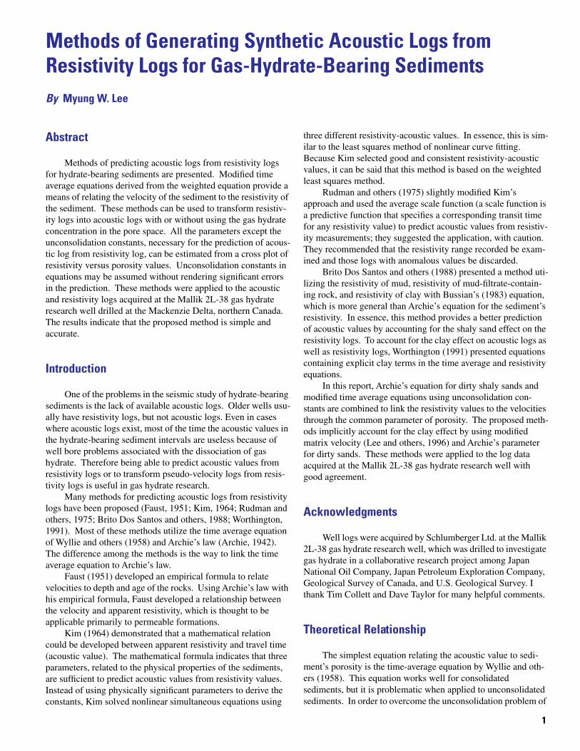
Figure 1 shows a cross plot of Log10 (φ) versus Log10 (Rt) for the depth range of 897 m to 1,109 m. Using the slope of the linear approximation for the non-hydrate-bearing sediment data shown in figure 1, m is estimated as m = 1.95. The intercept of the linear approximation at Rt = 1 ohm-m is about 0.63. Substituting this value into equation (8), it can be shown that Q = 0.406.

Modified Time Average Equations

To examine the behavior of modified time average equa-tions with respect to WE for the velocities of unconsolidated sediments, velocities from WE with W=1.44 and Sm = 0.2024 s/m are compared with those from the modified time average equations. Figure 2 shows the theoretical velocities using WE with those from the modified time average equations. The com-putation of unconsolidation parameters can be done in two ways:

1. Match the observed velocity at a given porosity with the modified time average equations shown in equations (3) and (4).

2. When the parameters for WE are known, the unconsoli-dation parameters can be calculated using W in the definition of unconsolidation parameters. In this example, unconsolidation constants were computed by matching the velocities for the sediment having a porosity of 33 percent, and they are given by α =1.3 and β =1.68. Without unconsolidation correction, the time average equation predicts a velocity of 2.81 km/s for 33 percent sediment porosity with 30 percent clay volume content, while the MTAE2 predicts a veloc-ity of 2.16 km/s. The velocities predicted from WE are very close to those calculated from MTAE; however, the theoretical velocities from MTAE1 are less than those from WE or MTAE2 for porosity less than 33 percent and greater than those from WE and MTAE2 for porosity greater than 33 percent. As is shown later, each equation, MTAE1 or MTAE2, has its own advantage in predicting acoustic velocities from resistivities.

Predicting Velocity from Resistivity

Velocities of hydrate-bearing sediments can be predicted from resistivity logs with or without knowing gas concentrations in the pore space.

Without Gas Hydrate Concentration

The basic equation predicting the acoustic values from the resistivities is equation (7). Because the gas hydrate concentra-tions are not explicitly utilized in the method, the porosity in equation (7) can be considered as the water-filled porosity. One well-known method is fitting acoustic values to resistivity values using the least squares method (Kim, 1964; Rudman and others, 1975). As indicated in equation (7), the acoustic values can be written in the following way:

(9)

where parameters A, B, and D can be estimated by the least squares method. Notice that in applying equation (9), any explicit information such as Archie’s parameters or slowness of the constituents of sediments is not required, but acoustic and resistivity logs should be available for analysis. Originally Kim (1964) proposed a method of obtaining three parameters by solv-ing three nonlinear simultaneous equations from three resistiv-ity-acoustic values. This is similar to the least squares method mentioned here, where all available resistivity-acoustic values are used in the least squares method. Because the selection of three pairs of resistivity-acoustic values is subjective, Kim’s approach can be considered as a weighted least squares method.

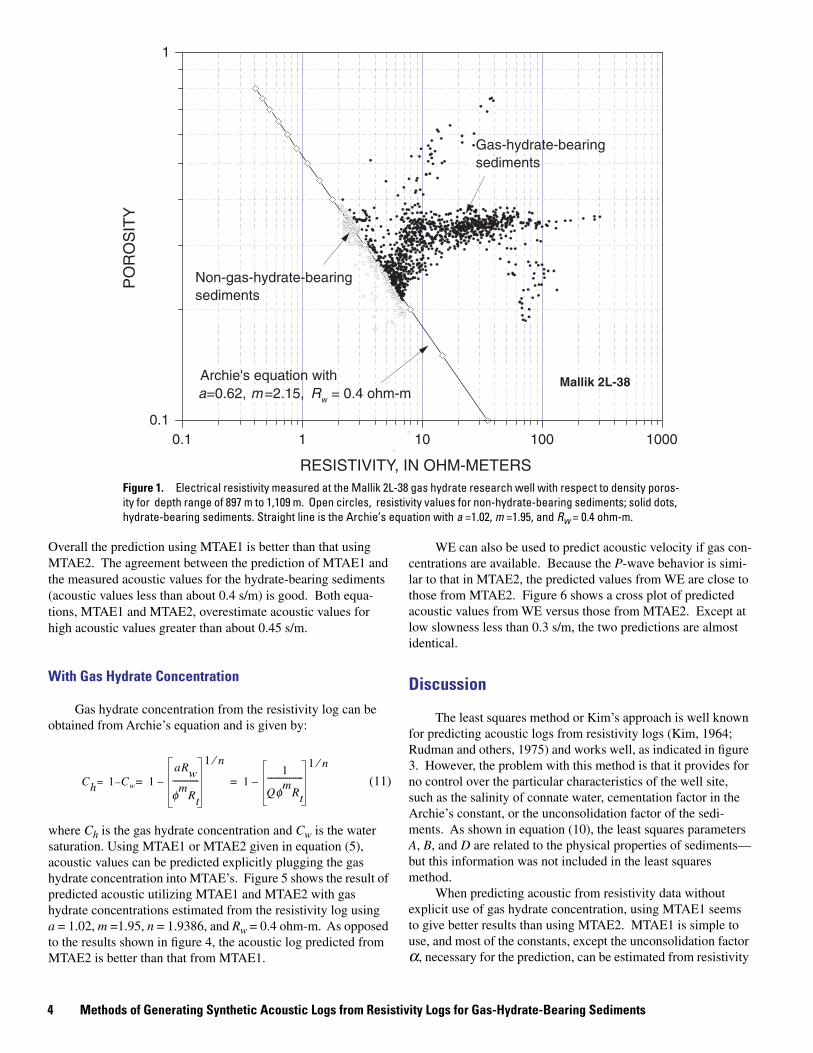
An example of the application of this method is shown in figure 3. Figure 3A shows the least squares fitting curve with acoustic and resistivity data, and figure 3B shows the compari-son of measured versus predicted acoustic values with depth. Because the prediction is done using the least squares method, the difference of the average acoustic values between the mea-sured and predicted is zero.

Another method of predicting acoustic values from resis-tivity logs is to use MTAE1 or MTAE2 with explicit informa-tion about the resistivity log and physical properties of corresponding sediments. The required parameters are m and Q from the resistivity log and slowness (inverse of velocity) of modified matrix and unconsolidation constants for the acoustic properties of sediments. In principle, this method is similar to Kim’s method, whereby the parameters were derived from the physical properties of sediments rather than estimated using least squares method. Kim’s parameters A, B, and D can be identified as

(10)

Figure 4 shows the predicted acoustic values using MTAE1 and MTAE2 with parameters shown in the previous section.

S ARtB

D+=

A Sw S– m( )η1Q1 m⁄–

B 1 m D,⁄–=, η2Sm= =


0.1 1 10 100 10000.1

1

Mallik 2L-38

Gas-hydrate-bearingsediments

Archie's equation witha=0.62, m =2.15, Rw = 0.4 ohm-m

Non-gas-hydrate-bearingsediments

RESISTIVITY, IN OHM-METERS

PO

RO

SIT

Y

Overall the prediction using MTAE1 is better than that using MTAE2. The agreement between the prediction of MTAE1 and the measured acoustic values for the hydrate-bearing sediments (acoustic values less than about 0.4 s/m) is good. Both equa-tions, MTAE1 and MTAE2, overestimate acoustic values for high acoustic values greater than about 0.45 s/m.

With Gas Hydrate Concentration

Gas hydrate concentration from the resistivity log can be obtained from Archie’s equation and is given by:

(11)

where Ch is the gas hydrate concentration and Cw is the water saturation. Using MTAE1 or MTAE2 given in equation (5), acoustic values can be predicted explicitly plugging the gas hydrate concentration into MTAE’s. Figure 5 shows the result of predicted acoustic utilizing MTAE1 and MTAE2 with gas hydrate concentrations estimated from the resistivity log using a = 1.02, m =1.95, n = 1.9386, and Rw = 0.4 ohm-m. As opposed to the results shown in figure 4, the acoustic log predicted from MTAE2 is better than that from MTAE1.

Ch 1= Cw– 1aRw

φmRt

-------------

1 n⁄

–= 11

QφmRt

------------------1 n⁄

–=

WE can also be used to predict acoustic velocity if gas con-centrations are available. Because the P-wave behavior is simi-lar to that in MTAE2, the predicted values from WE are close to those from MTAE2. Figure 6 shows a cross plot of predicted acoustic values from WE versus those from MTAE2. Except at low slowness less than 0.3 s/m, the two predictions are almost identical.

Discussion

The least squares method or Kim’s approach is well known for predicting acoustic logs from resistivity logs (Kim, 1964; Rudman and others, 1975) and works well, as indicated in figure 3. However, the problem with this method is that it provides for no control over the particular characteristics of the well site, such as the salinity of connate water, cementation factor in the Archie’s constant, or the unconsolidation factor of the sedi-ments. As shown in equation (10), the least squares parameters A, B, and D are related to the physical properties of sediments—but this information was not included in the least squares method.

When predicting acoustic from resistivity data without explicit use of gas hydrate concentration, using MTAE1 seems to give better results than using MTAE2. MTAE1 is simple to use, and most of the constants, except the unconsolidation factor α, necessary for the prediction, can be estimated from resistivity

Figure 1. Electrical resistivity measured at the Mallik 2L-38 gas hydrate research well with respect to density poros-ity for depth range of 897 m to 1,109 m. Open circles, resistivity values for non-hydrate-bearing sediments; solid dots, hydrate-bearing sediments. Straight line is the Archie’s equation with a =1.02, m =1.95, and Rw = 0.4 ohm-m.

Discussion 5

0.0 0.2 0.4 0.6

2

4

5

3

1

S= (Sf -Sm ) +Sm

S= α

β

(Sf -Sm ) +αSm

POROSITY

VE

LOC

ITY,

IN K

ILO

ME

TE

RS

PE

R S

EC

ON

D

Modified time-average equation 1 with α=1.3 Modified time-average equation 2 with β=1.68 Weighted equation (WE)

φ

φ

and density logs. The advantage of MTAE1 over MTAE2 when estimating acoustic logs without using the gas hydrate concen-tration comes from the fact that MTAE1 is a better approxima-tion of the velocities of hydrate-bearing sediments with respect to the water-filled porosity as shown by results from data obtained at the Mallik 2L-38 well site. The P-wave velocities of hydrate-bearing sediments are less than the P-wave velocities of non-hydrate-bearing sediments at the same water-filled porosi-ties. Because of this, MTAE1 is a better approximation of the velocities of hydrate-bearing sediments.

However, when gas hydrate concentrations are explicitly used in the prediction, MTAE2 is better than MTAE1, because MTAE2 is a better approximation to WE than MTAE1. As indi-cated in Lee and others (1996), WE describes the behavior of non-hydrate-bearing sediments accurately, and the prediction of velocities from WE for hydrate-bearing sediments is accurate. Therefore, using MTAE2 with explicit hydrate concentration is a better method than using MTAE1. As shown in figure 5, using MTAE1 with explicit gas hydrate concentrations overestimates the acoustic values for hydrate-bearing sediments.

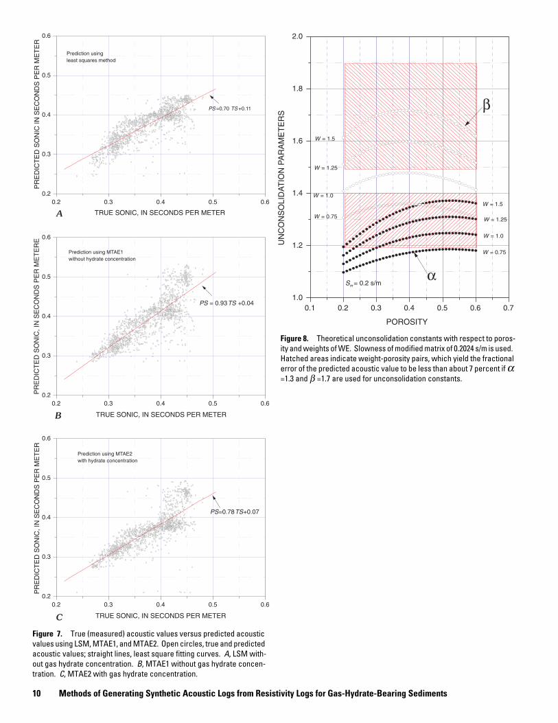
Comparison of three methods, least squares (LSM), MTAE1 without gas hydrate concentrations, and MTAE2 with gas hydrate concentrations is shown in figure 7, where measured acoustic values are plotted against the predicted acoustic values with the least squares linear fitting curves. The slope and inter-cept of the linear equation contain the information of the overall

performance of the various methods. Based on figure 7, we can say that overall, MTAE1 without gas hydrate concentrations works best for the Mallik 2L-38 well. However, when S>0.4 s/m, LSM works best, and when S<0.4 s/m, MTAE2 with gas hydrate concentrations works best for these data.

The only unknown parameter not able to be estimated from the resistivity log in applying MTAE1 or MTAE2 is the uncon-solidation parameter. If a few acoustic values for non-hydrate-bearing sediments are available close to the hydrate-bearing zone, we can estimate the unconsolidation constants by match-ing the velocities at the particular porosity (the average porosity is optimum) as explained in the previous section.

The fractional error of predicted acoustic values caused by the error in the unconsolidation constant in MTAE1 can be derived from equation (7), and it is given by

(12)

For MTAE2, the error function can be written as

(13)

The fractional error in the predicted acoustic value is propor-tional to the fractional error in unconsolidation constants. In

∆SS

------- ∆αα

-------=

∆SS

-------∆ββ

------- 1Sm

S------–

==

Figure 2. Comparison of P-wave velocities computed from weighted equation with W = 1.44 and modified time average equations with α = 1.3 and β = 1.68. Unconsolidation parameters were computed at 33 percent porosity.


900 950 1000 1050 11000.2

0.3

0.4

0.5

0.6

B

Mallik 2L-38

DEPTH, IN METERS

SO

NIC

, IN

SE

CO

ND

S P

ER

ME

TE

R

Observed Predicted from resistivity using LSM

1 10 100 10000.1

1

A

S=1.225 R-0.03878-0.743

Mallik 2L-38

RESISTIVITY, IN OHM-METERS

SO

NIC

, IN

SE

CO

ND

S P

ER

ME

TE

R

Observed Least squares fitting

order to evaluate the range of unconsolidation error introduced in the prediction, unconsolidation constants are computed from the definitions shown in equations (3) and (4) and are plotted with respect to the porosity and weights of WE (W = 0.75, W =

1.0, W = 1.25, and W = 1.5) in figure 8. As W increases, the unconsolidation constants increase. For a given weight, the variation of unconsolidation constant β is in the range of 0.1 and is between 0.1 (W = 0.75) and 0.2 (W = 1.5) for α. This

Figure 3. Prediction of acoustic values from resistivity log at Mallik 2L-38 well using least squares meth-od. A, Open circles, measured resistivity-acoustic values; solid circles, least squares curve. B, Measured (line) and predicted (open circle) acoustic values with respect to depth.

Discussion 7

900 950 1000 1050 11000.2

0.3

0.4

0.5

0.6

B

Mallik 2L-38

DEPTH, IN METERS

SO

NIC

, IN

SE

CO

ND

S P

ER

ME

TE

R

Observed P-wave sonic Predicted from resistivity using MTAE2

without gas hydrate concentration

900 950 1000 1050 11000.2

0.3

0.4

0.5

0.6

A

Mallik 2L-38


without gas hydrate concentration

DEPTH, IN METERS

SO

NIC

, IN

SE

CO

ND

S P

ER

ME

TE

R

figure indicates that the assumption that unconsolidation param-eters are constants irrespective of porosity is reasonable. If we assume that the error in α is 0.1 and α varies 1.2 to 1.4, then the possible fractional error in the acoustic value is 7 percent to 8.5 percent.

The predicted acoustic error owing to the error in β is less than that from the error in α. Let’s assume that the minimum value of Sm/S is about 0.5. Then the fractional error ∆S/S caused by ∆β/β is about half the error caused by ∆α/α . The

hatched regions in figure 8 show values of the weight-porosity pairs which yield fractional errors in acoustic values less than about 7 percent if α =1.3 and β =1.7 are used for unconsolida-tion constants for the prediction.

Pressure-temperature conditions control the occurrence of hydrate-bearing sediments. Because of the limited conditions of gas hydrate stability, hydrate-bearing sediments occur in shal-low depths, usually 500 to 1,500 m in permafrost regions and 200-1,000 m sub-bottom depth in deep marine environments.

Figure 4. Prediction of acoustic values from resistivity log at Mallik 2L-38 well using modified time average equations without gas hydrate concentration. A, using MTAE1; B, using MTAE2.


900 950 1000 1050 11000.2

0.3

0.4

0.5

0.6

B

Mallik 2L-38

DEPTH, IN METERS

SO

NIC

, IN

SE

CO

ND

S P

ER

ME

TE

R

Observed P -wave sonic Predicted from resistivity using MTAE2

with gas hydrate concentration

900 950 1000 1050 11000.2

0.3

0.4

0.5

0.6

A

Mallik 2L-38


with gas hydrate concentration

SO

NIC

, IN

SE

CO

ND

S P

ER

ME

TE

R

DEPTH, IN METERS

Therefore the range of porosity and the weight of WE applicable to hydrate-bearing sediments could be small; for example, at the Mallik 2L-38 well, porosity varies between 20 percent and 40 percent, and weight of WE varies between 1.44 and 1.6 depend-ing on the clay content (Lee and Collett, 1999).

Because of the shallow occurrence of hydrate-bearing sediments in the permafrost area, porosities and weights of WE may fall within the hatched region of figure 8. There-fore it is reasonable to assume that the unconsolidation con-stants estimated from the data at the Mallik 2L-38 well can be

Figure 5. Acoustic values predicted from resistivity log at Mallik 2L-38 well using modified time average equa-tions with gas hydrate concentration. A, using MTAE1; B, using MTAE2.

Conclusions 9

0.2 0.3 0.4 0.5 0.60.2

0.3

0.4

0.5

0.6

Mallik 2L-38

St=1.05Sw-0.01

PREDICTED SONIC USING WE, IN SECONDS PER METER

PR

ED

ICT

ED

SO

NIC

US

ING

MTA

E2,

IN S

EC

ON

DS

PE

R M

ET

ER

applied to other permafrost areas in the Arctic region without rendering significant errors to the prediction of acoustic values.

Conclusions

Methods of predicting acoustic logs from resistivity logs using modified time average equations are presented, for hydrate-bearing sediments. Unlike some other methods, clay terms are not included explicitly in the formulation, because it is assumed that the effect of the clay is manifested in the Archie’s constants and in the velocity of the modified matrix. All the parameters necessary for the transform can be estimated from the resistivity log except the unconsolidation constants.

When gas hydrate concentrations were not explicitly used in the prediction, using MTAE1 is better than using MTAE2, but using MTAE2 is better than using MTAE1 when gas hydrate concentrations were explicitly used in the prediction.

The range of unconsolidation constants to be used for hydrate-bearing sediments is small because the depths of

occurrence of hydrate-bearing sediments are shallow, restricted by the gas hydrate stability condition. Therefore the unconsolidation constants estimated at the Mallik 2L-38 well might be appropriate throughout the permafrost region in transforming resistivity logs into acoustic logs.

References Cited

Archie, G.E., 1942, The electrical resistivity log as an aid in determining some reservoir characteristics: Journal of Petroleum Technology, v. 5, p. 1–8.

Brito Dos Santos, W.L., Ulrych, T.J., and De Lima, O.A.L., 1988, A new approach for deriving pseudovelocity logs from resistivity logs: Geo-physical Prospecting, v. 36, p. 83–91.

Bussian, A.W., 1983, Electrical conductance in porous medium: Geo-physics, v. 48, p. 1258–1268.

Collett, T.S., Lewis, R., Dallimore, S.R., Lee, M.W., Mroz, T.H., and Uchida, T., 1999, Mallik 2L-38 downhole well log display-detailed evaluation of gas hydrate reservoir properties, in Dallimore, S.R., and others, eds., Scientific results from JAPEX/JNOC/GSC Mallik 2L-38 Gas Hydrate Research Well, Mackenzie Delta, Northwest Territories, Canada: Geological Survey of Canada Bulletin 544, p. 295–311.

Figure 6. Comparison of predicted acoustic values from resistivity log at Mallik 2L-38 well using WE and MTAE2 with gas hydrate concentration.


0.2 0.3 0.4 0.5 0.60.2

0.3

0.4

0.5

0.6

C

Prediction using MTAE2 with hydrate concentration

PS=0.78TS+0.07

TRUE SONIC, IN SECONDS PER METER

PR

ED

ICT

ED

SO

NIC

, IN

SE

CO

ND

S P

ER

ME

TE

R

0.2 0.3 0.4 0.5 0.60.2

0.3

0.4

0.5

0.6

B

Prediction using MTAE1without hydrate concentration

PS = 0.93TS +0.04


PR

ED

ICT

ED

SO

NIC

, IN

SE

CO

ND

S P

ER

ME

TE

RE

0.2 0.3 0.4 0.5 0.60.2

0.3

0.4

0.5

0.6

A

Prediction using least squares method

PS =0.70 TS +0.11


PR

ED

ICT

ED

SO

NIC

IN S

EC

ON

DS

PE

R M

ET

ER

0.1 0.2 0.3 0.4 0.5 0.6 0.71.0

1.2

1.4

1.6

1.8

2.0

Sm = 0.2 s/m

W = 0.75

W = 1.0

W = 1.25

W = 1.5

W = 1.5

W = 1.25

W = 1.0

W = 0.75

POROSITY

UN

CO

NS

OLI

DA

TIO

N P

AR

AM

ET

ER

Sα

β

Figure 7. True (measured) acoustic values versus predicted acoustic values using LSM, MTAE1, and MTAE2. Open circles, true and predicted acoustic values; straight lines, least square fitting curves. A, LSM with-out gas hydrate concentration. B, MTAE1 without gas hydrate concen-tration. C, MTAE2 with gas hydrate concentration.

Figure 8. Theoretical unconsolidation constants with respect to poros-ity and weights of WE. Slowness of modified matrix of 0.2024 s/m is used. Hatched areas indicate weight-porosity pairs, which yield the fractional error of the predicted acoustic value to be less than about 7 percent if α =1.3 and β =1.7 are used for unconsolidation constants.

References Cited 11

Faust, L.Y., 1951, Seismic velocity as function of depth and geologic time: Geophysics, v. 16, p.192–206.

Han, D.H., Nur, Amos, and Morgan, D., 1986, Effects of porosity and clay content on wave velocities in sandstone: Geophysics, v. 51, p. 2093–2105.

Kim, D.Y., 1964, Synthetic velocity log: Paper presented at 33rd Annual International SEG meeting, New Orleans.

Labo, J., 1987, A practical introduction to borehole geophysics: Society of Exploration Geophysicists, 330 p.

Lee, M.W., Hutchinson, D.R., Collett, T.S., and Dillon, W.P., 1996, Seismic velocities for hydrate-bearing sediments using weighted equation: Journal of Geophysical Research, v. 102, p. 20347-20358.

Lee, M.W., and Collett, T. S., 1999, Gas hydrate amount estimated from compressional- and shear-wave velocities at the JAPEX/JNOC/GSC

Mallik 2L-38 gas hydrate research well, in Dallimore, S.R., and oth-ers, eds., Scientific results from JAPEX/JNOC/GSC Mallik 2L-38 Gas Hydrate Research Well, Mackenzie Delta, Northwest Territories, Canada: Geological Survey of Canada Bulletin 544, p. 313–322.

Pearson, C.F., Halleck, P.M., McGuire, P.L., Hermes, R., and Mathews, M., 1983, Natural gas hydrate deposit—A review of in-situ proper-ties: Journal of Physical Chemistry, v. 97, p. 4180–4185.

Rudman, A.J., Whaley, J.F., Blakely, R.F., and Biggs, M.E., 1975, Trans-form of resistivity to pseudovelocity logs: American Association of Petroleum Geologists Bulletin, v. 59, p. 1151–1165.

Worthington, P.F., 1991, The integrity of pseudo-acoustic transforms: Scientific Drilling, v. 2, p. 279–286.

Wyllie, M.R.J., Gregory, A.R., and Gardner, G.H.F., 1958, An experimental investigation of factors affecting elastic wave velocities in porous media: Geophysics, v. 23, p. 459–493.

Methods of Generating Synthetic Acoustic Logs from ... · Methods of Generating Synthetic Acoustic...

Documents

Transcript of Methods of Generating Synthetic Acoustic Logs from ... · Methods of Generating Synthetic Acoustic...