Methods for Making Predictions - NASA (Goebel... · 2008-08-08 · Methods for Making Predictions:...

1

Prognostics and Health ManagementENME 808A – Fall 2007

guest lecture

Methods for Making Predictions: model based methods, data driven methods and hybrid approaches

Kai Goebel, Ph.D.NASA Ames Research Center

Prognostics Center of [email protected]

Work referenced in these slides was performed in large part while author was with GEIt contains material from public presentations made by the author and papers co-authored as well as material made available from other parties, including contributions by Piero

Bonissone, Bill Cheetham, Neil Eklund, Weizhong Yan and others from GE Global Research and George Vachtsevanos and Bhaskar Saha from Georgia Tech

See also list of references on last slide

Some Current NASA Activities in PHM

ROBOTIC SPACE FLIGHT

HUMAN SPACE FLIGHT

Ground Diagnostics for CLV and Ground Test / Integration Infrastructure

CLV Crew Abort Logic Development

Solid Rocket Motor Failure Detection

and Prediction

Data Analysis / Mining for Mission Ops

TacSat 3Intelligent Power ManagementGN&C Health ManagementAutomated Sensor Calibration

LCROSSGround-Based Root Cause

Determination; Data Analysis

AERONAUTICS

IVHMOn-board and off-board Diagnostics, Prognostics,

Logistics

Space StationFault

Analysis

Space Shuttle Main Engine Abnormal

Condition Detection

2

NASA Ames Prognostics CoE

• Umbrella for prognostic technology development in NASA’s health management activities.

• Organization– NASA Ames

• Intelligent Systems division (code TI)– Discovery and Systems Health (DaSH) area

» Approximately 70 people in five groups» Largest ISHM organization in NASA (nearly 60 engineers and researchers)» Consolidates all ISHM activity at ARC» Broad range of customers across NASA» Mid-TRL (3-7) technology development, maturation, and infusion » PCoE

• Addressing prognostic technology gaps within application areas– Aeronautics– Exploration science.

• Approximately 20 supporting members. • Strong affiliations with

– industry and academia through • Grants• Space Act Agreements• funded IPP, SBIR, STTR, and NRA projects• Internships

– Information exchange with other government organizations (National labs, DoD, …)

Prognostics CoE Activities

• Aeronautics Mission Directorate– Aviation Safety Program

• Integrated Vehicle Health Management (IVHM) program • CoE supports technology development for

– Actuators» EMA

– Electronic power supplies» Li-Ion batteries

– Avionics components

» Power semiconductors

– Aging Aircraft and Durability Program • Aircraft wiring health management.

– Model the characteristics of intact and damaged insulation and mechanisms to detect current damage and estimate impact of further deterioration.

3

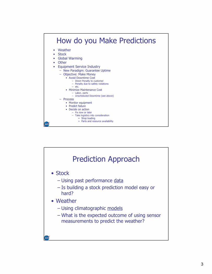
How do you Make Predictions• Weather• Stock• Global Warming• Other• Equipment Service Industry

– New Paradigm: Guarantee Uptime

– Objective: Make Money• Avoid Downtime Cost

– Direct Penalty to customer– Penalty due to safety violations– etc.

• Minimize Maintenance Cost– Labor, parts– Unscheduled Downtime (see above)

– Process• Monitor equipment• Predict failure• Decide on action

– Fix now or later– Take logistics into consideration

» Shop loading» Parts and resource availability

Prediction Approach

• Stock

– Using past performance data

– Is building a stock prediction model easy or hard?

• Weather

– Using climatographic models

– What is the expected outcome of using sensor measurements to predict the weather?

4

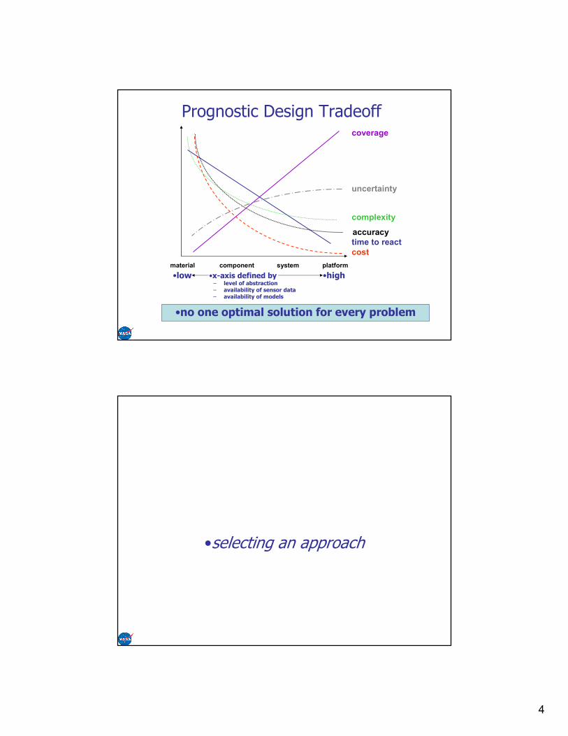
Prognostic Design Tradeoff

material component system platform

time to react

complexity

uncertainty

coverage

cost

•x-axis defined by– level of abstraction– availability of sensor data– availability of models

•high•low

•no one optimal solution for every problem

accuracy

•selecting an approach

5

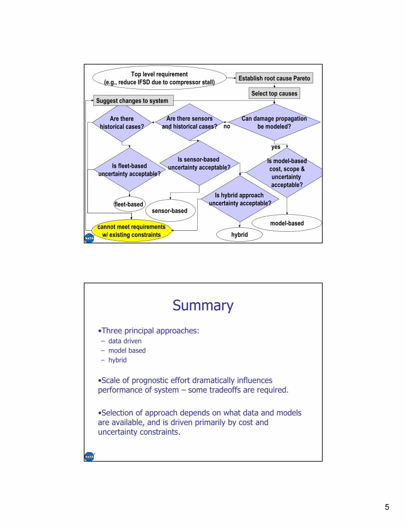
Top level requirement

(e.g., reduce IFSD due to compressor stall)Establish root cause Pareto

Select top causes

Can damage propagation

be modeled?

Are there sensors

and historical cases?

Are there

historical cases?

Is fleet-based

uncertainty acceptable?

cannot meet requirements

w/ existing constraints

Is sensor-based

uncertainty acceptable?Is model-based

cost, scope &

uncertainty

acceptable?

Is hybrid approach

uncertainty acceptable?sensor-based

fleet-based

hybrid

model-based

yes

no

Suggest changes to system

Summary

•Three principal approaches:

– data driven

– model based

– hybrid

•Scale of prognostic effort dramatically influences performance of system – some tradeoffs are required.

•Selection of approach depends on what data and models are available, and is driven primarily by cost and uncertainty constraints.

6

Data-driven Prediction Techniques

• Sensor-Based Conditioning

– Multi-Step Adaptive Kalman Filtering

– Auto-Regressive Moving Average Models

– Stochastic Auto-Regressive Integrated Moving Average Models (ARIMA)

– Forecasting by Pattern and Cluster Search

– Variants Analysis

– Parameter Estimation Methods

– Others


• Sensor-Based Conditioning (cont’d)– AI/CI Techniques

• Case-Based Reasoning• Intelligent Decision-Based Models• Min-Max Graphs• Support Vector Regression/Relevance Vector Regression

– Petri Nets– Soft Computing Tools

• Neural Nets

• Fuzzy Systems• Neuro-Fuzzy• Random Forests• …

7


•Fleet-based Methods

– Weibull-based lifing

– Survival analysis

– …

Model-based Approaches

•Micro-level models (materials-level)

– e.g.,:

• Crack growth models

• Spall growth models

•Macro-level models

– 1st principle models, e.g.,:

• Hot Gas Path cycle models

8

Hybrid Approaches

•Pre-Estimate Fusion of Model and Data

•e.g.,: – Using thermodynamic engine model and on-wing data for turbine damage propagation calculations

– Using battery model and impedance measurements for remaining life calculations

•Post-Estimate Fusion of Prognostic Estimates

•e.g.,:– Fuse model-based model output and data-driven model output to reduce prediction uncertainty for bearing spallprognostics

Methods for Making Predictions• Model-Based Methods

– Micro-level models (material-level)– Macro-level models (1st principle-level)

• Data-driven Methods– Sensor-Based Conditioning

• Regression• Case-based Reasoning• Neural Networks• SVM/RVM• Statistical Process Control• Random Forests• others

– Fleet-based Methods• Weibull-based lifing• Survival analysis• others

• Hybrid Approaches– Pre-estimate Fusion of Model and Data

• Example: Turbine component damage• Example: Battery health assessment

– Post-estimate Fusion of Model and Data• Example: Bearing spall

9

System

prognostics

•The onion of Fault Detection & Prediction

FaultsDetectable Fault

Isolatable Events

Trackable Events

Prognosable

Summary: Requirements

• Basic requirements for prognostics:1. Ability to describe system (component, …) health

a. sophisticated damage propagation model, or

b. collection of time series sensor measurements, plus a transfer function equating features to health

2. Definition of failure criterion (i.e., when is health = 0)

3. Assumptions about future usage (load, cycles, temp, …)

• Additional constraints:– Accurate determination of fault mode

• different fault modes will result in different propagation modes

– Ability to describe uncertainty of estimates

– Acceptable risk level

10

Tt

Diagnostic

Module

Prognostic

Module

(T=?)

Sensor

Data CBM

QUESTION: Once an impending failure is detected and identified, how can

we predict the time left before the failure occurs?

The Prognostic Module

11/29/200720

Spring Data•Experiment Force(newtons) Length(inches)

1 1.1 1.5

2 1.9 2.1

3 3.2 2.5

4 4.4 3.3

5 5.9 4.1

6 7.4 4.6

7 9.2 5.0

•What will the length be when the force is 5.0 newtons?

•What will the length be when the force is 10.0 newtons?

11

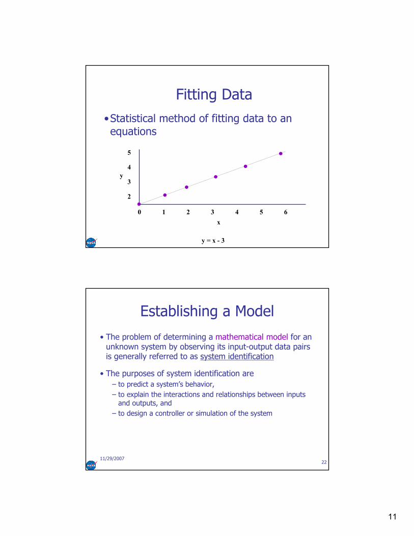
Fitting Data

•Statistical method of fitting data to an equations

5

4

3

2

0 1 2 3 4 5 6

y

x

y = x - 3

11/29/200722

Establishing a Model

• The problem of determining a mathematical model for an unknown system by observing its input-output data pairs is generally referred to as system identification

• The purposes of system identification are

– to predict a system’s behavior,

– to explain the interactions and relationships between inputs and outputs, and

– to design a controller or simulation of the system

12

11/29/200723

System Identification Process

– Structure and parameter identification may need to be done repeatedly

Specify model representing the system

(structure identification)

Optimize parameters

(parameter identification)

Conduct validation tests (Are tests satisfactory?)

Doneyes

no

Experiment/Collect Data

Prior Knowledge

11/29/200724

Structure Identification

•Determine the class of models within which the search for the most suitable model is conducted. y = f(u;θ) where u is the input vector and θ is the parameter vector.

•Example: Linear y= θ0 + θ1u1,

Second-order polynomial y= θ0 + θ1u1 + θ2u12

•If possible take advantage of domain knowledge

•Else use automated structure ID techniques

13

11/29/200725

Spring Example

•Structure Identification can be done using domain knowledge.

•The change in length of a spring is proportional to the force applied.

- Hooke’s law

length = k0 + k1 force

Hooke’s Law

• In physics, Hooke’s law of elasticity is an approximation which states that the amount by which a material body is deformed (thestrain) is linearly related to the force causing the deformation (the stress). – In most solids (and in most isolated molecules) atoms are in a state of

stable equilibrium.

• For systems that obey Hooke's law, the elongation produced is proportional to the load:– F=-kx

• where– x is the distance the spring is elongated by,– F is the restoring force exerted by the spring, and– k is the spring constant or force constant of the spring.

• When this holds, we say that the spring is a linear spring.

14

11/29/200727

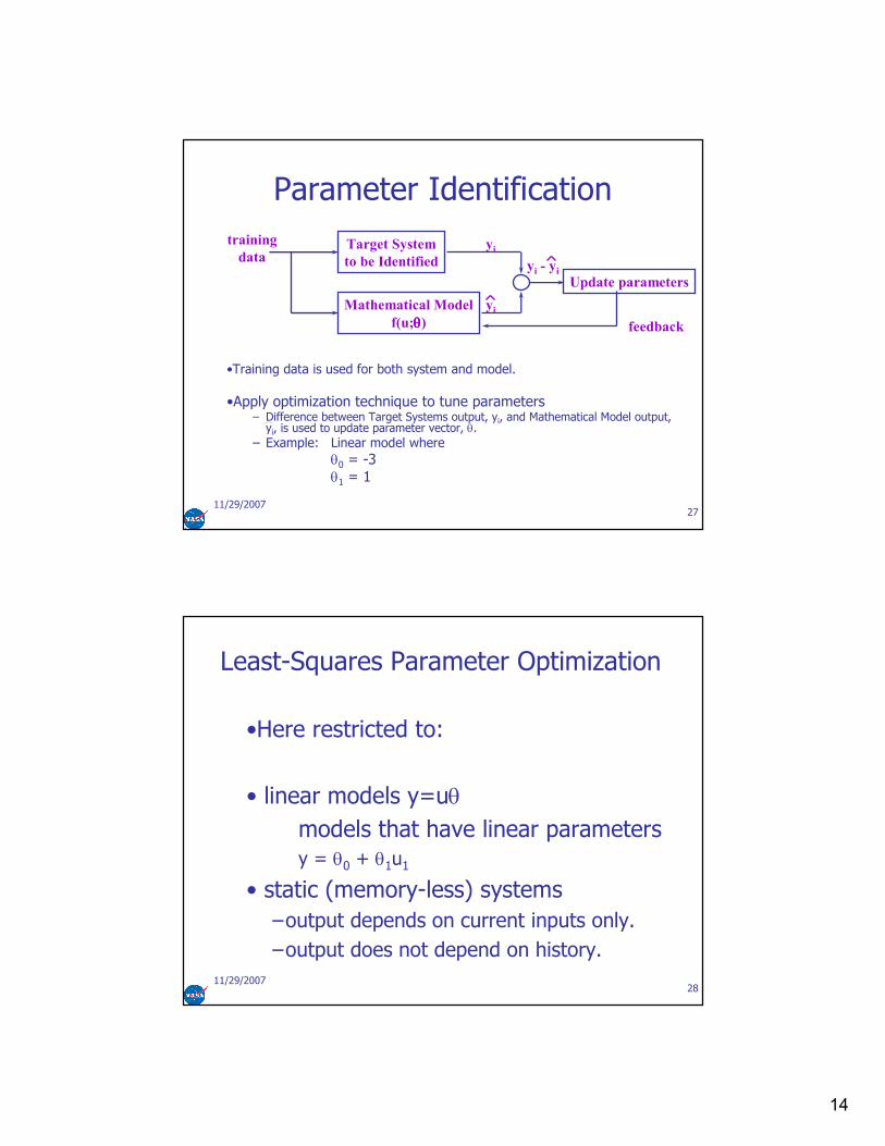
Parameter Identification

•Training data is used for both system and model.

•Apply optimization technique to tune parameters– Difference between Target Systems output, yi, and Mathematical Model output,

yi, is used to update parameter vector, θ.– Example: Linear model where

θ0 = -3θ1 = 1

Target System

to be Identified

Mathematical Model

f(u;θθθθ)

yi

yi

Update parameters

feedback

training

datayi - yi

11/29/200728

Least-Squares Parameter Optimization

•Here restricted to:

• linear models y=uθ

models that have linear parameters y = θ0 + θ1u1

• static (memory-less) systems

–output depends on current inputs only.

–output does not depend on history.

15

11/29/200729

Least-Squares: Error

•Least squared heavily penalizes error for data points that are far from the expected value

+3

+2

+1

0

-1

-2

-3

Expected

0 0 +1 0 -2 +3 0

0 0 1 0 4 9 0

Error

Error2

Sum of Squared Error = (0 + 0 + 1 + 0 + 4 + 9 + 0) = 14

11/29/200730

Least-Squares: Matrix method

• To uniquely identify the unknown vector θ it is necessary that – m (# of training items) >= n (# of parameters)

– training data is (ui;yi), i = 1, … , m

• If m = n , then we can solve for θ in y=Aθ usingθ = A-1 y

If m = n = 2 where f1(ui) = ui0 and f2(ui) = ui

1 then

f1(u1) f2(u1) 1 u1 y1A = = y =

f1(u2) f2(u2) 1 u2 y2

16

11/29/200731

Least-Squares: Matrix method (2)

•Example: Find a line from two points (1.1, 1.5), (1.9, 2.1)

A = 1 1.1 θ = θ1 y = 1.5

1 1.9 θ2 2.1

A-1 = 2.375 -1.375

-1.25 1.25

θ = A-1 y = 2.375 -1.375 1.5 = .675

-1.25 1.25 2.1 .75

y = .675 + .75x

11/29/200732

Least-Squares for m > n

•When m > n there are more data pairs than fitting parameters.

•An exact solution, satisfying all m equations, is not always possible.

•In order to handle this we need to incorporate an error vector.

Αθ + e = y

f1(u1) … fn(u1) θ1 e1 y1

+ =f1(um)

… fn(um) θn em ym

17

11/29/200733

Least-Squares: m > n (2)

•Best set of parameters θ is the one that minimizes the sum of the squared values of e.

•Error is minimized when

θ = (AT A)-1 ATy

11/29/200734

Spring Example

Αθ + e = y

1 1.1 e1 1.51 1.9 e2 2.11 3.2 e3 2.51 4.4 k0 + e4 = 3.31 5.9 k1 e5 4.11 7.4 e6 4.61 9.2 e7 5.0

k0 = (AT A)-1 ATy = 1.20k1 0.44

y = 1.2 + .44x

18

11/29/200735

Example: Spring data plot

•When force = 5, length = 1.2 + 5 * .44 = 3.4

Prediction (1)

0 1 2 3 4 5 6 7 8 9 101

1.5

2

2.5

3

3.5

4

4.5

5

5.5

6

•When force is 10, length = 1.2 + 10 * .44 = 5.6

19

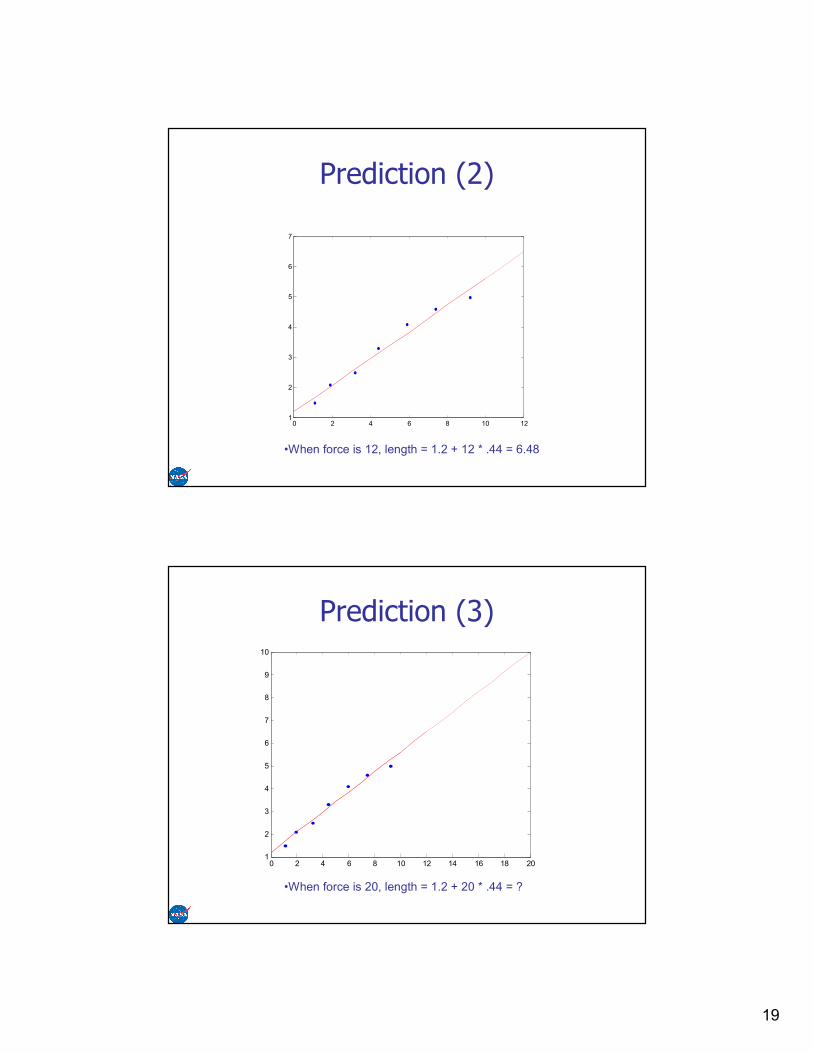
Prediction (2)

0 2 4 6 8 10 121

2

3

4

5

6

7

•When force is 12, length = 1.2 + 12 * .44 = 6.48

Prediction (3)

0 2 4 6 8 10 12 14 16 18 201

2

3

4

5

6

7

8

9

10

•When force is 20, length = 1.2 + 20 * .44 = ?

20

But

Hooke's law is only valid for the portion of the curve

between the origin and the yield point.

Stress-strain curve for low-carbon steel.

1. Ultimate strength

2. Yield strength

3. Rupture

4. Strain hardening region

5. Necking region.

Non-linear models

• Damage progressions often appears to have exponentially growing characteristics– Arrhenius law provides physical interpretation for temperature dependence of a chemical

reaction rate

– where• τ : Life span• Ea : Activation energy (eV)• T : Absolute Temperature (oK) • A : Constant• k : Boltzmann’s constant

– Assuming that we know the life span expectancy of a component at a given temperature Tnom, we can estimate the acceleration factor for health at a higher temperature Tstress using the above formula.

– Other acceleration factors:• where

– P=stressor (humidity, vibration, etc.)– a = stress-specific exponent

– Damage mechanics, Lemaitre 1992, etc.:

−

⋅= kT

Ea

eAτ

( )

−−

= stressnomB TTk

Ea

stressnom eTTAF

11

,

( )( )21

11 D

C

dN

dD Ptr

−+Γ=

+

γε γ

( )DfdN

dD,,εσ=

( ) ( )aPPfPAF stressnom ,,=

21

Bearings

• designed for “infinite” life

• fail due to hard particle contamination

(random occurrence)

Failure CriterionDestructive failure occurs when cage fails:

-In low speed bearings, spalls can cover entire race

-In high speed bearings, cage fails when spall

length >= circumferential ball spacing

Qualitative Analysis: Stress on cage crossbars and

rails increases dramatically when spall length > ball

spacing:

22

Materials-basedSpall Propagation Model

damage accumulation:

DSDS

=

( )( )21

11 D

C

dN

dD Ptr

−+Γ=

+

γε γ

( )εσ ,fdN

dD= ( )Df

dN

dD,,εσ=

Can’t measure damage directly in this application, need to select f that yields

correct propagation rate for test cases

Damage mechanics, Lemaitre 1992, etc.:

( ) ( )1 1

F

S D D

σσ = =

− −%

Images courtesy of Sentient Corporation

Steady-State RunsTest Runs

(variable load/speed)

Experimental Runs

23

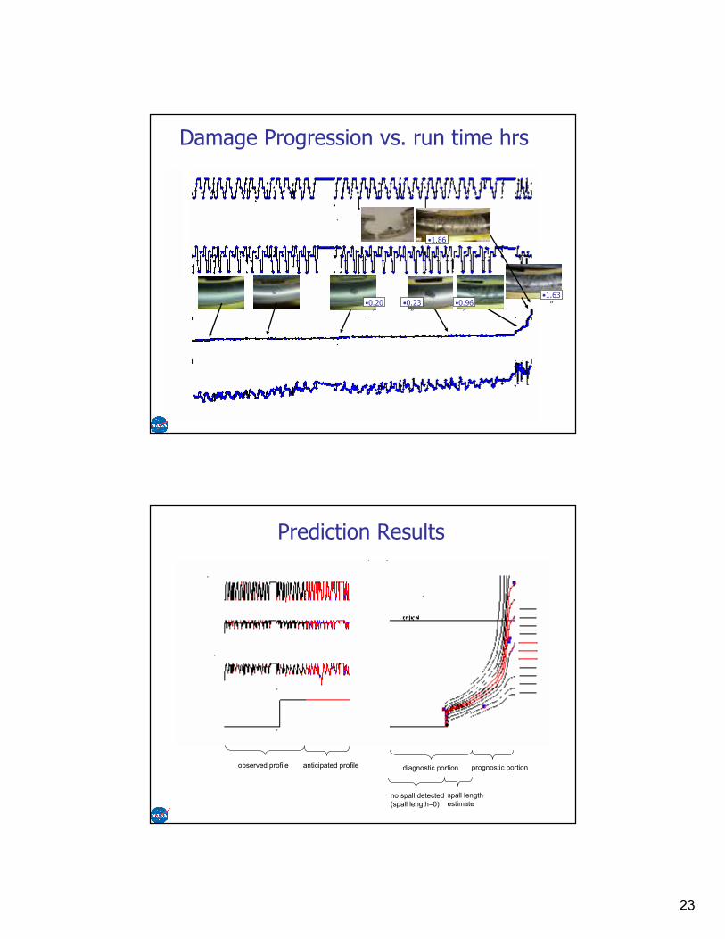
Damage Progression vs. run time hrs

•0.20”

•0.23”

•0.96”

•1.63”

•1.86”

Prediction Results

>> demo1

anticipated profileobserved profile

no spall detected

(spall length=0)

spall length

estimate

diagnostic portion prognostic portion

24

Non-linear Regression

0 10 20 30 40 50 600.84

0.86

0.88

0.9

0.92

0.94

0.96

0.98

Nonlinear fit may be appropriate here

time

he

alth

Damage Progression

• Many (not all) damage progressions appears to have exponentially growing characteristics

• But: pure data-driven approaches have their limits

– What is the offset (i.e., what prior damage exists)?

– What is the damage limit?

– What is the (exponential) model structure?

– What are the model parameters?

25

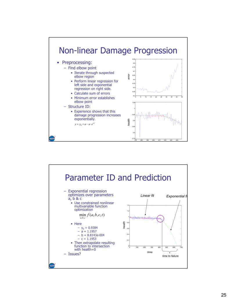
Non-linear Damage Progression

• Preprocessing:– Find elbow point

• Iterate through suspected elbow region

• Perform linear regression for left side and exponential regression on right side.

• Calculate sum of errors

• Minimum error establishes elbow point

– Structure ID:

• Experience shows that this damage progression increases exponentially.

ctbeaayy ⋅⋅−+= 0 health

0 5 10 15 20 25 30 35 40 458.4

8.45

8.5

8.55

8.6

8.65

8.7

8.75

8.8

8.85

370 380 390 400 410 420 430 4400.75

0.8

0.85

0.9

0.95

1

1.05

err

or

Parameter ID and Prediction

– Exponential regression optimizes over parameters a, b & c • Use constrained nonlinear multivariable function optimization

• Here– y0 = 0.9384– a = 1.1957– b = 8.8143e-004– c = 1.1953

• Then extrapolate resulting function to intersection with health=0

– Issues?

),,,(min,,

tcbafcba

0 100 200 300 400 500 600 7000

0.2

0.4

0.6

0.8

1

1.2

1.4

Linear fit Exponential fit

time

health

time to failure

26

Case-Based Reasoning for Forecasting

• Basic Hypothesis:

– Examples of cases that went to failure have a trail of characteristic features that describes them at each time step plus an associated remaining life.

– The comparison of a new example to old existing examples allows estimation of remaining life

52

What is CBR?

• A case-based reasoner solves new problems by using or adapting solutions that were used to solve old problems

• offers a reasoning paradigm that is similar to the way many people routinely solve problems

27

What Is CBR?

What is 12 x 12?

144

What is 13 x 12?

12 x 12 + 12

156

Who uses CBR?• Lawyers

– find previous ruling that applies to case

– show that it applies to current case

• Real Estate Appraiser

– find similar comparable houses

– estimate value of target based on value of comparable

• Diagnosticians

– Collect labeled data of normal data and faults (“cases”)

– Assess whether new data is similar to old cases

• Prognosticators

– Collect time series of data that went to failure (label is remaining life)

– Assess whether new data is similar to old case

28

55

ProblemThe Case-Based Cycle

56

PRIOR

CASES

CASE-BASE

Problem

RETRIEVERETRIEVE Similar

Cases

The Case-Based Cycle

29

57

PRIOR

CASES

CASE-BASE

Problem

RETRIEVERETRIEVE

Solution

RR

EE

UU

SS

EE

Similar

Cases


58

PRIOR

CASES

CASE-BASE

Problem

RETRIEVERETRIEVE

SolutionREVISEREVISESolution

RR

EE

UU

SS

EE

Similar

Cases


30

59

PRIOR

CASES

CASE-BASE

Problem

RETRIEVERETRIEVE

SolutionREVISEREVISE

RETAINRETAIN

RR

EE

UU

SS

EE

Similar

Cases


$

Solution

60

What is a Case?

• several features describing a problem (or a faulty equipment)

• plus an outcome or a solution (or remaining life)

• cases can be very rich

– text, numbers, symbols, plans, multimedia

• cases are not usually distilled knowledge

• cases are records of real events

• and are excellent for justifying decisions

31

61

How Does Retrieval Work?

• imagine a decision with two factors that influence it

• should you grant a person a loan?

net monthly income

monthly loan repayment

(more factors in reality)

62

How Does CBR Work? these factors can be used as axes for a graph

net monthly income

mont hly loan repayment

32

63

How Does CBR Work? a previous loan can be plotted against these

axes

net monthly income


64

How Does CBR Work?

and more good loans

net monthly income


33

65

How Does CBR Work?

plus some bad loans

net monthly income


66

How Does CBR Work?

a new loan prospect can be plotted on the

graph

net monthly income


new case

34

67

How Does CBR Work?

and the distance to its nearest neighbors

calculated

net monthly income


68

How Does CBR Work?

• the best matching past case is the closest

this suggests a precedent

the loan should be successful

35

11/29/200769

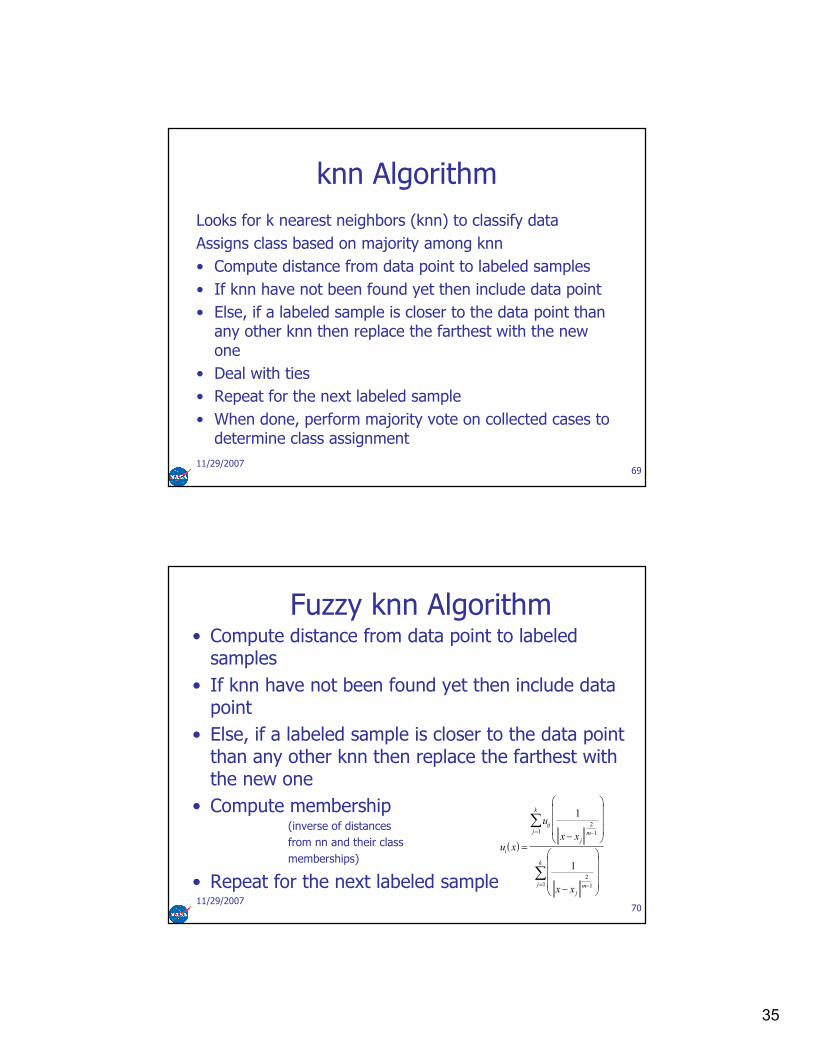
knn Algorithm

Looks for k nearest neighbors (knn) to classify data

Assigns class based on majority among knn

• Compute distance from data point to labeled samples

• If knn have not been found yet then include data point

• Else, if a labeled sample is closer to the data point than any other knn then replace the farthest with the new one

• Deal with ties

• Repeat for the next labeled sample

• When done, perform majority vote on collected cases to determine class assignment

11/29/200770

Fuzzy knn Algorithm• Compute distance from data point to labeled samples

• If knn have not been found yet then include data point

• Else, if a labeled sample is closer to the data point than any other knn then replace the farthest with the new one

• Compute membership(inverse of distances

from nn and their class

memberships)

• Repeat for the next labeled sample

( )u x

u

x x

x x

i

ijj

k

j

m

j

mj

k

=−

−

= −

−=

∑

∑

12

1

2

11

1

1

36

71

How Does CBR Work?

over time the prediction can be validated

net monthly income


it was a good loan

72

How Does CBR Work?

the system is learning to differentiate good

and bad loans better

net monthly income


37

73

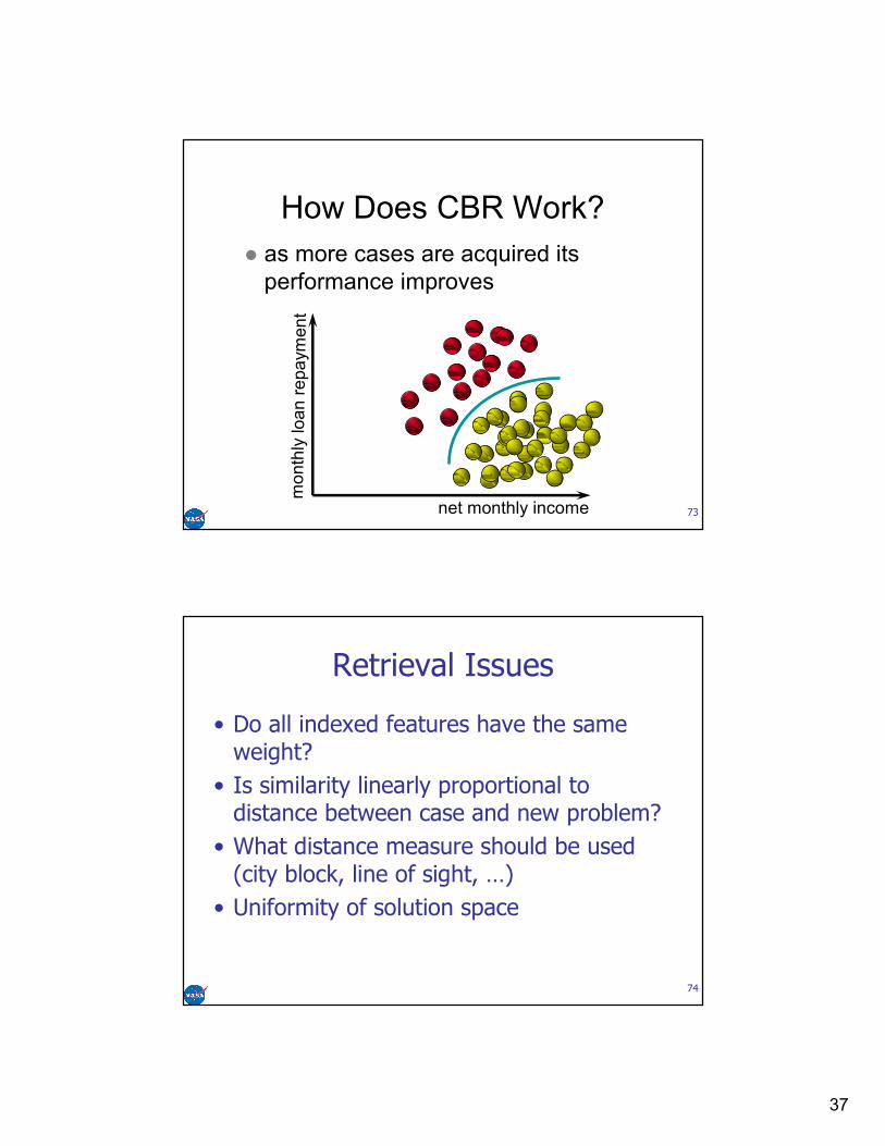
How Does CBR Work?

as more cases are acquired its

performance improves

net monthly income


74

Retrieval Issues

• Do all indexed features have the same weight?

• Is similarity linearly proportional to distance between case and new problem?

• What distance measure should be used (city block, line of sight, …)

• Uniformity of solution space

38

75

When to Apply CBR?

• when a domain model is difficult or impossible to elicit

• when the system will require constant maintenance

• when records of previously successful solutions exist

76

Case-Base Issues

• Number of cases needed

• Locally dense areas in CB vs. sparse areas

• Removing overlapping cases

• How to efficiently search

– create abstractions from cases

– multiple case bases

• Features used for indexing

• Weighting the features

• How to deal with evolving systems

39

77

Disadvantages of CBR

• Can take large processing time to find similar cases in case-base

• Can take large storage space for all the cases

• Cases may need to be created by hand

• Adaptation may be difficult

78

CBR Tradeoff

• if you require the best solution or the optimum solution - CBR may not be for you

• CBR systems generally give good or reasonable solutions

• this is because the retrievedcase often requires adaptation

40

Application to Locomotive Failure

• X = Age of locomotive, # of recommendations, miles/day, avg. megawatt hours, and many more.

• Y = Time to failure for that locomotive.

• We analyzed the performance of the evolutionary approach over two years of operation and maintenance data for a fleet of 1100 locomotives.

• The evolutionary algorithm automatically picked the best combination of variables from the X space that best allowed us to predict the time to failure.

• With passage of time, the genetic algorithm also automated the task of keeping the model trained without human intervention.

Top 20% reliability

Bottom 20% reliability

X = Asset History Y = Future Reliability

Loco Number: 5700

Design and Configuration

Type: AC4400

Electrical System: Bosch

…

Utilization Information

Age: 2.9 years

Mileage: 247,567 mi.

Average miles/day: 299

Maintenance Information

Time elapsed since last repair: 10 days

Median time between repairs 60 days

Median time from repair to next

recommendation (Rx) 52 days

We focus on selection of top 20%

Bonissone, P.P.; Varma, A.; Aggour, K.; A fuzzy instance-based model for predicting expected life: a locomotive application. IEEE International

Conference on Computational Intelligence for Measurement Systems and Applications, 2005. CIMSA. 2005 20-22 July 2005. pp.:20 - 25

41

Fuzzy Case-Based Model (FCBM)

x2

x1

Peers P(Q)xn

5

2b

otherwise 0

10 if

a

cx1

1

),,;(

>−

+=

−GBF

cbaxTGBFi

i

iiiiiii

1.0

0.0

0.2

0.4

0.6

0.8

c1

a1

b1

Probe Q XSpaceState

R1

Local Models

& Aggregation

y ii yX →

1) Retrieval of similar cases from

the Data Base

2) Evaluation of similarity

measure between the probe and the

retrieved cases

3) Local reasoning models give a

decision (Y) for each of the cases

4) Outputs Aggregation (weighted

by their similarities) as the final

decision (Y) for the probe Q

Reasoning process

Note:

This process is actually more correctly referred to as “Instance-Based Modeling”Bonissone, P.P.; et al., 2005

Neural Networks for Prognostics

42

11/29/200783

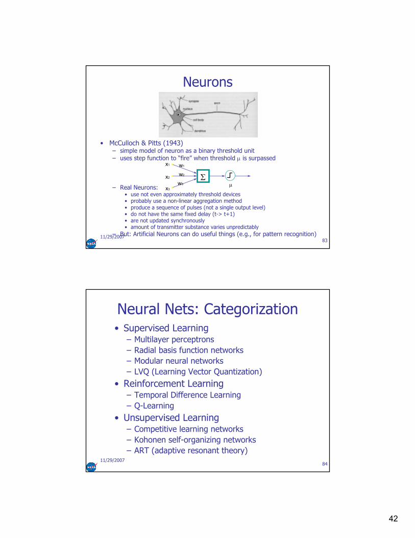
Neurons

• McCulloch & Pitts (1943)– simple model of neuron as a binary threshold unit

– uses step function to “fire” when threshold µ is surpassed

– Real Neurons:• use not even approximately threshold devices• probably use a non-linear aggregation method• produce a sequence of pulses (not a single output level)• do not have the same fixed delay (t-> t+1)• are not updated synchronously• amount of transmitter substance varies unpredictably

– But: Artificial Neurons can do useful things (e.g., for pattern recognition)

x1

x2

x3

w1

w2

w3 µΣ

11/29/200784

Neural Nets: Categorization• Supervised Learning

– Multilayer perceptrons

– Radial basis function networks

– Modular neural networks

– LVQ (Learning Vector Quantization)

• Reinforcement Learning– Temporal Difference Learning

– Q-Learning

• Unsupervised Learning– Competitive learning networks

– Kohonen self-organizing networks

– ART (adaptive resonant theory)

43

11/29/200785

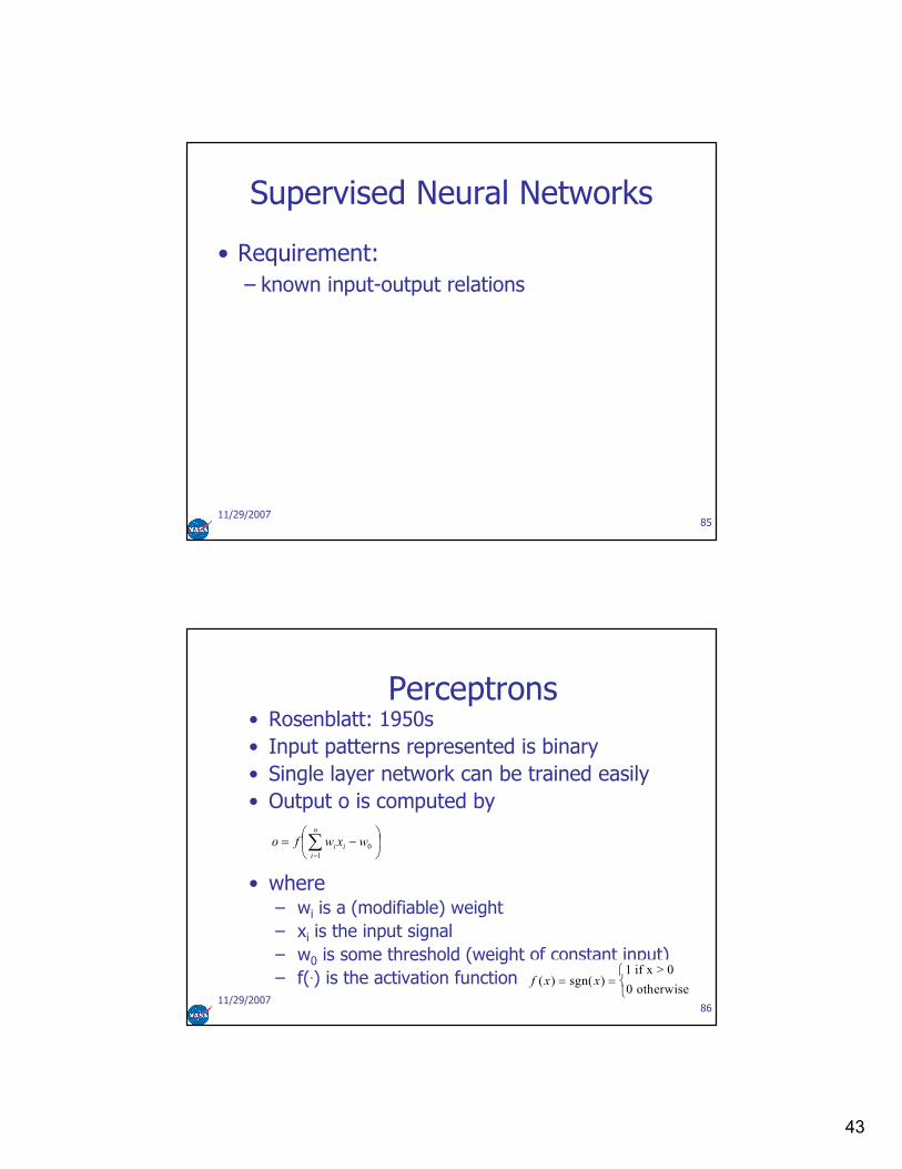
Supervised Neural Networks

• Requirement:

– known input-output relations

input pattern output

11/29/200786

Perceptrons• Rosenblatt: 1950s

• Input patterns represented is binary

• Single layer network can be trained easily

• Output o is computed by

• where– wi is a (modifiable) weight

– xi is the input signal

– w0 is some threshold (weight of constant input)

– f(.) is the activation function

−= ∑

=

n

i

ii wxwfo1

0

f x x( ) sgn( )= =

1

0

if x > 0

otherwise

44

11/29/200787

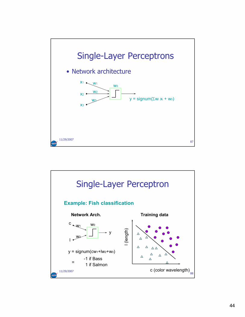
Single-Layer Perceptrons

• Network architecture

x1

x2

x3

w1

w2

w3

w0

y = signum(Σwi xi + w0)

11/29/200788

Single-Layer Perceptron

Example: Fish classification

c

l

w1

w2

w0

Network Arch.

y = signum(cw1+lw2+w0)

-1 if Bass

1 if Salmon=

y

Training data

c (color wavelength)

l (length)

45

11/29/200789

Perceptron Learning

• Learning:

– select an input vector

– if the response is incorrect, modify all weights

where

ti is a target output

η is the learning rate

∆w t xi i i= η

11/29/200790

XOR• Minsky and Papert reported a severe shortcoming of single layer perceptrons, the XOR problem…

not linearly separable

x1 x2 output

0 0 0

0 1 1

1 0 1

1 1 0

x

xO

O1

10

0

021021

01021

02021

0021

011

001

010

0000

wwwwww

wwwww

wwwww

wwww

−≤+⇔≤++

−>⇔>++

−>⇔>++

≤⇔≤++

x2

w1x1x3

w2

θ=-w0

46

11/29/200791

Enter the Dark Ages of NNs

• …which (together with a lack or proper training techniques for multi-layer perceptrons) all but killed interest in neural nets in the 70s and early 80s.

47

Two-Layer Perceptron: XOR

x2

+1

+1

1.5

-1

0.5

+1

+1 0.5

+1

x1

x4

x3

x5

• Multi-layer architectures can deal with XOR– Determining weights is painful

• Idea– find first derivative of the error wrt the weights,

– then move the weights a small amount towards a smaller error

– Can one take the first derivative for the architecture above?

• what alternative learning method could one employ?

11/29/200794

Multi-Layer Perceptrons

• Recall the output

• and the squared error measure

which is amended to

• and the activation function

or or

“squashing

functions”

• then the learning rule for each node can be derived using the chain rule...

o f w xi ii

n

= −

=∑ θ

1

( )E t op p p= −2

( )p

k

p

k

p

kk

n

E t o= −=∑

2

1

( )f xe x=

+ −

1

1( )f x

e

e

xx

x=−+

=

−

−

1

1 2tanh ( )f x x=

-10 0 10

-1

-0.5

0

0.5

1

y

-10 -5 0 5 10

-1

-0.5

0

0.5

1

48

11/29/200795

Backpropagation

• make incremental change in the direction dE/dw to decrease the error.

• The learning rule for each node can be derived using the chain rule...

• …to propagate the error back through a multi-layer perceptron.

∂∂

E

parameters

∆wE

wki

p

kip

= − ∑η∂

∂

-2 0 2-2

0

2

0

5

10

15

20

(a)

XY

Z

-3 -2 -1 0 1 2 3-2

-1

0

1

2

X

Y

(b)

11/29/200796

Multilayer Perceptrons (MLPs)

Learning rule:

• Steepest descent (Backprop)

• Conjugate gradient method

• All optim. methods using first derivative

• Derivative-free optimization

Network architecture

x1

x2

y1

y2

hyperbolic tangentor logistic function

49

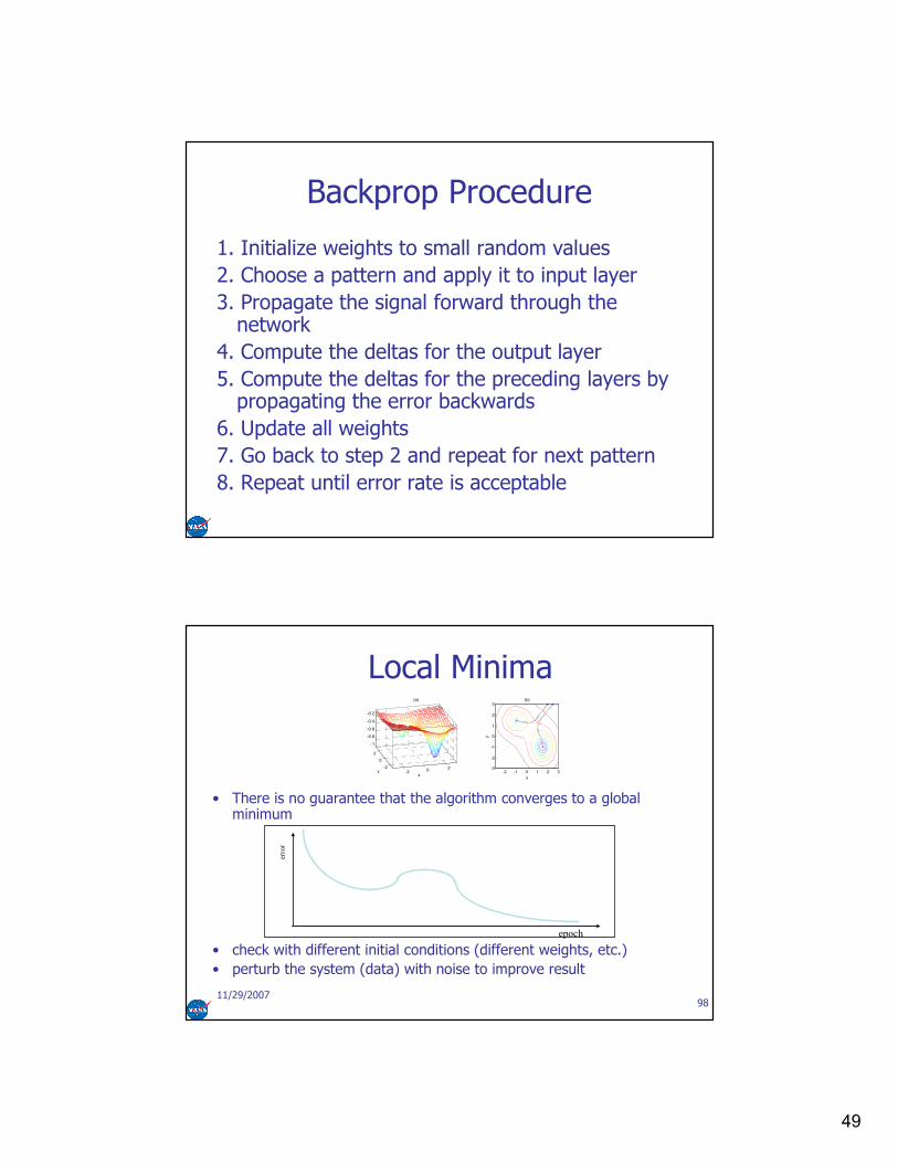
Backprop Procedure

1. Initialize weights to small random values

2. Choose a pattern and apply it to input layer

3. Propagate the signal forward through the network

4. Compute the deltas for the output layer

5. Compute the deltas for the preceding layers by propagating the error backwards

6. Update all weights

7. Go back to step 2 and repeat for next pattern

8. Repeat until error rate is acceptable

11/29/200798

-2 0 2-2

0

2

-1

-0.8

-0.6

-0.4

-0.2

x

(a)

y -2 -1 0 1 2 3-3

-2

-1

0

1

2

3

x

y

(b)

Local Minima

• There is no guarantee that the algorithm converges to a global minimum

• check with different initial conditions (different weights, etc.)

• perturb the system (data) with noise to improve result

epoch

error

50

11/29/200799

MLP Decision Boundaries

A B

B A

A

B

XOR Intertwined General

1-layer: Half planes

A B

B A

A

B

2-layer: Convex

A B

B A

A

B

3-layer: Arbitrary

Prognostics Example•Problem:

– Paper Making Machine standstill very costly

– If the user knew about an impending breakage, control parameters could be changed to avert the breakage

– many indicators

– poor indicators

– high noise

•Solution– Prognostics system using

a combination of techniques• data scrubbing

• variable reduction

• variable transformation

• model generation

• trending

• performance evaluation

51

Breakage Prediction Process

Datascrubbing

Datasegmentation

1 2

Data Reduction

Variableselection

PCA

3 4

Variable Reduction

Filtering Smoothing

5 6

Value Transformations Model Generation (1st Indicator)

CART8

Feature

Extraction

7

ClusteringNormali-zation

Transform-ation

Shuffling ANFIS Trending

9 10

11 13 14 15

Model Generation

(2nd Indicator)

12PerformanceEvaluation

Break

Indicator 1

Break

Indicator 2

Time to Breaks

Prediction

US5,942,689: System and method for predicting a web break in a paper machine, Bonissone, P., Chen, Y., Khedkar, P., 1999.

Pat. Pend.: Method for Predicting Time to Break Wet-End in Paper Mills Using Principal Component Analysis and Classification Trees", P. Bonissone, Y. Chen, filed 9/15/1999.

Pat. Pend.: Method for Predicting Time to Break Wet-End in Paper Mills Using Principal Component Analysis and Neuro Fuzzy Systems and Trending Analysis", P. Bonissone, Y. Chen,

filed 9/15/1999.

Pat. Pend.: System and method for improving Decision Trees by Bagging for Wet-End Web Breakage Prediction in Paper Mills", P. Bonissone, Y. Chen, 1999.

Graphical Description of the Prediction Error at time=60, i.e., E(60)

Actual

time-to-breaks

Predicted

time-to-breaks

E(0)

E(60)

60 min

90 min

120 min

time

Actual time of break

Time-to-breaks

52

Trending Analysis

Early Predictions:

Premature warning

may cause too many

corrections

No Predictions

E(60) [min]0 20 40- 20- 40- 60

Late Predictions:

Not enough time to take

corrective actions

Useful Predictions:

Enough time to take corrective actions

False PositiveFalse Negative

Lower limit

Definition of Useful Prediction: Limits for E(60)

Upper limit

53

Summary of E(60) Analysis

Early Predictions

(0)

No Predictions

(0)

E(60) [min]0 20 40- 20- 40- 60

Late Predictions

(1)

Correct Predictions

(24)

False PositiveFalse Negative

Lower limit Upper limit

Hybrid Approaches






54

Pre-Estimate Hybrid Fusion

• Problem constraints– Damage propagation model not available/too expensive

– Failure data not available

– Engine thermo-dynamic model available

– In-flight snapshot data available

• Challenge– Can one predict end-of-life of modules within engine due to component level faults?

System

…

Module X

Prognostics: Levels of Abstraction

Module A

parts

Vibration

data at high

sampling rate

Component Prog.

Damage

propagation

model

Physics-based life estimate

Inspection data

Component Prog.

Damage

propagation

modelOnce-per-flight

usage data

Physics-based life estimate

…

Engine

model

Once-per-flight

RMD data

Hybrid RUL

est.

Module X Prog.

55

Hybrid Prediction• What is hybrid here

• Use thermo-dynamic model to characterize module health• Challenge: what is end of life• Use operational margins as clue

• Use sensor data and feed through model to get current health state

• Then use updated nonlinear extrapolation to propagate damage and calculate time remaining

• Byproduct• No detailed materials knowledge required• Allows segregation of worsening faults vs. stable faults • Health estimate of component• Deterioration estimate• Root cause information

Component-level Prognostics: Approach

1. Off-line: Learn impact of faults– Model Faults with different magnitude in cycle deck

– Understand impact of faults• Expected sensor output

• Changes of performance characteristics

– Define health index as cumulative minimum operational margin

– Generate health index map for different components

cycle deck

Sensor readings

Parameter1 = f(fault1)Parameter2 = f(fault2)

…

Fault@limit

Normal

operation

Normal

operation

Deteriorated

engine

Operational margin 1

…

Operational margin n

OL

sensor

readings

cases

cases

cycle deck model

(NN, …)

Sensor readings

Parameter1 = f(fault1)Parameter2 = f(fault2)

…

health index (fault1),

health index (fault2)

…

sensor

readings

HI(Fi)

RM

cases

56

Component-level Prognostics Approach2. Online: Evolve component health

– Estimate deterioration– Find performance parameters that optimally

match sensor data– Calculate health index– Propagate health index forward by evolving fault

through non-linear regression

– RUL is intersection of health index at risk level cut-off

Real RM time series

(censored)model

(NN, …)

health index trajectories (fault1),

health index trajectories (fault2)…

Extrapolator RUL

RM

?

HI(Fi)

RUL

timetime

( ) ( )faultnowacceptable TTnowTHITRUL ˆ0ˆ ≥−=== σσ

0 50 100 150 200 250 3000

0.1

0.2

0.3

0.4

0.5

0.6

0.7

1

2

4

5

6

7

8

910

RUL

HI

Performance parameter 2

Performance parameter1

Performance Parameter 1

Performance

Parameter 2

State Assessmentsensor1 sensor2 sensor3 sensor4 sensor5 sensor6

Real sensor

measurements


Performanceparameter 2

• Generate response surfaces for module faults

• Normalize surfaces• Find performance parameter pair that best explains sensor datamin(Σwi*(Dist_i)^2),

i Є sensor1,

sensor2, sensor3,

sensor4, sensor5,

sensor6

Performance parameter 1 Performance parameter 1

Perform

ance parameter 2

Perform

ance parameter 2

Perform

ance parameter 2

Perform

ance parameter 2

Perform

ance parameter 2

Perform

ance parameter 2

Performance parameter 1Performance parameter 1 Performance parameter 1 Performance parameter 1

57

Real Example – Actuator failures

•This fault mode has consistent direction in performance parameter space•important diagnostic evidence for the fault mode

•Other fault modes are manifested by trajectories with different slope

•Rate of change is important prognostic information

•No additional specific materials/geometry/thermodynamics knowledge is used

Performance parameter1


Engine 1

Engine 2

Engine 3

Engine 4

Example Case (Real Data)

•Tracking component condition (health)

Com

ponent conditio

n (H

I)

cycles0 50 100 150 200 250 300 350 400 450 500 5500

0.2

0.4

0.6

0.8

1

Fault starts

diagnostic tool issues alert some time later

Maintenance

Without maintenance,

component health would have

further deteriorated

Potential remaining cycles after

maintenance

Potential remaining cycles after fault starts

58

Hybrid Approaches






Pre-Estimate Hybrid Fusion

• Problem constraints

– Lack of in-depth understanding of electro-chemical system

– Low-fidelity model

– Long-term aging data available

• Challenge

– Can one predict end-of-life of system

• Conditions are different than those seen in prior experience

• Significant uncertainties in model, sensor data, operating conditions

• Quantify uncertainties

59

Hybrid Prediction• What is hybrid here

– Use lumped parameter model to characterize battery health

– Use sensor data and feed through model to get current health state

– Use particle filter approach integrating future expected conditions to propagate damage and calculate time remaining

• Byproduct– Uncertainty estimates

– No detailed electro-chemical knowledge required

Battery Basics

• Impedance Z consists of: – resistance R, and

– reactance X

• (Z=R+jX)

concentration polarization

IR drop

activation polarization

Eo

increasing current I

increasing voltage E

Polarization Curve

+-

+-

e-

Load

Cathode

Anode

Electrolyte

Internal resistance increases as battery decays

Lumped parameter model used to predict response

Reelectrolyte

resistance

Cnfnonfaradic capacitance

RWWarburg impedance

RCTChargeTransfer Resistance

60

Measurement Scheme

Electrochemical Impedance Spectroscopy (EIS)

• Requires oscillator to carry out frequency sweep

• Plot capacitive vs. resistive component of cell– Interdependence of the components yields a semicircle

– Linear portion of curve corresponds to diffusion given by Warburg impedance

• Response is different in presence of passivation and

corrosion, providing a diagnostic for the health state of

battery

1/ωC

re re+rct

ωm=1/(rctCnf)

re+2S2Cnf

Electrolyte weakening Plate Sulfation Experiments (INL)

Re(Z)

Im(Z)

Increasing Ohmic Resistance

0

0

Re(Z)

Im(Z)

Increasing Charge Transfer Resistance

0

0

Bayesian Approach

• Relevance Vector Machine– State of the art in nonlinear probabilistic regression

– Faster than SVM

• Particle Filter– State of the art for nonlinear non-Gaussian state estimation

– Slower than Kalman Filter

– Uses model

61

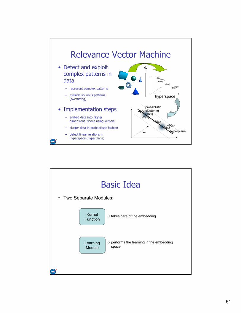
Relevance Vector Machine

• Detect and exploit complex patterns in data

– represent complex patterns

– exclude spurious patterns (overfitting)

• Implementation steps

– embed data into higher dimensional space using kernels

– cluster data in probabilistic fashion

– detect linear relations in hyperspace (hyperplane)

•Φ(x)

•Φ(x)•Φ(x)

•Φ(x)

•Φ(x)

•Φ(x)

Φ

...

hyperspace

probablisticclustering

hyperplane

•Φ(x)

•Φ(x)•Φ(x)

•Φ(x)

•Φ(x)

•Φ(x)

...

Basic Idea

• Two Separate Modules:

Learning

Module

Kernel

Function

performs the learning in the embedding

space

takes care of the embedding

62

KernelsKernels: A function that returns the value of the dot

product between the images of the two arguments

K(x1,x2)= <φ(x1),φ(x2)>

Simple examples of kernels:

K(x,z) = <x,z>d

K(x,z) = e-||x-z||2/2σ

Source: M. J. Tipping

• RVM is a sparse Bayesian model using the

same kernel basis as SVM

• Advantages

– Nuisance parameters can be integrated out

– Posterior probabilities generated

– Not limited to Mercer kernels

RVM: An Extension of SVM

63

Comparative Performance


Comparative PerformanceRegression

Classification


64

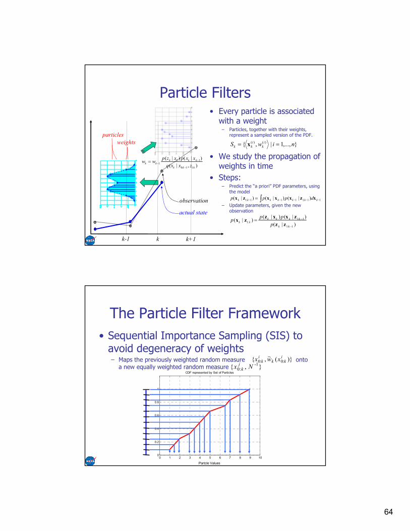
particles

weights

Particle Filters• Every particle is associated

with a weight– Particles, together with their weights,

represent a sampled version of the PDF.

• We study the propagation of weights in time

• Steps:– Predict the “a priori” PDF parameters, using

the model

– Update parameters, given the new observation

∫ −−−−− = 11:1111:1 )|()|()|( kkkkkkk dppp xzxxxzx

)|(

)|()|()|(

1:1

1:1:1

−

−=kk

kkkkkk

p

ppp

zz

zxxzzx

,...,1|, )()( niwS i

k

i

kk == x

actual state

observation

),|(

)|()|(

:11:0

11

kkk

kkkkkk

zxxq

xxpxzpww

−

−−=

k k+1k-1

The Particle Filter Framework

• Sequential Importance Sampling (SIS) to avoid degeneracy of weights– Maps the previously weighted random measure onto

a new equally weighted random measure

)(~, :0:0ikk

ik xwx

, -1:0 Nxjk

0 1 2 3 4 5 6 7 8 9 100

0.2

0.4

0.6

0.8

1

Crack Length [in]

CDF represented by Set of Particles

Partcle Values

65

∏∑

∫ ∏+

+=−+

=

+

+=−+

=

=

pk

kj

jj

i

kk

N

i

i

k

k

pk

kj

jjkkkpk

xxpxxpw

dxxxpzxpzxp

2

1

)(

1

1

)(

1

1:0:0

)|()|(~

)|()|()|(

Prognosis

• P-step ahead prediction defined by using the model update procedure in a recursive manner

The Particle Filter Framework

66

0 0.01 0.02 0.03 0.040

0.005

0.01

0.015

0.02

0.025

0.03

0.035

0.04

0.045

0.05

60% SOC EIS Impedance at 5 mV

Real Impedance (Ω)

Imaginary Impedance (-j Ω

)

Char

4-Wk

8-Wk

12-Wk

16-Wk

20-Wk

24-Wk

28-Wk

32-Wk

36-Wk

40-Wk

44-Wk

48-Wk

52-Wk

56-Wk

60-Wk

64-Wk

68-Wk Feature

Extraction

RVM

Regression

Model

Identification

EIS

Data

0.01 0.012 0.014 0.016 0.018 0.02 0.022 0.024 0.0260

1

2

3

4

5x 10

-3 60% SOC EIS Impedance at 5 mV (0.1-400 Hz)

Real Impedance (Ω)

Imaginary Impedance (- j Ω

) Ageing

Model Development

Feature

Extraction

PF

Tracking

PF

Prediction

EIS

Data

Impedance-

Capacity Mapping

Cause-Effect

Analysis

SOH SOC SOL

0 10 20 30 40 50 60 700

0.005

0.01

0.015

0.02

0.025Particle Filter Output

Time (weeks)

RE, RCT (Ω)

PF prediction

PF estimation

Measurements

RE

RCT

Fault Declared

0.015 0.02 0.025 0.03 0.035 0.040.65

0.7

0.75

0.8

0.85

0.9

0.95

1

Linear Fit on C/1 capacity vs. RE+R

CT

RE+R

CT (Ω)

C/1 (mAh)

Prognosis Framework

67

Remaining Useful Life

Summary and Final Remarks• Choice of prognostic technique must be based on constraints

– Model-based: need understanding of damage propagation

– Data-driven: need data time series to failure and failure criterion

• Techniques discussed today– Examples for physics-based models

– Particle filters

– Data-driven techniques• Regression (linear, nonlinear)

• Case-based reasoning

• Neural networks

• RVM

– Hybrid techniques• Pre-estimate fusion

• Issues requiring more research– Perception and state estimation

• Sensors are still the weak link

– Learning and adaptive systems• Space is the “final frontier” for ISHM

– Software complexity• V&V, certification

– Life estimation and physics of failure• Prognostics is still in its infancy

– Model building– Uncertainty management– Performance assessment

68

ReferencesK. Goebel and N. Eklund Prognostic Fusion for Uncertainty Reduction Proceedings of Infotech @ AIAA 2007

F. Xue, K. Goebel, P. Bonissone, W. Yan

An Instance-Based Method for Remaining Useful Life

Estimation for Aircraft Engines Proceedings of MFPT 2007 2007

H. Qiu, N. Eklund, W. Yan, P. Bonissone,

F. Xue, K. Goebel Estimating deterioration level of aircraft engines Proceedings of ASME Turbo Expo 2007 2007

X. Hu, N. Eklund, K. Goebel, and W.

Cheetham

Hybrid Change Detection for Aircraft Engine Fault

Diagnostics Proceedings of 2007 IEEE Aerospace Conference 2007

K. Goebel, H. Qiu, N. Eklund, W. Yan Modeling Propagation of Gas Path Damage Proceedings of 2007 IEEE Aerospace Conference 2007

P. Bonissone, K. Goebel, I. Naresh

Knowledge and Time: Selected Case Studies in

Prognostics and Health Management (PHM) Proceedings of IPMU '06 2006

N. Eklund and K. Goebel

Using Meta-Features to Boost the Performance of

Classifier Fusion Schemes for Time Series Data

Proceedings of International Joint Conference on

Neural Networks, 2006. IJCNN '06. pp. 3223 - 3230 2006

N. Iyer, K. Goebel, and P. Bonissone Framework for Post-Prognostic Decision Support Proceedings of 2006 IEEE Aerospace Conference 11.0903 2006

K. Goebel, N. Eklund, and P. Bonanni

Fusing Competing Prediction Algorithms for

Prognostics Proceedings of 2006 IEEE Aerospace Conference 11.1004 2006

N. Eklund and K. Goebel

Using Neural Networks and the Rank Permutation

Transformation to Detect Abnormal Conditions in

Aircraft Engines

Proceedings of the 2005 IEEE Mid-Summer Workshop

on Soft Computing in Industrial Applications, SMCia/05 pp. 1-5 2005

K. Goebel and P. Bonissone

Prognostic Information Fusion for Constant Load

Systems

Proceedings of the 7th Annual Conference on

Information Fusion, Fusion 2005, Vol. 2. pp. 1247 - 1255 2005

K. Goebel, P. Bonanni, N. Eklund

Towards an Integrated Reasoner for Bearings

Prognostics Proceedings of 2005 IEEE Aerospace Conference pp. 1 - 11 2005

W. Yan, K. Goebel, and C. J. Li

Flight Regime Mapping for Aircraft Engine Fault

Diagnosis

Proceedings of the 58th, Meeting of the Society of

Mechanical Failures Prevention Technology, Virginia

Beach, VA, April 26-30, 2004, Eds.: H. C. Pusey, S. C.

Pusey and W. R. Hobbs, MFPT, Winchester, VA pp. 153-164 2004

K. Goebel, N. Eklund, and B. Brunell

Rapid Detection of Faults for Safety Critical Aircraft

Operation 2004 IEEE Aerospace Conference Proceedings, vol. 5 pp. 3372 - 3383 2004

M. Krok and K. Goebel Prognostics for advanced compressor health monitoring

Proceedings of SPIE, System Diagnosis and

Prognosis: Security and Condition Monitoring Issues III,

Vol. #5107 pp.1-12 2003

P. Bonissone and K. Goebel

When will it break? A Hybrid Soft Computing Model to

Predict Time-to-break Margins in Paper Machines

Proceedings of SPIE 47th Annual Meeting, International

Symposium on Optical Science and Technology, Vol.

#4787 pp. 53-64 2002

P. Bonissone, K. Goebel, and Y. Chen Predicting Wet-End Web Breakage in Paper Mills

Working Notes of the 2002 AAAI symposium:

Information Refinement and Revision for Decision

Making: Modeling for Diagnostics, Prognostics, and

Prediction, Technical Report SS-02-03, AAAI Press,

Menlo Park, CA pp. 84-92 2002

• last slide

69

Internship Opportunities

• Perform research in prognostics at NASA Ames for a period from 3-12 months

• Contact [email protected]

Methods for Making Predictions - NASA (Goebel... · 2008-08-08 · Methods for Making Predictions:...

Documents

Transcript of Methods for Making Predictions - NASA (Goebel... · 2008-08-08 · Methods for Making Predictions:...