METHODS FOR DETERMINING TIME TO RETURN TO PLAY AFTER ...
108
University of Kentucky University of Kentucky UKnowledge UKnowledge Theses and Dissertations--Epidemiology and Biostatistics College of Public Health 2017 METHODS FOR DETERMINING TIME TO RETURN TO PLAY AFTER METHODS FOR DETERMINING TIME TO RETURN TO PLAY AFTER RECREATIONAL INJURY IN FIELD AND COURT SPORT ATHLETES RECREATIONAL INJURY IN FIELD AND COURT SPORT ATHLETES Sarah N. Morris University of Kentucky, [email protected] Author ORCID Identifier: http://orcid.org/0000-0002-7220-3291 Digital Object Identifier: https://doi.org/10.13023/ETD.2017.085 Right click to open a feedback form in a new tab to let us know how this document benefits you. Right click to open a feedback form in a new tab to let us know how this document benefits you. Recommended Citation Recommended Citation Morris, Sarah N., "METHODS FOR DETERMINING TIME TO RETURN TO PLAY AFTER RECREATIONAL INJURY IN FIELD AND COURT SPORT ATHLETES" (2017). Theses and Dissertations--Epidemiology and Biostatistics. 13. https://uknowledge.uky.edu/epb_etds/13 This Doctoral Dissertation is brought to you for free and open access by the College of Public Health at UKnowledge. It has been accepted for inclusion in Theses and Dissertations--Epidemiology and Biostatistics by an authorized administrator of UKnowledge. For more information, please contact [email protected].
Transcript of METHODS FOR DETERMINING TIME TO RETURN TO PLAY AFTER ...

University of Kentucky University of Kentucky
UKnowledge UKnowledge
Theses and Dissertations--Epidemiology and Biostatistics College of Public Health
2017
METHODS FOR DETERMINING TIME TO RETURN TO PLAY AFTER METHODS FOR DETERMINING TIME TO RETURN TO PLAY AFTER
RECREATIONAL INJURY IN FIELD AND COURT SPORT ATHLETES RECREATIONAL INJURY IN FIELD AND COURT SPORT ATHLETES
Sarah N. Morris University of Kentucky, [email protected] Author ORCID Identifier:
http://orcid.org/0000-0002-7220-3291 Digital Object Identifier: https://doi.org/10.13023/ETD.2017.085
Right click to open a feedback form in a new tab to let us know how this document benefits you. Right click to open a feedback form in a new tab to let us know how this document benefits you.
Recommended Citation Recommended Citation Morris, Sarah N., "METHODS FOR DETERMINING TIME TO RETURN TO PLAY AFTER RECREATIONAL INJURY IN FIELD AND COURT SPORT ATHLETES" (2017). Theses and Dissertations--Epidemiology and Biostatistics. 13. https://uknowledge.uky.edu/epb_etds/13
This Doctoral Dissertation is brought to you for free and open access by the College of Public Health at UKnowledge. It has been accepted for inclusion in Theses and Dissertations--Epidemiology and Biostatistics by an authorized administrator of UKnowledge. For more information, please contact [email protected].

STUDENT AGREEMENT: STUDENT AGREEMENT:
I represent that my thesis or dissertation and abstract are my original work. Proper attribution
has been given to all outside sources. I understand that I am solely responsible for obtaining
any needed copyright permissions. I have obtained needed written permission statement(s)
from the owner(s) of each third-party copyrighted matter to be included in my work, allowing
electronic distribution (if such use is not permitted by the fair use doctrine) which will be
submitted to UKnowledge as Additional File.
I hereby grant to The University of Kentucky and its agents the irrevocable, non-exclusive, and
royalty-free license to archive and make accessible my work in whole or in part in all forms of
media, now or hereafter known. I agree that the document mentioned above may be made
available immediately for worldwide access unless an embargo applies.
I retain all other ownership rights to the copyright of my work. I also retain the right to use in
future works (such as articles or books) all or part of my work. I understand that I am free to
register the copyright to my work.
REVIEW, APPROVAL AND ACCEPTANCE REVIEW, APPROVAL AND ACCEPTANCE
The document mentioned above has been reviewed and accepted by the student’s advisor, on
behalf of the advisory committee, and by the Director of Graduate Studies (DGS), on behalf of
the program; we verify that this is the final, approved version of the student’s thesis including all
changes required by the advisory committee. The undersigned agree to abide by the statements
above.
Sarah N. Morris, Student
Dr. Wayne T. Sanderson, Major Professor
Dr. Steven R. Browning, Director of Graduate Studies

METHODS FOR DETERMINING TIME TO RETURN TO PLAY AFTER RECREATIONAL INJURY IN FIELD AND COURT SPORT ATHLETES
_____________________________________
DISSERTATION
_____________________________________
A dissertation submitted in partial fulfillment of the requirements for the degree of Doctor of Philosophy in the College of Public Health at the University of Kentucky
By Sarah Nicole Morris
Lexington, Kentucky
Co-Directors: Dr. Wayne T. Sanderson, Professor of Epidemiology and Dr. Mary Kay Rayens, Professor of Biostatistics
Lexington, Kentucky
Copyright © Sarah Nicole Morris 2017

ABSTRACT OF DISSERTATION
METHODS FOR DETERMINING TIME TO RETURN TO PLAY AFTER RECREATIONAL INJURY IN FIELD AND COURT SPORT ATHLETES
An observational study was used to illustrate the application of time to event analysis methods to return to play; a secondary data analysis of athlete injury data from the High School RIOTM Injury Surveillance System (ISS) database was conducted. National Athletic Trainers’ Association (NATA)-certified athletic trainers from approximately 100 high schools in the US enroll their school in the system and complete the online “Exposure Report Form” for reportable injuries each week. New lateral ankle sprains and single-ligament knee injuries experienced by high school athletes during regularly scheduled participation in school-sanctioned sports for seven academic years (2005-2006 through 2011-2012) were analyzed. Field and court sport athletes (football, boys/girls soccer, volleyball, wrestling, basketball, baseball, and softball) were considered as these athletes were more likely to suffer lateral ankle or knee ligament sprains.
Detailed guidance was provided to assist athletic trainers and sports medicine researchers with understanding the appropriate data structure and programming statements required for time to return to play (T-RTP) analysis and the methodology appropriate for analyzing discrete time RTP categories. A data example was presented using lateral ankle sprain information to demonstrate how the life-table is useful for generating directly applicable information on expected T-RTP, and a discrete logistic regression model for this example highlights the relationship between severity of injury and T-RTP. Coding statements and life-table output were detailed for the LIFETEST procedure in SAS; SPSS instructions for generating life-tables were documented. The PHREG procedure in SAS using the TIES=DISCRETE option was presented to generate the discrete logistic regression model. An alternative method for computing hazard odds ratios was discussed to reduce computing time for large datasets with high numbers of tied event times using a pseudo dataset and the LOGISTIC procedure.
For 1st and 2nd degree lateral ankle sprains, the probability of RTP was highest 10-21 days after injury. For 3rd degree lateral ankle sprain, the probability of RTP was highest at least four weeks after injury. Gender had a marginal effect on RTP; male athletes were 18% more likely to return to play than female athletes. There was a significant interaction effect on RTP between time interval of return and ankle sprain severity. Athletes who
experienced a 1st degree sprain were 458% more likely to RTP in 1-2 days than athletes who experienced a 3rd degree sprain, and 2nd degree sprains were 259% more likely to RTP in 1-2 days than 3rd degree sprains. In general, 1st and 2nd degree LAS were more likely to return than 3rd degree sprains in the three weeks after injury.
Regardless of which knee ligament was injured, athletes had a very small chance of RTP within two weeks of injury. Athletes injuring the ACL any time during the season had only a 1 in 3 chance of returning before the end of the season. RTP probabilities increase slightly for PCL, LCL, and MCL injuries after two weeks. Athletes suffering a single-ligament knee sprain during competition were 25% less likely to RTP before the end of the season than athletes injured during practice. Gender did not have a significant effect on RTP. There was a significant interaction effect on RTP between time interval of return and injured knee ligament. Athletes who experienced ACL sprain were 78% less likely to RTP in 1-2 days than athletes with MCL sprain, 81% less likely to return in 3-6 days, 91% less likely to return in 7-21 days, and 74% less likely to return 4 weeks after injury. Athletes who experienced LCL sprains were 213% more likely to return in 1-2 days than athletes with MCL sprain, 73% more likely to return in 3-6 days, and 103% more likely to return in 7-9 days.
The literature on return to play has been largely descriptive in nature, and time to event analysis methodology has not been heavily utilized. The applied methods paper presented here provides sports medicine researchers with direction to apply the methodology and interpret the results. The findings suggest that ankle sprain severity has the strongest impact on RTP timelines. ACL sprains have the longest RTP times and athletes are not likely to return during the season; athletes who suffer MCL sprains could potentially return during the season, but can expect to be out a minimum of three weeks. These RTP probability estimates are directly applicable for use by coaches, athletic trainers, and other members of the sports medicine team as they help provide reasonable expectations for return time following injury and allow for more accurate RTP planning.
KEYWORDS: sports medicine, knee sprain, ankle sprain, time to return to play, life-table method, discrete logistic regression
Sarah Nicole Morris Student's Signature
April 14, 2017 Date
METHODS FOR DETERMINING TIME TO RETURN TO PLAY AFTER RECREATIONAL INJURY IN FIELD AND COURT SPORT ATHLETES
By
Sarah Nicole Morris
Wayne T. Sanderson, PhD Co-Director of Dissertation
Mary Kay Rayens, PhD
Co-Director of Dissertation
Steven R. Browning, MSPH, PhD Director of Graduate Studies
April 14, 2017

This dissertation is dedicated to my mom, Gina, a brilliant example of what a woman can accomplish; and to my dad, Mike, who would have enjoyed seeing this goal finally
achieved. Thank you for teaching me that I can do anything I set my mind to.
iii
Acknowledgements
My experience in this PhD program has been both challenging and rewarding. I will be
forever grateful for the mentoring from remarkable faculty and the opportunity to work
with such extraordinary students. I would like to thank my chair, Dr. Wayne Sanderson,
for stepping in at the last minute and helping me navigate toward the finish line. Your
guidance vastly improved the quality of this project and it is something I am very proud
of. To my co-chair, Dr. Mary Kay Rayens, there are not enough words to express my
gratitude for your teaching and encouragement throughout the years. You have been an
exceptional mentor and I appreciate your willingness to meet with me often and provide
useful feedback and helpful advice. Thank you to Dr. Steve Browning for keeping me on
track and asking those difficult questions that really forced me to think things through.
Dr. Carl Mattacola, thank you for so graciously welcoming a statistician into the world of
athletic training, answering countless questions, and opening doors for me to learn and
grow both academically and professionally. Dr. Heather Bush, you gave me direction
when I had none and provided inspiration and guidance to get this project started. Thank
you to Dr. Jennifer McKeon for introducing me to this project, offering numerous
research ideas, and providing access to relevant data sources. Thank you also to Dr.
Dawn Comstock from the University of Colorado Denver and the Colorado School of
Public Health for allowing the use of the High School RIOTM sports-related injury data.
Finally, I'd like to thank my family, especially my husband Adam and our son Oliver, for
their constant support and encouragement; you are the greatest blessings in my life.

iv
Table of Contents
Acknowledgements ............................................................................................................ iii
List of Tables ..................................................................................................................... vi
List of Figures ................................................................................................................... vii
1 Introduction ................................................................................................................. 1
1.1 Motivation for dissertation ........................................................................................ 3
2 Return to Play after Sports Injury: A Review of the Literature................................... 5
2.1 A decision-based return to play model ...................................................................... 5
2.2 Return to play in sports medicine literature .............................................................. 8
2.2.1 Literature search methodology ........................................................................... 8
2.2.2 Literature search results ...................................................................................... 9
2.3 Utilization of time to event analysis methods in current sports medicine literature 11
2.3.1 Literature search methodology ......................................................................... 12
2.3.2 Literature search results .................................................................................... 12
2.4 Epidemiology of ankle and knee sprains and return to play ................................... 15
2.4.1 Lateral ankle sprain .......................................................................................... 15
2.4.2 Knee ligament sprain ........................................................................................ 18
3 An Innovative Methodological Approach in Sports Medicine Research: Applying Time to Event Analysis to Return to Play ........................................................................ 24
3.1 Introduction ............................................................................................................. 24
3.2 Background ............................................................................................................. 25
3.3 Time to return to play analysis method ................................................................... 26
3.4 T-RTP example ....................................................................................................... 30
3.4.1 Design and sample ............................................................................................ 30
3.4.2 Measures ........................................................................................................... 31
3.4.3 Data analysis ..................................................................................................... 32
3.4.4 Results .............................................................................................................. 38
3.5 Discussion ............................................................................................................... 40
3.5.1 Return to play probabilities by ankle sprain severity ....................................... 41

v
3.5.2 Multivariate relationship between RTP, time and severity .............................. 42
3.6 Conclusion ............................................................................................................... 43
4 Return to Play Probabilities after Knee Injury in High School Athletes ................... 53
4.1 Introduction ............................................................................................................. 53
4.2 Methods ................................................................................................................... 56
4.2.1 Design and sample ............................................................................................ 56
4.2.2 Measures ........................................................................................................... 57
4.2.3 Data analysis ..................................................................................................... 58
4.3 Results ..................................................................................................................... 58
4.4 Discussion ............................................................................................................... 60
4.4.1 Limitations ........................................................................................................ 63
4.5 Conclusion ............................................................................................................... 64
5 Discussion and Conclusions ...................................................................................... 73
5.1 Summary ................................................................................................................. 73
5.2 Implications ............................................................................................................. 76
5.3 Strengths and limitations ......................................................................................... 77
5.4 Future research ........................................................................................................ 82
5.4.1 Parametric Accelerated Failure Time model .................................................... 82
5.4.2 Sports Medicine Research Institute .................................................................. 83
References ......................................................................................................................... 85
Vita .................................................................................................................................... 91

vi
List of Tables
Table 2.1 Types of injury and sports included in identified RTP literature (N=360 publications) ...................................................................................................................... 21 Table 3.1 Distribution functions for discrete time to return to play ................................. 44 Table 3.2 Estimated season start and end dates for field and court sports ........................ 44 Table 3.3 Demographic, injury, and competition characteristics for high school athletes with new lateral ankle sprain (N=2,086) .......................................................................... 45 Table 3.4 Estimated return to play probabilities by ankle sprain severity ........................ 46 Table 3.5 Discrete time logistic regression of return to play on time, injury severity, athlete demographics, and competition characteristics for lateral ankle sprains in high school athletes (n=5,132) .................................................................................................. 47 Table 4.1 Estimated season start and end dates for field and court sports ........................ 66 Table 4.2 Demographic, injury, and competition characteristics for high school athletes with new single-ligament knee sprain by injured ligament (N=1,049) ............................ 67 ACL=Anterior cruciate ligament; PCL=Posterior cruciate ligament; LCL=lateral collateral ligament; MCL=medial collateral ligament ...................................................... 67 Table 4.3 Estimated return to play probabilities by injured knee ligament ...................... 69 Table 4.4 Discrete time logistic regression of return to play on time, injured knee ligament, athlete demographics, and competition characteristics for new single-ligament knee sprains in high school athletes (n=3,852) ................................................................. 70 Table 4.5 Discrete time logistic regression of return to play on time, injured knee ligament, athlete demographics, and competition characteristics for new single-ligament knee sprains in high school football athletes (n=2,367) ................................................... 71 Table 5.1 Comparison of RTP Incidence Proportion (IP) to Lifetable RTP probabilities by ankle sprain severity .................................................................................................... 84

vii
List of Figures
Figure 2.1. Inclusion criteria and flow of retrieved articles .............................................. 22 Figure 2.2 Total number of publications by publication type ........................................... 22 Figure 2.3 Number of original research publications providing RTP criteria or guidance........................................................................................................................................... 23 Figure 3.1 HS RioTM ankle sprain data (First 20 records out of 2086) ............................. 48 Figure 3.2 SAS Life-Table for 1st degree ankle sprain in high school athletes ................ 48 Figure 3.3 Life-Table dialogue box in SPSS .................................................................... 49 Figure 3.4 SPSS Life-Table for 1st degree ankle sprain in high school athletes ............... 49 Figure 3.5 Original ankle sprain data and pseudo-observations for discrete logistic regression model ............................................................................................................... 50 Figure 3.6 Maximum likelihood estimates of Discrete-Time Logistic Model for HS RioTM ankle sprain data ............................................................................................................... 51 Figure 3.7 Cumulative RTP probabilities by lateral ankle sprain severity in high school athletes .............................................................................................................................. 52 Figure 4.1 Cumulative RTP probabilities by sprained knee ligament in high school athletes .............................................................................................................................. 72

1
1 Introduction
Ankle and knee injuries are ubiquitous with sports participation and account for up to
60% of all injuries that occur during play [1-3]. Ankle and knee sprains are the most
common injuries among athletes of all ages [4-7] across all sports [1]. An initial question
after an athlete sustains an injury is when they will be cleared to return to play (RTP).
The extent of tissue damage and tissue healing timelines are not direct indicators of how
long an athlete will be withheld from play, and many RTP decisions focus on resolving
the symptoms. However, symptom and function resolution can follow a vastly different
timeline than tissue healing, making a prognosis of time to RTP difficult. Current clinical
predictions of when an athlete will return to play after ankle and knee injuries are likely
to be misleading and erroneously underestimate RTP timelines in instances where a lack
of follow-up data excludes athletes from analysis. Current RTP estimations are
predominantly based on subjective reports of the individual patient’s symptoms and
anecdotal, expert opinion of clinicians. While neither of these approaches are incorrect,
there is limited clinical epidemiological research evidence to substantiate current RTP
predictions for ankle and knee injuries [8]. There are few prognostic indicators for these
injuries for determining when RTP will occur. This can potentially contribute to poor
compliance with rehabilitation programs due to athletes pushing for earlier RTP, setting
the athlete up for subsequent injury or increasingly severe injuries. Recurrent knee and
ankle injuries can lead to concomitant long-term health issues such as degenerative joint
diseases like osteoarthritis (OA). Ligament damage to the ankle or knee will likely result
in early-onset, post-traumatic OA, most often within 10 to 20 years after initial injury [9,
10]. For high school or college athletes suffering ankle or knee injuries, this indicates
2
they could suffer degenerative conditions by as early as 30 years old. While OA is
generally considered a factor of old age characterized by joint pain, swelling, limited
motion, and disability [11], young athletes are at risk for early-onset consequences
associated with ankle and knee joint injuries. Individuals suffering from posttraumatic
OA are typically younger patients, and the condition is significantly associated with
decreased physical activity, obesity, cardiovascular disease, and depression stemming
from loss of function and disability due to injury to the affected joint [12, 13]. With
approximately 30 million youth between the ages of 5 and 18 years in the US
participating in organized sports [7], the potential is quite high for young athletes to
suffer acute sports-related injuries or overuse injuries. It is estimated that 38% of high
school athletes will suffer sports-related injuries requiring treatment by a physician [7];
however, actual percentages may be higher due to underreporting or failure to seek
treatment [14].
To address these potentially significant public health issues related to knee and ankle
sprains among high school athletes, there is a need for the development of effective
strategies to diminish the impact of joint injuries, improve compliance with rehabilitation
programs, and reduce the risk of reinjury, with the goal of avoiding long-term effects
from injury and the continued maintenance of joint health. It is critical that athletic
trainers, doctors, and coaches be able to accurately gauge when an athlete should return
to play.
The purpose of this dissertation is to review the existing literature related to RTP after
ankle and knee sprain, identify factors that affect RTP timelines, and generate evidence-
based, objective prognostic indicators of when an athlete is likely to return to

3
participation using time to event analysis methodologies. The specific aims of this study
are:
1. Examine return to play and the use of time to event analysis methodology in
existing athletic training and sports medicine literature.
2. Provide guidance on generating and reporting return to play probabilities
using time to event analysis methodology for athletic trainers and sports medicine
researchers.
3. Analyze return to play probabilities for lateral ankle sprain and single-
ligament knee injuries in high school athletes participating in field and court
sports.
1.1 Motivation for dissertation
Return to play has historically been determined using subjective reasoning; there is a
need for more objective methods to assist in the determination of RTP [8]. Typical
research studies involving RTP report rates or proportions, but these measures can be
inaccurate in instances where a lack of follow-up data excludes some athletes from
analysis. Time to event analysis is a commonly used statistical analysis method that can
provide more accurate estimates for time to return to play (T-RTP) by accounting for all
injured athletes regardless of lack of follow-up concerning RTP. These analysis
techniques have commonly not been applied or related to RTP, and will provide athletic
trainers, coaches, and team physicians a more accurate way to estimate return.
Traditionally, time to event analyses have been aimed at estimating probabilities of
negative events such as death, recurrence of illness, or recidivism. In the sports medicine

4
setting the return to play event is positive, requiring a shift in the interpretation of time to
event analysis results. These analysis techniques will be used to conduct a secondary
analysis on data from the High School RIO (Reporting Information Online)TM Injury
Surveillance System (ISS) database regarding ankle and knee sprains in an attempt to
explore the best way to summarize return and inform RTP decisions. The probability
estimates will provide the predictive probability for how long until an athlete with
varying demographics and injury characteristics will RTP. The use of the High School
RIO TM ISS database for the purpose of evaluating RTP probabilities is approved under
the University of Kentucky Institutional Review Board Exemption Certificate for
Protocol #12-0409-X2H.

5
2 Return to Play after Sports Injury: A Review of the Literature
2.1 A decision-based return to play model
A predominant issue among sports medicine researchers related to return to play is the
subjective nature in which RTP decisions are made. There is a high degree of variability
among clinicians regarding factors considered for RTP [15], resulting in a call to develop
an objective method to determine RTP. One validated decision-based model proposes a
three-step process that requires the evaluation of health status (step 1), participation risk
(step 2), and consideration of decision modifiers (step 3) [16, 17]. Health status of the
athletes is based on medical factors such as patient demographics, symptoms, and clinical
injury evaluation. These measures tend to be more objective relative to those in
subsequent steps of the process. The evaluation of participation risk includes
consideration of sport risk modifiers and provides more information about the type of
sport, position played, competitive level, and the potential for utilization of protective
equipment. However, general historical information about the injury is not considered in
this step of the process. The consideration of decision modifiers allows for the influence
of outside factors surrounding the athlete. Internal and external pressure [18], timing of
the season, financial considerations, and fear of litigation are potential decision
modifiers; the balance between risk and benefit of participation should always be
considered when evaluating these factors.
Evaluation of health status is likely the first step taken by all athletic trainers and
clinicians when assessing an injured athlete; however, this decision model provides
specific factors to consider. Patient demographics and medical history, particularly
regarding previous sports-related injuries to determine first or subsequent injury, provides

6
a context in which injury signs and symptoms can be evaluated [16]. In addition to pain,
muscular strength and range of motion are the dominant health status factors assessed
through functional tests to determine return to play potential; it is suggested that both be
at or near preinjury levels before return is allowed, in a range of 70-100% [16, 19, 20].
The injury site should also be functionally stable with no tenderness, swelling, or effusion
[16]. Girth should also be evaluated, although no criteria has been suggested for a RTP
decision [16]. Appropriate laboratory tests should be conducted and reviewed to
objectively evaluate tissue healing or identify physiological abnormalities if present [16].
Often overlooked, psychological state, in particular, readiness and confidence, is an
important factor to consider when evaluating RTP [16]. Motivation during recovery has
been shown to increase satisfaction with recovery outcomes [21]; apprehension and
anxiety have been linked with higher rate of subsequent injury and shown to decrease
performance [22].
The evaluation of participation risk relies on specific sports-related information. Type of
sport, position played, and competition level should be considered [16]. In addition, the
ability to protect the injury must also be evaluated [16]. This is not only related to
protective equipment required for participation in the specific sport, but the ability to
provide isolated protection to the injury itself. Taping, bracing, and splinting may be
accommodated; however, athletes must adhere to the rules of their sport. This step is the
most subjective of the three-step decision model as a standardized method to evaluate
participation risk based on these sport-specific risk factors neither exists nor has been
proposed. Further, participation risk should also be evaluated based on injury-specific
risk factors. The risk of subsequent injury when a player is returned too early is certainly

7
important, but more essential, evidence regarding appropriate return timelines based on
historical empirical evidence should be considered.
While the evaluation of participation risk is specific to the sport and injury, the final step
of considering decision modifiers is the most specific to the individual athlete. Decision
modification factors are those that are not related to health, sport, or injury, but can
heavily influence a RTP decision. Both pressure from the athlete and external pressure
from coaches, teammates, family, fans, and media can encourage an athlete to return to
play too early. Time of season is suggested as a decision modifier [16], but it would have
a better fit within the context of participation risk. For example, it could be argued that
participation in an exhibition game would not pose as much of a risk to the athlete as
participation in a play-off game. Other suggested decision modifiers are related to
professional rather than recreational athletes. Conflict of interest, most common to paid
clinicians, and fear of litigation for damages resulting from RTP too early [16] should be
considered, but will likely not be factors for recreational athletes.
Validation of the proposed three-step RTP decision model indicated that in general sport
participation restrictions increased as injury severity increased [17]. However,
considerable heterogeneity in recommended restrictions was reported from the validation
study, likely from varying interpretation of participation risk. This is further evidence
indicating the need for objective methods to evaluate the risk of participation.
This decision-based model is an important first step toward providing an ordered process
in which clinicians can evaluate evidence leading to a RTP decision, and helps reduce the
influence of clinical experiences. While the model does propose a more objective
process, the evaluation of participation risk remains subjective in nature and lacks
8
empirical historical epidemiological data specific to the injury. If clinicians were
provided probability estimates summarizing timeframes in which athletes with specific
injuries return to play, they would have stronger evidence to make a determination of
participation risk.
2.2 Return to play in sports medicine literature
The ability to return to play has long been a pivotal question posed by athletes and
coaches after injury. Clinicians have relied on their personal experience to predict when
an athlete might return, and RTP decisions vary tremendously between clinicians [15].
Sports medicine researchers have recently called for a consensus on RTP guidelines and
criteria [23, 24], and researchers are beginning to answer that call.
2.2.1 Literature search methodology
Sports medicine literature published through October 2016 was searched using Medline
through PubMed and SPORTDiscus and CINAHL through EBSCOhost. Search terms
consisted of “return to play” in the title for all search engines and databases; for the
CINAHL search, “sports medicine” was selected as the special interest. PubMed returned
306 results, SPORTDiscus returned 272, and CINALH returned 81. After removing
duplicate publications, the remaining articles were manually evaluated for English
language and relevance to return to play in athletes after injury. A total of 360
publications were identified for review; publications were categorized as books, reviews
(book, clinical, comprehensive, narrative, literature, and systematic reviews and meta-
analyses), editorials (editorial articles, comments, and conference proceedings), and
original research. Publication identification is summarized in Figure 2.1.

9
2.2.2 Literature search results
To analyze the progression of sports medicine literature related to return to play, the trend
in number of publications per year by publication type was evaluated. The earliest
publication identified related to return to play was original research published in 1981
[25], detailing musculoskeletal profiling in terms of rehabilitation. There was only one
other publication from the 1980’s, conference proceedings from 1984 discussing shoulder
rehabilitation after rotator cuff tendonitis [26]. Return to play literature was published
every year beginning in 1991; only publications identified between 1991 and 2016 were
included when assessing trends over time. The identified publications address several
specific types of injures, as well as several different sports; these specifications are
summarized in Table 2.1.
The number of articles within each publication type for each year from 1991 to 2016 are
illustrated in Figure 2.2. Books, editorials, and reviews represent such a relatively small
number of the total publications identified (collectively only 43 of 360 publications, or
12%) that an emerging trend is difficult to identify. However, it is clear that in general
original research publications have seen an increase, particularly since 2010.
The original research publications were further evaluated to determine if they provided an
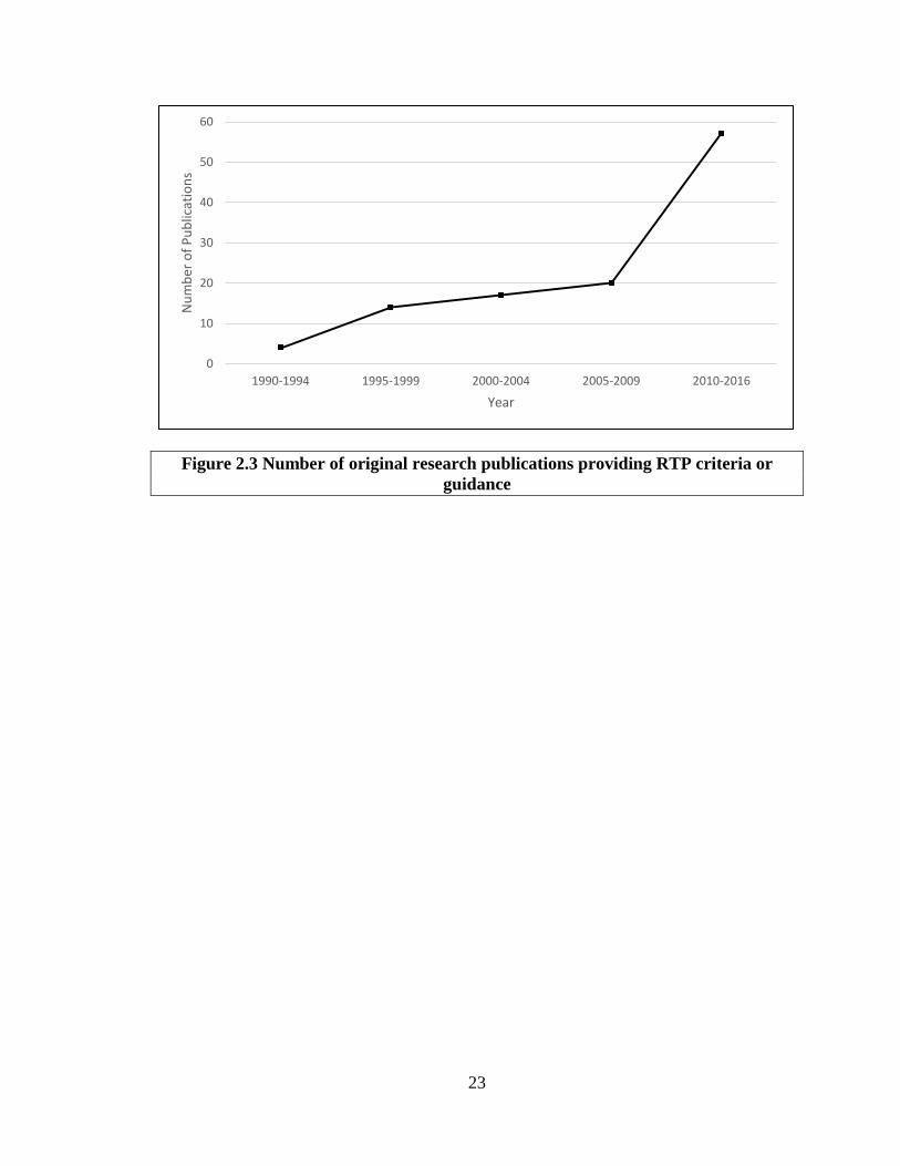
outline for return to play criteria or guidance. Figure 2.3 illustrates the trend over time in
number of publications providing RTP guidance, either to general athlete injuries,
specific injuries, or specific sports. For ease of illustration, publications from 2015 and
2016 have been included with publications from 2010 through 2014 in this figure; 40
articles were published between 2010 and 2014 and 17 articles were published in 2015

10
and 2016. The number of publications outlining RTP criteria or guidance has been
increasing since 1991, with a particularly large increase since 2010.
Evidence suggests that sports medicine researchers are now beginning to examine return
to play after injury more thoroughly. Not only has the number of publications related to
RTP increased, particularly since 2010, but the number of publications outlining RTP
criteria or guidance on RTP has increased as well. Nearly all of the articles that provide
estimates of return timelines present common epidemiological rates and proportions; the
epidemiological incidence proportion is most commonly used and characterized as the
probability of returning to play during the specified time interval [27]. In the context of
RTP, the estimated epidemiological IP for RTP for a specific injury for a season is
calculated as:
𝐼𝐼𝐼𝐼 =𝑛𝑛𝑛𝑛𝑛𝑛𝑛𝑛𝑛𝑛𝑛𝑛 𝑜𝑜𝑜𝑜 𝑎𝑎𝑎𝑎ℎ𝑙𝑙𝑛𝑛𝑎𝑎𝑛𝑛𝑙𝑙 𝑤𝑤𝑤𝑤𝑎𝑎ℎ 𝑤𝑤𝑛𝑛𝑖𝑖𝑛𝑛𝑛𝑛𝑖𝑖 𝑎𝑎ℎ𝑎𝑎𝑎𝑎 𝑅𝑅𝑅𝑅𝐼𝐼 𝑑𝑑𝑛𝑛𝑛𝑛𝑤𝑤𝑛𝑛𝑑𝑑 𝑙𝑙𝑠𝑠𝑛𝑛𝑠𝑠𝑤𝑤𝑜𝑜𝑤𝑤𝑛𝑛𝑑𝑑 𝑎𝑎𝑤𝑤𝑛𝑛𝑛𝑛 𝑤𝑤𝑛𝑛𝑎𝑎𝑛𝑛𝑛𝑛𝑖𝑖𝑎𝑎𝑙𝑙
𝑛𝑛𝑛𝑛𝑛𝑛𝑛𝑛𝑛𝑛𝑛𝑛 𝑜𝑜𝑜𝑜 𝑤𝑤𝑛𝑛𝑖𝑖𝑛𝑛𝑛𝑛𝑛𝑛𝑑𝑑 𝑎𝑎𝑎𝑎ℎ𝑙𝑙𝑛𝑛𝑎𝑎𝑛𝑛𝑙𝑙 𝑑𝑑𝑛𝑛𝑛𝑛𝑤𝑤𝑛𝑛𝑑𝑑 𝑙𝑙𝑠𝑠𝑛𝑛𝑠𝑠𝑤𝑤𝑜𝑜𝑤𝑤𝑛𝑛𝑑𝑑 𝑎𝑎𝑤𝑤𝑛𝑛𝑛𝑛 𝑤𝑤𝑛𝑛𝑎𝑎𝑛𝑛𝑛𝑛𝑖𝑖𝑎𝑎𝑙𝑙 .
The IP counts the number of injured athletes returning as opposed to the number of
injuries. If an athlete suffers 2 lateral ankle sprains during the season and returns to play
after both injuries, they would increase the numerator by 1, not 2. This provides a
measure of the average “risk” of return to play for an athlete; however, as it does not
distinguish athletes with single injuries from those with multiple or subsequent injuries in
the calculation or interpretation, this can be a misleading illustration of the “risk” of
return to play for at athlete.
This measure of incidence of RTP is accurate under the assumption that follow up is
performed on all injured athletes and information regarding RTP is available. Lack of
11
follow-up outside of the season can lead to a violation of this assumption. If RTP status
of the athlete is not known, athletes cannot be factored into the numerator as we cannot
say whether the athlete returned to play. However, as the athletes are “at risk” for RTP,
that is, they have suffered an injury, they would be included in the denominator. Not
accounting for these cases would bias downward the estimates of T-RTP. Given the
nature of the T-RTP outcome, it is likely that some athletes will not have a RTP event;
cases in which there is no data available indicating whether an athlete returned to play
can be considered censored, a common phenomenon that occurs when the time to event
for an individual is only partially known [28-31]. In the context of return to play, a
censored observation could occur in one of six ways: 1. the athlete was determined to be
medically disqualified for the season, 2. the athlete was determined to be medically
disqualified for their career, 3. the athlete chose not to continue but was not medically
disqualified, 4. the athlete was released from the team but was not medically disqualified,
5. the athlete did not return for unspecified reasons, or 6. the season ended before the
athlete could return to play. In all cases, the only known information about RTP is that it
occurred sometime after the date of injury, indicating these observations are right-
censored. These cases can be accounted for by applying time to event analysis methods.
Five articles were identified that present RTP timelines using this analysis methodology
[32-36].
2.3 Utilization of time to event analysis methods in current sports medicine literature
Use of time to event analysis methods to evaluate time to return to play after injury in
sports medicine literature is relatively new and few studies have been published to date.
To provide a significant contribution to the sports medicine literature, it is necessary to

12
provide a complete and accurate description of the current state of the use of this method
in the existing literature.
2.3.1 Literature search methodology
Sports medicine literature published in the English language through October 2016 was
searched using Medline through PubMed and SPORTDiscus and CINAHL through
EBSCOhost. Search terms consisted of “return to play” in the title and “time to return” in
the abstract for all search engines and databases; for the CINAHL search, “sports
medicine” was selected as the special interest. PubMed returned 23 results,
SPORTDiscus returned 26, and CINALH returned 7. These results were individually
evaluated to determine whether the methodology incorporated time to event analysis
applied to return to play; five articles were identified from this search procedure [32-36].
2.3.2 Literature search results
Five articles using time to event analysis methodology were published between 2012 and
2015. The two most recent publications used time to return to play as the outcome, but
focused on comparing two different treatment methods. One article compared time to
return to play in a randomized, three-arm parallel-group trial for treatment of acute
hamstring injury using platelet-rich plasma injection [35]. The other article compared
time to return to play in elite professional soccer players between those undergoing
lateral versus medial meniscectomy surgeries [36]. The three remaining publications use
time to event analysis to summarize return times after specific injury. The earliest article
develops predictive linear and Cox regression models for time to return to play after high
ankle sprain in a convenience sample of 20 college football players [34]. From the Cox
model, hazard ratios are presented comparing RTP between linemen and other positons,

13
as well as the association between injury severity measured as height of tenderness and
RTP. This article does not provide any RTP timelines or probabilities, nor does it detail
components of the Cox model, in particular, censored cases of return. While not
explicitly stated, it is inferred that T-RTP measured as a continuous variable is the
outcome variable for the Cox model.
The final two articles, published by the same author, present return to play probabilities
and timelines in high school athletes; one paper focuses on concussions [33] and the other
compares new versus recurrent ankle sprains while providing RTP probabilities for both
[32]. In both cases, T-RTP was defined as time lost from participation and measured as
an ordinal categorical variable: same-day return, 1-2 day (next day) return, 3-6 day
return, 7-9 day return, 10-21 day return, and >21 day return. However, an additional
category was added called “no return [censored data]” that transforms T-RTP to a
nominal categorical variable. There are two potential issues with this categorization of
the T-RTP variable. First, coding RTP as a categorical variable essentially creates an
arbitrary ordered outcome variable of time; calculating Kaplan-Meier probabilities for the
ordinal categories does not account for how the intervals are actually defined. It is best to
measure time to return to play as accurately as possible; however, both of these papers
use data collected on a standardized injury report form where time lost from participation
was collected categorically. In this situation, it is more appropriate to estimate RTP
probabilities using the Life-Table Method as this is better suited to calculate estimates for
time in intervals [31, 37]. Second, the upper tail of the survival distribution is poorly
estimated when a sizable number of the cases are censored [31]. Including all censored
cases in the largest event time provides unstable estimates of survival probabilities in the

14
upper tail of the distribution and implies censoring times are greater than the largest event
time, which will bias the mean survival time downward.
An alternate method of incorporating the censored cases in the analysis is to classify
those cases into the most appropriate return category and mark them as censored. If the
date of injury is known, the time between injury and last contact with the athlete (e.g., the
end of season date) could be calculated and categorized appropriately. If time is measured
as a continuous variable, the difference in last contact time and injury time would be
used. Further, it is suggested that standardized injury report forms used by athletic
trainers allow time lost from participation to be collected as accurately as possible. Fields
could be included that capture injury date and time as well as date and time an athlete is
cleared to return to participation.
In both articles, Kaplan-Meier estimates are calculated and subtracted from 1 and
reported as RTP probabilities for each time interval. The KM estimates,�̂�𝑆�𝑎𝑎𝑗𝑗� =
𝐼𝐼(TRTP ≥ 𝑎𝑎𝑗𝑗), are the probability that RTP took place in the time interval 𝑎𝑎𝑗𝑗 or later. The
reported estimates, 1 − �̂�𝑆�𝑎𝑎𝑗𝑗� = 𝐹𝐹��𝑎𝑎𝑗𝑗� = 𝐼𝐼(TRTP < 𝑎𝑎𝑗𝑗), are the probability that RTP
took place prior to the time interval 𝑎𝑎𝑗𝑗. If T-RTP is a discrete random variable that takes
values 𝑎𝑎1 < ⋯ < 𝑎𝑎𝑘𝑘, the probability density function, 𝑜𝑜�𝑎𝑎𝑗𝑗� = 𝐼𝐼(TRTP = 𝑎𝑎𝑗𝑗), is the
probability that RTP takes place in the time interval 𝑎𝑎𝑗𝑗 and the hazard at time 𝑎𝑎𝑗𝑗, 𝜆𝜆�𝑎𝑎𝑗𝑗� =
𝐼𝐼(TRTP = 𝑎𝑎𝑗𝑗|TRTP ≥ 𝑎𝑎𝑗𝑗), is the conditional probability of RTP in time interval 𝑎𝑎𝑗𝑗, given
that an injured athlete has not returned to play at that point. It is the pdf that provides the
probability of RTP in each interval, but the hazard provides the probability of RTP in
each interval accounting for censored cases. It would be more accurate to report the

15
estimated hazard as the probability of RTP in each time interval; these estimates are
easily calculated by applying the Life-Table Method.
Aside from the issues regarding measurement of T-RTP and calculation of RTP
probabilities, these two publications are a significant step toward providing evidence-
based, objective prognostic indicators of when an athlete is likely to return to
participation. Further, both illustrate the necessity of providing guidance to sports
medicine researchers with reference to applying and interpreting time to event analysis
methods to return to play.
2.4 Epidemiology of ankle and knee sprains and return to play
Risk factors for ankle and knee injuries in athletes have been extensively documented in
sports medicine literature [2, 38-56]. Less documented, however, are factors that
influence RTP timelines after lateral ankle and knee ligament sprains. An exploration of
the epidemiology of these sports injuries and potential factors affecting RTP is necessary
before attempting to evaluate multivariate T-RTP relationships.
2.4.1 Lateral ankle sprain
Ankle sprains are the most common lower extremity (LE) orthopaedic injury, with
approximately 23,000 ankle sprains occurring daily in the U.S. [2, 57]. An estimated 1.6
million physician office visits and over 8,000 hospitalizations per year are attributable to
ankle or foot sprains [58], and associated healthcare costs have been estimated at 4.2
billion dollars per year in the U.S. alone [59, 60]. Ankle ligament sprains are the most
common injury across field and court sports, accounting for anywhere from 15% to 75%
of all reported injuries [1, 8]. Acute lateral ankle sprains are common among young
16
athletes under age 18, occurring with the foot is plantar flexed and inverted [7]. Incidence
of ankle sprain has been shown to be higher in adolescents than adults [51]. Men’s and
women’s basketball maintain the highest ankle sprain rates [51, 61], and along with
women’s outdoor track, women’s field hockey, and soccer, maintain the highest injury
recurrence rates as well [8, 61]. Findings have suggested that incidence of ankle sprain is
higher in females than males [61]; however, other studies have shown sex does not
appear to be a risk factor [40]. Similarly, researchers have failed to reach a consensus on
whether height, weight, limb dominance, muscle strength, muscle reaction time, and
postural sway are potential risk factors for ankle sprain [40].
Ankle sprains can lead to residual impairments such as re-sprain, perceived instability,
functional instability, mechanical instability (joint laxity), pain, swelling, a feeling of
weakness, and subsequently reduced level of physical activity [62]. Suffering one or
more of these residual impairments is known as chronic ankle instability (CAI).
Approximately 30% of those who suffer a first-time ankle sprain develop CAI, although
this has been reported as high as 70% [8, 14, 63]. Functional testing is necessary
throughout the rehabilitation process to objectively gauge the athlete’s progress in
regaining balance, proprioception, strength, range of motion, and agility [8]. In addition
to the high incidence rate, ankle sprains also have a high rate of recurrence, particularly
when athletes return to play too early. Among NCAA athletes, 1 in 8 ankle sprains was
identified as recurrent [61]. Basketball athletes are 5 times more likely to experience
subsequent ankle sprains; the injury recurrence rate has been reported as high as 73% [8].
It has been reported that across all sports, once an ankle sprain occurs, up to 80% will
suffer subsequent sprains [8]. Ankle sprain rates have been shown to be higher in

17
competition versus practice [1, 8, 61], and preseason practice injury rates have been
reported higher than those of in-season and post-season [1].
In NCAA athletes, nearly half of ankle sprains were non-time loss (NTL) injuries in
which RTP occurs within 24 hours after injury; nearly 5% of ankle sprains required more
than three weeks before RTP, including those who did not RTP at all [61]. Patients
treated for acute lateral ankle sprains have shown decrease in pain and improved motion
and function within 2 weeks of injury; however, it has been reported that 5-25% of
injured athletes were still experiencing pain or occasional instability at 1 year [64].
Further, more than one-third have reported reinjury at 3 years [64].
A combination of subjective and objective indicators is necessary to accurately determine
when athletes can safely RTP following ankle sprain. While foot and ankle scoring
systems do exist, none have been validated for RTP decisions [8]. There is a lack of
evidence-based guidelines for RTP decisions after ankle injury; this void creates a
challenge in determining the acceptable time in which an athlete may safely RTP [8].
While researchers have not yet come to a consensus on potential risk factors for lateral
ankle sprain [42], they do agree the primary predisposing factors for experiencing an
ankle sprain is a history of previous sprains [40, 42] and premature RTP [8]. When
determining factors that could potentially affect T-RTP, risk factors for injury should be
considered. Agreement on history of previous sprain, time in season, and type of
exposure (competition versus practice) indicates these factors should be considered. The
proposed 3-step model for RTP determination recommends the consideration of health
status and participation risk including pain, muscle strength, range of motion,
psychological status, type of sport, injury protection, and time of season [16]. Within the

18
HS RIOTM database, basic demographics (gender, age, year in school), competition
characteristics (time in season, competition versus practice, competition site, and
competition time), and injury descriptions are recorded. All of these factors should be
considered for analysis. Restricting analysis to only field and court sports will control for
some of the observed difference in injury risk between sports. While the lack of previous
ankle sprain and individual health status information is a limitation and should be
considered in future studies.
2.4.2 Knee ligament sprain
Knee sprains are the second most common LE sports-related injury [2, 3, 65]. Medial
collateral ligament (MCL) sprains are the most common ligament injuries at the knee and
occur frequently in football [66], ice hockey [67], soccer [68], and skiing [69], all sports
in which body movements causing high valgus stress at the knee are common [70, 71].
Incidence of anterior cruciate ligament (ACL) injury has recently risen significantly in
college and adolescent athletes [1, 7]. This rise could potentially be due to improvements
in identification of injury through diagnostic testing [1], or an increase in participation in
sports where the mechanisms of ACL injury are common. Basketball, football, and
soccer participation has increased among adolescent athletes; these sports often require
deceleration or change of direction forces [7]. ACL injuries typically occur in non-
contact conditions [7], although the opposite has been reported for male athletes [38].
Girls are more susceptible to ACL injury than boys, although the underlying cause of this
increased vulnerability is still unclear [7, 40]. Theories posit that girls participate in less
strength and conditioning, have a smaller ligament with a smaller intercondylar notch at
the femur, have different mechanics during play, and have a different anatomical

19
alignment [7]. Increased body mass index (BMI) has been observed to be a risk factor for
ACL injuries, particularly among females; however, several studies have found no impact
on injury risk due to BMI [72]. Generalized joint laxity and small and weak ACL have
been identified as risk factors for ACL injury [72]. ACL injury rates for male athletes are
highest for football, both in competition and practice [1]; similar results have been found
for other sports as well [73]. For female athletes, the highest ACL injury rates are
reported in lacrosse [38].
Previous ACL injury has not been identified as a risk factor for subsequent injury in male
athletes; however, for female athletes, subsequent ACL injury is a risk factor for future
ACL surgery, and ACL reconstruction on the non-dominant knee is a risk factor for
future ACL injury [73]. Severity of knee sprain is a subjective measure by both the
practitioner and athlete, and too unreliable for inclusion in analysis. As knee injuries
typically involve multiple ligaments, the number of injured ligaments could be used as a
proxy for injury severity; however, number of ligaments injured has no effect on RTP
[74]. Similar to ankle sprains, knee sprains lead to time lost from activity, functional
instability, chronic instability, and joint degeneration over time even though surgery is
not typical. For mild MCL sprains, reported diminished functional capacity lasts for
several weeks with RTP ranging from 4 to 19 days post-injury [75]; reported diminished
functional capacity for moderate MCL sprains ranges from 3 to 8 weeks [76]. ACL RTP
guidelines suggest it could take between 4 and 8 weeks for full range of motion to return
and swelling to subside [77]. Mild to moderate LCL sprains can heal within 2 to 4 weeks
[78]. As evidenced by these imprecise timeframes, healing and RTP timelines are
difficult to predict based on tissue damage alone.

20
There is a lack of evidence concerning risk factors for single-ligament LCL and PCL
injuries in the existing literature; however, differences in risk factors and injury incidence
rates between ACL and MCL indicate the necessity to stratify analyses by knee ligament
injured. Similar to lateral ankle sprains, there is a lack of evidence-based guidelines for
RTP decisions after knee ligament injury, providing a challenge for determining the
acceptable time in which an athlete may safely RTP. Researchers have agreed upon two
risk factors for knee ligament injury: being a female athlete and previous knee injury
[79]. Agreement on history of previous sprain and gender indicates these factors should
be considered in analyses of T-RTP. All demographic, competition, and injury factors
available in the HS RIOTM database should be considered and the lack of previous injury
and individual health status information noted as a limitation of analysis.

21
Table 2.1 Types of injury and sports included in identified RTP literature (N=360 publications) n (%) Type of injury Head/concussion/face 98 (27.2) Neck/cervical spine 37 (10.3) Shoulder 18 (5.0) Arm/elbow/wrist/hand 15 (4.2) Hip/trunk 6 (1.7) Hamstring 23 (6.4) Knee 35 (9.7) Leg/quadriceps/Achilles/ankle/foot 20 (5.6) Musculoskeletal 7 (1.9) Muscle/soft tissue 13 (3.6) Cardiac event (acute) 10 (2.8) Abdomen (internal) 6 (1.7) Circulatory/respiratory/thyroid 4 (1.1) Heat stroke 4 (1.1) Infectious disease 4 (1.1) Mental health 3 (0.8) Pregnancy/female athlete triad 2 (0.5) Not specified 55 (15.3) Sport Baseball 9 (2.5) Basketball 5 (1.4) Football 39 (10.8) Golf 1 (0.3) Hockey 9 (2.5) Karate 1 (0.3) Rugby 7 (1.9) Soccer 9 (2.5) Swimming 1 (0.3) Tennis 1 (0.3) Track and Field 1 (0.3) Not specified 277 (76.9)

22
Figure 2.1. Inclusion criteria and flow of retrieved articles
Figure 2.2 Total number of publications by publication type
Potentially relevant literature (n=659)
Literature retrieved for more detailed evaluation (n=428)
Literature included (n=360)
books (n=11) reviews (n=21) editorials (n=11) original research (n=317)
non-English and irrelevant (n=68)
duplicates (n=231)
0
10
20
30
40
50
60
1991 1993 1995 1997 1999 2001 2003 2005 2007 2009 2011 2013 2015
Num
ber o
f Pub
licat
ions
Year
book
editorials
original research
review
23
Figure 2.3 Number of original research publications providing RTP criteria or guidance
0
10
20
30
40
50
60
1990-1994 1995-1999 2000-2004 2005-2009 2010-2016
Num
ber o
f Pub
licat
ions
Year

24
3 An Innovative Methodological Approach in Sports Medicine Research:
Applying Time to Event Analysis to Return to Play
3.1 Introduction
Return to play (RTP) has historically been determined using subjective reasoning; there is
a need for more objective methods to assist in the determination of RTP. Typical research
studies involving RTP report rates or proportions, but these measures can be inaccurate in
instances where a lack of follow-up data excludes some athletes from analysis. Time to
event analysis is a commonly used statistical analysis method that can provide more
accurate estimates for time to return to play (T-RTP) by accounting for all injured
athletes regardless of lack of follow up concerning RTP. These analysis techniques have
not been heavily applied or related to RTP, and will provide athletic trainers, coaches,
and team physicians a more accurate way to estimate return time. For prognosis, it is
better to know the likelihood of when an individual will experience the outcome of
interest as opposed to summary results from cumulative risks and rates. In addition, it is
likely that some athletes will not experience a return to play event, indicating the
presence of censored cases. Time to event analysis can be applied to address both issues
by generating evidence-based, objective estimates of when an athlete is likely to return
following a given injury while accounting for censored cases. The accuracy of predicting
time to return to play can be improved using these techniques, resulting in better patient
care through education, improved coach-medical staff relations, and more efficient use of
an athletic trainer’s clinical time. However, it is important that sports medicine
researchers have a fundamental understanding of time to event methodology to

25
appropriately conduct analysis of return to play as well as interpret results and translate
results to a clinical setting.
3.2 Background
Few studies have been conducted using time to event analysis methods to provide
estimates of RTP probabilities. A survey of existing sports medicine literature identified
only two publications providing RTP estimates; one paper focused on concussions [33]
and the other compared new versus recurrent ankle sprains [32]. It is common for RTP
data to be measured as an ordinal categorical variable and is often collected on
standardized injury report forms as same day return, 1-2 (next day) return, 3-6 day return,
7-9 day return, 10-21 day return, and >21 day return. Due to the discrete nature of T-RTP
and the unequal time intervals, RTP probabilities can be best estimated by applying the
nonparametric Life-Table Method. In both publications, Kaplan-Meier (KM) estimates
are subtracted from 1, resulting in the failure probability, and presented as RTP
probabilities. KM survival probability estimates are interpreted as the probability that
RTP took place in a specified time interval or later; failure probability estimates are the
probability that RTP took place prior to a specified time interval. In the discrete setting,
the probability density function provides an estimate of the probability that RTP takes
place in a specific time interval, and the hazard function is the conditional probability that
RTP takes place in a specified time interval given that an injured athlete has not returned
to play before that time interval. Therefore it is not the failure probability that provides an
estimate of when an athlete will return to play; it is the hazard probability that provides
this estimate while accounting for censored cases. Functions necessary for the application
of time to event analysis methods are detailed in Table 3.1 [28, 30, 31, 37, 80]. Note that

26
although time to return to play can be measured as a continuous or discrete variable, the
discrete case is provided here as it is more common for T-RTP.
3.3 Time to return to play analysis method
Time to Return to Play Outcome. The biggest distinction between time to event
analysis and other methods is the unique waiting time outcome variable, in this case time
to return to play. T-RTP is defined as the time between injury and when the athlete is able
to return to play. The waiting time outcome variable contains two parts: (1) time to return
to play and (2) an indicator for the occurrence of the event. T-RTP can be measured as a
quantitative or ordinal categorical variable. When measured as a quantitative variable,
return time is calculated as the difference between injury date and return date. We cannot
assume normality of waiting time outcomes [81]; the distribution is likely to be right-
skewed as most athletes are likely to RTP relatively quickly but some injured athletes
may take longer to return. Ideally the outcome variable should be measured as precisely
as possible; however, it is more common for T-RTP to be measured in categorical
intervals. The indicator for the occurrence of the event is a dichotomous variable that
takes a value of 1 if the athlete returns to play and a value of 0 if the athlete does not
return to play. It is important that the study period be sufficiently long to allow athletes
an opportunity to experience the event of RTP. At the end of the study period, all athletes
who have not returned to play are considered censored cases. Due to the nature of
surveillance for sports injuries, the follow-up period typically ends at the end of the
season. This lack of follow-up information for RTP can result in a high number of
censored cases.

27
Censored Cases of Return to Play. Athletes who do not return to play after injury are
considered censored cases of RTP. There are three different types of censoring: right
censoring, left censoring, and interval censoring [31]. An observation is right censored if
it is only known that the time to event is greater than some value. This is the most
common form of censoring as a study may end before the event occurs. In the context of
RTP, right censoring could occur if an athlete is injured during the season but the season
ends before they are cleared to RTP. An observation is left censored if it is only known
that the time to event is less than some value. This could occur if, for example, an athlete
had an ankle sprain at the start of the season, that is, the injury occurred before the
observation period began. An observation is interval censored if it is only known that
time to event is between two values. For example, consider evaluating RTP in boys’
soccer, which has a fall and a spring season. Suppose an athlete is injured during the fall
season and does not return before season end, but is cleared to return before the spring
season starts. The exact time of return to play is not known, only that it occurred
sometime between the last day of the fall season and the first day of the spring season.
For return to play, a censored observation could occur in one of six ways: 1) the athlete
was determined to be medically disqualified for the season; 2) the athlete was determined
to be medically disqualified for their career; 3) the athlete chose not to continue but was
not medically disqualified; 4) the athlete was released from the team but was not
medically disqualified; 5) the athlete did not return for unspecified reasons; or 6) the
season ended before the athlete could return to play. In all cases, no data will be available
for RTP as the return time for the athlete is missing. Since all that is known about RTP is
that it occurred sometime after injury, these observations are right-censored. Further, all

28
scenarios indicate non-informative cases of censoring as none are directly related to the
study itself, that is, a censored case at a specified time point is representative of all other
cases that have not experienced the event up to that time point [81]. T-RTP must be
computed for censored cases of RTP as these athletes have not experienced the event and
will have missing values of the waiting time outcome variable; censored cases will have a
value of 0 for the event indicator variable.
Life-Table Method for estimating hazard. The LIFETEST procedure with the
METHOD=LIFE and INTERVALS options specified in SAS will generate life-tables for
RTP. Comparisons between strata can be analyzed using log-rank tests invoked by the
STRATA statement. Adjustments for multiple comparisons can be applied by using the
ADJUST option in the STRATA statement. Life-tables can be generated in SPSS through
the Life Tables dialogue box by clicking Analyze -> Survival -> Life Tables.
Comparisons between “By Factors” (strata) can be analyzed by specifying “Compare”
options.
Discrete logistic regression model for estimating hazard odds ratios. The life-table
method is useful for estimating RTP probabilities, conducting exploratory data analysis,
and evaluating differences in survival curves across strata. If it is of interest to investigate
multiple-variable relationships between T-RTP and injury, competition, and athlete
demographic characteristics, Cox proportional-hazards regression models should be used.
However, due to the discrete nature of T-RTP, the discrete logistic regression model for
discrete time data should be used to estimate discrete-time hazard odds ratios [28, 31,
37].

29
The discrete logistic regression model, a proportional odds model, can be used to
estimate the discrete-time hazard, 𝐼𝐼𝑖𝑖𝑖𝑖 = 𝐼𝐼(𝑅𝑅𝑅𝑅𝐼𝐼𝑖𝑖 = 𝑎𝑎|𝑅𝑅𝑅𝑅𝐼𝐼𝑖𝑖 ≥ 𝑎𝑎), the conditional
probability that an individual i will RTP at time t, given that individual has not already
returned to play [31, 37]. The discrete logistic regression model for discrete time data
uses the logit, or hazard odds, of 𝐼𝐼𝑖𝑖𝑖𝑖 and takes the following form:
log �𝐼𝐼𝑖𝑖𝑖𝑖
1 − 𝐼𝐼𝑖𝑖𝑖𝑖� = 𝛼𝛼𝑖𝑖 + 𝛽𝛽1𝑥𝑥𝑖𝑖1 + ⋯+ 𝛽𝛽𝑘𝑘𝑥𝑥𝑖𝑖𝑘𝑘.
The parameter estimates provide estimates of the log hazard odds of RTP [82]. For
dichotomous independent variables, 𝑛𝑛𝑥𝑥𝑠𝑠{𝛽𝛽} is the hazard odds ratio; for continuous
independent variables, 100 ∗ [𝑛𝑛𝑥𝑥𝑠𝑠{𝛽𝛽} − 1] gives the estimated percent change in the
hazard odds for each one-unit increase in the covariate. This model can be estimated
using the partial likelihood method, where the 𝛼𝛼𝑖𝑖’s are treated as nuisance parameters and
only 𝛽𝛽’s are estimated [31, 37]. The discrete logistic regression model can be estimated
using the PHREG procedure in SAS and specifying the TIES=DISCRETE option in the
MODEL statement.
Computing time using the partial likelihood can be large for large datasets with a high
number of tied event times. To reduce computing time, the model can be estimated using
the maximum likelihood method, which uses the full likelihood to explicitly estimate
both the 𝛼𝛼𝑖𝑖’s and the 𝛽𝛽’s [31]. This allows for direct hypothesis testing regarding changes
in the hazard over time that is not possible using the partial likelihood. For this method, a
new dataset is generated based on the original data containing pseudo-observations, one
for each time category of follow-up for each individual, with a variable indicating
whether the event has been experienced at that time point. A logistic regression model is
30
then fit by the LOGISTIC procedure in SAS using the pseudo-event indicator as the
response variable and pseudo-event time as an independent variable along with the other
covariates.
3.4 T-RTP example
An observational study is used to illustrate the application of time to event analysis
methods to return to play. Analysis methods will be presented for SAS (version 9.4, SAS
Institute, Inc., Cary NC, USA), and SPSS (IBM SPSS Statistics for Windows, Version
23, IBM Corp., Armonk, NY, USA).
3.4.1 Design and sample
A secondary data analysis of athlete injury data from the High School RIOTM Injury
Surveillance System (ISS) database was conducted. All US high schools with a National
Athletic Trainers’ Association (NATA) certified athletic trainer (AT) were eligible for
enrollment in this ISS; AT’s who enrolled their school completed the online “Exposure
Report Form” for reportable injuries each week. New lateral ankle sprains experienced by
high school athletes from approximately 100 high schools in the US during regularly
scheduled participation in school-sanctioned sports for seven academic years (2005-2006
through 2011-2012) were used in this illustration. Field and court sports (football,
boys/girls soccer, volleyball, wrestling, basketball, baseball, and softball) were
considered as these athletes are more likely to suffer lateral ankle sprain. The use of the
HS RIO TM ISS database for the purpose of evaluating RTP probabilities was approved
by the University Institutional Review Board.

31
Within the HS RIOTM ISS, a sprain was defined as injury to the ligamentous or capsular
tissue [2, 83]. All ankle sprains that required the athlete to be removed from participation
and diagnosed as an injury by the treating health care professional were reported,
regardless of time lost from participation. No unique personal identifying information
was contained in the dataset; the de-identification process of the data prohibits linking
multiple injuries on the same athlete allowing only new injuries to be considered for
analysis. A new injury was defined as an ankle sprain with an acute, traumatic onset of
symptoms with no prior history of that injury. Ligament damage is likely the strongest
indicator of severity; LAS were graded on the number of lateral ligaments that were
damaged [84]. The ligaments under consideration include the anterior talofibular (ATF),
calcaneofibular (CF), and posterior talofibular (PTF) [85, 86]. An injury with one-
ligament damaged was classified as a first degree sprain and considered mild; two
ligaments was a second degree sprain and considered moderate; three ligaments was a
third degree sprain and considered severe. For lateral ankle sprain, ligament healing times
may not be a strong indicator for when an athlete will RTP. Although many RTP
decisions are centered on symptom resolution clearing athletes to RTP prior to complete
tissue healing, the extent of tissue damage may still contribute to RTP timelines. RTP
probabilities are presented stratified by severity for new LAS.
3.4.2 Measures
Time to Return to Play Outcome. In the HS RIOTM ISS database, the number of days
the athlete was withheld from participation was collected in intervals of 1-2 days, 3-6
days, 7-9 days, 10-21 days, and more than 21 days [83]. If the athlete had a reported
32
return time, the event indicator variable was given a value of 1; otherwise the event
indicator was given a value of 0.
Censored Cases of Return to Play. Estimated season end dates for each sport were used
as a proxy for last date of contact. The number of days between injury date and season
end date was calculated, and each injury was then classified into the appropriate T-RTP
category. All censored cases were assigned an event indicator of 0. Estimated season start
and end dates for each sport are listed in Table 3.2.
Athlete Demographics and Competition Characteristics. Demographic characteristics
were documented for each injured athlete including year in school (freshman, sophomore,
junior, senior), age in years, gender, height in inches, weight in pounds. Competition
characteristics at the time of injury were also documented including sport in which the
athlete was participating, time in season (preseason, regular season, postseason), type of
exposure (competition or practice), competition site (home, away, neutral site), and
competition time (warm-ups, beginning, middle, end, overtime). Indicators for sport
(football, soccer, volleyball, wrestling, basketball, baseball/softball) were included to
account for differences in injury frequency among field and court sports that may
influence RTP.
3.4.3 Data analysis
Life-Table Method for estimating hazard. T-RTP is a discrete random variable that can
take on values 𝑎𝑎𝑗𝑗 , 𝑖𝑖 = 1,2,3,4,5, where 𝑎𝑎1 < 𝑎𝑎2 < 𝑎𝑎3 < 𝑎𝑎4 < 𝑎𝑎5. For each injury recorded,
the data set must include the categorical T-RTP interval and event indicator variables, as
well as a measure of 1st, 2nd, and 3rd degree ankle sprain as a proxy for severity. The first

33
20 records of the dataset are printed in Figure 3.1. The LIFETEST procedure in SAS will
generate a life-table for RTP:
PROC LIFETEST DATA=ankle METHOD=LIFE INTERVALS=(1,2,3,4,5); TIME trtp * event(0); STRATA ankle_sprain_severity; RUN;
The METHOD=LIFE option must be specified to create a life-table. By default, SAS will
attempt to create 10 intervals from the time variable; in the case of RTP data, we must
specify interval length of 1 since our T-RTP variable takes on categorical values 1
through 5. The TIME statement contains the T-RTP variable and an indicator for
censored cases of RTP. The STRATA statement is used to generate RTP probabilities by
severity. The life-table for 1st degree ankle sprains is provided in Figure 3.2.
For RTP, we disregard the first row of the output as it has no practical interpretation. The
next five rows of output provide life-table estimates for 1-2 day return, 3-6 day return, 7-
9 day return, 10-21 day return, and more than 21 day return. The summary table reports
1,305 1st degree ankle sprains documented for academic years 2005-2006 through 2011-
2012. The “Number Failed” column is the number of athletes who returned to play during
that interval, 𝑑𝑑𝑗𝑗. The “Number Censored” column provides the number of censored cases
for that interval, 𝑤𝑤𝑗𝑗. Not included in the output table is the number of athletes entering
the interval without yet experiencing RTP, 𝑌𝑌𝑗𝑗′ = 𝑌𝑌𝑗𝑗−1′ − 𝑑𝑑𝑗𝑗−1 − 𝑤𝑤𝑗𝑗−1. The “Effective
Sample Size” column is the number of athletes “at risk” for return during that interval,
𝑌𝑌𝑗𝑗 = 𝑌𝑌𝑗𝑗′ −𝑤𝑤𝑗𝑗
2. Since these censored cases are only at risk for half of the interval, they only
count for half of the interval when calculating the effective sample size. The “Conditional
Probability of Failure” is the conditional probability of an injured athlete experiencing

34
RTP in the interval given that they have not experienced RTP before that interval, that is,
𝐼𝐼�𝑅𝑅𝑅𝑅𝑅𝑅𝐼𝐼 = 𝑎𝑎𝑗𝑗 � 𝑅𝑅𝑅𝑅𝑅𝑅𝐼𝐼 ≥ 𝑎𝑎𝑗𝑗), calculated by 𝑑𝑑𝑗𝑗𝑌𝑌𝑗𝑗
. This is equivalent to the discrete time
hazard. An estimate of its standard error is given in the next column.
Survival and failure probabilities are calculated by the following formulas:
�̂�𝑆�𝑎𝑎𝑗𝑗� = 𝐼𝐼�𝑅𝑅𝑅𝑅𝑅𝑅𝐼𝐼 ≥ 𝑎𝑎𝑗𝑗� = ∏ �1 − 𝑑𝑑𝑖𝑖−1𝑌𝑌𝑖𝑖−1
�𝑗𝑗𝑖𝑖=1 where �̂�𝑆(𝑎𝑎1) = 1
𝐹𝐹��𝑎𝑎𝑗𝑗� = 𝐼𝐼�𝑅𝑅𝑅𝑅𝑅𝑅𝐼𝐼 < 𝑎𝑎𝑗𝑗� = 1 − �̂�𝑆�𝑎𝑎𝑗𝑗�.
The standard error of the survival probability estimates is provided in the next column.
The median residual lifetime is an estimate of the remaining T-RTP for an athlete that has
not yet returned at the start of the interval. Both pdf and hazard estimates evaluated at the
midpoint of the interval are provided, along with their standard errors. The intervals are
notated in the output as [𝑙𝑙𝑜𝑜𝑤𝑤𝑛𝑛𝑛𝑛,𝑛𝑛𝑠𝑠𝑠𝑠𝑛𝑛𝑛𝑛). The estimates of the pdf and hazard for each
interval are calculated using the following formulas:
𝑜𝑜�𝑎𝑎𝑗𝑗� = 𝐼𝐼�𝑅𝑅𝑅𝑅𝑅𝑅𝐼𝐼 = 𝑎𝑎𝑗𝑗� =�̂�𝑆�𝑎𝑎𝑗𝑗−1� − �̂�𝑆�𝑎𝑎𝑗𝑗�𝑛𝑛𝑠𝑠𝑠𝑠𝑛𝑛𝑛𝑛 − 𝑙𝑙𝑜𝑜𝑤𝑤𝑛𝑛𝑛𝑛
ℎ��𝑎𝑎𝑗𝑗� = 𝐼𝐼�𝑅𝑅𝑅𝑅𝑅𝑅𝐼𝐼 = 𝑎𝑎𝑗𝑗 | 𝑅𝑅𝑅𝑅𝑅𝑅𝐼𝐼 ≥ 𝑎𝑎𝑗𝑗� = 𝑑𝑑𝑗𝑗
(𝑢𝑢𝑢𝑢𝑢𝑢𝑢𝑢𝑢𝑢−𝑙𝑙𝑙𝑙𝑤𝑤𝑢𝑢𝑢𝑢)(𝑌𝑌𝑗𝑗−𝑑𝑑𝑗𝑗2 )
.
By definition, the discrete-time probability density function is the probability that an
athlete will return to play at a specified time interval 𝑎𝑎𝑗𝑗. However, the more accurate
estimate of RTP is the hazard, defined as the conditional probability of RTP at a specified
time interval 𝑎𝑎𝑗𝑗, given that the athlete has not returned to play before 𝑎𝑎𝑗𝑗, as it accounts for

35
censored cases of RTP. Notice that the estimate of the hazard function as defined by SAS
is similar to the conditional probability of failure, but accounts for the length of the
interval and evaluates at the midpoint by removing half of the “failures” from the
denominator. The interval lengths we have designated are arbitrary, so accounting for
interval length and evaluating at the midpoint does not offer any practical benefit.
Although labeled in the SAS output as the hazard, the column labeled conditional
probability of failure provides the discrete time hazard probability of RTP for each time
interval.
To more accurately reflect the intervals in which RTP is collected, the TRTP variable and
the INTERVALS option in PROC LIFETEST could be modified. The TRTP variable
would need to be defined as the left endpoint of the RTP intervals; instead of categories
of intervals 1, 2, 3, 4, and 5 (time_to_return), they would be 1, 3, 7, 10, and 22
(time_to_return_c). The INTERVALS option and TIME statement would be coded as:
PROC LIFETEST DATA=ankle METHOD=LIFE INTERVALS=(3,7,10,22); TIME trtp_c * event(0); STRATA ankle_sprain_severity; RUN;
This would only affect the values of the upper and lower endpoints, resulting in different
estimates of the pdf and hazard evaluated at the midpoint of the interval. This does not
change the conditional probability of failure estimates that are most applicable to athletes
and those interested in RTP. The option to specify unequal discrete time intervals is not
available in SPSS software.
Using the same set of data illustrated in Figure 3.1, RTP probability estimates can be
calculated using SPSS. The Life Tables dialogue box can be accessed by clicking

36
Analyze -> Survival -> Life Tables… and making the selections in Figure 3.3. After
“event” has been moved to the Status box, click the Define Event… box, select the Single
value radio button, and enter “1” as this indicates the athlete has experienced the event.
After “ankle_sprain_severity” has been moved to the By Factor box, click the Define
Range… box and enter the minimum (1) and maximum (3) values for ankle sprain
severity.
Comparisons between “By Factors” (strata) can be analyzed by clicking the “Options”
box in the upper right corner of the Life Tables dialogue box and selecting “Overall”
under “Compare Levels of First Factor.” Selecting “Pairwise” will provide multiple
comparisons between strata.
The Life-Table output from SPSS is provided in Figure 3.4. All of the columns in this
table align with those provided in SAS. In particular, the “Proportion Terminating”
column in SPSS aligns with the “Conditional Probability of Failure” column in SAS and
provides RTP probability estimates by severity for ankle sprains.
Common plots can be selected using the PLOTS option in the PROC LIFETEST
statement in SAS or in the Options box in SPSS. Plots of survival, log survival, pdf, and
hazard versus time are available in both software packages; however, there is no direct
option for a plot of RTP probability estimates against time.
Discrete logistic regression model for estimating hazard odds ratios. The discrete
logistic regression model is estimated using the PHREG procedure in SAS and specifying
the TIES=DISCRETE option in the MODEL statement:
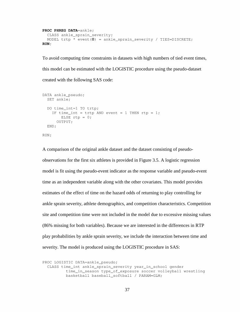
37
PROC PHREG DATA=ankle; CLASS ankle_sprain_severity; MODEL trtp * event(0) = ankle_sprain_severity / TIES=DISCRETE; RUN;
To avoid computing time constraints in datasets with high numbers of tied event times,
this model can be estimated with the LOGISTIC procedure using the pseudo-dataset
created with the following SAS code:
DATA ankle_pseudo; SET ankle; DO time_int=1 TO trtp; IF time_int = trtp AND event = 1 THEN rtp = 1; ELSE rtp = 0; OUTPUT; END; RUN;
A comparison of the original ankle dataset and the dataset consisting of pseudo-
observations for the first six athletes is provided in Figure 3.5. A logistic regression
model is fit using the pseudo-event indicator as the response variable and pseudo-event
time as an independent variable along with the other covariates. This model provides
estimates of the effect of time on the hazard odds of returning to play controlling for
ankle sprain severity, athlete demographics, and competition characteristics. Competition
site and competition time were not included in the model due to excessive missing values
(86% missing for both variables). Because we are interested in the differences in RTP
play probabilities by ankle sprain severity, we include the interaction between time and
severity. The model is produced using the LOGISTIC procedure in SAS:
PROC LOGISTIC DATA=ankle_pseudo; CLASS time_int ankle_sprain_severity year_in_school gender time_in_season type_of_exposure soccer volleyball wrestling basketball baseball_softball / PARAM=GLM;

38
MODEL rtp(DESC) = time_int ankle_sprain_severity time_int * ankle_sprain_severity year_in_school gender height_inches weight_pounds time_in_season type_of_exposure soccer volleyball wrestling basketball baseball_softball / LACKFIT; RUN;
All independent variables included in the CLASS statement will be treated as categorical.
The PARAM=GLM option in the CLASS statement overrides the default effect coding in
the design matrix and creates a set of indicator variables with the highest value of the
categorical variable as the reference. The DESCENDING option in the MODEL
statement will predict the probability of rtp=1 instead of rtp=0. The LACKFIT option in
the model statement provides the Hosmer and Lemeshow goodness of fit test for the
logistic regression model. The SAS output for this model is provided in Figure 3.6.
Notice in the Type 3 Analysis of Effects that the interaction between time and severity is
significant (p=.001). This means that the hazard odds of RTP varies for different time
intervals and levels of severity. The LSMEANS statement in PROC LOGISTIC can be
used to calculate hazard odds ratios for the different combinations of time and severity:
LSMEANS time_int * ankle_sprain_severity / PDIFF EXP CL;
The PDIFF option performs comparisons of LS Means, and the EXP and CL options
provide the hazard odds ratios and confidence limits for the different combinations of
time and severity.
3.4.4 Results
There were 2,086 documented new lateral ankle sprains among field and court sport
athletes with a known injury date. Of those, 1,305 (62.6%) were 1st degree sprains, 645
(30.9%) were 2nd degree sprains, and 136 (6.5%) were 3rd degree sprains. Of the new

39
lateral ankle sprains, 1,957 (94%) had a documented date for return to play; 129 (6%)
were censored cases of RTP. Since only new lateral ankle sprains were considered, the
number of injured athletes and the number of injuries were equal. A majority of the
injured athletes were male (64%) with 1st degree sprains (63%). The mean age of injured
athletes was 16 (SD=1); approximately one quarter of injured athletes were in each of the
high school grades (freshman, sophomore, junior, senior). Most injuries occurred in the
regular season (75%) during competition (53%). A summary of demographic, injury, and
competition characteristics is provided in Table 3.3.
Return to play probabilities, defined as the probability of returning to play during the
specified time interval, given that RTP did not occur prior to that time interval, are
presented by ankle sprain severity in Table 3.4. For 1st and 2nd degree lateral ankle
sprains, the probability of RTP is highest 10-21 days after injury. For 3rd degree lateral
ankle sprain, the probability of RTP is highest at least four weeks after injury. The log
rank test identified a significant difference in survival curves between ankle sprain
severity (p<.0001); there was a significant difference between 1st and 2nd degree survival
curves (p<.0001) and 1st and 3rd degree survival curves (p<.0001), but there was no
significant difference between 2nd and 3rd degree survival curves (p=.9). In the context of
the RTP event measured in discrete time, failure probabilities are of more interest than
survival probabilities. Failure for a specified time interval is the cumulative probability
that RTP occurs prior to that time interval. The significant difference in survival curves is
illustrated by plots of cumulative RTP probabilities in Figure 3.7.
The dependent variable of the discrete logistic regression model was coded so those who
experienced the RTP event were compared to those who did not RTP (Table 3.5). There
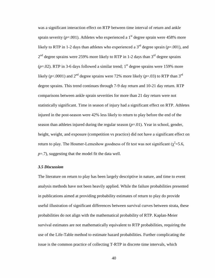
40
was a significant interaction effect on RTP between time interval of return and ankle
sprain severity (p=.001). Athletes who experienced a 1st degree sprain were 458% more
likely to RTP in 1-2 days than athletes who experienced a 3rd degree sprain (p=.001), and
2nd degree sprains were 259% more likely to RTP in 1-2 days than 3rd degree sprains
(p=.02). RTP in 3-6 days followed a similar trend; 1st degree sprains were 159% more
likely (p<.0001) and 2nd degree sprains were 72% more likely (p=.03) to RTP than 3rd
degree sprains. This trend continues through 7-9 day return and 10-21 day return. RTP
comparisons between ankle sprain severities for more than 21 day return were not
statistically significant. Time in season of injury had a significant effect on RTP. Athletes
injured in the post-season were 42% less likely to return to play before the end of the
season than athletes injured during the regular season (p=.01). Year in school, gender,
height, weight, and exposure (competition vs practice) did not have a significant effect on
return to play. The Hosmer-Lemeshow goodness of fit test was not significant (χ2=5.6,
p=.7), suggesting that the model fit the data well.
3.5 Discussion
The literature on return to play has been largely descriptive in nature, and time to event
analysis methods have not been heavily applied. While the failure probabilities presented
in publications aimed at providing probability estimates of return to play do provide
useful illustration of significant differences between survival curves between strata, these
probabilities do not align with the mathematical probability of RTP. Kaplan-Meier
survival estimates are not mathematically equivalent to RTP probabilities, requiring the
use of the Life-Table method to estimate hazard probabilities. Further complicating the
issue is the common practice of collecting T-RTP in discrete time intervals, which

41
requires time to event analysis techniques different than developing a Cox regression
model. This paper provides detailed guidance to assist athletic trainers and sports
medicine researchers with understanding the appropriate data structure required for time
to event analysis and the methodology appropriate for analyzing discrete time RTP
categories. Further, the programming statements and data example provide a detailed
description of how these models are run and how they can be interpreted. The data
example demonstrates how the life-table is useful for directly applicable information on
expected time to return to play, while the discrete logistic regression model for this
example highlights the relationship between severity and time to return to play.
3.5.1 Return to play probabilities by ankle sprain severity
Ankle sprain severity has a significant effect on estimated time to return to play. The
more severe the sprain, the longer it takes to RTP. After an injury is diagnosed, an
immediate discussion typically surrounds healing timelines and when the athlete will be
cleared to return to participation. The RTP probabilities from the life-table can help
athletes, coaches, and trainers determine reasonable expectations for return times based
on sprain severity. For a 1st degree sprain, athletes have roughly a 50% chance of
returning in about one week, but a much higher chance of returning in the third week
after injury. For a 2nd degree sprain, an athlete has the highest chance of RTP in the third
week after injury. A 3rd degree sprain would put an athlete returning at least four weeks
after injury. Regardless of sprain severity, an athlete has a fairly high chance of RTP
within one month. Equipping athletes with reasonable expectations regarding return times
can allow them adequate time to heal without rushing to return. Further, availability of

42
RTP probabilities can ease coaching decisions concerning lineups without the injured
player if an estimated return timeline is available.
3.5.2 Multivariate relationship between RTP, time and severity
Similar to the life-table finding that ankle sprain severity has an effect on T-RTP, the
discrete logistic regression model indicates a statistically significant interaction between
time and severity. The hazard odds of RTP within three weeks of injury are higher for 1st
and 2nd degree sprains compared to 3rd degree sprains. This finding is consistent with
more severe ankle sprains resulting in longer return times. Also of interest was the effect
of gender and exposure on RTP. While only a moderately significant effect, male athletes
were more likely to return during the season than females. Female athletes only
comprised one-third of the sample, which could impact this result. Although studies have
shown only minor gender differences in injury vulnerability [87, 88], there have been
recent opinion reports that gender plays a role in injury frequency and healing timelines
[45, 46]. Theories postulate that females are more vulnerable to injury, particularly ankle
sprains, due to higher estrogen levels, less powerful muscles, increased likelihood of
calcium and Vitamin D deficiency, and a wider pelvis resulting in a different alignment
of the knee and ankle [45, 46]. Examining gender differences in RTP timelines would
provide a significant contribution to the body of literature surrounding this issue. Injuries
occurring during competition were marginally less likely to result in RTP during the
season than injuries occurring during practice, perhaps indicating that competition
injuries are more severe than practice injuries. Players injured during the post-season
were significant less likely to RTP during the season than players injured during the
regular season. This is likely due to the end of the study period occurring in such close

43
proximity to post-season play. Perhaps only injuries that occur in the regular season
should be included in analysis to allow adequate time for follow up in future studies.
While only high school athletes were considered in this analysis, the sample was equally
representative of each of the four grade classifications. Year in school, and by extension,
age, did not have an effect on RTP. These findings confirm that for athletes, coaches, and
clinicians, ankle sprain severity should be the priority consideration when evaluating RTP
timeline decisions.
3.6 Conclusion
Return to play has typically been summarized in a descriptive manner and excluded
athletes with no follow up information regarding return. The application of time to event
analysis methods for discrete time have been applied to RTP using ankle sprain injuries
reported by high school athletes. These methods provide return time probabilities and
explore multivariate relationships between RTP and demographic and competition
characteristics while accounting for censored cases. The findings suggest that ankle
sprain severity has the strongest impact on RTP timelines. Historically, RTP estimations
have been based on anecdotal evidence and subjective opinion, but these can be
inaccurate and, coupled with pressure from coaches, athletes, and other external
influences, athletes can be cleared to RTP too early. Returning to play too soon can lead
to recurrent injury and long-term conditions such as osteoarthritis. In practice, all
evidence needs to be considered when making RTP decisions. The addition of evidence-
based, objective indicators in the form of RTP probabilities to this body of evidence can
provide more accurate estimates of return times and more confidence in returning an
athlete to play.

44
Table 3.1 Distribution functions for discrete time to return to play Let T be a discrete random variable that can take on values 𝒕𝒕𝒋𝒋, 𝒋𝒋 = 𝟏𝟏,𝟐𝟐, …, where 𝒕𝒕𝟏𝟏 < 𝒕𝒕𝟐𝟐 < ⋯. Function Formula Definition Probability mass function (pmf)
𝑜𝑜�𝑎𝑎𝑗𝑗� = 𝐼𝐼(𝑅𝑅𝑅𝑅𝑅𝑅𝐼𝐼 = 𝑎𝑎𝑗𝑗) probability that RTP took place at time 𝑎𝑎𝑗𝑗
Cumulative distribution function (cdf, or Failure)
𝐹𝐹(𝑎𝑎) = 𝐼𝐼(𝑅𝑅𝑅𝑅𝑅𝑅𝐼𝐼 < 𝑎𝑎) probability that RTP occurred prior to time 𝑎𝑎
Survival function 𝑆𝑆(𝑎𝑎) = 𝐼𝐼(𝑅𝑅𝑅𝑅𝑅𝑅𝐼𝐼 ≥ 𝑎𝑎) probability that RTP
occurred at time 𝑎𝑎 or later
Hazard function ℎ�𝑎𝑎𝑗𝑗� = 𝐼𝐼�𝑅𝑅𝑅𝑅𝑅𝑅𝐼𝐼 = 𝑎𝑎𝑗𝑗 � 𝑅𝑅𝑅𝑅𝑅𝑅𝐼𝐼 ≥ 𝑎𝑎𝑗𝑗) conditional probability
of RTP at time 𝑎𝑎𝑗𝑗 given the athlete has not returned to play prior to 𝑎𝑎𝑗𝑗
Cumulative hazard function
H(𝑎𝑎) = �ℎ�𝑎𝑎𝑗𝑗�𝑖𝑖𝑗𝑗≤𝑖𝑖
sum of hazard up to time 𝑎𝑎
Table 3.2 Estimated season start and end dates for field and court sports
Sport Season start date Season end date Football August 1 December 1
Fall soccer (boys/girls) August 1 November 15
Spring soccer (boys/girls) December 15 April 15
Volleyball August 1 November 15
Wrestling November 1 March 15
Basketball (boys/girls) November 1 March 15
Baseball/softball February 1 June 1

45
Table 3.3 Demographic, injury, and competition characteristics for high school athletes with new lateral ankle sprain (N=2,086) Variable n (%) Gender Male 1337 (64.1) Female 749 (35.9) Grade in school Freshman 450 (21.9) Sophomore 524 (25.4) Junior 535 (26.0) Senior 550 (26.7) Sport Football 752 (36.1) Boys fall soccer 127 (6.1) Girls fall soccer 144 (6.9) Volleyball 234 (11.2) Boys basketball 342 (16.4) Girls basketball 289 (13.8) Wrestling 73 (3.5) Baseball 43 (2.1) Softball 82 (3.9) Ankle sprain severity 1st degree 1305 (62.5) 2nd degree 645 (30.9) 3rd degree 136 (6.5) Returned to play Yes 1957 (93.8) No 129 (6.2) Time to return to play 1-2 days 293 (14.0) 3-6 days 659 (31.6) 7-9 days 421 (20.2) 10-21 days 504 (24.2) More than 21 days 209 (10.0) Time in season Preseason 458 (22.0) Regular season 1561 (74.9) Post season 64 (3.1)

46
Table 3.3 (continued) Demographic, injury, and competition characteristics for high school athletes with new lateral ankle sprain (N=2,086) Variable n (%) Type of exposure Competition 1113 (53.4) Practice 973 (46.6) Competition site Home 139 (47.6) Away 143 (49.0) Neutral 10 (3.4) Competition time Warm-up 6 (2.1) Beginning 47 (16.4) Middle 159 (55.4) End 73 (25.4) Overtime 2 (0.7)
Table 3.4 Estimated return to play probabilities by ankle sprain severity Ankle sprain severity Time interval 1st degree
P1 (95% CI) 2nd degree
P 1 (95% CI) 3rd degree
P 1 (95% CI) 1-2 days .17 (.15, .19) .10 (.08, .13) .03 (.00, .06) 3-6 days .42 (.39, .45) .30 (.27, .34) .21 (.14, .27) 7-9 days .43 (.39, .47) .32 (.27, .36) .23 (.15, .31) 10-21 days .71 (.66, .76) .72 (.67, .78) .53 (.42, .64) More than 21 days .56 (.44, .68) .72 (.61, .84) .79 (.64, .93) 1Probability of RTP during the time interval given that the athlete has not returned prior to that interval.

47
Table 3.5 Discrete time logistic regression of return to play on time, injury severity, athlete demographics, and competition characteristics for lateral ankle sprains in high school athletes (n=5,132) Variable Hazard
odds ratio 95% Confidence
interval for hazard odds ratio
p-value
Year in school Freshman vs Senior 0.89 (0.74, 1.09) .3 Sophomore vs Senior 0.87 (0.73, 1.04) .1 Junior vs Senior 0.93 (0.78, 1.12) .4 Gender Male vs Female 1.21 (0.98, 1.49) .1 Height (inches) 0.99 (0.97, 1.01) .4 Weight (inches) 1.00 (0.99, 1.00) .7 Time in season Pre-season vs regular season 1.08 (0.91, 1.28) .4 Post-season vs regular season 0.58 (0.40, 0.86) .01 Exposure Competition vs practice 0.87 (0.75, 1.00) .1 T-RTP * ankle sprain severity .001 1-2 day return 1st degree vs 3rd degree 5.58 (2.03, 15.31) .001 2nd degree vs 3rd degree 3.59 (1.28, 10.08) .02 3-6 day return 1st degree vs 3rd degree 2.59 (1.63, 4.12) <.0001 2nd degree vs 3rd degree 1.72 (1.06, 2.79) .03 7-9 day return 1st degree vs 3rd degree 2.45 (1.47, 4.07) .001 2nd degree vs 3rd degree 1.49 (0.88, 2.55) .1 10-21 day return 1st degree vs 3rd degree 2.11 (1.24, 3.60) .01 2nd degree vs 3rd degree 2.23 (1.28, 3.88) .005 more than 21 day return 1st degree vs 3rd degree 0.49 (0.21, 1.14) .1 2nd degree vs 3rd degree 0.98 (0.40, 2.40) .9 T-RTP=Time to return to play Note: Five indicators for sport were included in the model. Note: The main effects of both time interval and ankle sprain severity are not included in the table; they are included in a significant interaction and are not practically interpretable.
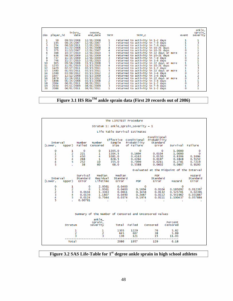
48
Figure 3.1 HS RioTM ankle sprain data (First 20 records out of 2086)
Figure 3.2 SAS Life-Table for 1st degree ankle sprain in high school athletes
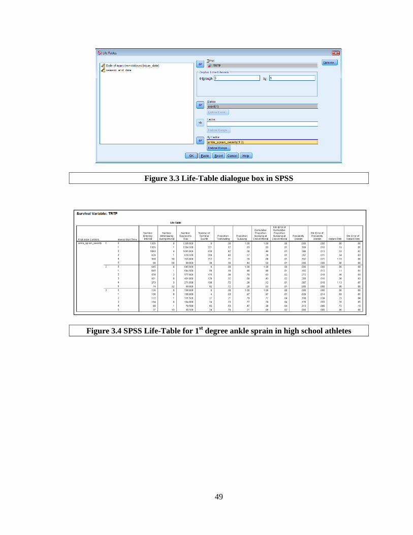
49
Figure 3.3 Life-Table dialogue box in SPSS
Figure 3.4 SPSS Life-Table for 1st degree ankle sprain in high school athletes
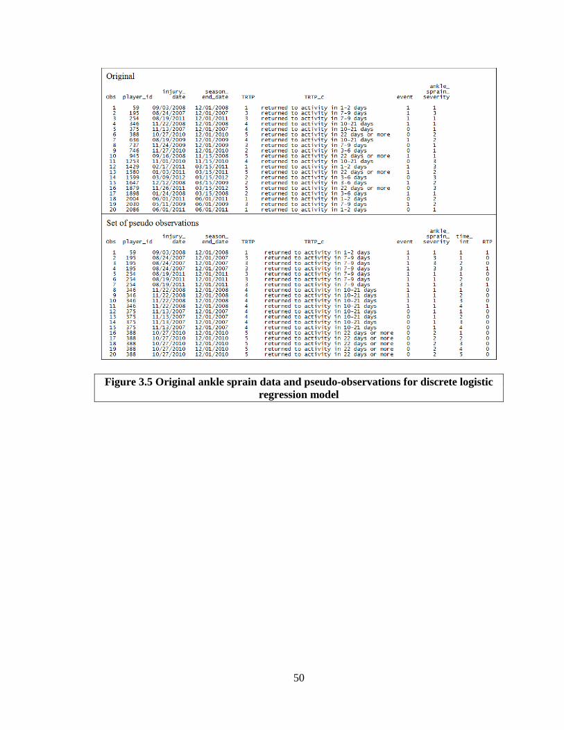
50
Figure 3.5 Original ankle sprain data and pseudo-observations for discrete logistic regression model

51
Figure 3.6 Maximum likelihood estimates of Discrete-Time Logistic Model for HS RioTM ankle sprain data
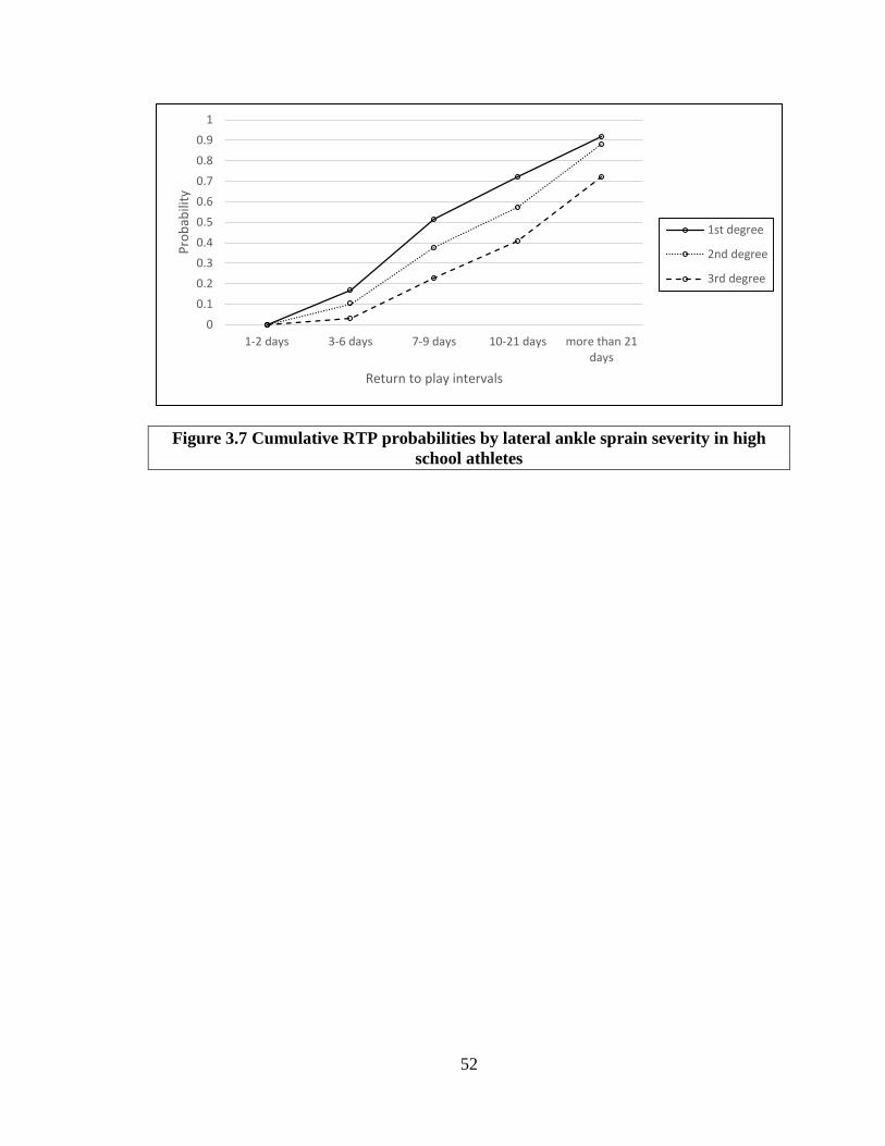
52
Figure 3.7 Cumulative RTP probabilities by lateral ankle sprain severity in high school athletes
00.10.20.30.40.50.60.70.80.9
1
1-2 days 3-6 days 7-9 days 10-21 days more than 21days
Prob
abili
ty
Return to play intervals
1st degree
2nd degree
3rd degree
53
4 Return to Play Probabilities after Knee Injury in High School Athletes
4.1 Introduction
Return to play (RTP) decisions have historically been determined using subjective
reasoning; therefore, there is a need for more objective methods to assist in the
determination of RTP to ensure athletes are not returning too soon. Typical research
studies involving RTP report rates or proportions, but these measures can be inaccurate in
instances where a lack of follow-up data excludes some athletes from analysis. Time to
event analysis is a commonly used statistical analysis method that can provide more
accurate estimates for time to return to play (T-RTP) by accounting for all injured
athletes regardless of lack of follow up concerning RTP. These analysis techniques have
not been heavily applied or related to RTP, and will provide athletic trainers, coaches,
team physicians, and other members of the sports medicine team more accurate means to
estimate return time. For prognosis, it is preferable to know the likelihood of an
individual experiencing the outcome of interest within a given timeframe as opposed to
summary results from cumulative risks and rates. In addition, it is likely that some
athletes will not experience a return to play event, indicating the presence of censored
cases. Time to event analysis can be applied to address both issues by generating
evidence-based, objective estimates of when an athlete is likely to return following a
given injury while accounting for censored cases. The accuracy of predicting T-RTP can
be improved using these techniques, resulting in better patient care through education,
improved coach-medical staff relations, and more efficient use of an athletic trainer’s
clinical time.
54
Knee joint ligament sprains are the second most common lower extremity (LE) sports-
related injury [2, 3, 65]. Medial collateral ligament (MCL) sprains are the most common
ligament injuries at the knee and occur frequently in football [66], ice hockey [67], soccer
[68], and skiing [69], all sports in which body movements causing high valgus stress at
the knee are common [70, 71]. Incidence of anterior cruciate ligament (ACL) injury has
recently risen significantly in adolescent athletes [7]. This rise could potentially be due to
improvements in identification of injury through diagnostic testing [1], or an increase in
participation in sports where the mechanisms of ACL injury are common. Basketball,
football, and soccer participation has increased among adolescent athletes; these sports
often require deceleration or change of direction forces [7]. Knee joint ligament sprains
lead to time lost from activity, functional and chronic instability, and joint degeneration
over time, even though surgery is not typical. For mild (Grade 1) MCL sprains, reported
diminished functional capacity lasts for several weeks with RTP ranging from 4 to 19
days post-injury [75]; reported diminished functional capacity for moderate (Grade 2)
MCL sprains ranges from 3 to 8 weeks [76]. ACL injury RTP guidelines suggest it could
take between 4 and 8 weeks for full range of motion to return and swelling to subside
[77]. As evidenced by these imprecise timeframes, healing and RTP timelines are
difficult to predict based on tissue damage alone.
The extent of tissue damage and tissue healing timelines are not direct indicators of how
long an athlete will be withheld from play, and many RTP decisions focus on resolution
of symptoms. However, symptom resolution and restoration of function can follow a
vastly different timeline than tissue healing, making a prognosis of time to RTP difficult.
Current RTP estimations are predominantly based on subjective reports of the individual

55
patient’s symptoms and anecdotal, expert opinion of clinicians. While neither approach is
incorrect, there is limited clinical epidemiological evidence to substantiate current RTP
predictions for knee injuries. As a consequence, athletes may have unrealistic
expectations for RTP, contributing to poor compliance with rehabilitation programs,
disregarding symptoms, and pushing for earlier RTP, putting them at risk of subsequent
or increasingly severe injury. Recurrent knee injuries can lead to concomitant long-term
health issues; ligament damage to the knee can result in early-onset post-traumatic
osteoarthritis (OA), most often within 10 to 20 years after initial injury [9, 10]. For high
school athletes suffering ankle or knee injuries, this indicates the potential for
degenerative conditions before age 30. Posttraumatic OA symptoms include joint pain,
swelling, limited motion, and disability [11]; these symptoms are associated with
decreased physical activity, obesity, cardiovascular disease, and depression stemming
from loss of function and disability due to injury to the affected joint [12, 13]. To address
the potential significant public health issues related to knee joint ligament sprains in the
adolescent athlete population, there is a need for the development of effective strategies
to diminish the impact of joint injuries, improve compliance to rehabilitation programs,
and reduce the risk of reinjury, with the goal of avoiding long-term effects from injury
and the continued maintenance of joint health. It is critical that athletic trainers,
physicians, and coaches be able to accurately gauge when an athlete is safe to return to
play. The purpose of this study was to analyze RTP probabilities between different
single-ligament knee injuries using time to event analysis methodologies.

56
4.2 Methods
4.2.1 Design and sample
This observational study consisted of a secondary data analysis of athlete injury data
from the High School RIOTM Injury Surveillance System (ISS) database. All US high
schools with a National Athletic Trainers’ Association (NATA) certified athletic trainer
(AT) were eligible for enrollment in this ISS; AT’s who enrolled their school completed
the online “Exposure Report Form” for reportable injuries each week. New single-
ligament knee sprains experienced by high school athletes from approximately 100 high
schools in the US during regularly scheduled participation in school-sanctioned sports for
seven academic years (2005-2006 through 2011-2012) were considered. Only field and
court sports (football, boys/girls soccer, volleyball, wrestling, basketball, baseball, and
softball) were included as these athletes were more likely to suffer knee injury due to the
nature of the sport. The use of the HS RIO TM ISS database for the purpose of evaluating
RTP probabilities was approved by the University Institutional Review Board.
Within the HS RIOTM ISS, a sprain was defined as injury to the ligamentous or capsular
tissue [2, 83]. All knee joint ligament sprains that required the athlete to be removed from
participation and diagnosed by the treating health care professional were reported,
regardless of time lost from participation. No unique personal identifying information
was contained in the dataset; the de-identification process of the data prohibited linking
multiple injuries on the same athlete allowing only new injuries to be considered for
analysis. A new injury was defined as a knee joint ligament sprain with an acute,
traumatic onset of symptoms with no prior history of that injury. The ligaments under
consideration include the anterior cruciate ligament (ACL), posterior cruciate ligament

57
(PCL), lateral collateral ligament (LCL), and medial collateral ligament (MCL) [89].
There were 1,049 documented new single-ligament knee injuries (classified under injury
type=“ligament sprain”) among field and court sport athletes with a known injury date.
RTP probabilities will be presented stratified by injured knee ligament.
4.2.2 Measures
Time to Return to Play Outcome. T-RTP was defined as the time between injury and
when the athlete was able to return to play. In the HS RIOTM ISS database, the number of
days the athlete was withheld from participation was collected in intervals of 1-2 days, 3-
6 days, 7-9 days, 10-21 days, and more than 21 days [83].
Censored Cases of Return to Play. Athletes who did not return to play after injury were
considered censored cases of RTP. A censored observation could have occurred in one of
six ways: 1) the athlete was determined to be medically disqualified for the season; 2) the
athlete was determined to be medically disqualified for their career; 3) the athlete chose
not to continue but was not medically disqualified; 4) the athlete was released from the
team but was not medically disqualified; 5) the athlete did not return for unspecified
reasons; or 6) the season ended before the athlete could return to play. In all cases,
censored observations were non-informative and right censored. To compute T-RTP
categories for censored cases, estimated season end dates for each sport were used as a
proxy for last date of contact. The number of days between injury date and season end
date was calculated, and each injury was then classified into the appropriate T-RTP
category. Estimated season start and end dates for each sport are listed in Table 4.1.

58
Athlete Demographics and Competition Characteristics. Demographic characteristics
were documented for each injured athlete including year in school (freshman, sophomore,
junior, senior), age in years, and gender. Competition characteristics at the time of injury
were also documented, including sport in which the athlete was participating, time in
season (preseason, regular season, postseason), type of exposure (competition or
practice), competition site (home, away, neutral site), and competition time (warm-ups,
beginning, middle, end, overtime). Indicators for sport (football, soccer, volleyball,
wrestling, basketball, baseball/softball) were included in the model to account for
differences in injury frequency among field and court sports that may influence RTP.
4.2.3 Data analysis
Data were summarized using descriptive statistics, including means and standard
deviations or frequency distributions. The Life-Table survival analysis method was used
to calculate return to play probability estimates stratified on injured knee ligament. The
log-rank test was used to determine differences in RTP probabilities between strata; the
Tukey adjustment for multiple comparisons was used for pairwise comparisons of RTP
probabilities between strata. Discrete logistic regression was used to estimate hazard odds
ratios for RTP due to the discrete nature of the T-RTP outcome; the Hosmer-Lemeshow
test was used to assess the fit of the discrete logistic regression model. Data analysis was
performed using SAS for Windows (version 9.4, SAS Institute, Inc., Cary NC, USA); an
alpha level of .05 was used throughout.
4.3 Results
Of all new single-ligament knee injuries, 310 (29.5%) were ACL sprains, 27 (2.6%) were
PCL sprains, 103 (9.8%) were LCL sprains, and 609 (58.1%) were MCL sprains. Of the

59
1,049 total knee joint ligament sprains, 721 (68.7%) had a documented date for return to
play; 328 (31.3%) were censored cases of RTP. Since only new knee sprains were
considered, the number of injured athletes and the number of injuries were equal. A
summary of demographic, injury, and competition characteristics is provided in Table
4.2. A majority of the injured athletes were male (80.3%) with MCL sprains (58.1%).
The mean age of injured athletes was 16 (SD=1); over half of the injured athletes were in
their junior or senior years. Most injuries occurred in the regular season (76.9%) during
competition (63.8%).
Return to play probabilities, defined as the probability of returning to play during the
specified time interval, given that RTP did not occur prior to that time interval, are
presented by injured knee ligament in Table 4.3. As expected, the probability of RTP for
ACL injuries was low, even three weeks after injury. For PCL sprain, the probability of
RTP increased from 0.2 at 3-6 days to 0.33 at 10-21 days to 0.5 four weeks after injury.
The probability of RTP after LCL and MCL sprains is approximately 0.5 at 10-21 days
after injury. The log rank test identified a significant difference in survival curves
between injured knee ligaments (p<.0001); pairwise comparisons between ligaments
resulted in significant differences for all comparisons (p<.0001 for all). In the context of
the RTP event measured in discrete time, failure probabilities are of more interest than
survival probabilities. Failure for a specified time interval is the cumulative probability
that RTP occurs prior to that time interval. The significant difference in survival curves is
illustrated by plots of cumulative RTP probabilities in Figure 4.1.
The dependent variable of the discrete logistic regression model was coded so those who
experienced the RTP event were compared to those who did not RTP (Table 4.4). There

60
was a significant interaction effect on RTP between time interval of return and injured
knee ligament (p=.01). Athletes who experienced ACL sprain were 78% less likely to
RTP in 1-2 days than athletes with MCL sprain (p=.002), 81% less likely to return in 3-6
days (p<.0001), 91% less likely to return in 7-21 days (p<.0001), and 74% less likely to
return 4 weeks after injury (p<.0001). Athletes who experienced LCL sprains were 213%
more likely to return in 1-2 days than athletes with MCL sprain (p=.02), 73% more likely
to return in 3-6 days (p=.04), and 103% more likely to return in 7-9 days (p=.02). PCL
sprains were not included in the discrete logistic model due to the relatively small number
(3%) of athletes who reported this injury; this small sample size led to inflated standard
errors and unstable estimates. Type of exposure had a significant effect on RTP; athletes
suffering a single-ligament knee sprain during competition were 25% less likely to RTP
before the end of the season than athletes injured during practice (p=.01). Year in school,
gender, and time in season did not have a significant effect on RTP. The Hosmer-
Lemeshow goodness of fit test was not significant (χ2=7.45, p=.5), suggesting that the
model fit the data well.
4.4 Discussion
As expected, MCL and ACL sprains were the most common occurring knee injuries
among the high school athletes, and athletes who suffered an ACL injury had
significantly lower RTP probabilities than other knee ligament injuries. After an injury is
diagnosed, an immediate discussion typically surrounds healing timelines and when the
athlete will be cleared to return to participation. The RTP probabilities from the life-table
can help athletes, coaches, and athletic trainers determine reasonable expectations for
return times based on injured knee ligament. Athletes injuring the ACL any time during
61
the season have only a 1 in 3 chance of returning before the end of the season. This
finding is consistent with 4 to 8 week estimates from existing RTP guidelines given the
study period defined by sport seasons [77]. Those suffering PCL sprain have a 50%
chance of returning before season end. Athletes with LCL and MCL sprains have roughly
a 50% chance of returning in the third week after injury, which is also consistent with
existing RTP estimations [75]. Regardless of the knee ligament injured, athletes have a
very small chance of RTP within two weeks of injury; RTP probabilities increase slightly
for PCL, LCL and MCL injuries after two weeks. Equipping athletes with reasonable
expectations regarding return times can allow them adequate time to heal without rushing
to return. In addition to an individual athlete’s clinical symptoms, availability of RTP
probabilities can ease coaching decisions concerning lineups without the injured player if
an estimated return timeline is available.
Similar to the life-table finding that injured knee joint ligament has an effect on T-RTP,
the discrete logistic regression model indicates a statistically significant interaction
between time and injured ligament. The hazard odds of RTP for ACL sprain are
significantly lower across all time points than MCL sprain. This finding is consistent with
longer healing times for ACL injury than other knee ligaments [77]. Conversely, the
hazard odds of RTP for LCL sprain are significantly higher the first week after injury
than MCL sprain. Also of interest was the significant effect of exposure on RTP. Players
injured during competition were less likely to return during the season than players
injured in practice, suggesting that competition injuries are more severe and require
longer healing times than practice injuries. No measure of injury severity for knee sprain
was available in the HS RIOTM database, and would have the potential for unreliability as

62
this is a subjective measure when assessed immediately following injury by an athletic
trainer. However, severity of injury should certainly be considered as a factor with the
potential to influence T-RTP. Timing in season likely did not have an effect on RTP as
most injuries across all ligaments occurred during the regular season. At least two-thirds
of knee joint ligament sprains were suffered by male athletes, a result likely due to the
high number of football players experiencing knee joint ligament sprains and consistent
with the literature [7]. Interestingly, while female basketball players suffered more ACL
and PCL injuries than male basketball players, gender did not have an effect on RTP.
This result held even after limiting the model to ACL sprains in basketball players (p=.2).
This finding seems to suggest that although girls are more vulnerable to ACL injury [7,
40], RTP timelines are not different than boys. Further research is necessary to explore
why girls are more susceptible to ACL injury and whether these risk factors have an
effect on T-RTP. Regardless of slightly more knee sprains in junior and senior athletes,
year in school, and by extension, age, did not have an effect on RTP.
Over 60% of knee ligament injuries were reported in football players. A sub-analysis of
football injuries was conducted; a discrete logistic regression model was fit exploring the
interaction between T-RTP and injured ligament controlling for year in school, time in
season, and exposure (Table 5.4). The Hosmer-Lemeshow goodness of fit test was not
significant (χ2=7.41, p=.5), suggesting that the model fit the data well. Findings were
similar in direction of the hazard odds ratios and significance to findings across all sports
with three exceptions. While year in school did not have an effect on RTP across all
sports, freshman football players were significantly less likely to RTP before the end of
the season after single-ligament knee sprain than senior football players (p=.02). Contrary
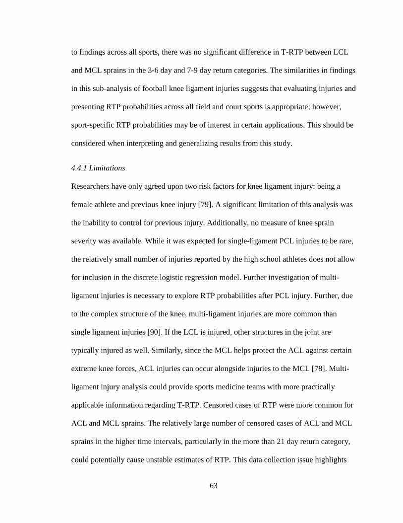
63
to findings across all sports, there was no significant difference in T-RTP between LCL
and MCL sprains in the 3-6 day and 7-9 day return categories. The similarities in findings
in this sub-analysis of football knee ligament injuries suggests that evaluating injuries and
presenting RTP probabilities across all field and court sports is appropriate; however,
sport-specific RTP probabilities may be of interest in certain applications. This should be
considered when interpreting and generalizing results from this study.
4.4.1 Limitations
Researchers have only agreed upon two risk factors for knee ligament injury: being a
female athlete and previous knee injury [79]. A significant limitation of this analysis was
the inability to control for previous injury. Additionally, no measure of knee sprain
severity was available. While it was expected for single-ligament PCL injuries to be rare,
the relatively small number of injuries reported by the high school athletes does not allow
for inclusion in the discrete logistic regression model. Further investigation of multi-
ligament injuries is necessary to explore RTP probabilities after PCL injury. Further, due
to the complex structure of the knee, multi-ligament injuries are more common than
single ligament injuries [90]. If the LCL is injured, other structures in the joint are
typically injured as well. Similarly, since the MCL helps protect the ACL against certain
extreme knee forces, ACL injuries can occur alongside injuries to the MCL [78]. Multi-
ligament injury analysis could provide sports medicine teams with more practically
applicable information regarding T-RTP. Censored cases of RTP were more common for
ACL and MCL sprains. The relatively large number of censored cases of ACL and MCL
sprains in the higher time intervals, particularly in the more than 21 day return category,
could potentially cause unstable estimates of RTP. This data collection issue highlights

64
the need for accurate RTP reporting. While the categorical collection of T-RTP on the
Exposure Report Form is common in sports injury surveillance, it would be more
efficient for investigation of RTP to collect exact return dates and allow for the precise
calculation of T-RTP probability estimates using Cox regression models. This is
particularly of concern for injuries that have healing timelines longer than three weeks,
which is typically the largest time point in the categorical collection of RTP.
4.5 Conclusion
Return to play has typically been summarized in a descriptive manner and excluded
athletes with no follow up information regarding return. The application of time to event
analysis methods for discrete time have been applied to RTP using single-ligament knee
sprain injuries reported by high school athletes. These methods provide return time
probabilities and explore multivariate relationships between RTP and demographic and
competition characteristics while accounting for censored cases. The findings suggest
that injured knee ligament has a strong impact on RTP timelines. As expected, ACL
injuries had the highest proportion of censored cases, and the least likelihood to RTP at
all time points following injury. The likelihood of RTP following MCL or LCL injuries
was far higher than that of the cruciate ligaments. Historically RTP estimations have been
based on anecdotal evidence and subjective opinion, but these can be inaccurate and,
coupled with pressure from coaches, athletes, and other external influences, athletes can
be cleared to RTP too early. Returning to play too soon can lead to recurrent injury and
the potential for long-term degenerative conditions. In practice, all evidence needs to be
considered when making RTP decisions. The addition of evidence-based, objective
indicators in the form of RTP probabilities to this body of evidence can provide the sports

65
medicine team with tools to determine more accurate estimates of return times and more
confidence in returning an athlete to play.

66
Table 4.1 Estimated season start and end dates for field and court sports
Sport Season start date Season end date Football August 1 December 1
Fall soccer (boys/girls) August 1 November 15
Spring soccer (boys/girls) December 15 April 15
Volleyball August 1 November 15
Wrestling November 1 March 15
Basketball (boys/girls) November 1 March 15
Baseball/softball February 1 June 1

67
Table 4.2 Demographic, injury, and competition characteristics for high school athletes with new single-ligament knee sprain by injured ligament (N=1,049) Injured knee ligament Variable ACL
(n=310) n (%)
PCL (n=27) n (%)
LCL (n=103) n (%)
MCL (n=609) n (%)
Gender Male 206 (66.5) 17 (63.0) 79 (76.7) 540 (88.7) Female 104 (33.5) 10 (37.0) 24 (23.3) 69 (11.3) Grade in school Freshman 48 (15.6) 3 (11.1) 27 (26.5) 110 (18.2) Sophomore 63 (20.4) 4 (14.8) 17 (16.7) 144 (23.8) Junior 109 (35.4) 11 (40.8) 24 (23.5) 160 (26.5) Senior 88 (28.6) 9 (33.3) 34 (33.3) 190 (31.5) Sport Football 156 (50.3) 10 (37.1) 55 (53.4) 420 (69.0) Boys fall soccer 19 (6.1) 2 (7.4) 9 (8.8) 26 (4.3) Girls fall soccer 24 (7.7) 2 (7.4) 7 (6.8) 25 (4.1) Volleyball 15 (4.8) 0 (0.0) 7 (6.8) 5 (0.8) Boys basketball 16 (5.2) 1 (3.7) 2 (1.9) 28 (4.6) Girls basketball 53 (17.1) 5 (18.5) 10(9.7) 24 (3.9) Wrestling 12 (3.9) 3 (11.1) 13 (12.6) 59 (9.7) Baseball 3 (1.0) 1 (3.7) 0 (0.0) 7 (1.1) Softball 12 (3.9) 3 (11.1) 0 (0.0) 15 (2.5) Returned to play Yes 97 (31.3) 19 (70.4) 91 (88.4) 514 (84.4) No 213 (68.7) 8 (29.6) 12 (11.6) 95 (15.6) Time to return to play 1-2 days 6 (1.9) 2 (7.4) 14 (13.6) 46 (7.6) 3-6 days 16 (5.2) 5 (18.5) 28 (27.1) 127 (20.8) 7-9 days 7 (2.3) 2 (7.4) 19 (18.5) 85 (13.9) 10-21 days 25 (8.0) 6 (22.2) 23 (22.3) 182 (30.0) More than 21 days 256 (82.6) 12 (44.5) 19 (18.5) 169 (27.7) Time in season Preseason 57 (18.4) 3 (11.1) 24 (23.3) 117 (19.2) Regular season 239 (77.1) 22 (81.5) 75 (72.8) 471 (77.3) Post season 14 (4.5) 2 (7.4) 4 (3.9) 21 (3.5) ACL=Anterior cruciate ligament; PCL=Posterior cruciate ligament; LCL=lateral collateral ligament; MCL=medial collateral ligament

68
Table 4.2 (continued) Demographic, injury, and competition characteristics for high school athletes with new single-ligament knee sprain by injured ligament (N=1,049) Injured knee ligament Variable ACL
(n=310) n (%)
PCL (n=27) n (%)
LCL (n=103) n (%)
MCL (n=609) n (%)
Type of exposure Competition 222 (71.6) 15 (55.6) 64 (62.1) 368 (60.4) Practice 88 (28.4) 12 (44.4) 39 (37.9) 241 (39.6) Competition site Home 33 (61.1) 0 (0.0) 3 (27.3) 37 (43.5) Away 20 (37.0) 3 (100.0) 8 (72.7) 41 (48.2) Neutral 1 (1.9) 0 (0.0) 0 (0.0) 7 (8.3) Competition time Warm-up 2 (3.8) 0 (0.0) 0 (0.0) 0 (0.0) Beginning 7 (13.2) 0 (0.0) 0 (0.0) 11 (12.9) Middle 29 (54.7) 3 (100.0) 7 (70.0) 43 (50.6) End 15 (28.3) 0 (0.0) 3 (30.0) 31 (36.5) Overtime 0 (0.0) 0 (0.0) 0 (0.0) 0 (0.0) ACL=Anterior cruciate ligament; PCL=Posterior cruciate ligament; LCL=lateral collateral ligament; MCL=medial collateral ligament

69
Table 4.3 Estimated return to play probabilities by injured knee ligament Injured knee ligament Time interval ACL
P1 (95% CI) PCL
P 1 (95% CI) LCL
P 1 (95% CI) MCL
P 1 (95% CI) 1-2 days .02 (.00, .03) .07 (.00, .17) .14 (.07, .20) .07 (.05, .09) 3-6 days .05 (.03, .07) .20 (.04, .36) .31 (.22, .41) .23 (.19, .26) 7-9 days .02 (.00, .04) .10 (.00, .23) .31 (.20, .43) .20 (.16, .23) 10-21 days .08 (.05, .11) .33 (.12, .55) .53 (.38, .68) .50 (.45, .56) More than 21 days .32 (.25, .40) .50 (.15, .85) .59 (.33, .85) .65 (.57, .74) 1Probability of RTP during the time interval given that the athlete has not returned prior to that interval. ACL=Anterior cruciate ligament; PCL=Posterior cruciate ligament; LCL=lateral collateral ligament; MCL=medial collateral ligament

70
Table 4.4 Discrete time logistic regression of return to play on time, injured knee ligament, athlete demographics, and competition characteristics for new single-ligament knee sprains in high school athletes (n=3,852) Variable Hazard
odds ratio 95% Confidence
interval for hazard odds ratio
p-value
Year in school Freshman vs Senior 0.83 (0.63, 1.09) .2 Sophomore vs Senior 1.07 (0.83, 1.37) .6 Junior vs Senior 1.02 (0.80, 1.28) .9 Gender Male vs Female 1.01 (0.69, 1.49) .9 Time in season Pre-season vs regular season 1.05 (0.81, 1.36) .7 Post-season vs regular season 0.69 (0.41, 1.16) .2 Exposure Competition vs practice 0.75 (0.60, 0.93) .01 T-RTP * injured knee ligament .01 1-2 day return ACL vs MCL 0.22 (0.09, 0.57) .002 LCL vs MCL 2.13 (1.12, 4.06) .02 3-6 day return ACL vs MCL 0.19 (0.11, 0.33) <.0001 LCL vs MCL 1.73 (1.05, 2.84) .03 7-9 day return ACL vs MCL 0.09 (0.04, 0.21) <.0001 LCL vs MCL 2.03 (1.12, 3.70) .02 10-21 day return ACL vs MCL 0.09 (0.05, 0.14) <.0001 LCL vs MCL 1.10 (0.57, 2.12) .8 more than 21 day return ACL vs MCL 0.26 (0.17, 0.41) <.0001 LCL vs MCL 0.82 (0.31, 2.15) .7 T-RTP=Time to return to play; ACL=Anterior cruciate ligament; PCL=Posterior cruciate ligament; LCL=lateral collateral ligament; MCL=medial collateral ligament Note: Five indicators for sport were included in the model. Note: PCL sprains were not included in the model; the relatively small sample size (n=27) resulted in inflated standard errors and unstable estimates. Note: The main effects of both time interval and injured knee ligament are not included in the table; they are included in a significant interaction and are not practically interpretable.
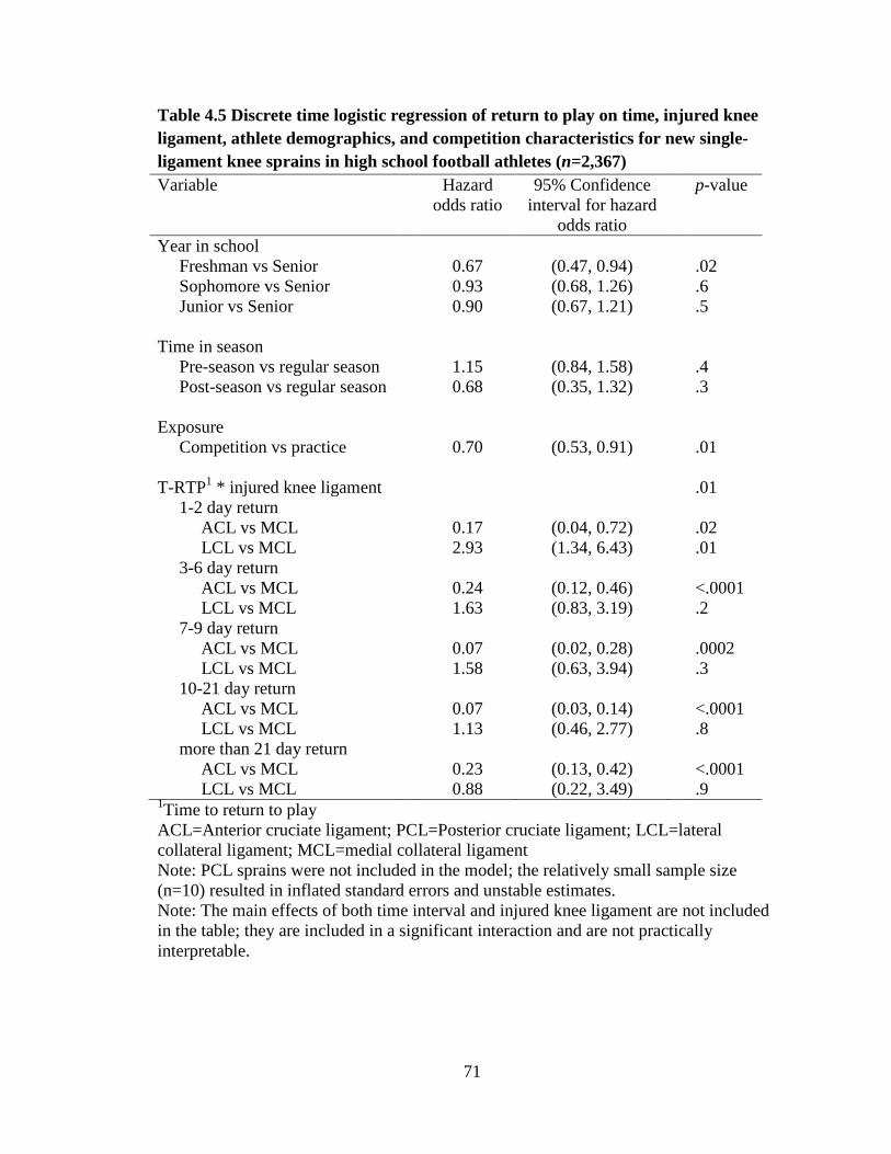
71
Table 4.5 Discrete time logistic regression of return to play on time, injured knee ligament, athlete demographics, and competition characteristics for new single-ligament knee sprains in high school football athletes (n=2,367) Variable Hazard
odds ratio 95% Confidence
interval for hazard odds ratio
p-value
Year in school Freshman vs Senior 0.67 (0.47, 0.94) .02 Sophomore vs Senior 0.93 (0.68, 1.26) .6 Junior vs Senior 0.90 (0.67, 1.21) .5 Time in season Pre-season vs regular season 1.15 (0.84, 1.58) .4 Post-season vs regular season 0.68 (0.35, 1.32) .3 Exposure Competition vs practice 0.70 (0.53, 0.91) .01 T-RTP1 * injured knee ligament .01 1-2 day return ACL vs MCL 0.17 (0.04, 0.72) .02 LCL vs MCL 2.93 (1.34, 6.43) .01 3-6 day return ACL vs MCL 0.24 (0.12, 0.46) <.0001 LCL vs MCL 1.63 (0.83, 3.19) .2 7-9 day return ACL vs MCL 0.07 (0.02, 0.28) .0002 LCL vs MCL 1.58 (0.63, 3.94) .3 10-21 day return ACL vs MCL 0.07 (0.03, 0.14) <.0001 LCL vs MCL 1.13 (0.46, 2.77) .8 more than 21 day return ACL vs MCL 0.23 (0.13, 0.42) <.0001 LCL vs MCL 0.88 (0.22, 3.49) .9 1Time to return to play ACL=Anterior cruciate ligament; PCL=Posterior cruciate ligament; LCL=lateral collateral ligament; MCL=medial collateral ligament Note: PCL sprains were not included in the model; the relatively small sample size (n=10) resulted in inflated standard errors and unstable estimates. Note: The main effects of both time interval and injured knee ligament are not included in the table; they are included in a significant interaction and are not practically interpretable.
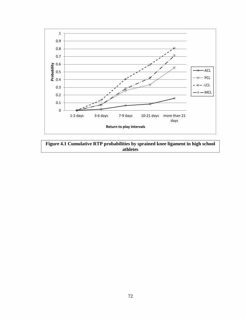
72
Figure 4.1 Cumulative RTP probabilities by sprained knee ligament in high school athletes
0
0.1
0.2
0.3
0.4
0.5
0.6
0.7
0.8
0.9
1
1-2 days 3-6 days 7-9 days 10-21 days more than 21days
Prob
abili
ty
Return to play intervals
ACL
PCL
LCL
MCL

73
5 Discussion and Conclusions
5.1 Summary
With approximately 30 million youth between the ages of 5 and 18 years in the US
participating in organized sports [7], there is high potential for young athletes to suffer
acute sports-related injuries or overuse injuries. It is estimated that 38% of high school
athletes will suffer sports-related injuries requiring treatment by a physician [7]; however,
actual percentages may be higher due to underreporting or failure to seek treatment [14].
Ankle ligament sprains are the most common injury across field and court sports [1, 8],
and incidence rates have been shown to be higher in adolescents than adults [51]. Knee
sprains are the second most common LE sports-related injury [2, 3, 65]. MCL sprains are
the most common ligament injury at the knee, and ACL injuries have recently risen
significantly in college and adolescent athletes [1, 7, 70, 71].
After injury, the athlete, coaches, and sports medicine team work together to formulate a
RTP plan. There is a high degree of variability among clinicians regarding factors
considered for RTP [15], resulting in a call to develop a more objective method to
determine when it is safe for an athlete to resume participation after injury. A three-step
decision making process has been proposed that recommends the evaluation of health
status, participation risk, and consideration of the influence of outside factors surrounding
the athlete [16]. The validation of this process illustrates the need for more objective
methods to evaluate the risk of return to play after injury. Extensive documentation of
risk factors for sports-related lateral ankle sprain and knee ligament injury exists in the
literature; however, there is little agreement among researchers on factors that affect

74
RTP. One thing that has been agreed upon, however, is that premature RTP is a
predisposing factor for subsequent injury [8]. Recurrent knee and ankle injuries can lead
to concomitant long-term degenerative joint diseases. Ligament damage to the ankle or
knee could potentially result in early-onset, post-traumatic OA, most often within 10 to
20 years after initial injury [9, 10]. For high school athletes suffering ankle or knee
injuries, this indicates they could suffer degenerative conditions before the age of 30.
Posttraumatic OA is typically reported in younger patients, and is significantly associated
with decreased physical activity, obesity, cardiovascular disease, and depression
stemming from loss of function and disability due to injury to the affected joint [12, 13].
This potentially significant public health issue related to ankle and knee sprains
necessitates the need for development of effective strategies to diminish the impact of
joint injuries, improve compliance with rehabilitation programs, and reduce the risk of
subsequent injury, with the goal of avoiding long-term effects from injury and the
continued maintenance of joint health.
Time to event analysis is a method of generating evidence-based, objective estimates of
when an athlete is likely to RTP following a given injury. The accuracy of predicting T-
RTP after ankle and knee sprains can be improved using time to event techniques,
resulting in better patient care through education, improved coach-medical staff relations,
and more efficient use of athletic trainer’s clinical time. Further, these analyses can
improve clinical decision-making by adding research-based evidence and also
incorporating the prognosis aspect to educate the patient and coaches about return to play
timelines. Detailed guidance has been provided to assist athletic trainers and sports
medicine researchers with understanding the appropriate data structure and programming
75
statements required for T-RTP analysis and the methodology appropriate for analyzing
discrete time RTP categories.
For 1st and 2nd degree lateral ankle sprains, the probability of RTP is highest 10-21 days
after injury. For 3rd degree lateral ankle sprain, the probability of RTP is highest at least
four weeks after injury. There was a significant interaction effect on RTP between time
interval of return and ankle sprain severity (p=.001). Athletes who experienced a 1st
degree sprain were 458% more likely to RTP in 1-2 days than athletes who experienced a
3rd degree sprain (p=.001), and 2nd degree sprains were 259% more likely to RTP in 1-2
days than 3rd degree sprains (p=.02). RTP in 3-6 days followed a similar trend; 1st degree
sprains were 159% more likely (p<.0001) and 2nd degree sprains were 72% more likely
(p=.03) to RTP than 3rd degree sprains. This trend continues through 7-9 day return and
10-21 day return. RTP comparisons between ankle sprain severities for more than 21 day
return were not statistically significant. Time in season had a significant effect on RTP;
athletes injured in the post-season were 42% less likely to return to play before the end of
the season than athletes injured during the regular season (p=.01). Gender had a marginal
effect on RTP (p=.1); male athletes were 21% more likely to return to play than female
athletes. Year in school, height, weight, and exposure (competition vs practice) did not
have a significant effect on return to play.
As expected, the probability of RTP for ACL injuries was low, even three weeks after
injury. For PCL sprain, the probability of RTP increased from 0.2 at 3-6 days to 0.33 at
10-21 days to 0.5 four weeks after injury. The probability of RTP after LCL and MCL
sprains is approximately 0.5 at 10-21 days after injury. There was a significant interaction
effect on RTP between time interval of return and injured knee ligament (p=.01). Athletes

76
who experienced ACL sprain were 78% less likely to RTP in 1-2 days than athletes with
MCL sprain (p=.002), 81% less likely to return in 3-6 days (p<.0001), 91% less likely to
return in 7-21 days (p<.0001), and 74% less likely to return 4 weeks after injury
(p<.0001). Athletes who experienced LCL sprains were 213% more likely to return in 1-2
days than athletes with MCL sprain (p=.02), 73% more likely to return in 3-6 days
(p=.04), and 103% more likely to return in 7-9 days (p=.02). PCL sprains were not
included in the discrete logistic model due to the relatively small number (3%) of athletes
who reported this injury; this small sample size led to inflated standard errors and
unstable estimates. Type of exposure had a significant effect on RTP; athletes suffering a
single-ligament knee sprain during competition were 25% less likely to RTP before the
end of the season than athletes injured during practice (p=.01). Year in school, gender,
and time in season did not have a significant effect on RTP. In a subset analysis of ACL
injuries in basketball players, gender still had no significant effect on RTP (p=.2).
The findings in this study provide a valuable start to addressing one component of the
incredibly complex RTP question. Incorporating these RTP probability estimates into the
participation risk component of a decision-based RTP model will provide stronger
guidance for RTP decision, leading to better patient care, a reduction in reinjury rates,
and a decrease in prevalence of early-onset OA among athletes.
5.2 Implications
The ability to return to play has long been a pivotal question posed by athletes and
coaches after injury, and few prognostic indicators have been explored to indicate when
RTP will occur. Clinicians have relied on their personal experience to predict when an
athlete might return, and RTP decisions vary tremendously between clinicians [15].

77
Coaches are left with little information to formulate coaching decisions such as line-ups
and substitutions. Further, this can potentially contribute to poor compliance with
rehabilitation programs due to athletes pushing for earlier RTP, which can lead to
subsequent or increasingly severe injuries [8]. A further consequence is the potential for
concomitant long-term health issues such as OA [9, 91]. The estimates of T-RTP
probabilities presented here contribute to the development of evidence-based, objective
strategies to determine when it is safe for an athlete to RTP. Avoiding premature RTP can
help diminish the impact of joint injuries, improve compliance with rehabilitation
programs, and reduce the risk of reinjury, with the goal of avoiding long-term effects
from injury and the continued maintenance of joint health.
5.3 Strengths and limitations
Alternative methods of reporting prognostic information exist, but a lack of certain
elements limit their application. The advantage of time to event analyses is through the
inclusion of censored cases, in other words, the inclusion within the analysis of those who
are still waiting to experience the event of interest during the study timeframe. Specific to
RTP, these analyses include data on athletes who do not return before the season is over,
thereby limiting the bias associated with these analyses. In contrast, the reporting of
proportions (e.g., 8/10 athletes returned after 3 days) eliminates data by not including
those who did not return. Similarly, reporting the average timeframe for return also
eliminates censored cases and may provide misleading information. This underestimation
is illustrated with lateral ankle sprain data in high school athletes in Table 5.1. The
estimated epidemiological incidence proportion (IP) is defined as the proportion of
injured athletes that RTP during a specified time interval out of the number of injured

78
athletes that have not yet returned to play at the beginning of the interval [27]. When the
number of censored cases is small, the IP and Lifetable RTP probabilities are nearly
identical. However, as the number of censored cases increases, the IP is smaller than the
Lifetable RTP probabilities. For 1st degree LAS, 5% of injuries were censored. Excluding
censored cases, it is estimated that 33% of athletes will return 22 or more days after
injury; however, accounting for censored cases, athletes with 1st degree LAS have an
estimated 56% chance of return 22 or more days after injury. This underestimation is
clear in LAS where only 6% of cases are censored; the differences would be even greater
in the presence of a higher proportion of censored cases. More than 30% of single-
ligament knee sprains in high school athletes were censored. Reporting proportions of
RTP for knee sprains will significantly underestimate T-RTP; probability estimates
determined using time to event analysis methods will be much more accurate in
estimating T-RTP for knee ligament injuries. The literature on return to play has been
largely descriptive in nature, and time to event analysis methods have only recently been
applied to T-RTP [32, 92]. While the failure probabilities based on Kaplan-Meier
survival estimates presented in these publications do provide useful illustration of
significant differences between RTP survival curves between strata, these probabilities
are not equivalent to the mathematical probability of RTP. The Life-Table method
detailed and utilized in this study is more appropriate in this setting as it allows the direct
computation of hazard probability estimates, which are equivalent to the probability of
RTP during a specified time interval given the injured athlete has not returned prior to the
specified time interval [31].

79
Participation in certain sports has been identified as a risk factor for injury [7, 8, 51, 61,
66-69]. To control for the observed differences in injury risk between types of sports, the
decision was made to restrict analyses to only field and court sports in this study. Further,
an indicator for sport was included in the discrete logistic regression models to control for
differences in RTP between sports. Football and basketball dominated ankle and knee
injury rates; girls basketball had higher incidence rates for single-ligament knee sprains
than boys basketball. Sub-analyses were conducted to determine whether it was
appropriate to report RTP probabilities and hazard odds ratios across all field and court
sports. Findings from these sub-analyses did not indicate that T-RTP results were
different enough to warrant stratification on sport at this time. There are certain
applications in which sport-specific RTP probabilities may be of interest; this should be
considered when interpreting and generalizing results from this study.
The HS RIOTM ISS has been established as a tracking system to determine incidence rates
of injuries in the high school athlete population, as well as provide a mechanism by
which to investigate risk factors for injury with the goal of reducing injury rates in high
school athletes to the lowest possible level while still encouraging participation in
organized sports [83]. NATA certified ATs volunteer to participate as reporters, and are
then categorized into 8 sampling strata by geographic location and high school size.
Schools from each substrata are randomly selected until a sample of 100 schools are
identified. If an AT drops from participation, their school will be replaced by another
school within the substrata. Participating ATs are offered $300-$400 depending on the
number of sports in which they report data and individualized injury reports following the
study’s conclusion [83]. While this sampling methodology is useful in maintaining a

80
nationally representative sample, the incentive to participate has the potential to bias
results based on these data. Of particular concern is the potential for surveillance bias,
which can result in an overestimation of the number of injuries in the ISS [93]. ATs may
be inclined to identify an injury that would otherwise not be reported, particularly those
with mild severity.
While the HS RIOTM ISS is useful for identifying risk factors for injury, documentation
is lacking for factors that may influence RTP. Patient demographics, symptoms, and
clinical injury evaluation information are well documented, but participation risk and
decision modifiers identified for consideration in the three-step decision based RTP
model are not collected on the exposure report form [16, 83]. In the analyses presented
here, prior injury information was not available for examination. A proxy for injury
severity for lateral ankle sprain was incorporated into the analyses; however, this was not
feasible for knee ligament injuries. Information on injury protection (i.e., use of taping or
bracing) after diagnosis was not reported. It is assumed that injuries reported to the HS
RIOTM ISS are not verified after diagnostic testing or more confirmatory diagnoses
methods by a clinician. This could potentially bias injury rates to ankle and knee
ligaments as specific injured ligaments could be missed by ATs on the field, or ligaments
could be identified as injured when they weren’t. Competition site (home, away, neutral
site) and competition time (warm-ups, beginning, middle, end, overtime) were not
included in analyses due to an abundance of missing data (86% missing for both). These
competition characteristics were not identified as potential factors affecting T-RTP, so
their exclusion is not of particular concern. However, it would be an addition to the body
of knowledge surrounding T-RTP to explore the effect of these characteristics further.

81
More accurate reporting of competition site and time is suggested for future injury
surveillance. Missing data for other study variables did not exceed 10%, eliminating the
need to account for missing data in analyses.
A significant limitation to the use of HS RIOTM data for evaluating T-RTP after ankle and
knee injury is that it does not capture non-time-loss (NTL) injuries aside from fractures,
concussions, heat-related injuries, and dental injuries [83, 94]. Mild ankle and knee
sprains could be classified as NTL injuries, and are missed in analyses conducted using
this database. The National Athletic Treatment, Injury and Outcomes Network
(NATION) ISS was developed partially in response to concerns about underreporting of
NTL injuries [94]. The use of data from this ISS would account for NTL ankle and knee
injuries, providing more accurate and robust estimates of RTP probabilities.
Another significant issue in the HS RIOTM ISS is the common practice of collecting T-
RTP in discrete time intervals [83], which requires the use of the discrete logistic
regression model to generate hazard odds ratios [31]. Censored cases of RTP were far
more common for knee sprains of the ACL and MCL than LCL and PCL, particularly in
the more than 21 day return category. The relatively large number of censored cases
could potentially cause unstable estimates of RTP in those time intervals. In addition, the
convention adopted in this study was to estimate T-RTP for censored cases by calculating
the time between injury and end of season. This method does not provide adequate
follow-up to ensure enough time for athletes to RTP, particularly those injured closer to
the end of the season. This data collection issue highlights the need for accurate RTP
reporting. While the categorical collection of T-RTP on the High School RIOTM ISS
Exposure Report Form is common in sports injury surveillance, it would be more

82
efficient for investigation of RTP to collect exact return dates for a follow-up period
through the beginning of the next season and allow for the precise calculation of T-RTP
probability estimates using Cox regression models. In addition to more accurate
estimates, statistical power to detect group differences is higher with a continuous
outcome [95]. This is of particular concern for injuries that have healing timelines longer
than three weeks, which is typically the largest time point in the categorical collection of
RTP.
5.4 Future research
5.4.1 Parametric Accelerated Failure Time model
If the survival distribution is known, parametric methods could be employed to evaluate
T-RTP [28, 31]. These parametric models accommodate all types of censored data, as
well as allowing the ability to test certain hypotheses about the shape of the hazard
function. A Cox model only gives the nonparametric estimates of the survival function,
which can sometimes be difficult to interpret. The parametric method for investigating
multiple variable relationships is the Accelerated Failure Time (AFT) model. Under this
framework, the variance of 𝜀𝜀𝑖𝑖 varies from one data set to another, that is, we can fix 𝜀𝜀𝑖𝑖 to
always be standard normal and let sigma change in value to accommodate difference in
variability:
𝑖𝑖𝑖𝑖 = 𝜇𝜇 + 𝛽𝛽1𝑋𝑋1𝑖𝑖 + ⋯+ 𝛽𝛽𝑘𝑘𝑋𝑋𝑘𝑘𝑖𝑖 + 𝜎𝜎𝜀𝜀𝑖𝑖
where 𝜀𝜀𝑖𝑖~𝑁𝑁(0,1) is a random error term and 𝜎𝜎 > 0 is a scale parameter. However, since
survival data cannot be negative, it is common to use 𝑖𝑖𝑖𝑖 = log (𝑎𝑎𝑖𝑖), for example, as the
dependent variable. This type of survival model linearized by taking logs on survival time

83
to ensure positive predictive values are AFT models, and the covariates act in a
multiplicative manner on time. The distribution of T-RTP must be determined (e.g.,
Weibull) to fit the appropriate AFT model. In contrast with Cox models that provide
estimates of the “hazard” associated with RTP, AFT models provide an estimate of the
expected time to return to play and may be more robust if the accurate T-RTP distribution
is specified.
5.4.2 Sports Medicine Research Institute
While the analyses and findings in this dissertation are limited to the high school athlete
population, these T-RTP analysis methods can be applied to other populations where
return to activity after physical injury is of interest. The Sports Medicine Research
Institute (SMRI), housed within the College of Health Sciences at the University of
Kentucky, is a research center focused on injury prevention, treatment, rehabilitation, and
performance for tactical, collegiate, and youth athletes [96]. The musculoskeletal and
neuro-cognition research groups within the SMRI are actively participating in research
studies related to return to play in athletes and return to duty in the military population.
More accurate and meaningful results from time to event analyses in future studies can be
obtained by considering and addressing the data limitations identified in this dissertation,
particularly the convention of measuring T-RTP in discrete time intervals. The time to
event analysis methods detailed in this dissertation are directly applicable for both
research groups within the SMRI, and the results are translatable to better clinical
treatment, stronger athlete adherence to rehabilitation protocols, and prevention of
reinjury.

84
Table 5.1 Comparison of RTP Incidence Proportion (IP) to Lifetable RTP probabilities by ankle sprain severity T-RTP
Known T-RTP1
(n)
Censored RTP
(n)
Total “at risk” for
RTP2
(n)
Estimated IP of RTP3
(95% CI)
Estimated Risk of RTP
(95% CI)
1st degree LAS (N=1305) 1-2 days 221 1 1305 .17 (.15, .19) .17 (.15, .19) 3-6 days 450 4 1084 .42 (.39, .44) .42 (.39, .45) 7-9 days 268 1 634 .42 (.38, .46) .43 (.39, .47) 10-21 days 252 10 366 .69 (.64, .74) .71 (.66, .76) >21 days 38 60 114 .33 (.25, .42) .56 (.44, .68) 2nd degree LAS (N=645) 1-2 days 66 1 645 .10 (.08, .13) .10 (.08, .13) 3-6 days 175 2 579 .30 (.26, .34) .30 (.27, .34) 7-9 days 128 0 404 .32 (.27, .36) .32 (.27, .36) 10-21 days 196 3 276 .71 (.66, .76) .72 (.67, .78) >21 days 42 32 80 .53 (.42, .63) .72 (.61, .84) 3rd degree LAS (N=136) 1-2 days 4 0 136 .03 (.00, .06) .03 (.00, .06) 3-6 days 27 1 132 .20 (.14, .27) .21 (.14, .27) 7-9 days 24 0 105 .23 (.15, .31) .23 (.15, .31) 10-21 days 42 1 81 .52 (.41, .63) .53 (.42, .64) >21 days 24 13 39 .62 (.46, .77) .79 (.64, .93) 1Number of injured athletes in which RTP date is known at beginning of time interval. 2Number of injured athletes with no RTP with known date at beginning of time interval. 3Estimated epidemiological incidence proportion for RTP [27]. RTP=Return to Play

85
References
1. Hootman, J.M., R. Dick, and J. Agel, Epidemiology of collegiate injuries for 15 sports: Summary and recommendations for injury prevention initiatives. J Athl Train, 2007. 42(2): p. 311-9.
2. Fernandez, W.G., E.E. Yard, and R.D. Comstock, Epidemiology of lower extremity injuries among u.S. High school athletes. Acad Emerg Med, 2007. 14(7): p. 641-5.
3. Powell, J.W. and K.D. Barber-Foss, Injury patterns in selected high school sports: A review of the 1995-1997 seasons. J Athl Train, 1999. 34(3): p. 277-84.
4. Fong, D.T., et al., A systematic review on ankle injury and ankle sprain in sports. Sports Med, 2007. 37(1): p. 73-94.
5. Almeida, S.A., et al., Epidemiological patterns of musculoskeletal injuries and physical training. Med Sci Sports Exerc, 1999. 31(8): p. 1176-82.
6. Anandacoomarasamy, A. and L. Barnsley, Long term outcomes of inversion ankle injuries. Br J Sports Med, 2005. 39(3): p. e14; discussion e14.
7. Adirim, T.A., and Cheng, T.L., Overview of injuries in the young athlete. Sports Medicine, 2003. 33(1): p. 75-81.
8. Clanton, T.O., Matheny, L.M., Jarvis, H.C., Jeronimus, A.B., Return to play in athletes following ankle injuries. Sports Health, 2012. 4(6): p. 471-474.
9. Lohmander, L.S., et al., The long-term consequence of anterior cruciate ligament and meniscus injuries: Osteoarthritis. Am J Sports Med, 2007. 35(10): p. 1756-69.
10. Valderrabano, V., et al., Ligamentous posttraumatic ankle osteoarthritis. Am J Sports Med, 2006. 34(4): p. 612-20.
11. Sharma, L., Kapoor, D. , Epidemiology of osteoarthritis, in Osteoarthritis: Diagnosis and medical/surgical management, R.W. Moskowitz, Altman, R.D., Buckwalter, J.A., Goldberg, V.M., Editor. 2001, Lippincott, William & Wilkins: Philadelphia. p. 3-26.
12. Turner, A.P., J.H. Barlow, and C. Heathcote-Elliott, Long term health impact of playing professional football in the united kingdom. Br J Sports Med, 2000. 34(5): p. 332-6.
13. Dunlop, D.D., et al., Arthritis and heart disease as risk factors for major depression: The role of functional limitation. Med Care, 2004. 42(6): p. 502-11.
14. Smith, R.W. and S.F. Reischl, Treatment of ankle sprains in young athletes. Am J Sports Med, 1986. 14(6): p. 465-71.
15. Shultz, R., Bido, J., Shrier, I., Meeuwisse, W.H., Garza, D., and Matheson, G.O., Team clinician variability in return-to-play decisions. Clinical Journal of Sports Medicine, 2013. 23(6): p. 456-461.
16. Creighton, D.W., et al., Return-to-play in sport: A decision-based model. Clin J Sport Med, 2010. 20(5): p. 379-85.
17. Shrier, I., et al., Validating the three-step return-to-play decision model. Scand J Med Sci Sports, 2014.
18. Kroshus, E., Baugh, C.M., Daneshvar, D.H., Stamm, J.M., Laursen, R.M., Austin, S.B., Prressure on sports medicine clinicians to prematurely return collegiate

86
athletes to play after concussion. Journal of Athletic Training, 2015. 50(9): p. 944.
19. Cascio, B.M., Culp, L., Cosgarea, A.J., Return to play after anterior cruciate ligament reconstruction. Clinical Sports Medicine, 2004. 23: p. 395-408.
20. Orchard, J., Best, T.M., Verrall, G.M., Return to play following muscle strains. Clinical Journal of Sports Medicine, 2005. 15: p. 436-441.
21. Sonesson, S., Kvist, J., Ardern, C., Osterberg, A., Silbernagel, K.G., Psychological factors are important to return to pre-injury sport activity after anterior cruciate ligament reconstruction: Expect and motivate to satisfy. Knee Surgery, Sports Traumatology, Arthroscopy: Official Journal of the ESSKA, 2016.
22. Glazer, D.D., Development and preliminary validation of the injury-psychological readiness to return to sport (i-prrs) scale. Journal of Athletic Training, 2009. 44: p. 185-189.
23. Ardern, C.L., Bizzini, M., Bahr, R., It is time for consensus on return to play after injury: Five key questions. British Journal of Sports Medicine, 2016. 50(9): p. 506-508.
24. Drust, B., Impellizzeri, F., Meyer, T., Return to play decisions - a highly important albeit unsolved issue. Journal of Sports Science, 2014. 32(13): p. 1205.
25. Sapega, A.A., Nicholas, J.A., Clinical use of musculoskeletal profiling in orthopedic sports medicine. Physician & Sportsmedicine, 1981. 9(4): p. 80-83, 87-88.
26. Sobel, J. Shoulder rehabilitation: Rotator cuff tendinitis, strength training, and return to play. in Symposium on Upper Extremity Injuries in Athletes. 1984. Washington, D.C.
27. Knowles, S.B., S.W. Marshall, and K.M. Guskiewicz, Issues in estimating risks and rates in sports injury research. J Athl Train, 2006. 41(2): p. 207-15.
28. Cox, D.R., and Oakes, D., Analysis of survival data. 1984, London: Chapman & Hall.
29. Willett, J.B., and Singer, J.D., Investigating onset, cessation, relapse, and recovery: Why you should, and how you can, use discrete-time survival analysis to examine event occurrence. Journal of Consulting and Clinical Psychology, 1993. 61(6): p. 952-965.
30. Singer, J.D., and Willett, J.B., It's about time: Using discrete-time survival analysis to study duration and the timing of events. Journal of Educational Statistics, 1993. 18(2): p. 155-195.
31. Allison, P.D., Survival analysis using sas: A practical guide. 2 ed. 2010, Cary, NC: SAS Institute, Inc.
32. McKeon, J.M., Bush, H.M., Reed, A., Wittington, A., Uhl, T.L., and McKeon, P.O., Return-to-play probabilities following new versus recurrent ankle sprains in high school athletes. Journal of Science and Medicine in Sport, 2014. 17: p. 23-28.
33. McKeon, J.M., Livingston, S.C., Reed, A., Hosey, R.G., Black, W.S., Bush, H.M., Trends in concussion return-to-play timelines among high school athletes from 2007 through 2009. Journal of Athletic Training, 2013. 48(6): p. 836-843.

87
34. Miller, B.S., Downie, B.K., Johnson, P.D., Schmidt, P.W., Nordwall, S.J., Kijek, T.G., Jacobson, J.A., and Carpenter, J.E., Time to return to play after high ankle sprains in collegiate football players: A prediction model. Sports Health, 2012. 4(6): p. 504-509.
35. Hamilton, B., Tol, J.L., Almusa, E., Boukarroum, S., Eirale, C., Farooq, A,. Whiteley, R., and Chalabi, H., Platelet-rich plasma does not enhance return to play in hamstring injuries: A randomised controlled trial. British Journal of Sports Medicine, 2015. 49: p. 943-950.
36. Nawabi, D., Cro, S., Hamid, I.P., Williams, A., Return to play after lateral meniscectomy compared with medial meniscectomy in elite professional soccer players. The American Journal of Sports Medicine, 2014. 42(9): p. 2193-2198.
37. Cox, D.R., Regression models and life-tables. Journal of the Royal Statistical Society, 1972. 34(2): p. 187-220.
38. Agel, J., Rockwood, T., Klossner, D., Collegiate acl injury rates across 15 sports: National collegiate athletic association injury surveillance system data update (2005-2005 throught 2012-2013). Clinical Journal of Sports Medicine, 2016. 26: p. 518-523.
39. Bahr, R., O. Lian, and I.A. Bahr, A twofold reduction in the incidence of acute ankle sprains in volleyball after the introduction of an injury prevention program: A prospective cohort study. Scand J Med Sci Sports, 1997. 7(3): p. 172-7.
40. Beynnon, B.D., D.F. Murphy, and D.M. Alosa, Predictive factors for lateral ankle sprains: A literature review. J Athl Train, 2002. 37(4): p. 376-380.
41. Borowski, L.A., et al., The epidemiology of us high school basketball injuries, 2005-2007. Am J Sports Med, 2008. 36(12): p. 2328-35.
42. Brinkman, R.E., and Evans, T.A., History of ankle sprain as a risk factor of future lateral ankle sprain in athletes. Journal of Sports Rehabilitation, 2011. 20: p. 384-388.
43. Carlson, S.A., et al., Self-reported injury and physical activity levels: United states 2000 to 2002. Ann Epidemiol, 2006. 16(9): p. 712-9.
44. Colbert, L.H., J.M. Hootman, and C.A. Macera, Physical activity-related injuries in walkers and runners in the aerobics center longitudinal study. Clin J Sport Med, 2000. 10(4): p. 259-63.
45. Shmerling, R.H. The gender gap in sports injuries. Harvard Health Publications, 2015.
46. Wick, J.Y. Sports injuries: Are women more at risk? Pharmacy Times, 2014. 47. Yard, E.E., et al., An epidemiologic comparison of high school and college
wrestling injuries. Am J Sports Med, 2008. 36(1): p. 57-64. 48. Dick, R., et al., Descriptive epidemiology of collegiate men's football injuries:
National collegiate athletic association injury surveillance system, 1988-1989 through 2003-2004. J Athl Train, 2007. 42(2): p. 221-33.
49. Dick, R., et al., Descriptive epidemiology of collegiate men's basketball injuries: National collegiate athletic association injury surveillance system, 1988-1989 through 2003-2004. J Athl Train, 2007. 42(2): p. 194-201.
50. Dick, R., et al., Descriptive epidemiology of collegiate women's soccer injuries: National collegiate athletic association injury surveillance system, 1988-1989 through 2002-2003. J Athl Train, 2007. 42(2): p. 278-85.
88
51. Doherty, C., Delahunt, E., Caulfield, B., Hertel, J., Ryan, J., Bleakley, C., The incidence and prevalence of ankle sprain injury: A systematic review and meta-analysis of prospective epidemiological studies. Sports Medicine, 2014. 44: p. 123-140.
52. Hootman, J.M. and M.J. Albohm, Anterior cruciate ligament injury prevention and primary prevention of knee osteoarthritis. J Athl Train, 2012. 47(5): p. 589-90.
53. McHugh, M.P., et al., Risk factors for noncontact ankle sprains in high school athletes: The role of hip strength and balance ability. Am J Sports Med, 2006. 34(3): p. 464-70.
54. Tyler, T.F., et al., Risk factors for noncontact ankle sprains in high school football players: The role of previous ankle sprains and body mass index. Am J Sports Med, 2006. 34(3): p. 471-5.
55. Nelson, A.J., et al., Ankle injuries among united states high school sports athletes, 2005-2006. J Athl Train, 2007. 42(3): p. 381-7.
56. Rechel, J.A., E.E. Yard, and R.D. Comstock, An epidemiologic comparison of high school sports injuries sustained in practice and competition. J Athl Train, 2008. 43(2): p. 197-204.
57. Kannus, P. and P. Renstrom, Treatment for acute tears of the lateral ligaments of the ankle. Operation, cast, or early controlled mobilization. J Bone Joint Surg Am, 1991. 73(2): p. 305-12.
58. Praemer, A., Furner, S., Rice, D. Musculoskeletal conditions in the united states. in American Academy of Orthopaedic Surgeons. 1999. Rosemont, IL.
59. Soboroff, S.H., E.M. Pappius, and A.L. Komaroff, Benefits, risks, and costs of alternative approaches to the evaluation and treatment of severe ankle sprain. Clin Orthop Relat Res, 1984(183): p. 160-8.
60. Curtis, C.K., et al., The role of shoe design in ankle sprain rates among collegiate basketball players. J Athl Train, 2008. 43(3): p. 230-3.
61. Roos, K.G., Kerr, Z.Y., Mauntel, T.C., Djoko, A., Dompier, T.P., Wikstrom, E.A., The epidemiology of lateral ligament complex ankle sprains in national collegiate athletic association sports. The American Journal of Sports Medicine, 2016. 45(1).
62. Pourkazemi, F., et al., Predictors of chronic ankle instability after an index lateral ankle sprain: A systematic review. J Sci Med Sport, 2014.
63. Peters, J.W., S.G. Trevino, and P.A. Renstrom, Chronic lateral ankle instability. Foot Ankle, 1991. 12(3): p. 182-91.
64. van Rijn, R.M., van Os, A.G., Bernsen, R.M., Luijsterburg, P.A., Koes, B.W., Bierma-Zeinstra, S.M., What is the clinical course of acute ankle sprains? A systematic literature review. American Journal of Medicine, 2008. 121(4): p. 324-331.
65. Messina, D.F., W.C. Farney, and J.C. DeLee, The incidence of injury in texas high school basketball. A prospective study among male and female athletes. Am J Sports Med, 1999. 27(3): p. 294-9.
66. Peterson, L., et al., Incidence of football injuries and complaints in different age groups and skill-level groups. Am J Sports Med, 2000. 28(5 Suppl): p. S51-7.

89
67. Lorentzon, R., H. Wedren, and T. Pietila, Incidence, nature, and causes of ice hockey injuries. A three-year prospective study of a swedish elite ice hockey team. Am J Sports Med, 1988. 16(4): p. 392-6.
68. Larsen, E., P.K. Jensen, and P.R. Jensen, Long-term outcome of knee and ankle injuries in elite football. Scand J Med Sci Sports, 1999. 9(5): p. 285-9.
69. Warme, W.J., et al., Ski injury statistics, 1982 to 1993, jackson hole ski resort. Am J Sports Med, 1995. 23(5): p. 597-600.
70. Hughston, J.C., The importance of the posterior oblique ligament in repairs of acute tears of the medial ligaments in knees with and without an associated rupture of the anterior cruciate ligament. Results of long-term follow-up. J Bone Joint Surg Am, 1994. 76(9): p. 1328-44.
71. Phisitkul, P., et al., Mcl injuries of the knee: Current concepts review. Iowa Orthop J, 2006. 26: p. 77-90.
72. Alentorn-Geli, E., Myer, G.D., Silvers, H.J., Samitier, G., Romero, D., Lazaro-Haro, C., Cugat, R., Prevention of non-contact anterior cruciate ligament injuries in soccer players. Part 1: Mechanisms of injury and underlying risk factors. Knee Surgery, Sports Traumatology, Arthroscopy, 2009. 17: p. 705-729.
73. Volpi, P., Bisciotti, G.N., Chamari, K. Cena, E., Carmati, G., Bragazzi, N.L., Risk factors of anterior cruciate ligament injury in football players: A systematic review of the literature. Muscles, Ligaments and Tendons Journal, 2016. 6(4): p. 480-485.
74. Barrow, A.E., Sheean, A.J., Burns, T.C., Return to duty following combat-related multi-ligamentous knee injury. Injury, 2017.
75. Derscheid, G.L. and J.G. Garrick, Medial collateral ligament injuries in football. Nonoperative management of grade i and grade ii sprains. Am J Sports Med, 1981. 9(6): p. 365-8.
76. Ellsasser, J.C., F.C. Reynolds, and J.R. Omohundro, The non-operative treatment of collateral ligament injuries of the knee in professional football players. An analysis of seventy-four injuries treated non-operatively and twenty-four injuries treated surgically. J Bone Joint Surg Am, 1974. 56(6): p. 1185-90.
77. Myklebust, G., Bahr, R., Return to play guidelines after anterior cruciate ligament reconstruction. British Journal of Sports Medicine, 2005. 39: p. 127-131.
78. Publications, H.H. Knee sprain. 2012 [cited 2017; Available from: http://www.health.harvard.edu/pain/knee-sprain-.
79. Junge, T., Runge, L., Juul-Kristensen, B., Wedderkopp, N., Risk factors for knee injuries in children 8 to 15 years: The champs study dk. Medicine and Science in Sports and Exercise, 2016. 48(4): p. 655-662.
80. Klein, J.P., and Moeschberger, M.L., Survival analysis: Techniques for censored and truncated data. 2nd ed. 2003, New York, NY: Springer Science+Business Media, Inc.
81. Collett, D., Modelling survival data in medical research. 2nd ed. 2003, Boca Raton, FL: Chapman & Hall/CRC Press LLC.
82. Masyn, K.E., Discrete-time survival factor mixture analysis for low-frequency recurrent event histories. Research in Human Development, 2009. 6(2-3): p. 165-194.

90
83. Comstock, R.D., Currie, D.W., and Pierpoint, L.A., National high school sports-related injury surveillance study, in Summary Report. 2016, Colorado School of Public Health Program for Injury Prevention, Education, and Research (PIPER) Program: Aurora, CO.
84. Haddad, S.L., Sprained ankle, in OrthoInfo, S.J. Fischer, Editor. 2016, American Academy of Orthopaedic Surgeons.
85. Sarrafian, S.K., Anatomy of the foot and ankle. 3 ed. 2011, Philadelphia, PA: Lippincott, Williams & Wilkins.
86. Burks, R.T., Morgan, J., Anatomy of the lateral ankle ligaments. American Journal of Sports Medicine 19947. 22(1): p. 72-77.
87. Sallis, R.E., et al., Comparing sports injuries in men and women. Int J Sports Med, 2001. 22(6): p. 420-3.
88. Sell, T., Lovalekar, MT, Nagai, T, Wirt, MD, Abt, JP, Lephart, SM, Gender differences in static and dynamic postural stability of soldiers of the army's 101st airborne division (air assault). Journal of Sports Rehabilitation, 2017.
89. Cunningham, D.J., Text-book of anatomy. 1903: William Wood. 90. Medicine, A.O.S.f.S. Combined knee ligament injuries. 2014 [cited 2017 April 2,
2017]; Available from: http://orthoinfo.aaos.org/topic.cfm?topic=a00551. 91. Valderrabano, V., et al., Lower leg muscle atrophy in ankle osteoarthritis. J
Orthop Res, 2006. 24(12): p. 2159-69. 92. McKeon, P.O. and C.G. Mattacola, Interventions for the prevention of first time
and recurrent ankle sprains. Clin Sports Med, 2008. 27(3): p. 371-82, viii. 93. Gordis, L., Epidemiology. 4 ed. 2008, Philadelphia: W.B. Saunders Company. 94. Dompier, T.P., Marshall, S.W., Kerr, Z.Y., Hayden, R., The national athletic
treatment, injury and outcomes network (nation): Methods of the surveillance program, 2011-2012 through 2013-2014. Journal of Athletic Training, 2015. 50(8): p. 862-869.
95. Schoenfeld, D.A., Sample-size formula for the proportional-hazards regression model. Biometrics, 1983. 39: p. 499-503.
96. Uk sports medicine research institute. 2017 March 7, 2017]; Available from: https://www.uky.edu/chs/research/smri.

91
Vita
Sarah (Adkins) Morris, MS
EDUCATION MS, Statistics 2008-2011 University of Kentucky MS, Mathematical Sciences 2006-2008 Eastern Kentucky University BS, Mathematics 2001-2006 Eastern Kentucky University Second Major: Statistics PROFESSIONAL EXPERIENCE AND ACADEMIC APPOINTMENTS Statistician, Center for Health Services Research 2016-present University of Kentucky College of Medicine Assistant Professor, School of Safety, Security, and Emergency Management 2012-2016 Eastern Kentucky University College of Justice and Safety Research Coordinator, School of Safety, Security, and Emergency Management 2012-2016 Eastern Kentucky University College of Justice and Safety Statistician 2010-2012 University of Kentucky College of Nursing Research Analyst, Office of Institutional Research and Transfer Center 2009-2010 Bluegrass Community and Technical College Adjunct Faculty, Department of Mathematics and Statistics 2009-2010 Bluegrass Community and Technical College
Graduate Research Assistant, Sanders-Brown Center on Aging 2009 University of Kentucky Graduate Research Assistant, The Graduate School 2009 University of Kentucky Statistical Programmer 2007-2009 i3 Statprobe

92
Adjunct Faculty, Department of Mathematics and Statistics 2007-2009 Eastern Kentucky University
Graduate Assistant, Department of Mathematics and Statistics 2006-2007 Eastern Kentucky University RESEARCH AND CREATIVE PRODUCTIVITY Refereed Publications Fernander, A., Rayens, M.K., Hahn, E.J., Zhang, M., and Adkins, S.M. (2010). Menthol smoking,
smoke-free policies, and cessation services. Addiction, 105(Suppl 1), 105-114. Fernander, A., Rayens, M.K., Zhang, M., and Adkins, S.M. (2010). Are age of smoking initiation
and purchasing patterns associated with menthol smoking status? Addiction, 105(Suppl 1), 39-45.
Hahn, E.J., Rayens, M.K., Langley, R.E., Adkins, S.M., and Dignan, M. (2010). Do smoke-free laws
in rural, distressed counties encourage cessation? Policy, Politics, & Nursing Practice, 11(4), 302-308.
Butler, K.M., Rayens, M.K., Hahn, E.J., Adkins, S.M., Staten, R.R. (2012). Smoke-free policy and
alcohol use among undergraduate college students. Public Health Nursing, 29(3), 256-265.
Fallin, A., Zuercher, R., Rayens, M.K., Adkins, S.M., York, N., Hahn, E.J. (2012). A short online
community readiness survey for smoke-free policy. Nicotine and Tobacco Research, 14(12), 1494-1498.
Reed. D.B., Rayens, M.K., Conley, C., Westneat, S., Adkins, S.M. (2012). Farm Elders define
health as the ability to work. Workplace Safety and Health, 60(8), 345-351. Rayens, M.K., York, N.L., Adkins, S.M., Kaufman, E.L., and Hahn, E.J. (2012). Political climate and
smoke-free laws in rural Kentucky communities. Policy, Politics & Nursing Practice, 13(2): 90-97.
Helme, D.W., Rayens, M.K., Kercsmar, S.E., Adkins, S.M., Amundsen, S.J., Lee, E., Riker, C.A., and
Hahn, E.J. (2012). Rural Print Media Portrayal of Secondhand Smoke and Smoke-Free Policy. Health Promotion Practice, 13(6), 848-856.
Sigurdardottir, A.O., Svavarsdottir, E. K., Rayens, M.K., Adkins, S.M. (2013). Therapeutic
conversations intervention in pediatrics: Are they of benefit for families of children with asthma? Nursing Clinics of North America, 48(2), 287-304.
Okoli, C., Johnson, A., Pederson, A., Adkins, S.M., Rice, W. (2013). Changes in smoking
behaviours following a smokefree legislation in parks and on beaches: an observational study. BMJ Open, 3(6), doi:10.1136/bmjopen-2013-002916.

93
El-Mallakh, P., Yates, B.E., Adkins, S.M. (2013). Family caregiving for adults with schizophrenia and diabetes mellitus. Issues in Mental Health Nursing, 34(8), 566-577.
El-Mallakh, P., Howard, P.B., Rayens, M.K., Roque, A.P. and Adkins, S.M. (2013). Organizational
fidelity to a medication management evidence-based practice in the treatment of schizophrenia. Journal of Psychosocial Nursing and Mental Health Services, 51(11), 35-44.
Butler, K.M., Rayens, M.K., Adkins, S.M., Record, R., Langley, R., Derifield, S., McGinn, C.,
Murray, D., and Hahn, E.J. (2014). A culturally-specific smoking cessation outreach intervention in a rural community. Public Health Nursing, 31(1), 44-54.
Butler, K.M., Begley, K., Riker, C., Gokun, Y., Anderson, D., Adkins, S.M., Record, R., Hahn, E.J.
(2014). Smoke-free coalition cohesiveness in rural tobacco-growing communities. Journal of Community Health, 39(3), 592-598.
Butler, K.M., Rayens, M.K., Ashford, K., Adkins, S.M., Gombeski, B., Britt, J., Hahn, E.J. (2014).
Smoke-free homes, strength of smoke-free law, and children in the home. Nicotine & Tobacco Research, 16(4), 485-490.
Hahn, E.J., Rayens, M.K., Kercsmar, S.E., Adkins, S.M., Wright, A.P., Robertson, H.E., Rinker, G.
(2014). Dual home screening and tailored environmental feedback to reduce radon and secondhand smoke: An exploratory study. Journal of Environmental Health, 76(6), 156-161.
Hahn, E.J., Rayens, M.K., Adkins, S.M., Simpson, N., Frazier, S., Mannino, D.M. (2014). Fewer
hospitalizations for chronic obstructive pulmonary disease in communities with smoke-free public policies. American Journal of Public Health, 104(6), 1059-65.
Fernander, A., Rayens, M.K., Adkins, S.M., and Hahn, E.J. (2014). Local Smoke-free Public
Policies, Quitline Call Rate, and Smoking Status in Kentucky. American Journal of Health Promotion, 29(2), 123-126.
Hahn, E., Rayens, M.K., Kercsmar, S., Robertson, H., Adkins, S.M. (2014). Results of a Test and
Win contest to raise radon awareness in urban and rural settings. American Journal of Health Education, 45(2), 112-118.
Gadd, M.M., Morris, S.N. (2014). Use of the Braden Scale for pressure ulcer risk assessment in a
community hospital setting: The role of total score and individual subscale scores in triggering preventive interventions. Journal of Wound, Ostomy and Continence Nursing, 41(6), 535-538.
Hahn, E.J., Rayens, M.K., Adkins, S.M., Begley, K., York, N. (2015). A controlled community-based
trial to promote smoke-free policy in rural communities. The Journal of Rural Health, 31(1), 76-88.

94
Professional Presentations Regional Morris, S., and Montgomery, N. (May 2015). “Faculty/Librarian Collaboration and Course
Integration.” Pedagogicon, Eastern Kentucky University, Richmond, KY. Morris, S. (November 29, 2016) “An Introduction to Power Analysis and Sample Size Calculations
using nQuery.” University of Kentucky Center for Health Services Research Data, Analytics, and Statistical Core Deep Dive Presentation Series, Lexington, KY.
National Medina McKeon J.M., Adkins S.M., Bush H.M., Comstock R.D. Return-To-Play Probability
Estimates Are Affected By Which Knee Ligament Is Injured. Presented at the 64th NATA Annual Meeting & Clinical Symposia, June 26, 2013; Las Vegas, NV. Published: Journal of Athletic Training 2013; 48 (3 suppl):S-144.
Medina McKeon J.M., Adkins S.M., Bush H.M., Comstock R.D. Ankle Sprain Severity Affects
the Probability of Return-To-Play in High School Athletes. Presented at the 60th Annual Meeting of the American College of Sports Medicine, Indianapolis, IN; May 29, 2013. Published: Medicine and Science in Sport and Exercise 2013; 45(5 suppl) S-84.
Rayens, M.K., York, N.L., Adkins, S.M., Kaufman, E., and Hahn, E.J. (November 2010). Political
climate and smoke-free laws in rural communities: Views from elected officials and community advocates. American Public Health Association 138th Annual Meeting, Denver, CO.
Hahn, E.J., Rayens, M.K., Langley, R.E., Adkins, S.M., and Dignan, M. (November 2010). Do
smoke-free laws in rural, distressed counties encourage cessation? American Public Health Association 138th Annual Meeting, Denver, CO.
Fernander, A., Rayens, M.K., Hahn, E.J., Zhang, M., and Adkins, S.M. (November 2010). Menthol
smoking, smoke-free policies and cessation services. American Public Health Association 138th Annual Meeting, Denver, CO.
Kerscmar, S.E., Mason, J., Adkins, S., Westneat, S., Rayens, M.K., Robertson, H., and Hahn, E.J.
(November 2010). Building a radon-free environment: A test your home and win contest. American Public Health Association 138th Annual Meeting, Denver, CO.
Butler, K., Adkins, S.M., Rayens, M.K., Hahn, E.J., Gombeski, W., Britt, J. (November 2011).
Community smoke-free laws and secondhand smoke exposure, home smoking policies and support for public smoke-free policy. American Public Health Association 139th Annual Meeting, Washington, DC.
Reed, D., Rayens, M.K., Adkins, S.M., Garkovich, L. (November 2011). Farm elders define health
as the ability to work. American Public Health Association 139th Annual Meeting, Washington, DC.

95
Hahn, E.J., Rayens, M.K., Kercsmar, S.E., Adkins, S.M., Mason, J., Robertson, H., Rinker (November 2011). Reducing radon and secondhand smoke in the home. American Public Health Association 139th Annual Meeting. Washington, DC.
Hahn, E.J., Rayens, M.K., York, N.L., Adkins, S.M. (November 2011). Promoting smoke-free policy
development in rural Kentucky: A randomized controlled community-based trial. American Public Health Association 139th Annual Meeting, Washington, DC.
Butler, K., Adkins, S.M., Rayens, M.K., Hahn, E.J., Gombeski, B., Britt, J. (November 2011).
Smoke-free laws and home smoking policies, secondhand smoke exposure, and public support. American Public Health Association 139th Annual Meeting. Washington, DC.
Hahn, E.J., Rayens, M.K., Frazier, S.K., Mannino, D.M., Adkins, S.M., Hopkins, E. (February 2012).
Fewer hospitalizations for chronic obstructive pulmonary disease in communities with smoke-free public policies. 2012 Annual Conference, Southern Nursing Research Society. New Orleans, LA.
Reed, D.B., Rayens, M.K., Teaster, P.B., Adkins, S.M. (April 2012). Mental health effects of
farmwork for farmers and farm couples over age 50. 33rd Annual Meeting of the Southern Gerontological Society, Southern Gerontological Society. Nashville, TN.
Hahn, E.J., Rayens, M.K., York, N., Adkins, S.M. (August 2012). Eliminating disparities by
advancing smoke-free policy in rural communities. National Conference on Tobacco or Health. Kansas City, MO.
Hahn, E.J., Rayens, M.K., Frazier, S.K., Adkins, S.M. (August 2012). Smoke-free policy and chronic
obstructive pulmonary disease hospitalizations. National Conference on Tobacco or Health. Kansas City, MO.
International Kerscmar, S.E., Mason, J., Adkins, S., Westneat, S., Rayens, M.K., Robertson, H., and Hahn, E.J.
(October 2010). Test and win: Reducing radon in the home. International Radon Symposium, American Association of Radon Scientists and Technologists (AARST), Columbus, OH.
Hahn, E.J., Rayens, M.K., Kercsmar, S.E., Adkins, S.M., Mason, J., Robertson, H. (October 2011).
Feasibility of a dual screening protocol and environmental feedback intervention for reducing radon and secondhand smoke. International Radon Symposium, American Association of Radon Scientists and Technologists (AARST), Orlando, FL.
Poster Presentations Regional Hahn, E.J., Rayens, M.K., York, N.L., and Adkins, S. (February 2011). Promoting smoke-free policy
development in rural Kentucky: A randomized controlled community-based trial. Southern Nursing Research Society Annual Conference, Jacksonville, FL.

96
National Fernander, A., Rayens, M.K., Adkins, S.M., and Hahn, E.J. (November 2010). Influence of smoke-
free laws on quitline utilization among underserved populations. American Public Health Association 138th Annual Meeting, Denver, CO.
Kercsmar, S., Hahn, E.J., Robertson, H., Rayens, M.K., and Adkins, S. (June 2011). Promoting
healthy homes through primary care: Freedom from Radon and Smoking in the Home (FRESH). National Healthy Homes Conference, Denver, CO.
Hahn, E.J., Rayens, M.K., York, N., and Adkins, S. (November 2011). Promoting smoke-free policy
development in rural Kentucky: A randomized controlled community-based trial. American Public Health Association 139th Annual Meeting, Washington, DC.
Fallin, A., Zuercher, R., Rayens, M.K., Adkins, S.M., Hahn, E.J. (November 2011). Development of
a brief, online community readiness survey for smoke-free policy. American Public Health Association 139th Annual Meeting, Washington, DC.
Hahn, E.J., Rayens, M.K., York, N.L., Adkins, S.M. (November 2011). Smoke-free policy
development in rural Kentucky: Year 5 outcomes for a randomized controlled community-based trial. American Public Health Association 139th Annual Meeting, Washington, DC.