Methodology of Measurement for Energy

Consumption of Applications

Georges Da Costa1, Helmut Hlavacs2

1 IRIT, Université Paul SabatierToulouse, France Email: Georges.Da-Costa@irit.fr

2 University of Vienna, Department of Distributed and Multimedia SystemsLenaug. 2/8, Vienna, Austria, Email: helmut.hlavacs@univie.ac.at

Please cite the following reference if you want to cite this work

Da Costa, G.; Hlavacs, H., "Methodology of measurementfor energy consumption of applications," Grid Computing(GRID), 2010 11th IEEE/ACM International Conference on

, vol., no., pp.290,297, 25-28 Oct. 2010

http://dx.doi.org/10.1109/GRID.2010.5697987

http://ieeexplore.ieee.org/xpls/abs_all.jsp?arnumber=5697987&tag=1

Abstract

For IT systems, energy awareness can be improved in two ways, (i) ina static or (ii) in a dynamic way. The �rst way leads to building energye�cient hardware that runs fast and consumes only a few watts. Thesecond way consists of reacting to instantaneous power consumption, andof taking decisions that will reduce this consumption.

In order to take decisions, it is necessary to have a precise view of thepower consumption of each element of an IT system. Nowadays, it is onlypossible to measure power at the outlet level, or - with larger e�orts - athe hardware component level. It is still di�cult to estimate the powerconsumption of single applications running on a computer.

This work aims at evaluating the power consumption of single ap-plications using indirect measurements. We describe a methodology forpredicting the power consumption of a PC depending on performancecounters, and then use these counters to predict the power consumptionof a single process.

keywords energy e�ciency; process power consumption; performance coun-ters; linear regression;

1

1 introduction

Energy awareness can be improved in two ways for IT systems, in a static or ina dynamic way. The static approach is to design energy e�cient hardware inthe �rst place. The dynamic approach tries to utilize hardware in an optimalway by moving workload or setting hardware parameters which depend on theworkload.

Those two approaches are complementary, and we mainly address the sec-ond one, as is done in autonomous systems. Such systems can react to severalevents, one of them being power consumption of hosts. Current hardware tech-nology allows only to measure the power consumption of a whole node. As wemanipulate Virtual Machines, we are interested in the power consumption ofeach application or VM inside the nodes. To address this problem it is neces-sary to create measurement software able to extract the power consumption ofeach single application.

Several techniques are currently used, but they either focus on a particularsubsystem (such as processor [1], memory [2], GPU [3]) or are not precise enough(in [4] a comparison of several model leads to an average error of 10%). Generallysome process related values are monitored, and based on those values we canthen create a mathematical model linking those data to the power consumptionof an application.

The contribution of this paper is twofold: �rst we investigate the questionswhether the power consumption of a PC can be predicted by measuring OSperformance variables. Second, we show how this information can be used toderive the power consumption of a single process.

2 Methodology

Our methodology focuses on standard o�-the-shelf PC hardware and softwarerunning under the Linux OS. The global methodology is the following:

• We run several applications and synthetic benchmarks

• We log several measurements during the run (including power consump-tion)

• We use the logged values to derive a mathematical model linking measure-ments and power consumption

To achieve application power measurement, we use indirect measurementssuch as performance counters, process related information (using Linux pidstat)and host related information using (using collectd). The two �rst informationtypes are related to a single process, and are to be the base of the producedmodel. Information based on collectd are machine-wide and thus not relatedto a particular process. But some measurements (such as network tra�c) arecurrently di�cult to obtain in a process-related way.

2

Variables measured using per process performance counters start with perf_and include for instance: perf_task.clock.msecs (CPU time per second), perf_context.switches(context switches/s), perf_CPU.migrations (process migrations/s), perf_page.faults(page faults/s), perf_cycles (CPU cycles/s), perf_instructions (instructions/s),perf_cache.references (references to the cache/s), and perf_cache.misses (cachemisses/s).

Variables measured with pidstat start with pid_ and include: pid_usr(Percentage of CPU used by the task while executing at the user level), pid_system(Percentage of CPU used by the task while executing at the system (kernel)level), pid_guest (Percentage of CPU spent by the task in virtual machine),pid_CPU (index of the CPU on which is the process), pid_min�t_s (Totalnumber of minor faults the task has made/s), pid_maj�t_s (Total number ofmajor faults the task has made/s), pid_kB_rd_s (Number of kilobytes the taskhas caused to be read from disk/s), pid_kB_wr_s (Number of kilobytes writ-ten/s), pid_kB_ccwr_s (Number of kilobytes whose writing to disk has beencancelled by the task), pid_VSZ (Virtual Size: The virtual memory usage ofentire task in kilobytes), pid_RSS (Resident Set Size: The non-swapped phys-ical memory used by the task in kilobytes), pid_MEM (Percentage of memoryused (by resident memory)).

The system wide metrics from collectd start with host_ and include:host_df_df.root_used (Instantaneous used octets on /root), host_df_df.root_free(Instantaneous free octets on /root), host_memory_memory.cached_value (In-stantaneous cached memory), host_interface_if_octets.eth1_rx (Number ofoctets received during the last second), host_interface_if_octets.eth1_tx (Num-ber of octets sent during the last second), host_interface_if_packets.eth1_rx(Number of packets received during the last second), host_interface_if_packets.eth1_tx(Number of packets sent during the last second), host_processes_ps_state.blocked_value(instantaneous number of processes in blocked state), host_disk.sda_disk_time_write(average time a write.operation took to complete), host_cpu.X_cpu.system_value(processes executing in kernel mode), host_cpu.X_cpu.wait_value (waiting forI/O to complete), host_load_load_shortterm (Instantaneous shortterm load,average over 1min), host_load_load_midterm (Instantaneous midterm load,average over 5min), host_irq_irq.X_value (Number of irqs during the last sec-ond), host_disk.sda_disk_merged_read (Number of reads that could be mergedinto other, already queued operations), host_disk.sda_disk_merged_write (Idemfor write).

2.1 Monitoring

The currently implemented framework uses two elements, a monitoring part anda synthetic workload part. The monitoring part is split between two computersin order to reduce the impact of measurements on the experiment. A �rstcomputer runs the application to be measured and carries out the process andmachine related measurements. A second computer is linked to a watt meter andlogs the power consumption. At start the two computer clocks are synchronized.

The current limit of the framework is that it cannot follow at the same time

3

a process and its children. So it can currently only be used for applications thatdo not fork. As most benchmarks actually fork, we had to develop new ones tocreate the large datasets from which to create the models.

2.2 Synthetic workload

We created several benchmarks linked to synthetic workloads: Memory, CPU,network, disk and mixed. General behavior of each of them is always the same:They start at 100% of a particular resource and go down to 0% by step of 1%.Each step is 20s. Each second we measure around 200 values (using pidstat,perfcounters, collectd and a wattmeter). Thus one experiment producesaround 2MB of data. Starting at 100% and going down to 0% allows to reducethe impact of allocating resources as advised by SpecPower.

3 Data Analysis

The measured data consists of one response variable (power), and 165 explana-tory variables. The task of model building is to explain the response as afunction of the explanatory variables. In order to cope with higher order depen-dencies we also include the squared explanatory variables (marked by a "SQ"at the variable name end), yielding a total of 330 explanatory variables. We didnot include interactions between the variables, since this would have lead to anexplosion of the number of variables being uncomputable.

The task was now to identify a small number of variables that would ex-plain each individual data set, and additionally a model that would explain alldatasets in parallel. The desired models should be parsimonious (number ofexplanatory variables should be low) and, in relation to this number, the modelquality should be as good as possible. Model quality is mainly measured by R2,the squared correlation coe�cient, which explains how much better our model iswith respect to the simple data average. In more detail, R2 measures how muchof the total variance (when using the average of the data) is explained whenexchanging the overall average with the respective model. Since 0 ≤ R2 ≤ 1,and a larger value is better, as an initial goal we wanted to at least achieveR2 ≥ 0.9, and consider a model to be "good" if R2 ≥ 0.95.

3.1 Model Quality

Model quality is also measured as average error σ, i.e., the square root of thesum of the squared di�erences between predicted and measured values. This σ,being the average prediction error, is also set in relation to the average power,yielding the average error in %. Here it must be noted that similar approachesusually report an average error of 5% or higher. Our task thus was to derivedmodels that clearly result in much smaller average errors. However, error in% is of course very much in�uenced by the mean power consumption of thecomputers, i.e., higher average power consumption results in a lower error %

4

without yielding a better model, and thus R2 has more meaning that error in%.

Data was preprocessed by removing data items with at least one N/A valuein any variable. The number of removed data lines however is quite small, inthe order of below one per mill.

From data analysis we saw that there were only very few extremely in�uentialpoints which can be identi�ed using Cook's distance [5]. When removing them,the model quality quickly increases. We therefore also designed a simple outliertest removing those points which are at least 4σ away from the mean. Thislimit must be regarded as being extremely conservative, since usually either 2σor 3σ are used. The result is a small number of outliers being removed, and wealso state R2 and σ for these cases, as well as the number of removed outliers.

Another test was done to see whether the residuals are normally distributed.However, since the dataset sizes are very high, and there are certain regularitiesleft, using the Shapiro-Wilk test we cannot conclude that the residuals are indeednormally distributed. However, we plotted the data also on quantile-quantile-plots (Q-Q-Plots). On such a plot we put the quantiles of the theoretical normaldistribution on the x-axis, and the empirically measured quantiles of the data onthe y-axis. If the resulting plot is nearly linear (a line) then we can conclude thatthe data follows a normal distribution. The Q-Q-plots of our residuals indeedmainly follow a straight line, but show deviances at the tails, which explainswhy the Shapiro-Wilk test failed.

3.2 Additive Model Update

In our analysis we start with an empty model in which we only use the average todescribe the response. We then use exhaustive search to �nd the best combina-tion of N variables explaining the response. Since, when having K explanatoryvariables, the e�ort for doing this is

O(K(K − 1) · · · (K −N + 1)),

this is not possible for larger values of both K and N due to an exponentialruntime explosion.

To further reduce complexity we actually chose a mixture approach betweenadditive and subtractive, and �rst start with a full model containing all variables.Then we remove all those variables that do not have any in�uence onto theresult, by demanding that the p-value (of a t-test testing whether the coe�cientis di�erent from zero) of a variable should be larger than 0.5. This reduced K,thus speeding up the following additive approach signi�cantly. This reductionof course is not possible if a full model cannot be created due to a lack of data.In these cases, we had to run the search for K = 330, which resulted in adrastically increased runtime. Still, combinations of more than N = 4 hardlymake sense since they demand run times of days or months. However, there isseldom demand for doing so, since quite often only little can be gained by usingmore than three variables.

5

A further possibility is to sequentially add the next best L variables tothe model. This means that we can start with an empty model, and thencontinuously �nd the best combination of L variables to add to the model. Thisapproach still increases exponentially with L, but only linearly with N . Wetherefore also state the resulting models for L = 1.

4 Analysis Results

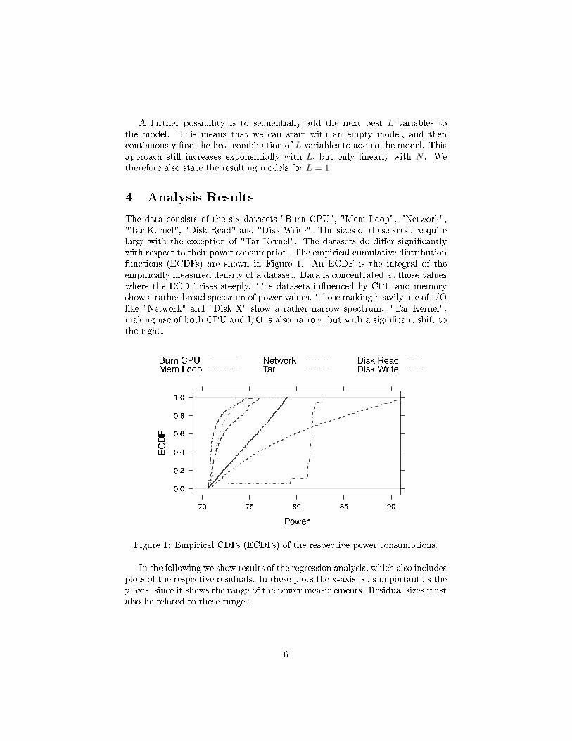
The data consists of the six datasets "Burn CPU", "Mem Loop", "Network","Tar Kernel", "Disk Read" and "Disk Write". The sizes of these sets are quitelarge with the exception of "Tar Kernel". The datasets do di�er signi�cantlywith respect to their power consumption. The empirical cumulative distributionfunctions (ECDFs) are shown in Figure 1. An ECDF is the integral of theempirically measured density of a dataset. Data is concentrated at those valueswhere the ECDF rises steeply. The datasets in�uenced by CPU and memoryshow a rather broad spectrum of power values. Those making heavily use of I/Olike "Network" and "Disk X" show a rather narrow spectrum. "Tar Kernel",making use of both CPU and I/O is also narrow, but with a signi�cant shift tothe right.

Figure 1: Empirical CDFs (ECDFs) of the respective power consumptions.

In the following we show results of the regression analysis, which also includesplots of the respective residuals. In these plots the x-axis is as important as they-axis, since it shows the range of the power measurements. Residual sizes mustalso be related to these ranges.

6

4.1 Burn CPU

The dataset "Burn CPU" consists of 2074 complete data records (withoutN/A values). Both datasets "Burn CPU" and "Mem Loop" are similar inthe sense that power can be explained by using one variable only. Table 1shows the best variables explaining the power, with outliers taken into account,and when removing outliers. It must be noted that it is not clear why e.g.host_df_df.root_free_SQ yields such good results. There are some other hostrelated variables also yielding high correlations. However, for instance the vari-ables perf_instructions and perf_cycles do make sense in a pure CPU stresstest and also well explain the power consumption.

Variable R2 σ % #Outhost_df_df.root_free_SQ 0.992 0.216 0.289 0

0.996 0.146 0.195 12host_df_df.root_used 0.992 0.216 0.289 0

0.996 0.146 0.195 12perf_instructions 0.991 0.232 0.310 0

0.996 0.143 0.191 12perf_cycles 0.991 0.233 0.310 0

0.997 0.144 0.192 12

Table 1: Burn CPU.

Figure 2: Burn CPU residuals for variable host_df_df.root_free_SQ.

Figure 2 shows the model residuals when using a model with only the variablehost_df_df.root_free_SQ as single explanatory variable. There are only a fewoutliers, nevertheless in�uencing σ signi�cantly.

4.2 Memory Loop

The dataset "Mem Loop" consists of 2017 complete data records (without N/Avalues). Table 2 shows the best variables explaining the power,

7

Variable R2 σ % #Outperf_context.switches 0.998 0.268 0.339 0

0.999 0.213 0.270 18perf_cache.references 0.998 0.285 0.361 0

0.999 0.196 0.248 25perf_context.switches_SQ 0.977 0.919 1.163 0

Table 2: Memory Loop.

Figure 3: Loop memory residuals for variable perf_context.switches.

Figure 3 shows the model residuals when using a model with only the variableperf_context.switches as single explanatory variable. Again a few outliers arevisible, which however do not signi�cantly in�uence the results. Also, it isobvious that the residui do exhibit a deterministic component. In fact thisdeterministic dependence could be exploited by further re�ning the regressionmodel, e.g., by adding a sin()-like function. It turns out that this is not reallynecessary since the one-variable model is already good enough such that anymodel extension is super�uous.

4.3 Network

The dataset "Network" consists of 1937 complete data records (without N/Avalues). Table 2 shows the best variables explaining the power,

Figure 4 shows the model residuals when using a model with only the variablehost_interface_if_octets.eth1_tx as single explanatory variable. This variablemakes sense when keeping in mind that the workload mainly stresses the networkcard. Furthermore, Table 3 and Figure 4 show that although two variables areenough to explain the power consumption, there are a few outliers that do havea signi�cant in�uence in the result. Removing only 13 out of 1937 data recordsincreases R2 to 0.98 for one, and 0.99 for two variables.

8

Variable R2 σ % #Outhost_interface_if_octets.eth1_tx 0.954 0.178 0.247 0

0.983 0.106 0.147 13host_interface_if_packets.eth1_rx 0.953 0.181 0.251 0

0.980 0.117 0.163 13host_interface_if_packets.eth1_tx 0.951 0.183 0.255 0

0.981 0.114 0.159 13

perf_cycles + 0.967 0.152 0.211 0host_interface_if_packets.eth1_tx 0.991 0.079 0.110 16perf_instructions + 0.967 0.152 0.211 0host_interface_if_packets.eth1_tx 0.991 0.079 0.110 16perf_cycles + 0.967 0.152 0.211 0host_interface_if_octets.eth1_tx 0.991 0.077 0.108 17

Table 3: Network.

Figure 4: Network residuals for variable host_interface_if_octets.eth1_tx.

4.4 Tar Kernel

This dataset contains only 18 complete data records. Inasmuch it was notpossible to reduce the number of explanatory variables by using a full model�rst, and thus, searching for optimal variable combinations had to include all330 explanatory variables (K=330). This was partially compensated by the factthat regression for a small dataset is much faster. Nevertheless, the resultingrun times were much higher. Table 4 and Figure 5 show the regression results.It can be seen that mainly host oriented variables perform best, e.g., number ofblocked processes, disk writing load, but also the load averages.

4.5 Disk Read

This dataset contains 2018 complete data records. As can be seen in Tables 5and 6, and Figure 6 there are a few outliers that have a signi�cant impacton the model accuracy. Removing them results in a su�cient �t though. We

9

Variable R2 σ %host_processes_ps_state. 0.911 0.661 0.816blocked_value

host_processes_ps_state. 0.911 0.660 0.816blocked_value_SQ

host_disk.sda_disk_time_write_SQ 0.911 0.661 0.817

host_cpu.2_cpu.wait_value_SQ + 0.984 0.290 0.358host_load_load_midterm_SQpid_kB_rd_s_SQ + 0.983 0.295 0.364host_load_load_midterm_SQhost_cpu.2_cpu.wait_value_SQ + 0.983 0.300 0.370host_load_load_shortterm_SQ

Table 4: Tar kernel.

Figure 5: Tar kernel residuals for variables host_cpu.2_cpu.wait_value_SQ +host_load_load_midterm_SQ.

also computed models for the optimal triple of variables, which however didnot improve the model quality signi�cantly. We thus omitted them in Table 5.Interestingly single variables do not include disk related variables, but whensequentially adding variables, pid_kB_rd_s_SQ turns up at place third, so itis de�nitely related to the power consumption.

Table 6 shows that for six variables R2 reaches up to 0.98 without outliers,more variables though do not improve the accuracy any more.

4.6 Disk Write

This dataset contains again 2018 non-empty data records. Similar to "DiskRead", this dataset also su�ers from a handful of severe outliers. Figure 7and Tables 7 and 8 show the details. Here it can be seen that power for thisworkload can be best described without using disk related variables. In generalthe models perform a little worse for disk related workload (read and write),

10

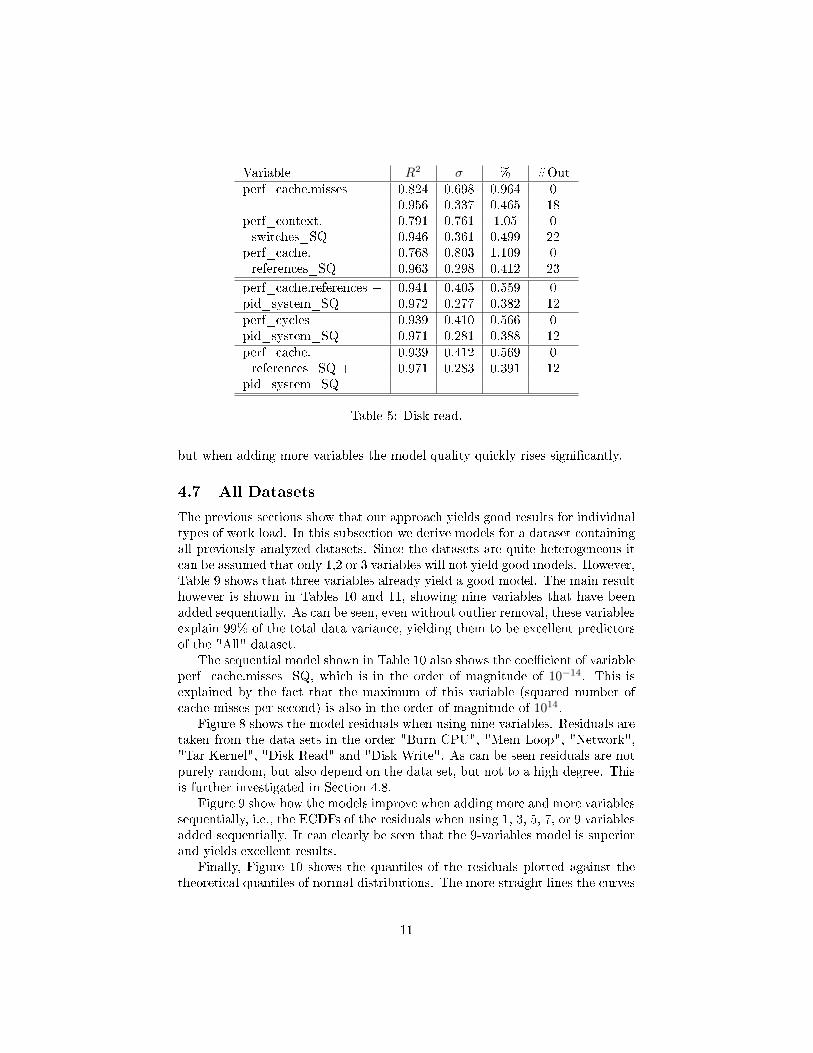
Variable R2 σ % #Outperf_cache.misses 0.824 0.698 0.964 0

0.956 0.337 0.465 18perf_context. 0.791 0.761 1.05 0switches_SQ 0.946 0.361 0.499 22

perf_cache. 0.768 0.803 1.109 0references_SQ 0.963 0.298 0.412 23

perf_cache.references + 0.941 0.405 0.559 0pid_system_SQ 0.972 0.277 0.382 12perf_cycles + 0.939 0.410 0.566 0pid_system_SQ 0.971 0.281 0.388 12perf_cache. 0.939 0.412 0.569 0references_SQ + 0.971 0.283 0.391 12

pid_system_SQ

Table 5: Disk read.

but when adding more variables the model quality quickly rises signi�cantly.

4.7 All Datasets

The previous sections show that our approach yields good results for individualtypes of work load. In this subsection we derive models for a dataset containingall previously analyzed datasets. Since the datasets are quite heterogeneous itcan be assumed that only 1,2 or 3 variables will not yield good models. However,Table 9 shows that three variables already yield a good model. The main resulthowever is shown in Tables 10 and 11, showing nine variables that have beenadded sequentially. As can be seen, even without outlier removal, these variablesexplain 99% of the total data variance, yielding them to be excellent predictorsof the "All" dataset.

The sequential model shown in Table 10 also shows the coe�cient of variableperf_cache.misses_SQ, which is in the order of magnitude of 10−14. This isexplained by the fact that the maximum of this variable (squared number ofcache misses per second) is also in the order of magnitude of 1014.

Figure 8 shows the model residuals when using nine variables. Residuals aretaken from the data sets in the order "Burn CPU", "Mem Loop", "Network","Tar Kernel", "Disk Read" and "Disk Write". As can be seen residuals are notpurely random, but also depend on the data set, but not to a high degree. Thisis further investigated in Section 4.8.

Figure 9 show how the models improve when adding more and more variablessequentially, i.e., the ECDFs of the residuals when using 1, 3, 5, 7, or 9 variablesadded sequentially. It can clearly be seen that the 9-variables model is superiorand yields excellent results.

Finally, Figure 10 shows the quantiles of the residuals plotted against thetheoretical quantiles of normal distributions. The more straight lines the curves

11

Variable R2 σ % #Outperf_cache.misses 0.824 0.698 0.964 0

0.956 0.337 0.465 18perf_cache.misses_SQ 0.909 0.502 0.694 0

0.956 0.337 0.465 17pid_kB_rd_s_SQ 0.919 0.474 0.655 0

0.970 0.280 0.387 18pid_system_SQ 0.937 0.417 0.576 0

0.971 0.274 0.379 19perf_cache.references_SQ 0.949 0.377 0.520 0

0.979 0.236 0.326 14perf_instructions_SQ 0.951 0.367 0.508 0

0.980 0.231 0.320 14

Table 6: Disk read, sequentially adding single variables.

are, the more they follow a normal distribution. As can be seen, the model usingthe optimal triple (O3), as well as the model using 9 variables show a large regionbetween -3.5 and 2.5 where they follow a normal distribution nicely. Outsidethis region, both models show di�erences in their tails caused by outliers.

4.8 Global Model Applied to all Datasets

Table 11 shows how a model with 9 variable explains all data sets in total. Thequestion now is how this global model performs when applied to each individualdata set. Table 12 shows the respective regression results. As can be seen theglobal model performs outstandingly well, and explains the power consumptionfor every single dataset. The only data set having some deviances is "DiskWrite", but when removing only 12 outliers, the situation dramatically changes,and 97% of the variance is explained, which is an excellent result.

5 Power Consumption of a single Process

The above derived models describe the power consumption of a computer bya combination of system wide variables Yi, i = 1, . . . , I, as well as variablesXjl, j = 1, . . . , J describing individual process pl, l = 1, . . . , L. Let the powerconsumption of a computer with no load be denoted by P0 (the intercept), andthe respective coe�cients of the regression model be called αi for system widevariables, and βj for per process variables. The linear model then relates thepower consumption P of a computer in the following way:

P = P0 +

I∑i=1

αiYi +

J∑j=1

βj

L∑l=1

Xjl. (1)

12

Figure 6: Disk read residuals for variables perf_cache.references +pid_system_SQ.

By setting

Sj =

L∑l=1

Xjl,

(1) can be written as

P = P0 +

I∑i=1

αiYi +

J∑j=1

βjSj . (2)

In order to derive the power caused by an individual process Pl, we assumethat the relevant system wide variables are caused by the processes, which arethemselves described by their individual per process variables. To verify thisassumption we explained the system wide variables host_irq_irq.26_value andhost_disk.sda_disk_merged_write by the per process variables. The resultingR2 were 0.956 and 0.99, i.e., they can be almost entirely explained by per processvariables. We therefore write

Yi =

J∑j=1

γijSj , (3)

and adapt (1) to a new form

P = P0 +

I∑i=1

αi

J∑j=1

γijSj +

J∑j=1

βjSj

= P0 +

J∑j=1

Sj

(βj +

I∑i=1

αiγij

)

13

Variable R2 σ % #Outperf_cache.misses 0.768 0.588 0.822 0

0.925 0.297 0.415 19perf_context.switches_SQ 0.635 0.738 1.032 0

0.955 0.211 0.295 22perf_context.switches 0.628 0.745 1.0414 0

0.919 0.281 0.393 23

perf_cycles_SQ + 0.895 0.396 0.553 0host_cpu.0_cpu. 0.967 0.216 0.303 12system_value_SQ

perf_instructions_SQ + 0.895 0.397 0.555 0host_cpu.0_cpu. 0.967 0.217 0.303 12system_value_SQ

perf_context. 0.893 0.400 0.560 0switches_SQ +

host_cpu.0_cpu. 0.970 0.202 0.283 14system_value_SQ

perf_context.switches + 0.901 0.385 0.539 0perf_instructions_SQ + 0.969 0.211 0.295 10host_cpu.0_cpu.system_value_SQ

perf_context.switches + 0.901 0.385 0.539 0perf_cycles_SQ + 0.969 0.211 0.296 10host_cpu.0_cpu.system_value_SQ

perf_cache.misses + 0.900 0.386 0.539 0perf_instructions_SQ + 0.970 0.203 0.283 16host_cpu.0_cpu.system_value_SQ

Table 7: Disk write.

= P0 +J∑

j=1

ηjSj (4)

by de�ning

ηj = βj +

I∑i=1

αiγij .

Thus, we now describe the global power consumption by per process variablesonly. At this point we can derive the power Pl as caused by pl to be

Pl =

J∑j=1

ηjXjl. (5)

14

Variable R2 σ % #Outperf_cache.misses 0.761 0.588 0.822 0

0.925 0.297 0.415 19perf_cache.misses_SQ 0.816 0.524 0.732 0

0.919 0.308 0.430 20host_cpu. 0.865 0.449 0.627 00_cpu.system_value_SQ 0.932 0.296 0.414 21

perf_context.switches_SQ 0.906 0.374 0.523 00.973 0.196 0.274 13

Table 8: Disk write, sequentially adding single variables.

Figure 7: Disk write residuals for variables perf_context.switches +perf_instructions_SQ + host_cpu.0_cpu.system_value_SQ.

Figure 8: All datasets residuals for the sequential model using 9 variables shownin Table 10.

15

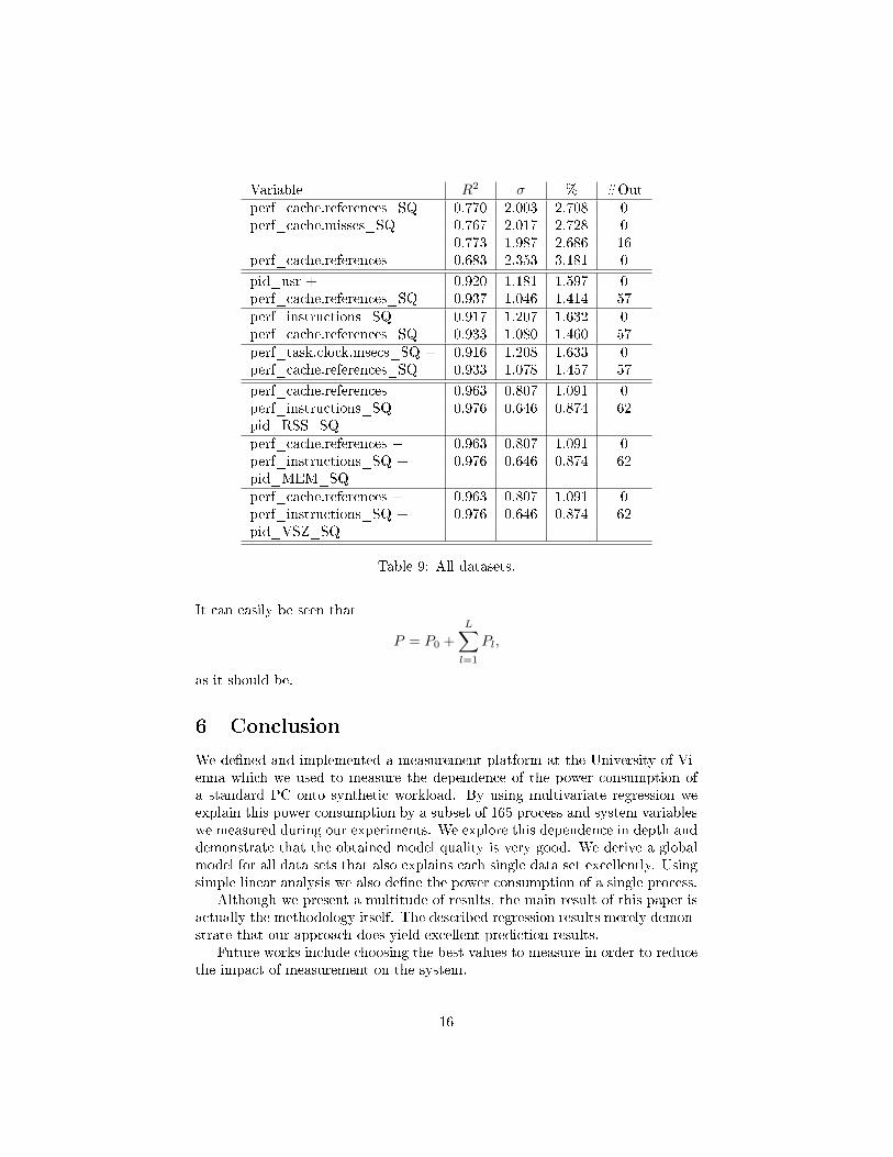
Variable R2 σ % #Outperf_cache.references_SQ 0.770 2.003 2.708 0perf_cache.misses_SQ 0.767 2.017 2.728 0

0.773 1.987 2.686 16perf_cache.references 0.683 2.353 3.181 0

pid_usr + 0.920 1.181 1.597 0perf_cache.references_SQ 0.937 1.046 1.414 57perf_instructions_SQ + 0.917 1.207 1.632 0perf_cache.references_SQ 0.933 1.080 1.460 57perf_task.clock.msecs_SQ + 0.916 1.208 1.633 0perf_cache.references_SQ 0.933 1.078 1.457 57

perf_cache.references + 0.963 0.807 1.091 0perf_instructions_SQ + 0.976 0.646 0.874 62pid_RSS_SQperf_cache.references + 0.963 0.807 1.091 0perf_instructions_SQ + 0.976 0.646 0.874 62pid_MEM_SQperf_cache.references + 0.963 0.807 1.091 0perf_instructions_SQ + 0.976 0.646 0.874 62pid_VSZ_SQ

Table 9: All datasets.

It can easily be seen that

P = P0 +

L∑l=1

Pl,

as it should be.

6 Conclusion

We de�ned and implemented a measurement platform at the University of Vi-enna which we used to measure the dependence of the power consumption ofa standard PC onto synthetic workload. By using multivariate regression weexplain this power consumption by a subset of 165 process and system variableswe measured during our experiments. We explore this dependence in depth anddemonstrate that the obtained model quality is very good. We derive a globalmodel for all data sets that also explains each single data set excellently. Usingsimple linear analysis we also de�ne the power consumption of a single process.

Although we present a multitude of results, the main result of this paper isactually the methodology itself. The described regression results merely demon-strate that our approach does yield excellent prediction results.

Future works include choosing the best values to measure in order to reducethe impact of measurement on the system.

16

Variable Coe� Coe� ErrIntercept 7.056e+01 7.781e-03perf_cache.misses_SQ -8.195e-15 1.671e-15pid_usr 8.401e-02 1.879e-04host_irq_irq.26_value 6.882e-03 6.278e-05pid_system_SQ 3.717e-03 3.237e-05perf_context.switches 6.266e-04 1.107e-05pid_kB_wr_s 1.737e-04 4.696e-06host_disk.sda_disk_merged_write -5.270e-04 1.930e-05perf_cache.references 1.190e-06 1.357e-08pid_VSZ -1.601e-05 2.064e-07

Table 10: All datasets, regression coe�cients and errors of the coe�cients. Allcoe�cients are signi�cantly di�erent from zero (p-values<1.0E-7)

Acknowledgment

This work was done during a short term scienti�c mission (Cost action 0804)of Georges Da Costa (IRIT, Toulouse, France) to the University of Vienna(Austria) from 8, January to 12, February 2010, and was supported by theEuropean Commission.

References

[1] R. Joseph and M. Martonosi, �Run-time power estimation in high perfor-mance microprocessors,� in ISLPED '01: Proceedings of the 2001 interna-tional symposium on Low power electronics and design. ACM, 2001.

[2] I. Kadayif, T. Chinoda, M. Kandemir, N. Vijaykirsnan, M. J. Irwin, andA. Sivasubramaniam, �vec: virtual energy counters,� in PASTE '01: Pro-ceedings of the 2001 ACM SIGPLAN-SIGSOFT workshop on Program anal-ysis for software tools and engineering. ACM, 2001.

[3] X. Ma, M. Dong, L. Zhong, and Z. Deng, �Statistical power consumptionanalysis and modeling for gpu-based computing,� in SOSP Workshop onPower Aware Computing and Systems (HotPower '09), 2009.

[4] S. Rivoire, P. Ranganathan, and C. Kozyrakis, �A comparison of high-levelfull-system power models.� in HotPower, F. Zhao, Ed. USENIX Association,2008.

[5] M. J. Crawley, Statistics: An Introduction using R. Wiley, 2005,iSBN 0-470-02297-3. [Online]. Available: http://www.bio.ic.ac.uk/research/crawley/statistics/

17

Variable R2 σ % #Outperf_cache.misses_SQ 0.767 2.017 2.728 0

0.773 1.987 2.686 16pid_usr 0.916 1.209 1.635 0

0.935 1.062 1.437 56host_irq_irq.26_value 0.950 0.934 1.263 0

0.971 0.706 0.955 63pid_system_SQ 0.966 0.772 1.043 0

0.977 0.634 0.857 48perf_context.switches 0.976 0.651 0.881 0

0.986 0.491 0.663 65pid_kB_wr_s 0.980 0.593 0.801 0

0.989 0.426 0.577 78host_disk. 0.983 0.541 0.732 0sda_disk_merged_write 0.989 0.430 0.581 92

perf_cache.references 0.985 0.508 0.687 00.990 0.407 0.550 77

pid_VSZ 0.991 0.402 0.544 00.995 0.282 0.382 90

Table 11: All datasets, sequentially adding single variables.

Figure 9: All datasets, ECDFs of the residuals, when using 1, 3, 5, 7, or 9variables added sequentially. O3 denotes the optimal combination of 3 variables.

18

Figure 10: All datasets, Q-Q-plot of the residuals, when using 1, 3, 5, 7, or 9variables added sequentially. O3 denotes the optimal combination of 3 variables.

Data set R2 σ % #Out"Burn CPU" 0.992 0.225 0.3 0"Mem Loop" 0.999 0.144 0.24 0"Network" 0.944 0.196 0.27 0

0.974 0.134 0.19 17"Tar Kernel" 0.965 0.556 0.69 0"Disk Read" 0.946 0.389 0.54 0

0.974 0.265 0.36 11"Disk Write" 0.89 0.407 0.57 0

0.965 0.221 0.31 12

Table 12: Applying the global model from Table 11 to the respective data sets.

19