Methodology for Numerical Simulation of Trabecular Bone ... · Simulation of Trabecular Bone...

Copyright © 2011 Tech Science Press CMES, vol.79, no.3, pp.159-182, 2011

Methodology for Numerical Simulation of TrabecularBone Structures Mechanical Behavior

M.A. Argenta1, A.P. Gebert2, E.S. Filho3, B.A. Felizari4 and M.B. Hecke5

Abstract: Various methods in the literature proposesequations to calculate thestiffness as a function of density of bone tissue such as apparent density and ashdensity among others[Helgason, Perilli, Schileo, Taddei, Brynjolfsson and Vice-conti, 2008]. Other ones present a value of an equivalent elasticity modulus, ob-tained by statistical adjustments of curves generated through mechanical compres-sion tests over various specimens[Chevalier, Pahr, Allmer, Charlebois and Zysset,2007; Cuppone, Seedhom, Berry and Ostell, 2004]. Bone tissue is a material with-different behaviors according to the scale of observation. It has a complex com-posite hierarchical structure, which is responsible for assign optimal mechanicalproperties. Its characteristics, composition and mechanical properties depend onthe level at which the material is evaluated[Fritsch and Hellmich, 2007; Hamed,Lee and Jasiuk, 2010]. This paper presents a methodology for computational me-chanical simulation of trabecular bones based on the mechanical properties of theirelements, hydroxyapatite, type I collagen and non-collagenous proteins with water,and the concentration of these ones obtained by microtomography.

Keywords: Microtomography, Trabecular Bone, Properties of Materials, Biome-chanics, Computer Simulation, Finite Elements.

1 Introduction

Bone is a highly specialized form of conjunctive tissue whose function is to sup-port the higher vertebrates. It is a complex living tissue in which the extracellularmatrix is mineralized, providing rigidity and strength to the skeleton, but maintain-ing certain degree of elasticity. Its composition can be separated into an organic

1 PPGMNE, UFPR, Polytechnic Center - CESEC, Curitiba, Parana, Brazil.2 Department of Odontology, PUC, Curitiba, Parana, Brazil.3 Vita Hospital, BR 116, Curitiba, Parana, Brazil.4 Civil Engineering, UFPR, Polytechnic Center - CESEC, Curitiba, Parana, Brazil.5 Civil Construction Department, UFPR, CESEC, Curitiba, Parana, Brazil.

160 Copyright © 2011 Tech Science Press CMES, vol.79, no.3, pp.159-182, 2011

matrix, composed almost entirely of collagen, and an inorganic matrix, composedprimarily of calcium and phosphate in the form of hydroxyapatite[Bilezikian, Raiszand Rodan, 1996]. Hydroxyapatite (Ca5(PO4)6OH) is responsible for the stiffnessof bone tissue and the fibers of type I collagen by its elasticity[Behari, 2009]. Thetrabecular bone, object of study of this article, in its composition in microscale,is characterized by a bone matrix formed by lamellae and lacunae, composed byspecialized cells such as osteoblasts (bone formation), osteoclasts (bone resorp-tion) and osteocytes. At nanoscale, bone tissue is composed primarily of fibroustype I collagen (tropocollagen) that interact with molecules of hydroxyapatite in anaqueous medium in presence of non-collagenous proteins (NCP).

The ability to simulate the internal structure of a bone in microscale may suggest animprovement in surgical techniques, for example, knee arthroscopy, which is nowcommonly done to treat the damaged meniscus cartilage, the construction of fullprosthesis knee, anterior cruciate ligament reconstruction or treatment of cartilagemicrofractures, among others. In some of these cases, it is necessary to implant pinsor screws for fixation. The identification of mechanical properties of bone tissueof each patient can help, for example, in choosing the best type of screw for eachspecific case, improving both the surgical procedure and postoperative morbidity.In addition, the proposed model can assist in the development of equipment andtooling systems for surgery applied to the trabecular bone tissue.

In the literature, within the area of biomechanics and bioengineering, it is pos-sible to find works that proposes ways to characterize the bone tissue, mainlyseeking tounderstand its mechanical properties.Some authors have presented val-ues of the elastic modulus for human bone tissue[Cuppone, Seedhom, Berry andOstell, 2004], [Chevalier, Pahr, Allmer, Charlebois and Zysset, 2007], [Uchiyama,Tanizawa, Muramatsu, Endo, Takahashi and Hara, 1999], equine[Leahy, Smith,Easton, Kawcak, Eickhoff, Shetye and Puttlitz, 2010], swine[Teo, Si-Hoe, Keh andTeoh, 2006], muridae[Cory, Nazarian, Entezari, Vartanians, Muller and Snyder,2010], through destructive tests on reference volumes of bone samples with statis-tically significant amounts, and some of them also considered samples extracted inmany directions for tests[Mittra, Rubin and Qin, 2005], [Ohman, Baleani, Perilli,Dall’Ara, Tassani, Baruffaldi and Viceconti, 2007]. This methodology providesaindication of the samples mechanical properties, applicable with accuracy onlyover these samples, and providing an approximation to estimated the propertiesin other different trabecular bones. Other authors presented equations for calcu-lating the elasticity modulus based onbone volume ratio, tissue volume[Guo andKim, 2002]and bone tissue density in a representative reference volume [Helgason,Perilli, Schileo, Taddei, Brynjolfsson and Viceconti, 2008], [Rho, Hobatho andAshman, 1995], [Zannoni, Mantovani and Viceconti, 1998], including relations for

Simulation of Trabecular Bone Structures Mechanical Behavior 161

elastic modulus obtained for tension and for compression[Kaneko, Pejcic, Tehran-zadeh and Keyak, 2003]. Some of these equations for the trabecular bone tissuewere reviewed by Helgason, 2008 [Helgason, Perilli, Schileo, Taddei, Brynjolfssonand Viceconti, 2008] for apparent density, ash density and bone volume fraction.This review shows both the lack of standardized testing and the variation of results.In a certain way, these equations can describe an elastic modulus for bone tissue.The problem is that these equations are very varied and different, depending on thelocation from where the tissue was extracted and type of bone density. Even us-ing the same kind of density and a very same location to extract a sample in orderto proceed the calculation, the equations differ from each other. The test condi-tion and size of the specimen theoretically should not influence the determinationof a relationship between density and elastic modulus. However, as each sampleis a single chaotic structure it is impossible to obtain a constant ratio[Helgason,Perilli, Schileo, Taddei, Brynjolfsson and Viceconti, 2008]. There are also otherauthors who presented methods that treat the bone as a material with compositestructure and organized in several levels[Rho, Kuhn-Spearing and Zioupos, 1998].This was made as a way to understand the molecular properties of its elementalconstituents in order to describe the mechanical behavior in these various levelsor scales[Hamed, Lee and Jasiuk, 2010]using techniques of homogenization andmultiscale[Hollister, Brennan and Kikuchi, 1994], [Aoubiza, Crolet and Meunier,1996].

In fact, bone is a material that behaves according to the scale ofobservation sinceit has a complex composite hierarchical structure responsible for its optimal me-chanical properties. The characteristics, composition and mechanical properties ofa bonedepends on the level in which the material is evaluated[Ghanbari and Naghd-abadi, 2009; Norman, Shapter, Short, Smith and Fazzalari, 2008; Rho, Kuhn-Spearing and Zioupos, 1998]. Moreover, all these material structures work togetherto produce the global properties of bone (mechanical, chemical, etc.)[Sansalone,Lemaire and Naili, 2007].The hierarchical structure of bone tissue, starting fromthe elemental constituents, can be composed as follows: first, entry level, there arecollagen fibers in an aqueous medium in the presence of non-collagenous proteins.The next level is represented by the fibers of interfibrillar collagen containing hy-droxyapatite crystals, thus, producing mineralized collagen fibers. In the followinglevel, the mineralized collagen fibers are surrounded by a matrix of extrafibrilarhydroxyapatite, consisting of hydroxyapatite in an aqueous medium in the pres-ence of non-collagenous proteins. The final level, addressed in this article, is thelevel where the mineralized collagen fibers in a matrix of extrafibrilar hydroxyap-atite join together, leaving some empty spaces, known as lacunae, to form a singlelamellae[Jasiuk and Ostoja-Starzewski, 2004; Nikolov and Raabe, 2008; Sansa-


lone, Lemaire and Naili, 2007]. A model in visiblescale, in this case microscale,which represents satisfactorily the mechanical properties of a bone, should considerall levels of its hierarchical structure[Sansalone, Lemaire and Naili, 2007]studyingat each scale which properties are governed by the structural organization at lowerlevels[Weiner and Traub, 1992].

This paper presents a methodology for computer simulation for the mechanical be-havior ofspecific trabecular bone samples, starting from the mechanical propertiesof the elementary constituents of bone tissue, hydroxyapatite, type I collagen andother, existing at the nanometric level, and its concentration in bone tissue, givenby the gray level ofmicrotomography transverse slices and an estimation of thevariation in volume fraction of each constituent, based on minimum and maximumvalues from the literature.

2 Description of the method

The bone tissue is a living material and therefore its mechanical properties are func-tions of numerous biological variables as quantity of certain hormones, biomechan-ical variables such as physical exercises that the individual undergoes, and physi-cal variables, as the bone density that are different in each individual [Compston,Mellish, Croucher, Newcombe and Garrahan, 1989]. The analysis of the materialpresented in this article is restricted to a bone tissue of a person with certain charac-teristics of life, at the very instant when the regeneration and reabsorption functionsceased, what is marked by the time of the sample extraction. The tissue propertiesdegradation was minimized in order to make the acquisition of µCT images andmechanical tests reveal the original properties of the extracted bone.

2.1 Trabecular bonesamples

Samples of autologous and homologous human tissue are used for analysis. Its useis approved by the Ethics Committee in Research of the National Health Council,case number 285/2011, which deals with the partnership between the Group of Bio-engineering, Federal University of Parana and VitaHospital. Patients who agreedto participate in research, through the donation of residual bone of the tibia aftersurgery, signed a consent form. The surplus graft or bone piece is recorded, pack-aged and sent with a registration number that identifies the patient. The medic incharge is the only one with access to the patient’s identification. Patient’s identityis not revealed in any step of the study.

Samples were taken from surgical discards of human tibia removed during surgi-cal procedures on the knee with variable sizes and shapes. These samples wereprepared using a trephine drill (Drill Trephine, Neodent, Curitiba - PR - Brazil)


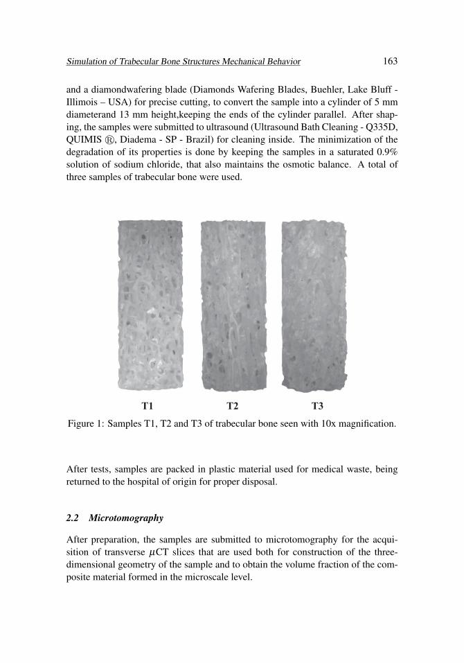
and a diamondwafering blade (Diamonds Wafering Blades, Buehler, Lake Bluff -Illimois – USA) for precise cutting, to convert the sample into a cylinder of 5 mmdiameterand 13 mm height,keeping the ends of the cylinder parallel. After shap-ing, the samples were submitted to ultrasound (Ultrasound Bath Cleaning - Q335D,QUIMIS r, Diadema - SP - Brazil) for cleaning inside. The minimization of thedegradation of its properties is done by keeping the samples in a saturated 0.9%solution of sodium chloride, that also maintains the osmotic balance. A total ofthree samples of trabecular bone were used.

T1 T2 T3

Figure 1: Samples T1, T2 and T3 of trabecular bone seen with 10x magnification.

After tests, samples are packed in plastic material used for medical waste, beingreturned to the hospital of origin for proper disposal.

2.2 Microtomography

After preparation, the samples are submitted to microtomography for the acqui-sition of transverse µCT slices that are used both for construction of the three-dimensional geometry of the sample and to obtain the volume fraction of the com-posite material formed in the microscale level.


2.2.1 Aquisition and Reconstruction of µCT Slices

The device used to acquire microtomography was the SkyScan 1172 high resolution(rSkyscan, Kontich - Belgium). The acquisition of radiological images for eachsample was made using 80 kV (kilovolt) of power and 124 mA (microamperes)current flow with aluminum 0.5 mm (millimeters)filtering and a exposure time of6 s (seconds) to eachrotation step of 0.42007◦ for a total of 360◦, resulting in 857images. The sample was positioned at a distance of 166.51 mm from the X-raysource, ensuring an accuracy of 5.25 micrometers (micron) for each side for eachbasic unit of the digital image, the pixel, after the reconstruction of tomographicslices.

The reconstruction of transverse slices of the samples is done by a modified Feld-kamp algorithm and four computers connected in parallel for data processing, us-ing the reconstruction program NRecon (rSkyscan, Kontich - Belgium), version1.6.3.0. The results are digital images with resolution of 1360 x 1360 pixels, with atotal amount of 2572 images representing cross sections of the bone sample alongthe height. After the reconstruction, algorithms are applied for cleaning images,removing noise and defects that arise from errors during the process of acquisitionand reconstruction, such as ring artifacts or beam hardening.

2.2.2 Segmentation and Generation of a representative three-dimensionalgeometricmodel

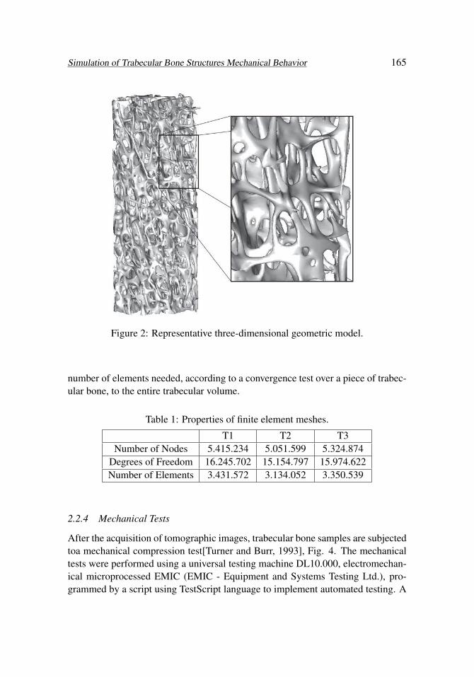
Segmentation of µCT transverse slices is a process in which the pixelscorrespond-ing to the bone tissue are selected from images and identified to be used in thegeneration of a representative three-dimensional geometric model. This procedureis done through the software ScanIP (Simpleware r, Innovation Centre, Exeter,United Kingdom) generating three-dimensional solidsthat describe the geometricstructure of the trabecular bone sample. Figure 2 illustrates the representative three-dimensional geometric model generated throughScanIP for a sample of trabecularbone.

From the representative three-dimensional geometric model described in the STLformat is possible to generate a tetrahedral finite element mesh for stress analysis.

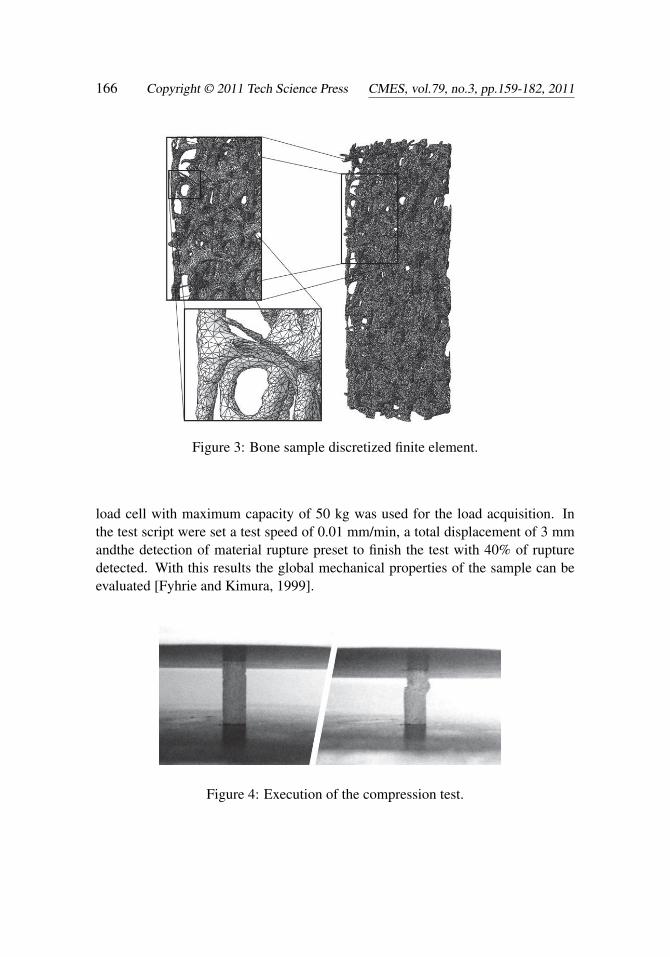
2.2.3 Finite Elements Discretization

The discretization in finite element mesh of three-dimensional geometry was doneusing the software Amirar(Visage Imaging, Inc. San Diego, CA, USA). Fig. 3shows a view of the samples after the generation of finite element mesh.

The finite element meshes of bone samples were generated to have an average of3.3 million elements.This value was found through the extrapolation of the total


Figure 2: Representative three-dimensional geometric model.

number of elements needed, according to a convergence test over a piece of trabec-ular bone, to the entire trabecular volume.

Table 1: Properties of finite element meshes.

T1 T2 T3Number of Nodes 5.415.234 5.051.599 5.324.874

Degrees of Freedom 16.245.702 15.154.797 15.974.622Number of Elements 3.431.572 3.134.052 3.350.539

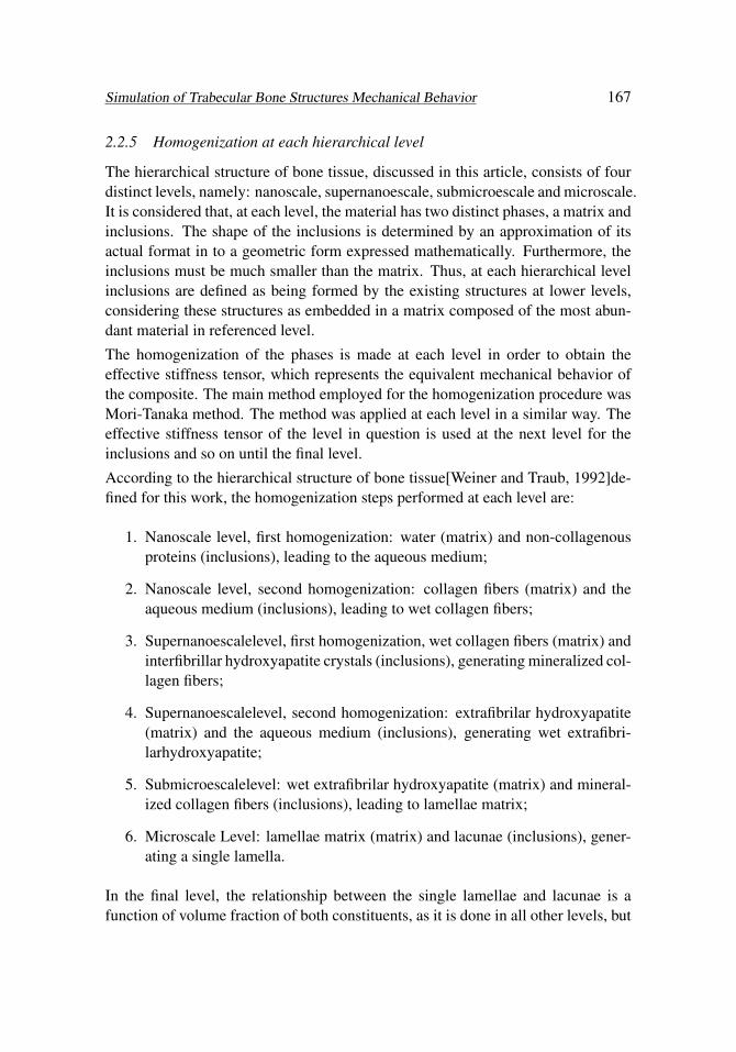
2.2.4 Mechanical Tests

After the acquisition of tomographic images, trabecular bone samples are subjectedtoa mechanical compression test[Turner and Burr, 1993], Fig. 4. The mechanicaltests were performed using a universal testing machine DL10.000, electromechan-ical microprocessed EMIC (EMIC - Equipment and Systems Testing Ltd.), pro-grammed by a script using TestScript language to implement automated testing. A


Figure 3: Bone sample discretized finite element.

load cell with maximum capacity of 50 kg was used for the load acquisition. Inthe test script were set a test speed of 0.01 mm/min, a total displacement of 3 mmandthe detection of material rupture preset to finish the test with 40% of rupturedetected. With this results the global mechanical properties of the sample can beevaluated [Fyhrie and Kimura, 1999].

Figure 4: Execution of the compression test.


2.2.5 Homogenization at each hierarchical level

The hierarchical structure of bone tissue, discussed in this article, consists of fourdistinct levels, namely: nanoscale, supernanoescale, submicroescale and microscale.It is considered that, at each level, the material has two distinct phases, a matrix andinclusions. The shape of the inclusions is determined by an approximation of itsactual format in to a geometric form expressed mathematically. Furthermore, theinclusions must be much smaller than the matrix. Thus, at each hierarchical levelinclusions are defined as being formed by the existing structures at lower levels,considering these structures as embedded in a matrix composed of the most abun-dant material in referenced level.

The homogenization of the phases is made at each level in order to obtain theeffective stiffness tensor, which represents the equivalent mechanical behavior ofthe composite. The main method employed for the homogenization procedure wasMori-Tanaka method. The method was applied at each level in a similar way. Theeffective stiffness tensor of the level in question is used at the next level for theinclusions and so on until the final level.

According to the hierarchical structure of bone tissue[Weiner and Traub, 1992]de-fined for this work, the homogenization steps performed at each level are:

1. Nanoscale level, first homogenization: water (matrix) and non-collagenousproteins (inclusions), leading to the aqueous medium;

2. Nanoscale level, second homogenization: collagen fibers (matrix) and theaqueous medium (inclusions), leading to wet collagen fibers;

3. Supernanoescalelevel, first homogenization, wet collagen fibers (matrix) andinterfibrillar hydroxyapatite crystals (inclusions), generating mineralized col-lagen fibers;

4. Supernanoescalelevel, second homogenization: extrafibrilar hydroxyapatite(matrix) and the aqueous medium (inclusions), generating wet extrafibri-larhydroxyapatite;

5. Submicroescalelevel: wet extrafibrilar hydroxyapatite (matrix) and mineral-ized collagen fibers (inclusions), leading to lamellae matrix;

6. Microscale Level: lamellae matrix (matrix) and lacunae (inclusions), gener-ating a single lamella.

In the final level, the relationship between the single lamellae and lacunae is afunction of volume fraction of both constituents, as it is done in all other levels, but


with these fractions calculated according to the gray value from the µCT transverseslices. Through this, the effective stiffness tensor, in microscale, specific to thetrabecular bone sample under analysis is obtained.

The Mori-Tanaka method was chosen for the homogenization of the properties ofthe composites formed at each hierarchical level of bone tissue, precisely becauseof their use for this purpose[Fritsch and Hellmich, 2007], [Hamed, Lee and Jasiuk,2010]. Moreover, the values that the method provides are coherent for the homog-enization of composites mechanical properties[Klusemann and Svendsen, 2010].

The Mori-Tanaka method [Mori and Tanaka, 1973] uses the Eshelby equivalentinclusion method [Eshelby, 1957] and the fact that the average deformation in aellipsoidal matrix circumscribed to an ellipsoidal inclusion is also zero. In addi-tion, the method approximates the interaction between the phases of the compositeassuming that each inclusion i is incorporated, at a time, in an infinite matrix whichis subject to a uniform load applied away from the inclusion, resulting in a fieldof average stresses and strains in the matrix σM and εM, respectively[Mura, 1993].Therefore, the deformation in a simple inclusion iis calculated by,

εi = AiεM (1)

where, Ai is the influence tensor for a single inclusion[Klusemann and Svendsen,2010]. The influence tensor can be given by,

Ai =[I+EC−1

M (Ci−CM)]−1

(2)

being, I the fourth order identity tensor, E Eshelby tensor for aninclusion, depend-ing on the elastic properties of the matrix and the shape of inclusions, Ci the inclu-sion stiffness tensor and CM the matrix stiffness tensor[Klusemann and Svendsen,2010].

Eq. (2) is defined, according Mura, 1993, in the case of ellipsoidal inclusions fora single inclusion[Mura, 1993]. The shapes of inclusions as spherical, cylindrical,ellipsoidal cylinder, can be derived from the ellipsoidal formulation by adjusting theEshelby tensor, according to the lengths of the axes of the ellipsoid[Mura, 1993].For example, for a sphere, the axes of the ellipsoid have equallengthswhile to acylinder one axis has an infinite length and so on.

The volume fraction of inclusions and matrix are related as follows[Hamed, Leeand Jasiuk, 2010],

fi+ fM=1 (3)

The effective stiffness tensor for the composite, according to the Mori-Tanaka


method, can be written as[Benveniste, 1987],

Ce f =CM+ fi (Ci−CM)Ai( fiAi+ fMI)−1 (4)

This method can be interpreted in the sense that each inclusion behaves like anisolated inclusion in the matrix being εM a far deformationsfield[Benveniste, 1987].

The Eshelby tensor used in Eq. (2) is a fourth-order tensor that relates the eigen-strains, depending on the shape and material of the inclusions, and the matrix, withthe total deformation of the composite[Mura, 1993]. If both materials, in the inclu-sion and in the matrix are isotropic or transversely isotropic materials, the Eshelbytensor has an analytical solution, given respectively by Mura[Mura, 1993] e Li eDunn[Li and Dunn, 1998].

In the case of the inclusions being in a matrix of anisotropic material, it is neces-sary to calculate the Eshelby tensor through a numerical method[Klusemann andSvendsen, 2010]. The Eshelby tensor can be calculated by a surface integral, pa-rameterized on the surface of a unit sphere[Mura, 1993], given by,

Ei jkl=1

8πCMi jkl

∫ 1

−1

∫ 2π

0

[Gim jn

(ξ

)+G jmin

(ξ

)]dθdξ 3 (5)

where, Gim jn

(ξ

)is the tensor of Green’s functions, derived from the method of

Green’s functions for the description of eigenstrains[Mura, 1993].

Using the numerical method of Gauss-Legendre integration, the Eq. (5) is rewrittenas,

Ei jkl=1

8πCMi jkl

∫ np

p=1

∫ nq

q=1

[Gim jn

(θq,ξ 3 p

)+G jmin

(θq,ξ 3 p

)]WqWp (6)

where, np isthenumberof Gauss points in directionξ 3, nq thenumberof Gauss pointsin the angular directionθ , Wp and Wq therespective Gauss weights [Desrumaux,Meraghni and Benzeggagh, 2001].Calculating the Eshelbytensor is possible to cal-culate the influence tensor of the inclusions and thus find the effective stiffnesstensor for the composite.

2.2.6 Volumetric Fractions

The volumetric fractions in the microscale, are calculated according to the graylevel of pixels in the transverse microtomographycslices. All other volumetric frac-tions, in the other levels are derived from elementary constituents fractions thatexists in the single lamellae level (micro) through percentages described in the lit-erature for each elementary constituents[Fritsch and Hellmich, 2007], [Hamed, Leeand Jasiuk, 2010].


The lacunae, its size and quantity in a certain part of the trabecular bone are closelyrelated to bone remodeling, being directly proportional to the osteoclastic activ-ity[Fritsch and Hellmich, 2007], responsible for bone resorption. The size of thelacunae varies with diameters about 0.1 µm and lengths from 1 to 3 µm[Jasiukand Ostoja-Starzewski, 2004]with an approximately ellipsoidal shape. Fractions ofthese lacunae occur within each voxel[Tkachenko, Slyfield, Tomlinson, Daggett,Wilson and Hernandez, 2009]. These fractions can be identified by the gray valueof µCT transverse slices. Based on the survey of segmentation, where the lowerand upper limits of the gray values within bone pieces are found and knowing thatthe fraction of lacunae inside a cubic voxel size about 5.0 µm edges may varyabout 16% with a variance of 1.9%[Tkachenko, Slyfield, Tomlinson, Daggett, Wil-son and Hernandez, 2009] it is possible to create an approximated linear correla-tion between the gray value of the transverse µCT images with volume fraction oflamellae matrix for each voxel.

Figure 5: Correlation of the voxel gray value and its corresponding volume fractionof lamellae matrix.

AccordingtoHamedand Lee [Hamed, Lee and Jasiuk, 2010], the volumetric frac-tions for each elementary constituent of bone tissue present in the lamellae ma-trix, can be defined keeping the mineral fraction around 50%[Fritsch and Hellmich,2007].

Table 2: Volume fractions of the elementary constituents for the lamellae matrix[Hamed, Lee and Jasiuk, 2010].

Constituent Volumetric Fraction [%]Colagen 35

Hydroxyapatite 50NCP 5Water 10


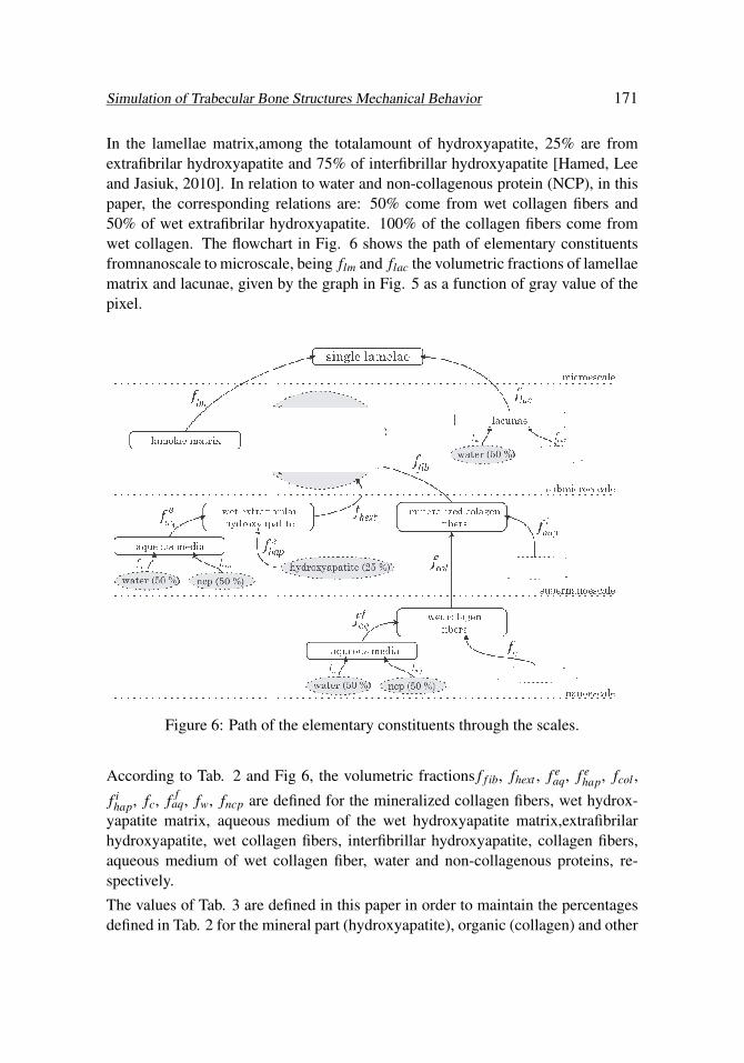
In the lamellae matrix,among the totalamount of hydroxyapatite, 25% are fromextrafibrilar hydroxyapatite and 75% of interfibrillar hydroxyapatite [Hamed, Leeand Jasiuk, 2010]. In relation to water and non-collagenous protein (NCP), in thispaper, the corresponding relations are: 50% come from wet collagen fibers and50% of wet extrafibrilar hydroxyapatite. 100% of the collagen fibers come fromwet collagen. The flowchart in Fig. 6 shows the path of elementary constituentsfromnanoscale to microscale, being flm and flac the volumetric fractions of lamellaematrix and lacunae, given by the graph in Fig. 5 as a function of gray value of thepixel.

Figure 6: Path of the elementary constituents through the scales.

According to Tab. 2 and Fig 6, the volumetric fractions f f ib, fhext , f eaq, f e

hap, fcol ,

f ihap, fc, f f

aq, fw, fncp are defined for the mineralized collagen fibers, wet hydrox-yapatite matrix, aqueous medium of the wet hydroxyapatite matrix,extrafibrilarhydroxyapatite, wet collagen fibers, interfibrillar hydroxyapatite, collagen fibers,aqueous medium of wet collagen fiber, water and non-collagenous proteins, re-spectively.

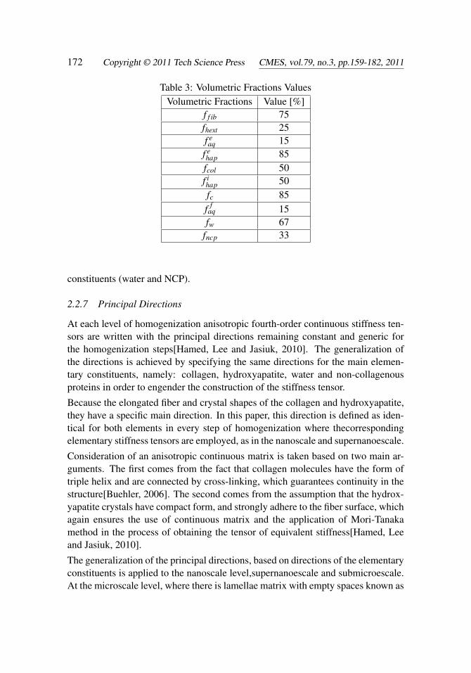
The values of Tab. 3 are defined in this paper in order to maintain the percentagesdefined in Tab. 2 for the mineral part (hydroxyapatite), organic (collagen) and other


Table 3: Volumetric Fractions ValuesVolumetric Fractions Value [%]

f f ib 75fhext 25f eaq 15

f ehap 85fcol 50f ihap 50fc 85f faq 15fw 67

fncp 33

constituents (water and NCP).

2.2.7 Principal Directions

At each level of homogenization anisotropic fourth-order continuous stiffness ten-sors are written with the principal directions remaining constant and generic forthe homogenization steps[Hamed, Lee and Jasiuk, 2010]. The generalization ofthe directions is achieved by specifying the same directions for the main elemen-tary constituents, namely: collagen, hydroxyapatite, water and non-collagenousproteins in order to engender the construction of the stiffness tensor.

Because the elongated fiber and crystal shapes of the collagen and hydroxyapatite,they have a specific main direction. In this paper, this direction is defined as iden-tical for both elements in every step of homogenization where thecorrespondingelementary stiffness tensors are employed, as in the nanoscale and supernanoescale.

Consideration of an anisotropic continuous matrix is taken based on two main ar-guments. The first comes from the fact that collagen molecules have the form oftriple helix and are connected by cross-linking, which guarantees continuity in thestructure[Buehler, 2006]. The second comes from the assumption that the hydrox-yapatite crystals have compact form, and strongly adhere to the fiber surface, whichagain ensures the use of continuous matrix and the application of Mori-Tanakamethod in the process of obtaining the tensor of equivalent stiffness[Hamed, Leeand Jasiuk, 2010].

The generalization of the principal directions, based on directions of the elementaryconstituents is applied to the nanoscale level,supernanoescale and submicroescale.At the microscale level, where there is lamellae matrix with empty spaces known as


lacunae, a different assumption is made for the local axes of each single lamellaerepresented by a voxel.The equivalent stiffness tensors obtained in this level foreach voxel or lamellae, were made considering their principal direction as the samedirections of the trabeculae.

A procedure for coordinate transformation of the fourth order tensor, given by Eq.(8), is used to obtain the equivalent stiffness tensor of voxel, written in global di-rections [Lai, Rubin and Krempl, 2010].

C′i jkl = QmiQn jQrkQslCmnrs (7)

being, Cmnrs the equivalent stiffness tensor of voxel obtained by the process ofhomogenization of Mori-Tanaka for the last hierarchical level, microscale, Qi j thematrix of directive cosines (the transformation matrix between local and globalaxes) e C′i jkl the equivalent stiffness tensor of the voxel in the total directions.

2.2.8 Anisotropic stiffness tensor of each finite element

The anisotropic stiffness tensor of each finite element is calculated using the ap-proximation of Voigt[Mura, 1993]. Voigt’s method is known from the literature forpresenting overestimated values, being used as the upper limit[Hamed, Lee and Ja-siuk, 2010]for the analysis of homogenization methods. However, because inside afinite element it is an idealized material (a bunch of piled cubes or voxels), whichdoes not define matrix and inclusions, the method can be applied as a first approachto the problem. The stiffness tensor of each finite element (Celem) is calculated fromthe stiffness tensor calculated for each voxel representing the bone (Ci

vox), based onthe volumetric fractions of each voxel ( f i

vox) present within the finite element by itsrespective stiffness tensor.

Celem=∫ nve

i=1f ivoxC

ivox (8)

being, nve the total number of voxels within the finite element in question.

After proceeding a survey about which voxels are present within each finite ele-ment, the Voigt’s approximated homogenization method is applied in order to ob-tain the stiffness tensors for each one of these elements.

The volumetric fractions of each voxel are nothing else than very volume of them.Each voxel has cubic shape with 5,25 µm edges (function of the microtomographyparameters) with a total volume of 144,70 µm3. The sum of the volumetric frac-tions of all voxels within certain finite element should be approximately equal tothe volume of the same finite element.


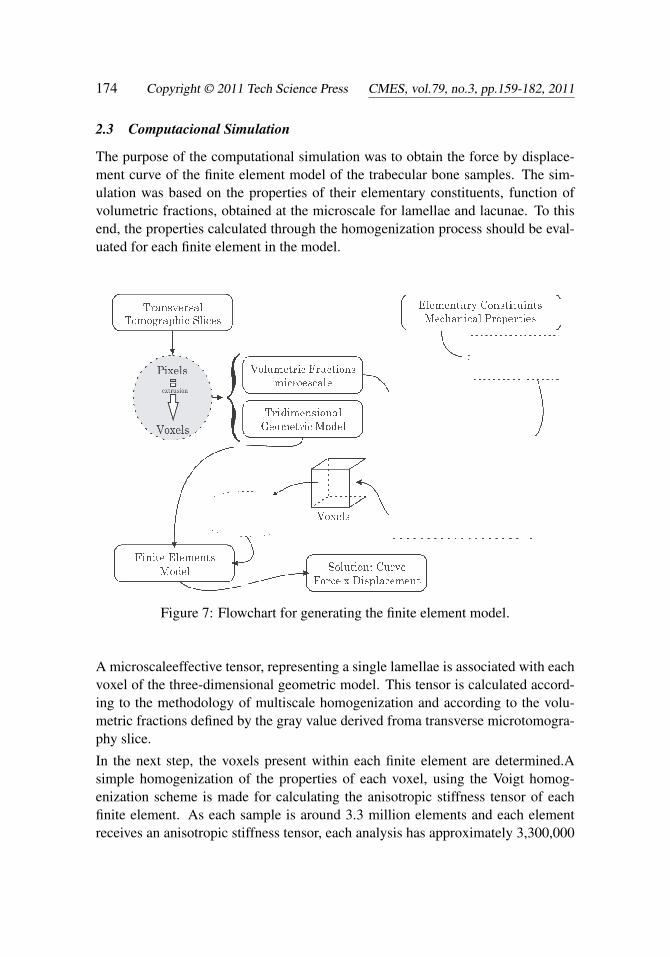
2.3 Computacional Simulation

The purpose of the computational simulation was to obtain the force by displace-ment curve of the finite element model of the trabecular bone samples. The sim-ulation was based on the properties of their elementary constituents, function ofvolumetric fractions, obtained at the microscale for lamellae and lacunae. To thisend, the properties calculated through the homogenization process should be eval-uated for each finite element in the model.

Figure 7: Flowchart for generating the finite element model.

A microscaleeffective tensor, representing a single lamellae is associated with eachvoxel of the three-dimensional geometric model. This tensor is calculated accord-ing to the methodology of multiscale homogenization and according to the volu-metric fractions defined by the gray value derived froma transverse microtomogra-phy slice.

In the next step, the voxels present within each finite element are determined.Asimple homogenization of the properties of each voxel, using the Voigt homog-enization scheme is made for calculating the anisotropic stiffness tensor of eachfinite element. As each sample is around 3.3 million elements and each elementreceives an anisotropic stiffness tensor, each analysis has approximately 3,300,000


stiffness tensors.

The finite element model is solved through the application of concentrated loadsrepresenting a total load of 150 N in the upper nodes of the model, constrainingthe displacements of the nodes of the upper surface to have equal displacement.Boundary conditions are inserted in the lower nodes, considering them fixed, forthe simulation of mechanical testing and obtaining the force by displacement com-putational curve.

An application in python, divided into modules, was developed for these proce-dures. The final result of this algorithm is a computer simulation, through the finiteelement method, of the linear elastic part of the physical mechanical test. The res-olution of the computer simulation took about three days for each bone sample andwas only possible through the Linux operating system Ubuntu 4.10 LTS (LucidLynx) (http://www.ubuntu-br.org/).

The algorithm was written in python, because of the ease implementation and pro-ductivity offered by this programming language. After concluding the simulationand obtaining a graphic of force by displacement, the evaluation and comparisonof the results contrasting with physical mechanical tests were done.

The calculation of elastic moduli for both physical tests and the results of the com-puter simulations were made according to the slopes obtained with trend lines forthe linear part of the force by displacement curves. These values were calculated asfunctions of the total height and the cross-sectional area of the samples, accordingto the Eq. (9).

E = IFDhA

(9)

where, IFD trend line slope for the force by displacement graphs, h total height ofthe samples (13 mm), A the cross-sectional area and E the elastic modulus of thesample.

3 Results

Graphics comparing the physical mechanical tests and the computer simulation ofthe mechanical tests, using finite elements for samples T1, T2 and T3 are shown inFig. 8. Due to the size and complexity of computer simulation, comparisons arerestricted to linear elastic regime.

4 Discussion and Conclusions

Bone tissue is a complex material in its geometry, mechanical properties, physicaland biological characteristics. The complexity of the issue justifies the numerous


F=633,93D-164,1

F=663,03D-F=1460,9D 415,19

F=1520,3D

F=785,92D-347,34

F=837,1D

0

20

40

60

80

100

120

140

160

180

200

220

240

260

0 0,1 0,2 0,3 0,4 0,5 0,6 0,7 0,8Deslocamento [mm]

Amostra T1

Amostra T2

Amostra T3

Forç

a [N

]

Figure 8: Force vs. Displacement comparison graphic for the sample T1, T2 andT3, respectively.

studies where the main subject is the bone, both cortical and trabecular one. Thecharacteristics studied such as mechanical properties are disparate and almost neverdefine or standardize a generic behavior.

Indeed the mechanical characterization of a bone is almost an impossible missionwhen adopted an simplified approach since the properties of it are functions ofmany biological variables as the amount of certain hormones, biomechanical vari-ables such as amount of exercise that a person undergoes and physical variablessuch as bone density, which one is different in every person atdifferent momentsin life. This occurs because bone is a living tissue that undergoes constant damageand recovery (bone remodeling)to the extent of changing the entire human skeletonin approximately eight years[Behari, 2009].

The approach of bone tissue as a composite material consisting of a multiscalehierarchical structure in which, at each level, all the structures compounding thematerial work together to produce the global properties of the bones (mechanical,chemical, etc.), is currently the most accepted approachproducing the most consis-tent results. This assertion can be made based on the latest publications on the me-chanical behavior of bone tissue[Coelho, Fernandes and Rodrigues, 2011; Hackl,Ilic and Gilbert, 2010; Hambli, 2010; 2011; Hambli, Katerchi and Benhamou,


2011; Hamed, Lee and Jasiuk, 2010; Ilic, Hackl and Gilbert, 2010; Levengood, Po-lak, Wheeler, Maki, Clark, Jamison and Johnson, 2010; Podshivalov, Fischer andBar-Yoseph, 2011].

However, the mere consideration of bone tissue as a hierarchical and multiscalematerial does not guarantee the general characterization since it undergoes a highvariation in its mechanical properties. The method proposed in this paper for a bet-ter approximation of the real and correct mechanical properties in a specific bonesample is to measure the amounts of bone constituents at a certain level or scale,more specifically, in the microscale, and use these measures in the stiffness tensorsformulation. Theses tensors represent the mechanical properties for each represen-tative volume where it is possible to identify certain variation of these properties,being these representative volumes the voxels.

There are many difficulties on implementing a model with these proposed features,starting from the complexity of the multiscale mathematical procedure andhomog-enization, and ending with enormity of the computer model to represent a smallsample of 5 mm in diameter and 13 mm in height. The justification for this modelliesin the possibility of implementing large computational models due to the lat-est generation of computers available in ordinary consumers market in the years of2010 and 2011. Also, another justificationis the possibility of using very high levelprogramming languages, as python, what guarantees a high productivity.

A model with this level of complexity can provide much more than a simple com-parison with mechanical compression tests. Its evolution in terms of implementingfeatures as damage, fracture, and other non-linear mechanical theories, can lead toa deeper understanding about bone tissue’s behavior and consequently improve theprocess of computer simulation for these structures. The material damage is visi-ble by observing the displacement-force curve of physical compression tests. Forexample, the curve for sample T2, Fig. 8, shows the starting point of damage afterthe linear elastic regime followed by a major loss of rigidity. In the curves, anotherdepicted point deserves some commentaries. This is the point of stiffness initialgain, which can be understood as a failure (and even rupture) of the trabeculae incontact with the surface of the load stage due to the small contact area, which isabout 10 to 15% of the total cross-sectional samples. This rupture occurs until thepoint that the packaging of these fractured trabeculae generates a sufficient con-tact area for the whole sample to be requested and the structure as a whole startto work mechanically. Even so, it is possible to note that the elastic regime is notas linear as it is supposed to be according to the theoretical definition. There is alittle damage occurring with this scheme. This damage can be a residue of failureand continuous breaking offin the structures that initially collapsed, or a failure ofsmall trabecular structures, arranged in improper positions in relation to the stress


concentration, what causes a fast elevationin the tension level rapidly achieving thecollapse.

Regarding the results obtained through the methodology proposed in this paper,there are discrepancies in the computational results in relation to the physical re-sults, from approximately 4% for samples 1 and 2 and 6% in sample 3. This errormaybe a result from several variables involved in development of the employedmethodology. It can be related to the application of Voigt’s homogenization theory,classically known in the literature for overestimate stiffness values for compos-ites[Hamed, Lee and Jasiuk, 2010], or the occurrence of damage and failure ofstructures, previously to the linear regime, causing a global behavior distinct fromthe behavior calculated in the computer modeling. In addition, the methodologyitself may need some adjustments. Another factor to be considered is to soak theends of the bone sample in a resin or similar material to ensure an area of load trans-fer that does not begin with an early damage on parts of the end structure during thesample’s physical compression tests, what makes possible even a tensile test. Thisapproach requires that the contact surface between the resin and the bone must becalculated as well as the mechanical properties of the resin should be known.

The presented methodology for trabecular bone tissue computational simulationwas found to be approximately consistent with the results of physical tests. Itmeans that, in a certain way, the methodology can be applied in the predictionof stresses and strains intrabecular bone structures. The main consideration on theproposed methodology is the fact that it can characterize specific trabecular bonestructures departing from same values of stiffness tensors for the elementary con-stituents. This fact is illustrated by the variation in the force displacement graphicsof each sample in computer simulations. Being function of microtomography pa-rameters, this characterization is a noninvasive technique that according to somespecial parameters can even be applied in vivo.

Cases in which the methodology is applicable are those ones where there was nodamage in the trabecular structure and also when only an idea about the structurebehavior in linear elastic regime is needed.

Despite of its limitations, the methodology was found to be efficient on the charac-terization of specific bone structures, achieving global mechanical properties sim-ilar to the same properties evaluated through mechanical testes according to everydifferent samples of human trabecular bones.

Thus, studies in specific locations of certain individual’s trabecular bone tissue,with certain characteristics, according to the time when his functions of regenera-tion and resorption ceased can employ the proposed methodology in order to obtainthe structure’s response about the stress and strain relation on an elastic regime.


Acknowledgement: CAPES - Coordination for the Improvement of Higher Ed-ucation People, Bioengineering Group of the Federal University of Parana, LAMIR- Laboratory of minerals and rocks LABNANO - Laboratory of NanomechanicsProperties of Surfaces and Thin Films, Vita Hospital, CONEP - National Boardof Health and National Committee for Ethics in Research, LAGEMA - Laboratoryof Geotechnical and Environmental Materials, Laboratory of Analysis of Mortar,Laboratory of High Performance Concrete and JulianoScremin Translations.

References

Aoubiza, B.; J. M. Crolet; A. Meunier (1996): On the mechanical character-ization of compact bone structure using the homogenization theory. J Biomech,29(12), 1539-1547.

Behari, J. (Ed.) (2009): Biophysical bone behavior, 501 pp., John Wiley & Sons(Asia), Singapore.

Benveniste, Y. (1987): A new approach to the application of Mori-Tanaka’s theoryin composite materials. Mechanics of Materials, 6(2), 147-157.

Bilezikian, J. P.; L. G. Raisz; G. A. Rodan (1996): Principles of bone biology,xx,1398p.,[1316]p. of plates pp., Academic Press, San Diego ; London.

Buehler, M. J. (2006): Nature designs tough collagen: Explaining the nanostruc-ture of collagen fibrils. Proceedings of the National Academy of Sciences, 103(33),12285-12290.

Chevalier, Y.; D. Pahr; H. Allmer; M. Charlebois; P. Zysset (2007): Validationof a voxel-based FE method for prediction of the uniaxial apparent modulus ofhuman trabecular bone using macroscopic mechanical tests and nanoindentation. JBiomech, 40(15), 3333-3340.

Coelho, P. G.; P. R. Fernandes; H. C. Rodrigues (2011): Multiscale modeling ofbone tissue with surface and permeability control. J Biomech, 44(2), 321-329.

Compston, J. E.; R. W. E. Mellish; P. Croucher; R. Newcombe; N. J. Garrahan(1989): Structural mechanisms of trabecular bone loss in man. Bone and Mineral,6(3), 339-350.

Cory, E.; A. Nazarian; V. Entezari; V. Vartanians; R. Muller; B. D. Snyder(2010): Compressive axial mechanical properties of rat bone as functions of bonevolume fraction, apparent density and micro-ct based mineral density. J Biomech,43(5), 953-960.

Cuppone, M.; B. B. Seedhom; E. Berry; A. E. Ostell (2004): The longitudinalYoung’s modulus of cortical bone in the midshaft of human femur and its correla-tion with CT scanning data. Calcif Tissue Int, 74(3), 302-309.


Desrumaux, F.; F. Meraghni; M. L. Benzeggagh (2001): Generalised Mori-Tanaka scheme to model anisotropic damage using numerical Eshelby tensor. JCompos Mater, 35(7), 603-624.

Eshelby, J. D. (1957): The Determination of the Elastic Field of an EllipsoidalInclusion, and Related Problems. Proc R Soc Lon Ser-A, 241(1226), 376-396.

Fritsch, A.; C. Hellmich (2007): ’Universal’ microstructural patterns in corticaland trabecular, extracellular and extravascular bone materials: Micromechanics-based prediction of anisotropic elasticity. J Theor Biol, 244(4), 597-620.

Fyhrie, D. P.; J. H. Kimura (1999): Cancellous bone biomechanics. J Biomech,32(11), 1139-1148.

Ghanbari, J.; R. Naghdabadi (2009): Nonlinear hierarchical multiscale modelingof cortical bone considering its nanoscale microstructure. J Biomech, 42(10), 1560-1565.

Guo, X. E.; C. H. Kim (2002): Mechanical consequence of trabecular bone lossand its treatment: a three-dimensional model simulation. Bone, 30(2), 404-411.

Hackl, K.; S. Ilic; R. Gilbert (2010): Multiscale modeling for cancellous bone byusing shell elements. Shell Structures: Theory and Applications, Vol 2, 249-252.

Hambli, R. (2010): Application of Neural Networks and Finite Element Compu-tation for Multiscale Simulation of Bone Remodeling. J Biomech Eng-T Asme,132(11), -.

Hambli, R. (2011): Multiscale prediction of crack density and crack length accu-mulation in trabecular bone based on neural networks and finite element simulation.Int J Numer Meth Bio, 27(4), 461-475.

Hambli, R.; H. Katerchi; C. L. Benhamou (2011): Multiscale methodology forbone remodelling simulation using coupled finite element and neural network com-putation. Biomech Model Mechan, 10(1), 133-145.

Hamed, E.; Y. Lee; I. Jasiuk (2010): Multiscale modeling of elastic properties ofcortical bone. Acta Mech, 213(1-2), 131-154.

Helgason, B.; E. Perilli; E. Schileo; F. Taddei; S. Brynjolfsson; M. Viceconti(2008): Mathematical relationships between bone density and mechanical proper-ties: A literature review. Clin Biomech, 23(2), 135-146.

Hollister, S. J.; J. M. Brennan; N. Kikuchi (1994): A homogenization samplingprocedure for calculating trabecular bone effective stiffness and tissue level stress.J Biomech, 27(4), 433-444.

Ilic, S.; K. Hackl; R. Gilbert (2010): Application of the multiscale FEM to themodeling of cancellous bone. Biomech Model Mechan, 9(1), 87-102.


Jasiuk, I.; M. Ostoja-Starzewski (2004): Modeling of bone at a single lamellalevel. Biomech Model Mechan, 3(2), 67-74.

Kaneko, T. S.; M. R. Pejcic; J. Tehranzadeh; J. H. Keyak (2003): Relationshipsbetween material properties and CT scan data of cortical bone with and withoutmetastatic lesions. Med Eng Phys, 25(6), 445-454.

Klusemann, B.; B. Svendsen (2010): Homogenization methods for multi-phaseelastic composites: Comparisons and Benchmarks. Technische Mechanik, (4), 374-386.

Lai, W. M.; D. Rubin; E. Krempl (2010): Introduction to continuum mechanics.4th ed., xiv, 520 p. pp., Butterworth-Heinemann/Elsevier, Amsterdam; Boston.

Leahy, P. D.; B. S. Smith; K. L. Easton; C. E. Kawcak; J. C. Eickhoff; S.S. Shetye; C. M. Puttlitz (2010): Correlation of mechanical properties within theequine third metacarpal with trabecular bending and multi-density micro-computedtomography data. Bone, 46(4), 1108-1113.

Levengood, S. K. L.; S. J. Polak; M. B. Wheeler; A. J. Maki; S. G. Clark; R. D.Jamison; A. J. W. Johnson (2010): Multiscale osteointegration as a new paradigmfor the design of calcium phosphate scaffolds for bone regeneration. Biomaterials,31(13), 3552-3563.

Li, J. N. Y.; M. L. Dunn (1998): Anisotropic coupled-field inclusion and inhomo-geneity problems. Philos Mag A, 77(5), 1341-1350.

Mittra, E.; C. Rubin; Y. X. Qin (2005): Interrelationship of trabecular mechanicaland microstructural properties in sheep trabecular bone. J Biomech, 38(6), 1229-1237.

Mori, T.; K. Tanaka (1973): Average Stress in Matrix and Average Elastic Energyof Materials with Misfitting Inclusions. Acta Metall Mater, 21(5), 571-574.

Mura, T. (1993): Micromechanics of defects in solids. 2nd, rev. ed. ed., XIII-587pp., Kluwer Academic publ., Dordrecht Boston London.

Nikolov, S.; D. Raabe (2008): Hierarchical modeling of the elastic properties ofbone at submicron scales: The role of extrafibrillar mineralization. Biophys J,94(11), 4220-4232.

Norman, J.; J. G. Shapter; K. Short; L. J. Smith; N. L. Fazzalari (2008): Mi-cromechanical properties of human trabecular bone: a hierarchical investigationusing nanoindentation. J Biomed Mater Res A, 87(1), 196-202.

Ohman, C.; M. Baleani; E. Perilli; E. Dall’Ara; S. Tassani; F. Baruffaldi; M.Viceconti (2007): Mechanical testing of cancellous bone from the femoral head:Experimental errors due to off-axis measurements. J Biomech, 40(11), 2426-2433.

Podshivalov, L.; A. Fischer; P. Z. Bar-Yoseph (2011): 3D hierarchical geometric


modeling and multiscale FE analysis as a base for individualized medical diagnosisof bone structure. Bone, 48(4), 693-703.

Rho, J. Y.; M. C. Hobatho; R. B. Ashman (1995): Relations of Mechanical-Properties to Density and Ct Numbers in Human Bone. Med Eng Phys, 17(5),347-355.

Rho, J. Y.; L. Kuhn-Spearing; P. Zioupos (1998): Mechanical properties and thehierarchical structure of bone. Med Eng Phys, 20(2), 92-102.

Sansalone, V.; T. Lemaire; S. Naili (2007): Multiscale modelling of mechanicalproperties of bone: study at the fibrillar scale. Cr Mecanique, 335(8), 436-442.

Teo, J. C. M.; K. M. Si-Hoe; J. E. L. Keh; S. H. Teoh (2006): Relationship be-tween CT intensity, micro-architecture and mechanical properties of porcine verte-bral cancellous bone. Clin Biomech, 21(3), 235-244.

Tkachenko, E. V.; C. R. Slyfield; R. E. Tomlinson; J. R. Daggett; D. L. Wilson;C. J. Hernandez (2009): Voxel size and measures of individual resorption cavitiesin three-dimensional images of cancellous bone. Bone, 45(3), 487-492.

Turner, C. H.; D. B. Burr (1993): Basic biomechanical measurements of bone: Atutorial. Bone, 14(4), 595-608.

Uchiyama, T.; T. Tanizawa; H. Muramatsu; N. Endo; H. E. Takahashi; T.Hara (1999): Three-dimensional microstructural analysis of human trabecular bonein relation to its mechanical properties. Bone, 25(4), 487-491.

Weiner, S.; W. Traub (1992): Bone structure: from angstroms to microns. FASEBJ, 6(3), 879-885.

Zannoni, C.; R. Mantovani; M. Viceconti (1998): Material properties assignmentto finite element models of bone structures: a new method. Med Eng Phys, 20(10),735-740.

Methodology for Numerical Simulation of Trabecular Bone ... · Simulation of Trabecular Bone...

Documents

Transcript of Methodology for Numerical Simulation of Trabecular Bone ... · Simulation of Trabecular Bone...