Methodology for Development of Live Load Models for Refined Analysis of Short and Medium-Span Highway Bridges

Giorgio Anitoria, Joan R. Casasa,* and Michel Ghosnb

a Department of Civil and Environmental Engineering, Technical University of Catalonia, UPC-BarcelonaTech

Jordi Girona 1-3. Campus Nord. Modul C1. 08034 Barcelona, Spain

giorgio.anitori@upc.edu, joan.ramon.casas@upc.edu bThe City College of New York/CUNY, New York, USA

mghosn@ccny.cuny.edu *corresponding author

ABSTRACT: The accuracy of bridge system safety evaluations and reliability assessments obtained through

refined structural and Finite Element (FE) analyses depends not only on the accuracy of the structural model

itself but also on the proper modeling of the maximum traffic loads. While current code-specified live load

models were calibrated to properly reflect the safety levels of bridge structures analyzed using the simplified

methods adopted in bridge design and evaluation manuals, these load models may not lead to accurate results

when implemented during refined structural analysis procedures. Accurate live load models need to be defined

based on a statistical analysis of real traffic data. This paper describes a method to calibrate appropriate live

load models that can be used for advanced analyses of highway bridges. The calibration procedure is demon-

strated using actual truck data collected at a representative weigh-in-motion (WIM) station in New York State.

Extreme value theory is used to project traffic load effects and calculate the maximum effect expected to take

place over different bridge service periods. The proposed calibration methodology is applicable for developing

live load models for different bridge types and different design/assessment codes or standards. Live load mod-

els obtained using the proposed calibration procedure are readily implementable for deterministic refined anal-

yses of highway bridges to produce similar results to those of complex traffic load simulations. Examples are

presented that describe how results of such calibrated live load models would be used in engineering practice.

Keywords: live load, refined analysis, weigh in motion, highway bridges, code calibration, bridge assessment

1 INTRODUCTION

One of the most challenging aspects of performing refined analyses for the safety assessment of highway

bridge systems is the determination of the live load model that accurately captures the effects of traffic loads

on a bridge under study. During reliability-based calibrations of bridge codes and specifications, truck traffic

data are typically analyzed to provide generic live load models that can be used during the design of new bridges

or the safety evaluation of existing ones (Nowak, 1999; Moses, 2001). These models require positioning a set

of concentrated loads (sometimes in combination with distributed loads) having specific intensities at critical

locations on bridge decks. Alternatively, live load models may be presented as load effects on specific bridge

components. The live load models adopted in North American specifications, such as those of the American

Association of Highway and Transportation Officials (AASHTO, 2014) or the Canadian Standards (CAN-CSI,

2014), have been calibrated for use with simplified single beam analysis procedures that utilize tabulated load

distribution factors to account for the lateral distribution of the load to parallel beams in multi-girder bridges.

For multi-girder two-lane bridges, the existing live load models, in combination with the associated load distri-

bution factors, were derived assuming that heavy truck events are due to the crossing over the bridge of two

side-by-side trucks of equal weights (Nowak, 1999; Zokaie, Mish, & Imbsen 1995). Adjustments are then made

for one-lane and multi-lane bridges using multiple-presence factors. Because the calibration assumes that the

load effects on two-lane bridges are due to two side-by-side trucks of equal weight, the current live load models

may not be applicable when a more refined analysis, such as a FE analysis or a grillage analysis, is necessary

to study the response of a specific bridge component or structural detail. Also, because truck traffic volumes

and weights vary considerably between regions and between locations, region-specific or even site-specific live

load models that reflect actual traffic conditions may be needed (Sivakumar, Ghosn, & Moses, 2011). Input

data for the development of live load models are best collected using WIM data because these systems collect

unbiased information on truck weights, geometric characteristics and headways to provide a good representa-

tion of the actual traffic conditions and the probability of multiple truck presence on a bridge deck.

While complex probabilistic simulations can be directly used to study the effects of traffic loads on highway

bridges, such simulations require excessive computational effort and are beyond the normal procedures used in

engineering practice. Instead, design manuals and specifications should provide simple models that can be

implemented during deterministic structural analysis to facilitate bridge safety assessment processes. As done

in previous code calibration efforts, such live load models should be calibrated by code writing groups to pro-

duce results similar to those obtained when performing complex simulations.

Some researchers have proposed live load models with variable intensities to account for variations due to

bridge span-length and traffic characteristics (Leahy, Obrien, Enright, Hajializadeh, 2015) while others pro-

posed modifications to existing load distribution factors for bridge evaluation purposes (Pelphrey et al., 2008).

However, to the best knowledge of the authors, no previous research considered the development of live load

models that can be used jointly with more accurate structural models to better reflect actual bridge loading

conditions.

This paper proposes a procedure for calibrating live load models appropriate for performing refined analyses

to evaluate the ultimate strength limit state of highway bridges given a representative set of truck WIM data.

The approach can be used for the formulation of live load models that would be applied during a refined deter-

ministic analysis or the reliability analysis of bridge structural systems using 2-D and 3-D refined structural

models. The method is described in this paper using a set of short to medium length simple-span multi-beam

steel composite bridges as example test cases. A set of WIM data collected at one measurement station in New

York State is used to analyze the bending in longitudinal members of the selected bridge population. The pro-

cedure can be easily extended to cover other structural types including simple span or continuous I-beam, box

girder steel and prestressed concrete bridges or truss bridges to calibrate live load models that reflect all effects

of traffic loads on all components. Preliminary results were presented in Anitori, Casas and Ghosn (2016). The

method presented is general and can be applied to develop models applicable for any bridge design standard or

code, such as the AASHTO specifications or the Eurocodes, as long as the WIM data used during the calibration

are representative of the truck traffic at the bridge sites of concern. The generalization of the procedure de-

scribed in this paper to cover different load effects and to consider truck traffic data with different characteristics

is presented in the paper by Anitori, Casas and Ghosn (2017).

2 OBJECTIVES AND PAPER OUTLINE

This study describes how live load models can be calibrated for implementation when performing refined

deterministic analyses of short to medium span bridges. The live load models would be applicable for two

structural safety check cases:

- Design of new bridges: which considers the maximum load over a bridge design life. In this study, the

calibration procedure is illustrated for a 75-year design life specified by AASHTO (2014) with the

understanding that the method is applicable for any design life such as the 100-year service life appli-

cable to the Eurocodes (CEN, 2002).

- Evaluation of existing bridges: which considers a reduced service period. A reduced time period has

been recommended by Moses (2001) during the calibration of the AASHTO Manual of Bridge Evalu-

ation MBE (2011) when existing bridges are inspected on a regular basis. The reduced service rating

period assumes that if a bridge is subjected to some deterioration, the damage is likely to be detected

within the normal inspection period (e.g. the mandatory biennial inspection period in the U.S.) and its

effect on the structure evaluated within the normal rating period (e.g. the 5-year rating cycle used in

the U.S. as per the AASHTO MBE (2011).

The calibration procedure is illustrated in this paper using truck data collected at WIM station ID9121 in

Central New York State. The records from this station consist of 1,149,657 heavy vehicles and an average daily

truck traffic ( ADTT ) of 3861 trucks/day (Ghosn et al., 2015). A comparison of the data collected at this site

to the legal axle and gross weight limits applicable to Upstate New York indicate that the percentage of over-

weight trucks is 15.2 % of the total truck population. This percentage includes trucks issued permits to carry

overweight as well as illegally overweight trucks (Fiorillo & Ghosn, 2014). The WIM data from this site is used

to propose a live load pattern that reflects the maximum load effect on bridges along routes with truck traffic

similar to that observed at that site by extending a procedure previously developed by Ghosn and Sivakumar

(2010), Ghosn, Sivakumar and Miao (2011) and Sivakumar et al. (2011).

Section 3 of this paper describes how the proposed load models are developed to evaluate the maximum

expected load effect in a specific service period based on a representative set of actual truck traffic data ac-

counting for the effect of multiple-presence of trucks. In Section 4, the load effects obtained in the form of

maximum moments are transformed into an equivalent set of concentrated load configurations. This load pat-

tern that produces load effects consistent with those obtained in Section 3 can be directly used for a refined

analysis of bridges where failure of a bridge is defined in terms of reaching its bending strength limit state.

Section 5 presents examples illustrating how the resulting live load models can be applied for checking the

safety of new bridge designs or the rating of existing bridges as refined extensions of current AASHTO proce-

dures.

3 METHODOLOGY

3.1 Effects of Truck Loads on Short to Medium Span Bridges

The maximum load effect on short to medium span bridges in the range of 15 to 60 m is normally governed

by the presence of a single truck per lane (Nowak, 1999). Therefore, the analysis of the load effect on a single

lane is performed by sending the trucks extracted from the WIM database through the appropriate influence

surfaces. The statistical analysis of the truck load effects is performed by simulating the presence of trucks of

random weights and configurations as they cross over a bridge.

In order to study how the bridge geometric characteristics affects the bridge response, a total of 100 bridge

configurations representative of the typical population of steel-composite bridges having the geometric param-

eters shown in Table 1 are considered in this study. The bridges are designed according to AASHTO (1996) to

reflect the basic design of the majority of existing steel girder bridges (Ghosn et al., 2015). The use of the

previous generation design method should not lead to significant differences in the results obtained if the bridges

were designed to follow current specifications because the goal of this work is to develop a load model that

reflects the load distribution of actual truck traffic to the bridge components. In fact, the different specifications

would mostly lead to different member design strengths and would have little influence on load distribution.

Furthermore, the method presented here may be most suitable for the assessment of existing bridges, where a

refined and more accurate analysis is of major interest rather than for the design of new bridges for which the

current methods are known to provide safe structures.

Table 1. Characteristics of composite steel bridge population Steel girder-concrete slab bridges Span length (m) 15, 20, 30, 40, 60 Number of beams 4, 6, 8, 10Beam spacing (m) 1.2, 1.8, 2.4, 3.0, 3.6

Influence surfaces for each bridge in the population are obtained by performing a grillage analysis based on

the methodology presented in Hambly (1991). Plane 2-D grillage models are known to provide a simple yet

accurate approach for calculating the response of bridge superstructures in a computationally efficient proce-

dure. The grillage model consists of a set of frame elements with different mechanical properties: longitudinal

elements accounting for the composite action of the steel beams and the deck’s concrete slab which provide the

bending moment capacity of the bridge superstructure, transverse elements that account for the transverse stiff-

ness of the slab and help distribute the load among the main longitudinal members in combination with special

transverse elements that account for the contribution of bracings and cross beams. A typical representation of a

grillage model is presented in Figure 1.

Figure 1. Grillage model for a six-beam bridge

The first step in the simulation process consists of developing influence surfaces for the response of a point

load of unit intensity when the load is applied at any point on the bridge deck surface. Subsequently, each of

the trucks in the WIM database is sent through each influence surface to obtain each truck’s load response de-

pending on which lane they are assumed to travel in. The trucks are positioned in the most critical transverse

position according to the obtained influence surface ( the one producing the maximum effect) but always within

the lane borders. The results of the simulated load effects (in this case the bending moments) are assembled in

frequency histograms. For example, the maximum moment effects in four beams of a 30 m bridge with 10

beams at 1.8 m calculated for all the trucks in the WIM station 9121 database are assembled into the histograms

presented in Figures 2 and 3 when the trucks are traveling in the edge lane of the bridge or the second lane from

the edge. The plots and other results indicate that the load in wide bridges consisting of six or more beams is

primarily carried by the external two girders when the trucks are travelling in the edge lane of the bridge as-

sumed to be the main traffic lane in this case. The load effect spreads laterally wider when the trucks are trav-

elling in the passing lane. Specifically, Figure 3 and other analysis results show that girders 3 and 4 carry the

highest portion of the load for bridges with six or more beams spaced at 1.8 m center on center.

Figure 2. Histograms of maximum moment in the first four longitudinal members from the edge due to traffic load in lane 1 of a 30 m bridge with 10 beams at 1.8 m.

Figure 3. Histograms of maximum moment in the first four longitudinal members from the edge due to traffic

load in lane 2 of a 30 m bridge with 10 beams at 1.8 m.

3.2 Statistical Analysis of Truck Load Effect Data

Bridges should be evaluated for their ability to support the largest load that may be applied within their

service lives. Because no matter how extensive the WIM database is, there will always be a possibility that it

does not capture the maximum load. Therefore, the data in the load effect histograms obtained from the rec-

orded traffic must be extrapolated to estimate the extreme loads that may cross the bridge within a specific time

reference. Sivakumar et al. (2011), Ghosn, Sivakumar and Miao (2013) and Soriano ,Casas and Ghosn (2016)

observed when studying large numbers of truck WIM databases that the upper tail of the normalized load effect

distribution approaches that of a normal distribution. Specifically, the analysis of data revealed that the upper

5% of the trucks’ load effects can very well fit the upper tail of a normal distribution as illustrated in the case

presented in Figure 4 that shows a plot of the cumulative distribution of the total moment effect of a 40 m bridge

on a normal probability scale. The abscissa shows the moment effect obtained for trucks from the WIM database

normalized by dividing by the effect of the AASHTO HL-93 design loads. The ordinate gives the normal deviate

corresponding to the probability of exceeding a given load effect value as assembled from histograms similar

to those in Figures 2 and 3. When the data fits a straight line, the distribution is considered to follow a normal

distribution. For example, even though the data in Figure 4 does not follow a straight line, the upper 5% of the

data does. When a linear regression of the upper 5% of the data is performed, the coefficient of regression for

this particular case is R2=0.99 where a coefficient close to 1.0 is indicative of an excellent fit. Similar values

for the goodness of fit for data collected from several U.S. regions and states were observed in a large number

of cases analyzed by Sivakumar et al. (2011). This confirms that the tail end of the load effect approaches the

tail end of a normal probability distribution even if the entire dataset does not. Being able to fit the tail into a

normal probability distribution will facilitate the extrapolation of the results as will be discussed further below.

Figure 4. Linear fit of the upper 5% of normalized moments for the total moment on a 40 m span bridge on normal probability scale

Plots similar to the one shown in Figure 4 are drawn for each beam of the bridges analyzed in this study to

obtain the statistics of the equivalent normal distributions whose tail ends match those obtained from the anal-

ysis of the trucks in the WIM database. For example, Table 2 lists the mean values and the standard deviations

of the equivalent normal probability distributions of the moment load effects in the most loaded beams of

bridges of different span-lengths. These statistics are for equivalent normal distributions whose tail ends match

the upper 5% of the load effects of the truck population collected at New York WIM site 9121. The WIM

database consisted of more than one million trucks collected over a 1-year period. It is interesting to observe

that the statistics fall within a very narrow range with a mean of the load effect divided by that of the HL-93

design load being close to zero and the standard deviation is on the average equal to 0.36 for all the cases

considered.

Table 2. Statistics of the normal distributions whose tail end that matches the upper 5% of the load effects of bridges with different span lengths

Span length

(m)

Mean of normal distribution that fits the upper tail of MWIM/MHL93 histogram

Standard Deviation of normal distribution that fits the upper tail of MWIM/MHL93 histogram

15 -0.01 0.39 20 -0.03 0.34 30 -0.02 0.36 40 -0.01 0.37 60 0.00 0.34

As mentioned earlier, the traffic data collected over any limited period of time may be missing the most

extreme trucks that rarely travel on the highway system. Yet, it is these rare extremely heavy trucks that control

the maximum load effect that any bridge should be able to safely support. Therefore, a statistical projection

procedure has to be used to estimate the maximum load effect expected during the bridge’s service life be it the

5-year or 75-year service lives stipulated in the AASHTO MBE (2011) and the design specifications or the 100-

year life in the Eurocodes.

The statistical projection approach proposed by Sivakumar et al. (2011), and implemented by Ghosn et al.

(2013) and Soriano, Casas and Ghosn (2016) is adopted in this study because of its simplicity and accuracy. By

focusing on the tail of the traffic data, this approach avoids the error that may be caused by assuming that the

entire truck histogram follows one of the standard distributions when in reality, as shown in Figures 2 and 3,

the histogram usually follows more complex multi-modal distributions. It is noted that the approach assumes

that the WIM data gathered during the monitoring period is representative of the truck population over the entire

service life of the bridge and that the bridge loading process remains stationary over time. Therefore, it is very

important that the data collection period be carefully planned to collect a substantial amount of data that provide

an adequate statistical representation of the extreme trucks through ensuring a high confidence levels in the

statistics of the upper 5% of the data. (Sivakumar et al., 2011; Soriano et al., 2016).

3.3 Multiple presence of trucks

In general, it has been observed that the maximum load effect in a single lane simply supported bridge is

controlled by individual trucks when the bridge is less than approximately 60 m (200 ft) in length (see for

example Nowak, 1999, Ghosn et al. 2013, Fu , Liu and Bowman 2013, Ghasemi Nowak and Hossein 2016).

However, for multi-lane bridges and longer and continuous spans, the analysis must take into account the prob-

ability that the maximum effect may be due to the presence of more than one truck in different lanes, different

spans or within the same lane when the span length is long. For instance, OBrien and Enright (2011) observed

when analyzing traffic data collected in two European countries (The Netherlands and the Czech Republic) that

for some cases such as bridges with span-lengths on the order of 45 m with high lane distribution factors and

low volumes of traffic, the critical loading scenario may be due to the presence of more than a single truck per

lane. Due to the different truck characteristics observed in the WIM dataset analyzed in this study which shows

that the heaviest trucks are significantly longer than those observed in the Netherlands or the Czech Republic

and also due to the different lane distribution factors observed for the types of multi-girder bridges studied as

compared to the values assumed by OBrien and Enright (2011), it is herein assumed that the case of one truck

per lane or two side-by-side trucks govern as recommended by Nowak (1999), Fu et al. (2013) and Ghassemi

et al. (2016). For example, Figure 5 shows the frequency distribution of the normalized total moment at the

mid-span of a 60 m long single span when one truck is on the bridge and compares it to that obtained when two

trucks are side-by-side. Of course, the two-lane frequency distribution is not simply the double of that of one

lane because the probability of having two side-by-side trucks of the same weight is very small.

Figure 5. Normalized moment histogram for a 60 m (200 ft) span bridge

A study of the effect of multiple truck presence on bridge decks was considered by Nowak (1999) when

analyzing the effects of two-lane loads on bridges. More recently, OBrien and Enright (2011) have also analyzed

the bridge loading taking into account the modeling of same-direction two-lane traffic. Table 3 summarizes the

results of the maximum load effect obtained when following the approach used by Nowak (1999). A correlation

coefficient less than 1.00 indicates that the moment effect due to multi-presence of two trucks cannot simply

be represented by two equal trucks with the same Gross Vehicle Weights (GVW) although it is not excluded a

priori. A correlation coefficient equal to 1.00 indicates that the moment effect due to multi-presence of two

trucks is always caused by two similar trucks with the same GVW. The trucks are partially correlated. Full

correlation is represented by =1.00, partial correlation by =0.50 and no correlation by =0.00. In Table 3 the

parameter Z is the normal standard deviate of the probability of occurrence for a given number of simultaneous

occurrences, N, such that NZ 11 . The return periods, T, given in the last column of Table 3 for different

values of Z are found by extrapolating the load effect database using the normal distribution. These return

periods can then be used to determine which truck weight should be used in each lane to simulate the maximum

load effect.

Table 3. Return periods, T, for different correlation coefficients in two-lane load events.

Number of lanes loaded N Z T

(number of events) (st. norm. prob.) One 20 000 000 5.33 75 years Two =0.00  Lane 1 1 500 000 4.83 5 years

    Lane 2 1 0.00 average

  =0.50 Lane 1 150 000 4.36 6 months

  Lane 2 1 000 3.09 1 day

  =1.00 Lane 1 50 000 4.11 2 months

  Lane 2 50 000 4.11 2 months Following the results in Table 3, Nowak (1999) assumed that trucks in side-by-side configurations represent

1/15 of the truck loading events and the truck weights in side-by-side events are correlated and that the maxi-

mum 75-year load effect can be simulated by placing the maximum 2-month truck in each lane. However, these

assumptions that are based on the limited data available at the time may not be always valid. In fact, analyzing

large numbers of WIM sites in New York, Sivakumar et al. (2011) observed that: 1) the load effects of heavy

trucks do not generally follow normal probability distributions as observed in Figures 2 through 5 but only the

upper 5% in the tail end matches that of fictitious normal distribution; 2) the percentage of trucks involved in

multi-presence events vary with the truck traffic volume represented by the Average Daily Truck Traffic

(ADTT); and 3) The weights of trucks in side-by-side or closely following configurations are uncorrelated. It is

recognized that OBrien and Enright (2011) using a limited set of European traffic data observed that in some

cases the weights of closely spaced trucks show low levels of correlation. Thus, they demonstrated that, in some

cases the loading of two-lane bridges up to 45 m in length is governed by either one truck in only one lane or

two side-by-side trucks, but that in other cases the governing scenario is a mixture of both event types, and that

for longer spans in the range of 35 to 45 m, simulations showed that one truck in one lane in combination with

two trucks in the other lane produce bending moments close to the characteristic 1000-year load. Thus, OBrien

and Enright conclude that “the characteristic 1000-year load shows that for bridges with low lateral transfer,

the critical loading event for bending moment is typically an extremely heavy vehicle in the slow lane (80% to

90% of the 1000-year GVW), sometimes with a standard vehicle (in the range 30 to 50 t) in the fast lane –

which is consistent with Turkstra’s load combination rule. For bending moments in bridges with high lateral

distributions, the characteristic load can be represented by a very heavy vehicle (60% to 80% of 1000-year

GVW) in the slow lane with a moderately heavy vehicle (50 to 60 t) in the fast lane – a variation on Turkstra’s

rule. For shear at the supports, where the lateral distribution tends to be low, the dominant event type is usually

a single extremely heavy truck in the slow lane (75% to 95% of the 1000-year GVW) “.

However, the observations made by OBrien and Enright may not be consistent with the data collected in

other countries or other sites. WIM data analyzed by Sivakumar et al. (2011) have shown that the percentage

of trucks that arrive at a site side-by-side ranges between 1% to 2% for short to medium span bridges up to 60

m in length, with a high value of 6% for long span bridges with heavy truck volumes. In this work, it is assumed

that 2% of the trucks cross a bridge side-by-side with another truck which is consistent with a typical ADTT of

2000.

Figure 6. Correlation of consecutive trucks in lane 1, 2 and 3 and in different lanes (adopted from Ghosn et al., 2015).

Also, as shown in Figure 6, available WIM data from sites in New York State show that there is no correlation

between the weights of trucks close to each other in the same lane or in adjacent lanes (Ghosn et al. 2015).

Hence, given the probability distribution of the load effect of each truck in a side-by-side configuration, the

probability density function of the effect of two trucks can be calculated as:

11112 dxxfxSfSf xxs (1)

where 1x is the effect of the trucks in lane 1 and 2x is the effect of the trucks in lane 2, Sf s is the probability

distribution function of the multi-lane effects for the joint event 21 xxS , ...1xf is the probability distribu-

tion function of the effects of the trucks in lane 1 and ...2xf is the probability distribution function of the

effects of trucks in lane 2. In the study conducted by Ghosn et al. (2013) and Sivakumar et al. (2011), it was

observed that the frequency distributions of the truck weights in different lanes are essentially similar. There-

fore, the same distribution function can be assumed for and ...2xf which is the assumption adopted in

this study following the observation made in previous research (Fiorillo, 2015; Ghosn et al., 2015).

Other than the input parameters, the main difference between the multi-presence approach adopted by Si-

vakumar et al. (2011) and Ghosn et al. (2013) and subsequently by Soriano et al. (2016) compared to that of

Nowak (1999) is that the latter calculates the truck load effect independently for each lane, then assumes dif-

ferent correlations between the weights of the trucks in side-by-side configurations. The approach adopted here

...1xf

finds the load effect of two-lane loads using Equation (1) and then executes the projection using the expected

number of multiple-presence events within the service life, N.

If the tail of the load effect distribution is modeled as the combined effect of two independent normal dis-

tributions, as it can be certainly done when dealing with the upper 5 % maximum effects as explained earlier,

then the convolution approach of Equation (1) simplifies and the resulting probability distribution can be de-

scribed by the tail of a new normal distribution with the statistical parameters calculated as:

21 xxS (2)

222

1 xxS (3)

where 1x and 2x are the mean values of the normal distribution that matches the upper 5% of the actual

distribution of the load effect of the trucks in lane 1 and 2 respectively and 1x and 2x are the related standard

deviations; S and S are the mean and standard deviation of the distribution that matches the tail end of the

combined load effect. It is noted that Eq. (3) can be adjusted to account for the correlation between the weights

of the trucks in lanes 1 and 2 is warranted by the specific of WIM data used.

3.4 Projection of maximum load effect for different service lives

While the effects of individual trucks or a combination of trucks may be represented by histograms such as

those in Figures 2, 3 and 5 or presented in mathematical expressions (such as Equation (1), bridge engineers

are interested in ensuring the safety of bridges when they are exposed to the maximum possible loads that may

take place within the their service lives. The projection of the load effect to find the maximum load in a specific

time interval requires the application of extreme value theory which can be greatly simplified if the upper 5%

of the load effect histograms can be represented by a normal distribution (Ghosn et al., 2011; Sivakumar, et al.,

2011; Soriano et al., 2014,2016). In fact, the maximum load effect of data that fit a normal distribution is known

to follow an Extreme Value Type I (Gumbel) distribution the statistical parameters of which are obtained by

means of the following equations (Ang & Tang, 2007):

event

N

N

ln2 (4)

N

NNu eventeventN

ln22

)4ln(lnlnln2

(5)

where N and Nu are the inverse measure of dispersion and the most probable value of the Type I distribution;

sevent and sevent for two-lane loadings or 1xevent and 1xevent for one-lane loading are the mean

value and the standard deviation of the normal distribution that produces a tail end that matches the upper 5%

the truck load effect data; N is the number of load repetitions expected during the bridge’s service life.

N and Nu are subsequently used to find the mean of the maximum load effect, maxL , its standard deviation,

maxL and its coefficient of variation maxLV for any reference service life during which N load repetitions are

expected:

NNuL

577216.0

maxmax (6)

N

L 6

max (7)

max

maxmax L

V LL

(8)

While the procedure described in this section can be directly implemented to study the safety of a particular

bridge if a set of representative WIM data is available for the bridge site, the analysis may be tedious and

demanding especially if an entire set of bridges needs to be analyzed. In such cases, it might be worthwhile to

execute a calibration of a deterministic live load model that bridge engineers can utilize in combination with

advanced FE analyses of the bridges under investigation. The calibration procedure is described in the next

section.

4. DETERMINISTIC LOAD MODEL

4.1 From moment effect to equivalent truck weight

The truck data collected from the WIM station being studied are analyzed to produce the maximum expected

moment of the bridges listed in Table 1 to extract maxL values for single lane and two-lane bridges with 75-year

and 5-year service lives. The results can be used to propose deterministic load models that can be implemented

by engineers when performing a refined 3-D FE or 2-D grillage analysis. The deterministic load models should

reproduce as closely as possible the same maximum moment effects obtained from the simulations. In order to

represent the live load model by a set of forces, code writers usually select “design truck configurations” and

distributed loads that engineers can easily apply during the bridge analysis process. For example, the AASHTO

Load-Resistance Factor Design (LRFD) specifications (2014) apply a set of forces through a design truck with

variable axle spacing augmented by a distributed uniform load. However, the configuration of the AASHTO

design does not resemble any actual truck as is also the case with the Eurocode. On the other hand, the

AASHTO MBE (2011) uses a set of actual legal trucks for the bridge evaluation process. Sivakumar et al.

(2011) show that 3-S2 trucks form the vast majority of trucks on U.S. highways and that they control the loading

of medium span bridges. Therefore, it is here suggested that the maximum load effects on two-lane bridges can

be simulated by analyzing the combined effects of two side-by-side trucks having the configurations of the

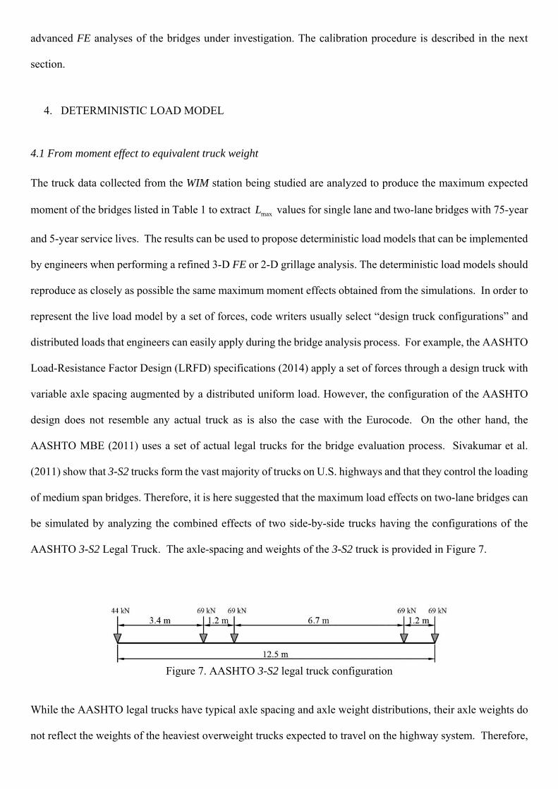
AASHTO 3-S2 Legal Truck. The axle-spacing and weights of the 3-S2 truck is provided in Figure 7.

Figure 7. AASHTO 3-S2 legal truck configuration

While the AASHTO legal trucks have typical axle spacing and axle weight distributions, their axle weights do

not reflect the weights of the heaviest overweight trucks expected to travel on the highway system. Therefore,

the goal of the calibration process is to propose a load model composed of trucks with typical configura-tions

but with axle weights that would produce mean load effect ( maxL ) values equal to those obtained by Equation

(6). For the analysis of short to medium span multi-girder bridges under single lane loadings, a single truck

would be applied. The analysis of multi-lane bridges requires the application of two-side-by-side trucks. How-

ever, as observed from actual WIM data, it is evident that the maximum load is due to the crossing of very heavy

trucks that may be either illegally overweight or have been issued permits. In any case, the simulations executed

in this study and other studies indicate that it is very unlikely that the maximum load is produced by side-by-

side trucks of equal weight. Actually, according to Trukstra’s (1980) well known reliability-based load combi-

nation rule, the maximum combined load effect can be approximately modeled by a maximum load expected

in one lane and a representative “point in time” load in the other lane. In this study, and for the sake of simpli-

fying the proposed live load model, it is suggested that the point-in-time load would be represented by a typical

truck carrying its legally permissible weight while the other truck carries sufficient overweight. The legal and

overweight trucks would be positioned on the bridge deck in a side-by-side configuration that reproduces the

maxL load effect value obtained from Equation (6).

It is observed that the variability of the maximum load effect for the entire population of steel composite

bridges and for the four most critical beams is quite low, with a coefficient of variation ranging from 4.5 % for

a time period of 75 years to a 5.6 %, for a time period of 5 years and for all beams. Therefore, even though the

calibration will be based on maxL , as the COV is relatively low, maxL is still very close to the highest possible

load that may cross the bridge. The variations of maxL around its mean value is accounted for through the

calibration of the live load safety factor as explained by Ghosn et al. (2013).

It is worth noting that Equation 6 gives the mean value of the maximum traffic effect in the service life

considered. While the analyses performed in this study assume a 75-year design life or 5-year rating period, a

similar approach can be followed if the desired result is to simulate the load effect corresponding to any speci-

fied return period such as the 1000-year return period used for the analysis of bridges following the Eurocodes.

The use of a pre-set return period is possible because Equations (4) through (7) provide all the statistical bases

to describe entire sets of Gumbel distributions for different service lives or return periods.Figure 8

Figure 8 shows the positioning of side-by-side legal trucks that would simulate the maximum load effect.

The figure introduces the parameter as a multiplier of the weight of the most eccentric truck such that the

maximum moment produced by the two side-by-side trucks of weights P and P on the most critical member

(longitudinal beam) is equal to the maximum traffic moment effect obtained from Equation 6 in the same mem-

ber.

Figure 8. Side-by-side truck loading pattern.

The analysis of the results shows that the parameter depends on the bridge configuration represented by

the three parameters of span length (SL), number of beams (NB) and beam spacing (BS). Some representative

results are shown in Figures 9 to 11 for the 5-year maximum load effect case. Figure 9 shows plots of the

parameter versus number of beams for spacings equal to 1.2 m, 1.8 m and 2.4 m for simple span bridges

with 30 m in length. Figure 10 plots versus the number of beams and span length for bridges with 1.8 m

beam spacing. Figure 11 shows the sensitivity of to beam spacing and span length for 6-beam bridges. These

plots are for the cases when the trucks take the configuration of the AASHTO 3-S2 Legal trucks.

Figure 9. Sensitivity of to number of beams and beam spacing for 30 m simply supported bridges.

Figure 10. Sensitivity of to number of beams and span length for bridges with 1.8 m of beam spacing.

Figure 11. Sensitivity of to beam spacing and span length for 6- beam bridges.

The figures demonstrate a clear difference in the behavior of shorter span bridges, with span-lengths less

than 30 m. This is due to the geometry of the 3-S2 truck. In fact, the truck’s full length is 12.5 m and bridges

with spans of similar span lengths are primarily controlled by single unit trucks rather than semi-trailer trucks.

On the other hand, the bridges with span length over 30 m present a parameter with more regular behavior.

As explained, 3-S2 type semi-trailers form the vast majority of trucks traveling on US highways and these trucks

produce the largest load effects on the main members of medium span bridges. On the other hand, Type 3 single

unit trucks, which also are frequently observed yet usually not dominant, control the loading on short span

bridges. Therefore, it is here suggested that the maximum load effects expected on single lane and two-lane

bridges can be simulated using either one Type 3, one 3-S-2, or the combined effects of two side-by-side trucks

having the configurations of either the AASHTO Type 3 or 3-S2 Legal Trucks with a modification factor applied

to a part of their weights to simulate the same effect of the traffic measurements.. Figure12 provides the con-

figuration of the AASHTO Type 3 Legal Truck.

Figure 12. AASHTO Type 3 Legal Truck configuration.

Referring to Figure 8, different values of the parameter may be obtained for the bending moments due to

one-lane and two-lane loadings depending on the transverse position of the two trucks. For this reason, the

worst loading conditions are considered regarding the transverse placement of the single or two side-by-side

trucks. The longitudinal position of the trucks to be employed and their configurations should be selected to

produce the highest value of the bending moment. The most critical positions are established separately for

each truck depending on the lane it occupies.

With the introduction of the new Type 3 truck, a new calibration of is carried out by equating the mean of

the maximum load effect produced by Equation (6) to the legal truck load effect using the following equation

for one-lane loading:

legalE

L

1

1max, (9)

For two-lane loadings, the parameter of the legal truck in the main drive lane is obtained according to the

following equation:

legal

legal

E

EL

1

22max, (10)

where kLmax, is the mean value of the maximum load effect obtained from Equation (6) over k traffic lanes,

and legaliE is the effect of the legal truck (3-S2 or Type 3) located in such a way as to produce the maximum

effect position in lane i .

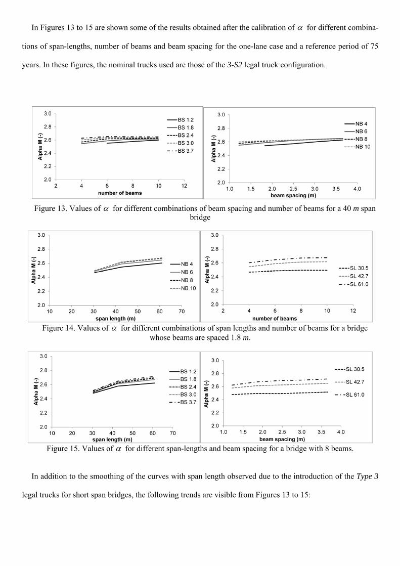
In Figures 13 to 15 are shown some of the results obtained after the calibration of for different combina-

tions of span-lengths, number of beams and beam spacing for the one-lane case and a reference period of 75

years. In these figures, the nominal trucks used are those of the 3-S2 legal truck configuration.

Figure 13. Values of for different combinations of beam spacing and number of beams for a 40 m span bridge

Figure 14. Values of for different combinations of span lengths and number of beams for a bridge

whose beams are spaced 1.8 m.

Figure 15. Values of for different span-lengths and beam spacing for a bridge with 8 beams.

In addition to the smoothing of the curves with span length observed due to the introduction of the Type 3

legal trucks for short span bridges, the following trends are visible from Figures 13 to 15:

a) Increasing the number of beams results in higher values of moment effects, but an asymptotic value is

reached at about 8 beams. This is because for wide bridges with many beams, the beams that are laterally too

far from the position of the trucks do not contribute much to carrying the applied load.

b) As the span length increases, the effect of the axle spacing decreases as actual trucks in the WIM database

and the proposed load model trucks tend to increasingly act as concentrated forces. Therefore, the parameter

asymptotically approaches a constant value as the span length increases. For the shorter spans, the AASHTO

Legal Truck’s short axle spacing compared to those of the actual semi-trailers and single unit trucks in the

traffic stream would lead to relatively higher load effects than those of the actual trucks. In those cases, the

change in the denominator of Equation (10) is always smaller than that of the numerator in Equations (9) and

(10).

c) The parameter is dependent on the span length and to a certain extent on the beam spacing as can be

observed in Figures 13 to 15. These changes in are due to the differences in the axle spacing and the per-

centage of weight carried by each axle of the nominal trucks compared to those of the actual trucks. In fact, the

lateral distribution of a point load to the different beams is related to the position of the load relative to the

bridge’s supports. Therefore, changes in the bridge length and the truck’s configuration would influence the

load distribution and subsequently affect the parameter .

Studying the results in the above listed figures, it may be convenient to summarize the calculated values of

the parameter into a single equation which, through a regression analysis, can take the form:

2

2

2

2

2

2

111.

68.15.30

68.15.30

NBc

BSb

SLa

NBc

BSb

SLaconsteq

(11)

where SL is the span length in meters, BS is the beam spacing in meters, NB is the number of beams, const

and 1a , 1b , 1c , 2a , 2b , 2c are coefficients calibrated to minimize the error in estimating a value of the parameter

.eq , The 7 coefficients are calibrated using the calculated parameter for all the bridges in the database by

minimizing the following mean error index:

toterr n

err (12)

.eqerr

(13)

where totn is the total number of bridges analyzed, in this case, 100. The six parameters 1a , 1b , 1c , 2a , 2b , 2c

are curve shape coefficients that depend on the load case (one or two side-by-side trucks) and the governing

truck type, while the coefficient const reflects the truck type that governs the loading process and the service

life.

The results of the minimization process are reported in Table 4. The values of those coefficients are similar for

the two cases of 5-year and 75-year maximum expected load. However, the value of const is different as

presented in table 5.

Table 4. Coefficients of Equation (11) for one-lane and two-lane loadings.

3-s2 Type 3

1 Lane 2 Lanes 1 Lane 2 Lanes

a1 0.263 0.380 1.828 1.378

b1 0.001 0.066 0.047 0.152

c1 0.245 0.178 0.908 0.273

a2 -0.086 -0.112 -0.074 -0.017

b2 0.001 -0.006 -0.016 -0.051

c2 -0.103 -0.059 -0.389 -0.113

Table 5. Value of the constant const of Equation (11) for different nominal truck and service lives.

M (1-lane) (3-S2) M (2-lane) (3-S2) M (1-lane) (Type 3) M (2-lane) (Type 3) 5 years 1.86  1.19  0.80 0.68 75 years 2.06  1.42  1.03 0.98 

The Type 3 coefficients are usually used for short spans (less than 30 m) where the size of the truck is com-

parable to the span length. However, when the procedure is applied for the analysis of a particular bridge, a

preliminary comparison between the effect of 3-S2 trucks and Type 3 trucks should be checked, and the most

critical considered.

5. IMPLEMENTATION

Two numerical examples are presented to illustrate how the proposed calibrated live load model can be used

in engineering practice to: (1) design new bridges; or more importantly, (2) perform more accurate evaluations

of deteriorating existing bridges than current simplified analysis procedures would produce.

5.1.Example 1: Design of a new bridge

Let us consider a 30 m span-length steel composite bridge, 12 m wide with 8 beams spaced at 1.8 m center

to center. The bridge is to be built close to the WIM station 9121 in the State of New York that was used to

calibrate the model described in this paper.

The moment due to the live-load on the most loaded beam calculated according to the standard procedure of

the AASHTO LRFD (2014) including the use of the load distribution factors gives a maximum moment equal

to 2315 kNm. in the most loaded beam. During the design process, this nominal live load moment is associated

with a live load factor 75.1L . This indicates that the factored live load should be equal to 4051 kNm. This

value can be used to design the beams of the bridge. However, tabulated load distribution factors represent a

wide range of bridges. Therefore, if the design engineer wants to use a more accurate value, he/she would need

a more accurate estimate of the traffic effects on this particular bridge. In this case, the engineer may choose to

use the proposed calibrated parameter to apply a more accurate live load model that can be used in combi-

nation with a grillage analysis of the bridge. The process consists of the following steps:

1. From Tables 4 and 5, the required coefficients to apply in Equation (11) are obtained according to the

bridge characteristics: beam spacing of 1.8 m, a span length equal to 30 m and 8 beams, resulting in a

parameter .eq equal to 1.88 for the two-lane case and 75-year service-life. This is contrasted to a value

of 2.38 for the one-lane loading. The different values reflect the lower probability of having an extremely

heavy truck crossing the bridge simultaneously with another truck as compared to having the extremely

heavy truck crossing the bridge on its own.

2. A system of forces representing two side-by-side trucks or a single truck having the configuration of the

AASHTO 3-S2 Legal Trucks are applied on a grillage model of the bridge to calculate the maximum

moment in the bridge beams. In the side-by-side case, the axle weights of one of the 3-S2 trucks are

multiplied by .eq =1.88, while the weights of the other truck are kept as shown in Figure 8. In the one-

lane loading case, the axle weights are multiplied by .eq =2.38. The worst position in the longitudinal

direction is found by varying the position of the system of trucks in the model until the maximum mo-

ment effect on the most critical longitudinal member is found. After including the dynamic effect, that

is set to be exactly equal to that obtained when using the AASHTO dynamic amplification, the total

moment on the exterior composite beam is found to be 2169 kNm for the side-by-side case, compared to

2151 kNm the one-lane case. It is interesting to observe that in this case, both the one and the two-lane

loading give very similar values for the maximum moment in the most loaded beam with the two-lane

case being very slightly higher.

3. During the calibration of the AASHTO LRFD, Nowak (1999) observed that the HL-93 load model pro-

duced load effects about 1.25 times lower than the maximum 75-year load effect obtained from the traffic

data. The AASHTO LRFD applies a live load factor 75.1LL to ensure that bridges analyzed using

the AASHTO LRFD produce a reliability index 50.3 . Because the parameter calculated in this

study is based on matching the expected 75-year maximum live load effect, then the factored live load

factor that should be used in designing the bridge members should be calculated as:

kNmkNmLLfac 3037216925.1

75.1 (14)

This proposed live load design moment is lower than the one obtained when using the AASHTO (2014)

design equations equal to 4051 kNm. The lower value reflects the improved accuracy of the live load model

and the analysis process performed using the proposed approach. The method can also consider the case where

due to the increase in the traffic loading during the years, the codified live-load model calibrated with existing

WIM data at the time of Code writing, may lead to unconservative results. In this case, Equation (14) will

provide the correct facLL to be used in the design.

5.2.Example 2: Rating of a deteriorated bridge

While designing bridges with lower load effects may lead to some savings, engineers would prefer to be on

the side of conservativeness and use traditional analysis and design procedures rather than use intricate analyses

procedures and new live load models. But the implementation of the approach proposed in this paper is most

interesting in the case of a refined analysis that engineers may resort to executing when rating existing bridges.

This is most relevant in the case of bridges that were designated as insufficiently safe when using traditional

methods or those that may be exposed to truck weights significantly different than the typical trucks which were

used during the calibration of the traditional procedures. For example, we consider that the same simply-sup-

ported composite steel 12 m wide steel girder bridge having a 30 m span-length, with 8 beams spaced at 1.8 m

center to center is to be rated for Strength I Inventory and Operating levels. Following the AASHTO MBE

manual (2011), Inventory Rating (IR) is executed under the effect of the HL-93 design load with a live load

factor 75.1LL while Operating Rating is executed using a live load factor 35.1LL . The rating equation

is given as:

IMLL

DWDCRF

LL

DWDCsc

(15)

where c is the condition factor set at 0.85 for a bridge in poor condition to account for the increased uncer-

tainties in assessing the strengths of its members. 00.1s is the system factor for an 8-beam bridge, 00.1

is the resistance factor for steel girders in bending. kNmRn 4850 is the nominal resistance as inspected of

one composite beam. 25.1DC is the LRFD load factor for structural components, kNmDC 1100 is the

dead load effect due to concrete deck and barriers on one beam plus 360 kNm for one steel beam self-weight

plus miscellaneous steel. 50.1DW is the LRFD load factor for wearing surface, kNmDW 243 is the dead

load effect on one composite steel beam due to wearing surface. Finally, 75.1LL or 35.1 are the evaluation

live load factors for the Inventory Rating Factor and Operating Rating Factor respectively, LL is the HL-93

live load effect, and LLIM 33.0 is the dynamic load allowance. Given that the design load effect including

the dynamic allowance as tabulated in the AASHTO MBE (2011) is kNmDC 3859 for a 30 m simple span

bridge, and after applying a distribution factor 60.0DF for the exterior beam, the live load on one beam is

kNmIMLL 2315 .

Substituting the above values in Equation (15) leads to an Inventory Rating Factor 58.0IR and an Operating

Rating Factor 76.0OR . The engineer decides not to apply Legal Load ratings because the bridge is along a

route that is exposed to large numbers of overweight trucks. Therefore, being less than 1.00, the calculated

inventory and operating RF factors are deemed unacceptable and the bridge should have been slated for re-

placement or major rehabilitation. Instead, the engineer decides to execute a site-specific evaluation of the

bridge using a refined analysis using the proposed approach which takes into consideration the WIM data col-

lected at New York station 9121 that is considered to be consistent with the trucks crossings the bridge. For the

inventory rating, the 75-year maximum moment and for the operating rating the 5-year maximum are respec-

tively used. Using the coefficients in Tables 4 and 5 and after including the dynamic effect, IM, which in this

case is assumed to have the same value as that obtained when using the AASHTO dynamic effect, the maximum

75-year moment for inventory rating is found to be equal to 2169 kNm, and the 5-year moment used for oper-

ating rating is 1970 kNm. These values are implemented in the denominator of Equation (15) but because they

are based on actual projections of the maximum load effects and not on nominal live load models, the live load

factor in the denominator is changed to LL 1.75/1.25 or 1.35/1.25 for the Inventory and Operating ratings

respectively. Substituting these adjusted live loads and associated live load factors gives the corresponding

rating factors of 0.78 and 1.11 for inventory and operating ratings. Thus, the adjusted operating rating is above

1.00 and the bridge is assumed to have sufficiently levels of safety over the short-term to sustain the expected

traffic loads even if the traffic includes overweight vehicles.

As seen in the above examples, the definition of the live load models as presented in the AASHTO specifi-

cations may be conservative for the design and evaluation of bridges are performed following current simplified

analysis that are based on simple beam models in conjunction with tabulated load distribution factors. The

proposed calibration of live load models for use with more advanced deterministic analyses will produce more

accurate results. Thus, the proposed approach may in many cases lead to saving some bridges that may not

traditionally rate well from immediate replacement or rehabilitation and may lead to a more efficient allocation

of the limited resources currently available for managing our ageing bridge infrastructure. Additional work to

extend the procedure proposed in this paper to cover different sets of WIM data and for the analysis of moment

and shear effects on a wider range of bridge configurations is described by Anitori et al. (2017).

When an advanced reliability analysis is to be performed, modeling the effects of heavy trucks on bridges

must include additional statistical parameters to fully define the random nature of the applied live loads. The

procedure developed in this paper will also provide statistical models to consider the uncertainties and variabil-

ity in the proposed live load model (Anitori et al., 2017).

6. CONCLUSIONS

A method is presented to calibrate a deterministic live load model that can be used to perform refined FE

and grillage analyses for the design or evaluation of composite steel simply-supported multi-girder bridges. The

significance of the proposed live-load model derives from its capability of producing more accurate results

during FE analysis of bridges than code-specified load models that are calibrated for use in combination with

simplified analysis methods that utilize tabulated load distribution factors. Such calibrated live load models are

not only valid for application during standard design and safety evaluation processes based on a linear-elastic

behavior, but also when a non-linear analysis of the bridge system, which considers internal force redistribution

among the bridge elements, is foreseen. Using live load models calibrated using the proposed procedure will

better simulate the effects of actual vehicular traffic.

Two examples are presented to show the benefits of the proposed method when more accurate results than

those obtained using the standard design and/or assessment procedures are needed by the engineer in order to

make appropriate decisions on bridge maintenance and replacement needs.

The live load calibration process is presented in this paper for the case of bending moments in composite

steel multi-girder bridges. The same approach can be used to develop live-load models suitable for other bridge

types and load effects. Also, the same approach can be followed to calibrate live load models representing truck

traffic in different regions or for application when using different codes and standards such as the AASHTO

specifications or the Eurocodes, provided that WIM data from the appropriate regions are available.

It was found that in the case of traffic data collected at a typical site in upstate New York, the AASHTO 3-

S2 Legal Truck can provide an acceptable live load pattern for simulating the maximum bending moment effect

in the case of medium span bridges with span lengths in the range from 30 to 60 m. However, for short spans,

the AASHTO Type 3 legal truck gives better results. This trend should be further confirmed through the analysis

of traffic from other WIM stations in the U.S. and also for other traffic load effects as, for instance, shear.

The results presented in this paper are based on the traffic data from only one specific WIM station. The

same methodology can be applied to a set of WIM stations in a specific region, state or country to develop

specific amplification factors and live-load models, as presented in Anitori et al. (2017). Furthermore, the cali-

bration process provides information on site-to-site variability to calibrate different models for different traffic

characteristics.

Even though live-load models derived using the procedure described in this paper would be readily applica-

ble for performing deterministic design/assessment analyses, the models can be easily extended to propose

probabilistic-based live load models as more data from other WIM stations are made available. In this way, the

traffic model can be used in combination with a reliability-based analysis of bridge systems as presented in

Anitori et al. (2017).

ACKNOWLEDGMENTS

The authors would like to thank the Spanish Ministry of Economy and Competitiveness (MINECO) and the

European Regional Development Funds (FEDER) for the financial support provided through projects BIA2010-

16332, BIA2013-47290-R and REHABCAR (INNPACTO). The third author also appreciates the financial

support from the Spanish Ministry of Education through the project SAB2009-0164 that provided funding dur-

ing his Fellowship stay at the Technical University of Catalonia.

REFERENCES

AASHTO (American Association of State Highway and Transportation Officials). (2011). The manual for

bridge evaluation : 2014 interim revisions, Washington, DC

AASHTO (American Association of State Highway and Transportation Officials). (2014). Bridge design

specifications. AASHTO LRFD, Washington, DC.

AASHTO (American Association of State Highway and Transportation Officials). (1996). Standard Speci-

fications for Highway Bridges, Washington, DC.

Ang, A.H.S. & Tang, W. H. (2007). Probability concepts in engineering : emphasis on applications in civil

& environmental engineering. New York: Wiley.

Anitori, G., Casas, J.R. & Ghosn, M. (2016). Live Load Model for Refined Analysis of Short and Medium-

span Bridge Systems. Proceedings of IABMAS-2016. Foz do Iguaçu (Brasil).

Anitori, G., Casas, J.R. & Ghosn, M. (2017). WIM based Live Load Model for Advanced Analysis of Simply

Supported Short and Medium-Span Highway Bridges. Journal of Bridge Engineering (ASCE). 22(10)

CEN (2002). EN 1991-2: Actions on Structures. Part 2: traffic loads on bridges.” Eurocode 1,. European

Committee for Standardization, Brussels.

Canadian Standards Association (CSA), (2014). S6-14 Canadian Highway Bridge Design Code. Canadian

Standards Association, 5060 Spectrum Way, Suite 100, Mississauga, Ontario, Canada.

Fiorillo, G. & Ghosn, M. (2014). Procedure for Statistical Categorization of Overweight Vehicles in a WIM

Database. Journal of Transportation Engineering, doi: 10.1061/(ASCE)TE.1943-5436.0000655.

Fiorillo, G., (2015) "Reliability and Risk Analysis of Bridge Networks under the Effect of Highway Traffic

Load", Dissertation presented in partial fulfillement for the requirements for a Ph.D., Department of Civil

Engineering. The City College of New York/CUNY, New York.

Fu,G. Liu,L. & Bowman, M.D. (2013). Multiple Presence Factor for Truck Load on Highway Bridges. Jour-

nal of Bridge Engineering (ASCE), 18(3), 240-249

Ghasemi, S.H., Nowak, A. S. & Hossein, P. (2016). Statistical Parameters of In-A-Lane Multiple Truck

Presence and a New Procedure to Analyze the Lifetime of Bridges. Structural Engineering International, 26

(2), 150-159

Ghosn, M. & Sivakumar, B. (2010). Using Weigh-In-Motion Data for Modeling Maximum Live Load Effects

on Highway Bridges. Proceedings of IABMAS-2010. Philadelphia (USA)

Ghosn, M., Sivakumar, B. & Miao, F. (2011). Load and Resistance Factor Rating (LRFR) in NYS. New

York: The City University of New York.

Ghosn, M., Sivakumar, B., & Miao, F. (2013). Development of State-Specific Load and Resistance Factor

Rating Method. Journal of Bridge Engineering (ASCE), 18(5), 351–36

Ghosn, M., Fiorillo, G., Gayovyy, V., Getso, T., Ahmed, S.& Parker, N. (2015). Effects of Overweight

Vehicles on New York State. DOT Infrastructure Final Report; Research Study No. C-08-13. Albany, NY,

USA.

Hambly, E. C. (1991). Bridge deck behaviour, London, E. & F.N. Spon.

Leahy, C., OBrien, E. J., Enright, B. & Hajializadeh, D. (2015). Review of HL-93 Bridge Traffic Load Model

Using an Extensive WIM Database. Journal of Bridge Engineering (ASCE), doi: 10.1061/(ASCE)BE.1943-

5592.0000729.

Moses, F. (2001). Calibration of load factors for LRFR bridge evaluation. Washington, D.C.: National

Academy Press

Nowak, A. S. (1999). Calibration of LRFD Bridge Design Code. Washington, D.C.: National Academy

Press

OBrien, E. & Enright, B. (2011). Modeling same-direction two-lane traffic for bridge loading. Structural

Safety, 33 (4-5): 296-304

Pelphrey, J., Higgins, C., Sivakumar, B., Groff, R. L., Hartman, B. H., Charbonneau, J. P., Rooper, J. W.,

Johnson, B. V. (2008). State-Specific LRFR Live Load Factors Using Weigh-in-Motion Data. Journal of Bridge

Engineering, doi: 10.1061/(ASCE)1084-0702(2008)13:4(339).

Sivakumar, B., Ghosn, M. & Moses, F. (2011). Protocols for Collecting and Using Traffic Data in Bridge

Design. NCHRP Report n.683. Transportation Research Board, National Research Council. Washington D.C.:

National Academy Press.

Soriano, M., Casas, J. R. & Ghosn, M. (2014). Simplified probabilistic model for maximum traffic load from

weigh-in-motion data. Procedings of IABMAS-2014. Shanghai (China).

Soriano, M., Casas, J. R. & Ghosn, M. (2016). Simplified probabilistic model for maximum traffic load from

weigh-in-motion data. Structure and Infrastructure Engineering, 13(4), 454-467, doi:

10.1080/15732479.2016.1164728.

Trukstra, C.J.& Madsen, H.O. (1980). Load combinations in codified structural design, ASCE Journal of

Structural Engineering, 106 (12), 2527–2543.

Zokaie, T., Mish, K. D., & Imbsen, R. A. (1995). Distribution of wheel loads on highway bridges, phase 3.

NCHRP 12-26/2 Final Report, Transportation Research Board, National Research Council. Washington D.C.:

National Academy Press.