Methodologies for Successful Segmentation of HRTEM Images via Neural Network

Catherine K. Groschner and Christina ChoiDepartment of Materials Science and Engineering,

University of California Berkeley, Berkeley, CA 94720

M. C. Scott∗

Department of Materials Science and Engineering,University of California Berkeley, Berkeley, CA 94720 and

Molecular Foundry, Lawrence Berkeley National Laboratory, Berkeley, CA 94720†

High throughput analysis of samples has been a topic increasingly discussed in both light andelectron microscopy. Deep learning can help implement high throughput analysis by segmentingimages in a pixel-by-pixel fashion and classifying these regions. However, to date, relatively littlehas been done in the realm of automated high resolution transmission electron microscopy (HRTEM)micrograph analysis. Neural networks for HRTEM have, so far, focused on identification of singleatomic columns in single materials systems. For true high throughput analysis, networks will needto not only recognize atomic columns but also segment out regions of interest from background fora wide variety of materials. We therefore analyze the requirements for achieving a high performanceconvolutional neural network for segmentation of nanoparticle regions from amorphous carbon inHRTEM images. We also examine how to achieve generalizability of the neural network to a range ofmaterials. We find that networks trained on micrographs of a single material system result in worsesegmentation outcomes than one which is trained on a variety of materials’ micrographs. Our finalnetwork is able to segment nanoparticle regions from amorphous background with 91% pixelwiseaccuracy.

I. INTRODUCTION

The last decade has seen a huge push in highthroughput materials discovery. A portion of thishas been the Materials Project, which provides highthroughput computations of material properties [1].Similarly, other high throughput materials discoveryefforts have also created a need for automated structuralvalidation which can be used in a high throughputmanner [2–4]. This is particularly apparent in thearea of high throughput nanomaterial design andsynthesis, where microstructural features, such asnanoparticle size and shape or the presence of grainboundaries and crystal defects, can strongly influence thematerial’s properties [5–8]. Additionally, heterogeneityin these microstructural features within populations ofnanomaterials will have observable effects on the bulkbehavior [6, 7, 9]. Therefore, a means of automatedatomic structure characterization is required to completethe high throughput materials discovery process. Inaddition, one could imagine that automating theatomic resolution segmentation task could be extremelyinfluential in enabling studies of the heterogeneity ofnanoparticle populations, an area which has been outof reach.

Electron microscopy is the only technique which canenable the analysis of local atomic-scale structure andaccount for structural heterogeneity. Techniques suchas X-ray diffraction may provide precise crystallographic

∗ Corresponding author† mary.scott@berkeley.edu

information, but only by averaging over the structureof thousands of particles. Electron microscopy istherefore the method of choice to identify local,atomic-scale structural features. However, large scaleinformation extraction from electron micrographs is oftenprohibitively time consuming. Simple tasks such asparticle size and shape classification can be difficult andand are often performed manually [10]. While automatedidentification of local structures is possible [11, 12], itis challenging, time consuming, and sample-dependent,resulting in a constraint on the number of particles andnumber of samples analyzed. The sample-dependenceof previous techniques is a particularly importantlimitation towards fully automated characterizationwith HRTEM. Because the sample will determinethe amount of scattering and therefore the contrastbetween nanoparticle and background, methods thatrely solely on thresholding may fail unpredictably whenbroadly applied. Here we demonstrate a methodfor transferable, automated identification of metallicnanoparticle structures from HRTEM, which relies notonly on changes in contrast, but on the high-resolutionlattice texture in the nanoparticles themselves. Givenrecent advances in image interpretation using deeplearning [13, 14], segmentation via convolutional neuralnet (CNN) is a promising route towards automaticinterpretation of HRTEM micrographs.

To date, most work on segmentation of TEM imageshas been applied to biological samples and cryo-electronmicroscopy [15, 16]. However, the different lengthscales involved in these imaging modalities mean thatdetection can largely revolve around edge detectionand be dependent on mass and thickness contrast.

arX

iv:2

001.

0502

2v1

[ee

ss.I

V]

14

Jan

2020

2

High resolution imaging for materials science samplesare dependent on much different contrast mechanisms;predominately phase contrast which can result in highlynonlinear images [17]. Due to the image not beinga simple projection of atomic potentials, previouslyimplemented particle detection methods are not expectedto be effective.

Only recently has there been work on segmentationof HRTEM and high resolution scanning transmissionelectron microscopy (HRSTEM). The application ofCNNs to HRSTEM data has focused primarily onidentifying atoms in sheets of material filling the entirefield of view or in the prediction of atomic columnthickness or specific atom tracking [18–23]. Most workin this area has focused on atomic column finding inHRSTEM images, for example atom finding on largegraphene sheets in HRSTEM data to identify defects [18][20]. This approach has also been applied to HRSTEM insitu movies of WS2 [21]. While most of these works focuson a thin film which fills the field of view, recent workhas identified atomic columns belonging to a grapheneregion surrounded by amorphous carbon [24]. Less workhas been done in the area of HRTEM but what has beendone has also focused on atomic column finding, withapplications in strain and thickness measurement [19].Particle finding algorithms have been implemented, buthave not been sensitive to local atomic structure [25], andthe issue of generalizability has not been addressed.

We have focused on HRTEM as opposed to HRSTEMas it is a more dose-efficient imaging mode and thereforeuseful for a wider range of materials. However,segmentation in HRTEM is particularly challengingbecause the contrast between the substrate that thenanomaterial sits on and the nanomaterial itself canbe very low. Because traditional image processingtechniques are highly error prone for these types ofimages, we have implemented a convolutional neuralnetwork to handle semantic segmentation, which issegmentation of the image on a pixel by pixel basis.Neural network based semantic segmentation has theadded benefit of giving a confidence of prediction foreach pixel. We are particularly interested in segmentingout nanoparticle regions as opposed to individual atomiccolumns because then larger structural features andrelationships between atomic columns can be analyzedon a particle by particle basis. For example, thesesegmented regions can then be passed to other classifiersand techniques for various structural analysis such asclassifying nanoparticles containing dislocations. We useCNNs specifically because they have the flexibility togeneralize across samples and the speed to be used inother methods such as in-situ particle tracking.

Here we present a solution to nanoparticle regionidentification in HRTEM that performs well onnanoparticles with a wide range of compositions andtherefore scattering intensities. We have explored theimpact of training set on segmentation by analyzingthe results of three separately trained networks. We

have found that networks trained only on micrographsof highly scattering samples or lightly scattering samplesare not as robust as those which see a more diversedataset. We show that the more diverse dataset increasespixelwise segmentation accuracy and dice coefficient foreach individual dataset over networks trained to eachspecific dataset. These results point to a means ofachieving segmentation on a wide variety of nanoparticlesamples. This is likely due to the sensitivity of theneural network to lattice features. Our best performingCNN is able to segment nanoparticles with a 91%pixelwise accuracy. We were able to train this neuralnetwork using only 129 512x512 micrographs throughdata augmentation. The neural network is shown tobe robust to changes in contrast and is sensitive tothe presence of atomic columns. We confirm thisatomic column sensitivity by analyzing the activationmaps from the neural network. Taken as a whole,this represents a critical step to an automated imaging,particle identification, and structure analysis workflowfor nanoparticles.

II. METHODS

The overall goal of this work was to achieveaccurate segmentation on micrographs of 2 nm CdSenanoparticles. These samples were particularlychallenging because of the relatively low electronscattering from the low atomic number sample. Datasetsof CdSe nanoparticles and Au nanoparticles wereacquired in order to test the neural network’s sensitivityto changes in contrast, due to the change in scatteringpotential of the different materials. CdSe micrographsprovided a low scattering potential case while theAu nanoparticles were in the high scattering potentialregime. Three separate neural networks were trained.The first was trained using only Au data, the secondusing only CdSe data, and the third was trained usinga combination of both. Each time the network wasonly trained using 129 images in total. These threecases allowed us to test whether training would be moresuccessful on narrower tasks, such as identifying a singlematerial, or whether a greater diversity of images wouldimprove results. Micrographs of a completely differentmaterial system, Pd nanoparticles, were not used intraining but were used to test the generalizability of thenetwork to different materials.

A. Sample Preparation and Data Collection

We collected CdSe micrographs using the TEAM 0.5aberration corrected microscope at an operating voltageof 300 kV. CdSe particles were synthesized via theWANDA synthesis robot at the Molecular Foundry [5].This solution was then diluted with hexane and dropcaston 200 mesh ultra-thin carbon grids. Forty six 1024x1024

3

images were taken by hand. Labels for this datasetwere manually created using the MATLAB labeler app[26]. The CdSe particles being smaller and a loweratomic number material provided a lower contrast and,therefore, lower signal to background dataset.

Au nanoparticle data was collected using an FEIThemis with image aberration correction operated at 300kV. Au nanoparticles in phosphate buffered saline werepurchased from Sigma Aldrich. The Au nanoparticlesolution was diluted with water and dropcast onto 200 mesh carbon grids. Prior to drop casting,carbon grids were cleaned using a plasma cleaner.Thirteen 4026x4026 TEM micrographs were collectedusing SerialEM. SerialEM is a software which enablesautomated electron microscopy imaging [27], and wasused for automated focusing in order to speed up imagecollection. The autofocusing function also helped ensurethat the range of defocus was within approximately 100nm of Gaussian focus. Labels for network training werecreated by hand using the MATLAB labeler application[26].

Palladium nanoparticles were synthesized by a solutionmethod developed by Lim et al. [28]. 2 µL of the purifiedsolution was then dropcast onto a 200 mesh carbon grid.Prior to dropcasting the carbon grids were cleaned usinga plasma cleaner. The nanoparticles were then imagedusing a FEI Themis with image aberration correctionoperated at 300kV.

B. Data Preprocessing

After data collection, there were several key steps indata preprocessing. For the segmentation, two classeswere used: the nanoparticle class and the backgroundclass. Any contiguous crystalline region was labelled asbeing part of the nanoparticle class. All other regionswere labelled as carbon background. Should there havebeen contamination a third class would have been needed,but in this case clean enough samples were prepared forthis to not be necessary.

Images collected were 4096x4096 or 1024x1024 inInt16 format. Since large images make segmentationsignificantly more computationally demanding, we slicedeach image and its ground truth segmentation mapinto 512x512 images which remained in Int16 format.Keeping data in Int16 format was found to be crucialas converting to Int8 (as would be found in standardpngs) negatively impacted network training due to thelimited the dynamic range typical of HRTEM images.We used the openNCEM Python package in combinationwith custom code to for the image preprocessing [29].OpenNCEM was used for reading the mrc files producedby the microscope software into Python. Opened mrcfiles were then matched with the png label files so thatboth could be put into numpy arrays and saved as h5files. Once data had been properly sorted, both imagesand labels were sliced into 512x512 chunks and put into

an array. All the images were then normalized by firstapplying a median filter with a 3x3 kernel which servedto remove spurious X-rays. After filtering, the imageswere normalized by the filtered dataset maximum.

Significant portions of the raw input images werecarbon background, which meant that when slicedinto 512x512 images only 28% of images containednanoparticles. Since a class must be predicted foreach pixel, having only 28% of images contain particlesmeant that the background class was drastically overrepresented in the training, validation, and test set[30]. Therefore, we implemented a rough balancing ofclasses by using the ground truth segmentation maps todetermine which 512x512 images contained any pixelsbelonging to the particle class. Any image that didnot contain particle class pixels was discarded from thetraining and test set. For each network, 97 images wereused in the training set, 32 images were in the validationset, and 46 images were in the test set.

C. Network Training

For this experiment, three separate neural networkswere trained. One was trained solely on Au nanoparticledata, while the second was trained only on CdSe data.The third was trained on a combination of Au and CdSedata. The number of images used for training remainedconsistent for all three networks.

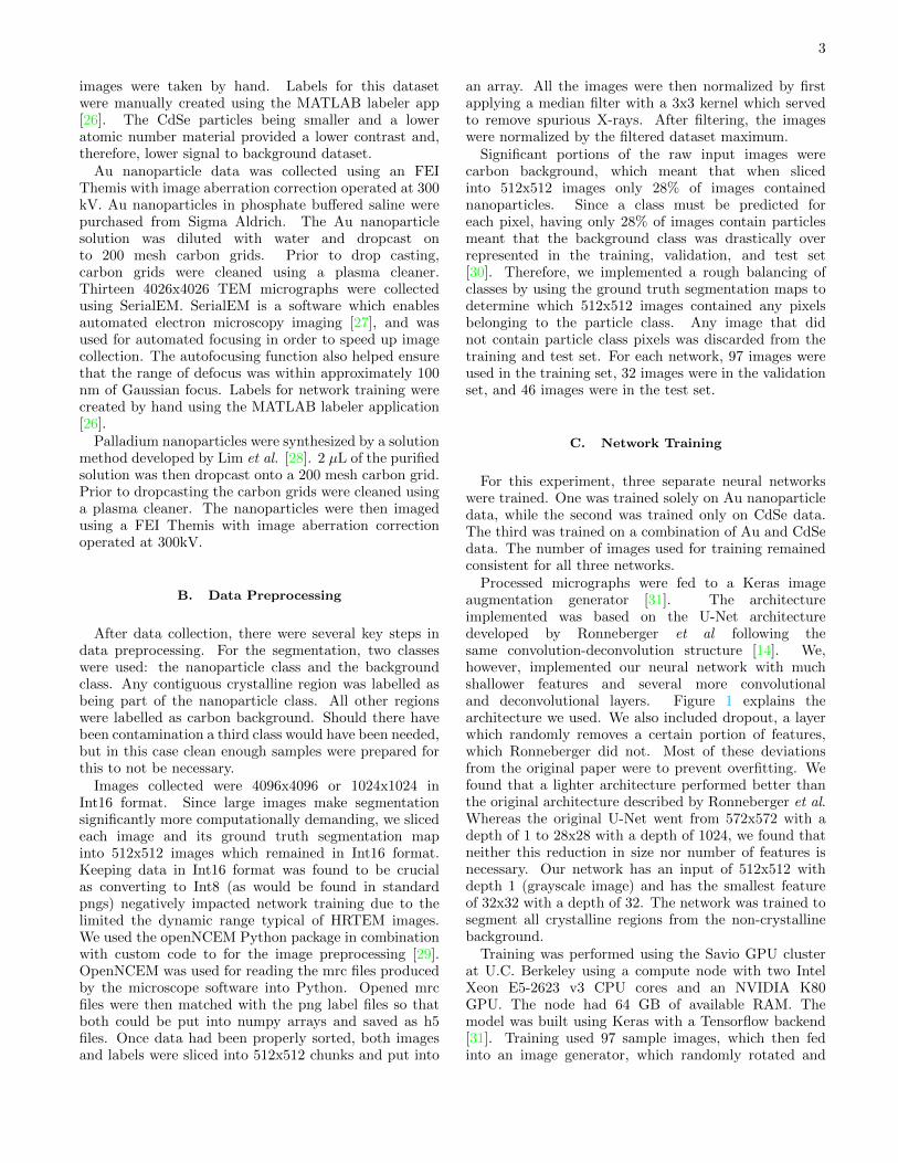
Processed micrographs were fed to a Keras imageaugmentation generator [31]. The architectureimplemented was based on the U-Net architecturedeveloped by Ronneberger et al following thesame convolution-deconvolution structure [14]. We,however, implemented our neural network with muchshallower features and several more convolutionaland deconvolutional layers. Figure 1 explains thearchitecture we used. We also included dropout, a layerwhich randomly removes a certain portion of features,which Ronneberger did not. Most of these deviationsfrom the original paper were to prevent overfitting. Wefound that a lighter architecture performed better thanthe original architecture described by Ronneberger et al.Whereas the original U-Net went from 572x572 with adepth of 1 to 28x28 with a depth of 1024, we found thatneither this reduction in size nor number of features isnecessary. Our network has an input of 512x512 withdepth 1 (grayscale image) and has the smallest featureof 32x32 with a depth of 32. The network was trained tosegment all crystalline regions from the non-crystallinebackground.

Training was performed using the Savio GPU clusterat U.C. Berkeley using a compute node with two IntelXeon E5-2623 v3 CPU cores and an NVIDIA K80GPU. The node had 64 GB of available RAM. Themodel was built using Keras with a Tensorflow backend[31]. Training used 97 sample images, which then fedinto an image generator, which randomly rotated and

4

FIG. 1. The U-Net style architecture of CNN implemented for segmentation of nanoparticle regions. Layers colored grayrepresent the output features and are labeled with the number of features created. Layers A-D contain a 2D convolutionallayer, batch normalization layer, ReLu activation layer, and a 2D max pooling layer. Layer E contains a 2D convolutionallayer, batch normalization layer, and ReLu activation layer, which is repeated once. Layers F-I contain a 2D upsampling layer,concatenation layer, a 2D convolution, batch normalization, and ReLu activation followed by a dropout layer and another setof 2D convolution, batch normalization, and ReLu activation layers. The final layer is a sigmoid activation layer which outputstwo segmentation maps one for each class, background and particle.

flipped the images. The only augmentations allowedwere rotations from 0-360 degrees, and mirroring. Eachepoch contained 1,000 samples created from rotating theoriginal processed 97 micrographs. Early stopping wasimplemented such that validation loss did not improvemore than 0.001 after two epochs. The model waslimited to train for a maximum of ten epochs. Themodel used categorical cross entropy for the loss functionand Adam as the optimizer with a learning rate was1x10−4 [32, 33]. Batch size was set to 20. The modelwas updated based on the results of a validation setcontaining 32 images. Training was done independentlyfor each different dataset.

D. Multiclass to Binary Classification

Despite only having two classes, we chose to treat thisproblem as a multiclass classification problem. Instead ofhaving the neural network output a single segmentationmap, which classifies the particle regions as 1 and thebackground as 0, we have it predict a segmentation mapfor both the background and particle class, as can be

seen in the final output shown in Figure 1. We foundthat this lead to better learning of the background classand therefore better end segmentation. This was evidentby the decrease in the number of false positives whenthe neural network predicted two separate segmentationmaps, one for each class.

Since the output of the neural network is two separatesegmentation maps, we must choose one for the finalsegmentation of pixels. For most training instances,the segmentation map for the particle class was moreconfident in its predictions for each pixel and yieldedhigher accuracy. Therefore, the final segmentation mapswhere based on thresholding the particle segmentationmap. The threshold was set to optimize pixelwiseaccuracy on the training data.

E. Testing

A holdout test dataset was reserved for final testingafter model training had completed. This test set isseparate from the vaildation set used during training.It consisted of 46 images. The model predicted

5

segmentation maps for both the background and particleclass of the test set. The final segmentation map wasthen taken from the particle segmentation map, whichwas then thresholded based on the previously determinedthreshold, as described above. Pixelwise accuracy valuesand dice coefficients were then calculated based on thesethresholded segmentation maps.

III. RESULTS AND DISCUSSION

We tested whether networks trained on the samenanoparticle material datasets could perform better ontheir specific dataset than on a network which had beentrained on a combination dataset. This was to testwhether networks would need to be trained for individualmaterial cases. Sample materials were hypothesizedto influence neural network performance due to thedependence of image contrast on the scattering potentialof the material. Overall, we found that a more diversefeature space created by training on a combinationdataset actually improved segmentation results for boththe Au and CdSe datasets. Finally, we also tested thegeneralizability of the combination network by having itsegment a micrograph of Pd allowing us to test how thenetwork responded on a new material system, under avariety of imaging conditions.

A. Results from Training with Gold NanoparticleMicrographs

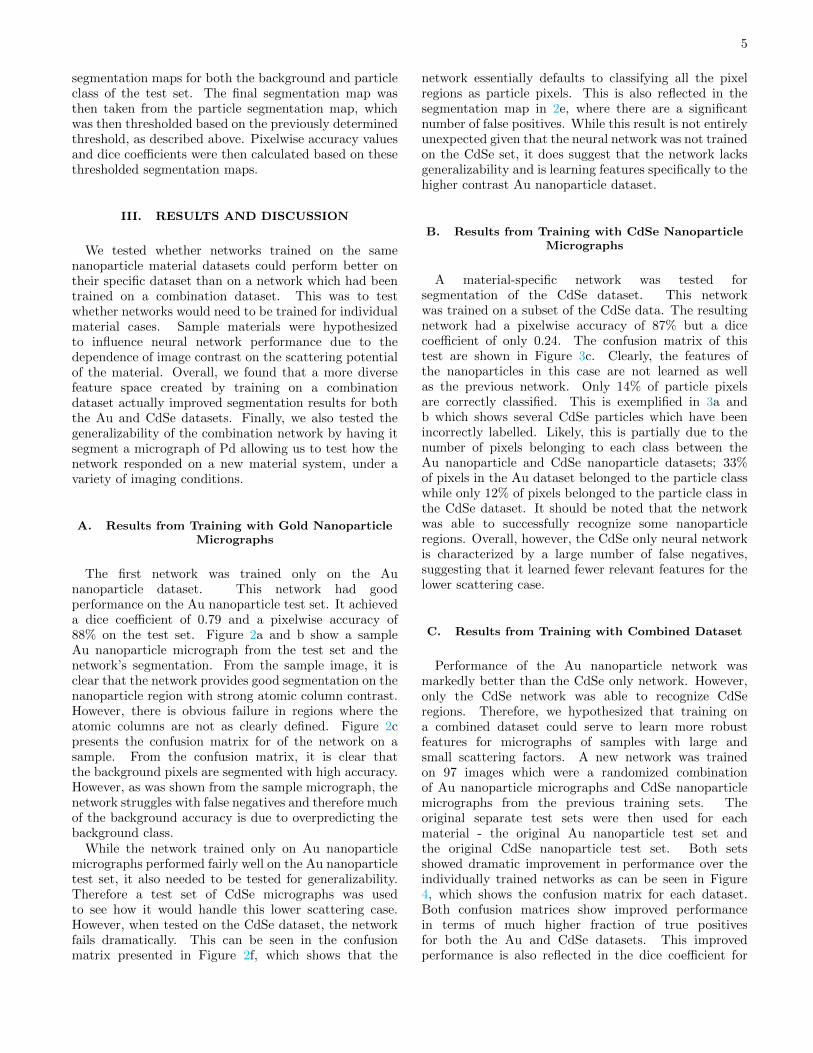
The first network was trained only on the Aunanoparticle dataset. This network had goodperformance on the Au nanoparticle test set. It achieveda dice coefficient of 0.79 and a pixelwise accuracy of88% on the test set. Figure 2a and b show a sampleAu nanoparticle micrograph from the test set and thenetwork’s segmentation. From the sample image, it isclear that the network provides good segmentation on thenanoparticle region with strong atomic column contrast.However, there is obvious failure in regions where theatomic columns are not as clearly defined. Figure 2cpresents the confusion matrix for of the network on asample. From the confusion matrix, it is clear thatthe background pixels are segmented with high accuracy.However, as was shown from the sample micrograph, thenetwork struggles with false negatives and therefore muchof the background accuracy is due to overpredicting thebackground class.

While the network trained only on Au nanoparticlemicrographs performed fairly well on the Au nanoparticletest set, it also needed to be tested for generalizability.Therefore a test set of CdSe micrographs was usedto see how it would handle this lower scattering case.However, when tested on the CdSe dataset, the networkfails dramatically. This can be seen in the confusionmatrix presented in Figure 2f, which shows that the

network essentially defaults to classifying all the pixelregions as particle pixels. This is also reflected in thesegmentation map in 2e, where there are a significantnumber of false positives. While this result is not entirelyunexpected given that the neural network was not trainedon the CdSe set, it does suggest that the network lacksgeneralizability and is learning features specifically to thehigher contrast Au nanoparticle dataset.

B. Results from Training with CdSe NanoparticleMicrographs

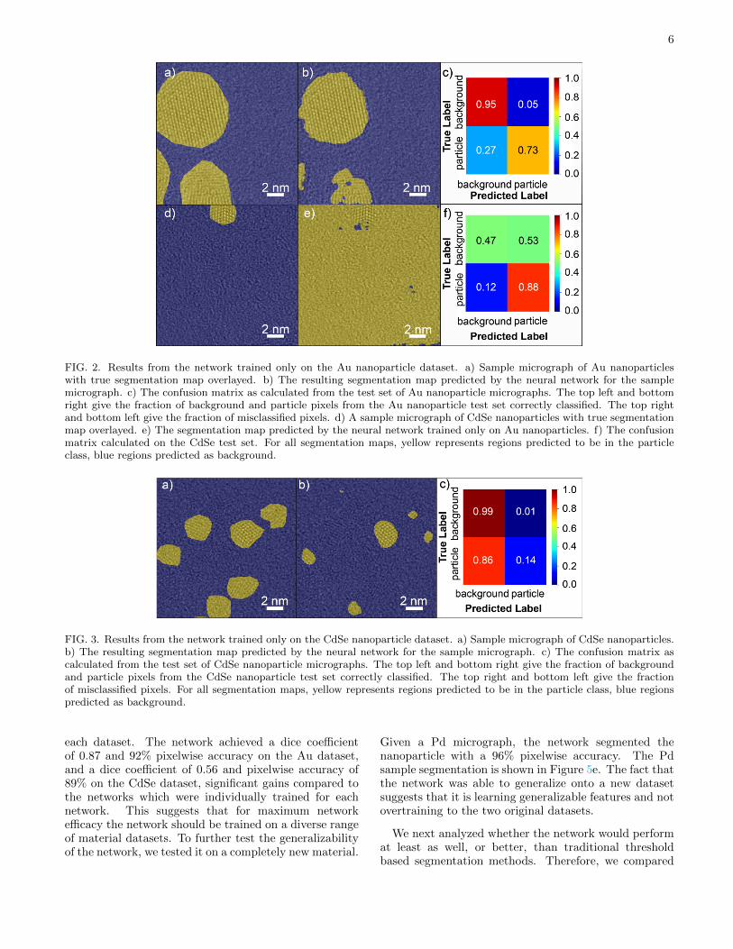
A material-specific network was tested forsegmentation of the CdSe dataset. This networkwas trained on a subset of the CdSe data. The resultingnetwork had a pixelwise accuracy of 87% but a dicecoefficient of only 0.24. The confusion matrix of thistest are shown in Figure 3c. Clearly, the features ofthe nanoparticles in this case are not learned as wellas the previous network. Only 14% of particle pixelsare correctly classified. This is exemplified in 3a andb which shows several CdSe particles which have beenincorrectly labelled. Likely, this is partially due to thenumber of pixels belonging to each class between theAu nanoparticle and CdSe nanoparticle datasets; 33%of pixels in the Au dataset belonged to the particle classwhile only 12% of pixels belonged to the particle class inthe CdSe dataset. It should be noted that the networkwas able to successfully recognize some nanoparticleregions. Overall, however, the CdSe only neural networkis characterized by a large number of false negatives,suggesting that it learned fewer relevant features for thelower scattering case.

C. Results from Training with Combined Dataset

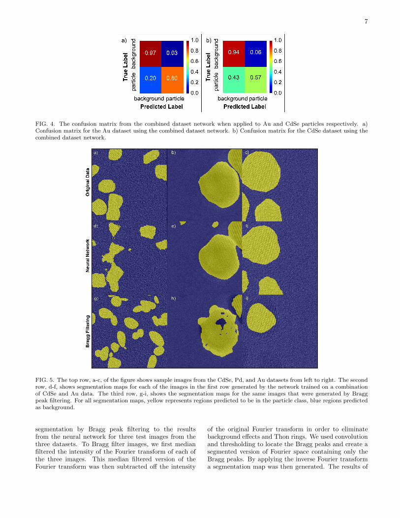
Performance of the Au nanoparticle network wasmarkedly better than the CdSe only network. However,only the CdSe network was able to recognize CdSeregions. Therefore, we hypothesized that training ona combined dataset could serve to learn more robustfeatures for micrographs of samples with large andsmall scattering factors. A new network was trainedon 97 images which were a randomized combinationof Au nanoparticle micrographs and CdSe nanoparticlemicrographs from the previous training sets. Theoriginal separate test sets were then used for eachmaterial - the original Au nanoparticle test set andthe original CdSe nanoparticle test set. Both setsshowed dramatic improvement in performance over theindividually trained networks as can be seen in Figure4, which shows the confusion matrix for each dataset.Both confusion matrices show improved performancein terms of much higher fraction of true positivesfor both the Au and CdSe datasets. This improvedperformance is also reflected in the dice coefficient for

6

FIG. 2. Results from the network trained only on the Au nanoparticle dataset. a) Sample micrograph of Au nanoparticleswith true segmentation map overlayed. b) The resulting segmentation map predicted by the neural network for the samplemicrograph. c) The confusion matrix as calculated from the test set of Au nanoparticle micrographs. The top left and bottomright give the fraction of background and particle pixels from the Au nanoparticle test set correctly classified. The top rightand bottom left give the fraction of misclassified pixels. d) A sample micrograph of CdSe nanoparticles with true segmentationmap overlayed. e) The segmentation map predicted by the neural network trained only on Au nanoparticles. f) The confusionmatrix calculated on the CdSe test set. For all segmentation maps, yellow represents regions predicted to be in the particleclass, blue regions predicted as background.

FIG. 3. Results from the network trained only on the CdSe nanoparticle dataset. a) Sample micrograph of CdSe nanoparticles.b) The resulting segmentation map predicted by the neural network for the sample micrograph. c) The confusion matrix ascalculated from the test set of CdSe nanoparticle micrographs. The top left and bottom right give the fraction of backgroundand particle pixels from the CdSe nanoparticle test set correctly classified. The top right and bottom left give the fractionof misclassified pixels. For all segmentation maps, yellow represents regions predicted to be in the particle class, blue regionspredicted as background.

each dataset. The network achieved a dice coefficientof 0.87 and 92% pixelwise accuracy on the Au dataset,and a dice coefficient of 0.56 and pixelwise accuracy of89% on the CdSe dataset, significant gains compared tothe networks which were individually trained for eachnetwork. This suggests that for maximum networkefficacy the network should be trained on a diverse rangeof material datasets. To further test the generalizabilityof the network, we tested it on a completely new material.

Given a Pd micrograph, the network segmented thenanoparticle with a 96% pixelwise accuracy. The Pdsample segmentation is shown in Figure 5e. The fact thatthe network was able to generalize onto a new datasetsuggests that it is learning generalizable features and notovertraining to the two original datasets.

We next analyzed whether the network would performat least as well, or better, than traditional thresholdbased segmentation methods. Therefore, we compared

7

FIG. 4. The confusion matrix from the combined dataset network when applied to Au and CdSe particles respectively. a)Confusion matrix for the Au dataset using the combined dataset network. b) Confusion matrix for the CdSe dataset using thecombined dataset network.

FIG. 5. The top row, a-c, of the figure shows sample images from the CdSe, Pd, and Au datasets from left to right. The secondrow, d-f, shows segmentation maps for each of the images in the first row generated by the network trained on a combinationof CdSe and Au data. The third row, g-i, shows the segmentation maps for the same images that were generated by Braggpeak filtering. For all segmentation maps, yellow represents regions predicted to be in the particle class, blue regions predictedas background.

segmentation by Bragg peak filtering to the resultsfrom the neural network for three test images from thethree datasets. To Bragg filter images, we first medianfiltered the intensity of the Fourier transform of each ofthe three images. This median filtered version of theFourier transform was then subtracted off the intensity

of the original Fourier transform in order to eliminatebackground effects and Thon rings. We used convolutionand thresholding to locate the Bragg peaks and create asegmented version of Fourier space containing only theBragg peaks. By applying the inverse Fourier transforma segmentation map was then generated. The results of

8

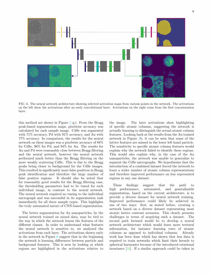
FIG. 6. The neural network architecture showing selected activation maps from various points in the network. The activationson the left show the activations after an early convolutional layer. Activations on the right come from the first concatenationlayer.

this method are shown in Figure 5 g-i. From the Braggpeak-based segmentation maps, pixelwise accuracy wascalculated for each sample image. CdSe was segmentedwith 71% accuracy, Pd with 91% accuracy, and Au with77% accuracy. In comparison, the results for the neuralnetwork on these images was a pixelwise accuracy of 88%for CdSe, 96% for Pd, and 94% for Au. The results forAu and Pd were reasonably close between Bragg filteringand the neural network, however the neural networkperformed much better than the Bragg filtering on themore weakly scattering CdSe. This is due to the Braggpeaks being closer to background for the CdSe images.This resulted in significantly more false positives in Braggpeak identification and therefore the large number offalse positive regions. It should also be noted thatfor reasonably good results for the Bragg filtering case,the thresholding parameters had to be tuned for eachindividual image, in contrast to the neural network.The neural network required no tuning to the individualmicrograph and was successful in its segmentation taskimmediately for all three sample types. This highlightsthe truly automated nature of CNN-based segmentation.

The better segmentation for Au nanoparticles, by theneural network trained on mixed data, may be tied tothe way in which the network learns the features of thedifferent classes. In order to understand what featuresthe neural network is sensitive to, we analyzed theactivations from each layer. The activations shown earlyin the network in Figure 6 suggest that in the beginningthe network is learning differences between particle andbackground features. This is seen by looking at whichregions are highlighted in the activations relative to

the image. The later activations show highlightingof specific atomic columns, suggesting the network isactually learning to distinguish the actual atomic columnfeatures. Looking back at the results from the Au trainednetwork in Figure 2b, it can be seen that some of thelattice features are missed in the lower left hand particle.The sensitivity to specific atomic column features wouldexplain why the network failed to identify these regions.This would also explain why, in the case of the Aunanoparticles, the network was unable to generalize tosegment the CdSe micrographs. We hypothesize that theintroduction of a combined dataset forced the network tolearn a wider number of atomic column representationsand therefore improved performance on less representedregions in any one dataset.

These findings suggest that the path tohigh performance, automated, and generalizablesegmentation, based on the current architecture, is toprovide a diverse dataset for neural network training.Improved performance could likely be achieved inone of two ways: first, as stated before, creating anetwork based on a diverse dataset representing mostatomic lattice contrast scenarios. This clearly presentschallenges in terms of acquiring such a dataset. Thesecond path forward would be to develop a neuralnetwork architecture which would learn more texturalinformation, for instance learning rows of atomiccolumns as opposed to individual columns. Alreadywork has been done which has shown that less data isrequired to train networks which limit their kernels tospherical harmonics because of the introduced rotationalinvariance [34]. If a similar approach could be taken in

9

order to favor learning textures, performance could alsopotentially improve.

The results presented show the potential for developingautomated characterization. We have been able totrain the U-Net architecture to segment images formaterials with variable scattering factors. Automatedsegmentation, such as this, could then be used as abase for further automated classification of local atomicstructures, including defects. Ultimately, statistics basedon these classifications of local atomic structures could beused to help enhance prediction of material structuresand the influence of local structural heterogeneity onproperties and performance.

IV. CONCLUSION

Segmentation using neural networks on HRTEMimages which include a crystalline region and amorphousbackground is a new area of exploration. Thismethod could have impact on high throughput materialscharacterization in the HRTEM. We have shownthat a U-Net architecture can achieve state-of-the-artsegmentation results on HRTEM images. Segmentationusing U-Net appears to depend strongly on learningatomic column representations. We have also determinedthat accurate location of particles is not dependent onmass thickness contrast but instead on the presence ofatomic columns, which is promising for the applicationto low atomic number materials. We have also foundthat training on a diverse set of materials leads to themost generalizable neural network, as well as overallenhanced accuracy across the test set. Additionally,the developed neural network is able to outperformtraditional segmentation techniques such as Braggpeak filtering on low atomic number materials by afairly significant margin. We have also demonstratedthe possibility of a high throughput characterizationpipeline using HRTEM. While this study was nothigh throughput, each individual part used automatedtechniques from synthesis, to imaging, and finallysegmentation. This technique demonstrates the potentialof CNNs as the base for further analysis and classificationtools for local atomic structure.

V. DATA AVAILABILITY

The complete workflow for micrograph preprocessing,network training, and testing is available in Jupyternotebooks at https://github.com/ScottLabUCB/HTTEM/tree/master/pyNanoFind

VI. ACKNOWLEDGEMENTS

Work at the Molecular Foundry was supported bythe Office of Science, Office of Basic Energy Sciences,off the U.S. Department of Energy under Contract No.DE-AC02-05CH11231. This material is based upon worksupported by the National Science Foundation GraduateResearch Fellowship under Grant No. DGE-1752814.This work was also supported by National ScienceFoundation STROBE grant DMR-1548924. CdSesynthesis was supported by the Department of Energy,Office of Energy Efficiency and Renewable Energy(EERE), under Award Number DE-EE0007628. Theauthors would like to thank Haoran Yang and EmoryChan for providing the CdSe nanoparticles. The authorswould also like to thank Colin Ophus, Mike MacNeil, andTess Smidt for their feedback and comments during thewriting of this manuscript.

VII. AUTHOR CONTRIBUTIONS

M.C.S. and C.K.G. conceived the project and designedthe experiments. C.K.G. and C.G. optimized the networkarchitecture. C.K.G. acquired the training images,trained the network, and tested the network. C.K.G.and M.C.S. wrote the manuscript. All authors discussedthe results and commented on the manuscript.

VIII. COMPETING INTERESTS

The authors declare no competing financial ornon-financial interests.

[1] Jain, A. et al. Commentary: The materials project:A materials genome approach to accelerating materialsinnovation. APL Materials 1, 011002 (2013).

[2] Needs, R. J. & Pickard, C. J. Perspective: Role ofstructure prediction in materials discovery and design.APL Materials 4, 053210 (2016).

[3] Hattrick-Simpers, J. R., Gregoire, J. M. & Kusne, A. G.Perspective: Composition–structure–property mappingin high-throughput experiments: Turning data intoknowledge. APL Materials 4, 053211 (2016).

[4] Tabor, D. P. et al. Accelerating the discovery of materialsfor clean energy in the era of smart automation. NatureReviews Materials 3, 5–20 (2018).

[5] Chan, E. M. et al. Reproducible, high-throughputsynthesis of colloidal nanocrystals for optimization inmultidimensional parameter space. Nano Letters 10,1874–1885 (2010).

[6] Zhao, S. et al. Influence of atomic-level morphologyon catalysis: The case of sphere and rod-like goldnanoclusters for CO 2 electroreduction. ACS Catalysis8, 4996–5001 (2018).

10

[7] Orfield, N. J., McBride, J. R., Keene, J. D., Davis,L. M. & Rosenthal, S. J. Correlation of atomicstructure and photoluminescence of the same quantumdot: Pinpointing surface and internal defects that inhibitphotoluminescence. ACS Nano 9, 831–839 (2015).

[8] Green, M. L. et al. Fulfilling the promise of the materialsgenome initiative with high-throughput experimentalmethodologies. Applied Physics Reviews 4, 011105(2017).

[9] Rasool, H. I., Ophus, C., Klug, W. S., Zettl, A. &Gimzewski, J. K. Measurement of the intrinsic strengthof crystalline and polycrystalline graphene. NatureCommunications 4 (2013).

[10] House, S. D., Chen, Y., Jin, R. & Yang, J. C.High-throughput, semi-automated quantitative STEMmass measurement of supported metal nanoparticlesusing a conventional TEM/STEM. Ultramicroscopy 182,145–155 (2017).

[11] Ophus, C., Shekhawat, A., Rasool, H. & Zettl,A. Large-scale experimental and theoretical study ofgraphene grain boundary structures. Physical Review B92 (2015).

[12] Laramy, C. R., Brown, K. A., O’Brien, M. N. & Mirkin,C. A. High-throughput, algorithmic determination ofnanoparticle structure from electron microscopy images.ACS Nano 9, 12488–12495 (2015).

[13] Szegedy, C., Toshev, A. & Erhan, D. Deep neuralnetworks for object detection. In Burges, C. J. C.,Bottou, L., Welling, M., Ghahramani, Z. & Weinberger,K. Q. (eds.) Advances in Neural Information ProcessingSystems 26, 2553–2561 (Curran Associates, Inc., 2013).

[14] Ronneberger, O., Fischer, P. & Brox, T. U-net:Convolutional networks for biomedical imagesegmentation. In Navab, N., Hornegger, J., Wells,W. M. & Frangi, A. F. (eds.) Medical Image Computingand Computer-Assisted Intervention – MICCAI 2015,vol. 9351, 234–241 (Springer International Publishing,2015).

[15] Nicholson, W. V. & Glaeser, R. M. Review: Automaticparticle detection in electron microscopy. Journal ofStructural Biology 133, 90–101 (2001).

[16] Wang, F. et al. DeepPicker: A deep learning approachfor fully automated particle picking in cryo-EM. Journalof Structural Biology 195, 325–336 (2016).

[17] Fultz, B. & Howe, J. Transmission ElectronMicroscopy and Diffractometry of Materials (SpringerBerlin Heidelberg, 2013).

[18] Ziatdinov, M. et al. Deep learning of atomicallyresolved scanning transmission electron microscopyimages: Chemical identification and tracking localtransformations. ACS Nano 11, 12742–12752 (2017).

[19] Madsen, J. et al. A deep learning approach to identifylocal structures in atomic-resolution transmissionelectron microscopy images. Advanced Theory andSimulations 1, 1800037 (2018).

[20] Ziatdinov, M. A., Dyck, O., Jesse, S. & Kalinin,S. V. Atomic mechanisms for the si atom dynamics ingraphene: chemical transformations at the edge and inthe bulk (2019).

[21] Maksov, A. et al. Deep learning analysis of defectand phase evolution during electron beam-inducedtransformations in WS2. npj Computational Materials5, 12 (2019).

[22] Schiøtz, J. et al. Identifying atoms in highresolution transmission electron micrographs using adeep convolutional neural net. Microscopy andMicroanalysis 24, 512–513 (2018).

[23] Schiøtz, J. et al. Using neural networks to identifyatoms in hrtem images. Microscopy and Microanalysis25, 216–217 (2019).

[24] Kalinin, S. V. et al. Lab on a beam—big data andartificial intelligence in scanning transmission electronmicroscopy. MRS Bulletin 44, 565–575 (2019).

[25] Groom, D. J. et al. Automatic segmentation of inorganicnanoparticles in BF TEM micrographs. Ultramicroscopy194, 25–34 (2018).

[26] Get started with the image labeler - MATLAB &simulink. URL https://www.mathworks.com/help/

vision/ug/get-started-with-the-image-labeler.

html.[27] Schorb, M., Haberbosch, I., Hagen, W. J. H., Schwab,

Y. & Mastronarde, D. N. Software tools for automatedtransmission electron microscopy. Nature Methods(2019).

[28] Lim, B., Xiong, Y. & Xia, Y. A water-basedsynthesis of octahedral, decahedral, and icosahedral pdnanocrystals. Angewandte Chemie International Edition46, 9279–9282 (2007).

[29] F. Niekiel, C. O. T. P., P. Ercius. openNCEM (2016–).URL https://openncem.readthedocs.io/en/latest/.

[30] Geron, Aurelien. Hands-On Machine Learning withScikit-Learn & TensorFlow (O’Reilly Media, 2017), 1edn.

[31] Chollet, F. Keras (2015–2019). URL https://keras.

io/.[32] Goodfellow, I., Bengio, Y. & Courville, A. Deep Learning

(MIT Press, 2016). http://www.deeplearningbook.org.[33] Kingma, D. P. & Ba, J. L. Adam: A Method

for Stochastic Optimization. arXiv 1–15 (2015).arXiv:1412.6980v9.

[34] Worrall, D. E., Garbin, S. J., Turmukhambetov, D. &Brostow, G. J. Harmonic networks: Deep translation androtation equivariance. CoRR abs/1612.04642 (2016).1612.04642.