Methodological issues in observational studies of ... issues in observational studies of comparative...
87
Methodological issues in observational studies of comparative effectiveness Choice of comparators, target population, and hypothesis formulation Robert J Glynn Divisions of Pharmacoepidemiology & Pharmacoeconomics Brigham & Women’s Hospital, Boston, MA
-
Upload
truonghanh -
Category
Documents
-
view
216 -
download
2
Transcript of Methodological issues in observational studies of ... issues in observational studies of comparative...

Methodological issues in observational studies of comparative effectiveness
Choice of comparators, target population, and
hypothesis formulation
Robert J Glynn
Divisions of Pharmacoepidemiology & Pharmacoeconomics Brigham & Women’s Hospital, Boston, MA

Methodological issues in observational studies of comparative effectiveness
Future talks
March: Martin Kulldorff
Sequential analysis applied to comparative effectiveness
April: Joshua Gagne Comparative effectiveness of newly marketed drugs
May: Jessica Myers
Integrating effectiveness information across outcomes

Disclosure Supported by grant AG018833 from the US National Institute on Aging
I have worked on grants from AstraZeneca and Novartis to the Brigham & Women’s Hospital for the design, monitoring and analysis of clinical trials; and signed a consulting agreement with Merck to give a grand rounds talk

Outline
1. Challenges to active comparators
2. Personal experience with non-user referents 3. Likely differential surveillance in non-users 5. Healthy starter/sick stopper bias 6. Time scale in safety/effectiveness studies 7. Propensity score trimming and focusing the target population 8. Composite endpoints and competing risks

Comparative Effectiveness Research (CER): Definition and Aims
The generation and synthesis of evidence that compares the benefits and harms of alternative methods to prevent, diagnose, treat, and monitor a clinical condition or to improve the delivery of care.*
Aim: to improve decisions that affect medical care at the levels of both policy and the individual.†
*Institute of Medicine (2009) Initial National Priorities for Comparative Effectiveness Research. †HC Sox, SN Goodman. Annu Rev Pub Health 2012

CER: Key elements (a) Head-to-head comparisons of active treatments
(b) Study populations typical of day-to-day clinical practice
(c) Focus on evidence to inform care tailored to the characteristics of individual patients*
*HC Sox, SN Goodman. Annu Rev Pub Health 2012

Example: oral diabetes drugs and cancer risk Diabetes is associated with increased risk of several common cancers*
Association may be partly due to shared risk factors such as aging, obesity, diet, and physical inactivity*
Evidence on relationships of specific antidiabetic drugs with cancer risk is limited, and possibly confounded
Early evidence suggests that metformin is associated with reduce drisk of cancer
*E Giovannucci et al. Diabetes and cancer: a consensus statement. Diabetes Care 2010

Important time scales Age in years:
risk factor for DM and cancer often the best scale for risk set construction (EL Korn et al. Am J Epidemiol 1997)
Time since DM Dx:
related to cancer risk and surveillance likely measured with differential error
Time since Rx initiation:
natural scale for Rx evaluation problematic for switchers and those with gaps

Errors in assessing duration of DM Onset date is left-censored for subjects who enter the database with DM
DM is often undiagnosed (about 27% of cases currently; formerly 50% in the US)
DM is often not recorded among discharge diagnoses, and is less often recorded in those near death
Drug treatment for DM is less frequent in frail people
RJ Glynn et al. Aging, comorbidity, and reduced rates of drug treatment for diabetes mellitus. J Clin Epidemiol 1999

Selective recording and treatment of DM
RJ Glynn et al. Agreement between drug treatment data and a discharge diagnosis of diabetes mellitus in the elderly. Am J Epidemiol 1999

Time since Rx initiation Often most relevant in pharmacoepidemiology; mimics time after randomization in a trial
Risk sets make comparisons (with active comparators) at equivalent treatment durations
Cumulative dose consumed can vary for given time because of gaps and differences in daily dose
Variant scale restricts to those with at least one (or two) refills and starts follow-up at that time
For second line therapy, duration of prior drug treatment an important covariate

Time-related biases in studies of DM and cancer Attention to time scales can prevent time-related biases, which may have distorted treatment effects in several studies finding a protective effect of metformin*
Immortal time bias: introduced with time-fixed cohort analyses that misclassify unexposed time as exposed
Time-window bias: differential exposure opportunity time windows between subjects
Time-lag bias: can occur in comparisons of treatments given at different stages of disease
S Suissa, L Azoulay.. Metformin and the risk of cancer: time-related biases in observational studies. Diab Care 2012

Alternative comparison groups/time scales Non-diabetic individuals followed from a specific time point
Non-diabetic initiators of another drug
Untreated diabetics
Diabetic individuals followed from initiation of a comparison drug

Limitations of non-diabetic comparators DM is an independent risk factor for cancer
Unmeasured lifestyle confounders (diet, exercise, SES, BMI) are unbalanced
Unmeasured biomarker confounders (fasting glucose, glycated hemoglobin)*
Likely differential surveillance, barriers to diagnosis/ treatment
*Emerging risk factors collaboration. Diabetes mellitus, fasting glucose, and risk of cause-specific death. NEJM 2011
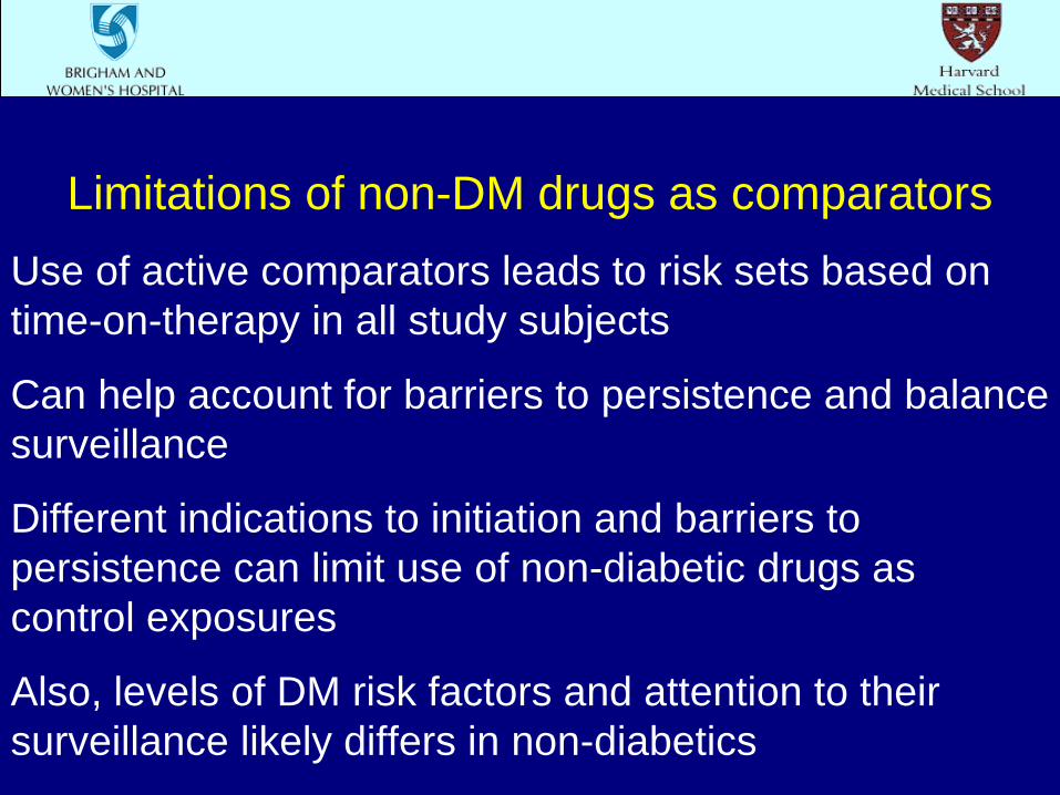
Limitations of non-DM drugs as comparators Use of active comparators leads to risk sets based on time-on-therapy in all study subjects
Can help account for barriers to persistence and balance surveillance
Different indications to initiation and barriers to persistence can limit use of non-diabetic drugs as control exposures
Also, levels of DM risk factors and attention to their surveillance likely differs in non-diabetics

Limitations of diabetic non-user comparators Diet-controlled diabetes typically less severe
Non-user referents lack treatment initiation and termination dates
Can have decreased surveillance for comorbidities relative to medication users
Often missing data on barriers to initiation and persistence
Problematic to control for duration of treatment

Distinguish placebo controls and non-user referents
Placebo controls are often natural, appropriate referents for evaluation of safety and efficacy in randomized trials
Non-user referents in observational studies differ in important ways:
Not clearly eligible or willing to initiate therapy
No clear date of initiation
No comparable assessment of treatment duration

Challenges to active comparators Other DM drugs may influence cancer risk; e.g. possible protective effects of metformin
Or be initiated after different durations of DM, according to guidelines*
Or in patients that differ on unmeasured cancer risk factors (e.g. BMI)
*DM Nathan et al. Medical management of hyperglycemia in type 2 diabetes: a consensus algorithm for the initiation and adjustment of therapy. Diabetes Care 2009

Advantages of DM drugs as comparators In spite of guidelines, uncertainty about treatments leads to substantial variability in actual practice
Comparisons among active, within-class drugs address comparative safety & efficacy questions
Comparisons restricted to treated patients with diabetes offer a better chance for confounder control, especially in claims data

Three paradoxes with non-user referents
1. Among hospitalized, older people enrolled in state-sponsored drug benefits programs, diabetes diagnosis and treatment were associated with enhanced survival vs no dx or rx
2. Across 20 commonly used classes of drugs, users vs non-users of several classes had markedly reduced death rates, of a magnitude inconsistent with randomized evidence
3. Focused analysis (e.g. propensity score matching) did little to
reduce the magnitude of the incredible reduction in the hazard of death in users vs non-users of lipid-lowering drugs

Observational data on mortality with non-user referent
Glynn et al. Paradoxical relations of drug treatment with mortality in older persons. Epidemiology 2001

Observational data on mortality with non-user referent
Glynn et al. Selective prescribing led to overestimation of the benefits of lipid lowering drugs. J Clin Epidemiol 2006

Variable surveillance in effectiveness/safety studies: exposure assessment
Initiation of treatments is generally measured well in administrative databases (although whether subjects actually take medications is unknown)
Duration of exposure indexed by prescription refills
Assessment of exposure duration is problematic with coverage gaps (e.g. nursing home stays)
Non-user referents lack initiation dates or comparable assessment of duration of exposure

Variable surveillance in effectiveness/safety studies: outcome assessment
Exposed subjects are often followed more intensively
Especially intensive for anticipated outcomes such that these may not be evaluable in observational designs*
Even for unanticipated effects, prescribers may follow treated patients more intensively than non-user referents
Randomized trials often block on center as a way to balance outcome surveillance
JP Vandenbroucke. When are observational studies as credible as randomized trials? Lancet 2004; 363: 1728-31.

Variable surveillance in effectiveness/safety studies: covariate assessment
Treatment initiators generally have more intensive surveillance than non-initiators
Database studies usually assume comorbid conditions are absent unless expressly noted
Comorbidities related to treatment decisions may be particularly scrutinized
Little prior study of whether covariate scrutiny is jointly related to treatment and disease risk

Design strategies to balance surveillance in effectiveness/safety studies
Often studies restrict populations to subjects with demonstrated eligibility and those who meet some system use criteria (e.g. history of filled prescriptions through the system)
Can also reduce surveillance variability by restriction to subjects with documented risk levels for the outcome; e.g. prior MI or diagnosed ESRD
Even with such restrictions, treatment initiators will likely have greater surveillance than non-initiators

Differential covariate assessment in non-users
J Hippisley-Cox & C Coupland. BMJ 2010

Differential covariate assessment in non-users
J Hippisley-Cox & C Coupland. BMJ 2010

Does comparability of information between exposed and unexposed matter?
Not necessarily!
Comparability-of-information principle dictates the importance of equivalent information in compared groups*
Rothman & Greenland† argue against the principle
Nondifferential measurement error does not guarantee that bias is toward the null
e.g. a case-control study using proxy respondents for cases might have greater bias with proxy responses for controls
*S Wacholder et al. Selection of controls in case-control studies I: principles. Am J Epidemiol 1992; 135: 1019-1028. †K Rothman, S Greenland. Modern Epidemiology 2nd ed. Lippincott-Raven 1998.

Does confounder measurement error matter? Investigators often focus on accurate exposure and outcome assessment, with a more sanguine view of errors in confounders*
Non-differential confounder misclassification biases toward the crude, can induce artificial heterogeneity of effects across confounder categories, but is somewhat limited in magnitude†
Differential confounder misclassification can bias in either direction and yield much greater heterogeneity in estimates across confounder categories.
Sensitivity analyses are needed to evaluate potential impact of inaccurate confounder assessment
*AM Walker & SF Lanes. Misclassification of covariates. Stat Med 1991; 10: 1181-96. †H Brenner. Bias due to non-differential misclassification of polytomous confounders. J Clin Epidemiol 1993; 46: 57-63.
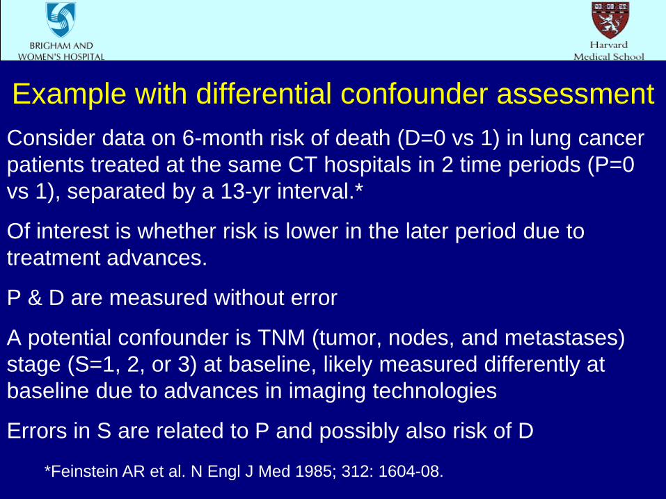
Example with differential confounder assessment Consider data on 6-month risk of death (D=0 vs 1) in lung cancer patients treated at the same CT hospitals in 2 time periods (P=0 vs 1), separated by a 13-yr interval.*
Of interest is whether risk is lower in the later period due to treatment advances.
P & D are measured without error
A potential confounder is TNM (tumor, nodes, and metastases) stage (S=1, 2, or 3) at baseline, likely measured differently at baseline due to advances in imaging technologies
Errors in S are related to P and possibly also risk of D *Feinstein AR et al. N Engl J Med 1985; 312: 1604-08.

Impact of confounder measurement error Hypothetical study
Consider a prospective study of statin use (S=0 vs 1) and occurrence of venous thromboembolism (VTE=0 or 1)
Obesity (O=0 or 1) is strongly related to statin use and VTE risk
Available is a surrogate of O, O*, measured with sensitivity (Pr(O*=1|O=1)) Se, and specificity (Pr(O*=1|O=0)) Sp
Se and Sp might be non-differential, or differential, i.e. dependent on S, VTE, or both

Impact of confounder measurement error Hypothetical true data
O=0 VTE=1 VTE=0 Total Risk S=1 10 490 500 .02 S=0 190 9310 9500 .02
O=1 VTE=1 VTE=0 Total Risk
S=1 60 940 1000 .06
S=0 240 3760 4000 .06 OR0=1.00 OR1=1.00 ORcrude=1.49 ORadj=1.00

Impact of confounder measurement error Non-differential error: O* has Se=.7; Sp=.8
O*=0 VTE=1 VTE=0 Total Risk S=1 26 674 700 .037 S=0 224 8576 8800 .025
O*=1 VTE=1 VTE=0 Total Risk
S=1 44 756 800 .055
S=0 206 4494 4700 .044 OR0=1.48 OR1=1.27 ORcrude=1.49 ORadj=1.34

Differential confounder measurement error S=0: O* Se=.6, Sp=.7; Se=1: O* Se=.8, Sp=.9
O*=0 VTE=1 VTE=0 Total Risk S=1 21 629 650 .032 S=0 229 8021 8250 .028
O*=1 VTE=1 VTE=0 Total Risk
S=1 49 801 850 .058
S=0 201 5049 5250 .038 OR0=1.17 OR1=1.54 ORcrude=1.49 ORadj=1.40

Differential error in sensitivity only S=0: O* Se=.5; S=1: O* Se=.8
O*=0 VTE=1 VTE=0 Total Risk S=1 22 678 700 .031 S=0 310 11190 11500 .027
O*=1 VTE=1 VTE=0 Total Risk
S=1 48 752 800 .06
S=0 120 1880 2000 .06 OR0=1.17 OR1=1.00 ORcrude=1.49 ORadj=1.06
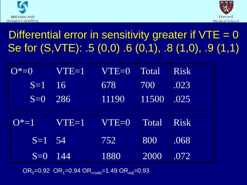
Differential error in sensitivity greater if VTE = 0 Se for (S,VTE): .5 (0,0) .6 (0,1), .8 (1,0), .9 (1,1)
O*=0 VTE=1 VTE=0 Total Risk S=1 16 678 700 .023 S=0 286 11190 11500 .025
O*=1 VTE=1 VTE=0 Total Risk
S=1 54 752 800 .068
S=0 144 1880 2000 .072 OR0=0.92 OR1=0.94 ORcrude=1.49 ORadj=0.93

Time period (P), and death (D) by stage (S) StageA 1 2 3 D=1 D=0 D=1 D=0 D=1 D=0 P=1 2 22 5 13 52 37 P=0 70 211 74 98 571 242 RR .33 .65 .83 StageB 1 2 3
D=1 D=0 D=1 D=0 D=1 D=0 P=1 10 32 8 17 41 23 P=0 70 211 74 98 571 242 RR .96 .74 .91
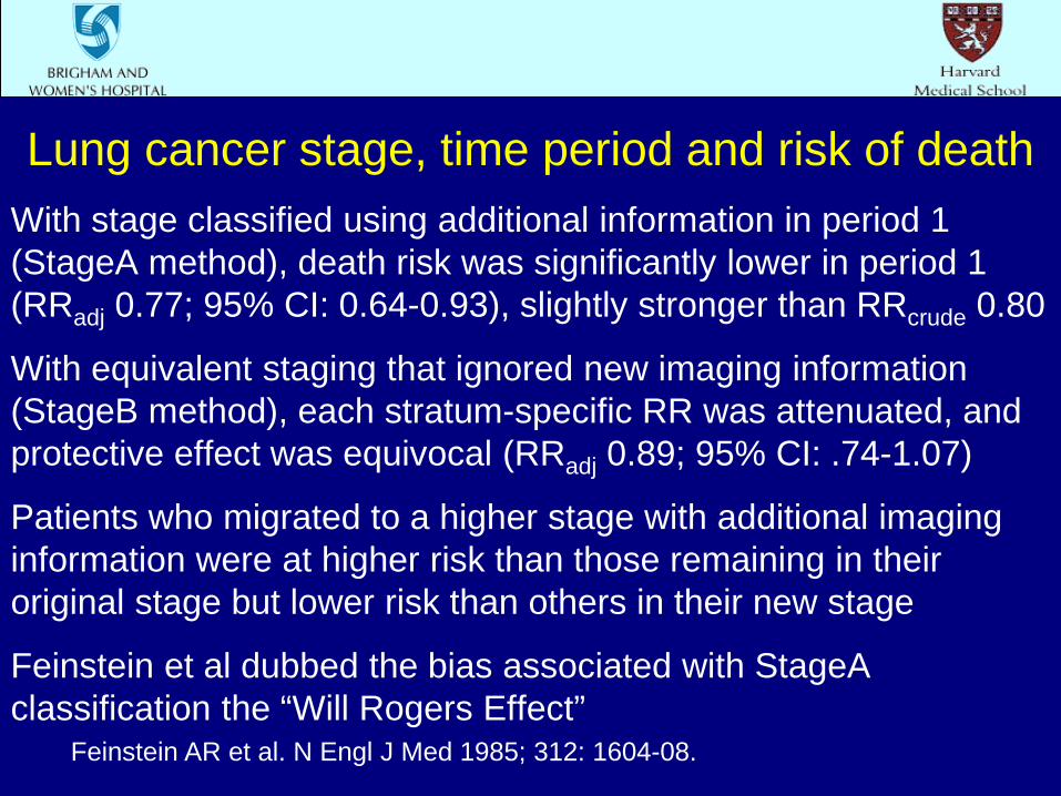
Lung cancer stage, time period and risk of death With stage classified using additional information in period 1 (StageA method), death risk was significantly lower in period 1 (RRadj 0.77; 95% CI: 0.64-0.93), slightly stronger than RRcrude 0.80
With equivalent staging that ignored new imaging information (StageB method), each stratum-specific RR was attenuated, and protective effect was equivocal (RRadj 0.89; 95% CI: .74-1.07)
Patients who migrated to a higher stage with additional imaging information were at higher risk than those remaining in their original stage but lower risk than others in their new stage
Feinstein et al dubbed the bias associated with StageA classification the “Will Rogers Effect”
Feinstein AR et al. N Engl J Med 1985; 312: 1604-08.

Parallels between the healthy worker effect and biases in studies of preventive drug use
1. Healthy hire effect similar to selection of healthier individuals for preventive drug therapy: healthy starter effect
2. Healthy worker survivor effect similar to better adherence in healthier people: sick stopper effect
3. Inevitable aging effect applies in both situations
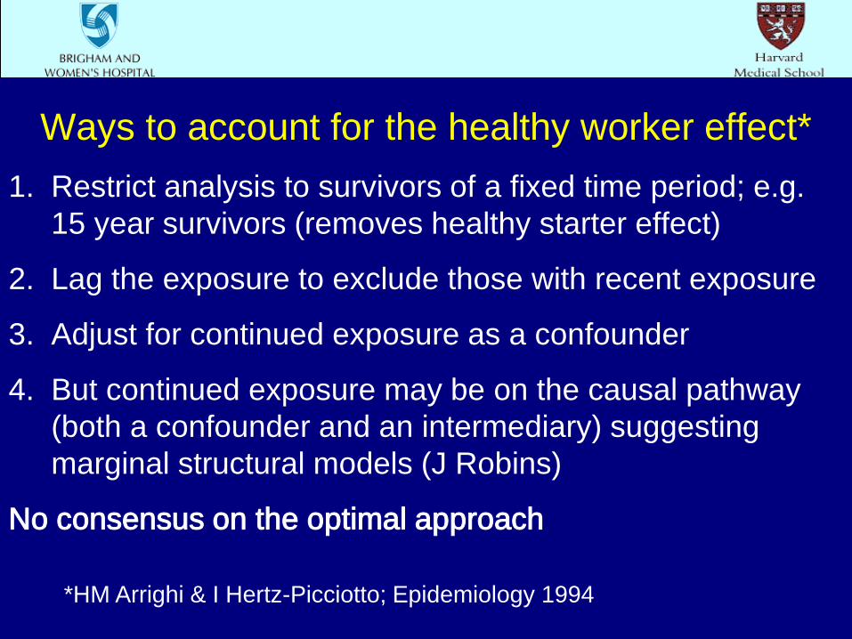
Ways to account for the healthy worker effect* 1. Restrict analysis to survivors of a fixed time period; e.g.
15 year survivors (removes healthy starter effect)
2. Lag the exposure to exclude those with recent exposure
3. Adjust for continued exposure as a confounder
4. But continued exposure may be on the causal pathway (both a confounder and an intermediary) suggesting marginal structural models (J Robins)
No consensus on the optimal approach
*HM Arrighi & I Hertz-Picciotto; Epidemiology 1994

The time scale for occupational and pharmacoepidemiologic studies
1. Time since hire relates to outcomes in two ways: the healthier workers stay longer in the workforce; yet their health inexorably declines with age
2. It is critical to control for time since hire*
3. Parallel considerations argue for the need to control for time since initiation and time on therapy in pharmacoepidemiology
*WD Flander et al. Epidemiology 1993

Selective use of preventive therapies Complex factors influence use of preventive therapies
Healthy user bias arises from unmeasured determinants of use
Bias can be large and changed little by control for available covariates
Intractable to standard analytic strategies, not just in claims databases

The Healthy Starter Effect Complex factors influence decisions to initiate preventive therapies
Providers may focus on a patient’s main or most symptomatic medical problem (DA Redelmeier et al N Engl J Med 1998)
Preventive strategies may be less beneficial with short life expectancy
Measurement and control for frailty is very difficult, so substantial confounding may remain with traditional approaches

The Sick Stopper Effect Just as starting a preventive regimen is a sign of good health, sticking with a therapy is a sign of healthy behaviors and good health
Determinants of stopping may differ from and be more difficult to measure than those for starting
Stoppers are probably a mixed population, including those near death and those who lose ascertainable medication use through institutionalization
Their exclusion may represent depletion of susceptibles

Value of new user designs* Many studies of drug effects have included prevalent users
This increases sample size, but precludes evaluation of time on study
Effects of a drug may vary by duration of use, e.g. for hormone therapy or coxibs
RCTs control precisely for time on therapy
*WA Ray. Am J Epidemiol 2003; 158: 915-920

More value in studying new users Confounders affecting initiation may differ from those affecting persistence
With prevalent users, need to consider propensity to start and propensity to persist: these may differ
Stoppers of preventive drugs are often sick
Risk factors may be affected by use of study drugs, e.g. NSAIDS influence BP, and HT influences CRP
May not be possible to control for these factors on the causal pathway if measured long after initiation

Limitations of new user designs Reduced power and generalizability through exclusion of long-term users
But long-term users are selected survivors with missing indications for drug initiation
Real-time assessment of determinants of drug initiation may be expensive
But available in computerized databases of medical encounters

Example: non-user vs active referents in a study of NSAIDS & CVD*
Prospective cohort study of CV risks of new use of NSAIDS
Beneficiaries age 65+ in Pennsylvania’s PACE program and in Medicare
Exposed subjects had no NSAID Rx for 6 months before a new Rx
Referent groups: non-users vs new users of glaucoma drugs or thyroid hormones *DH Solomon et al. Arth Rheum 2006; 54:1378-89

Adjusted rate ratios of CVD* New user referent Never user referent
Drug RR CI RR CI
Diclofenac 1.10 0.89-1.37 1.62 1.18-2.22
Ibuprofen 0.96 0.81-1.14 1.25 0.97-1.59
Naproxen 0.75 0.62-0.92 1.04 0.79-1.37
*From a proportional hazards model; outcome is new MI or stroke

Design approaches for healthy users
S Schneeweiss et al Med Care 2007

Impact of restriction on hazard ratios

Limitations of never user referents Non-users may have different utilization of prescription programs and physicians
Surveillance of their health may be less complete
Covariates may be measured with different errors than regular users of programs
Such confounding may not be controllable

Summary In a new user study, choice of an appropriate active referent group can be challenging
The comparison treatment will have its own efficacy and safety profile which can complicate interpretation
However, individuals initiating that alternative will be active within the system, willing to start a new therapy, and screened for its appropriateness
In many circumstances, inferences from such a comparison will be more valid than those obtained from a passive, non-user referent group

Summary confounder scores in study design Randomized trials use eligibility (exclusion) criteria to target patients most likely to benefit and limit side effects
Often leads to exclusion of older, sicker patients, leaving clinicians uncertain about effectiveness in these patients
e.g. seminal trial of oxaliplatin for colon cancer (T Andre et al; NEJM 2004) excluded patients >75 years old, yet the disease occurs frequently in this group
CER can use disease risk scores and propensity scores to target populations at reasonable risk and with treatment uncertainty in whom valid comparisons are possible

Value of summary confounder scores* Reduce the frequently high dimension of confounding variables
Both propensity scores and disease risk scores have inherent scientific interest in studies of drug use and outcomes
Both scores provide a natural scale for evaluation of effect modification
Both provide a ready way to identify areas of non-overlap between treatment groups
*OS Miettinen. Am J Epidemiol 1976

Value of summary confounder scores* While propensity scores (and perhaps also disease risk scores) are often seen as analysis tools, they can (and should) play a role in study design
Propensity score matching (as well as stratification and weighting approaches) focus on similar subjects who might receive either treatment
Propensity score development and subject selection can occur before consideration of outcome data
*DB Rubin. The design versus the analysis of observational studies for causal effects: parallels with the design of randomized trials. Stat Med 2007

Examples of disease risk scores Framingham risk score for prediction of a first major coronary event
Gail model for prediction of incident breast cancer
APACHE II score for ICU survival
Charlson comorbidity index predicting mortality from administrative data

Challenges to propensity score estimation Sometimes we do not have large numbers of exposed and unexposed subjects for propensity score estimation
E.g. when studying newly marketed drugs; or unusual (e.g. high) doses; or multi-category exposures
Propensity scores may evolve with time, especially after introduction of a new therapy
Strong predictors of exposure without effect on the outcome should be excluded (MA Brookhart et al; AJE 2006), and these are difficult to identify in the above situations
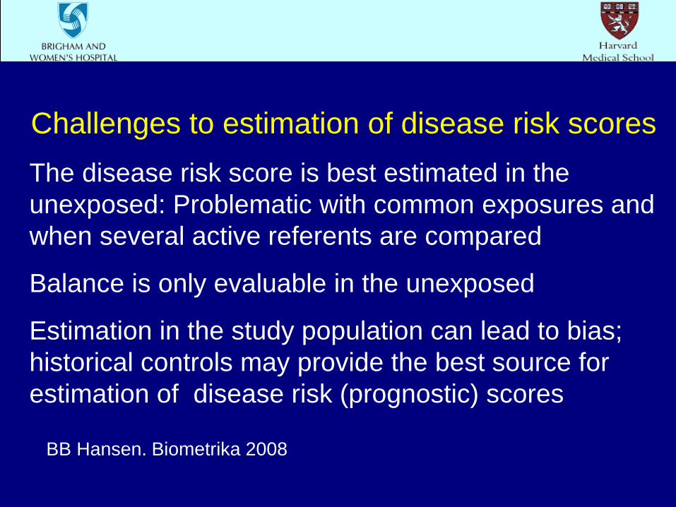
Challenges to estimation of disease risk scores The disease risk score is best estimated in the unexposed: Problematic with common exposures and when several active referents are compared
Balance is only evaluable in the unexposed
Estimation in the study population can lead to bias; historical controls may provide the best source for estimation of disease risk (prognostic) scores
BB Hansen. Biometrika 2008

Joint matching on the propensity score (PS) and disease risk score (DRS)
Straightforward to minimize the distance between (PS, DRS) pair in exposed and unexposed subjects
With two (or more) exposed groups (versus standard treatment), can minimize distance in three dimensions (PS1, PS2, DRS)
With common exposures and less data on outcomes, emphasize (overweight) distance on the PS dimension
With new or rare treatments, emphasize DRS dimension

Settings favoring disease risk scores Initiatives such as the FDA’s sentinel system seek to identify adverse effects and benefits of drugs and new doses as soon after marketing as possible
In the short-term after marketing, propensity scores may be unreliable or evolving
Historical data on outcomes in people treated before use of the new drug or dose can characterize risk

Example: new statins & doses after heart attack* The randomized 4S (1994), CARE (1996) and LIPID (1998) trials proved the value of statin therapy after myocardial infarction (MI) for prevention of recurrent MI, stroke and death
Later trials (PROVE-IT TIMI 22 [2004]; TNT [2005]) showed that higher statin doses (with atorvastatin) yielded greater benefits
We considered disease risk scores to account for confounding in observational data on atorvastatin & statin dose post-MI from 1995-2004 *RJ Glynn et al. Pharmacoepidemiology and Drug Safety 2012

Data: statins post MI We studied the 5,668 enrollees, aged 65-100 years, in either New Jersey or Pennsylvania’s state-sponsored pharmacy assistance program (PAAD or PACE) who survived an MI and filled a statin prescription within 30 days after discharge from 1995-2004
Exposures of interest are atorvastatin (available starting in 1997) and high-dose statins* (almost never used until 1997)
Outcome was recurrent MI, stroke or death within 1 yr
*NK Choudhry et al. Heart 2007


Estimate a disease risk scores Use data from low-dose, non-atorvastatin users to develop a disease risk score in the period 1995-1997
Among 826 statin initiators post MI, 203 had recurrent MI, stroke or died within 1 year
Consider demographic variables, comorbidities, and system use as predictors of outcome
Logistic model has C-statistic 0.704

Predictors of MI/Stroke/Death in 1 yr Variable Odds ratio 95% CI
Age (1 yr) 1.05 1.02-1.08
Male 1.2 0.8-1.7
Black race 2.9 1.5-5.6
Other race 1.1 0.2-5.7
NJ vs PA 1.2 0.8-1.7
MI hosp. 5-6 days 1.2 0.7-2.1
MI hosp. 7-9 days 1.4 0.8-2.5
MI hosp. 10+ days 1.5 0.8-2.6

Predictors of MI/Stroke/Death in 1 yr Angioplasty 0.6 0.4-0.8 Cong. heart failure 1.7 1.2-2.5 Hx stroke 0.8 0.6-1.2 Diabetes 0.8 0.5-1.2 Hypertension 0.7 0.5-1.0 Prior MI 0.9 0.5-1.7 Peripheral vasc. dis. 1.3 0.9-2.0 Chronic kidney dis. 1.1 0.7-1.7 Prior hosp. days 1.01 0.99-1.03 Charlson score (per pt) 1.2 1.1-1.4


Patient characteristics: 1997-2004 Characteristic Atorva. (n=1851) Other statin (n=3318) Age, mean
sd 78.2
6.6 78.7
6.5 Male, % 24.3 26.4 Black race, % 5.6 5.8 Angioplasty, % 62.9 61.2 Hyperten., % 80.5 81.0 CHF, % 59.9 59.9 Charlson score 2.6
2.0 2.5
2.0
Disease risk 26.4
15.2 27.0
15.7

Patient characteristics: 1997-2004 Characteristic Hi dose (n=922) Standard dose (n=4247) Age, mean
sd 77.7
6.5 78.7
6.5 Male, % 24.8 25.8 Black race, % 6.5 5.5 Angioplasty, % 63.9 61.3 Hyperten., % 83.1 80.3 CHF, % 61.4 59.5 Charlson score 2.7
2.1 2.5
2.0
Disease risk 26.2
15.3 26.9
15.6

Atorvastatin, dose & outcomes: 1997-2004 After 1996, 5169 post-MI patients initiated statin therapy, 1163 (22.5%) of whom had another MI, stroke, or died within 1 year
Those without an event had median predicted risk of 0.217 (IQR: 0.137-0.328)
Those with an event had median predicted risk of 0.308 (IQR: 0.197-0.434)
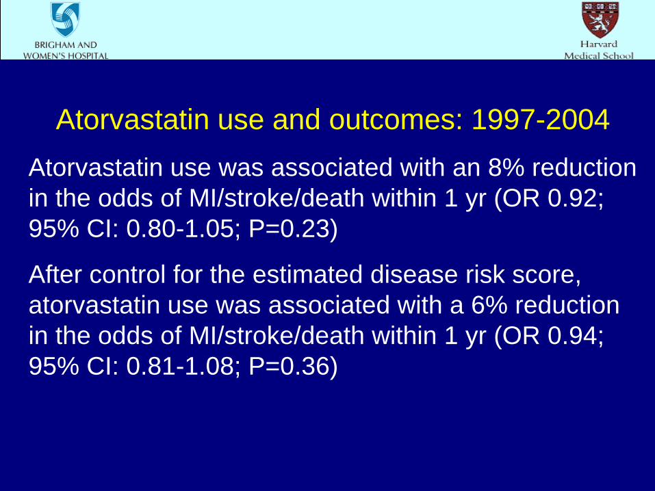
Atorvastatin use and outcomes: 1997-2004 Atorvastatin use was associated with an 8% reduction in the odds of MI/stroke/death within 1 yr (OR 0.92; 95% CI: 0.80-1.05; P=0.23)
After control for the estimated disease risk score, atorvastatin use was associated with a 6% reduction in the odds of MI/stroke/death within 1 yr (OR 0.94; 95% CI: 0.81-1.08; P=0.36)

High dose statin and outcomes: 1997-2004 Use of a high dose statin was associated with a 7% reduction in the odds of MI/stroke/death within 1 yr (OR 0.93; 95% CI: 0.78-1.11; P=0.41)
After control for the estimated disease risk score, high-dose statin use was associated with a 5% reduction in the odds of MI/stroke/death within 1 yr (OR 0.94; 95% CI: 0.80-1.13; P=0.56)

Possible effect modification by DRS quintiles DRS Observed risk % (events/exp.) Quintile Atorvastatin Other statin OR (95% CI) 1 12.6 (48/381) 10.4 (68/652) 1.21 (0.9-1.7) 2 15.7 (59/375) 17.8 (117/659) 0.89 (0.7-1.2) 3 19.2 (71/369) 21.8 (145/665) 0.88 (0.7-1.1) 4 29.5 (108/366) 27.5 (184/668) 1.07 (0.9-1.3) 5 31.4 (113/360) 37.1 (250/674) 0.85 (0.7-1.0)

Propensity score limitations Fitting a propensity score in early follow-up was problematic:
During 1997-98, only 68 subjects used high-dose statins
Propensity score fitted in this period with the 20 covariates of interest showed evidence of over-fitting
Coefficients in this PS had large differences from estimates in a model fitted to data from 1999-2004
Unclear whether differences represented sampling variability or true changes in treatment preferences

Treatment effect heterogeneity across PS strata Apparently different treatment effects in the tails of the PS can substantially influence estimated treatment effects, possibly due to unmeasured confounding
Example: T Kurth et al (AJE 2006) found raised death rates only in the subgroup of stroke patients who received TPA (vs untreated) with a low PS for treatment
Also, M Lunt et al (AJE 2010) found raised death rates in rheumatoid arthritis patients who received biologics (vs untreated) with a low PS, but a protective effect among those with a high PS

Trimming to the population with equipoise
Propensity scores can also aid in the identification of the individuals with reasonable probability of receiving either treatment of interest Trimming of subjects in both tails of the propensity score can reduce bias under a range of reasonable scenarios Treatment effect estimates based on such range restrictions do not correspond to a causal parameter, but may be less prone to bias from unmeasured confounding
T Stürmer et al, Am J Epidemiol 2009

Trimming to the population with equipoise

Design issues in 3-way CE studies
Comparison of safety and effectiveness of 3 alternative treatments involves special considerations For example, DH Solomon et al (Arch Intern Med 2010) compared 3 analgesics (nonselective NSAIDS, coxibs, and opioids) in arthritis patients in a new-user design Solomon et al created two 1-1 matches with an nsNSAID patient matched to an opioid initiator and separately to a coxib initiator, based on 2 PSs with nsNSAIDs as the referent

Design issues in 3-way CE studies
The design of Solomon et al evaluates patients with comparable propensities to all three analgesics An alternative approach uses a single generalized propensity score based on multinomial logistic regression, and forms 1:1:1 matches for comparison (JA Rassen et al. Epidemiology 2013). Simulations suggest that this alternative may reduce bias. Separate comparisons of each of the 3 pairs of treatments would include more subjects but would not identify the best treatment for a patient who could reasonably get any of the 3 treatments

Hypothesis formulation in CE studies Should design of CE studies proceed from the perspective of a superiority or an equivalence trial?
With approved drugs, perhaps the assumption of equivalence is reasonable
Noninferiority trials often require large sizes
CE studies can consider multiple endpoints; e.g. Solomon et al (Arch Intern Med 2010) considered 14 individual and 6 composite endpoints in 3 analgesic treatment groups

Hypothesis formulation in equivalence trials Exact equivalence (the null hypothesis) cannot be proven
Specify δ such that smaller differences are clinically inconsequential
Here H0: differences are less than δ; vs Ha: differences are at least δ
Under H0, the upper 100(1-α)% CI will not exceed δ with probability 1-β
Need β small to ensure a new therapy is allowed to replace an older standard (LM Friedman et al. Fundamentals of Clinical Trials; 3rd edition)
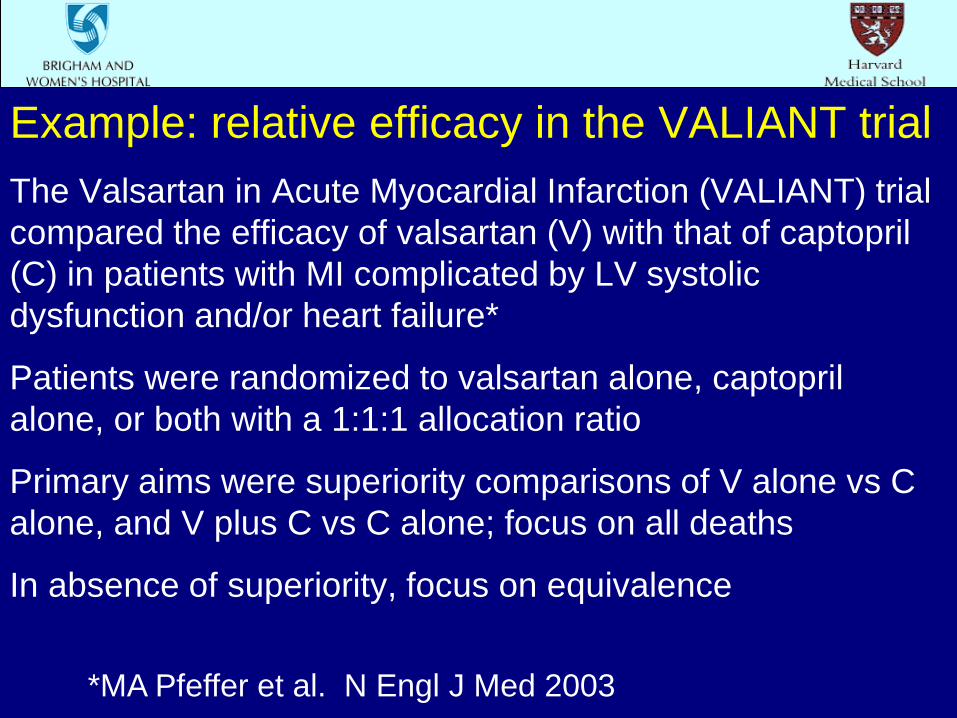
Example: relative efficacy in the VALIANT trial The Valsartan in Acute Myocardial Infarction (VALIANT) trial compared the efficacy of valsartan (V) with that of captopril (C) in patients with MI complicated by LV systolic dysfunction and/or heart failure*
Patients were randomized to valsartan alone, captopril alone, or both with a 1:1:1 allocation ratio
Primary aims were superiority comparisons of V alone vs C alone, and V plus C vs C alone; focus on all deaths
In absence of superiority, focus on equivalence
*MA Pfeffer et al. N Engl J Med 2003

Example: setting δ in the VALIANT trial VALIANT randomized 14,703 patients to accrue 2,700 deaths so as to have 86% power to detect a 15% reduction in risk, separately for the V vs C and V+C vs C comparisons*
Noninferiority evaluation done conditional on a null result for superiority of V vs C
Choose δ from a meta-analysis of post-MI ACE trials (SAVE, TRACE, AIRE); pooled OR for death: 0.74
Upper bound of 1.13 for V vs C HR preserves 55% of ACE survival benefit; trial had 74-88% power to find V as effective as C
*MA Pfeffer et al. N Engl J Med 2003

Alternative hypothesis formulation With n treatments compared, each with success (or adverse effect rate) Ri, i=1,…,n
Let Rmax = max(R1,…,Rn) and Rmin = min(R1,…,Rn)
Would a more relevant study goal, achievable with fewer subjects, be to identify the most or least effective treatment with high probability?
e.g. Pr(Ri=Rmax)>0.975 or Pr(Ri=Rmin)>0.975?
Adapted from: WJ Meurer et al. An overview of the Adaptive Designs Accelerating Promising Trials Into Treatments (ADAPT-IT) Project. Ann Emerg Med 2012