Method 8265: Volatile Organic Compounds in Water, Soil ...
64
Draft Revision 0 March 2002 8265 - 1 METHOD 8265 VOLATILE ORGANIC COMPOUNDS IN WATER, SOIL, SOIL GAS, AND AIR BY DIRECT SAMPLING ION TRAP MASS SPECTROMETRY (DSITMS) 1.0 SCOPE AND APPLICATION 1.1 This method uses direct sampling ion trap mass spectrometry (DSITMS) for the rapid quantitative measurement, continuous real-time monitoring, and qualitative and quantitative preliminary screening of volatile organic compounds (VOCs) in water, soil, soil gas, and air. DSITMS introduces sample materials directly into an ion trap mass spectrometer by means of a simple interface (such as a capillary restrictor). There is little if any sample preparation and no chromatographic separation. The response of the instrument to analytes in a sample is nearly instantaneous. In addition, the instrument is field transportable, rugged, and relatively easy to operate and maintain. 1.2 This method is applicable to the determination of VOCs in discrete samples taken to the laboratory and to on-site measurement and monitoring. It is best suited for semiquantitative screening, for repetitive quantitative analysis of previously characterized samples for pre-selected analytes, and for establishing the absence/presence of VOCs at the limit of detection of the operating conditions employed. Specialty applications include on-line deployment with direct-push technologies, in situ sampling, and continuous real-time monitoring of VOCs. 1.3 The method is not suited to identifying or quantitating a large number of constituents in highly complex mixtures nor to quantitating constituents at the isomeric level. Identifying unknown or unusual constituents in complex multi-component mixtures is better achieved using standard gas chromatography/mass spectrometry methods. This procedure is usually not applicable if results are required for individual positional isomers (e.g.; o-, m-, or p-xylenes) or individual geometric isomers (e.g., cis- or trans-1,2-dichloroethenes) unless unique operating conditions are developed and demonstrated. The principal limitation of the method is the need to demonstrate the absence of interfering analytes at the levels of concern before quantitative analysis can be performed. 1.4 This method is especially useful for the analysis of large numbers of samples, for screening samples, for on-site analyses, and for applications benefitting from its special sampling probes. Examples include surveys with high spatial and/or temporal resolution, plume mapping where results determine the next sampling point, monitoring a remedial action, in situ sampling of VOCs, and depth-profiling a groundwater well. 1.5 VOCs in air can be monitored continuously in real-time (~1 mass spectrum/second) at concentrations down to 50 ppbv, or lower, depending on the analyte. The method is applicable to ambient air, soil gas, headspace, process streams, and stack emissions, as well as to VOCs continuously purged from groundwater, surface water, and aqueous process streams. 1.6 This method is applicable to VOCs such as those listed below and to volatile mixtures such as hydrocarbon fuels, provided that one or more ions are identified which are unique to the analyte at the level of concern.
Transcript of Method 8265: Volatile Organic Compounds in Water, Soil ...

Draft Revision 0March 20028265 - 1
METHOD 8265
VOLATILE ORGANIC COMPOUNDS IN WATER, SOIL, SOIL GAS, AND AIR BY DIRECT SAMPLING ION TRAP MASS SPECTROMETRY (DSITMS)
1.0 SCOPE AND APPLICATION
1.1 This method uses direct sampling ion trap mass spectrometry (DSITMS) for the rapidquantitative measurement, continuous real-time monitoring, and qualitative and quantitativepreliminary screening of volatile organic compounds (VOCs) in water, soil, soil gas, and air. DSITMS introduces sample materials directly into an ion trap mass spectrometer by means of asimple interface (such as a capillary restrictor). There is little if any sample preparation and nochromatographic separation. The response of the instrument to analytes in a sample is nearlyinstantaneous. In addition, the instrument is field transportable, rugged, and relatively easy tooperate and maintain.
1.2 This method is applicable to the determination of VOCs in discrete samples taken tothe laboratory and to on-site measurement and monitoring. It is best suited for semiquantitativescreening, for repetitive quantitative analysis of previously characterized samples for pre-selectedanalytes, and for establishing the absence/presence of VOCs at the limit of detection of theoperating conditions employed. Specialty applications include on-line deployment with direct-pushtechnologies, in situ sampling, and continuous real-time monitoring of VOCs.
1.3 The method is not suited to identifying or quantitating a large number of constituentsin highly complex mixtures nor to quantitating constituents at the isomeric level. Identifyingunknown or unusual constituents in complex multi-component mixtures is better achieved usingstandard gas chromatography/mass spectrometry methods. This procedure is usually notapplicable if results are required for individual positional isomers (e.g.; o-, m-, or p-xylenes) orindividual geometric isomers (e.g., cis- or trans-1,2-dichloroethenes) unless unique operatingconditions are developed and demonstrated. The principal limitation of the method is the need todemonstrate the absence of interfering analytes at the levels of concern before quantitative analysiscan be performed.
1.4 This method is especially useful for the analysis of large numbers of samples, forscreening samples, for on-site analyses, and for applications benefitting from its special samplingprobes. Examples include surveys with high spatial and/or temporal resolution, plume mappingwhere results determine the next sampling point, monitoring a remedial action, in situ sampling ofVOCs, and depth-profiling a groundwater well.
1.5 VOCs in air can be monitored continuously in real-time (~1 mass spectrum/second)at concentrations down to 50 ppbv, or lower, depending on the analyte. The method is applicableto ambient air, soil gas, headspace, process streams, and stack emissions, as well as to VOCscontinuously purged from groundwater, surface water, and aqueous process streams.
1.6 This method is applicable to VOCs such as those listed below and to volatile mixturessuch as hydrocarbon fuels, provided that one or more ions are identified which are unique to theanalyte at the level of concern.

Draft Revision 0March 20028265 - 2
Compound CAS Registry No.Acetone 67-64-1Benzene 71-43-2Bromodichloromethane 75-27-4Bromoform 75-25-2Bromomethane 74-83-9Carbon disulfide 75-15-0Carbon tetrachloride 56-23-5Chlorobenzene 108-90-7Chloroethane 75-00-3Chloroform 67-66-3Chloromethane 74-87-3Dibromochloromethane 124-48-11,1-Dichloroethane 75-34-31,2-Dichloroethane 107-06-21,1-Dichloroethene 75-35-4cis-1,2-Dichloroethene 156-59-2trans-1,2-Dichloroethene 156-60-5Dichloromethane 75-09-21,2-Dichloropropane 78-87-5cis-1,3-Dichlororopene 10061-01-5trans-1,3-Dichloropropene 10061-02-6Ethylbenzene 100-41-42-Hexanone 591-78-6Methyl ethyl ketone (MEK) 78-93-3Methyl isobutyl ketone (MIBK) 108-10-1Methyl-tert-butyl ether (MTBE) 1634-04-4Styrene 100-42-51,1,2,2-Tetrachloroethane 79-34-5Tetrachloroethene 127-18-4Toluene 108-88-31,1,1-Trichloroethane 71-55-61,1,2-Trichloroethane 79-00-5Trichloroethene 79-01-6Vinyl acetate 108-05-4Vinyl chloride 75-01-4Xylenes 1330-20-7

Draft Revision 0March 20028265 - 3
In addition, by monitoring common hydrocarbon fragment ions, this method can be used tomonitor the presence of the generalized class of "petroleum hydrocarbons."
1.7 Multiple component full scan (masses from 15 to 250 amu) analysis for VOCs indiscrete samples can be performed in three minutes or less, with quantitation limits of at least 5µg/L in water and 20 µg/kg in soil. Quantitation limits for air samples collected on sorbent trapsequal or exceed those for water and soil, depending on the volume of air sampled. Operatingconditions optimized to measure a single VOC can provide a ten-fold improvement in quantitationlimit.
1.8 This method is applicable to the initial investigation of sites suspected to have VOCcontamination, as well as to sites with previously known VOC contamination. When applied to siteswith previously known contamination, the DSITMS is initially calibrated only for the known analytesof interest at the site, instead of the entire list of applicable analytes. If unexpected compounds aredetected at any time during the investigation, a new calibration curve may be generated to includethe additional analytes of interest. When the method is applied to sites with suspected VOCcontamination, but the specific analytes of interest are unknown, site samples are screened toobtain mass spectra to identify analytes of interest present at the site. Once the site-specificanalyte list has been established, the DSITMS can be calibrated for quantitative analysis ofsubsequent samples. One of the advantages derived from the rapid analysis time and highthroughput of this method (3 to 4 minutes/sample) is that initial calibration or recalibration generallycan be achieved in one hour. This allows for very rapid recalibration when unexpected analytesare encountered after initial calibration, or for recalibration after routine instrument maintenance.
1.9 Another advantage of the rapid analysis capability of this method is that it allows moretime to be devoted to the analysis of quality control samples. Since most field sampling methodsdo not exceed the daily analytical capabilities of a single DSITMS deployed at a site, significant timeis available to continuously monitor system performance. It is practical, for example, to run blanksbefore and after samples and check standards, and to run check standards more frequently todocument performance, if desired. It is also practical to analyze samples in replicate, if desired.
1.10 It is recommended that a certain percentage (determined on a project-specific basisand specified in a properly executed QAPP, SAP, or other appropriate planning document) of thesamples analyzed by DSITMS be also analyzed by a traditional fixed-laboratory method (e.g.,Method 5021 for solid samples or 5030 for aqueous samples/Method 8260) as a quality controlmeasure. An additional quality control option is to install a solid sorbent trap on the exit of the splitvent of the direct sampling interface. Material collected on the solid sorbent trap may be analyzedby thermal desorption GC/MS to confirm the identities of the analytes, if needed.
1.11 Prior to employing this method, analysts are advised to consult the base method foreach type of procedure that may be employed in the overall analysis (e.g., Method 8000). Analystsshould consult the disclaimer statement at the front of the manual and the information in ChapterTwo, for guidance on the intended flexibility in the choice of methods, apparatus, materials,reagents, and supplies, and on the responsibilities of the analyst for demonstrating that thetechniques employed are appropriate for the analytes of interest, in the matrix of interest, and atthe levels of concern.
In addition, analysts and data users are advised that, except where explicitly specified in aregulation, the use of SW-846 methods is not mandatory in response to Federal testingrequirements. The information contained in this method is provided by EPA as guidance to be usedby the analyst and the regulated community in making judgments necessary to generate results thatmeet the data quality objectives for the intended application.

Draft Revision 0March 20028265 - 4
1.12 Use of this method is restricted to use by, or under supervision of, trained analysts.Each analyst must demonstrate the ability to generate acceptable results with this method.
2.0 SUMMARY OF THE METHOD
2.1 Volatile organic compounds (VOCs) are purged or desorbed from liquid or solidsamples, and conveyed directly into the mass spectrometer ion source by means of a stream ofhelium (or air and/or other gas for suitable mass spectrometers), where the compounds are ionizedby electron impact (EI) and/or chemical ionization (CI). Full-scan mass spectra are acquiredcontinuously and are used to identify the VOCs. Characteristic ions unique to the target analytesare monitored for a selected period of time to establish an accumulated (integrated or averaged)response and the response is compared to that from a comparably generated calibration factor forquantitation. Selective ionization, multiple stage/mass spectrometry (MS/MS), and spectralsubtraction may be employed in cases where additional selectivity is required.
2.2 Discrete samples of water or soil may be analyzed for VOCs by purging the samplewith a stream of helium (or air and/or other gas) in a manner comparable to that performed instandard purge-and-trap GC/MS methods. However, the VOCs are monitored continuously, ratherthan being collected for subsequent analysis. Discrete samples of VOCs collected from air onsorbent traps are thermally-desorbed in a stream of helium (or air and/or other gas) and monitoredsimilarly during the desorption process.
2.3 In situ continuous real-time measurement of VOCs may be performed using samplingprobes that transfer the VOCs from their matrix into the vapor phase. An air-monitoring moduleemploys a pump to deliver the VOCs to the mass spectrometer. Sampling probes are availablewhich allow the in situ measurement of VOCs in groundwater, surface water, and soil, and thecontinuous monitoring of air, gaseous process streams, and aqueous process streams. The probesmay be deployed with site characterization tools such as cone penetrometry and hydropunch ormay be used at existing sampling wells and sites.
2.4 This procedure permits data to be acquired in both El and Cl modes, if desired,alternating between one and the other under computer control. In the El mode, structuralinformation is obtained from the fragmentation pattern produced, while complementary molecularion information is obtained in the CI mode. The CI mode also provides enhanced sensitivity andimproved selectivity for certain compounds, including alkyl-aromatics, ketones, and aldehydes.
3.0 DEFINITIONS
Refer to Chapter One for a listing of applicable quality assurance/quality control (QA/QC)definitions.
4.0 INTERFERENCES
4.1 VOCs which yield molecular ions or fragment ions with the same m/z values as thecharacteristic ions of the targeted VOCs will give a false positive response or a positive-biasedresult if present in sufficient quantities. This is detected by abnormal isotope distribution patterns,where applicable, and/or the presence of other ions from the interferent in the mass spectrum.
4.2 Major differences in the purge profiles for any given analyte between the calibrationstandard and the sample may indicate an unexpected matrix effect.

Draft Revision 0March 20028265 - 5
4.3 Positional and geometric isomers cannot usually be distinguished from one anotherusing this method (unless suitable operating conditions are developed and demonstrated) becausethe isomers yield identical mass spectra.
5.0 SAFETY
This method does not address all safety issues associated with its use. The laboratory isresponsible for maintaining a safe work environment and a current awareness file of OSHAregulations regarding the safe handling of the chemicals mentioned in this method. A referencefile of material safety data sheets (MSDSs) should be available to all personnel involved in theseanalyses.
6.0 EQUIPMENT AND SUPPLIES
This section lists the equipment for DSITMS measurements in water (Sec. 6.1), soil (Sec.6.2), and soil gas and air (Sec. 6.3).
Except where otherwise noted, instrumentation described in this method is available fromTri-Corders Environmental, Inc., 1800 Old Meadow Rd., Suite 102, McLean, VA, 22107; 703-442-9866, or Oak Ridge National Laboratory (ORNL), Chemical and Analytical Sciences Division, P.O.Box 2008, Oak Ridge, TN 37831-6130; 865-574-4862.
6.1 Equipment for the analysis of water
6.1.1 Ion trap mass spectrometer - capable of operation in alternating El and Clmodes (Finnigan MAT ITMS, San Jose, CA, or Varian Saturn 2000, Palo Alto, CA).
NOTE: Other mass spectrometers may be used if they have capabilities and performancespecifications appropriate for the intended application.
6.1.2 Heated, deactivated fused-silica capillary restrictor direct sampling interface -with built-in gas flow splitter and a fitting for quick connection of sampling modules and probes(see Figure 1). Capillary restrictor is commonly 24 cm long and 100 microns ID and can beheated to a maximum temperature of 300 EC.
6.1.3 Direct sampling modules and probes for analyzing water
6.1.3.1 A direct sparging device is used for the analysis of water in 40-mLV0A vials.
6.1.3.2 An in situ sparging probe is used for in situ monitoring ofgroundwater or surface water.
6.1.4 Precalibrated variable volume pipets that are compatible with methanol orother organic solvents (Polymerase chain reaction (PCR) pipet, Tri-Continent Scientific, Inc.,Gross Valley, CA, or equivalent).
6.1.5 Syringe, 10-µL capacity (Precision Sampling, Baton Rouge, LA, orequivalent).
6.1.6 Screw-cap vials, 5-mL capacity - pre-cleaned, with solid caps containing fixedpolytetrafluoroethylene (PTFE) liners.

Draft Revision 0March 20028265 - 6
6.1.7 Screw-cap VOA vials, 40-mL - pre-cleaned.
6.1.8 Volumetric flask, 10-mL (Pyrex®, or equivalent).
6.1.9 Flow meter - capable of measuring 100 mL/min. (A.P. Buck CalibrationMeter, Model M-5, Orlando, FL, or equivalent).
6.1.10 Stopwatch, laboratory timer, or wristwatch with alarm - capable of timing to3 minutes.
6.1.11 Disposable 2-mL pipets.
6.2 Equipment for the analysis of soil
6.2.1 Ion trap mass spectrometer as described in Sec. 6.1.1.
6.2.2 Capillary restrictor inlet as described in Sec. 6.1.2.
6.2.3 Sampling module as described in Sec. 6.1.3.1.
6.2.4 Heated injector module for soil extracts.
6.2.5 Electronic balance - capable of weighing to the nearest 0.1 gram (AlliedFisher Scientific balance, Model 8301A, Denver, CO, or equivalent).
6.2.6 Portable heater (for 40-mL VOA sample vials) - capable of reaching atemperature range between 140 - 200 EF (Omega Engineering heater, Model CN9000A,Stanford, CT, or equivalent). For heated purge.
6.2.7 Aluminum sleeve - 0.5-cm in thickness, 5.5-cm in length, and 2.8-cm ID. Used as a heating jacket for 40-mL VOA vials. For heated purge.
6.2.8 Thermocouple - attached to aluminum sleeve for monitoring vial temperature(Omega Engineering, Stamford, CT, or equivalent). For heated purge.
6.2.9 Digital thermometer - Model HH81 (Omega Engineering, Stamford, CT), orequivalent. Used to monitor vial temperature. For heated purge.
6.2.10 Magnetic stirrer - Model 15 (Arthur H. Thomas Co., Philadelphia, PA), orequivalent.
6.2.11 Stirring bar - approximately 0.8-cm in thickness and 2-cm in length.
6.3 Equipment for the analysis of soil gas and air
6.3.1 Ion trap mass spectrometer as described in Sec. 6.1.1.
6.3.2 Real-time air sampling module.
6.3.3 Tedlar® gas sample bags, 10- and 20-L capacity (SKC, Inc, Eighty Four, PA,or equivalent).
6.3.4 Syringe, 2000-mL capacity (Hamilton Co., Reno, NV, or equivalent).

Draft Revision 0March 20028265 - 7
6.3.5 Sample lock, 1-, 5-, 25-, and 50-mL capacity (Hamilton Co., Reno, NV, orequivalent).
6.3.6 Thermal desorber - capable of accepting 0.25-in diameter by 3-in lengthsorbent tubes.
6.3.7 Variable power transformer or timer-type heater controller - for thermaldesorber.
6.3.8 Digital thermometer as described in Sec. 6.2.9.
6.3.9 Stopwatch, laboratory timer, or wristwatch with alarm - must be capable oftiming to 3 minutes.
7.0 REAGENTS AND STANDARDS
Reagent grade (or better) chemicals of known purity must be used in all tests. Unlessotherwise indicated, all reagents must conform to the specifications of the Committee on AnalyticalReagents of the American Chemical Society, where such specifications are available. Other gradesmay be used, provided it is first ascertained that the reagent is of sufficiently high purity to permitits use without lessening the accuracy of the determination.
References to water (other than water samples) in this method refer to organic-free reagentwater, as defined in Chapter One.
7.1 Simulated groundwater - prepared by adding 148 mg/L of sodium sulfate and 165 mg/Lof sodium chloride (100 mg/L each of S04
-2 and CI- ions) to organic-free reagent water.
NOTE: Commercially-available water may be substituted for the simulated groundwater providedthat it has been shown to be free of any detectable VOCs. Waters marketed under thenames of "artesian" or "spring" are generally acceptable. Waters whose source ismunicipal in origin generally contain trace VOCs and are unacceptable. These aremarketed under names such as “distilled” or “drinking”.
7.2 Methanol, purge-and-trap grade, or equivalent, demonstrated to be free of analytes.Store apart from other solvents.
7.3 Helium, 99.996% minimum purity and free of detectable VOCs.
7.4 Neat standard chemicals, 99% purity or better.
NOTE: Chemicals may also be purchased as dilute solutions of known concentrations inmethanol, shipped and stored in ampules, and substituted for neat target chemicals.
7.5 Compressed breathing air, or higher purity air if required.
7.6 Soil for preparing blanks and standards.
NOTE: Soil for preparing blanks and standards may be obtained from any suitable source,provided that the soil can be demonstrated to be VOC-free. If practical, the soil used forthis purpose should be of a type and composition similar to that of the unknown soilsamples. This will help to minimize differences in soil matrix effects between thestandards and the unknowns.

Draft Revision 0March 20028265 - 8
7.7 Sorbent traps for preparing standards (3 in x 0.25 in diameter).
NOTE: The choice of the specific sorbent material used will depend on the sampling methodemployed and the VOCs that must be collected.
CAUTION: Sorbent material must be verified to be VOC-free before the preparation of standards.
7.8 Solution standards of individual target analytes.
NOTE: For fixed-laboratory applications, or in cases where available, store solutions in a freezermaintained between -10 EC and -20 EC. In field applications, or in cases where a freezeris not available, maintain all standards as cool as practical. Also, minimize the durationand number of times that the cap is removed. Freezer storage maintains integrity for 3months. Cool storage maintains integrity for up to one week.
7.8.1 Analyte master stock solution from neat liquids
7.8.1.1 Dilute required volume of analyte in a 10-mL volumetric flask withmethanol to yield 5000 mg analyte/L solution (5000 ng/µL). Add the analyte liquid toa partially filled flask then dilute to the mark. This is the analyte master stock solutionfrom neat liquids. The volumes of neat liquid analyte for example target analytes aregiven in Table 2.
7.8.1.2 Transfer the solution prepared in Sec. 7.8.1.1 to two appropriatelylabeled 5-mL capacity screw-cap vials. Store as described in Sec. 7.8.
7.8.2 Analyte working solution from analyte master stock solution (see Sec. 7.8.1)
7.8.2.1 Dilute exactly 200 µL of the analyte master stock solution (seeSec. 7.8.1.1) to 10 mL in a volumetric flask with methanol. This is the analyte workingsolution from the analyte master stock solution. The final solution concentration is 100mg/L or 100 ng/µL.
7.8.2.2 Transfer the solution prepared in Sec. 7.8.2.1 to twoappropriately labeled 5-mL vials. Store as described in Sec. 7.8.
7.8.3 Analyte working solution from individual analytes available in 1-mL ampulescontaining 1 mL of 1000 mg analyte/L methanol solution
7.8.3.1 Dilute the contents of the ampule with methanol to exactly 10 mLfinal volume in a volumetric flask. This is the analyte working solution from individualanalytes available in 1-mL ampules. The final concentration is 100 mg/L.
7.8.3.2 Transfer the solution prepared in Sec. 7.8.3.1 to two appropriatelylabeled 5-mL capacity screw-cap vials. Store this solution according to Sec. 7.8.
7.9 Performance evaluation standard (PES)
The following describes a mixture of VOCs that is suggested for the preparation of theperformance evaluation standard (PES). This mixture contains acetone, methylene chloride,benzene, and bromobenzene, and will result in a response in both the EI and CI modes of theDSITMS. Other VOCs may be substituted for those listed above, if they are more representativeof the VOCs present in the unknown samples. This is left to the professional judgment of theoperator.
Draft Revision 0March 20028265 - 9
7.9.1 Performance evaluation master stock solution
7.9.1.1 Dilute 101 µL of acetone, 121 µL of methylene chloride, 46 µL ofbenzene, and 27 µL of bromobenzene to exactly 10 mL in methanol using avolumetric flask. This is the performance evaluation master stock solution.
7.9.1.2 Transfer the performance evaluation master stock solution to a20-mL screw-cap vial with a solid PTFE-lined cap. Store as described in Sec. 7.8.
7.9.1.3 Replace the performance evaluation master stock solution everythree months, or more frequently, as necessary.
7.9.2 Performance evaluation working solution
7.9.2.1 Dilute 500 µL of the performance evaluation master stock solution(see Sec. 7.9.1.1) to exactly 10 mL with methanol in a volumetric flask. This is theperformance evaluation working solution.
7.9.2.2 Transfer the performance evaluation working solution to a 5-mLscrew-cap vial with a solid PTFE-lined cap. Store as described in Sec. 7.8.
7.9.2.3 Replace the performance evaluation working solution every twoto three weeks, or more frequently, as necessary..
7.10 Internal standard
7.10.1 Internal standard master stock solution
7.10.1.1 Dilute 45 µL of 1,4-difluorobenzene to exactly 10 mL withmethanol in a volumetric flask. This is the internal standard master stock solution.The solution concentration is 5000 mg/L.
7.10.1.2 Transfer the internal standard master stock solution to twoappropriately labeled 5-mL capacity screw-cap vials with a PTFE-lined cap. Store asdescribed in Sec. 7.8.
7.10.2 Internal standard working solution
7.10.2.1 Dilute 400 µL of the internal standard master stock solution toexactly 10 mL with methanol in a volumetric flask. This is the internal standardworking solution. The final solution concentration is 200 mg/L.
7.10.2.2 Transfer the internal standard working solution to twoappropriately labeled 5-mL capacity screw-cap vials with a PTFE-lined cap. Store asdescribed in Sec. 7.8.
7.11 Air and soil gas standards
7.11.1 Analyte master standard
7.11.1.1 Fill an empty 20-L Tedlar® bag approximately half-full with purebreathing air.
NOTE: Pure helium or dry nitrogen can be substituted for air, if necessary.

Draft Revision 0March 20028265 - 10
7.11.1.2 Using a vacuum line, completely evacuate the air from theTedlar® bag.
7.11.1.3 Repeat the steps in Secs. 7.11.1.1 and 7.11.1.2 at least two moretimes, to remove residual VOC contamination.
7.11.1.4 Fill the Tedlar® Bag with 20 L of pure breathing air.
NOTE: Pure helium, nitrogen, or other gases can be substituted for air if necessaryfor special applications.
7.11.1.5 Using the following formula, calculate the volume of neatcompound to make a 1000 ppmv standard for the analyte of interest. "R" is theuniversal gas constant with a value of 82.1 (atm mL/g mole EK). The result of thecalculation gives the number of mL of neat liquid needed to produce a 1,000 ppmvstock standard in air.
[mw x barometric press. (atm)] x [final conc. desired (ppm)] x [final vol. (L)]
liquid density (g/mL) x 82.1 (R) x temp. ( K)o
7.11.1.6 Using a syringe, inject the required amount of neat liquid into theTedlar® bag through the septum port.
7.11.1.7 Manually agitate the Tedlar® bag to help disperse the analyte.
7.11.1.8 Allow at least 5 minutes for the standard in Tedlar® bag toequilibrate after all of the liquid has evaporated. This is the analyte master standard.
7.11.1.9 The storage life of the analyte master standard is approximately2 days.
7.11.2 Analyte working standard
7.11.2.1 Fill a 10-L Tedlar® bag with pure breathing air.
NOTE: Pure helium or dry nitrogen can be substituted for air, if necessary.
7.11.2.2 Using a vacuum line, completely evacuate the air from theTedlar® bag.
7.11.2.3 Repeat the steps in Secs. 7.11.2.1,and 7.11.2.2 at least two moretimes to remove residual VOC contamination.
7.11.2.4 Fill the Tedlar® bag with 10 L of pure breathing air.
NOTE: Pure helium, nitrogen, or other gases can be substituted for air, if necessaryfor special applications.
7.11.2.5 Use a gas-tight syringe to inject a quantity of the analyte masterstandard into the 10-L Tedlar® bag of air to make analyte working standards rangingfrom 10 to1000 ppbv. See Table 3 for the exact amount of analyte master standardto inject.

Draft Revision 0March 20028265 - 11
7.11.2.6 The analyte working standard should be prepared daily.
8.0 SAMPLE HANDLING, PRESERVATION, AND STORAGE
8.1 Samples collected for analysis in the field should be stored in an ice chest at 4 ECunless they will be analyzed within one hour of collection.
8.2 Storage of water samples for 24 hours or more should include refrigerated (4 EC)storage and the addition of sodium bisulfate (approximately 1 g/40-mL VOA vial) as apreservative, if necessary.
8.3 Samples are analyzed without further preparation.
8.4 Also, sampling procedures should follow the guidelines in Chapter Nine or otherappropriate guidance, if not contrary to the method-specific guidelines described in this method.
9.0 QUALITY CONTROL
9.1 For analyses in the field or as a supplement to quality control practices in thelaboratory, it is recommended that blanks be run before and after performance check standards andsamples are run. Replicate samples should be analyzed when sufficient sample is available toprovide multiple identical aliquots, or as required on a project-specific basis.
9.2 When the method is used for quantitative analysis, a certain percentage (determinedon a project-specific basis, and specified in a properly executed QAPP, SAP or other approriateplanning document) of the samples should be analyzed by a traditional fixed-laboratory method(e.g., Method 5021 for solid samples or 5030 for aqueous samples/Method 8260). An additionalquality control option is to install a solid sorbent trap on the exit of the split vent of the directsampling interface. Material collected on the solid sorbent trap may be analyzed by thermaldesorption GC/MS to confirm the identities of the analytes, if needed.
9.3 Refer to Chapter One for additional guidance on quality assurance protocols. Eachlaboratory should maintain a formal quality assurance program. The laboratory should alsomaintain records to document the quality of the data generated. All data sheets and quality controldata should be maintained for reference or inspection.
10.0 CALIBRATION AND STANDARDIZATION
Instrument operating parameters are examined daily and adjusted if necessary. The massaxis of the mass spectrometer is calibrated daily and the sampling module to be used is examinedfor contamination and cleaned before use if found to be contaminated. Quantitation calibration maybe performed before or after a sample is analyzed, provided that the same operating conditions areused for both the samples and standards.
10.1 Daily instrument operational checks
10.1.1 Check and adjust, as needed, the following aspects of the DSITMS system:
- Mass spectrometer RF tune (dip) and linearity according to the appropriateinstrument operating manual.

Draft Revision 0March 20028265 - 12
- Mass spectrometer integrator offset (zero) according to the appropriate instrumentoperating manual.
- Rotational speed of the mass spectrometer vacuum pump (turbo pump) for normaloperation according to the appropriate instrument manual.
- Mass spectrometer internal power supplies using built-in instrument diagnostics,if available.
10.1.2 Install the appropriate sample inlet module and/or probe and check thebackground mass spectrum for excessive air and water according to the criteria in theinstrument operator's manual. Check for excessive organic contamination that may causeinterferences in the same mass range as the analytes of interest. Clean probes and/or massspectrometer as necessary according to the instructions in the appropriate operators manual.
10.1.3 Calibrate the mass spectrometer's mass axis using an appropriate calibrationcompound such as perfluorotributylamine (PFTBA). Record the results of the calibration forfuture reference.
10.2 Quantitative calibration
Follow the quantitative calibration steps described in the method procedure (Sec. 11.0).
11.0 PROCEDURE
The DSITMS system may be used for the measurement of volatile organic compounds(VOCs) in water, soil, soil gas, or air. This section describes procedures for the measurement ofVOCs in:
- water by direct purge from a 40-mL VOA vial (Sec. 11.1)- water by in situ sparging (Sec. 11.2)- soil by heated purge (Sec. 11.3)- methanol extracts of higher concentration (>10 mg/kg of any analyte) soil by purge (Sec.
11.4)- soil gas and air by real-time monitoring (Sec. 11.5)- soil gas and air on sorbent traps by thermal desorption (Sec. 11.6)
While the sample introduction method for these procedures will vary, most of the proceduresemploy similar measurement strategies and similar analytical sequences. The typical analyticalsequence includes:
- instrument set up- analysis of a spiked blank to ensure no background interference- analysis of a performance evaluation standard (PES) to test system performance - quantitative calibration when required- analysis of samples
VOC-free blanks, spiked blanks, and performance evaluation standards may be analyzedmore frequently if desired. As noted above and in Sec. 10.2, instructions for quantitative calibrationare included in this section, and may be performed daily or as dictated by the results of theperformance evaluation standard analysis. In addition to the steps described in this method,analysts should consult the instrument manufacturer's instructions and/or operating manuals.

Draft Revision 0March 20028265 - 13
11.1 Direct purging of water in 40-mL VOA vials
This procedure is subject to carryover when changing from one sample or standard toanother. Therefore, it is good practice to remove the septum gasket, wipe dry the inside of thesparging head, and replace the septum gasket after running a mid-level to high-level sample orstandard. It is also prudent to install a blank water vial between runs and use the real timemonitoring capabilities of the direct sampling ion trap to check for carryover contamination beforecontinuing to the next sample or standard. Contaminated septum gaskets may be reused afterbaking at 50 °C for 12 hours (suggested bake time), or simply discarded.
The direct sampling ion trap is well suited to prescreening samples. Dilutions of 100-, 400-,and 1,000-fold can be achieved by diluting 400 µL, 100 µL, or 40 µL of a sample respectively in 40mL of VOC-free water. In this manner, carryover problems may be minimized and the operator maydetermine the level of calibration standards required for a particular set of samples.
11.1.1 Suggested instrument set up
11.1.1.1 See Sec. 10.1 for instructions regarding daily instrumentoperational checks.
11.1.1.2 Connect the sampling module designed for sparging watersamples contained in 40-mL VOA vials to the mass spectrometer. Attach a source ofhelium (or other purge gas if allowed by the mass spectrometer) to the spargingmodule for use as the sample purge gas. The suggested operating conditions are asfollows:
Helium pressure 20 - 40 psigHelium flow rate 100 ± 5mL/minSample temperature Ambient temperatureMS operating conditions See Table 4CI reagent gas source Water from the sparging or other CI gas from
instrument CI manifoldIonization times Refer to the manufacturer's operating instructionsElectron multiplier settings Refer to the manufacturer's operating instructionsData acquisition time 3.0 min
11.1.1.3 Use these conditions as guidance to establish operatingconditions appropriate for the analysis of the target analytes of interest for the project.Once established, the same operating conditions must be used for the analysis ofboth samples and standards.
NOTE: Shorter data acquisition times may be employed, provided that the sameacquisition time is used for all standards and samples and that sufficientdata are collected for the purpose of the analysis.
11.1.2 Water blank
11.1.2.1 Prepare a water blank. For example, fill a 40-mL VOA vial towithin ¼ inch of the lip with VOC-free water and add 10 µL of the internal standardworking solution (see Sec. 7.10.2) to make a water blank. This solution containsapproximately 0.050 ng/µL internal standard.

Draft Revision 0March 20028265 - 14
11.1.2.2 Attach the 40-mL VOA vial containing the water blank to thesparging head and start the data acquisition program. Turn on the purge gas flow atthe beginning of the data acquisition and sparge the vial for the entire data acquisitionperiod.
11.1.2.3 At the end of the data acquisition period, turn off the purge gasflow. Remove the water blank and follow the cleaning procedure described in Sec.11.1.
11.1.2.4 Evaluate the results for the water blank. If there is a significantEI/Cl response for the characteristic ions corresponding to an analyte of interest,reanalyze the same blank or prepare a new blank. If evidence of significantinstrument contamination remains, then take corrective action to remove thecontamination. Run a new blank after cleaning or other corrective action todemonstrate freedom from contamination.
11.1.3 Performance evaluation standard (PES)
The PES is used to determine if the response of the DSITMS instrument (sample inletand mass spectrometer) has changed significantly over a period of time. An unacceptablePES result could indicate an instrument malfunction and/or the need to perform a newquantitative calibration. It is not necessary to run PES samples if quantitative calibration isrepeated more than once during a working day.
11.1.3.1 Prepare an aliquot of the performance evaluation standard (PES)by adding 10 µL of the performance evaluation working solution (see Sec. 7.9.2) toa 40-mL aliquot of VOC-free water in a VOA vial. Add 10 µL of the internal standardworking solution (see Sec. 7.10.2).
11.1.3.2 Attach the vial to the sparging head and start the data acquisitionprogram. Turn on the purge gas flow at the beginning of the data acquisition andsparge the vial for the entire acquisition period.
11.1.3.3 At the end of the data acquisition period, turn off the purge gasflow. Remove the PES and clean the sparging head.
11.1.3.4 Evaluate the PES results. The integrated response for each VOCin the PES should fall within ± 50% of the established mean response for thecorresponding VOCs in the PES. Refer to Sec. 12.7.2 for this determination.
11.1.3.5 If the response for the PES is outside of the acceptable range,it may indicate a malfunction of the sample inlet or degradation of the massspectrometer tuning conditions. Refer to the appropriate instrument manufacturer’smanual for diagnosing and correcting problems.
11.1.3.6 If the reason for an unacceptable PES response has beencorrected, repeat Secs. 11.1.3.1 through 11.1.3.5 and verify that the PES responsehas returned to an acceptable value.
11.1.3.7 If the mass spectrometer tuning parameters or other instrumentoperating parameters have been significantly altered, the mean response of the PESshould be re-determined. Refer to Sec. 12.7.2 for calculating the mean response ofthe PES.

Draft Revision 0March 20028265 - 15
11.1.3.8 The PES should be evaluated at the beginning of the workingday. An additional PES may be run at any point during the working day, as neededfor QA purposes.
11.1.4 Quantitative calibration
NOTE: Quantitative calibration may be postponed until after prescreening a sample, ifextra samples are available, in order to choose an optimal calibration range.
11.1.4.1 Fill a 40-mL VOA-vial with VOC-free water leaving approximately¼ inch of headspace. Add a sufficient aliquot of the analyte working solution (seeSec. 7.8.2) to obtain a solution of the desired concentration (see Table 5 forexamples). Add 10 µL of the internal standard working solution (see Sec. 7.10.2) tothe vial. Three or more concentration levels are typically used.
11.1.4.2 Attach the VOA-vial containing the standard to the sparging headand start the data acquisition program.
11.1.4.3 Turn on the purge gas flow at the beginning of the dataacquisition and continue to sparge the standard for the entire acquisition period.
11.1.4.4 At the end of the data acquisition period, turn off the purge gasflow. Remove the water standard vial, clean the sparging head, and install an emptyvial.
11.1.4.5 Repeat the process for replicate standards.
11.1.4.6 Repeat the process for the desired additional concentration levelsto be included in the calibration curve.
11.1.4.7 Refer to Sec. 12.0 for the appropriate data analysis andcalculation procedures.
11.1.5 Sample analysis
11.1.5.1 Run a blank as described in Sec. 11.1.2. This blank can be usedto establish a background for spectral subtraction and will also enable carryover ofanalytes from the calibration procedure to be identified.
11.1.5.2 Obtain a 40-mL VOA vial containing the sample. Pour off enoughsample to provide ¼ inch of headspace at the top of the vial. Add 10 µL of the internalstandard working solution to the vial and attach the vial to the sparging head.
NOTE: A pipet may be used to remove enough sample to provide ¼ inch ofheadspace in the vial. To avoid cross-contamination between samples, thepipet is should be carefully cleaned and rinsed between samples.
11.1.5.3 Start data acquisition. Turn on the purge gas flow at thebeginning of the data acquisition and continue to sparge the sample for the entireacquisition period.
11.1.5.4 At the end of the data acquisition period, turn off the purge gasflow. Remove the water sample vial, clean the sparging head, and install an emptyvial.

Draft Revision 0March 20028265 - 16
11.1.5.5 Refer to Sec. 12.0 for the appropriate data analysis andcalculation procedures.
11.1.5.6 Repeat these steps if replicate samples are being analyzed.
11.2 In situ sparging of water
This procedure uses an in situ probe for the measurement of VOCs in groundwater withoutretrieving a discrete sample of water from a well. The in situ probe can be placed with a conepenetrometer-driven groundwater sampler, such as the Hydropunch II®. The probe may also beused alone to monitor VOCs in existing groundwater wells.
11.2.1 Suggested instrument set up
11.2.1.1 See Sec. 10.1 for instructions regarding daily instrumentoperational checks.
11.2.1.2 Ensure that the in situ sparging probe and associated equipmentare properly connected to the mass spectrometer. The suggested operatingconditions are as follows:
Helium pressure 20 - 40 psigHelium flow rate 30 - 200 mL/minSample temperature Ambient temperature MS operating conditions See Table 4CI reagent gas source Water from the sparging or other CI gas from
instrument CI manifoldIonization times Refer to the manufacturer's operating instructionsElectron multiplier settings Refer to the manufacturer's operating instructionsData acquisition time Estimated run time x 2
11.2.1.3 Use these conditions as guidance to establish operatingconditions appropriate for the analysis of the target analytes of interest for the project.Once established, the same operating conditions must be used for the analysis ofboth samples and standards.
NOTE: Shorter data acquisition times may be employed, provided that the sameacquisition time is used for all standards and samples and that sufficientdata are collected for the purpose of the analysis.
11.2.1.4 Optimize the helium flow to the in situ sparger. The optimal flowrate will depend on the design of the in situ sparger and the return line composition,diameter, and length, and should be in the range of 30 - 200 mL/min. Too little flowcan result in poor analytical sensitivity and excessive analysis times. Too much flowcan result in the rapid depletion of available analytes and moisture carryover into thereturn line. Secs. 11.2.1.5 through 11.2.1.8 describe the optimization of the heliumflow.
11.2.1.5 Verify that the return line metering valve is fully off and energizethe vacuum source.

Draft Revision 0March 20028265 - 17
11.2.1.6 Insert the in situ sparger into a VOC-free water blank. A constanthelium bubble stream should be evident.
11.2.1.7 Slowly open the return line metering valve until a noticeablereduction in the bubble stream rate is apparent. From this point forward, very finevalve adjustments should be initiated so as to not draw water into the return line.
11.2.1.8 Adjust the metering valve so that a bubble of helium exits theprobe approximately once every 1 to 5 seconds. Pause 30 to 60 seconds betweeneach adjustment to allow for the system to return to equilibrium. A larger return lineinternal volume (i.e., longer line) will result in a dampening effect which must be takeninto consideration when making metering valve adjustments.
CAUTION: It is critical that the flow of helium through the return line is alwaysmaintained at slightly less than the flow from the helium source to thesparging head to ensure that water is not drawn into the return line andup into the mass spectrometer interface. Although drawing water intothe interface will not permanently damage the mass spectrometer, itwill, at the very least, result in the need to back flush and dry thesystem. A worst case scenario would require cleaning of the massspectrometer.
11.2.1.9 Once the proper flow conditions have been set, remove the in situsparging probe from the water blank and allow air to be drawn through the line toremove any residual moisture. Do not change the helium pressure or flow rateswithout repeating the flow optimization steps in Secs. 11.2.1.5 through 11.2.1.8.
11.2.2 In situ sample analysis
11.2.2.1 Set the acquisition time such that it is in excess of that requiredfor analysis of all samples and calibrants. Generally, a time of 120 minutes issufficient.
11.2.2.2 Carefully lower the in situ sparger into a VOC-free blank. Monitorthe signal using the real time monitoring capabilities of the direct sampling ion trapmass spectrometer and verify that there is an acceptable level of characteristic ionscorresponding to the analytes of interest.
NOTE: The sample transfer line is the primary source of contamination that will giverise to an unacceptable background signal level. If the background signalis unacceptable, the transfer line will need to be cleaned or replaced asspecified in the in situ probe operator’s manual.
11.2.2.3 Confirm that the water level has stabilized in the well or wells tobe analyzed. Note and record the depth to water in each well.
11.2.2.4 Start the data acquisition program and collect several minutes ofblank signal. The delay time for the vapor front to travel through the transfer line maybe included in the collection time for the blank signal. Therefore, it is acceptable tobegin Sec. 11.2.2.5 before the complete blank collection time has expired.
11.2.2.5 Remove the in situ sparger from the blank and lower it into thewell to be analyzed. When the sparger is within approximately one foot of the watersurface, reduce the descent rate to between ½ and 1 inch per second and slowly

Draft Revision 0March 20028265 - 18
lower the sparger beneath the water surface. If the probe is equipped with aconductivity water sensor, it will be evident when the probe reaches the water. If not,rely on the depth to water reading recorded earlier.
CAUTION: Exercise due care in handling the sample transfer line such that the insitu sparging probe is always held in the upright vertical position, toprevent water droplets from being drawn into the helium return line.
11.2.2.6 Once the water level has been reached, slowly lower the probeuntil it is approximately 6 to 12 inches below the water surface and leave the probein this position to acquire several minutes of data while in the well.
11.2.2.7 At the end of the data acquisition, withdraw the probe from thewell. Visually verify that the probe was inserted below the water surface by inspectingit for residual water droplets. Restore the probe and the sample transfer line to theirrespective storage positions. Ensure that the probe stays in the upright and verticalposition.
11.2.2.8 Decontaminate the probe by rinsing it with VOC-free water.
11.2.2.9 Slowly insert the probe into a VOC-free blank and continue toacquire data until the background signal is reduced to an acceptable level.
11.2.3 Instrument calibration
11.2.3.1 Beginning with the lowest concentration standard, sequentiallyacquire several minutes of data for each as necessary. Use the response profile fromthe well that produced the greatest signal response to determine the highest standardconcentration that needs to be acquired. Continue to run successively higherstandards until the highest well concentration has been bracketed by two standardconcentrations. Decontaminate the probe between each standard by rinsing it withVOC-free water.
11.2.3.2 Manually terminate the data acquisition according to themanufacturer’s directions upon completing the series of standards.
11.2.3.3 Remove the in situ sparging probe from any water that it may bein, rinse, and leave it open to the air between runs so as to allow any entrainedmoisture in the sampling transfer line to dissipate as much as possible.
11.2.4 Refer to Sec. 12.0 for the appropriate data analysis and calculationprocedures.
11.3 Heated purge of soil slurries in 40-mL VOA vials
This procedure is preferred for samples which contain target analyte concentrations in therange of 1 µg/kg to 10 mg/kg. Detection limits will be comparable to those for VOCs in waterprovided that the soil matrix does not strongly retain the targeted compounds. Heating of the soilslurry helps to reduce the soil matrix effects. Ambient temperature purge may be used if it providesthe required detection limit. Also see the text under Sec. 11.1 for additional guidance.

Draft Revision 0March 20028265 - 19
11.3.1 Suggested instrument set up
11.3.1.1 See Sec. 10.1 for instructions regarding daily instrumentoperational checks.
11.3.1.2 Connect to the mass spectrometer the sampling module designedfor sparging soil slurry samples contained in 40-mL VOA vials. Attach a source ofhelium (or other purge gas if allowed by the mass spectrometer) to the spargingmodule for use as the sample purge gas. Follow manufacturer's instructions forattachment of the heating sleeve, thermocouple (attach to digital thermometer), and40-mL VOA vial. The suggested operating conditions are as follows:
Helium pressure 20 - 40 psigHelium flow rate 100 ± 5mL/minSample temperature Set heating sleeve to 50 ECMS operating conditions See Table 4CI reagent gas source Water from the sparging or other CI gas from
instrument CI manifoldIonization times Refer to the manufacturer's operating instructionsElectron multiplier settings Refer to the manufacturer's operating instructionsData acquisition time 3.0 min
11.3.1.3 Use these conditions as guidance to establish operatingconditions appropriate for the analysis of the target analytes of interest for the project.Once established, the same operating conditions must be used for the analysis ofboth samples and standards.
NOTE: Shorter data acquisition times may be employed, provided that the sameacquisition time is used for all standards and samples and that sufficientdata are collected for the purpose of the analysis.
11.3.1.4 Water vapor from the sample sparging process is normally usedas the CI reagent gas. If an alternate source of Cl reagent is employed, turn on andadjust the Cl reagent pressure according to the directions in the appropriate massspectrometer operating manual.
11.3.2 Soil blank
11.3.2.1 Prepare a soil blank. For example, weigh a 5-g aliquot of a cleansoil to the nearest 0.1 g using an electronic balance. Place the weighed soil in a 40-mL VOA vial. Place a stirring bar in the 40-mL vial. Add enough VOC-free water tobring the water level in the 40-mL VOA vial to within ¼ inch of the top. Add 10 µL ofinternal standard working solution to make a blank. This solution contains 0.050ng/µL of internal standard.
11.3.2.2 Quickly attach the 40-mL VOA vial to the sparging head.
11.3.2.3 Place the aluminum heating sleeve around the 40-mL VOA vialand support it with a ring stand and heat resistant clamp.
11.3.2.4 Place a magnetic stirrer under the 40-mL VOA vial and beginstirring.

Draft Revision 0March 20028265 - 20
11.3.2.5 Start the data acquisition program. Turn on the purge gas flowat the beginning of the data acquisition and sparge the sample vial for the entire dataacquisition period.
11.3.2.6 At the end of the data acquisition period, turn off the purge gasflow. Remove the soil blank, clean the sparging head, and install an empty 40-mLVOA vial.
11.3.2.7 Evaluate the results for the soil blank. If there is a significantEI/Cl response for the characteristic ions corresponding to an analyte of interest,reanalyze the same blank or prepare a new blank. If evidence of significantinstrument contamination remains, then take corrective action to remove thecontamination. Run a new blank after cleaning or other corrective action todemonstrate freedom from contamination.
11.3.3 Performance evaluation standard (PES)
The PES is used to determine if the response of the DSITMS instrument (sample inletand mass spectrometer) has changed significantly over a period of time. An unacceptablePES result could indicate an instrument malfunction and/or the need to perform a newquantitative calibration. It is not necessary to run PES samples if quantitative calibration isrepeated more than once during a working day.
11.3.3.1 Prepare an aliquot of the performance evaluation standard (PES)by, for example, adding 10 µL of the performance evaluation working solution (seeSec. 7.9.2) to a 40-mL soil blank.
11.3.3.2 Quickly attach the 40-mL VOA vial to the sparging head.
11.3.3.3 Place the aluminum heating sleeve around the 40-mL VOA vialand support with a ring stand and heat resistant clamp.
11.3.3.4 Place a magnetic stirrer under the 40-mL VOA vial and beginstirring.
11.3.3.5 Start the data acquisition program. Turn on the purge gas flowat the beginning of the data acquisition and sparge the vial for the entire acquisitionperiod.
11.3.3.6 At the end of the data acquisition period, turn off the purge gasflow. Remove the PES, clean the sparging head, and install a clean 40-mL VOA vial.
11.3.3.7 Evaluate the PES results. The integrated response for each VOCin the PES should fall within ± 50% of the established mean response for thecorresponding VOCs in the PES. Refer to Sec. 12.7.2 for this determination.
11.3.3.8 If the response for the PES is outside of the acceptable range,it may indicate a malfunction of the sample inlet or degradation of the massspectrometer tuning conditions. Refer to the appropriate instrument manufacturer’smanual for diagnosing and correcting problems.
11.3.3.9 If the reason for an unacceptable PES response has beencorrected, repeat Secs. 11.3.3.1 through 11.3.3.7 and verify that the PES responsehas returned to an acceptable value.

Draft Revision 0March 20028265 - 21
11.3.3.10 If the mass spectrometer tuning parameters or other instrumentoperating parameters have been significantly altered, the mean response of the PESshould be re-determined. Refer to Sec. 12.7.2 for calculating the mean response ofthe PES.
11.3.3.11 The PES should be evaluated at the beginning of the workingday. An additional PES may be run at any point during the working day, as neededfor QA purposes.
11.3.4 Quantitative calibration
NOTE: Quantitative calibration may be postponed until after prescreening a sample, ifextra samples are available, in order to chose an optimal calibration range.
Prepare a soil slurry standard of known concentration for the analytes of interest.Example approaches follow in Secs. 11.3.4.1 through 11.3.4.3. After standard preparation,proceed with the instructions beginning at Sec. 11.3.4.4.
11.3.4.1 Standard from pre-spiked dry soil standards
Weigh a 5-g aliquot of the spiked soil to the nearest 0.1 g using an electronicbalance. Place the weighed soil in a 40-mL VOA vial. Place a stirring bar in the 40-mL VOA vial. Add enough VOC-free water to bring the water level in the 40-mL VOAvial to within ¼ inch of the top. Add 10 µL of internal standard working solution to thesoil slurry to effect a 0.050 ng/µL internal standard concentration.
11.3.4.2 Standard from vapor-fortified soil standards in sealed ampules
Place a clean 40-mL VOA vial on an electronic balance and zero the reading.Open the ampule containing the soil and transfer entire contents to the 40-mL VOAvial on the balance. Record the weight of the soil to the nearest 0.1 g. Place a stirringbar in the 40-mL VOA vial. Add enough VOC-free water to leave approximately ¼inch of headspace. Add 10 µL of internal standard working solution to the soil slurryto effect a 0.050 ng/µL internal standard concentration.
11.3.4.3 Standard from dry soil and analyte working solution
Weigh a 5-g aliquot of a clean standard soil to the nearest 0.1 g using anelectronic balance. Place the weighed soil in a 40-mL VOA vial. Place a stirring barin the 40-mL vial. Add enough VOC-free water to leave approximately ¼ inch ofheadspace. Add 10 µL of internal standard working solution to the soil slurry to effecta 0.050 ng/µL internal standard concentration. Add a sufficient aliquot of the analyteworking solution of the analyte (or analytes) below the water surface to obtain thedesired concentration in the soil.
11.3.4.4 Quickly attach the 40-mL VOA vial containing the standard to thesparging head.
11.3.4.5 Place the aluminum heating sleeve around the 40-mL VOA vialand support with a ring stand and heat resistant clamp.
11.3.4.6 Place a magnetic stirrer under the 40-mL VOA vial and beginstirring.

Draft Revision 0March 20028265 - 22
11.3.4.7 Start the data acquisition program and simultaneously turn on thepurge gas flow. Sparge the vial until data acquisition is complete.
11.3.4.8 Repeat the process for replicate standards.
11.3.4.9 Repeat the process for the desired additional concentration levelsto be included in the calibration curve.
11.3.4.10 Analyze results for each sample and generate calibration curvesfor each analyte. Refer to Sec. 12.0 for the appropriate data analysis and calculationprocedures.
11.3.5 Sample analysis
11.3.5.1 Run a soil blank as described in Sec. 11.3.2. This blank can beused to establish a background for spectral subtraction and will also enable carryoverof analytes from the calibration procedure to be identified.
11.3.5.2 Weigh a 5-g aliquot of the unknown soil sample to the nearest0.1 g using an electronic balance. Place the weighed soil in a 40-mL VOA vial. Placea stirring bar in the 40-mL vial. Add enough VOC-free water to leave approximately¼ inch of headspace. Add 10 µL of internal standard working solution to the soil slurryto effect a 0.050 ng/µL internal standard concentration.
11.3.5.3 Quickly attach the VOA vial containing the sample to the sparginghead.
11.3.5.4 Place the aluminum heating sleeve around the 40-mL VOA vialand support it with a ring stand and heat resistant clamp.
11.3.5.5 Place a magnetic stirrer under the 40-mL VOA vial and beginstirring.
11.3.5.6 Start the data acquisition program. Turn on the purge gas flowat the beginning of the data acquisition period and sparge the sample vial for theentire acquisition period.
11.3.5.7 At the end of the data acquisition period, turn off the sparge gasflow. Remove the soil sample vial, clean the sparging head, and install an empty vial.
11.3.5.8 Refer to Sec. 12.0 for the appropriate data analysis andcalculation procedures.
11.3.5.9 Repeat these steps if replicate samples are being analyzed.
11.4 Purge of soil methanol extracts (40-mL VOA vial)
This procedure is preferred for soil samples that are known or suspected to be contaminatedwith more than 10 mg/kg of any VOC analyte. This procedure may reduce the risk of saturating thesample inlet and mass spectrometer. Because of the dilution factors involved, the detection limitsfor VOCs in soil will generally be in the range of 1 mg/kg.
Draft Revision 0March 20028265 - 23
11.4.1 Suggested instrument set up
11.4.1.1 See Sec. 10.1 for instructions regarding daily instrumentoperational checks.
11.4.1.2 Connect to the mass spectrometer the sampling module designedfor sparging soil slurry samples contained in 40-mL VOA vials. Attach a source ofhelium (or other gas as allowed by mass spectrometer) to the sparging module for useas the sample purge gas. The suggested operating conditions are as follows:
Helium pressure 20 - 40 psigHelium flow rate 100 ± 5 mL/minPurge temperature Ambient temperatureMS operating conditions See Table 4CI reagent gas source Water from the sparging or other CI gas from
instrument CI manifoldIonization times Refer to the manufacturer's operating instructionsElectron multiplier settings Refer to the manufacturer's operating instructionsData acquisition time 3.0 min
11.4.1.3 Use these conditions as guidance to establish operatingconditions appropriate for the analysis of the target analytes of interest for the project.Once established, the same operating conditions must be used for the analysis ofboth samples and standards.
NOTE: Shorter data acquisition times may be employed, provided that the sameacquisition time is used for all standards and samples and that sufficientdata are collected for the purpose of the analysis.
11.4.1.4 Water vapor from the sample sparging process is normally usedas the CI reagent gas. If an alternate source of Cl reagent is employed, turn on andadjust the Cl reagent pressure according to the directions in the appropriate massspectrometer operating manual.
11.4.2 Soil bank
11.4.2.1 Prepare a soil blank. For example, weigh a 5-g aliquot of a cleansoil to the nearest 0.1 g using an electronic balance. Place the weighed soil in a 40-mL VOA vial. Add 10 mL of methanol to the soil and seal the 40-mL VOA vial with aPTFE-lined screw cap.
11.4.2.2 Extract the VOCs from the soil by vigorously shaking the 40-mLVOA vial by hand for 60 seconds.
11.4.2.3 Using a syringe, remove a 100-µL aliquot of the methanol extract.
11.4.2.4 Inject the methanol extract into a 40-mL VOA vial containing 40-mL of VOC-free water.
11.4.2.5 Using a syringe, add exactly 10 µL of the internal standardworking solution (see Sec. 7.10.2) to the 40-mL VOA vial containing the methanolextract/water mixture.

Draft Revision 0March 20028265 - 24
11.4.2.6 Quickly attach the 40-mL VOA vial containing the methanolextract/water mixture to the sparge head.
11.4.2.7 Start the data acquisition program. Turn on the purge gas flowat the beginning of the data acquisition and sparge the vial for the entire dataacquisition period.
11.4.2.8 At the end of the data acquisition period, turn off the purge gasflow. Remove the soil blank, clean the sparging head, and install an empty 40-mLVOA vial.
11.4.2.9 Evaluate the results for the soil blank. If there is a significantEI/Cl response for the characteristic ions corresponding to an analyte of interest,reanalyze the same blank or prepare a new blank. If evidence of significantinstrument contamination remains, then take corrective action to remove thecontamination. Run a new blank after cleaning or other corrective action todemonstrate freedom from contamination.
11.4.3 Performance evaluation standard (PES)
The PES is used to determine if the response of the DSITMS instrument (sample inletand mass spectrometer) has changed significantly over a period of time. An unacceptablePES result could indicate an instrument malfunction and/or the need to perform a newquantitative calibration. It is not necessary to run PES samples if quantitative calibration isrepeated more than once during a working day.
11.4.3.1 Prepare the performance evaluation standard (PES) by, forexample, spiking a 40-mL soil blank (see Sec. 11.4.2) with 10 µL of the performanceevaluation working solution (see Sec. 7.9.2).
11.4.3.2 Quickly attach the 40-mL VOA vial to the sparging head.
11.4.3.3 Start the data acquisition program. Turn on the purge gas flowat the beginning of the data acquisition and sparge the vial for the entire acquisitionperiod.
11.4.3.4 At the end of the data acquisition period, turn off the purge gasflow. Remove the PES, clean the sparging head, and install a clean 40-mL VOA vial.
11.4.3.5 Evaluate the PES results. The integrated response for each VOCin the PES should fall within ± 50% of the established mean response for thecorresponding VOCs in the PES. Refer to Sec. 12.7.2 for this determination.
11.4.3.6 If the response for the PES is outside of the acceptable range,it may indicate a malfunction of the sample inlet or degradation of the massspectrometer tuning conditions. Refer to the appropriate instrument manufacturer’smanual for diagnosing and correcting problems.
11.4.3.7 If the reason for an unacceptable PES response has beencorrected, repeat Secs. 11.4.3.1 through 11.4.3.5 and verify that the PES responsehas returned to an acceptable value.
11.4.3.8 If the mass spectrometer tuning parameters or other instrumentoperating parameters have been significantly altered, the mean response of the PES

Draft Revision 0March 20028265 - 25
should be re-determined. Refer to Sec. 12.7.2 for calculating the mean response ofthe PES.
11.4.3.9 The PES should be evaluated at the beginning of the workingday. An additional PES may be run at any point during the working day, as neededfor QA purposes.
11.4.4 Quantitative calibration
NOTE: Quantitative calibration may be postponed until after prescreening a sample, ifextra samples are available, in order to chose an optimal calibration range.
Prepare a soil extract standard of known concentration in 40 mL of VOC-free waterfor the analytes of interest. Example procedures follow in Secs. 11.4.4.1 through 11.4.4.2.After standard preparation, proceed with the instructions beginning at Sec. 11.4.4.4
11.4.4.1 Standard from pre-spiked dry soil standards
Weigh a 5-g aliquot of the spiked soil to the nearest 0.1 g using an electronicbalance. Place the weighed soil in a 40-ml VOA vial. Add 10 mL of methanol to thesoil and seal the 40-mL VOA vial with a PTFE-lined screw cap. Extract the VOCsfrom the soil by vigorously shaking the 40-mL VOA vial by hand for 60 seconds.Using a syringe, remove a sufficient aliquot of the methanol extract to produce thedesired final concentration of analytes in 40 mL of water. Inject the methanol extractinto a 40-mL VOA vial containing 40 mL of VOC-free water. Using a syringe, addexactly 10 µL of the internal standard working solution to the 40-mL VOA vialcontaining the methanol extract/water mixture.
11.4.4.2 Standard from vapor-fortified soil standards in sealed ampules
Place a clean 40-mL VOA vial on an electronic balance and zero the reading.Open the ampule containing the soil and transfer the entire contents of the ampule tothe 40-mL VOA vial on the balance. Record the weight of the soil to the nearest 0.1g. Add 10 mL of methanol to the soil and seal the 40-mL VOA vial with a PTFE-linedscrew cap. Extract the VOCs from the soil by vigorously shaking the 40-mL VOA vialby hand for 60 seconds. Using a syringe, remove a sufficient aliquot of the methanolextract to produce the desired final concentration of analytes in 40 mL of water. Injectthe methanol extract into a 40-mL VOA vial containing 40 mL of VOC- free water.Using a syringe, add exactly 10 µL of the internal standard working solution to the 40-mL VOA vial containing the methanol extract/water mixture.
11.4.4.3 Quickly attach the 40-mL VOA vial containing the standard to thesparging head.
11.4.4.4 Start the data acquisition program and simultaneously turn on thepurge gas flow. Sparge the vial until data acquisition is complete.
11.4.4.5 Repeat the process for replicate standards.
11.4.4.6 Repeat the process for the desired additional concentration levelsto be included in the calibration curve.

Draft Revision 0March 20028265 - 26
11.4.4.7 Analyze results for each sample and generate calibration curvesfor each analyte. Refer to Sec. 12.0 for the appropriate data analysis and calculationprocedures.
11.4.5 Sample analysis
11.4.5.1 Run a soil blank as described in Sec. 11.4.2. This blank can beused to establish a background for spectral subtraction and will also enable carryoverof analytes from the calibration procedure to be identified.
11.4.5.2 Weigh a 5-g aliquot of the soil sample to the nearest 0.1 g usingan electronic balance. Place the weighed soil in a 40-mL VOA vial. Add 10 mL ofmethanol to the soil and seal the 40-mL VOA vial with a PTFE-lined screw cap.
11.4.5.3 Extract the VOCs from the soil by vigorously shaking the 40-mLVOA vial by hand for 60 seconds.
11.4.5.4 Using a syringe, remove a 100-µL aliquot of the methanol extract.
11.4.5.5 Inject the methanol extract into a 40-mL VOA vial containing 40mL of VOC-free water.
11.4.5.6 Using a syringe, add exactly 10 µL of the internal standardworking solution (see Sec. 7.10.2) to the 40-mL VOA vial containing the methanolextract/water mixture.
11.4.5.7 Quickly attach the 40-mL VOA vial to the sparging head.
11.4.5.8 Start the data acquisition program. Turn on the purge gas flowat the beginning of the data acquisition and sparge the vial for the entire acquisitionperiod.
11.4.5.9 At the end of the data acquisition period, turn off the sparge gasflow. Remove the VOA vial, clean the sparging head, and install a clean 40-mL VOAvial.
11.4.5.10 Refer to Sec. 12.0 for the appropriate date analysis andcalculation procedures.
11.4.5.11 Repeat these steps if replicate samples are being analyzed.
11.5 Real-time monitoring of VOCs in soil gas and air
This procedure is used for real-time direct monitoring of VOCs in soil gas or air and can beused to detect most target analytes at a level of approximately 50 ppbv with a temporal resolutionof less than 1 second per data point. For improved sensitivity, the procedure described in Sec. 11.6(thermal desorption of VOCs collected on sorbent traps) can be used instead, provided thatreal-time results are not required.
11.5.1 Suggested instrument set up
11.5.1.1 See Sec. 10.1 for instructions regarding daily instrumentoperational checks.

Draft Revision 0March 20028265 - 27
11.5.1.2 Connect the real-time air sampling module to the capillaryrestrictor inlet of the mass spectrometer. Connect a source of pressurized helium tothe air sampling module. Connect a flow meter to the air inlet port of the air samplingmodule. The suggested operating conditions are as follows:
Helium pressure 20 ± 5 psigHelium flow rate Control valve on air module completely offMS operating conditions See Table 4CI reagent gas source Appropriate CI gas from instrument CI manifoldIonization times Refer to the manufacturer's operating instructionsElectron multiplier settings Refer to the manufacturer's operating instructionsData acquisition time Estimated run time x 2
11.5.1.3 Use these conditions as guidance to establish operatingconditions appropriate for the analysis of the target analytes of interest for the project.Once established, the same operating conditions must be used for the analysis ofboth samples and standards.
NOTE: Shorter data acquisition times may be employed, provided that the sameacquisition time is used for all standards and samples and that sufficientdata are collected for the purpose of the analysis. Also see Sec. 11.5.1.8.
11.5.1.4 Turn on the internal air sampling pump of the air samplingmodule. Using the flow control valve on the air sampling module, adjust the flow rateof air to that required for a specific application.
NOTE: The internal air pump of the sampling module will permit a flow rate of up to2 L/min. For higher flow rates, an external sampling pump can be connectedto the air sampling module. Refer to the operating instructions provided withthe air inlet for details.
11.5.1.5 Set the mass spectrometer operating conditions to permit theacquisition of alternating EI/CI data.
NOTE: If the DSITMS instrument being used does not have the capability ofacquiring alternating EI/CI scans, then two replicate samples must beanalyzed, one in EI mode and one in CI mode.
11.5.1.6 Using background peaks in the mass spectrum as a guide, slowlyincrease the flow of helium into the air sampling module until the maximum massresolution is achieved.
CAUTION: Once the maximum mass resolution is achieved, increasing the heliumflow further will result in sensitivity loss.
11.5.1.7 Prepare a sample of VOCs in a 10-L Tedlar® bag at a VOCconcentration approximately equal to the expected VOC concentration of the unknownsamples. Connect the Tedlar® bag to the sample inlet and adjust the massspectrometer tuning conditions as necessary to achieve the desired instrumentresponse.

Draft Revision 0March 20028265 - 28
11.5.1.8 The data acquisition time should be set to twice the expectedlength of time that measurements will be taken. This will prevent prematuretermination of a data file.
11.5.2 Air blank
11.5.2.1 Prepare an air blank. For example, fill a clean 10-L Tedlar® bagwith 10 L of pure breathing air using a 2-L gas syringe. Using a 10-µL syringe, add7 µL of the internal standard master stock solution (see Sec. 7.10.1) to the 10-LTedlar® bag through the septum port. Agitate the Tedlar® bag by hand until the liquidhas completely evaporated.
11.5.2.2 Attach a 6-inch length of ¼-inch OD PTFE tubing to the valvenipple of the Tedlar® bag.
11.5.2.3 Connect the other end of the ¼-inch OD PTFE tubing to thesample inlet port of the air sampling module.
11.5.2.4 Open the valve on the Tedlar® bag.
11.5.2.5 Start the data acquisition program.
11.5.2.6 At the end of the data acquisition period, close the valve on theTedlar® bag. Disconnect the Tedlar® bag by removing it from the ¼-inch OD PTFEtubing. Leave the tubing attached to the air sampling module.
11.5.2.7 Evaluate the results of the air blank. If there is a significant EI/Clresponse for the characteristic ions corresponding to an analyte of interest, reanalyzethe same blank or prepare a new blank. If contamination is present in the air samplingmodule, connect a source of clean breathing air to the inlet and purge for at least5 min. Repeat blank analysis until the background is acceptable.
11.5.3 Performance evaluation standard (PES)
The PES is used to determine if the response of the DSITMS instrument (sample inletand mass spectrometer) has changed significantly over a period of time. An unacceptablePES result could indicate an instrument malfunction and/or the need to perform a newquantitative calibration. It is not necessary to run PES samples if quantitative calibration isrepeated more than once during a working day.
11.5.3.1 Prepare a performance evaluation standard (PES). For example,fill a 10-L Tedlar® bag with 10 L of pure breathing air using a 2-L gas syringe. Usinga 10-µL syringe, add 7 µL of the performance evaluation master stock solution (seeSec. 7.9.1) to the 10-L Tedlar® bag through the septum port. Agitate the Tedlar® bagby hand until the liquid has completely evaporated.
11.5.3.2 Connect the valve nipple of the Tedlar® bag to the ¼-inch ODPTFE tubing attached to the inlet of the air sampling module.
11.5.3.3 Open the valve on the Tedlar® bag.
11.5.3.4 Start the data acquisition program.

Draft Revision 0March 20028265 - 29
11.5.3.5 At the end of the data acquisition period, close the valve on theTedlar® bag. Disconnect the Tedlar® bag by removing it from the ¼-inch OD PTFEtubing. Leave the tubing attached to the air sampling module.
11.5.3.6 Evaluate the PES results. The integrated response for each VOCin the PES should fall within ± 50% of the established mean response for thecorresponding VOCs in the PES. Refer to Sec. 12.7.2 for this determination.
11.5.3.7 If the response for the PES is outside of the acceptable range,it may indicate a malfunction of the sample inlet or degradation of the massspectrometer tuning conditions. Refer to the appropriate instrument manufacturer’smanual for diagnosing and correcting problems.
11.5.3.8 If the reason for an unacceptable PES response has beencorrected, repeat Secs. 11.5.3.1 through 11.5.3.6 and verify that the PES responsehas returned to an acceptable value.
11.5.3.9 If the mass spectrometer tuning parameters or other instrumentoperating parameters have been significantly altered, the mean response of the PESshould be re-determined. Refer to Sec. 12.7.2 for calculating the mean response ofthe PES.
11.5.3.10 The PES should be evaluated at the beginning of the workingday. An additional PES may be run at any point during the working day, as neededfor QA purposes.
11.5.4 Quantitative calibration
NOTE: Quantitative calibration may be postponed until after prescreening a sample, ifextra samples are available, in order to chose an optimal calibration range.
11.5.4.1 Prepare an air standard (see Sec. 7.11) containing the analytesof interest. Start with the lowest concentration that will be incorporated in thecalibration curve.
11.5.4.2 Connect the valve nipple of the Tedlar® bag to the ¼-inch ODPTFE tubing attached to the inlet of the air sampling module.
11.5.4.3 Open the valve on the Tedlar® bag.
11.5.4.4 Start the data acquisition program.
11.5.4.5 At the end of the data acquisition period, close the valve on theTedlar® bag. Disconnect the Tedlar® bag by removing it from the ¼-inch OD PTFEtubing. Leave the tubing attached to the air sampling module.
11.5.4.6 Repeat the process for replicate standards.
11.5.4.7 Repeat the process for the desired additional concentration levelsto be included in the calibration curve.
11.5.4.8 Analyze results for each sample and generate calibration curves.for each analyte. Refer to Sec. 12.0 for the appropriate data analysis and calculationprocedures.

Draft Revision 0March 20028265 - 30
11.5.5 Sample analysis
11.5.5.1 Run an air blank as described in Sec. 11.5.2. This blank can beused to establish a background for spectral subtraction and will also enable carryoverof analytes from the calibration procedure to be identified.
11.5.5.2 Obtain a Tedlar® Bag containing the unknown air sample.
NOTE: Other containers suitable for air sampling may be substituted for Tedlar®bags.
11.5.5.3 Connect the valve nipple of the Tedlar® bag to the ¼-inch ODPTFE tubing attached to the inlet of the air sampling module.
11.5.5.4 Open the valve on the Tedlar® bag.
11.5.5.5 Start the data acquisition program.
11.5.5.6 At the end of the data acquisition period, close the valve on theTedlar® bag. Disconnect the Tedlar® bag by removing it from the ¼-inch OD PTFEtubing. Leave the tubing attached to the air sampling module.
11.5.5.7 Refer to Sec. 12.0 for the appropriate data analysis andcalculation procedures.
11.5.5.8 Repeat Secs. 11.5.5.1 - 11.5.5.7 if replicate samples are beinganalyzed.
NOTE: Air sample blanks should be run frequently to ensure that analyte carryoverdoes not interfere with or bias the results of subsequent samples. Ingeneral, for samples that contain >50 ppmv of total VOC contamination,blanks should be run between each sample. For those samples that containlesser concentrations of VOCs, blanks should be run any time carryover issuspected or at least between the analysis of samples from a differentsource.
11.6 Thermal desorption of VOCs in air and soil gas collected on sorbent traps
This procedure is used for the measurement of VOCs which have been collected andpreconcentrated on a sorbent trap.
11.6.1 Suggested instrument set up
11.6.1.1 See Sec. 10.1 for instructions regarding daily instrumentoperational checks.
11.6.1.2 Connect the thermal desorption module to the massspectrometer. Refer to the thermal desorption module operator's manual for details.Connect a source of pressurized helium to the thermal desorption module. Thesuggested operating conditions are as follows:
Helium pressure 20 ± 5 psigHelium flow rate 40 ± 5 mL/min
Draft Revision 0March 20028265 - 31
MS operating conditions See Table 4CI reagent gas source Appropriate CI gas from instrument CI manifoldIonization times Refer to the manufacturer's operating instructionsElectron multiplier settings Refer to the manufacturer's operating instructionsData acquisition time 3.0 min
11.6.1.3 Use these conditions as guidance to establish operatingconditions appropriate for the analysis of the target analytes of interest for the project.Once established, the same operating conditions must be used for the analysis ofboth samples and standards.
NOTE: Shorter data acquisition times may be employed, provided that the sameacquisition time is used for all standards and samples and that sufficientdata are collected for the purpose of the analysis.
11.6.2 Sorbent trap blank
11.6.2.1 Replace the old sorbent trap with a sealed and clean,preconditioned sorbent trap, according to the manufacturer's instructions. The newsorbent trap inside the thermal desorber should fit snugly against the bottom of thedesorber chamber.
NOTE: The sorbent trap must be installed in the thermal desorption module suchthat the direction of helium flow is opposite to the direction which was usedto load analytes or sample onto the trap.
11.6.2.2 Install the "O"-ring compression sleeve over the sorbent trap.
11.6.2.3 Install the septum cap.
11.6.2.4 Wait 20 seconds for the air to be purged from the sorbent tubeby the helium.
11.6.2.5 Start the mass spectrometer data acquisition program.Immediately turn on the thermal desorber heater for the length of time described in thethermal desorber operator's manual.
CAUTION: Make certain that the thermal desorber heater is not left on for anextended period of time. This can destroy the sorbent trap, the thermaldesorber, and can contaminate the mass spectrometer.
11.6.2.6 At the end of the data acquisition period, turn on the cooling fanlocated on the thermal desorption module. Allow to cool to ambient temperature.
11.6.2.7 Evaluate the blank results. If there is a significant EI/Cl responsefor the characteristic ions corresponding to an analyte of interest, reanalyze the sameblank or prepare a new blank. If contamination is present in the thermal desorptionmodule, remove the sorbent trap and heat the module to 250 EC for 5 minutes whilepurging with clean helium.

Draft Revision 0March 20028265 - 32
11.6.3 Performance evaluation standard (PES)
The PES is used to determine if the response of the DSITMS instrument (sample inletand mass spectrometer) has changed significantly over a period of time. An unacceptablePES result could indicate an instrument malfunction and/or the need to perform a newquantitative calibration. It is not necessary to run PES samples if quantitative calibration isrepeated more than once during a working day.
11.6.3.1 Obtain a clean, preconditioned sorbent trap, that has beensealed. Remove the old sorbent trap from the thermal desorption module accordingto the manufacturer's instructions.
11.6.3.2 Dilute 100 µL of the performance evaluation working solution (seeSec. 7.9.2) to exactly 10 mL with methanol.
11.6.3.3 Remove the caps from the new sorbent trap.
11.6.3.4 Using a 10-µL syringe, inject 5 µL of the diluted performanceevaluation working solution onto the sorbent material.
11.6.3.5 Transfer the "O"-ring from the old sorbent trap to the new sorbenttrap. Install the new sorbent trap inside the thermal desorber according to themanufacturer's instructions. The new sorbent trap should fit snugly against the bottomof the desorber chamber.
11.6.3.6 Install the "O"-ring compression sleeve over the sorbent trap.
11.6.3.7 Install the septum cap.
11.6.3.8 Wait 20 seconds for the air to be purged from the sorbent tubeby the helium.
11.6.3.9 Start the data acquisition program. Immediately turn on thethermal desorber heater for the length of time described in the thermal desorberoperator’s manual.
CAUTION: Make certain that the thermal desorber heater is not left on for anextended period of time. This can destroy the sorbent trap and thethermal desorber, and can contaminate the mass spectrometer.
11.6.3.10 At the end of the data acquisition period, turn on the cooling fanlocated on the thermal desorption module. Allow to cool to ambient temperature.
11.6.3.11 Evaluate the PES results. The integrated response for each VOCin the PES should fall within ± 50% of the established mean response for thecorresponding VOCs in the PES. Refer to Sec. 12.7.2 for this determination.
11.6.3.12 If the response for the PES is outside of the acceptable range,it may indicate a malfunction of the sample inlet or degradation of the massspectrometer tuning conditions. Refer to the appropriate instrument manufacturer’smanual for diagnosing and correcting problems.

Draft Revision 0March 20028265 - 33
11.6.3.13 If the reason for an unacceptable PES response has beencorrected, repeat Secs. 11.6.3.1 through 11.6.3.11 and verify the PES response hasreturned to an acceptable value.
11.6.3.14 If the mass spectrometer tuning parameters or other instrumentoperating parameters have been significantly altered, the mean response of the PESshould be re-determined. Refer to Sec. 12.7.2 for calculating the mean response ofthe PES.
11.6.3.15 The PES should be evaluated at the beginning of the workingday. An additional PES may be run at any point during the working day, as neededfor QA purposes.
11.6.4 Quantitative calibration
NOTE: Quantitative calibration may be postponed until after a prescreening, if extrasamples are available, in order to chose an optimal calibration range.
11.6.4.1 Prepare a sorbent tube standard containing the analytes ofinterest by using a syringe to inject a known quantity of analyte solution onto thesorbent material. Vapor phase loading is also acceptable. Start with the lowestconcentration that will be incorporated in the calibration curve. Seal the sorbent trapuntil ready to be used.
11.6.4.2 Replace the old sorbent trap with a sealed and clean,preconditioned sorbent trap, according to the manufacturer's instructions. The newsorbent trap inside the thermal desorber should fit snugly against the bottom of thedesorber chamber.
11.6.4.3 Install the "O"-ring compression sleeve over the sorbent trap.
11.6.4.4 Install the septum cap.
11.6.4.5 Wait 20 seconds for the air to be purged from the sorbent tubeby the helium.
11.6.4.6 Start the data acquisition program. Immediately turn on thethermal desorbtion heater for the length of time described in the thermal desorberoperator's manual.
CAUTION: Make certain that the thermal desorber heater Is not left on for anextended period of time. This can destroy the sorbent trap and thethermal desorber, and can contaminate the mass spectrometer.
11.6.4.7 At the end of the data acquisition period, turn on the cooling fanlocated on the thermal desorption module. Allow to cool to ambient temperature.
11.6.4.8 Repeat the process for replicate standards.
11.6.4.9 Repeat the process for the desired additional concentration levelsto be included in the calibration curve.

Draft Revision 0March 20028265 - 34
11.6.4.10 Analyze results for each sample and generate calibration curves.for each analyte. Refer to Sec. 12.0 for the appropriate data analysis and calculationprocedures.
11.6.5 Sample analysis
11.6.5.1 Replace the old sorbent trap with a sealed and clean,preconditioned sorbent trap, according to the manufacturer's instructions. The newsorbent trap inside the thermal desorber should fit snugly against the bottom of thedesorber chamber.
11.6.5.2 Install the "O"-ring compression sleeve over the sorbent trap.
11.6.5.3 Install the septum cap.
11.6.5.4 Wait 20 seconds for the air to be purged from the sorbent tubeby the helium.
11.6.5.5 Start the data acquisition program. Immediately turn on thethermal desorbtion heater for the length of time described in the thermal desorberoperator's manual.
CAUTION: Make certain that the thermal desorber heater Is not left on for anextended period of time. This can destroy the sorbent trap, the thermaldesorber, and can contaminate the mass spectrometer.
11.6.5.6 At the end of the data acquisition period, turn on the cooling fanlocated on the thermal desorption module. Allow to cool to ambient temperature.
11.6.5.7 Refer to Sec. 12.0 for the appropriate data analysis andcalculation procedures.
11.6.5.8 Repeat Secs. 11.6.5.1 through 11.6.5.7 if replicate samples arebeing analyzed.
12.0 DATA ANALYSIS AND CALCULATIONS
This section describes the procedure for data analysis and calculations for the measurementof volatile organic compounds (VOCs) in:
- water by direct purge from a 40-mL VOA vial (Sec. 12.1)- water by in situ sparging (Sec. 12.2)- soil by heated purge (Sec. 12.3)- methanol extracts of higher concentration (>10 mg/kg of any analyte) soil by purge
(Sec. 12.4)- soil gas and air by real-time monitoring (Sec. 12.5)- soil gas and air on sorbent traps, by thermal desorption (Sec. 12.6)
Also included in this section are the procedures for:
- determination of performance evaluation standard (PES) response (Sec. 12.7)- qualitative examination of DSITMS mass spectra (Sec. 12.8)

Draft Revision 0March 20028265 - 35
Most of the procedures employ a similar sequence of data handling events regardless ofwhether the data were generated from a blank sample, calibration standard, PES, or an unknownsample. The typical data handling sequence includes:
- retrieval of stored data files- deconvolution of combined EI/CI data (when necessary)- background subtraction of selected mass profiles (optional)- extraction of selected mass profiles - selection of data integration windows - integration of selected mass profile data- generation of calibration curves- calculation of VOC concentrations in unknown samples
The procedures described in this section are typically performed using software specificallydesigned for the purpose of mass spectral data analysis. General purpose software for dataanalysis is typically provided by the manufacturer of the mass spectrometer hardware and isincluded with the instrument when it is sold to the customer. Software programs specificallydesigned for handling DSITMS data may also be available from third-party sources.
NOTE: Data file formats differ from one instrument manufacturer to another. Make certain thatthe data analysis software is compatible with the specific data file format used.
12.1 VOCs in water by purging of water in 40-mL VOA vials
12.1.1 Retrieval of data files
12.1.1.1 Start the data analysis program.
12.1.1.2 Open the file containing the raw data for the desired 40-mL VOAvial water sample. Refer to the instrument manufacturer’s software manual forspecific instructions.
12.1.2 Deconvolution of combined EI/CI data (when necessary)
12.1.2.1 If the raw data files for both the EI and CI spectra were stored asa combined data file, it will be necessary to deconvolute the file into separate EI andCI data files before proceeding further with data handling. Refer to the instrumentmanufacturer’s software manual for specific instructions.
12.1.2.2 Save the data files for the deconvoluted EI and CI spectra. It issuggested that data filenames reflect original file name and type of ionization.
12.1.2.3 Data files for both EI and CI spectra are handled in the samemanner for the remaining steps of Sec. 12.1.
12.1.3 Background subtraction of DSITMS data files (optional)
Subtraction of background data from calibration data or sample data may beperformed, if desired, to remove contributions to the instrument response that actuallyoriginate from background contamination of the DSITMS instrument or sample inlets. Thiswill help to reduce a positive intercept on the calibration curve and may help improvequalitative analysis of mass spectra. Background responses (blank samples) for VOCspurged from water in 40-mL VOA vials are typically recorded in data files that are separatefrom the data files for the calibration samples and the unknown samples.

Draft Revision 0March 20028265 - 36
NOTE: If background subtraction is used, it must be performed in an identical manner forall calibration files and unknown sample data files in order to produce accuratequantitative results.
NOTE: Background subtraction of data files is a feature that may not be available with alldata analysis programs.
This section contains a suggested sequence of events for background subtraction ofDSITMS data files. Other variations are possible that will produce satisfactory results. Referto the instrument manufacturer’s software manual for specific instructions related to thebackground subtraction of data files.
12.1.3.1 Open a data file containing raw spectral data for a backgroundsample. This file will typically be a blank sample that was analyzed in an identicalmanner as the calibration and unknown samples.
12.1.3.2 Save this data file as the "background" data file.
12.1.3.3 Open the data file containing the raw spectral data for acalibration sample or an unknown sample.
12.1.3.4 Save this data file as the "analysis" data file.
CAUTION: Make certain that the "background" data file and the "analysis" data filecontain the same type of ionization data (EI or CI).
12.1.3.5 Execute the BACKGROUND SUBTRACTION routine to generatethe background subtracted data file.
12.1.3.6 Save the background subtracted data file for subsequent dataanalysis operations.
12.1.4 Extraction of selected mass profiles
12.1.4.1 Refer to the instrument manufacturer’s software manual forspecific instructions related to the extraction of selected mass profiles.
12.1.4.2 Start the SELECTED MASS PROFILE routine of the data analysissoftware.
12.1.4.3 Open the desired deconvoluted and/or background subtracteddata file.
12.1.4.4 Refer to Table 1 for a list of characteristic masses used for thequantitation of specific VOCs.
NOTE: Be sure to use the proper masses for EI and CI mass spectra.
12.1.4.5 Enter the masses for which selected mass profiles are desired.
12.1.4.6 Execute the SELECTED MASS PROFILE routine to generateplots.

Draft Revision 0March 20028265 - 37
12.1.4.7 Save the profile plots so that they can be later retrieved for dataintegration.
12.1.4.8 Export the plots to a printer or PLOT SPOOLER program forprinting at a later time.
12.1.4.9 There is typically a maximum number of plots that can begenerated each time the SELECTED MASS PROFILE routine is executed. Ifnecessary, repeat Secs. 12.1.4.5 through 12.1.4.8 until plots have been generated forall of the desired masses.
12.1.5 Integration of selected mass profile data
Refer to the instrument manufacturer’s software manual for specific instructionsregarding integration of selected mass profile data. The following is a suggested sequenceof events for manual integration of data. Alternative approaches may be available forautomated integration of data files that will also produce satisfactory results.
12.1.5.1 Open the data file containing the desired selected mass plot.
12.1.5.2 The selected mass profiles for VOCs purged from water samplesin 40-mL VOA vials will typically be very broad. VOCs that are slightly soluble in water(chloroform) will exhibit a rapid increase in signal intensity during the first seconds ofthe purge process followed by a gradually decreasing signal intensity over theremainder of the 3-minute data acquisition period. VOCs that are highly soluble inwater (acetone) may exhibit a rapid increase in signal intensity followed by a nearlysteady signal over the remainder of the 3-minute data acquisition time.
12.1.5.3 Manually select the scan for the beginning of the integrationwindow.
NOTE: It is suggested that the first scan for integration be at least 5 scans after thestart of the purge profile in order to eliminate artifacts that may be caused byresidual air in the headspace of the 40-mL VOA vial and water purge moduleduring the first few seconds of the purging process. Scan numbers aretypically displayed at the location of a cursor that can be scrolled across theselected mass profile.
12.1.5.4 Manually select the scan for the ending of the integration window.
NOTE: It is suggested that the width of the integration window include at least 2minutes of data acquisition. This will help improve the precision of thequantitative measurements by averaging electronic noise and minorperturbations in the purge process.
12.1.5.5 Execute the MANUAL INTEGRATION routine in the data analysissoftware to calculate the area in the window of the selected mass DSITMS purgeprofile.
NOTE: Due to the width of DSITMS purge profiles, it is generally best to integratefrom an assumed zero baseline if given the option in the software.

Draft Revision 0March 20028265 - 38
12.1.5.6 The value of integrated data will typically appear on the selectedion plot near the apex of the selected integration window of the selected massresponse curve.
12.1.5.7 Save this plot as a data file that can be recalled later for furtherdata processing. The values of the integrated selected mass profile should also bestored in a text file along with a description of the sample including sampleidentification, the compound names, selected masses, and the concentrations ofcalibrant compounds, if applicable. This text file will be used for generation ofcalibration curves (Sec. 12.1.6) or the quantitation of unknowns (Sec. 12.1.7).
12.1.5.8 Repeat Secs. 12.1.5.1 through 12.1.5.7 until all selected massprofiles have been processed and the data have been saved.
CAUTION: All data files including blanks, performance evaluation standards (PES),calibration standards, and unknown samples must be integrated usingthe same integration window (scan limits).
12.1.6 Generation of calibration curves
Refer to the instrument manufacturer’s software operation manual for generatingcalibration curves. The following is a general sequence of events that will work with mostdata analysis programs and most third-party spreadsheet software.
12.1.6.1 Start the CALIBRATION routine.
12.1.6.2 Recall the text file generated in Sec. 12.1.5.7 that contains thecompound names, selected masses, integrated areas of selected mass profiles, andanalyte concentrations for a water purge calibration sample.
12.1.6.3 Enter the data as prompted by the CALIBRATION routine of thedata analysis program. Alternatively, the data may be manually entered into aspreadsheet program using a different column for sample identification, compoundnames, selected masses, integrated area of the selected mass plots, and knownconcentration of each of the analytes in the sample.
12.1.6.4 Enter all of the data for all of the VOCs present in the calibrationsample. Repeat Secs. 12.1.6.2 and 12.1.6.3 for all calibration samples includingreplicates.
12.1.6.5 Execute the software command to generate a calibration curvefor each VOC that is to be quantitated.
NOTE: It is generally best to generate calibration curves for DSITMS using a linearleast-squares curve-fitting routine. Other curve fitting options may beavailable for data that exhibit non-linear behavior. This is left to theprofessional judgment of the operator.
CAUTION: Calibration curves that exhibit significant departure from a linear fit overa concentration range of approximately 10 µg/L to 1,000 µg/L mayindicate a problem with data acquisition or data reduction. Re-check allprior steps in Sec.12.1 before proceeding further.
Draft Revision 0March 20028265 - 39
12.1.6.6 Export the calibration curve plots to a printer or to a PLOTSPOOLER for later printing.
12.1.6.7 Save the linear regression parameters for calculation of VOCconcentrations in the unknown samples. This linear regression parameters providethe relationship between the concentration of a VOC in a sample and the measuredintegrated area of a selected mass plot (instrument response).
12.1.7 Calculation of VOC concentrations in unknown samples
Refer to the instrument manufacturer’s software manual for specific details regardingthe quantitation of analytes in unknown sample. The following is a suggested sequence ofevents that will work with most data analysis programs.
12.1.7.1 Start the QUANTITATION routine of the data analysis program.
12.1.7.2 Recall the text file generated in Sec. 12.1.5.7 that contains thecompound names, selected masses, and integrated areas of the selected massprofiles for an unknown water purge sample.
12.1.7.3 Enter the data as prompted by the QUANTITATION routine of thedata analysis program. Alternatively, the data may be manually entered into aspreadsheet program using a different column for sample identification, compoundnames, selected masses, and integrated areas of the selected mass profiles.
12.1.7.4 Recall the file containing the linear regression parametersgenerated in Sec. 12.1.6.7.
12.1.7.5 Execute the software command to calculate the concentration ofthe analytes in the unknown sample.
12.1.7.6 Save the results of Sec. 12.1.7.5 as a text file including thecompound identification, the compound names, and the calculated concentrations.This file will be used to generate an analysis report for the sample.
12.1.7.8 Repeat Secs. 12.1.7.2 through 12.1.7.6 until all data files for theunknown samples have been processed.
12.2 In situ sparging of water
12.2.1 Retrieve and deconvolute data files for in situ sparge samples in the samemanner as described in Secs. 12.1.1 through 12.1.2.
NOTE: Data files for in situ sparge samples often contain instrument response profiles forblanks, calibration samples, and unknown samples all in the same file. Be certainto properly identify the response profiles and associate them with the propersample before proceeding further with data handling.
12.2.2 Background subtraction of DSITMS data files (optional)
Subtraction of background data from calibration data or sample data may beperformed if desired to remove contributions to the instrument response that actuallyoriginate from background contamination of the DSITMS instrument or sample inlets. Thiswill help to reduce a positive intercept on the calibration curve and may help with qualitative

Draft Revision 0March 20028265 - 40
analysis of mass spectra. For in situ sparge samples, a background response (blanksample) may be included in the same data file as the response for calibration samples andunknown samples.
NOTE: If background subtraction is used, it must be performed in an identical manner forall calibration files and unknown sample data files in order to produce accuratequantitative results.
NOTE: Background subtraction of data files is a feature that may not be available with alldata analysis programs.
This section contains a suggested sequence of events for background subtraction ofDSITMS data files. Other variations are possible that will produce satisfactory results. Referto the instrument manufacturer’s software manual for specific instructions related to thebackground subtraction of data files.
12.2.2.1 Open a data file containing raw spectral data for an in-situ spargesample. This file will typically include a series of response profiles including a blanksample, one or more calibration standards, and an unknown sample produced usingidentical experimental conditions.
12.2.2.2 Select the scans for the background response (blank sample).
12.2.2.3 Save the average of these scans as the "background" data file.
12.2.2.4 Select the scans for either a calibration sample or the unknownsample.
12.2.2.5 Save the average of these scans as the "analysis" data file.
CAUTION: Make certain that the "background" data file and the "analysis" data filecontain the same type of ionization data (EI or CI).
12.2.2.6 Execute the BACKGROUND SUBTRACTION routine to generatethe background subtracted data file.
12.2.2.7 Save the background subtracted data file for subsequent dataanalysis operations.
12.2.3 Generate selected mass profiles using the procedure described in Sec.12.1.4.
12.2.4 Integration of selected mass profile data
Refer to the instrument manufacturer’s software manual for specific instructionsregarding integration of selected mass profile data. The following is a suggested sequenceof events for manual integration of data. Alternative approaches may be available forautomated integration of data files that will also produce satisfactory results.
12.2.4.1 Open the data file containing the desired selected mass plot. This file will typically include more than one response profile including the responsesfor a blank sample, one or more calibration standards, and an unknown sample.

Draft Revision 0March 20028265 - 41
12.2.4.2 The selected mass profiles for VOCs by in situ sparge of watersamples will typically exhibit a nearly steady response because the sample isconstantly being replenished during the sparging process. VOCs that are slightlysoluble in water (chloroform) will exhibit a rapid increase in signal intensity during thefirst seconds of the sparging process followed by a nearly-constant signal intensityover the remainder of the 1-minute (or longer) data acquisition period. VOCs that arehighly soluble in water (acetone) may exhibit a slower increase in signal intensityfollowed by a nearly steady (or slowly increasing) signal over the remainder of the 1-minute (or longer) data acquisition time.
NOTE: The selected mass profiles for VOCs by in situ sparge of small volumes ofwater, such as encountered with 3/4-inch diameter wells, may exhibit aslowly decreasing response over a period of a few minutes instead of asteady response.
12.2.4.3 Manually select the scan for the beginning of the integrationwindow for the desired response profile.
12.2.4.4 Manually select the scan for the ending of the integration windowfor the same response profile.
NOTE: It is suggested that the integration window include at least 1 minute of dataacquisition for each sample response. This will help improve the precisionof the quantitative measurements by averaging electronic noise and minorperturbations in the in-situ sparging process.
12.2.4.5 Execute the MANUAL INTEGRATION routine in the data analysissoftware to calculate the area beneath the curve of the selected DSITMS in-situ spareprofile.
NOTE: Due to the width of DSITMS in-situ sparge response profiles, it is generallybest to integrate from an assumed zero baseline if given the option in thesoftware.
12.2.4.6 The value of integrated data will typically appear on the selected
ion plot near the apex of the response curve.
12.2.4.7 Save this plot as a data file that can be later recalled for furtherdata processing. The values of the integrated selected mass data should also bestored in a text file along with a description of the sample including sampleidentification, the compound names, selected masses, the concentrations of calibrantcompounds, if applicable. This text file will be used for generation of calibrationcurves (Sec. 12.2.5) or the quantitation of unknowns (Sec. 12.2.6).
12.2.4.8 Repeat Secs. 12.2.4.1 through 12.2.4.7 until all selected massprofiles have been processed and the data have been saved.
CAUTION: All response profiles in all in-situ sparge data files including blanks,performance evaluation standards (PES), calibration standards, andunknown samples must be integrated using an integration window of thesame width (number of scans).
12.2.5 Generate calibration curves using the procedure described in Sec. 12.1.6.

Draft Revision 0March 20028265 - 42
soil concentration (µg/kg) '[Sec. 12.3.6 result (µg/L)] x [0.04 L]
[soil mass (kg)]
CAUTION: Calibration curves that exhibit significant departure from a linear fit over aconcentration range of approximately 10 µg/L to 1,000 µg/L may indicate aproblem with data acquisition or reduction. Re-check all prior steps in Sec.12.2before proceeding further.
12.2.6 Calculate the concentration of VOCs for an unknown in-situ sparge sampleusing the procedure described in Sec. 12.1.7.
12.3 VOCs by heated purge of soil slurries in 40-mL VOA vials
12.3.1 Retrieve and deconvolute data files for heated purge of soil slurry samplesusing the procedure described in Secs. 12.1.1 through 12.1.2.
12.3.2 Perform background subtraction on the data files using the proceduredescribed in Sec. 12.1.3. (Optional)
12.3.3 Generate selected mass profile plots using the procedure described in Sec.12.1.4.
12.3.4 Integrate the selected mass profile data using the procedure described inSec. 12.1.5.
NOTE: Some types of soil may interact strongly with volatile organic compounds, greatlyreducing the rate at which they can be purged from a sample. Response profilesVOCs in soil may therefore be less intense and exhibit a slower rate of decay thanthe response profiles for the same VOCs purged from a water sample.
12.3.5 Generate calibration curves using the procedure described in Sec. 12.1.6.
CAUTION: Calibration curves that exhibit significant departure from a linear fit over aconcentration range of approximately 10 µg/L to 1,000 µg/L in the soil slurrymay indicate a problem with data acquisition or reduction. Re-check all priorsteps in Sec.12.3 before proceeding further.
12.3.6 Calculate the concentration of VOCs for an unknown soil slurry sample usingthe procedure described in Sec. 12.1.7.
12.3.7 Once the values in Sec. 12.3.6 have been obtained, they may be correlated
to the concentration of VOCs in the soil by the following equation.
12.4 VOCs by purge of soil methanol extracts (40-mL VOA vial)
12.4.1 Retrieve and deconvolute data files for purge of soil methanol extractsamples using the procedure described in Secs. 12.1.1 through 12.1.2.
12.4.2 Perform background subtraction on the data files using the proceduredescribed in Sec. 12.1.3. (Optional)

Draft Revision 0March 20028265 - 43
soil concentration (µg/kg) '[Sec. 12.4.6 result (µg/L)] x [methanol extract vol (L)]
[soil mass (kg)]
12.4.3 Generate selected mass profile plots using the procedure described in Sec.12.1.4.
12.4.4 Integrate the selected mass profile data using the procedure described inSec. 12.1.5.
12.4.5 Generate calibration curves using the procedure described in Sec. 12.1.6.
CAUTION: Calibration curves that exhibit significant departure from a linear fit over aconcentration range of approximately 10 µg/L to 1,000 µg/L (in the 40-mLwater surrogate) indicate a problem with data acquisition or reduction. Re-check all prior steps in Sec.12.4 before proceeding further.
12.4.6 Calculate the concentration of VOCs for an unknown soil methanol extract
sample using the procedure described in Sec. 12.1.7.
12.4.7 Once the values in Sec. 12.4.6 have been obtained, they may be correlatedto the concentration of VOCs in soil by the following equation.
12.5 Real-time monitoring of VOCs in soil-gas and air
12.5.1 Retrieve and deconvolute data files for real-time monitoring samples usingthe procedure described in Secs. 12.1.1 through 12.1.2.
NOTE: Data files for real-time monitoring of VOCs in soil gas and air samples oftencontain instrument response profiles for blanks, calibration samples, and unknownsamples all in the same file. Be certain to properly identify the response profilesand associate them with the proper sample before proceeding further with datahandling.
12.5.2 Background subtract data using the procedure described in Sec. 12.1.3.
12.5.3 Generate selected mass profiles using the procedure described in Sec.12.1.4.
12.5.4 Integrate the selected mass profile data using the procedure described inSec. 12.2.4.
12.5.5 Generate calibration curves using the procedure described in Sec. 12.1.6.
CAUTION: Calibration curves that exhibit significant departure from a linear fit over aconcentration range of approximately 60 ppbv to 10 ppmv may indicate aproblem with data acquisition or reduction. Re-check all prior steps in Sec.12.5before proceeding further.
12.5.6 Calculate the concentration of VOCs for an unknown soil-gas or air sample
using the procedure described in Sec. 12.1.7.

Draft Revision 0March 20028265 - 44
12.6 Thermal desorption of VOCs in air and soil gas collected on sorbent traps
12.6.1 Retrieve and deconvolute data files for thermal desorption of sorbent trapsamples using the procedure described in Secs. 12.1.1 through 12.1.2.
12.6.2 Perform background subtraction on the data using the procedure describedin Sec. 12.1.3. (Optional)
12.6.3 Generate selected mass profile plots using the procedure described in Sec.12.1.4.
12.6.4 Integration of selected mass profile data
Refer to the instrument manufacturer’s software manual for specific instructionsregarding integration of selected mass profile data. The following is a suggested sequenceof events for manual integration of data. Alternative approaches may be available forautomated integration of data files that will also produce satisfactory results.
12.6.4.1 Open the data file containing the desired selected mass plot. Thisfile will typically include the response profile for only one sample (a blank, a calibrationsample, a PES sample, or an unknown sample).
12.6.4.2 The selected mass profiles for VOCs in thermal desorptionsamples will typically exhibit a response that is relatively narrow (10 to 30 secondswide) compared with other types of DSITMS samples.
12.6.4.3 Manually select the scan for the beginning of the integrationwindow for the desired response profile. This should typically be at a point at whichthe profile begins to show an increase in intensity.
12.6.4.4 Manually select the scan for the ending of the integration windowfor the same response profile. This should be a point at which the profile has nearlyreturned to the baseline.
NOTE: It is suggested that the integration window for thermal desorption samplesbe individually selected for each sample based on the criteria inSecs.12.6.4.3 and 12.6.4.4. This may produce better quantitative precisionthan using a fixed integration window due to variability in sorbent tubecharacteristics that may affect the width of a thermal desorption profile.
12.6.4.5 Execute the MANUAL INTEGRATION routine in the data analysissoftware to calculate the area beneath the curve of the selected DSITMS thermaldesorption profile.
NOTE: Due to the comparatively narrow width of most DSITMS thermal desorptionresponse profiles, it may be better to integrate from the true baseline if giventhe option in the software.
12.6.4.6 The value of integrated data will typically appear on the selected
ion plot near the apex of the response curve.
12.6.4.7 Save this plot as a data file that can be later recalled for furtherdata processing. The values of the integrated selected mass data should also bestored in a text file along with a description of the sample including sample

Draft Revision 0March 20028265 - 45
air concentration (ng/L) '[Sec. 12.6.6 result (ng)]
[total vol of air collected on sorbent trap (L)]
air concentration (ppbv) '[22.4 L/mol x air concentration VOC (ng/L)]
[mol wt VOC (g/mol)]
identification, the compound names, selected masses, and the concentrations ofcalibrant compounds, if applicable. This text file will be used for generation ofcalibration curves (Sec. 12.6.5) or the quantitation of unknowns (Sec. 12.6.6.).
12.6.4.8 Repeat steps in Secs. 12.6.4.1 through 12.6.4.7 until all selectedmass profiles have been processed and the data have been saved.
12.6.5 Generate calibration curves using the procedure described in Sec. 12.1.6.
CAUTION: Calibration curves that exhibit significant departure from a linear fit over aconcentration range of approximately 50 pg to 5 ng of an adsorbed VOC on asorbent tube may indicate a problem with data acquisition or reduction. Re-check all prior steps in Sec.12.6 before proceeding further.
12.6.6 Calculate the amount (ng) of each target VOC for the unknown thermal
desorption samples using the procedure described in Sec. 12.1.7.
12.6.7 Once the amounts of each of the target VOCs have been determined usingthe procedure described in Sec. 12.6.6, they may be correlated with the actual concentrationin the soil-gas or air sample by the following equation.
12.6.8 The results of Sec. 12.6.7 may be express in units of parts-per-billion-volume(ppbv) using the following equation.
NOTE: This calculation assumes a standard volume of 22.4 L for 1 mole ofair.
12.7 Determination of the PES response
This section describes the suggested procedure for determining the mean response of VOCsin a PES and calculating the response of VOCs for an individual PES sample relative to theestablished mean values. This procedure applies to all types of PES samples, regardless of thesample introduction method used. For speed, it is recommended that a spreadsheet program beused for calculations. If necessary, a calculator may be used and will provide satisfactory results.
12.7.1 Refer to Secs. 12.1 through 12.6 for handling data files and the integrationof data for specific types of sample introduction.
12.7.2 Determination of mean response for VOCs in a PES
12.7.2.1 Data files must be available for 3 replicate PES samples acquiredusing the most recent instrument operating conditions and spanning a total timeperiod of not more than 4 consecutive hours.

Draft Revision 0March 20028265 - 46
mean response of PES'[(response1) % (response2) % (response3)]
3
relative response of PES '(response of individual PES)
(mean response of PES)
12.7.2.2 Reduce the data files for each sample and integrate theappropriate selected mass profiles for each VOC in the PES.
12.7.2.3 Save the values of the integrated data for each replicate samplein a single text file.
12.7.2.4 Export the text file to an appropriate spreadsheet program. It issuggested that the format of the spreadsheet include a different column name foreach VOC in the PES. The values for the integrated responses of the VOCs in thereplicate samples should be entered into rows beneath the appropriate compoundname.
12.7.2.5 For each compound in the PES sample, sum the values of theintegrated responses. Calculate the mean response by dividing the summedresponses by 3.
12.7.2.6 Save the established mean response for the PES in a text file orrecord the results in an appropriate manner so that they may be used to evaluate theresponse of subsequently run PES samples.
12.7.3 Determination of PES sample response relative to the established meanresponse
12.7.3.1 Reduce the data files for each sample and integrate theappropriate selected mass profiles for each VOC in the PES in a manner identical tothat in Sec. 12.7.2.2.
12.7.3.2 Save the values of the integrated data in a text file.
12.7.3.3 Export the text file to an appropriate spreadsheet program. It issuggested that the format of the spreadsheet include a different column name foreach VOC in the PES. The values for the integrated responses of the VOCs in thePES should be entered into rows beneath the appropriate compound name.
12.7.3.4 Open the text file containing the established mean response ofthe PES generated in Sec. 12.7.2.6.
12.7.3.5 Export the established mean responses into the spreadsheetprogram containing the responses of the individual PES sample.
12.7.3.6 Divide the integrated response for each VOC in the individualPES sample by the corresponding established mean response for the PES. This isthe response relative to the established mean.
Draft Revision 0March 20028265 - 47
12.7.3.7 The response of each VOC in the individual PES sample shouldbe within ± 50% of the established mean response. The acceptable range of valuesis between 0.51 and 1.50.
12.8 Qualitative examination of DSITMS mass spectra
The following procedure is used to plot DSITMS mass spectra and visually inspect them forthe presence of appropriate ion signals for the VOCs of interest. The same procedure is used forboth EI or CI mass spectra. This is a suggested sequence of events that will function with mostmass spectrometry data analysis software. Alternative sequences are possible depending on thespecific features of the software that is used.
12.8.1 Reduction of data files
12.8.1.1 Refer to Secs. 12.1 through 12.6 for opening raw data files,deconvolution of EI/CI spectra, and background subtraction of data for the appropriatetypes of samples.
12.8.2 Plotting of mass spectra
12.8.2.1 Open a data file containing deconvoluted EI or CI spectral data.This may be a background-subtracted data file, if desired, and is left up to theprofessional judgment of the operator.
12.8.2.2 Select the TOTAL ION PLOT feature of the data analysissoftware. Refer to the instrument manufacturer’s software manual for specific details.
12.8.2.3 Execute the TOTAL ION PLOT command to generate aninstrument response profile for the combined ion signal of all ions in the scan rangeused for the mass spectrometer data acquisition file.
12.8.2.4 Visually inspect the resulting total ion profile plot and identify ascan near the apex of the profile.
12.8.2.5 Select the MASS SPECTRUM feature of the data analysissoftware. Refer to the instrument manufacturer’s software manual for specific details.
12.8.2.6 Select the scan that was identified in Sec. 12.8.2.4. Execute theMASS SPECTRUM command to generate a plot of the mass spectrum at this scan.
12.8.2.7 Export the mass spectrum plot to a printer or a PLOT SPOOLERprogram for later printing.
12.8.3 Visual inspection of the DSITMS mass spectrum
12.8.3.1 The following are suggested qualitative checks of DSITMS massspectra. All steps may not apply to every sample.
12.8.3.2 Retrieve the plot of a DSITMS mass spectrum as described inSec. 12.8.2.
12.8.3.3 Visually inspect the plot of the mass spectrum for obviousproblems (such as no peaks in a spectrum of a sample known to contain VOCs ).

Draft Revision 0March 20028265 - 48
12.8.3.4 Keep in mind that a DSITMS mass spectrum represents thecombined ion signals for all VOCs present in a sample.
12.8.3.5 Keep in mind that CI mass spectra are typically less complicatedthan EI mass spectra. The EI mass spectra will exhibit a response for all compoundsin a sample while CI mass spectra produce a selective response for only thosecompounds that will be ionized by the specific chemical ionization reagent used. TheEI mass spectrum for a typical VOC will also contain more peaks (due tofragmentation) than the CI mass spectrum of the same VOC.
12.8.3.6 Verify that ion intensity is present at the characteristic masses ofthe internal standards, if they are used. Refer to Table 1 for a list of these masses.
12.8.3.7 Verify that ion intensity is present at the characteristic masses ofthe target VOCs of interest. Refer to Table 1 for a list of these masses.
12.8.3.8 Verify that the mass spectrum does not contain an excessivenumber of ions that may indicate the presence of compounds that could interfere withthe quantitation of the desired VOCs.
12.8.3.9 Verify that the mass spectra for samples suspected of containingchlorinated or brominated VOCs exhibit ion intensities at the appropriate massescorresponding to the distribution of the chlorine and/or bromine isotopes for thoseVOCs. Reference spectra are available from many sources for this purpose.
12.8.3.10 Inspect the mass spectrum for excessive noise that could indicatea malfunction of the mass spectrometer and result in false positive results for targetedVOCs.
NOTE: Excessive noise in a DSITMS mass spectrum will typically be characterizedby the presence of significant intensity at all masses. Electronic noise willusually exhibit a random distribution of intensity vs. mass.
Samples containing a large number of VOCs, such as water contaminatedwith gasoline, may also exhibit significant intensity at most masses.However, the mass spectra of these samples will usually be characterizedby periodic maxima and minima that are spaced 14 mass units apart.
12.8.3.11 Mass spectra of samples believed to contain only one VOC maybe compared with a mass spectral library spectrum to verify the correct identity of theVOC. Suitable library search routines and compilations of mass spectra are availablefrom several sources. This is left to the professional judgment of the operator.
12.8.3.12 Software may be available from third-party vendors that can beused to deconvolute DSITMS mass spectra into the individual mass spectra of thetargeted VOCs in a sample. Results may vary depending on the capabilities of thespecific software and the number of compounds in the sample. Use of such softwareis left to the professional judgment of the operator.
13.0 METHOD PERFORMANCE
Method performance is illustrated in Tables 6 through 13. Additional data may be found insome of the references to this method.

Draft Revision 0March 20028265 - 49
13.1 Table 6 lists method quantitation limits for example volatile organic compounds inwater and in air under electron impact (EI) and/or chemical ionization (CI) conditions whencalibrated over the ranges of 2.5 to 15 ppb for water and 50 to 500 ppbv for air. These limits areprovided for illustrative purposes only.
13.2 Table 7 gives accuracy and precision parameters for the quantitative measurementof carbon tetrachloride, tetrachloroethene, and trichloroethene in water by 40-mL purge atconcentrations of 5, 10, and 40 ppb. These data are provided for illustrative purposes only.
13.3 Table 8 compares the concentrations of trichloroethene, tetrachloroethene, and carbontetrachloride in groundwater samples taken from the Department of Energy Oak Ridge TennesseeReservation as measured by this method and by GC/MS. These data are provided for illustrativepurposes only.
13.4 Table 9 compares results on gasoline range organics (GROs) in groundwater samplestaken from the Department of Energy Oak Ridge Tennessee Reservation as measured by thismethod and by a gas chromatography with flame ionization detection (GC/FID). These data areprovided for illustrative purposes only.
13.5 Table 10 compares results from analyses of groundwater samples for trichloroetheneand tetrachloroethene performed in the field by in situ sparge with those from sampling followed byanalysis in the laboratory. The data are provided for illustrative purposes only.
13.6 Table 11 lists results for dichloroethene and trichloroethene in water performanceevaluation check standards as measured by in situ sparge. These data are provided for illustrativepurposes only.
13.7 Table 12 gives results on the recovery of benzene, toluene, and ethylbenzene plusxylenes from soils taken from the Department of Energy Oak Ridge Tennessee Reservation.Quantities found by purging water slurries of spiked soil samples are compared to those from apurge of water containing no soil. These data are provided for illustrative purposes only.
13.8 Table 13 compares results obtained using the thermal desorption mode of this methodwith those obtained using a reference method for the measurement of nicotine on solid sorbenttraps used to collect environmental tobacco smoke from experimentally contaminated air. Thesedata are provided for illustrative purposes only.
14.0 POLLUTION PREVENTION
14.1 Pollution prevention encompasses any technique that reduces or eliminates thequantity and/or toxicity of waste at the point of generation. Numerous opportunities for pollutionprevention exist in laboratory operation. The EPA has established a preferred hierarchy ofenvironmental management techniques that places pollution prevention as the management optionof first choice. Whenever feasible, laboratory personnel should use pollution prevention techniquesto address their waste generation. When wastes cannot be feasibly reduced at the source, theAgency recommends recycling as the next best option.
14.2 For information about pollution prevention that may be applicable to laboratories andresearch institutions consult Less is Better: Laboratory Chemical Management for Waste Reductionavailable from the American Chemical Society's Department of Government Relations and SciencePolicy, 1155 16th St., N.W. Washington, D.C. 20036.

Draft Revision 0March 20028265 - 50
15.0 WASTE MANAGEMENT
The Environmental Protection Agency requires that laboratory waste management practicesbe conducted consistent with all applicable rules and regulations. The Agency urges laboratoriesto protect the air, water, and land by minimizing and controlling all releases from hoods and benchoperations, complying with the letter and spirit of any sewer discharge permits and regulations, andby complying with all solid and hazardous waste regulations, particularly the hazardous wasteidentification rules and land disposal restrictions. For further information on waste management,consult The Waste Management Manual for Laboratory Personnel available from the AmericanChemical Society at the address listed in Sec. 14.2.
16.0 REFERENCES
1. Wise, M. B., Thompson, C. V., Merriweather, R. and Guerin, M. R., "Review of Direct MSAnalysis of Environmental Samples," Field Analytical Chemistry and Technology, 1997, 1(5),251-276.
2. Wise, M. B. and Guerin, M. R., "Direct Sampling MS for Environmental Screening," Anal.Chem., 1997, 69, 26A-32A.
3. Wise, M. B.; Thompson, C. V.; Buchanan, M. V.; Merriweather, R.; Guerin, M. R., "DirectSampling Ion Trap Mass Spectrometry," Spectroscopy, 1993, 2(5), 14-22.
4. Davis, W. M., Wise, M. B., Furey, J. S., and Thompson, C. V., "Rapid Detection of VolatileOrganic Compounds in Groundwater by In Situ Purge and Direct Sampling Ion Trap MassSpectrometry," Field Analytical Chemistry and Technology, 1998 2(2), 89-96.
5. Palmer, P. T., Remigi, C., and Karr, D., "Evaluation of Two Different Direct Sampling IonTrap Mass Spectrometry Methods for Monitoring Halocarbon Compounds in Air," FieldAnalytical Chemistry and Technology, 2000, 4(1), 14-30.
6. Hart, K. J., Dindal, A. B., and Smith, R. R., "Monitoring Volatile Organic Compounds in FlueGas Using Direct Sampling Ion Trap Mass Spectrometry," Rapid Communications in MassSpectrometry, 1996, 10, 352-360.
7. Interstate Technology and Regulation Cooperation ((ITRC) Working Group, Multi-StateEvaluation of the Site Characterization and Analysis Penetrometer System Volatile OrganicCompound (SCAPS-VOC) Sensing Technologies, Final Report, December 1997.
8. U.S. Department of Energy, Innovative Technology Summary Report, DOE/EM-0421, DirectSampling Ion Trap Mass Spectrometry, December 1998. This report may be found at:
http://apps.em.doe.gov/ost/itsrcmst.html.
9. Wise, M. B., Merriweather, R., Smith, R. R., Oak Ridge National Laboratory, P.O. Box 2008,Oak Ridge, TN 37831.
10. Hart, K. J., Oak Ridge National Laboratory, P.O. Box 2008, Oak Ridge, TN 37831.
11. Bayne, C. K.,Oak Ridge National Laboratory, P.O. Box 2008, Oak Ridge, TN 37831.
12. Mull, E. Kent, Tri-Corders Environmental, Inc., 1800 Old Meadow Rd., Suite 102, McLean,VA 22102, e-mail: [email protected]
Draft Revision 0March 20028265 - 51
17.0 TABLES, DIAGRAMS, FLOWCHARTS, AND VALIDATION DATA
The pages to follow contain Tables 1 through 13 and Figure 1.

Draft Revision 0March 20028265 - 52
TABLE 1
CHARACTERISTICa IONS FOR DSITMS MEASUREMENT OF REPRESENTATIVE VOCs
Compound Ionization Mode
Electron Impact (EI) Chemical Ionization (CI)b
Acetone -c 59
Benzene 78 79
Bromodichloromethane 83+85 -
Bromoform 171+173 -
Bromomethane 94+96 -
Carbon disulfide 76 -
Carbon tetrachloride 117+119+121 -
Chlorobenzene 112 113
Chloroethane 64+66 -
Chloroform 83+85 -
Chloromethane 50+52 -
Dibromochloromethane 127+129+131 -
1,1-Dichloroethane 63+65 -
1,2-Dichloroethane 62+64 -
1,1-Dichloroethene 96+98 97
cis-1,2-Dichloroethene 96+98 -
trans-1,2-Dichloroethene 96+98 -
Dichloromethane 84+86 -
1,2-Dichloropropane 63+65 -
cis-1,3-Dichlororopene 75+77 75
trans-1,3-Dichloropropene 75+77 75
Ethylbenzene 91+106 107
2-Hexanone 100 101
Methyl ethyl ketone (MEK) 72 73
Methyl isobutyl ketone (MIBK) 100 101
Methyl-tert-butyl ether (MTBE) 73 57(continued)

Draft Revision 0March 20028265 - 53
TABLE 1(Continued)
Ionization Mode
Compound Electron Impact (EI) Chemical Ionization (CI)b
Styrene 104 105
1,1,2,2-Tetrachloroethane 83+85 -
Tetrachloroethene 164+166 -
Toluene 91 93
1,1,1-Trichloroethane 97+99 -
1,1,2-Trichloroethane 97+99 -
Trichloroethene 130+132 -
Vinyl acetate - 75
Vinyl chloride 62+64 -
Xylenes 91+106 107
Petroleum hydrocarbons 56+57 -
a Major ions. Minor ions, different groups of ions, or MS/MS may be used to avoid interfering analytes insome cases.
b Water chemical ionization.
c Not determined.
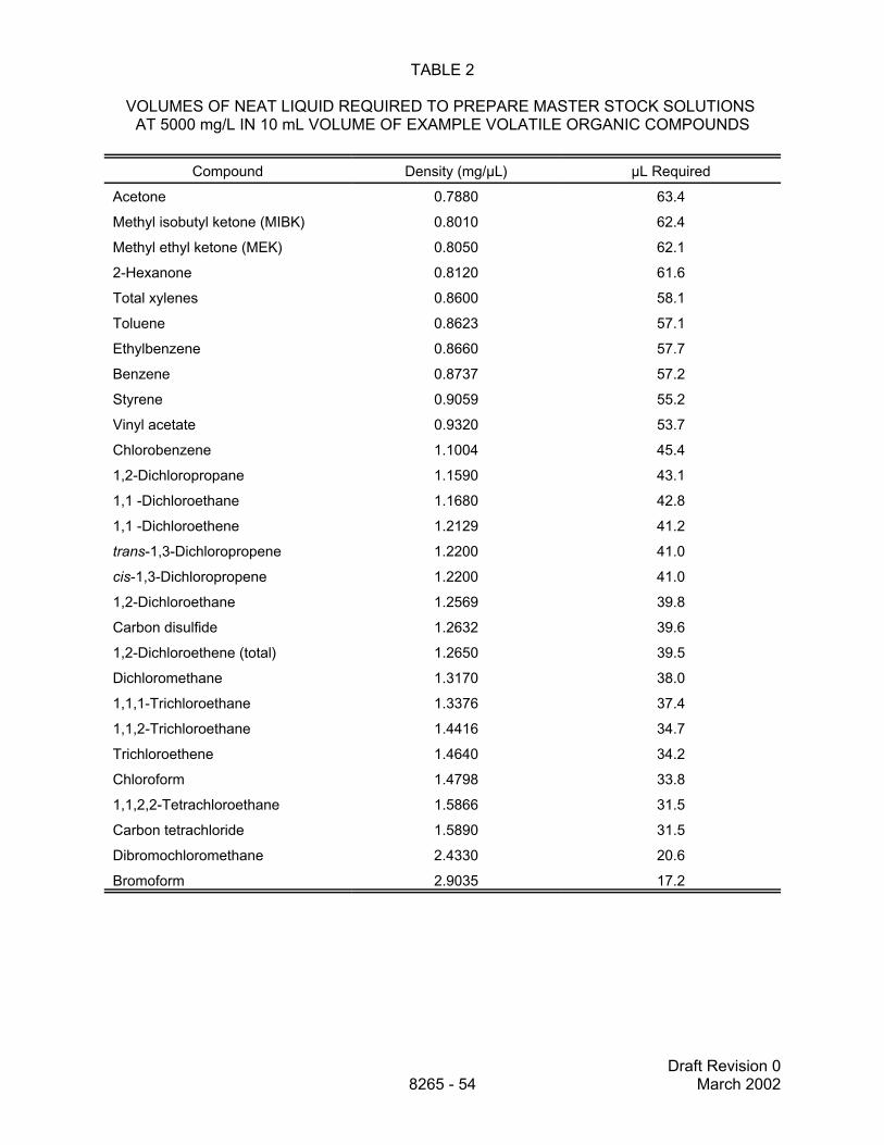
Draft Revision 0March 20028265 - 54
TABLE 2
VOLUMES OF NEAT LIQUID REQUIRED TO PREPARE MASTER STOCK SOLUTIONS AT 5000 mg/L IN 10 mL VOLUME OF EXAMPLE VOLATILE ORGANIC COMPOUNDS
Compound Density (mg/µL) µL Required
Acetone 0.7880 63.4
Methyl isobutyl ketone (MIBK) 0.8010 62.4
Methyl ethyl ketone (MEK) 0.8050 62.1
2-Hexanone 0.8120 61.6
Total xylenes 0.8600 58.1
Toluene 0.8623 57.1
Ethylbenzene 0.8660 57.7
Benzene 0.8737 57.2
Styrene 0.9059 55.2
Vinyl acetate 0.9320 53.7
Chlorobenzene 1.1004 45.4
1,2-Dichloropropane 1.1590 43.1
1,1 -Dichloroethane 1.1680 42.8
1,1 -Dichloroethene 1.2129 41.2
trans-1,3-Dichloropropene 1.2200 41.0
cis-1,3-Dichloropropene 1.2200 41.0
1,2-Dichloroethane 1.2569 39.8
Carbon disulfide 1.2632 39.6
1,2-Dichloroethene (total) 1.2650 39.5
Dichloromethane 1.3170 38.0
1,1,1-Trichloroethane 1.3376 37.4
1,1,2-Trichloroethane 1.4416 34.7
Trichloroethene 1.4640 34.2
Chloroform 1.4798 33.8
1,1,2,2-Tetrachloroethane 1.5866 31.5
Carbon tetrachloride 1.5890 31.5
Dibromochloromethane 2.4330 20.6
Bromoform 2.9035 17.2

Draft Revision 0March 20028265 - 55
TABLE 3
VOLUME OF ANALYTE MASTER STANDARD INJECTED INTO A 10-L TEDLAR BAG TOPRODUCE ANALYTE WORKING STANDARDS FOR MEASUREMENT OF VOCs IN AIR
Target VOC Concentration (ppbv)Volume (mL) of Analyte Master Standard
Required for 10 L of Air
0 0.0 10 0.1 50 0.5 250 2.5 500 5.0
1,000 10.0
TABLE 4
BASIC ION TRAP SCAN FUNCTION FOR GENERATING ALTERNATING EI/CI MASSSPECTRA
Acquire electron ionization (EI) mass spectrumEvent Instrument Function
1 Reset and zero the scan parameters2 Electron ionization (store all ions >40 Daltons)3 Turn on the electron multiplier4 Scan the mass spectrum and acquire data to the computer
Acquire chemical Ionization (CI) mass spectrum5 Reset and zero the scan parameters6 Ionize Cl reagent by electron ionization (Store all ions >15 Daltons)7 Eject ions >25 Daltons8 Allow Cl reagent to react with analytes for 10-200 msec9 Turn on the multiplier
10 Scan the mass spectrum and acquire data to the computer11 Reset all scan parameters and return to event #1
*Note: The scan function listed above depicts the basic operations that occur within an ion trapmass spectrometer during the acquisition of alternating scans generated using electron ionization (EI) andchemical ionization (CI). It is assumed in the above a case that the CI reagent used is water vapor. Thisscan function is generic for most ion trap mass spectrometers although the software and hardware meansof implementing these scans is dependent on the manufacturer and specific model of the instrument. Referto the instrument operating manual for specific information regarding setup and operation.
Source: References 1 and 10.

Draft Revision 0March 20028265 - 56
TABLE 5
VOLUME OF ANALYTE WORKING SOLUTION INJECTED INTO 40 mL OF WATER TOOBTAIN A SOLUTION CONCENTRATION IN THE RANGE OF 0 TO 1,000 µg/L
Final Solution Concentration (µg/L)Volume (µL) of Analyte Working
Solution Injected into 40 mL of Water
0 0.0
2 0.8
5 2.0
15 6.0
25 10.0
50 20.0
100 40.0
250 100.0
500 200.0
1,000 400.0

Draft Revision 0March 20028265 - 57
TABLE 6
EXAMPLE METHOD QUANTITATION LIMITSa FOR EXAMPLE VOCs IN WATER AND AIR
CompoundWater (ppb)b Air (ppbv)b
EIc CIc EIc CIc
Acetone -d 2.3 - 12
Benzene 1.3 1.7 21 42
Bromodichloromethane 2.5 - 3 -
Bromoform 2.0 - 58 -
Bromomethane 2.4 - 53 -
Carbon disulfide 1.5 - 3 -
Carbon tetrachloride 1.3 - 5 -
Chlorobenzene 0.5 1.4 16 12
Chloroethane 3.2 - 17 -
Chloroform 1.5 - 17 -
Chloromethane 4.7 - - -
Dibromochloromethane 4.4 - 4 -
1,1-Dichloroethane 3.0 - 8 -
1,2-Dichloroethane 1.5 - 12 -
1,1-Dichloroethene 2.0 2.6 14 -
cis-1,2-Dichloroethene 2.5 - 11 -
trans-1,2-Dichloroethene 1.7 - 12 -
Dichloromethane 3.0 - 17 -
1,2-Dichloropropane 3.2 - 10 -
cis-1,3-Dichlororopene 2.2 2.0 2 -
trans-1,3-Dichloropropene 1.9 1.5 3 -
Ethylbenzene 1.3 1.4 21 14
2-Hexanone - 2.1 104 35
Methyl ethyl ketone (MEK) - 3.2 37 46
Methyl isobutyl ketone (MIBK) - 2.6 33 16
Styrene 0.5 0.9 13 12(continued)

Draft Revision 0March 20028265 - 58
TABLE 6(Continued)
CompoundWater (ppb)b Air (ppbv)b
EIc CIc EIc CIc
1,1,2,2-Tetrachloroethane 2.1 - 27 -
Tetrachloroethene 1.3 - 12 -
Toluene 0.5 0.5 4 6
1,1,1-Trichloroethane 0.6 - 15 -
1,1,2-Trichloroethane 3.3 - 5 -
Trichloroethene 2.7 - 6 -
Vinyl acetate - 3.3 61 -
Vinyl chloride 1.0 - - -
Xylenes 0.8 1.9 9 8
a Calculated using the detection limit algorithm based on the linear regression line from experimentallydetermined calibration curves (4 points 2.5 to15 ppb for water, 50 to 500 ppbv for air for the data presented)under a single set of operating conditions. Conditions may be optimized to provide improved limits for anygiven analyte.
b Water by 40-mL vial purge. Air by real-time sampling from Tedlar bag.
c EI: Electron impact ionization. CI: Water chemical ionization.
d Not determined.
Source: References 3 and 9.

Draft Revision 0March 20028265 - 59
TABLE 7
EXAMPLE DSITMS PERFORMANCE EVALUATION (40-mL PURGE/WATER)a
VOC
TargetConc.(ppb) N
FoundMeanConc. (ppb)
Accuracy Precision
BiasbPercent Bias
StandardDeviation
%Coefficient
ofVariationc
Carbon tetrachloride
5 5 5.00 0.00 ± 0.34 0.0 0.275 5.5
10 6 9.42 -0.58 ± 0.39 -5.8 0.373 4.0
40 6 39.18 -0.82 ± 1.32 -2.0 1.259 3.2
Tetrachloroethene
5 5 5.20 0.20 ± 0.89 4.0 0.719 13.8
10 6 8.72 -1.28 ± 0.49 -12.8 0.466 5.3
40 6 35.92 -4.08 ± 1.25 -10.2 1.189 3.3
Trichloroethene
5 5 4.97 -0.03 ± 0.18 -0.6 0.148 3.0
10 6 9.45 -0.55 ± 0.42 -5.5 0.402 4.3
40 6 39.17 -0.83 ± 1.11 -2.1 1.061 2.7
N = Number of samples
a 40-mL purge of spiked ASTM groundwater over three week period.
b Bias = (Mean - Target Conc.) ± (t)(S)/%N Where S = Standard Deviation; t = Students t-Value for 95% Confidence; %N = square root of numberof samples
c % Coefficient of Variation = (S/Mean)(100%)
Source: Reference 11.
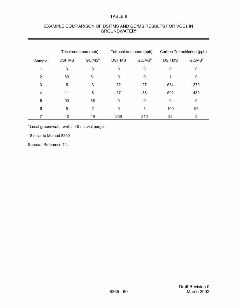
Draft Revision 0March 20028265 - 60
TABLE 8
EXAMPLE COMPARISON OF DSITMS AND GC/MS RESULTS FOR VOCs INGROUNDWATERa
Sample
Trichloroethene (ppb) Tetrachloroethene (ppb) Carbon Tetrachloride (ppb)
DSITMS GC/MSb DSITMS GC/MSb DSITMS GC/MSb
1 3 3 0 0 0 0
2 89 81 0 0 1 0
3 5 3 32 27 634 370
4 11 8 57 38 592 430
5 90 56 0 0 0 0
6 5 2 9 8 100 93
7 40 49 256 210 32 5
a Local groundwater wells. 40-mL vial purge.
b Similar to Method 8260
Source: Reference 11.

Draft Revision 0March 20028265 - 61
TABLE 9
EXAMPLE COMPARISON OF RESULTS FOR GASOLINE RANGE ORGANICS (GRO) IN WATER
Sample IDGRO Concentration (ppb)
DSITMSa GC/FID
193 2598 2400
708 8828 6400
657 < 5 < 100
707 < 5 < 100
808 < 5 < 100
810 13 < 100
204 172 150
656b 368b 2300b
806 24 160
632 7538 8200
508 35933 58000a Measured using m/z 56 plus 57.
b Contaminated with carbon tetrachloride and trichloroethene.
Source: Reference 9.
TABLE 10
EXAMPLE COMPARISON OF DSITMS RESULTS WITH LABORATORY RESULTS FORSOLVENTS IN GROUNDWATER BY IN-SITU SPARGE
SampleTrichloroethene (µg/L) Tetrachloroethene (µg/L)
Lab 1a Lab 2a DSITMSb Lab 1a Lab 2a DSITMSb
1 56 74 88 34 43 49
2 18 19 15 22 23 20
3 40 50 60 70 383 298
aEPA Method 5030/8260
bIn-situ hydrosparge
Source: Reference 4.

Draft Revision 0March 20028265 - 62
TABLE 11
EXAMPLE PERFORMANCE EVALUATION CHECK STANDARDS BY IN-SITU SPARGE
DayEPA VOA
nominal (µg/L)Hydrosparge (µg/L)
DCE TCE
1 40 38 29
2 16 18 14
3 100 83 112
3 16 16 15
4 72 87 75
5 100 134 109
5 350 302 343
6 40 67 44
7 20 36 20
8 20 29 19
Source: Reference 12.

Draft Revision 0March 20028265 - 63
TABLE 12
EXAMPLE SPIKE RECOVERIES OF BTEXa FROM SOILb USING DSITMS
Sample
Spike Recovery (%)
Benzene Toluene EtBz + Xyl
1 64 74 64
2 70 82 54
3 60 52 48
4 50 62 58
5 78 64 56
Mean 64.4 66.8 56
Std Dev 10.5 11.5 5.8
aBenzene, toluene, ethylbenzene, plus xylenes.
bRoom temperature purge of local soil spiked at 400 ng/g versus purge of pH 7 water.
Source: Reference 9.
TABLE 13
EXAMPLE OF THERMAL DESORPTION DSITMS RESULTS FOR NICOTINE IN AIR
Nicotine (µg/m3)
Samplea DSITMS Reference Method
1 0.82 0.45
2 27 18
3 122 123
4 141 178
5 361 260
aCollected on solid sorbent trap
Source: Reference 9.

Draft Revision 0March 20028265 - 64
FIGURE 1
CAPILLARY RESTRICTOR INTERFACE WITH OPEN-SPLIT INLET AND QUICK-CONNECT FITTING FOR THE ATTACHMENTOF SAMPLE INTRODUCTION MODULES AND SAMPLE ARCHIVAL SORBENT TRAPS