Method 1611.1: Enterococci in Water by TaqMan® Quantitative Polymerase Chain Reaction (qPCR)

April 2015

1

U.S. Environmental Protection Agency Office of Water (4303T)

1200 Pennsylvania Avenue, NW Washington, DC 20460

EPA-820-R-15-008

Method 1611.1

Acknowledgments This method was developed under the direction of Rich Haugland, Kevin Oshima and Alfred P. Dufour of the U.S. Environmental Protection Agency’s (EPA) Human Exposure Research Division, National Exposure Research Laboratory, Cincinnati, Ohio. The following laboratories are gratefully acknowledged for their participation in the multi-laboratory validation of this method in fresh and marine waters: Participant Laboratories Single Laboratory Validation

• Mycometrics, LLC: King-Teh Lin and Pi-shiang Lai • New York State Department of Health, Environmental Biology Laboratory: Ellen Braun-

Howland and Stacey Chmura

• Marine ambient water multi-laboratory validation: BioVir: Rick Danielson and Rosie Newton • EPA Region 1 – New England Regional Laboratory: Jack Paar and Mark Doolittle • EPA Region 10 Laboratory: Barry Pepich and Stephanie Harris • Hampton Roads Sanitation District: Robin Parnell and Tiffany Elston • King County Environmental: Eric Thompson and Joe Clark • Mycometrics: King-Teh Lin and Rose Lee • NOAA – AOML/Ocean Chemistry Division: Chris Sinigalliano, David Wanless, and Maribeth

Gidley • NOAA – NOS/Center for Coastal Environmental Health & Biomolecular Research: Janet Gooch

Moore and Chris Johnston • Orange County Public Health Laboratory: Richard Alexander and Joe GuzmanTexas A&M

University – Corpus Christi: Joanna Mott, Ladonna Henson, Sarah Bortz, and Lindsey Myers • Virginia Institute of Marine Science: Howard Kator and Kimberly Reece

Fresh ambient water multi-laboratory validation:

• BioVir: Rick Danielson and Rosie Newton • Hampton Roads Sanitation District: Robin Parnell and Tiffany Elston • King County Environmental: Eric Thompson and Joe Clark • Orange County Public Health Laboratory: Richard Alexander and Joe Guzman • Orange County Water District: Donald Phipps and Menu Leddy • Scientific Methods Incorporated: Fu-Chih Hsu and Rebecca Wong

• Texas A&M University – Corpus Christi: Joanna Mott, Ladonna Henson, and Sarah Bortz • Texas A&M University – College Station: Suresh Pillai and Charlotte Rambo • University of Iowa Hygienic Lab: Nancy Hall, Greg Gingerich, and Lucy DesJardin • Wisconsin State Lab of Hygiene: Sharon Kluender and Jeremy Olstadt

i

Method 1611.1

Disclaimer Neither the United States Government nor any of its employees, contractors, or their employees make any warranty, expressed or implied, or assumes any legal liability or responsibility for any third party’s use of apparatus, product, or process discussed in this method, or represents that its use by such a party would not infringe on privately owned rights. Mention of trade names or commercial products does not constitute endorsement or recommendation for use. Questions concerning this method or its application should be addressed to: Robin K. Oshiro Engineering and Analysis Division (4303T) U.S. EPA Office of Water, Office of Science and Technology 1200 Pennsylvania Avenue, NW Washington, DC 20460 oshiro.robin@epa.gov or OSTCWAMethods@epa.gov

ii

Method 1611.1

Introduction Enterococci are commonly found in the feces of humans and other warm-blooded animals. Although these organisms can be persistent in the environment, the presence of enterococci in water is an indication of fecal pollution and the possible presence of enteric pathogens. Epidemiological studies have led to the development of criteria for promulgating recreational water standards based on established relationships between the measured density of enterococci colony forming units (CFUs) in the water by culture based methods and the risk of gastrointestinal illness associated with swimming in the water (References 16.3, 16.8, 16.9, 16.10, and 16.11). Method 1611.1 describes a quantitative polymerase chain reaction (qPCR) procedure for the detection of DNA from enterococci bacteria in ambient water matrices based on the amplification and detection of a specific region of the large subunit ribosomal ribonucleic acid (RNA) gene (lsrRNA, 23S rRNA) from these organisms. The advantage of Method 1611.1 over currently accepted culture methods that require 24 - 48 hours to obtain results is its relative rapidity. Results can be obtained by Method 1611.1 in 3 - 4 hours, allowing same-day notification of recreational water quality. In Method 1611.1, water samples are filtered to collect enterococci on polycarbonate membrane filters. Following filtration, total deoxyribonucleic acid (DNA) is solubilized from the filter retentate using a bead beater. Enterococci target DNA sequences present in the clarified homogenate are detected by the real-time quantitative polymerase chain reaction (qPCR) technique using TaqMan® Universal master mix PCR reagent and the TaqMan® probe system. The TaqMan® system signals the formation of PCR products by a process involving enzymatic hydrolysis of a fluorogenically labeled oligonucleotide probe when it hybridizes to the target sequence. Method 1611.1 uses an arithmetic formula, the comparative cycle threshold (CT) method, to calculate the ratio of Enterococcus lsrRNA gene copies (target sequences) recovered in total DNA extracts from water samples relative to those in similarly prepared extracts of calibrator samples containing a known quantity of Enterococcus cells. The target sequence ratio can be multiplied by the number of Enterococcus cells in the calibrator sample to obtain estimates of calibrator cell equivalents (CCE) in the water samples. The absolute quantity of target sequences in the calibrator sample extracts can also be determined and used in the comparative CT method to obtain estimates of the target sequence copies or, together with Enterococcus cell numbers in the calibrator sample, to obtain CCE estimates with associated defined target sequences per CCE in the water samples. CT values for sample processing control (SPC) sequences added in equal quantities to both the water filtrate and calibrator samples before DNA extraction are used to normalize results for potential differences in DNA recovery or to signal inhibition or fluorescence quenching of the PCR analysis caused by a sample matrix component or possible technical error. In addition, an internal amplification control (IAC) is added to each qPCR analysis for Enterococcus DNA and is co-amplified simultaneously with the target sequence; to specifically identify polymerase inhibition in the reactions.

iii

Method 1611.1

Table of Contents

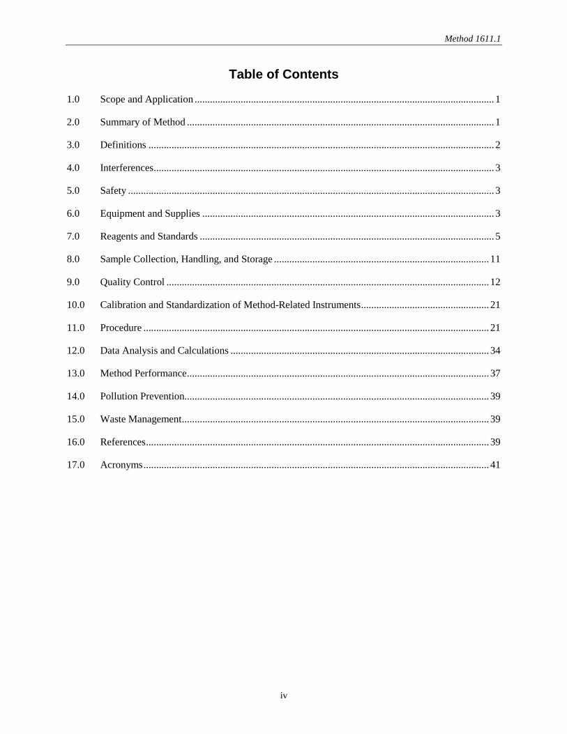
1.0 Scope and Application ..................................................................................................................... 1

2.0 Summary of Method ........................................................................................................................ 1

3.0 Definitions ....................................................................................................................................... 2

4.0 Interferences ..................................................................................................................................... 3

5.0 Safety ............................................................................................................................................... 3

6.0 Equipment and Supplies .................................................................................................................. 3

7.0 Reagents and Standards ................................................................................................................... 5

8.0 Sample Collection, Handling, and Storage .................................................................................... 11

9.0 Quality Control .............................................................................................................................. 12

10.0 Calibration and Standardization of Method-Related Instruments .................................................. 21

11.0 Procedure ....................................................................................................................................... 21

12.0 Data Analysis and Calculations ..................................................................................................... 34

13.0 Method Performance ...................................................................................................................... 37

14.0 Pollution Prevention....................................................................................................................... 39

15.0 Waste Management ........................................................................................................................ 39

16.0 References ...................................................................................................................................... 39

17.0 Acronyms ....................................................................................................................................... 41

iv

Method 1611.1

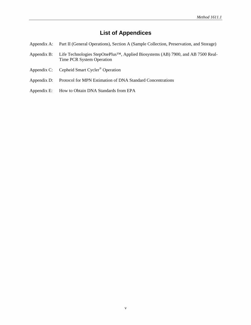
List of Appendices Appendix A: Part II (General Operations), Section A (Sample Collection, Preservation, and Storage) Appendix B: Life Technologies StepOnePlus™, Applied Biosystems (AB) 7900, and AB 7500 Real-

Time PCR System Operation Appendix C: Cepheid Smart Cycler® Operation Appendix D: Protocol for MPN Estimation of DNA Standard Concentrations Appendix E: How to Obtain DNA Standards from EPA

v

Method 1611.1

Method 1611.1: Enterococci in Water by Quantitative Polymerase Chain Reaction (qPCR)

April 2015

1.0 Scope and Application 1.1 Method 1611.1 describes a qPCR procedure for the measurement of large subunit ribosomal RNA

(lsrRNA, 23S rRNA) target gene sequences (target sequences) from all known species of enterococci bacteria in water. This method is based on the collection of enterococci on membrane filters, extraction of total DNA using a bead beater, and detection of enterococci target sequences in the supernatant by real-time polymerase chain reaction (PCR) using TaqMan® Universal master mix PCR reagent and the TaqMan® probe system. The TaqMan® system signals the formation of PCR products by a process involving the enzymatic hydrolysis of a labeled fluorogenic probe that hybridizes to the target sequence.

1.2 The Method 1611.1 test is recommended as a measure of ambient marine and fresh recreational

water quality. The significance of finding Enterococci DNA target sequences in recreational water samples stems from the association between the density of these sequences and the reported occurrence of gastrointestinal (GI) illness associated with swimming observed in recent epidemiological studies (References 16.11, 16.13, and 16.14).

1.3 The variable recoveries observed during the validation studies should be taken into consideration

when analyzing results from Method 1611.1. Guidance is provided in Section 9 of this document on how laboratories can monitor the initial and ongoing performance of the method in their hands. It is expected and has been observed that the performance of the method will improve as laboratories gain additional experience with it through continued practice.

1.4 This method assumes the use of an Applied Biosystems (AB) Sequence Detector as the default platform. (Note: Applied Biosystems is now Life Technologies). The Cepheid Smart Cycler® may also be used. The user should refer to the platform specific instructions for these instruments in the appendices. Users should thoroughly read the method in its entirety before preparation of reagents and commencement of the method to identify differences in protocols for different platforms.

2.0 Summary of Method The method is initiated by filtering a water sample through a membrane filter. Following

filtration, the membrane containing the bacterial cells and DNA is placed in a microcentrifuge tube with glass beads and buffer, and then shaken at high speed to extract the DNA into solution. The supernatant is used for PCR amplification and detection of target sequences using the TaqMan® Universal master mix PCR reagent and probe system.

1

Method 1611.1

3.0 Definitions 3.1 Enterococci: all species of the genus Enterococcus for which lsrRNA gene nucleotide sequences

were reported in the GenBank database (http://www.ncbi.nlm.nih/gov/Genbank) at the time of method development.

3.2 Target sequence: An approximately 94 base pairs (bp) segment of the Enterococcus lsrRNA gene

containing nucleotide sequences that are homologous to both the primers and probe used in the Enterococcus qPCR assay and that is common only to species within this genus.

3.3 Sample processing control (SPC) sequence: A 77 bp segment of the ribosomal RNA gene operon,

internal transcribed spacer region 2 of chum salmon, Oncorhynchus keta (O. keta) and other salmon spp., containing nucleotide sequences that are homologous to the primers and probe used in the SPC qPCR assay. SPC sequences are added as part of a total salmon DNA solution in equal quantities to all water sample filtrate and calibrator samples prior to extracting DNA from the samples. The purpose of this control is to determine whether the sample was processed correctly and/or to identify and correct for sample matrix effects on total DNA recovery (as described in Section 9.12).

3.4 DNA standard: A purified, RNA-free and quantified and characterized Enterococcus faecalis (E.

faecalis) strain ATCC® 29212™ genomic DNA preparation. Note: DNA standards are used to generate standard curves for determination of performance characteristics of the qPCR assays and instrument with different preparations of master mixes containing TaqMan® reagent, primers and probe as described in Section 9.10. Also used for quantifying target sequences in calibrator sample extracts as described in Section 12.4.

3.5 Calibrator sample: Samples containing defined added quantities of E. faecalis strain ATCC®

29212™ cells and SPC sequences that are extracted and analyzed in the same manner as water sample filtrates. Calibrator sample analysis results are used as positive controls for the Enterococcus target sequence and SPC qPCR assays and as the basis for target sequence quantification in water sample filtrates using the ΔΔCT comparative cycle threshold calculation method (ΔΔCT method) as described in Section 12.5. Analysis results of these samples provide corrections for potential daily or weekly method-related variations in Enterococcus cell lysis, target sequence recovery and PCR efficiency. qPCR analyses for SPC sequences from these samples are also used to correct for variations in total DNA recovery in the extracts of water sample filtrates that can be caused by contaminants in these filtrates, as described in Section 12.4, and/or to signal potentially significant PCR inhibition caused by these contaminants as described in Section 9.8.

3.6 ΔΔCT method: A calculation method derived by AB (Reference 16.1) for calculating the ratios of

target sequences in two DNA samples (e.g., a calibrator and water filtrate sample) that normalizes for differences in total DNA recovery from these samples using qPCR analysis CT (cycle threshold) values for a reference (SPC) sequence that is initially present in equal quantities prior to DNA extraction.

3.7 Amplification factor (AF): A measure of the average efficiency at which target or SPC sequences

are copied and detected by their respective primer and probe assays during each thermal cycle of the qPCR reaction that is used in the ΔΔCT method. AF values can range from 1 (0% of sequences copied and detected) to 2 (100% of sequences copied and detected) and are calculated from a standard curve as described in Section 12.3.

2

Method 1611.1

3.8 Internal amplification control (IAC): A non-target DNA sequence that is used to help specifically identify false negative reactions or reduced amplification efficiency due to Taq DNA polymerase inhibition. For an explanation of this type of PCR interference, see Sections 4.0 and 9.13.

4.0 Interferences

Water samples containing colloidal or suspended particulate materials can clog the membrane filter and prevent filtration. These materials can also interfere with the PCR analysis by inhibiting the enzymatic activity of the Taq DNA polymerase and/or by interfering with the annealing of the primer and probe oligonucleotides to sample target DNA, enzyme and/or by the quenching of hydrolyzed probe fluorescence and/or by reducing (or potentially facilitating) total DNA recovery.

5.0 Safety 5.1 The analyst/technician must know and observe the normal safety procedures required in a

microbiology and/or molecular biology laboratory while preparing, using, and disposing of cultures, reagents, and materials, and while operating sterilization equipment.

5.2 Where possible, facial masks should be worn to prevent sample contamination.

5.3 Mouth-pipetting is prohibited. 6.0 Equipment and Supplies 6.1 Separated, and dedicated workstations for reagent preparation and for sample preparation,

preferably with high efficiency particulate air (HEPA)-filtered laminar flow hoods and an Ultraviolet (UV) light source, each having separate supplies (e.g., pipettors, tips, gloves, etc.). Note: While not recommended, the same workstation may be used for the entire procedure provided that it has been cleaned with bleach and UV sterilized as specified in Section 11.8.1 between reagent and sample preparation. Under recommended conditions, the two dedicated workstations should be in separate rooms with unidirectional workflow (i.e., all reagents should be prepared before sample preparation and the reagent preparation room should not be re-entered after moving to the sample preparation room.

6.2 Balance capable of accuracy to 0.01 g

6.3 Extraction tubes: semi-conical, screw cap microcentrifuge tubes, 2.0 mL (e.g., Sarstedt D-51588 or equivalent)

6.4 Glass beads, acid washed, 212 - 300 μm (e.g., Sigma G-1277 or equivalent)

6.4.1 May also be purchased in extraction tubes from various commercial vendors (e.g., Gene-Rite S0205-50 or equivalent)

6.5 Autoclave, capable of achieving and maintaining 121°C [15 lb pounds per square inch (PSI)] for minimally 15 minutes (optional, Note: Avoid use of autoclaves that are routinely used for sterilizing biological materials. These autoclaves may contain target DNA contamination that has been generated by aerosolization of DNA from the previous materials. This DNA is not necessarily totally destroyed by the autoclaving process, and can contaminate your newly

3

Method 1611.1

sterilized materials. If a dedicated autoclave for sterilizing non-biological materials is not available, it may be preferable to either use disposable materials or sterilize reusable items with bleach and UV light treatment.)

6.6 Workstation for water filtrations, preferably a HEPA-filtered laminar flow hood with a UV light source. This can be the same as used for sample preparation, Section 6.1.

6.7 Sterile bottles/containers for sample collection

6.8 Membrane filtration units (filter base and funnel) for 47 mm diameter filters, sterile glass, plastic stainless steel, or disposable plastic (e.g., Pall Gelman 4242, Nalgene CN 130-4045,CN 145-0045, or equivalent), cleaned and bleach treated (rinsed with 10% v/v bleach, then 3 rinses with reagent-grade water), covered with aluminum foil or Kraft paper, and autoclaved or UV-sterilized if non-disposable

6.9 Line vacuum, electric vacuum pump, or aspirator for use as a vacuum source. In an emergency or in the field, a hand pump or a syringe equipped with a check valve to prevent the return flow of air can be used.

6.10 Flask, filter, vacuum, usually 1 L, with appropriate tubing

6.11 Filter manifold to hold a number of filter bases

6.12 Flask for safety trap placed between the filter flask and the vacuum source 6.13 Forceps, straight or curved, with smooth tips to handle filters without damage, 2 pairs

6.14 Polycarbonate membrane filters, sterile, white, 47 mm diameter, with 0.45 μm pore size (e.g., Millipore HTTP04700 or equivalent) 6.14.1 May also be purchased in sterile single use membrane filter units from various

commercial vendors (e.g., Pall FMFNL 1050 or equivalent) 6.15 Graduated cylinders, 100 - 1000 mL, cleaned and bleach treated (rinsed with 10% v/v bleach,

then 3 rinses with reagent-grade water), covered with aluminum foil or Kraft paper and autoclaved or UV-sterilized

6.16 Petri dishes, sterile, plastic or glass, 100 × 15 mm with loose fitting lids

6.17 Disposable loops, 1 μL and 10 μL

6.18 Permanent ink marking pen for labeling tubes

6.19 Visible wavelength spectrophotometer capable of measuring at 595 nm 6.20 Single or multi-place bead beater (e.g., Biospec Products Inc. 3110BX or equivalent).

6.21 Microcentrifuge capable of 12,000 × g 6.22 Micropipettors with 10, 20, 200 and 1000 μL capacity. Under ideal conditions, each workstation

should have a dedicated set of micropipettors (one micropipettor set for pipetting reagents not containing cells or DNA and one set for reagents containing DNA and test samples).

6.23 Micropipettor tips with aerosol barrier for 10, 20, 200 and 1000 μL capacity micropipettors. Note: All micropipetting should be done with aerosol barrier tips. The tips used for reagents not containing DNA should be separate from those used for reagents containing DNA and test samples. Each workstation should have a dedicated supply of tips.

6.24 Microcentrifuge tubes, low retention, clear, 1.7 mL (e.g., GENE MATE C-3228-1 or equivalent) 6.25 Test tube rack for microcentrifuge tubes

6.26 Graduated conical centrifuge tubes, sterile, screw cap, 50 mL

4

Method 1611.1

6.27 Test tubes, screw cap, borosilicate glass, 16 × 125 mm

6.28 Pipet containers, stainless steel, aluminum or borosilicate glass, for glass pipets 6.29 Pipets, sterile, T.D. bacteriological or Mohr, disposable glass or plastic, of appropriate volume

(disposable pipets preferable) 6.30 Vortex mixer (ideally one for each work station)

6.31 Dedicated lab coats for each work station

6.32 Disposable powder-free gloves for each work station

6.33 Refrigerator, 4°C (ideally one for reagents and one for DNA samples)

6.34 Freezer, -20°C and/or -80°C (ideally, one for reagents and one for DNA samples)

6.35 Ice, crushed or cubes for temporary preservation of samples and reagents 6.36 Printer (optional)

6.37 Data archiving system (e.g., flash drive or other data storage system) 6.38 UV spectrophotometer capable of measuring wavelengths of 260 and 280 nm using small volume

capacity (e.g., 0.1 mL) cuvettes or NanoDrop® (ND-2000) spectrophotometer (or equivalent) capable of the same measurements at 2 μL sample volumes

6.39 Life Technologies StepOnePlus™, or AB 7500 Real-Time PCR System

6.39.1 Optical 96 well PCR reaction tray (e.g., Life Technologies MicroAmp™ 4346906 or equivalent)

6.39.2 Optical adhesive PCR reaction tray tape (e.g., Life Technologies MicroAmp™ 4311971 or equivalent) or MicroAmp™ caps (e.g., Applied Biosystems N8010534 or equivalent)

6.39.3 Life Technologies StepOnePlus™, AB 7900, or AB 7500 Real-Time PCR System

6.40 Cepheid Smart Cycler® (optional to Section 6.39) 6.40.1 Smart Cycler® 25 μL PCR reaction tubes (e.g., Cepheid 900-0085 or equivalent)

6.40.2 Rack and microcentrifuge for Smart Cycler® PCR reaction tubes. Note: Racks and microcentrifuge are provided with the Smart Cycler® thermocycler

6.40.3 Cepheid Smart Cycler® System thermocycler 7.0 Reagents and Standards

Note: The E. faecalis stock culture (Section 7.8), Salmon DNA/extraction buffer (Section 7.12), and DNA extraction tubes (Section 7.18), may be prepared in advance.

7.1 Purity of Reagents: Use molecular grade reagents and chemicals in all tests 7.2 Control Culture

• E. faecalis ATCC® 29212™ May also be purchased in a quantified form from commercial vendors (e.g., bioMerieux 56005)

7.3 SPC DNA (source of SPC control sequences) • Salmon testes DNA (e.g., Sigma D1626 or equivalent)

7.4 Phosphate Buffered Saline (PBS)

5

Method 1611.1

7.4.1 Composition:

Component Amount

Monosodium phosphate (NaH2PO4) 0.58 g

Disodium phosphate (Na2HPO4) 2.50 g

Sodium chloride 8.50 g

Reagent-grade water 1.0 L

7.4.2 Dissolve reagents in 1 L of reagent-grade water in a flask and dispense in appropriate amounts for dilutions in screw cap bottles or culture tubes, and/or into containers for use as rinse water. Autoclave after preparation at 121°C (15 PSI) for 15 minutes. Final pH should be 7.4 ± 0.2.

7.4.3 May also be purchased pre-made from various commercial vendors (e.g., Fisher Scientific BP2438-4 or equivalent)

7.5 Brain heart infusion broth (BHIB)

7.5.1 Composition:

Component Amount

Calf brains, infusion from 200.0 g 7.7 g

Beef heart, infusion from 250.0 g 9.8 g

Proteose peptone 10.0 g

Sodium chloride 5.0 g

Disodium phosphate (Na2HPO4) 2.5 g

Dextrose 2.0 g

Reagent-grade water 1.0 L 7.5.2 Add reagents to 1 L of reagent-grade water, mix thoroughly, and heat to dissolve

completely. Dispense 10 mL volumes in screw cap 16 × 125 mm tubes and autoclave at 121°C (15 PSI) for 15 minutes. Final pH should be 7.4 ± 0.2.

7.5.3 Dry reagents may also be purchased pre-mixed from various commercial vendors (e.g., BactoTM Brain Heart Infusion, Difco-BBL 237400 or equivalent) and dissolved with water and sterilized as in Section 7.5.2.

7.6 Brain heart infusion agar (BHIA) 7.6.1 Composition:

BHIA contains the same components as BHIB with the addition of 15.0 g agar per liter of BHI broth.

7.6.2 Add agar to formula for BHIB provided above. Prepare as in Section 7.5.2. After sterilization, dispense 12 - 15 mL into 100 × 15 mm petri dishes. Final pH should be 7.4 ± 0.2.

7.7 Sterile glycerol (used for preparation of E. faecalis stock culture as described in Section 7.8)

7.8 Preparation of E. faecalis (ATCC® 29212™) stock culture

Rehydrate lyophilized E. faecalis per manufacturer’s instructions (for ATCC® stocks, suspend in 5 - 6 mL of sterile BHIB and incubate at 37°C for 24 hours). Centrifuge for 5 minutes at

6

Method 1611.1

6000 × g to create a pellet. Using a sterile pipet, discard supernatant. Resuspend pellet in 10 mL of fresh sterile BHI broth containing 15% glycerol and dispense in 1.5 mL aliquots in microcentrifuge tubes. Freeze at -20°C (short term storage) or -80°C (long term storage). Note: Aliquots of suspension may be plated (Section 11.1) to determine colony forming unit (CFU) concentration. It is advisable to verify the E. faecalis culture as described, for example, in Section 15 of EPA Method 1600.

7.9 PCR-grade water (e.g., OmniPur 9602, EMD Chemicals 9610 or equivalent). Water must be DNA/DNase free.

7.10 Isopropanol or ethanol, 95%, for flame-sterilization

7.11 AE Buffer, pH 9.0 (e.g., Qiagen 19077 or equivalent) (Note: pH 8.0 is acceptable)

Composition: 10 mM Tris-Cl (Tris-chloride) 0.5 mM EDTA (Ethylenediaminetetraacetic acid) 7.12 Salmon DNA/extraction buffer

7.12.1 Composition:

Stock Salmon testes DNA (10 μg/mL) (Section 7.3) AE Buffer (Section 7.11)

7.12.2 Preparation of stock Salmon testes DNA: The recommended source of Salmon DNA is provided as a dried aggregate of purified high molecular weight genomic DNA. This material can be dissolved either in its entirety or a desired mass can be separated from the aggregate and dissolved. Add a volume in milliliters of AE buffer equal to the number of milligrams of DNA to be dissolved and stir, using a magnetic stir bar at low to medium speed, until dissolved (2 - 4 hours or longer, if necessary) followed by vigorous vortexing to obtain a homogeneous DNA solution. Dilute an aliquot of this solution to a concentration of ~ 10 μg/mL using AE buffer. Determine concentration of this solution by optical density at 260 (OD260) reading in a spectrophotometer. An OD260 of 0.2 is approximately equal to 10 μg/mL. This is your Salmon testes DNA working stock solution. Unused portions of the 1 mg/mL stock solution may be aliquoted and frozen at -20°C.

Note: For example, if the bottle contains 250 mg of dried DNA, add 250 mL AE buffer directly to the bottle. Cap tightly, and dissolve by at least 2 - 4 hours of gentle stirring followed by vigorous vortexing. The concentration should be about 1 mg/mL. Remove a 0.5 mL aliquot and dilute to 50 mL with AE buffer. The concentration should be about 10 µg/mL. Check absorbance (OD260) and calculate actual DNA concentration using the assumption that 1 OD260, unit is equivalent to 50 μg/mL DNA. Adjust this working stock to 10 μg/mL if necessary, either by further dilution or by adding additional 1 mg/mL stock, vortexing and rechecking OD260. Aliquot portions of the adjusted working DNA stock and store at 4°C in refrigerator.

7.12.3 Dilute Salmon testes DNA stock with AE buffer to make 0.2 μg/mL Salmon DNA/extraction buffer. Extraction buffer may be prepared in advance and stored at 4°C for a maximum of 1 week. Note: Determine the total volume of Salmon DNA/extraction buffer required for each day or week by multiplying volume (600 μL) × total number of samples to be analyzed including controls, water samples, and calibrator samples. For example, for 18 samples,

7

Method 1611.1

prepare enough Salmon/DNA extraction buffer for 24 extraction tubes [(18 ÷ 6 = 3, therefore, 3 extra tubes for water sample filtration blanks (method blanks) and 3 extra tubes for calibrator samples)]. Note that the number of samples is divided by 6 because you should conduct one method blank for every 6 samples analyzed. Additionally, prepare excess volume to allow for accurate dispensing of 600 μL per tube, generally 1 extra tube. Thus, in this example, prepare sufficient Salmon/DNA extraction buffer for 24 tubes plus one extra. The total volume needed is 600 μL × 25 tubes = 15,000 μL. Dilute the Salmon testes DNA working stock 1:50, for a total volume needed (15,000 μL) ÷ 50 = 300 μL of 10 μg/mL Salmon testes DNA working stock. The AE buffer needed is the difference between the total volume and the Salmon testes DNA working stock. For this example, 15,000 μL - 300 μL = 14,700 μL AE buffer needed.

7.13 Bleach solution: 10% v/v bleach (or other reagent that hydrolyzes DNA), used for cleaning work surfaces

7.14 Sterile water (used as rinse water for work surface after bleaching)

7.15 TaqMan® Universal PCR master mix 2.0 (e.g., Life Technologies 4304437 or equivalent)

7.16 Bovine serum albumin (BSA), fraction V powder (e.g., Sigma A-5611 or equivalent) Dissolve in PCR-grade water a concentration of 2 mg/mL.

7.17 Primer and probe sets: Primer and probe sets may be purchased from commercial sources. Primers should be desalted, probes should be HPLC (high-performance liquid chromatography) purified. 7.17.1 Enterococcus primer and probe set (Reference 16.4):

Forward primer: 5'-GAGAAATTCCAAACGAACTTG Reverse primer: 5'-CAGTGCTCTACCTCCATCATT TaqMan® probe: [6-FAM]-5'-TGGTTCTCTCCGAAATAGCTTTAGGGCTA-TAMRA

7.17.2 Salmon DNA primer and probe set (Reference 16.4):

Forward primer: 5'-GGTTTCCGCAGCTGGG Reverse primer: 5'-CCGAGCCGTCCTGGTC TaqMan® probe: [6-FAM]-5'-AGTCGCAGGCGGCCACCGT-TAMRA

7.17.3 Optional: Internal Amplification Control (IAC) primer and probe set (Reference 16.4) Primers: same as Enterococcus assay

UC1P1TaqMan® probe: [VIC]-5'-CCTGCCGTCTCGTGCTCCTCA-TAMRA Note: If using a Smart Cycler or other platforms that do not have channels for reading VIC reporter dye, TET may be substituted for VIC as the reporter dye.

7.17.4 Preparation of primer/probes: Using a micropipettor with aerosol barrier tips, add AE buffer to the lyophilized primers and probe from the vendor to create stock solutions of 500 μM primer and 100 μM probe and dissolve by extensive vortexing. Pulse centrifuge to coalesce droplets. (Note: Some vendors, i.e., AB/Life Technologies, provide probes already in solution at 100 μM concentration, part 450003). Store stock solutions at -20°C.

7.18 DNA extraction tubes Note: It is recommended that tube preparation be performed in advance of water sampling and

DNA extraction procedures.

8

Method 1611.1

Prepare 1 tube for each sample, and 1 extra tube for every 6 samples (i.e., for method blank) and minimum of 3 tubes per week for calibrator samples. Weigh 0.3 ± 0.01 g of glass beads (Section 6.4) and pour into extraction tube. Seal the tube tightly, checking to make sure there are no beads on the O-ring of the tube. Check the tube for proper O-ring seating after the tube has been closed. Optional: Autoclave tubes at 121°C (15 PSI) for 15 minutes.

7.19 Purified, RNA-free quantified and characterized E. faecalis genomic DNA preparations or commercial synthetic plasmid DNA for use as standards used to generate a standard curve (see Sections 11.2 and 11.5).

7.20 RNase A (e.g., Sigma Chemical R6513) or equivalent

7.20.1 Composition:

RNase A Tris-Cl NaCl

7.20.2 Dissolve 10 mg/mL pancreatic RNase A in 10 mM Tris-Cl (pH 7.5), 15 mM NaCl. Heat to 100°C for 15 minutes. Allow to cool to room temperature. Dispense into aliquots and store at -20°C. For working solution, prepare solution in PCR-grade water at concentration of 5 µg/µL.

7.21 DNA extraction kit (Gene-Rite K102-02C-50 DNA-EZ® RW02 or equivalent). (Note: This kit is not required if using BioBalls).

7.22 Restriction enzyme: plasmid vector dependent (e.g., Pvu I for pIDTsmart cloning vector provided by Integrated DNA Technologies or Hind III for pCR2.1 cloning vector provided by EurofinsMWG/Operon). Alternative enzyme and/or plasmid vector combinations may be chosen on the basis that the enzyme must have a single recognition site within the plasmid vector and no recognition sites within the inserted template sequence.

7.23 Optional: IAC (Reference 16.4)

Brief description: The IAC5 template contains interspersed sequences that are homologous to the forward and reverse primers of several qPCR assays including the Enterococcus qPCR assay used in Method 1611.1. Each primer pair produces a 111 bp amplicon from this template that contains the UC1P1 probe recognition sequence and is slightly longer than the corresponding native target sequence amplicon (see Section 3.2). The IAC5 template can be ordered as a custom-synthesized gene from commercial vendors. In this process the template sequence (see below) is synthesized in vitro, ligated with a plasmid vector chosen by the vendor (e.g., pIDTSMART-KAN, Integrated DNA Technologies, Coralville IA or pCR2.1, EurofinsMWG/Operon, Huntsville AL) and cloned into Escherichia coli. The recombinant plasmid is recovered, purified and lyophilized by the commercial provider.

Template sequencea,b: 5’-TCATGCAAGTCGAGCGATGGAGAAATTCCAAACGAACTTGGGGGTTCTGAGAGGAAGGTGGTAGAGCACTGTTTCGGCATCTGAGGAGCACGAGACGGCAGGCTCGAGAATGATGGAGGTAGAGCACTGAAAAGGAAGATTAATACCGCATAGAGAATGTTATCACGGGAGACAAGTAGCGTGAAGGATGACGG a Enterococcus forward and reverse primer recognition sequences underlined b UC1P1 probe recognition sequence in bold

9

Method 1611.1

7.23.1 Calculation of IAC concentrations

o Centrifuge tube briefly and dissolve lyophilized plasmid (IAC) in AE buffer to make a concentration of 20 µg/mL (e.g., 2 µg in 100 µL). Incubate at room temperature for 30 minutes and then vortex for 20 seconds.

o Check three, 2 µL aliquots of the dissolved plasmid for A260 and A280 absorbance using a spectrophotometer against an AE buffer blank and record average concentration. If the difference in expected and recorded concentrations is greater than 20% of expected (Table 1), stop protocol and recalculate dilutions provided in Table 2.

Table 1. Example Calculation of Stock Plasmid Concentration Molecular weight (from vendor) 1337095 Target sequence copy (TSC)/g: (avo # / mol. Wt) 4.50 × 1017 TSC/ng: molecules/g × 1×10-9 g/ng 4.50 × 108 Expected stock concentrations (ng/µL) 20 Expected stock TSC concentrations (TSC/µL) 9.01 × 109 Mean NanoDrop concentration

7.23.2 IAC linearization by restriction enzyme digestion

o Mix restriction enzyme buffer to make appropriate concentration (see Section 7.22 for enzyme choices and follow enzyme manufacturer’s instructions for selection and dilution of appropriate buffer) and 20 units of restriction enzyme and add PCR-grade water to achieve a final volume of 40 µL.

o Add 10 µL (or 200 ng equivalent volume) of dissolved IAC plasmid stock. (Note: Follow the manufacturer instructions, adjusting AE buffer volumes so that your final concentration is 2 x 104 TSC/µL.)

o Mix gently and incubate at 37ºC for 1 hour to digest DNA. o Dilute with AE buffer to bring the IAC/restriction enzyme digest volume up to 90

µL.

o In appropriately labeled 1.7 mL low retention microcentrifuge tubes, perform serial dilutions of the digested plasmid stock using AE buffer to achieve final digested plasmid DNA concentration 2 x 104 TSC/µL (2 × 10-5 dilution). Store digested plasmid stock and 2 × 10-1 - 2 × 10-4 dilutions at -80ºC. Store the 2 × 10-5 dilution in the refrigerator.

Table 2. Initial Dilution of Digested IAC Plasmid Stock IAC TSC/µL IAC TSC/2 µL Digested stock TSC concentrations: 1.0 × 109 2.0 × 109 Dilute 20 µL of stock w/80 µL AE (2 × 101 diln) 2.0 × 108 4.0 × 108 Dilute 100 µL of 2 × 10-1 diln w/ 900 µL AE (2 × 10-2 diln) 2.0 × 107 4.0 × 107 Dilute 100 µL of 2 × 10-2 diln w/ 900 µL AE (2 × 10-3 diln) 2.0 × 106 4.0 × 106 Dilute 100 µL of 2 × 10-3 diln w/ 900 µL AE (2 × 10-4 diln) 2.0 × 105 4.0 × 105 Dilute 100 µL of 2 × 10-4 diln w/ 900 µL AE (2 × 10-5 diln) 2.0 × 104 4.0 × 104

7.23.3 Preparation of IAC working stocks

o Perform serial dilutions of the 2 × 105 dilution to prepare working stocks as indicated in Table 3.

10

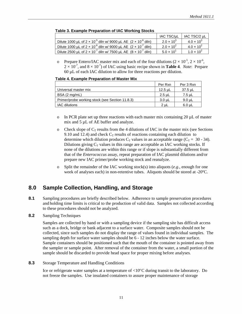
Method 1611.1

Table 3. Example Preparation of IAC Working Stocks IAC TSC/µL IAC TSC/2 µL Dilute 1000 µL of 2 × 10-5 diln w/ 9000 µL AE (2 × 10-6 diln) 2.0 × 103 4.0 × 103 Dilute 1000 µL of 2 × 10-6 diln w/ 9000 µL AE (2 × 10-7 diln) 2.0 × 102 4.0 × 102 Dilute 2500 µL of 2 × 10-7 diln w/ 7500 µL AE (8 × 10-7 diln) 5.0 × 101 1.0 × 102

o Prepare Entero/IAC master mix and each of the four dilutions (2 × 10-5, 2 × 10-6,

2 × 10-7, and 8 × 10-7) of IAC using basic recipe shown in Table 4. Note: Prepare 60 µL of each IAC dilution to allow for three reactions per dilution.

Table 4. Example Preparation of Master Mix Per Rxn Per 3 Rxn Universal master mix 12.5 µL 37.5 µL BSA (2 mg/mL) 2.5 µL 7.5 µL Primer/probe working stock (see Section 11.8.3) 3.0 µL 9.0 µL IAC dilutions 2 µL 6.0 µL

o In PCR plate set up three reactions with each master mix containing 20 µL of master mix and 5 µL of AE buffer and analyze.

o Check slope of CT results from the 4 dilutions of IAC in the master mix (see Sections 9.10 and 12.4) and check CT results of reactions containing each dilution to determine which dilution produces CT values in an acceptable range (CT = 30 - 34). Dilutions giving CT values in this range are acceptable as IAC working stocks. If none of the dilutions are within this range or if slope is substantially different from that of the Enterococcus assay, repeat preparation of IAC plasmid dilutions and/or prepare new IAC primer/probe working stock and reanalyze.

o Split the remainder of the IAC working stock(s) into aliquots (e.g., enough for one week of analyses each) in non-retentive tubes. Aliquots should be stored at -20ºC.

8.0 Sample Collection, Handling, and Storage

8.1 Sampling procedures are briefly described below. Adherence to sample preservation procedures

and holding time limits is critical to the production of valid data. Samples not collected according to these procedures should not be analyzed.

8.2 Sampling Techniques

Samples are collected by hand or with a sampling device if the sampling site has difficult access such as a dock, bridge or bank adjacent to a surface water. Composite samples should not be collected, since such samples do not display the range of values found in individual samples. The sampling depth for surface water samples should be 6 - 12 inches below the water surface. Sample containers should be positioned such that the mouth of the container is pointed away from the sampler or sample point. After removal of the container from the water, a small portion of the sample should be discarded to provide head space for proper mixing before analyses.

8.3 Storage Temperature and Handling Conditions

Ice or refrigerate water samples at a temperature of <10°C during transit to the laboratory. Do not freeze the samples. Use insulated containers to assure proper maintenance of storage

11

Method 1611.1

temperature. Ensure that sample bottles are tightly closed and are not totally immersed in water during transit.

8.4 Holding Time Limitations

Examine samples as soon as possible after collection. Do not hold samples longer than 6 hours between collection and initiation of filtration.

9.0 Quality Control

9.1 Each laboratory that uses Method 1611.1 is required to operate a formal quality assurance (QA) program that addresses and documents instrument and equipment maintenance and performance, reagent quality and performance, analyst training and certification, and records storage and retrieval. Additional recommendations for QA and quality control (QC) procedures for microbiological laboratories are provided in Reference 16.2.

9.2 The minimum analytical QC requirements for the analysis of samples using Method 1611.1 include an initial demonstration of laboratory capability through performance of initial DNA standard curve (Section 9.10) and calibrator sample analyses (Section 9.11) followed by initial precision and recovery (IPR) analyses (Section 9.3). Ongoing demonstration of laboratory capability should be demonstrated through performance of the ongoing precision and recovery (OPR) analysis (Section 9.4) and matrix spike (MS) analysis (Section 9.5), and the routine analysis of positive control (Section 9.6), no template controls (NTCs [Section 9.7]), method blanks (Section 9.8), media sterility checks (Section 9.9), DNA standard curves (Section 9.10), calibrator samples (Section 9.11), and SPCs (Section 9.12). For the IPR, OPR and MS analyses, it is necessary to spike samples with either laboratory-prepared spiking suspensions as described in Section 11.3 or BioBalls as described in Section 11.4.

9.3 Initial precision and recovery (IPR) — The IPR analyses are used to demonstrate acceptable method performance (recovery and precision) and should be performed by each laboratory before the method is used for monitoring field samples. An IPR should be performed by each analyst. The IPR analyses are performed as follows:

9.3.1 Prepare two or three calibrator samples and at least four reference (PBS) matrix spike samples with same number of cells as indicated in Section 11.3. Preparation of calibrator and reference (PBS) matrix spike samples with BioBalls is described in Section 11.4. Extract calibrator and reference (PBS) matrix spike samples as indicated in Section 11.3 and analyze as indicated in Sections 11.7 − 11.9. Calculate the calibrator cell equivalents (CCEs) in the reference (PBS) matrix spike samples according to Section 12. Note: Prepare calibrator samples from the same source of cells used to prepare the reference (PBS) matrix spike samples, i.e., for samples spiked with laboratory-prepared cell suspensions, use the same laboratory-prepared cell suspensions used to prepare calibrator samples; for samples spiked with BioBalls, use the same lot of BioBalls to prepare calibrator and reference (PBS) matrix spike samples.

9.3.2 Calculate the percent recovery (R) for each IPR sample according to the Method 1609.1/1611.1 Calculation Excel file.

9.3.3 Using the percent recoveries of the four analyses, calculate the mean percent recovery and the relative standard deviation (RSD) of the recoveries. The RSD is the standard deviation divided by the mean, multiplied by 100.

12

Method 1611.1

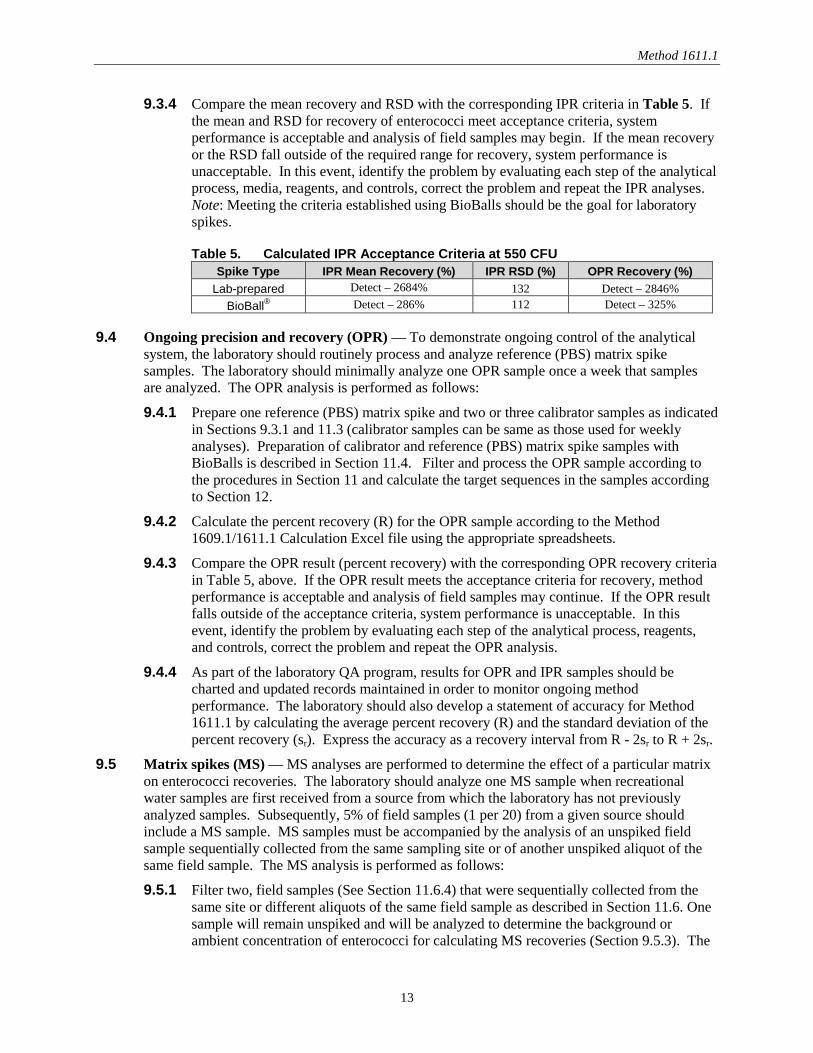
9.3.4 Compare the mean recovery and RSD with the corresponding IPR criteria in Table 5. If the mean and RSD for recovery of enterococci meet acceptance criteria, system performance is acceptable and analysis of field samples may begin. If the mean recovery or the RSD fall outside of the required range for recovery, system performance is unacceptable. In this event, identify the problem by evaluating each step of the analytical process, media, reagents, and controls, correct the problem and repeat the IPR analyses. Note: Meeting the criteria established using BioBalls should be the goal for laboratory spikes.

Table 5. Calculated IPR Acceptance Criteria at 550 CFU Spike Type IPR Mean Recovery (%) IPR RSD (%) OPR Recovery (%)

Lab-prepared Detect – 2684% 132 Detect – 2846% BioBall® Detect – 286% 112 Detect – 325%

9.4 Ongoing precision and recovery (OPR) — To demonstrate ongoing control of the analytical

system, the laboratory should routinely process and analyze reference (PBS) matrix spike samples. The laboratory should minimally analyze one OPR sample once a week that samples are analyzed. The OPR analysis is performed as follows:

9.4.1 Prepare one reference (PBS) matrix spike and two or three calibrator samples as indicated in Sections 9.3.1 and 11.3 (calibrator samples can be same as those used for weekly analyses). Preparation of calibrator and reference (PBS) matrix spike samples with BioBalls is described in Section 11.4. Filter and process the OPR sample according to the procedures in Section 11 and calculate the target sequences in the samples according to Section 12.

9.4.2 Calculate the percent recovery (R) for the OPR sample according to the Method 1609.1/1611.1 Calculation Excel file using the appropriate spreadsheets.

9.4.3 Compare the OPR result (percent recovery) with the corresponding OPR recovery criteria in Table 5, above. If the OPR result meets the acceptance criteria for recovery, method performance is acceptable and analysis of field samples may continue. If the OPR result falls outside of the acceptance criteria, system performance is unacceptable. In this event, identify the problem by evaluating each step of the analytical process, reagents, and controls, correct the problem and repeat the OPR analysis.

9.4.4 As part of the laboratory QA program, results for OPR and IPR samples should be charted and updated records maintained in order to monitor ongoing method performance. The laboratory should also develop a statement of accuracy for Method 1611.1 by calculating the average percent recovery (R) and the standard deviation of the percent recovery (sr). Express the accuracy as a recovery interval from R - 2sr to R + 2sr.

9.5 Matrix spikes (MS) — MS analyses are performed to determine the effect of a particular matrix on enterococci recoveries. The laboratory should analyze one MS sample when recreational water samples are first received from a source from which the laboratory has not previously analyzed samples. Subsequently, 5% of field samples (1 per 20) from a given source should include a MS sample. MS samples must be accompanied by the analysis of an unspiked field sample sequentially collected from the same sampling site or of another unspiked aliquot of the same field sample. The MS analysis is performed as follows:

9.5.1 Filter two, field samples (See Section 11.6.4) that were sequentially collected from the same site or different aliquots of the same field sample as described in Section 11.6. One sample will remain unspiked and will be analyzed to determine the background or ambient concentration of enterococci for calculating MS recoveries (Section 9.5.3). The

13

Method 1611.1

other sample will serve as the MS sample and will be spiked with E. faecalis ATCC® 29212™ according to the spiking procedure in Section 11.3 or Section 11.4 if using BioBalls. Note: For matrix spiking, filter the same volume as was filtered for the field samples.

9.5.2 Extract both the unspiked and spiked field samples according to the procedures in Section 11.7 and analyze in parallel with two or three calibrator sample extracts as described in Section 11.3 or Section 11.4 if using BioBalls.

9.5.3 For the MS sample, calculate the number of CCE and/or target sequences according to Section 12 and adjust based on any background enterococci CCE and/or target sequences calculated in the same manner in the unspiked matrix sample.

9.5.4 Calculate the percent recovery (R) for the MS sample (adjusted based on ambient enterococci in the unspiked sample) according to the Method 1609.1/1611.1 Calculation Excel File using the appropriate spreadsheets. Note: recovery results for sample containing ambient enterococci in the unspiked sample that are ≥ the spike density should be excluded from this analysis (Reference 16.12)

9.5.5 Compare the MS result (percent recovery) with the appropriate method performance criteria in Table 6. If the MS recovery meets the acceptance criteria, and system performance is acceptable, then analysis of field samples from this source may continue. If the MS recovery is unacceptable and the OPR sample result associated with this batch of samples is acceptable, a matrix interference may be causing the poor results. If the MS recovery is unacceptable, all associated field data should be flagged. Note: Meeting criteria established using BioBalls should also be a goal for laboratory spikes.

9.5.6 Laboratories should record and maintain a control chart comparing MS recoveries for all matrices to batch-specific and cumulative OPR sample results analyzed using Method 1611.1. These comparisons should help laboratories recognize matrix effects on method recovery and may also help to recognize inconsistent or sporadic matrix effects from a particular source.

Table 6. Calculated MS Precision and Recovery Acceptance Criteria at 550 CFU Matrix Spike Type MS Recovery (%) MS RPD 1 (%)

MW Lab-prepared Detect – 1198% 160

BioBall® Detect – 1123% 191

FW Lab-prepared Detect – 3473% 110

BioBall® Detect – 333% 354 1 Relative percent difference

9.6 Positive controls — The laboratory should analyze positive controls to ensure that the method is performing properly. Fluorescence amplification growth curve (PCR amplification trace) with an appropriate CT value during PCR indicates proper method performance. On an ongoing basis, the laboratory should perform positive control analyses every day that samples are analyzed. In addition, controls should be analyzed when new lots of reagents or filters are used.

9.6.1 Calibrator samples will serve as the positive control. Analyze as described in Section 11.3 or Section 11.4 if using calibrator samples prepared from BioBalls. Note: Calibrator samples contain the same amount of extraction buffer and starting amount of Salmon DNA as the test samples; hence E. faecalis calibrator sample extracts (Section 11.3) will be used as a positive control for both Enterococcus and SPC qPCR assays.

9.6.2 If the positive control fails to exhibit the appropriate fluorescence growth curve response, check and/or replace the associated reagents, and reanalyze. If positive controls still fail

14

Method 1611.1

to exhibit the appropriate fluorescence growth curve response, prepare new calibrator samples and reanalyze (see Section 9.11).

9.7 No template control (NTC) — The laboratory should analyze NTCs to ensure that the PCR master mix reagents are not significantly contaminated. On an ongoing basis, the laboratory should perform NTC analyses every day (or at least every week) that samples are analyzed. If the mean CT value of the NTC reactions produces a CSE or CCE value that is greater than the method limit of detection/quantification (see Section 9.14) , the analyses should be repeated with new master mix working stock preparations. If unacceptable results are persistent, consider individually replacing each of the components of the reaction mixes (see Table 8) with new lots or new sources of the components and retesting. Note: While NTC analyses should not produce a CT value (i.e., reported as “0” on Smart Cycler® and “Undetermined” on AB instruments), available results from a number of laboratories have suggested that this result can be difficult to achieve for all NTC analyses. CT values producing CCE values that are less than the method limit of detection/quantification are therefore considered acceptable for recreational water quality monitoring in association with the EPA RWQC (Reference 16.11) since the levels of contaminating target sequences that these values represent should not lead to incorrect beach management decisions. This relaxed acceptance criterion, however, is based on the provisions that standard curve slope and intercept parameters follow the general guidelines provided in Section 9.10 and that no more than a 5-fold dilution of the test sample extracts are analyzed.

9.8 Method blank (water sample filtration blank) — Filter a 20-30 mL volume of sterile PBS before beginning the sample filtrations. Remove the funnel from the filtration unit. Using two sterile or flame-sterilized forceps, fold the filter on the base of the filtration unit and place it in an extraction tube with glass beads as described in Section 7.18. Extract as in Section 11.7. Criteria for the acceptance of method blank sample analysis results are the same as for NTC analyses (see Section 9.7). Prepare at least one method blank filter for every PCR run (e.g., a minimum two method blanks per 96 well plate or 1 per Smart Cycler run – see Sections 11.9 and 11.10). If unacceptable results are persistent, consider replacing PBS (Section 7.4) and/or AE (Section 7.11) with new lots or new sources of these buffers and retesting. If unacceptable results continue to persist there may be a contamination problem in the physical environment of the filtration workstation. If possible, perform filtrations at a new location to confirm. Clean current filtration workstation and filtration manifold thoroughly with bleach solution.

9.9 Media and PBS contamination check — The laboratory should test media sterility by incubating one unit (plate or tube) from each batch of medium (BHIA/BHIB) as appropriate and observing for growth. PBS sterility should be checked by filtering 20 mL of PBS and incubating the filter on BHIA as appropriate and observing for growth. Absence of growth indicates media and PBS sterility. On an ongoing basis, the laboratory should perform a PBS sterility with each new container of PBS, and media sterility checks should be performed with each new batch of media as needed.

9.10 DNA standards and standard curves — Purified, RNA-free and spectrophotometrically quantified E. faecalis genomic DNA should be prepared as described in Section 11.2. Based on reported values for it size, the weight of a single E. faecalis genome can be estimated to be ~3.6 fg and there are four lsrRNA gene copies per genome in this species (see the rRNA operon database at http://rrndb.cme.msu.edu). The concentration of lsrRNA gene copies per μL in the standard E. faecalis genomic DNA preparation can be determined from this information and from its spectrophotometrically determined total DNA concentration by the formula:

Concentration of lsrRNA gene copies per μL =

Total DNA concentration (fg/μL) × 4 lsrRNA gene copies 3.6 fg/genome genome

15

Method 1611.1

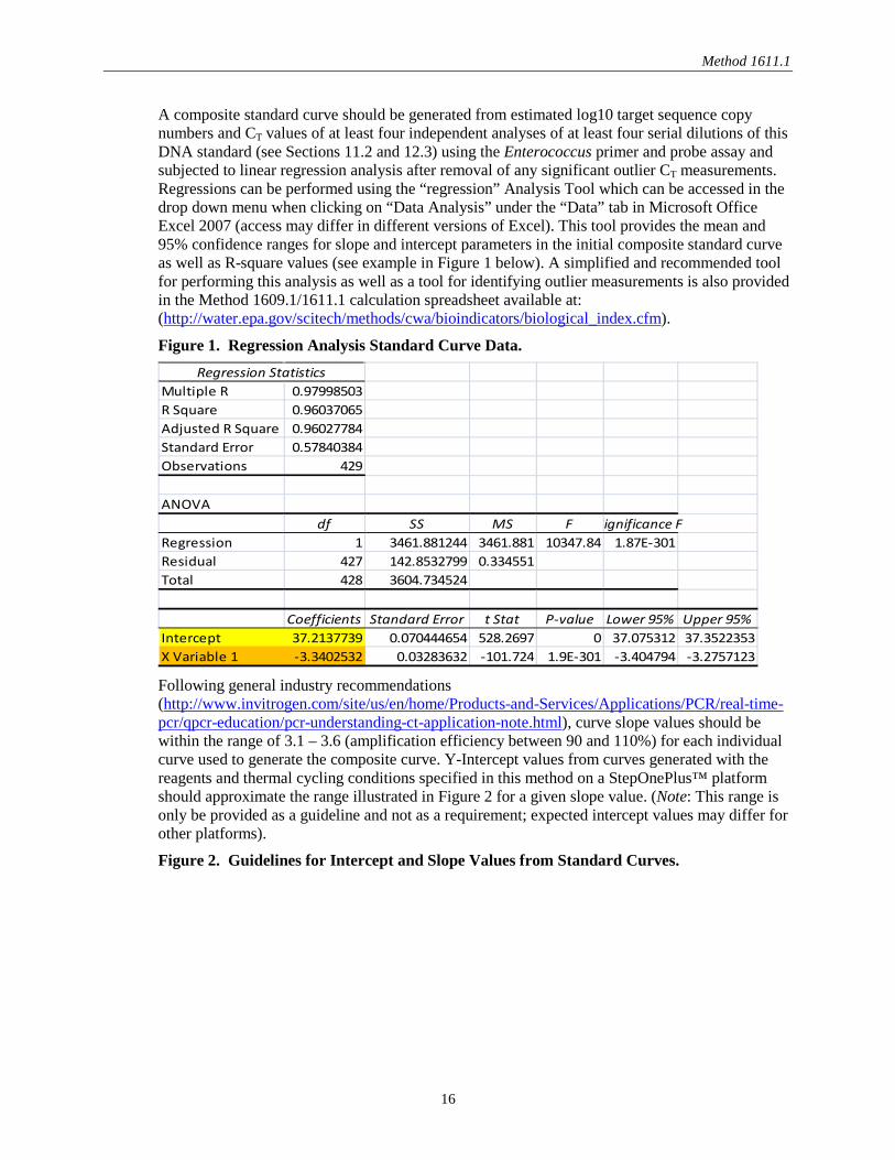
A composite standard curve should be generated from estimated log10 target sequence copy numbers and CT values of at least four independent analyses of at least four serial dilutions of this DNA standard (see Sections 11.2 and 12.3) using the Enterococcus primer and probe assay and subjected to linear regression analysis after removal of any significant outlier CT measurements. Regressions can be performed using the “regression” Analysis Tool which can be accessed in the drop down menu when clicking on “Data Analysis” under the “Data” tab in Microsoft Office Excel 2007 (access may differ in different versions of Excel). This tool provides the mean and 95% confidence ranges for slope and intercept parameters in the initial composite standard curve as well as R-square values (see example in Figure 1 below). A simplified and recommended tool for performing this analysis as well as a tool for identifying outlier measurements is also provided in the Method 1609.1/1611.1 calculation spreadsheet available at: (http://water.epa.gov/scitech/methods/cwa/bioindicators/biological_index.cfm).

Figure 1. Regression Analysis Standard Curve Data. Regression Statistics

Multiple R 0.97998503R Square 0.96037065Adjusted R Square 0.96027784Standard Error 0.57840384Observations 429

ANOVAdf SS MS F Significance F

Regression 1 3461.881244 3461.881 10347.84 1.87E-301Residual 427 142.8532799 0.334551Total 428 3604.734524

Coefficients Standard Error t Stat P-value Lower 95% Upper 95%Intercept 37.2137739 0.070444654 528.2697 0 37.075312 37.3522353X Variable 1 -3.3402532 0.03283632 -101.724 1.9E-301 -3.404794 -3.2757123 Following general industry recommendations (http://www.invitrogen.com/site/us/en/home/Products-and-Services/Applications/PCR/real-time-pcr/qpcr-education/pcr-understanding-ct-application-note.html), curve slope values should be within the range of 3.1 – 3.6 (amplification efficiency between 90 and 110%) for each individual curve used to generate the composite curve. Y-Intercept values from curves generated with the reagents and thermal cycling conditions specified in this method on a StepOnePlus™ platform should approximate the range illustrated in Figure 2 for a given slope value. (Note: This range is only be provided as a guideline and not as a requirement; expected intercept values may differ for other platforms).

Figure 2. Guidelines for Intercept and Slope Values from Standard Curves.

16

Method 1611.1

The R square values from regressions of these curves should ideally be 0.99 or greater. A convenient ANCOVA test for determining similarity of curves is provided in the Method 1609.1/1611.1 calculation spreadsheet. In the event that the combination of slope and intercept values or R square values from the regressions of one or more individual curves are substantially outside of the guidelines in Figure 2 or differ significantly from the other curves generated by the individual laboratory, these curves should be repeated. Amplification efficiency factor (AF) values can be calculated from the slope of the initial composite standard curve as described in Section 12.3.

From that point on, it is highly recommended that additional standard curves be generated from triplicate analyses of these same diluted standard samples with each new lot of TaqMan® master mix reagents or primers and probes to demonstrate comparable performance by the new reagents. The R square values from regressions of these curves should ideally be 0.99 or greater after removal of any outlier CT measurements. Comparable performance is assessed by the slopes of the new curves which should be within the range of values from the initial curves established by the individual laboratory. These assessments can be made either empirically or preferably by using the ANCOVA test in the Method 1609.1/1611.1 calculation spreadsheet.

In the event that the slope value from a subsequent standard curve regression is outside of the initial range, the standards should be re-analyzed. If this difference persists, new working stocks of the reagents should be prepared and the same procedure repeated. Failure to meet this criterion or the observation of a significantly higher intercept value also may be an indication of deterioration of the DNA standards. New serial dilutions can be prepared from a freezer stock of the DNA standard (see Section 11.2) or frozen aliquots of the previously prepared standards can be thawed and analyzed as described above. If the differences continue to persist, a new composite standard curve should be generated and the AF values recalculated as described above.

9.11 Calibrator samples — The cell concentration of each cultured E. faecalis stock suspension used for the preparation of calibrator sample extracts should be determined as described in Section 11.1. The manufacturer’s lot-specific certificate of analysis can be used to identify cell numbers in BioBalls. Initially, a minimum of four sets of calibrator sample extracts should be prepared

17

Method 1611.1

and analyzed on different days from different freezer-stored aliquots of these stocks or from different BioBalls (i.e., two or three (three is recommended) frozen cell or BioBall® extracts prepared per day and analyzed in duplicate on at least four different days) as described in Section 11.3 or 11.4. Dilutions of these calibrator sample extracts equivalent to the anticipated dilutions of the test samples used for analysis (e.g., 1, 5 and/or 25-fold) should be analyzed induplicate with different preparations of the Entero/IAC and Salmon DNA (Sketa 22) assay mixes (Section 11.8) on each day. The overall average and standard deviation of the Entero/IAC and Salmon DNA (Sketa 22) assay ΔCT values from these analyses should be determined for each relevant dilution after removal of any extreme measurements (> ± 3 standard deviations). A simple test for identifying extreme measurements is to exclude any measurements that are suspected of being extreme from the data set, determine the standard deviation of the remaining measurements and then determine whether the excluded measurements are within ± 3 standard deviations of the mean. The mean ΔCT value for each calibrator sample and the overall mean and standard deviation of these ΔCT values should also be calculated to obtain initial laboratory-specific baseline values. These calculations are automatically performed in the Method 1609.1/1611.1 calculation spreadsheet. From that point on, fresh calibrator sample extracts should be prepared from an additional frozen aliquot of the same stock cell suspension or from the same lot of BioBalls at least weekly either before or with preparation and analyses of each batch of test samples as described in Section 11.3 or 11.4. Dilutions of each new calibrator sample extract equivalent to the initial dilutions (e.g., 1, 5 and/or 25 fold) should be analyzed in duplicate using the Entero/IAC and Sketa22 assays. Each individual Entero and Sketa22 CT measurement and the mean ΔCT value from these analyses should be within ± 3 standard deviations from the laboratory’s mean baseline values from analyses of their initial calibrator sample extracts. Laboratories will be able to use ongoing calibrator sample results if at least one of the Entero and Sketa22 CT measurements meets this acceptance criterion. They may, however, wish to adopt more stringent QC requirements such as, for example, a majority or all of the CT measurements having to meet this criterion. If, as expected, more than one of the calibrator sample Entero and Sketa22 CT values meets this criterion, the average of the acceptable CT values from each assay should be taken and the average Sketa22 CT value should be subtracted from the average Entero CT value to give a mean ΔCT value. The mean ΔCT value also should meet the within 3 standard deviations criterion. Results from calibrator samples that do not meet the laboratory’s criteria should not be used for calculating test sample results. These analyses are automatically performed in the Method 1609.1/1611.1 calculation spreadsheet. If the calibrator sample measurements do not meet the laboratory’s acceptance criteria, new calibrator extracts should be prepared from another frozen aliquot of the same stock cell suspension or lot of BioBalls and analyzed in the same manner as described above. If the results are still not within the acceptance range, the reagents should be checked by the generation of a standard curve as described in Section 9.10. Calibrator samples prepared from new cultured E. faecalis cell suspensions or new lots of BioBalls must also meet the laboratory’s ongoing acceptance criterion. If these samples repeatedly fail the criteria, the above procedures for determining initial calibrator sample ΔCT measurements should be repeated with samples prepared from the new cultured E. faecalis cell suspension or lot of BioBalls. Note: The 25-fold dilution is not applicable with extracts of laboratory-prepared calibrator samples containing <1000 cells per sample or extracts of BioBall® calibrator samples, as these dilutions may contain target sequence quantities that are below the method’s limit of detection (see also Sections 9.14, 11.3 and/or 11.4).

9.12 Salmon DNA Sample Processing Control (SPC) sequence analyses — The Salmon DNA SPC is used as a DNA recovery control. Possibly due to difficulties in obtaining homogenous suspensions of this high molecular weight DNA or due to lot to lot variations in this product, some degree of variability in the CT values may be obtained from different initial preparations or

18

Method 1611.1

diluted batches of this DNA. Available data from the StepOnePlus™ platform suggest that CT values from undiluted 0.2 µg/mL salmon DNA extraction buffer s should fall within a range of ~ 18 – 22 units for this assay (values may differ for other platforms). Because it is not used as an absolute standard in the method, such variation may be acceptable, however, changes in CT values from new diluted batches of this DNA may necessitate the generation of new initial calibrator baseline ΔCT values in the Method 1609.1/1611.1 calculation spreadsheet for ongoing analyses (see Section 9.11). It is permissible to adjust the concentrations of new diluted batches of this DNA to obtain CT values that are similar to those of previous diluted batches in order to avoid having to generate new initial calibrator baseline ΔCT values.

While not mandatory, it is also good practice to prepare and analyze serial dilutions of the Salmon DNA extraction buffer as described for the Enterococcus DNA standards in Section 9.10. To our knowledge, rRNA gene operon copy numbers per genome have not been reported for the salmon species O. keta. However, log-transformed target sequence values of the Enterococcus DNA standards can be used for both assays for comparisons. A procedure is provided in a guidance document from the developers of the ΔΔCT calculation (Reference 16.1), for comparing the slopes of the Sketa22 and Enterococcus assays. (Note: serial dilutions of salmon and Enterococcus DNA do not necessarily need to be performed in the same tubes for this analysis as specified in the guidance document but it is recommended that the analyses of these dilutions be performed on the same plates). Available data indicates that the slopes of the Entero1A and Sketa22 assays meet the criterion for acceptable similarity specified in the guidance document. If results from an individual lab do not meet this criterion, it is recommended to make new working stocks of the Sketa22 assay probe and primers and/or new serial dilutions of the salmon DNA and repeat the test. In general, target DNA concentrations in test samples can be calculated as described in Section 12. However, the Salmon DNA PCR assay results for each test sample should be within 3 CT units of the mean of the similarly diluted calibrator Salmon DNA sample results. Higher CT values may indicate significant PCR inhibition or poor DNA recovery possibly due to physical, chemical, or enzymatic degradation. While poor DNA recovery is compensated for by the calculation method, a salmon DNA assay offset CT value of greater than 3 CT units suggests that total DNA recovery was < ~10% and therefore potentially unacceptably high levels of enterococci may not be detectable due to the very low recovery. When the Salmon PCR assay CT value is within the 3 CT unit cutoff, the result from the optional IAC assay can be used to further determine the acceptability of the sample result as indicated in Section 9.13 if this assay is used. Note: If salmon DNA assay CT values from analyses of a particular batch of test samples are all substantially higher or lower (e.g., > ±1 CT unit) than the mean of corresponding diluted calibrators samples, and this phenomenon is not normally observed for samples from this site, it is recommended that new calibrator samples be prepared and the test samples and new calibrator sample be re-analyzed. While consistent salmon DNA assay CT offsets between the test samples and calibrator samples of > 1 CT unit may be attributable to certain water matrices (Reference 16.4), such results have also been observed to be occasionally attributable to an as yet unidentified source of error in the analytical method. Therefore the validity of these types of salmon DNA assay results should be confirmed. Determination of percent recovery of matrix spikes of these test samples (see Section 9.5) also may be useful in determining whether the abnormal differences between salmon DNA assay CT values for these test samples and the calibrators are an artifact of the analytical method or represent true test sample effects on DNA recovery. Potential mitigation procedures involving the use of higher salmon DNA concentrations in the extraction buffer for extraction of samples from sites that consistently produces substantially higher CT measurements than those of corresponding diluted calibrators samples

19

Method 1611.1

have been proposed (Reference 16.4). Salmon DNA concentrations in the extraction buffer used to extract calibrator samples should always be equivalent to those used to extract test samples.

9.13 Internal Amplification Control (IAC) sequence analyses — The IAC assay is expected (and thus far has been demonstrated, Reference 16.4) to be a sensitive indicator of inhibition of the Enterococcus assay since the two assays utilize the same primer set and because the IAC template is added just prior to the reaction. A more stringent acceptance criterion has been adopted for this assay where test sample CT values cannot be offset by >1.5 units compared to negative control samples with no target DNA (Reference 16.4). The Enterococcus, IAC and salmon DNA PCR assays can be repeated on any samples that fail this criterion using a 5-fold higher dilution of the sample extracts. If the IAC assay CT value is now within the 1.5 CT unit acceptance range, the corresponding Enterococcus and salmon assay results from this dilution can now be accepted and used in the comparative CT calculation method (see Section 12) with Enterococcus and salmon assay CT results from equally diluted calibrator samples. As described in Section 7.23.3, mean CT values for calibrator and/or control samples with this assay are considered to be acceptable within a range of ~30-34 units for StepOnePlus™ platforms (values may vary for other platforms). These values have been found to be indicative of a sufficient quantity of IAC template for the assay to show acceptable reproducibility in measurements while not causing competitive inhibition of Enterococcus target sequence amplification. Note: In samples with very high concentrations of Enterococcus target sequences (e.g., > 105 – 106 copies/sample or > 103 – 104 copies/reaction), the IAC assay may fail the 1.5 CT offset criterion due to competitive inhibition by the Enterococcus target sequences. Available data indicate that Enterococcus sequence concentrations that are high enough to have this completive inhibitory effect on the IAC CT value will indicate unacceptable water quality so the IAC result can be ignored from the standpoint of beach advisory decisions with no further analysis required. For such samples however, it may be desirable to either add a higher quantity of IAC templates to the reaction or further dilute the sample extract to the point where the IAC result passes the 1.5 CT offset criterion in order to exclude the possibility of partial inhibition by the sample matrix. If a higher IAC template concentration is used in this repeat analysis and passes the 1.5 CT offset criterion, the Enterococcus assay CT value from the initial analysis should be used for calculating Enterococci densities in the test sample. If the sample extract is diluted, the Enterococcus assay CT value from the repeat analysis should be used in conjunction with CT results from equally diluted calibrator sample extracts for calculating Enterococci densities in the test sample as indicated above. Note: Use of the multiplex IAC assay is optional in this method but is highly recommended as a convenient surrogate test for identifying potential sample matrix inhibition and as a general positive control for each sample analysis. Determination of percent recovery of matrix spikes (see Section 9.5) is recommended to confirm the effects of problematic sample matrices on method performance.

9.14 Method Limit of Detection/Quantification — A report on the limit of quantification of the method is available at: http://water.epa.gov/scitech/methods/cwa/bioindicators/biological_index.cfm. The 33% coefficient of variation values in this report are acceptable. The reported values are for 5x-diluted extracts and can be extrapolated to undiluted and 25x-diluted extracts by dividing or multiplying by 5, respectively. These values can be used for determining acceptable NTC and method blank results (see Sections 9.7 and 9.8). Limits of detection will be considered as equivalent to these values for the purposes of documenting laboratory capability. Laboratories are encouraged to document a similar limit of detection capability as described in Section 11.2.23.5. Ability to detect a 5 target sequence copy/reaction sample as described in this section will provide this

20

Method 1611.1

documentation. Ability to detect a 10 target sequence copy/reaction standard as described in Section 11.2.25 will be considered as adequate.

10.0 Calibration and Standardization of Method-Related Instruments 10.1 Check temperatures in incubators twice daily with a minimum of 4 hours between each reading to

ensure operation within stated limits.

10.2 Check thermometers at least annually against a National Institute of Standards and Technology (NIST) certified thermometer or one that meets the requirements of NIST Monograph SP 250-23. Check columns for breaks.

10.3 Spectrophotometer should be calibrated each day of use using OD calibration standards between 0.01 - 0.5. Follow manufacturer instructions for calibration.

10.4 Micropipettors should be calibrated at least annually and tested for accuracy on a weekly basis. Follow manufacturer instructions for calibration.

10.5 Follow manufacturer instructions for calibration of real-time PCR instruments.

11.0 Procedure

Note: Procedures described in Section 11.1 can be omitted if laboratories choose to use commercially available E. faecalis cells (BioBalls) and procedures described in Section 11.2 can be omitted if laboratories choose to use DNA standards provided by EPA (see Appendix E). Preparation of calibrator, reference (PBS) matrix spike and matrix spike samples with BioBalls is described in Section 11.4. Preparation and use of EPA plasmid DNA standards is described in Section 11.5. Laboratory-prepared E. faecalis cell suspensions (Section 11.1), DNA standards (Section 11.2) and preliminary calibrator samples (Section 11.3) should be prepared and analyzed in advance of any test sample analyses (see Sections 9.10 and 9.11).

11.1 Preparation of laboratory-cultured E. faecalis cell suspensions for DNA standards, calibrator samples, matrix spike samples and spiked reference (PBS) matrix filters

11.1.1 Thaw an E. faecalis (ATCC® 29212™) stock culture (Section 7.8) and streak for isolation on BHIA plates. Incubate plates at 37°C ± 0.5°C for 24 ± 2 hours.

11.1.2 Pick an isolated colony of E. faecalis from BHIA plates and suspend in 1 mL of sterile PBS and vortex.

11.1.3 Use 10 μL of the 1 mL suspension of E. faecalis to inoculate a 10 mL BHIB tube. Place the inoculated tube and one uninoculated tube (sterility check) on a shaker set at 250 rpm [revolutions per minute] and incubate at 37°C ± 0.5°C for 24 ± 2 hours. Note: It is advisable to verify that the selected colony is Enterococcus as described, for example, in Section 12.0 of EPA Method 1600.

11.1.4 After incubation, centrifuge the BHIB containing E. faecalis for 5 minutes at 6000 × g.

11.1.5 Aspirate the supernatant and resuspend the cell pellet in 10 mL PBS.

21

Method 1611.1

11.1.6 Repeat the two previous steps twice and suspend final E. faecalis pellet in 5 mL of sterile PBS. Label the tube as E. faecalis undiluted stock cell suspension, noting cell concentration after determination by the following steps.

11.1.7 Determination of calibrator sample cell concentrations based on the plating method below.

Note: BHIA plates should be prepared in advance if this option is chosen. For enumeration of the E. faecalis undiluted cell suspension, dilute and inoculate according to the following.

A) Mix the E. faecalis undiluted cell suspension by vigorously shaking the 5 mL tube a minimum of 25 times. Use a sterile pipette to transfer 0.5 mL of the undiluted cell suspension to 49.5 mL of sterile PBS, cap, and mix by vigorously shaking the tube a minimum of 25 times. With care, a 50 mL tube may be used. This is cell suspension dilution “A”. A 1.0 mL volume of dilution “A” is 10-2 mL of the original undiluted cell suspension.

B) Use a sterile pipette to transfer 5.0 mL of cell suspension dilution “A” to 45 mL of sterile PBS, cap, and mix by vigorously shaking the tube a minimum of 25 times. This is cell suspension dilution “B”. A 1.0 mL volume of dilution “B” is 10-3 mL of the original undiluted cell suspension.

C) Use a sterile pipette to transfer 5.0 mL of cell suspension dilution “B” to45 mL of sterile PBS, cap, and mix by vigorously shaking the tube a minimum of 25 times. This is cell suspension dilution “C”. A 1.0 mL volume of dilution “C” is 10-4 mL of the original undiluted cell suspension.

D) Use a sterile pipette to transfer 5.0 mL of cell suspension dilution “C” to 45 mL of sterile PBS, cap, and mix by vigorously shaking the tube a minimum of 25 times. This is cell suspension dilution “D”. A 1.0 mL volume of dilution “D” is 10-5 mL of the original undiluted cell suspension.

E) Use a sterile pipette to transfer 5.0 mL of cell suspension dilution “D” to 45 mL of sterile PBS, cap, and mix by vigorously shaking the tube a minimum of 25 times. This is cell suspension dilution “E”. A 1.0 mL volume of dilution “E” is 10-6 mL of the original undiluted cell suspension.

F) Prepare BHIA (Section 7.6). Ensure that agar surface is dry. Note: To ensure that the agar surface is dry prior to use, plates should be made several days in advance and stored inverted at room temperature or dried using a laminar-flow hood.

G) Each of the following will be conducted in triplicate, resulting in the evaluation of nine spread plates: • Pipet 0.1 mL of dilution “C” onto surface of BHIA plate [10-5 mL (0.00001)

of the original cell suspension]. • Pipet 0.1 mL of dilution “D” onto surface of BHIA plate [10-6 mL (0.000001)

of the original cell suspension]. • Pipet 0.1 mL of dilution “E” onto surface of BHIA plate [10-7 mL

(0.0000001) of the original cell suspension]. H) For each spread plate, use a sterile bent glass rod or spreader to distribute

inoculum over surface of medium by rotating the dish by hand or on a rotating turntable.

22

Method 1611.1

I) Allow inoculum to absorb into the medium completely.

J) Invert plates and incubate at 35°C ± 0.5°C for 24 ± 4 hours. K) Count and record number of colonies per plate. Refer to the equation below for

calculation of undiluted cell suspension concentration.

CFU/mLundiluted = CFU1 + CFU2 +.....+ CFUn

V1 + V2 + ... + Vn

Where:

CFU/mLundiluted = E. faecalis CFU [colony forming units]/mL in undiluted cell suspension

CFU = number of colony forming units from BHIA plates yielding counts within the ideal range of 30 to 300 CFU per plate

V = volume of undiluted sample in each BHIA plate yielding counts within the ideal range of 30 to 300 CFU per plate

n = number of plates with counts within the ideal range Table 7. Example Calculations of E. faecalis Undiluted Cell Suspension Concentration

Examples CFU / plate (triplicate analyses) from BHIA plates E. faecalis CFU / mL in undiluted

suspensiona 10-5 mL plates 10-6 mL plates 10-7 mL plates

Example 1 275, 250, 301 30, 10, 5 0, 0, 0 (275+250+30) / (10-5+10-5+10-6) = 555 / (2.1 × 10-5) = 26,428,571 =

2.6 × 107 CFU / mL

Example 2 TNTCb, TNTC, TNTC TNTC, 299, TNTC 12, 109, 32 (299+109+32) / (10-6+10-7+10-7) = 440 / (1.2 × 10-6) = 366,666,667 =

3.7 × 108 CFU / mL a Cell concentration is calculated using all plates yielding counts within the ideal range of 30 to 300 CFU per plate b Too numerous to count

11.1.8 Transfer aliquots of the remaining cell suspension into sterile tubes. Aliquot volumes should be based on the concentration estimate of the cell suspension determined in Section 11.7. Aliquots for DNA standard preparations (Section 11.2) should contain an estimated total of ~109 CFU and aliquots for preparation of sub-stocks for calibrator and matrix spike samples (see paragraph below) should contain ~108 CFU. So for example, if the estimated concentration of the cell suspension is 109 CFU/mL, transfer 1 mL aliquots for DNA standard preparations and 0.1 mL aliquots for sub-stocks. Note: If the concentration estimate of the cell suspension, determined in Section 11.7, is greater than 109 CFU/mL, it is recommended to dilute either part or all of this cell suspension to approximately this concentration or lower before proceeding with making the aliquots. This is so that the 108 CFU aliquot volumes will be no less than 0.1 mL. Prepare as many aliquots of each as needed and either freeze or discard the remainder of the cell suspension. Freeze each of the aliquot tubes at -80°C except one tube containing ~108 CFU. Note: Cell suspension should be stirred or gently vortexed repeatedly while aliquoting. To make substocks for calibrator and matrix spike samples (Section 11.3), transfer the entire contents of the unfrozen tube containing ~108 CFU of E. faecalis stock cell suspension to a sterile tube or bottle containing ~100 mL of PBS buffer (100 mL minus the volume of the cell suspension) to make a cell suspension containing ~106 CFU/mL (108 CFU in a final volume of 100 mL). Transfer as many 0.2 ml aliquots of this

23

Method 1611.1

suspension as needed to sterile tubes (making sure to gently vortex or shake the tube or bottle repeatedly while aliquoting) and freeze the substock aliquots at -80°C. Note: Frozen aliquots of the original stock suspension may be thawed one time each to make additional substocks for calibrator and matrix spike samples as described above.

11.2 Preparation of E. faecalis genomic DNA standards

11.2.1 Remove one tube containing ~109 CFU of E. faecalis cells (Section 11.1.8) from freezer and thaw completely.

11.2.2 Pellet the cells by centrifugation at 12,000 × g for one minute, draw off and discard supernatant and resuspend the cell pellet in a final volume of 1 mL AE buffer.

11.2.3 Transfer 0.5 mL aliquots of the cell suspension to two extraction tubes with glass beads. Tightly close the tubes, making sure that the O-rings are seated properly.

11.2.4 Place the tubes in bead beater and shake for 60 seconds at the maximum rate (5000 rpm).

11.2.5 Remove the tubes from the mini bead beater and centrifuge at 12,000 × g for one minute to pellet the glass beads and debris.

11.2.6 Using a 200 μL micropipettor, transfer 350 μL of supernatants to sterile 1.7 mL microcentrifuge tubes. Recover supernatants without disrupting the glass beads at the tube bottom.

11.2.7 Centrifuge crude supernatants at 12,000 × g for 5 minutes and transfer 300 μL of clarified supernatant to clean, labeled 1.7 mL low retention microcentrifuge tubes, taking care not to disturb the pellet.

11.2.8 Add 1 μL of 5 μg/μL RNase A solution to each clarified supernatant, mix by vortexing and incubate at 37°C for 1 hour. Note: Steps 11.2.9 − 11.2.15 may be substituted with an optional method if a DNA purification procedure is chosen other than the DNA-EZ purification kit. In such a case, manufacturer instructions should be followed rather than these steps, and the method should be followed beginning at step 11.2.16.

11.2.9 Add 0.6 mL of binding buffer solution from a DNA-EZ purification kit to each of the RNase A-treated extracts and mix by vortexing. Note: In general, a minimum concentration of 5 × 108 cells is required for this step.

11.2.10 If using the DNA-EZ purification kit, perform the following steps. Insert one DNAsure™ column from the DNA-EZ purification kit into a collection tube (also provided with kit) for each of the two extracts. Transfer the extract and binding buffer mixtures from Section 11.2.9 to a DNAsure™ column and collection tube assembly and centrifuge for 1 minute at 12,000 × g.

11.2.11 Transfer each of the DNAsure™ columns to new collection tubes. Discard previous collection tubes and collected liquid.

11.2.12 Add 500 μL EZ-Wash Buffer from the DNA-EZ purification kit to each of the DNAsure™ columns and centrifuge at 12,000 × g for 1 minute. Discard the liquid in the collection tube.

11.2.13 Repeat step 11.2.12. 11.2.14 Transfer each of the DNAsure™ columns to a clean, labeled 1.7 mL low retention

microcentrifuge tube and add 50 μL of DNA elution buffer to each column. Centrifuge

24

Method 1611.1

for 30 seconds at 12,000 × g. Repeat this procedure again to obtain a total DNA eluate volume of ~100 μL from each column.

11.2.15 Pool the two eluates to make a total volume of approximately 200 μL. 11.2.16 Transfer entire purified DNA eluate volume from each column to a clean and sterile

microcuvette for UV spectrophotometer and read absorbance at 260 and 280 nm. (Note: The cuvette should be blanked with DNA elution buffer before reading the sample). If necessary, the sample may be diluted with elution buffer to reach minimum volume that can be accurately read by the spectrophotometer (see manufacturer’s recommendation); however, this may reduce the DNA concentration to a level that cannot be accurately read by the spectrophotometer. If available, readings can be taken of 2 μL aliquots of the sample with a NanoDrop™ Spectrophotometer.

11.2.17 The sample is acceptable as a standard if ratio of OD260/OD280 readings is > to 1.75. 11.2.18 Record UV spectrophotometer results.

11.2.19 Calculate total DNA concentration in sample by formula:

OD260 reading × 50 ng/μL DNA/OD260 11.2.20 Transfer sample back to labeled 1.7 mL non-retentive microcentrifuge tube and store at

-20°C. 11.2.21 Using total DNA concentration (Section 11.2.19), calculate E. faecalis PCR target

sequence concentration (TSC) in purified extract (Section 9.10). Example:

OD260 = 0.7271 Total DNA concentration = OD260 Reading × 50 ng/µL

0.7271 × 50 = 36.36 ng/µL = 36.36 × 106 fg/µL = 3.636 × 107 fg/µL 3.636 × 107 fg/µL × 4 lsrRNA gene copies = 4.04 × 107 gene copies/µL 3.6 fg/genome genome

11.2.22 Record UV spectrophotometer results and all calculations.

11.2.23 In appropriately labeled 1.7 mL low retention microcentrifuge tubes, perform serial dilutions using AE buffer to prepare DNA standards of 4 × 104/5 μL, 4 × 103 TSC/5 μL, 4 × 102 TSC/5 μL, 40 TSC/5 μL, and 10 TSC/5 μL (see below).

Note: Perform initial dilution of purified and quantified DNA as required to achieve a stock concentration of 2 × 108 TSC/5 μL4 × 107 TSC/5 μL with AE buffer prior to initiating serial dilutions. For the example concentration of 4.04 × 107 TSC/μL (2.02 × 108 TSC/5 μL) shown in Section 11.2.21, this would be a 5.05-fold dilution (e.g., 1 mL: 4.05 mL). It is recommended that DNA stocks (i.e., > 4 × 104 TSC/5 μL) be stored and manipulated in a different room than that used for routine sample processing in order to minimize the potential for laboratory contamination. 11.2.23.1 Perform 10-fold serial dilutions of the 4 × 107 TSC/5 μL stock (e.g.,100

μL : 900 μL) with AE buffer to achieve stocks of 4 × 106 TSC/5 μL; and 4 × 105 TSC/5 μL.

11.2.23.2 Perform 10-fold dilution of 4 × 105 TSC /5 μL stock (e.g., 100 μL : 900 μL) with AE buffer to achieve the first standard: 4 × 104 TSC/5 μL.

11.2.23.3 Perform successive 10-fold serial dilutions of the 4 × 104 TSC/5 μL standard (e.g., 100 μL : 900 μL) to achieve 4 × 103 TSC/5 μL; 4 × 102 TSC/5 μL and 40 TSC/5 μL standards.

25

Method 1611.1

11.2.23.4 Perform a 4-fold dilution of 40 TSC/5 μL standard (e.g., 100 μL : 300 μL) to achieve 10 TSC/5 μL standard.

11.2.23.5 (Optional) Perform a final 2-fold dilution of 10 TSC/5 μL standard (e.g., 25 μL : 25 μL) to achieve 5 TSC/5 μL. Note: Preparation and analysis of this dilution is not necessary for determining standard curves but is recommended for determining limit of detection capability (see Section 9.14). CT values resulting from true positive logarithmic amplification traces should be obtained from at least 90% of the analyses of this dilution to document the laboratory’s limit of detection capability with the method. Note: It is also strongly recommended that further dilutions of the 5 TSC/5 μL dilution be analyzed to obtain most probable number estimates of target sequence concentration as described in Reference 16.6 (a detailed protocol is provided in Appendix D) when using laboratory prepared standards. Mean target sequence estimates in the standards, as determined by this technique, should be consistent with the spectrophotometric based estimates. If they are not, the use of DNA standards that have been prepared and tested by the EPA is recommended. This analysis should not be necessary when using these DNA standards (see Section 11.5).

11.2.24 Store DNA standards in refrigerator at 4°C. For long term storage, freeze aliquots at -80°C.

11.2.25 Generate DNA standard curves by analyzing 5 μL aliquots of the 40,000, 4000, 400, 40 and 10 TSC/5 μL standards with 3 replicate analyses of each standard per curve according to Section 11.9 (AB) or 11.10 (Smart Cycler®), as appropriate. (Note: EPA recommends the generation of at least four independent standard curves (from separate instrument runs performed on different days and/or with different mixes of reagents) for determination of a composite standard curve as detailed in Section 9.10. It is further recommended that initial analyses of calibrator sample extracts, as detailed in Section 9.11, be performed at the same time (preferably in the same instrument runs if using 96 well format instruments) as the analyses of these standards). Note: CT values resulting from true positive logarithmic amplification traces should be obtained from at least 95% of the analyses of each standard to document each laboratory’s limit of detection capability with the method.

11.3 Preparation and DNA extraction of E. faecalis calibrator, matrix spike and reference (PBS) matrix spike samples prepared from laboratory-grown cell suspensions. Note: If using BioBalls to prepare calibrator, matrix spike and reference (PBS) matrix spike samples see Section 11.4.

11.3.1 Either two or three calibrator sample extracts should be prepared and extracted either daily or at least weekly during water sample analyses. Calibrator samples can be prepared and extracted either in advance of, or in parallel with water sample filters.

11.3.2 Remove one tube containing a 0.2 mL aliquot of E. faecalis substock cell suspension (Section 11.1.8) from the freezer and allow to thaw. Dilute the cell suspension 100-fold with PBS buffer (e.g., dilute the 0.2 mL aliquot with 0.8 ml of PBS buffer and then transfer this entire 1 mL suspension to a larger tube containing 19 mL PBS) and mix thoroughly by vortexing. Note: This dilution should produce an estimated concentration of ~104 CFU/mL (see section 11.8).

11.3.3 Prepare one membrane filtration system with polycarbonate filter as described in Sections 11.6.1 – 11.6.2 for each calibrator sample to be prepared (see Section 11.3.1).

26

Method 1611.1

11.3.4 Filter 1 mL aliquots of the diluted cell suspension from step 11.3.2 (calibrator samples) through each membrane filtration system prepared in step 11.3.3. After filtering, wash each membrane with 20 mL of sterile PBS (Section 7.4) and continue filtration until all liquid has been pulled through the filter. Turn off the vacuum and remove the funnel from the filter base.

11.3.5 Label extraction tubes with glass beads (Section 7.18) to identify samples. Leaving the filters on the filtration unit base, fold the filter into a cylinder with the sample side facing inward, being careful to handle the filters only on the edges, where the filters have not been exposed to the sample. Insert each folded filter into a labeled extraction tube with glass beads.

11.3.6 Dispense 600 μL of Salmon DNA/extraction buffer (Section 7.12) into each extraction tube with glass beads and filter.

11.3.7 Place the tubes with filters in the bead beater and shake for 60 seconds at the maximum rate (5000 rpm).

11.3.8 Remove the tubes from the bead beater and centrifuge at 12,000 × g for one minute to pellet the glass beads and debris.

11.3.9 Using a 200 μL micropipettor, transfer the crude supernatant to the corresponding labeled sterile 1.7 mL microcentrifuge tube. Transfer 400 μL of supernatant taking care to minimize picking up glass beads at the tube bottom. Note: The filter will normally remain intact during the bead beating and centrifugation process. Generally, 400 μL of supernatant can be easily collected.

11.3.10 Centrifuge at 12,000 × g for 5 minutes and transfer ~350 μL of clarified supernatant to a clean, labeled 1.7 mL tube, taking care not to disturb the pellet. Note: Cell pellet may not be visible in calibrator samples.

11.3.11 Label the tubes as undiluted or 1x E. faecalis calibrator extracts. Label additional 1.7 mL tubes for 5 (and 25) fold dilutions (if necessary). In appropriately labeled tubes, using a micropipettor, add a 50 μL aliquot of each 1x E. faecalis calibrator extracts and dilute each with 200 μL AE buffer (Section 7.11) to make 5 fold dilutions. In appropriately labeled tubes using a micropipettor, add a 50 μL aliquot of each 5 fold dilution and dilute each with 200 μL AE buffer to make 25 fold dilutions if necessary.

11.3.12 Refrigerate the extracts until ready to analyze. Calibrator extracts can be held in this manner and reused for repeated analyses with different batches of water sample extracts for up to 1 week.

11.3.13 Matrix spike samples:

11.3.13.1 Prepare matrix spike samples for interference testing at frequencies

indicated in Section 9.5. Samples should be spiked with the same diluted E. faecalis cell suspensions as used for preparing daily or weekly calibrator samples. Diluted E. faecalis cell suspensions can be held in refrigerator for up to one week for the latter purpose.

11.3.13.2 Transfer a 1 mL aliquot of the diluted cell suspension from Section 11.3.2 to 100 mL (or 50 mL – see Section 11.6.4) of the water sample selected for testing to create the matrix spike sample.

27

Method 1611.1

11.3.13.3 Filter spiked water sample as described in Section 11.6 (see guidance in Section 9.5 concerning pairing of spiked and unspiked water sample filters for interference testing).

11.3.13.4 Transfer each filter to labeled extraction tube with glass beads and 600 μL of Salmon DNA/extraction buffer.

11.3.13.5 Extract matrix spike and corresponding unspiked water sample filters in same manner as described for calibrator samples in Sections 11.3.9 – 11.3.14. Analyze matrix spike and unspiked water sample and calibrator sample extracts in parallel if possible (as described in Sections 11.8 and 11.9 or 11.10) the same day the water sample extracts are prepared.

11.3.14 Reference (PBS) matrix spike samples: 11.3.14.1 Prepare reference (PBS) matrix spike samples at frequencies described in

Sections 9.3 or 9.4. Samples should be spiked with the same cell suspensions as used for preparing daily or weekly calibrator samples.

11.3.14.2 Prepare membrane filtration system with polycarbonate filter(s) as described in Sections 11.6.1 – 11.6.2.

11.3.14.3 Transfer a 1 mL aliquot of the diluted cell suspension from Section 11.3.2 to 50 or 100 mL of PBS to create the reference (PBS) matrix spike sample.

11.3.14.4 Filter reference (PBS) matrix spike sample as described in Section 11.6. 11.3.14.5 Transfer each filter to labeled extraction tube with glass beads and 600 μL

of Salmon DNA/extraction buffer. 11.3.14.6 Analyze reference (PBS) matrix spike and calibrator sample extracts in

parallel if possible (as described in Sections 11.8 and 11.9 or 11.10) within one week of their preparation.

11.4 Preparation and DNA extraction of E. faecalis calibrator, matrix spike and reference (PBS) matrix spike samples from BioBalls

11.4.1 Either two or three calibrator extracts should be prepared and extracted either daily or at least weekly during water sample analyses. BioBall® calibrator samples can be prepared and extracted either in advance of, or in parallel with water sample filters. Note: Upon receipt, BioBalls should be stored at -20°C. Culturing of BioBalls prior to spiking is not necessary, as they can be spiked directly into a sample once the vial is opened.

11.4.2 Open one BioBall® vial for each calibrator sample to be prepared. Aseptically add each E. faecalis BioBall® to 1 mL of PBS and dissolve by gentle vortexing. Note: Each BioBall® contains ~550 CFU of E. faecalis. See manufacturer’s lot-specific certificate of analysis to identify exact cell (i.e., CFU) numbers.

11.4.3 Prepare one membrane filtration system with polycarbonate filter as described in Sections 11.6.1 – 11.6.2 for each calibrator sample.

11.4.4 Filter each BioBall® cell suspension (calibrator sample) through a membrane filtration system with a polycarbonate filter. After filtering, wash each membrane with 20 mL of sterile PBS (Section 7.4) and continue filtration until all liquid has been pulled through the filter. Turn off the vacuum and remove the funnel from the filter base.

28

Method 1611.1

11.4.5 Label extraction tubes with glass beads (Section 7.18) to identify samples. Leaving the filter on the filtration unit base, fold into a cylinder with the sample side facing inward, being careful to handle the filter only on the edges, where the filter has not been exposed to the sample. Insert the folded filter into the labeled extraction tube with glass beads. Prepare one filter for each BioBall® sample filtered in this manner.

11.4.6 Dispense 600 μL of Salmon DNA/extraction buffer (Section 7.12) into each extraction tube with glass beads and filter.

11.4.7 Tightly close the tubes, making sure that the O-ring is seated properly.

11.4.8 Extract BioBall® calibrator sample filters in same manner as described for laboratory-prepared calibrator samples in Sections 11.3.9 – 11.3.14.

11.4.9 Label the tubes as undiluted or 1x E. faecalis calibrator extracts. Label additional 1.7 mL tubes for 5 fold dilutions. In appropriately labeled tubes, using a micropipettor, add a 50 μL aliquot of each 1x E. faecalis BioBall® calibrator extracts and dilute each with 200 μL AE buffer (Section 7.11) to make 5 fold dilutions.

11.4.10 Refrigerate the extracts until ready to analyze. BioBall® calibrator extracts can be held in this manner and reused for repeated analyses with different batches of water sample extracts for up to 1 week.

11.4.11 Matrix spike samples: 11.4.11.1 Prepare matrix spike samples for interference testing at frequencies

indicated in Section 9.5. Samples should be spiked with the same lot of BioBalls as used for preparing daily or weekly calibrator samples.

11.4.11.2 Prepare membrane filtration system with polycarbonate filter(s) as described in Sections 11.6.1 – 11.6.2.

11.4.11.3 Aseptically transfer one BioBall® to 100 mL (or 50 mL – see Section 11.6.4) of the water sample selected for testing as described in Section 11.4.2 and allow to dissolve to create the matrix spike sample.

11.4.11.4 Filter matrix spike sample as described in Section 11.6 (see guidance in Section 9.5 concerning pairing of matrix spike and unspiked water sample filters for interference testing)

11.4.11.5 Transfer each filter to extraction tube with glass beads and 600 μL of Salmon DNA/extraction buffer.

11.4.11.6 Extract matrix spike and corresponding unspiked water sample filters in same manner as described for calibrator samples in Sections 11.3.9 – 11.3.14. Analyze spiked and unspiked water sample and calibrator sample extracts in parallel if possible (as described in Sections 11.8 and 11.9 or 11.10) the same day the water sample extracts are prepared.

11.4.12 Reference (PBS) matrix spike samples: 11.4.12.1 Prepare reference (PBS) matrix spike samples at frequencies described in

Section 9.4. Samples should be spiked with the same lot of BioBalls as used for preparing daily or weekly calibrator samples.

11.4.12.2 Prepare membrane filtration system with polycarbonate filter(s) as described in Sections 11.6.1 – 11.6.2.

29

Method 1611.1

11.4.12.3 Aseptically transfer one BioBall® to 50 or 100 mL of PBS as described in Section 11.4.2 and allow to dissolve to create reference (PBS) matrix spike sample.

11.4.12.4 Filter spiked PBS reference (PBS) matrix sample as described in Section 11.6.

11.4.12.5 Transfer each filter to extraction tube with glass beads and 600 μL of Salmon DNA/extraction buffer and label.

11.4.12.6 Extract reference (PBS) matrix spike sample filters in same manner as described for calibrator samples in Sections 11.3.9 – 11.3.14. Analyze reference (PBS) matrix spike and calibrator sample extracts in parallel if possible (as described in Sections 11.8 and 11.9 or 11.10) within one week of their preparation.

11.5 Use of EPA plasmid DNA standards (see Appendix E for instructions on acquiring these standards). 11.5.1 DNA standards will be provided as a kit/package consisting of 5 components: Dilution 1:

~4×104 copies/5 μL; Dilution 2: ~4×103 copies/5 μL; Dilution 3: ~4×102 copies/5 μL; Dilution 4: ~4×101 copies/5 μL; Dilution 5: ~1×101 copies/5 μL. Note: Mean concentration estimates and standard deviations may vary slightly by lot. Lot-specific concentration information will be provided with each kit.

11.5.2 Upon receipt of the kit, freeze all components at -80°C until ready to use (Note: if -80°C storage capability is not available, it is recommended that the kit be stored at -20°C and used as soon as possible as described below).

11.5.3 Thaw kit components and store at 4°C. 11.5.4 Generate DNA standard curves by analyzing 5 μL aliquots of kit components 1-5 with 3

replicate analyses of each component per instrument run according to Section 11.9 (Life Technologies/AB) or 11.10 (Smart Cycler®), as appropriate. Note: Sufficient volumes of components 1-5 are provided in each kit to generate at least twelve standard curves in this manner. EPA recommends the generation of at least four independent standard curves (from separate instrument runs performed on different days and/or with different mixes of reagents) for determination of a composite standard curve as detailed in Section 9.10. EPA further recommends that these analyses be completed within one month of thawing the kit components. Finally, it is recommended that initial analyses of at least eight independent calibrator sample extracts, as detailed in Section 9.11, be performed at the same time (preferably in the same instrument runs if using 96 well format instruments) as the analyses of these standards. Aliquots of the kit components that are not used for initial analysis after initial thawing immediately should be transferred to low retention tubes (see Section 6.24) and re-frozen one time at -80°C for subsequent use. Repeated freezing and thawing of these components should be avoided.

11.6 Water sample filtration

Note: It is required that at least one water sample filtration blank (method blank) be prepared for every PCR run (Section 9.8) and analyzed by the same procedure as the water samples. 11.6.1 Assemble manifold (Section 6.11), safety trap (Section 6.12) and vacuum system

(Section 6.9) and connect membrane filtration unit(s) (Section 6.8) to manifold. 11.6.2 Place a polycarbonate filter (Section 6.14) on each filter base, and attach the funnel to the

base so that the membrane filter is now held between the funnel and the base. Note: Most

30

Method 1611.1

disposable plastic membrane filtration units (e.g., Nalgene CN 130-4045,CN 145-0045, or equivalent) are provided with a cellulose nitrate filter that must be removed and replaced with the polycarbonate filter, do not remove filter support pad provided with the unit.

11.6.3 Shake the sample bottle vigorously 25 times to distribute the bacteria uniformly, and measure 100 mL of sample (or 50 mL – see Section 11.6.4) into the funnel. (Note: Use of the graduations in most brands of disposable plastic membrane filtration units is acceptable for measuring)

11.6.4 Filter 100 mL of water sample. After filtering the sample, rinse the sides of the funnel with 20 mL of sterile PBS (Section 7.4) and continue filtration until all liquid has been pulled through the filter. Turn off the vacuum and remove the funnel from the filter base. Note: If 100 mL water sample volumes from your site can not be routinely filtered within a reasonable amount of time (e.g., ~15 min), it is permissible to filter a 50 mL water sample volume (see Section 12.7). This deviation must be noted in the results. For method blanks, only the above rinse procedure with 20 mL of sterile PBS is necessary.

11.6.5 Label an extraction tube with glass beads (Section 7.18) to identify water sample. Leaving the filter on the filtration unit base, fold into a cylinder with the sample side facing inward, being careful to handle the filter only on the edges, where the filter has not been exposed to the sample. Insert the rolled filter into the labeled extraction tube with glass beads. Prepare one filter for each sample filtered in this manner.

11.6.6 Cap the extraction tube. Tubes may be frozen at -20°C for up to 1 week or -80°C for up to 1 year until analysis.

11.7 DNA extraction of water sample filters and method blanks

11.7.1 Using a 1000 μL micropipettor, dispense 600 μL of the Salmon DNA/extraction buffer (Section 7.12) to each labeled extraction tube with glass beads containing water sample or method blank filters from Section 11.6.

11.7.2 Tightly close the tubes, making sure that the O-ring is seated properly. Extract water sample and method blank filters in same manner as calibrator samples (see Section 11.3). Extract the method blank(s) last.

11.7.3 Label the tubes as undiluted or 1x water sample extracts with sample identification. These are the water sample filter extracts. Also label tubes for method blanks. Label additional 1.7 mL tubes for 5 fold dilutions. In appropriately labeled tubes, using a micropipettor, add a 50 μL aliquot of each 1x water sample extract and dilute each with 200 μL AE buffer (Section 7.11) to make 5 fold dilutions. Dilute the method blank supernatant last.

11.7.4 Store all diluted and undiluted extracts in refrigerator. Note: Use of 5-fold diluted samples for analysis is currently recommended if only one dilution can be analyzed.

11.7.5 qPCR analysis of calibrator and water sample extracts should be performed in parallel if possible as described in Sections 11.8 and 11.9 or 11.10. Analyses should be performed immediately if possible and no later than the same day the water sample extracts are prepared.

11.8 Preparation of qPCR assay mix

11.8.1 To minimize environmental DNA contamination, routinely treat all work surfaces with a 10% bleach solution, allowing the bleach to contact the work surface for a minimum of

31

Method 1611.1

15 minutes prior to rinsing with sterile water. If available, turn on UV light for 15 minutes. After decontamination, discard gloves and replace with new clean pair.

11.8.2 Remove primers and probe stocks from the freezer and verify that they have been diluted to solutions of 500 μM primer and 100 μM probe.

11.8.3 Prepare working stocks of Entero simplex assay primer/probe by adding 10 μL of each primer stock (forward and reverse) and 4 μL of Entero probe to 576 μL PCR-grade water. Note: If performing optional Entero/IAC multiplex assay, also add 4 μL of UC1P1 probe and 4 μL less of water. Prepare Sketa22 Salmon DNA primer/probe mix by adding 10 μL of each primer stock (forward and reverse) and 4 μL of probe stock to 576 μL of PCR-grade water, and vortex. Pulse centrifuge to create a pellet. Use a micropipettor with aerosol barrier tips for all liquid transfers. Transfer aliquots of working stocks for single day use to separate tubes and store at 4°C.

11.8.4 Using a micropipettor, prepare assay mix for the Entero/IAC and Salmon DNA (Sketa 22) reactions in separate, sterile, labeled 1.7 mL microcentrifuge tubes as described in Table 8.

Table 8. PCR Assay Mix Composition Volume/Sample

Reagent (multiply by # reactions to be analyzed per day + at least 2 extra reactions)

PCR-grade water (containing IAC Entero/IAC multiplex assays)

for 2.0 μL

BSA 2.5 μL ®TaqMan master mix 12.5 μL

Primer/probe working stock solution 3.0 μL

Note: This will give a final concentration of 1 μM of each primer and 80 nM of probe in the reactions. Prepare sufficient quantity of assay mix for the number of reactions to be analyzed per day including calibrators and negative controls plus at least two extra reactions. Prepare assay mixes each day in clean area (see Section 6.1) before handling any samples containing DNA. 11.8.5 Vortex the assay mix working stocks; then pulse microcentrifuge to coalesce droplets.

Return the primer/probe working stocks and other reagents to the refrigerator.

11.9 Life Technologies StepOnePlus™, and AB 7500 (all non-Fast mode) qPCR assay preparation (Reference 16.1)

11.9.1 Transfer 20 μL of Entero/IAC and Sketa 22 master mixes (from Table 8) to wells of a 96 well PCR reaction tray equal to number of samples to be analyzed including calibrator and negative control samples. Pipette into the center of the wells, taking care to not touch the well walls with the pipette tip. (Note: The same tip can be used for pipetting multiple aliquots of the same assay mix as long as it doesn’t make contact with anything else). Example: For the analysis of 18 recreational water samples, 48 wells each will require the addition of Entero/IAC and Sketa 22 master mixes as follows: 18-19 samples, two replicates each (36-38 total), 2 method blanks, two replicates each (4 total), 2 NTCs and 2 or 3 calibrators, 2 replicates each (4-6 total) = 96 wells.

11.9.2 When all wells are loaded, cover tray loosely with aluminum foil or plastic wrap and transfer to refrigerator or directly to the PCR preparation station used for handling DNA samples (Section 6.1). Note: All aliquoting of assay mixes to reaction trays must be performed each day before handling of DNA samples.

32

Method 1611.1

11.9.3 DNA standards − Transfer 5 μL each concentration of the undiluted DNA extracts or EPA plasmid DNA standards (Section 11.5) to separate wells of a PCR reaction tray containing Enterococcus assay mix. Note: Record positions of each concentration.

11.9.4 Water samples − Transfer 5 μL each of the undiluted (or 5- or 25-fold diluted) DNA extracts of method blanks and water samples (Section 11.6), and corresponding dilutions of calibrator samples (Section 11.3.13), to separate wells of the PCR reaction tray containing Entero/IAC and Sketa 22 master mixes. Note: Record positions of each sample. Use of 5-fold diluted calibrator and water sample extracts for analysis is recommended in this method if only one dilution can be analyzed. Additional analyses of undiluted calibrator and water sample extracts is recommended if feasible to increase sensitivity. If the CCE or target sequence density estimates (see Section 12) from the 5-fold diluted extract analysis is below the method detection limit and analysis of the undiluted extract provides a quantitative estimate, the undiluted extract result can be reported. Analyses of 25-fold dilutions may unnecessarily sacrifice sensitivity and may result in inadequate sensitivity of the method in certain situations.

11.9.5 Transfer 5 μL each of the 5-fold diluted (or undiluted or 25-fold diluted) DNA extracts of method blanks and water samples (Section 11.7), and then corresponding dilutions of calibrator samples (Section 11.3.13), to separate wells of the PCR reaction tray containing Entero/IAC and Sketa 22 master mixes. Note: Record positions of each sample.

11.9.6 Tightly cap wells of PCR reaction tray containing samples or cover tray and seal tightly with optical adhesive PCR reaction tray.

11.9.7 Run reactions in AB StepOnePlus™, AB 7900, or AB 7500 (all in non-Fast mode) Real-Time PCR Systems. For platform-specific operation see Appendix A with the exception that both FAM (Entero P1) and VIC (IAC) reporters are selected from the menu.

11.10 Smart Cycler® qPCR assay preparation

11.10.1 Label 25 μL Smart Cycler® tubes with sample identifiers and assay mix type (see Section 11.10.8 for examples) or order tubes in rack by sample number and label rack with assay mix type. It is recommended that the unloaded open Smart Cycler® tubes be irradiated under UV light in a PCR cabinet for 15 minutes. Using a micropipettor, add 20 μL of the Enterococcus assay mix (Section 11.8.4) to labeled tubes. Avoid generating air bubbles, as they may interfere with subsequent movement of the liquid into the lower reaction chamber. The same tip can be used for pipetting multiple aliquots of the same assay mix as long as it doesn’t make contact with anything else. Repeat procedure for Salmon DNA (Sketa 22) assay mix.

11.10.2 Add 5 μL of AE buffer to NTC tubes and close tubes tightly.

11.10.3 Close the other PCR tubes loosely and transfer to refrigerator or directly to the PCR preparation station used for handling DNA samples (Section 6.1). Note: All aliquoting of assay mixes to reaction tubes must be performed each day before handling of DNA samples.

11.10.4 Transfer 5 μL each of the 5-fold diluted (or undiluted or 25-fold diluted) DNA extracts of method blanks and water samples (Section 11.7), and then corresponding dilutions of calibrator samples (Section 11.3.13) to tubes containing Enterococcus and Salmon DNA (Sketa 22) mixes. Close each tube tightly after adding sample. Load the method blank PCR assays last. Label the tube tops as appropriate.

33

Method 1611.1

11.10.5 When all Smart Cycler® tubes have been loaded, place them in a Smart Cycler® centrifuge, and spin for 2 - 4 seconds.

11.10.6 Inspect each tube to verify that the sample has properly filled the lower reaction chamber. A small concave meniscus may be visible at the top of the lower chamber, but no air bubbles should be present. (If the lower chamber has not been properly filled, carefully open and reclose the tube, and re-centrifuge). Transfer the tubes to the thermocycler.

11.10.7 For platform-specific operation see Appendix B.

11.10.8 Suggested sample analysis sequence for Smart Cycler®

Example: For analyses on a single 16-position Smart Cycler®, calibrator samples and water samples will need to be analyzed in separate runs and a maximum of 6 water samples (3 samples × 2 replicates) can be analyzed per run, as described in Tables 9 and 10. Note: Since calibrator and water sample extracts cannot be analyzed in parallel inthis instance, CT measurements from a single run of calibrator sample extracts can be used in conjunction with results from multiple water sample extract runs for up to one week to calculate Enterococcus densities in the water samples.

Table 9. Calibrator PCR Run Sample Description* Quantity PCR Assay Master Mix

2 or 3 Calibrators × 2 replicates (undiluted or diluted 5, or 4-6 Enterococcus/IAC 25 fold)

2 or 3 Calibrators × 2 replicates (undiluted or diluted 5, or 4-6 Salmon DNA 25 fold)

No template controls (reagent blanks) 2 Enterococcus/IAC *Diluted equivalently to the water samples

Table 10. Water Sample PCR Run - 6 Samples + 1 Method Blank per run Sample Description* Quantity PCR Assay Master Mix

3 Water samples × 2 replicates (undiluted or diluted 5, or 25 fold) 6 Enterococcus/IAC

1 Method blank × 2 replicates (undiluted or diluted 5, or 25 fold) 1 Enterococcus/IAC

3 Water samples × 2 replicates (undiluted or diluted 5, or 25 fold) 6 Salmon DNA

1 Method blank × 2 replicates (undiluted or diluted 5, or 25 fold) 1 Salmon DNA * Use of 5-fold diluted calibrator and water sample extracts for analysis is recommended in this method ifonly one dilution can be analyzed. Additional analyses of undiluted calibrator and water sample extracts is recommended if feasible to increase sensitivity but available results suggest that potentially unacceptable frequencies of water samples will fail control assay acceptance criteria in this method using undiluted extracts. Analyses of 25 fold dilutions may unnecessarily sacrifice sensitivity and may result in inadequate sensitivity of the method in certain situations.

12.0 Data Analysis and Calculations

12.1 Overview: This section describes a method for determining the ratio of the target sequence quantities recovered from a test (water filter) sample compared to those recovered from identically extracted calibrator samples using an arithmetic formula, referred to as the comparative CT method. The ΔΔCT comparative CT method also normalizes these ratios for differences in total DNA recovery from the test and calibrator samples using qPCR analysis CT values for a reference sequence provided by the SPC DNA. These ratios are converted to CCEs recovered from the test samples. Methods are provided in Sections 12.4 − 12.6 for determining absolute quantities of total target sequences recovered from calibrator and test sample extracts

34

Method 1611.1

and using these values to obtain EPA RWQC-adjusted CCE estimates in water samples. These methods for determining RWQC-adjusted CCE estimates are recommended based on EPA estimates of the ratios of target sequences to CCEs used to establish beach action values in the 2012 EPA Recreational Water Quality Criteria (References 16.5 and 16.11). Tools for performing many of the calculations indicated below are provided in the Method 1609.1/1611.1 calculation spreadsheet available at: (http://water.epa.gov/scitech/methods/cwa/bioindicators/biological_index.cfm).

12.2 Direct Calculation of RWQC-adjusted CCEs in test samples based on cell numbers in calibrator samples Note: This method can be used if laboratories can document that the average target sequence recovery per cell in their calibrator sample extracts is 15 as determined by dividing the average target sequence recovery in calibrator sample extracts (calculated in Section 12.4) by the estimated number of cells in the calibrator samples or by adjusting the cell number values in their calibrator samples to obtain this value (see Section 12.6: A minimum of two or three fresh calibrator samples should be extracted at least on a weekly basis and analyzed in association with each batch of water sample filtrates. QC analysis of the results from these calibrator extracts should be performed as described in Section 9.11. CT values from the Enterococcus and salmon DNA SPC qPCR assays for both the calibrator and test samples are used in the ΔΔCT method to determine the ratios of target sequences in the test and calibrator sample extracts and these ratios are converted to CCEs recovered from the test samples as specified below and illustrated in Table 11. 12.2.1 Subtract the mean Sketa22 assay CT value (CT, Sketa) from the mean Entero assay CT

value (CT, Entero) for each calibrator sample extract to obtain ΔCT values and calculate the overall average ΔCT value for all calibrator samples.

12.2.2 Subtract the Sketa22 assay CT value (CT, Sketa) from the Entero assay CT value (CT, Entero) for each water sample filtrate extract to obtain ΔCT values for each of these test samples. Note: If duplicate analyses are performed on these samples, use the mean Entero and Sketa22 CT values to calculate average ΔCT values.

12.2.3 Subtract the overall average ΔCT value for the calibrator samples from the ΔCT value (or average ΔCT value) for each of the test samples to obtain ΔΔCT values.

12.2.4 Calculate the ratio of the target sequences in the test and calibrator samples using the formula: AF^(-ΔΔCT), where AF = amplification factor of the target organism qPCR assay, determined as described in Section 12.2. Note: An alternative formula for this calculation is: 10^(ΔΔCT /Β) where Β is the mean slope from the standard curve (Reference 16.7).

12.2.5 Multiply the ratio of the target sequences in the test and calibrator samples by the estimated count (e.g., CFU) determined in Section 11.1.7 to determine the CCEs for each of the test samples. Note: This calculation can be applied without modification to the analyses of diluted extracts if both the test sample and calibrator extracts are equally diluted and equal volumes of diluted extracts are analyzed.

Table 11. Example Calculations (AF = 1.96) Estimated

Cell Count 1 Sample

Type CT,target CT,SPC ΔCT ΔΔCT Ratio calib/test

1.96 -ΔΔCT CCEs in Test Sample Extract

(1.96 -ΔΔCT× Est cell count)

120000 Calibrator 24.31 21.68 2.63 ---- ---- ----

Test 31.49 22.01 9.48 6.85 0.01 0.01 x 120000 = 1200

35

Method 1611.1

12.3 Generation of CT value vs. target sequence standard curve: Serial dilutions of a DNA standard should be prepared to give concentrations of ~4 × 104, 4 × 103, 4 × 102, 4 × 101 and ~1 × 101 lsrRNA gene sequences per 5 μL (the standard sample volume added to the PCR reactions) as described in Section 11.2 or 11.5. Note: A procedure to confirm target sequence concentrations in laboratory-prepared DNA standards is provided in Section 11.2.23. Guidance is also provided in Section 9.10 for intercept values that should be expected from the standard curves produced by certain instruments if the target sequence concentrations in the standards are acceptably accurate. Preparation and analyses of an additional dilution of the standards containing 5 lsrRNA gene sequences per 5 μL is suggested to better characterize the method’s limit of detection in each laboratory (see Sections 11.2.23.5 and 9.14) but is not required for generation of standard curves.

Aliquots of each of these dilutions should be stored frozen at -80°C in low retention microcentrifuge tubes. Thawed aliquots should be stored at 4°C and should be analyzed within one month of thawing. qPCR analyses of these diluted standards using the Enterococcus primer and probe assay should initially be performed in triplicate on at least four separate instrument runs on different days and/or with different mixes of reagents. CT values from these composite analyses should be subjected to regression analysis against the log10-transformed target sequence numbers per reaction as described in Section 9.10.

AFs used for subsequent ΔΔCT calculations (Section 12.4) can be calculated from the slope value of this curve by the formula AF = 10^(1 / (-) slope value). An example calculation using the slope value from the example regression in Figure 1 (see Section 9.10) is shown below:

AF = 10^ (1 / 3.4163) = 1.96 12.4 Calculation of average target sequence recovery in calibrator sample extracts: A minimum

of eight calibrator sample extracts should initially be prepared from different freezer-stored aliquots of each cultured E. faecalis stock suspension or from eight BioBalls as described in Section 9.11. Dilutions of each of these calibrator sample extracts equivalent to the anticipated dilutions of the test samples used for analysis (e.g., undiluted and/or, 5- and/or 25-fold) should be analyzed with the Enterococcus Entero simplex primer and probe assay or the optional Entero/IAC multiplex assay in at least four independent instrument runs. (Note: Sketa22 assay results are not needed for this calculation but this assay should be performed in parallel to determine ΔCT values as described in Section 9.11. IAC results also are not needed for this calculation but it is recommended to perform these analyses with the same simplex or multiplex primer/probe working stocks that will be used for ongoing analyses). The average CT value from these analyses and the slope and intercept values of the composite standard curve generated from the DNA standards (Section 9.10) should be used to determine the average number of target sequences per 5 μL of extract used in the reactions. Accurate determination of laboratory-prepared DNA standard concentrations (see Section 11.2.23.5) or use of EPA plasmid DNA standards (see Section 11.5) is required. An example calculation using an average calibrator extract CT value of 24.31 and the standard curve from Figure 1 in Section 9.10 is shown below:

Average calibrator target sequences/5 μL extract = 10^[(24.31-37.2137) / -3.3402] = 7297.1270

Note: The number should be rounded to four decimal places (i.e., 4285.0744). Dividing this value by 5 gives the average calibrator target sequences/μL extract which can be multiplied by the total volume of the extract (e.g., 600 μL for undiluted extracts, 3000 μL for 5-fold diluted extracts or 15000 μL for 25-fold diluted extracts) to determine the average total quantity of target sequences recovered in the calibrator sample extracts. An example of this calculation using the average calibrator target sequences/reaction value determined immediately above is shown below:

(7297.1270/5) × 600 = 875655 target sequences / total extract

36

Method 1611.1

Note: A tool for calculating average target sequence recovery in calibrator sample extracts is also provided in the Method 1609.1/1611.1 calculation spreadsheet available at: (http://water.epa.gov/scitech/methods/cwa/bioindicators/biological_index.cfm).

12.5 Calculation of calibrator target sequence equivalents (CSE) in test samples 12.5.1 Perform calculations as described in Sections 12.2.1 − 12.2.4 above. 12.5.2 Multiply the ratio of the target sequences in the test and calibrator samples by the

estimated average target sequences per total calibrator sample extract determined in Section 12.4. Note: This calculation can be applied without modification to the analyses of diluted extracts if both the test sample and calibrator extracts are undiluted or equally diluted and equal volumes of undiluted or diluted extracts are analyzed.

Note: A tool for calculating average calibrator target sequence equivalents (CSE) in test samples is also provided in the Method 1609.1/1611.1 calculation spreadsheet available at: (http://water.epa.gov/scitech/methods/cwa/bioindicators/biological_index.cfm).

12.5.3 The geometric mean of the measured target sequences and associated coefficients of variation in multiple water samples can be determined from individual sample CT values using the following procedure: 12.5.3.1 Use ΔCT value for each individual water sample extract and the mean

calibrator ΔCT value to calculate the measured target sequence numbers in each water sample extract, as described in Section 12.4.

12.5.3.2 Calculate the log10 of the measured target sequence numbers in each water sample (log N)

12.5.3.3 Calculate the mean (M) and standard deviation (S) from the values of log N obtained in the previous step for all of the water sample extracts.

12.5.3.4 Calculate the geometric mean as 10M. 12.5.4 The implied coefficient of variation (CV) is calculated, based on the log normal

distribution, as the square root of 10V/ 0.434 - 1, where V = S2.

12.6 Calculation of EPA RWQC-standardized CCE in test samples. 12.6.1 Divide estimates of target sequences (CSE) per test sample from Section 12.5 by 15.

Note: 15 is the mean EPA estimate of target sequences per calibrator cell used to establish CCE beach action values in the 2012 EPA Recreational Water Quality Criteria (Reference 16.5 and 16.11). The Method 1609.1/1611.1 calculation spreadsheet available at: (http://water.epa.gov/scitech/methods/cwa/bioindicators/biological_index.cfm) automatically performs this calculation.

12.7 Reporting Results: Where possible, duplicate analyses should be performed on each sample and results based on mean CT values. Report the results as Enterococcus CCEs per 100 mL water sample filtered as per Section 12.2 or as per Sections 12.4 − 12.6). If CCE results are based on analyses of non-standard water sample volumes (i.e., 50 mL), multiply the CCE values by two and note that the reported results are based upon this conversion.

13.0 Method Performance 13.1 Multi-laboratory Validation (MLV) of Method 1611.1 in Marine and Fresh Water

13.1.1 Marine Water

37

Method 1611.1

13.1.1.1 Eleven volunteer laboratories participated in the U.S. Environmental Protection Agency’s (EPA’s) MLV study of EPA Method 1611.1. The purposes of the study were to characterize method performance across multiple laboratories and multiple marine water matrices, assess method reproducibility, and to develop QC acceptance criteria. A detailed description of the study and results are provided in the validation study report (Reference 16.11). Results submitted by laboratories were validated using a standardized data review process to confirm that results were generated in accordance with study-specific instructions and the April 2010 draft version of EPA Method A (1611) ) which did not include the IAC control.

13.1.1.2 Recovery — Method 1611 was characterized by mean laboratory-specific recoveries, of enterococci from marine water samples spiked with BioBalls ranging from 68% to 841% (StepOnePlus™) and 89% to 632% (ABI 7500), with an overall mean recovery of 401% (StepOnePlus™) and 274% (ABI 7500). Mean laboratory-specific recoveries of enterococci from PBS samples spiked with BioBalls ranged from 37% to 606% (StepOnePlus™) and 89% to 627% (ABI 7500), with an overall mean recovery of 326% (StepOnePlus™) and 297% (ABI 7500).

13.1.1.3 Precision — Method 1611 was characterized by laboratory-specific relative standard deviations (RSDs) from marine water samples spiked with BioBalls ranging from 35% to 91% (StepOnePlus™) and 43% to 71% (ABI 7500), with an overall pooled, within-laboratory RSD of 67% (StepOnePlus™) and 58% (ABI 7500). For PBS samples spiked with BioBalls, laboratory-specific RSDs ranged from 29% to 114% (StepOnePlus™) and 48% to 74% (ABI 7500), with an overall pooled, within-laboratory RSD of 81% (StepOnePlus™) and 58% (ABI 7500).

13.1.1.4 Reproducibility — Each laboratory analyzed a total of five matrix samples received during a single week. Each sample was split into eight replicates (4 unspiked and 4 spiked). Samples were spiked with E. faecalis (550 CFU) BioBalls. Overall mean recoveries were 127%, 133%, 82%, 111%, and 228% for matrices 1 – 5, respectively.

13.1.2 Fresh Water 13.1.2.1 Ten volunteer laboratories participated in the U.S. Environmental Protection

Agency’s (EPA’s) MLV study of EPA Method 1611. The purposes of the study were to characterize method performance across multiple laboratories and multiple fresh water matrices, assess method reproducibility, and to develop quantitative QC acceptance criteria. A detailed description of the study and results are provided in the validation study report (Reference 16.11). Results submitted by laboratories were validated using a standardized data review process to confirm that results were generated in accordance with study-specific instructions and the April 2010 draft version of EPA Method A (1611) which did not include the IAC control.

13.1.2.2 Recovery — Method 1611 was characterized by mean laboratory-specific recoveries, of enterococci from fresh water samples spiked with BioBalls ranging from 7% to 156%, with an overall mean recovery of 83%. Mean laboratory-specific recoveries of enterococci from PBS samples spiked with BioBalls ranged from 35% to 103%, with an overall mean recovery of 69%.

38

Method 1611.1

13.1.2.3 Precision — Method 1611 was characterized by laboratory-specific relative standard deviations (RSDs) from fresh water samples spiked with BioBalls ranging from 35% to 1554%, with an overall pooled, within-laboratory RSD of 554%. For PBS samples spiked with BioBalls, laboratory-specific RSDs ranged from 20% to 104%, with an overall pooled, within-laboratory RSD of 58%.

13.1.2.4 Reproducibility — Each laboratory analyzed a total of five matrix samples received during a single week. Each sample was split into eight replicates (4 unspiked and 4 spiked). Samples were spiked with E. faecalis (550 CFU) BioBalls. Overall mean recoveries were 13%, 151%, 87%, 35%, and -97% for matrices 1 – 5, respectively. It should be noted that for Matrix #5 the mean background enterococci concentration was 37,329 CCEs/100 mL; approximately 68 times greater than the spike level of 550 cells added to each sample.

14.0 Pollution Prevention 14.1 The solutions and reagents used in this method pose little threat to the environment when

recycled and managed properly. 14.2 Solutions and reagents should be prepared in volumes consistent with laboratory use to minimize

the volume of expired materials to be disposed. 15.0 Waste Management 15.1 It is the laboratory’s responsibility to comply with all federal, state, and local regulations

governing waste management, particularly the biohazard and hazardous waste identification rules and land disposal restrictions, and to protect the air, water, and land by minimizing and controlling all releases from fume hoods and bench operations. Compliance with all sewage discharge permits and regulations is also required.

15.2 Samples, reference materials, and equipment known or suspected to have viable enterococci attached or contained must be sterilized prior to disposal.

15.3 For further information on waste management, consult “The Waste Management Manual for Laboratory Personnel” and “Less Is Better: Laboratory Chemical Management for Waste Reduction,” both available from the American Chemical Society’s Department of Government Relations and Science Policy, 1155 16th Street NW, Washington, DC 20036.

16.0 References 16.1 Anonymous. 1997. User Bulletin #2. ABI Prism 7700 Sequence Detection System. Foster City,

CA, Applied Biosystems.

16.2 Bordner, R., J.A. Winter, and P.V. Scarpino (eds.). 1978. Microbiological Methods for Monitoring the Environment: Water and Wastes, EPA-600/8-78-017.

16.3 Cabelli, V. J., A. P. Dufour, M. A. Levin, L. J. McCabe, and P. W. Haberman. 1979. Relationship of Microbial Indicators to Health Effects at Marine Bathing Beaches. Amer. Jour. Public Health. 69:690 - 696.

39

Method 1611.1

16.4 Haugland, R.A., S. Siefring, J. Lavender, and M.Varma, 2012. Influences of Sample Interference and Interference Controls on Quantification of Enterococci Fecal Indicator Bacteria in Surface Water by the qPCR Method. Water Research. 46(18):5989–6001.

16.5 Haugland, R.A., S. Siefring, M. Varma, A.P. Dufour, K.P. Brenner, T.J. Wade, E. Sams, S. Cochran, S. Braun, and M. Sivaganesan. 2014. Standardization of Enterococci Density Estimates by EPA qPCR Methods and Comparison of Beach Action Value Exceedances in River Waters with Culture Methods. J. Microbiol. Methods. 105:59-66.

16.6 Sivaganesan, M., S. Siefring, M. Varma, and R.A. Haugland. 2011. MPN Estimation of qPCR Target Sequence Recoveries from Whole Cell Calibrator Samples. J. Microbiol. Methods. 87:343-349.

16.7 Sivaganesan, M., S. Siefring, M. Varma, and R.A. Haugland. 2014. Comparison of Enterococcus quantitative polymerase chain reaction analysis results from midwestern U.S. river samples using EPA Method 1611 and Method 1609 PCR reagents. J. Microbiol. Methods. 101: 9–17.

16.8 USEPA. 1983. Health Effects Criteria for Marine Recreational Waters. EPA-600/1-80-031.

16.9 USEPA. 1984. Health Effects Criteria for Fresh Recreational Waters. EPA-600/1-84-004.

16.10 USEPA. 1986. Ambient water quality criteria for bacteria - 1986. EPA 440/5-84-002.

16.11 USEPA. 2011. Results of the Multi-Laboratory Validation of EPA Method A for Enterococci in Marine and Fresh Waters and Method B for Bacteroidales in Marine Waters by TaqMan®

Quantitative Polymerase Chain Reaction (qPCR) Assay. EPA 820-R-12-010.

16.12 USEPA. 2012. Recreational Water Quality Criteria. EPA-820-F-12-058.

16.13 Wade, T.J., R.L. Calderon, K.P. Brenner, E. Sams, M. Beach, R. Haugland, L. Wymer, and A.P. Dufour. 2008. High Sensitivity of Children to Swimming-Associated Gastrointestinal Illness: Results Using a Rapid Assay of Recreational Water Quality. Epidemiol. 19:375-383.

16.14 Wade, T.J., E. Sams, K.P. Brenner, R. Haugland, E. Chern, M. Beach, L. Wymer, C.C. Rankin, D. Love, Q. Li, R. Noble and A.P. Dufour. 2010. Rapidly Measured Indicators of Recreational Water Quality and Swimming-Associated Illness at Marine Beaches: A Prospective Cohort Study. Environ. Health 9:66.

40

Method 1611.1

17.0 Acronyms ΔΔCT Comparative cycle threshold calculation method AB Applied Biosystems (currently Life Technologies) AF Amplification factor BHIA Brain heart infusion agar BHIB Brain heart infusion broth Bp Base pair BSA Bovine serum albumin CCE Calibrator cell equivalent CFU Colony forming units CT Cycle threshold CV Coefficient of variation DNA Deoxyribonucleic acid EDTA Ethylenediaminetetraacetic acid GI Gastrointestinal illness HEPA High efficiency particulate air IAC Internal amplification control lsrRNA Large subunit ribosomal RNA (i.e., 23S rRNA) MLV Multi-laboratory validation MS Matrix spike NTC No template control OD Optical density OPR Ongoing precision and recovery PBS Phosphate buffered saline PCR Polymerase chain reaction PSI Pounds per square inch QA Quality assurance QC Quality control qPCR Quantitative polymerase chain reaction RNA Ribonucleic acid RPD Relative percent difference rpm Revolutions per minute RSD Relative standard deviation SPC Sample processing control TNTC Too numerous to count TSC Target sequence copy UV Ultraviolet (light)

41

Method 1611.1

Appendix A: Part II (General Operations), Section A (Sample Collection,

Preservation, and Storage)

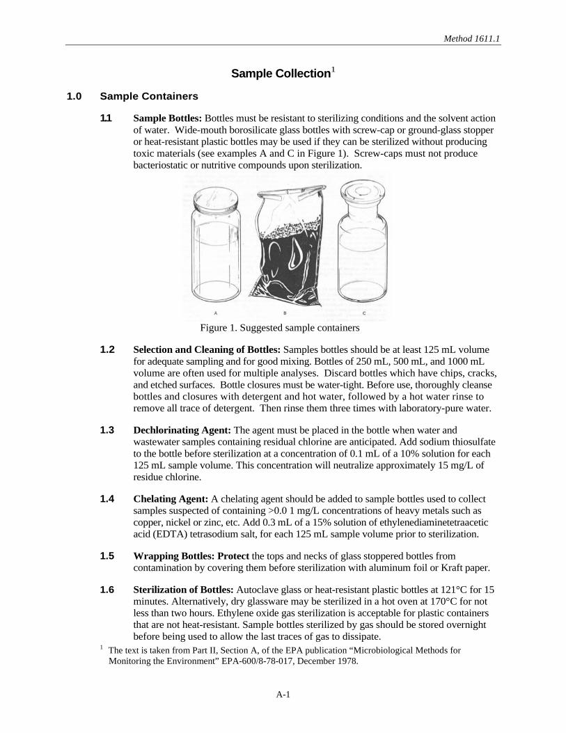
Method 1611.1

Sample Collection1

1.0 Sample Containers

1.1 Sample Bottles: Bottles must be resistant to sterilizing conditions and the solvent action of water. Wide-mouth borosilicate glass bottles with screw-cap or ground-glass stopper or heat-resistant plastic bottles may be used if they can be sterilized without producing toxic materials (see examples A and C in Figure 1). Screw-caps must not produce bacteriostatic or nutritive compounds upon sterilization.

Figure 1. Suggested sample containers

1.2 Selection and Cleaning of Bottles: Samples bottles should be at least 125 mL volume for adequate sampling and for good mixing. Bottles of 250 mL, 500 mL, and 1000 mL volume are often used for multiple analyses. Discard bottles which have chips, cracks, and etched surfaces. Bottle closures must be water-tight. Before use, thoroughly cleanse bottles and closures with detergent and hot water, followed by a hot water rinse to remove all trace of detergent. Then rinse them three times with laboratory-pure water.

1.3 Dechlorinating Agent: The agent must be placed in the bottle when water and wastewater samples containing residual chlorine are anticipated. Add sodium thiosulfate to the bottle before sterilization at a concentration of 0.1 mL of a 10% solution for each 125 mL sample volume. This concentration will neutralize approximately 15 mg/L of residue chlorine.

1.4 Chelating Agent: A chelating agent should be added to sample bottles used to collect samples suspected of containing >0.0 1 mg/L concentrations of heavy metals such as copper, nickel or zinc, etc. Add 0.3 mL of a 15% solution of ethylenediaminetetraacetic acid (EDTA) tetrasodium salt, for each 125 mL sample volume prior to sterilization.

1.5 Wrapping Bottles: Protect the tops and necks of glass stoppered bottles from contamination by covering them before sterilization with aluminum foil or Kraft paper.

1.6 Sterilization of Bottles: Autoclave glass or heat-resistant plastic bottles at 121°C for 15 minutes. Alternatively, dry glassware may be sterilized in a hot oven at 170°C for not less than two hours. Ethylene oxide gas sterilization is acceptable for plastic containers that are not heat-resistant. Sample bottles sterilized by gas should be stored overnight before being used to allow the last traces of gas to dissipate.

1 The text is taken from Part II, Section A, of the EPA publication “Microbiological Methods for Monitoring the Environment” EPA-600/8-78-017, December 1978.

A-1

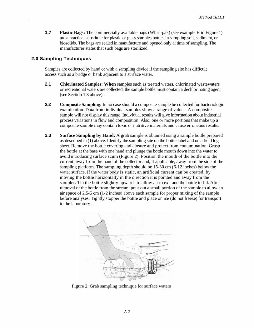
Method 1611.1

1.7 Plastic Bags: The commercially available bags (Whirl-pak) (see example B in Figure 1) are a practical substitute for plastic or glass samples bottles in sampling soil, sediment, or biosolids. The bags are sealed in manufacture and opened only at time of sampling. The manufacturer states that such bags are sterilized.

2.0 Sampling Techniques

Samples are collected by hand or with a sampling device if the sampling site has difficult access such as a bridge or bank adjacent to a surface water.

2.1 Chlorinated Samples: When samples such as treated waters, chlorinated wastewaters or recreational waters are collected, the sample bottle must contain a dechlorinating agent (see Section 1.3 above).

2.2 Composite Sampling: In no case should a composite sample be collected for bacteriologic examination. Data from individual samples show a range of values. A composite sample will not display this range. Individual results will give information about industrial process variations in flow and composition. Also, one or more portions that make up a composite sample may contain toxic or nutritive materials and cause erroneous results.

2.3 Surface Sampling by Hand: A grab sample is obtained using a sample bottle prepared as described in (1) above. Identify the sampling site on the bottle label and on a field log sheet. Remove the bottle covering and closure and protect from contamination. Grasp the bottle at the base with one hand and plunge the bottle mouth down into the water to avoid introducing surface scum (Figure 2). Position the mouth of the bottle into the current away from the hand of the collector and, if applicable, away from the side of the sampling platform. The sampling depth should be 15-30 cm (6-12 inches) below the water surface. If the water body is static, an artificial current can be created, by moving the bottle horizontally in the direction it is pointed and away from the sampler. Tip the bottle slightly upwards to allow air to exit and the bottle to fill. After removal of the bottle from the stream, pour out a small portion of the sample to allow an air space of 2.5-5 cm (1-2 inches) above each sample for proper mixing of the sample before analyses. Tightly stopper the bottle and place on ice (do not freeze) for transport to the laboratory.

Figure 2. Grab sampling technique for surface waters

A-2

Method 1611.1

3.0 Selection of Sampling Sites and Frequency

These will be described for streams, rivers, estuarine, marine, and recreational waters as well as domestic and industrial wastewaters.

3.1 Stream Sampling: The objectives of the initial survey dictate the location, frequency and number of samples to be collected.

3.1.1 Selection of Sampling Sites: A typical stream sampling program includes sampling locations upstream of the area of concern, upstream and downstream of waste discharges, upstream and downstream from tributary entrances to the river and upstream of the mouth of the tributary. For more complex situations, where several waste discharges are involved, sampling includes sites upstream and downstream from the combined discharge area and samples taken directly from each industrial or municipal waste discharge. Using available bacteriological, chemical and discharge rate data, the contribution of each pollution source can be determined.

3.1.2 Small Streams: Small streams should be sampled at background stations upstream of the pollution sources and at stations downstream from pollution sources. Additional sampling sites should be located downstream to delineate the zones of pollution. Avoid sampling areas where stagnation may occur (e.g., backwater of a tributary) and areas located near the inside bank of a curve in the stream which may not be representative of the main channel.

3.1.3 Large Streams and Rivers: Large streams are usually not well mixed laterally for long distances downstream from the pollution sources. Sampling sites below point source pollution should be established to provide desired downstream travel time and dispersal as determined by flow rate measurements. Particular care must be taken to establish the proper sampling points. Occasionally, depth samples are necessary to determine vertical mixing patterns.

3.2 Estuarine and Marine Sampling: Sampling estuarine and marine waters requires the consideration of other factors in addition to those usually recognized in fresh water sampling. They include tidal cycles, current patterns, bottom currents and counter-currents, stratification, seasonal fluctuations, dispersion of discharges and multi-depth samplings.

The frequency of sampling varies with the objectives. When a sampling program is started, it may be necessary to sample every hour around the clock to establish pollution loads and dispersion patterns. The sewage discharges may occur continuously or intermittently.

When the sampling strategy for a survey is planned, data may be available from previous hydrological studies done by the Coast Guard, Corps of Engineers, National Oceanic and Atmospheric Administration (NOAA), U.S. Geological Survey, or university and private research investigations. In a survey, float studies and dye studies are often carried out to determine surface and undercurrents. Initially depth samples are taken on the bottom and at five feet increments between surface and bottom. A random grid pattern for selecting sampling sites is established statistically.

A-3

Method 1611.1

3.2.1 Estuarine Sampling: When a survey is made on an estuary, samples are often taken from a boat, usually making an end to end traverse of the estuary. Another method involves taking samples throughout a tidal cycle, every hour or two hours from a bridge or from an anchored boat at a number of fixed points.

In a large bay or estuary where many square miles of area are involved, a grid or series of stations may be necessary. Two sets of samples are usually taken from an area on a given day, one at ebb or flood slack water, and the other three hours earlier, or later, at the half tidal interval. Sampling is scheduled so that the mid-sampling time of each run coincides with the calculated occurrence of the tidal condition.

In location sampling sites, one must consider points at which tributary waters enter the main stream or estuary, location of shellfish beds and bathing beaches. The sampling stations can be adjusted as data accumulate. For example, if a series of stations half mile apart consistently show similar values, some of these stations may be dropped and other stations added in areas where data shows more variability.

Considerable stratification can occur between the salt water from the sea and the fresh water supplied by a river. It is essential when starting a survey of an unknown estuary to find out whether there is any marked stratification. This can be done by chloride determinations at different locations and depths. It is possible for stratification to occur in one part of an estuary and not in another.

On a flood tide, the more dense salt water pushing up into the less dense fresh river water will cause an overlapping with the fresh water flowing on top. A phenomenon called a salt water wedge can form. As a result, stratification occurs. If the discharge of pollution is in the salt water layer, the contamination will be concentrated near the bottom at the flood tide. The flow or velocity of the fresh water will influence the degree of stratification which occurs. If one is sampling only at the surface, it is possible that the data will not show the polluted underflowing water which was contaminated at the point below the fresh water river. Therefore, where stratification is suspected, samples at different depths will be needed to measure vertical distribution.

3.2.2 Marine Sampling: In ocean studies, the environmental conditions are most diverse along the coast where shore, atmosphere and the surf are strong influences. The shallow coastal waters are particularly susceptible to daily fluctuations in temperature and seasonal changes.

Sampling during the entire tidal cycle or during a half cycle may be required. Many ocean studies such as sampling over the continental shelf involve huge areas and no two areas of water are the same.

Selection of sampling sites and depths are most critical in marine waters. In winter, cooling of coastal waters can result in water layers which approach 0°C. In summer, the shallow waters warm much faster than the deeper waters. Despite the higher temperature, oxygen concentrations are higher in shallow than

A-4

Method 1611.1

in deeper waters due to greater water movement, surf action and photosynthetic activity from macrophytes and the plankton.

Moving from the shallow waters to the intermediate depths, one observes a moderation of these shallow water characteristics. In the deeper waters, there is a marked stabilization of conditions. Water temperatures are lower and more stable. There is limited turbulence, little penetration of light, sparse vegetation and the ocean floor is covered with a layer of silts and sediments.

3.3 Recreational Waters (Bathing Beaches): Sampling sites at bathing beaches or other recreational areas should include upstream or peripheral areas and locations adjacent to natural drains that would discharge stormwater, or run-off areas draining septic wastes from restaurants, boat marinas, or garbage collection areas. Samples of bathing beach water should be collected at locations and times of heaviest use. Daily sampling, preferably in the afternoon, is the optimum frequency during the season. Weekends and holidays which are periods of highest use must be included in the sampling program. Samples of estuarine bathing waters should be obtained at high tide, ebb tide and low tide in order to determine the cyclic water quality and deterioration that must be monitored during the swimming season.

3.4 Domestic and Industrial Waste Discharges: It is often necessary to sample secondary and tertiary wastes from municipal waste treatment plants and various industrial waste treatment operations. In situations where the plant treatment efficiency varies considerably, grab samples are collected around the clock at selected intervals for a three to five day period. If it is known that the process displays little variation, fewer samples are needed. In no case should a composite sample be collected for bacteriological examination. The National Pollution Discharge Elimination System (NPDES) has established wastewater treatment plant effluent limits for all dischargers. These are often based on maximum and mean values. A sufficient number of samples must be collected to satisfy the permit and/or to provide statistically sound data and give a fair representation of the bacteriological quality of the discharge.

A-5

Method 1611.1

Appendix B: Life Technologies StepOnePlus™, Applied Biosystems AB 7900, and

AB 7500 Real-Time PCR System Operation

Method 1611.1

Appendix B: Life Technologies StepOnePlus™, Applied Biosystems AB 7900, and AB 7500 Real-Time PCR System Operation

1.0 Life Technologies StepOnePlus™

1.0.1 Turn on the StepOnePlus™ and then the computer. Launch the StepOnePlus™ software program by double clicking on its icon on the computer desktop or from the Computer Programs menu.

1.0.2 On the StepOnePlus™ home screen select Advanced Set Up.

1.0.3 On the right side of the main screen click in the box Experiment Name, enter identifying information for the experiment (Name/Date etc such that experiment can be identified). Then go through the following fields:

• Which instrument is going to be used to run the experiment: StepOnePlus™ Instrument (96 wells) is default (highlighted).

• What experiment do you want to set up: Quantitation-Standard Curve is default (highlighted).

• Which reagents will be used to detect the target: TaqMan® Reagents is default (highlighted).

• Which ramp speed do you want to use in the instrument run: Click on Standard-2 hours (Not Default)

1.0.4 Click on Plate Set Up from the navigational pane of the present screen to define the targets, and then assign them to wells in the reaction plate (Step 1.0.8).

1.0.5 Define target – You can add a new target or use a saved target. By clicking on Add Saved Target the window with the target library will open.

1.0.6 Select the target(s) for your assay(s) and click on Add Selected Targets. All of the targets may be selected simultaneously by holding the Ctrl key and highlighting the desired targets (e.g., Entero, Sketa). The selected targets will then be added on to the define target and sample screen.

1.0.7 Optional: If a new target is to be added click the Enter Target Name cell and type the name. From the Reporter dropdown menu, select FAM (default). From the Quencher dropdown menu, select TAMRA (NFQ-MGB) (default). Leave the default in the color field.

1.0.8 Click on the tab Assign Targets and Samples to see the screen view of the plate layout with 96 wells.

• Select the wells, based on the plate set up, by highlighting, one target at a time.

• Select the wells for the first target by checking the box for the desired target in Assign Target to the selected wells and it will automatically populate the wells for that target. If more than one target is being used, repeat the process above for each target.

• The wells can be selected individually or by rows by clicking in the left corner of the row. In addition, the whole plate may be selected by clicking in the left corner of the plate.

B-1

Method 1611.1

• To deselect a row or well press Ctrl & click the selected portion one more time and it will deselect the row or well. Selected wells/rows will be highlighted grey, while unselected wells/rows will remain white.

1.0.9 Run the Method 1.0.9.1 On the run method screen, review the reaction volume and the thermal profile for

the default run. If needed: The default run method can be edited or replaced with one from the run method library. Click either the Graphical view (default) or Tabular View tab.

1.0.9.2 Make sure the reaction volume per well field displays 25 µL, this is not the default setting.

1.0.9.3 Set the thermal profile to the following holding and cycling stages: Holding Stage 1: 50.0°C for 2:00 minutes, Holding Stage 2: 95.0°C for 10:00 minutes, Cycling Stage: 95.0°C for 0:15 seconds. The second step of the Cycling Stage is defaulted at 60.0°C for 1 minute. Use instrument default of 40 cycles.

1.0.9.4 Note: When using a run from the library click on the tab Open Run Method in the graphical view. Select Run Method and click ok. It will replace the default run with the saved run.

1.0.10 Load the plate into the instrument. 1.0.11 Click on the Plate Set Up tab and start the run by clicking the green button in the upper

right hand corner of the screen. 1.0.11.1 Save Experiment dialogue box − Click Save to accept default file name and

location (the name assigned when setting up the experiment). The experiment is saved by default to the <drive>:\ applied Biosystems\<software name>\experiment folder.

1.0.11.2 Run progress can be viewed from the touch screen of the instrument. At the beginning of a run do not leave the instrument or computer until you verify that the run has started.

1.0.12 Once the run is completed remove the reaction plate and discard. 1.0.13 Analyze the run

1.0.13.1 Click on the tab in the top right corner of screen to Analyze the Run. 1.0.13.2 Highlight all of the sample wells and click on Analysis Settings to get to CT

settings (default CT settings).

1.0.13.3 Highlight all the targets running in the plate; uncheck the default setting for automatic threshold and set the threshold to 0.03. Keep the Automatic Baseline. Click on Apply Analysis Settings to save changes. The new settings can be confirmed by viewing the threshold line on the amplification plot.

1.0.14 Press the Export tab on the left corner of the view plate layout screen. Click on the browse button to find the correct place to export the data and click Start Exporting. After the export is done close export tool.

1.1 AB 7900 Real-Time PCR System Operation 1.1.1 Turn on the AB Model 7900 and then the computer. Launch the SDS 2.2.2 software

program by double clicking on its icon on the computer desktop or from the Computer

B-2

Method 1611.1

Programs menu. The computer will establish communication with the 7900 instrument and if the connection is successful, the software will display the Connected icon in the status bar when a plate document is opened.

1.1.2 Under File menu, select New. 1.1.3 In resulting New Document window that appears, change container selection from 384

well clear plate to 96 well clear plate using drop down menu. Accept default selections of Absolute Quantification and Blank Template. Click OK to display a new plate document.

1.1.4 Click, hold and drag mouse over all PCR reaction tray wells containing samples in upper left window. Selected wells will be outlined with a bold line and their position numbers should appear in the results table in the lower left window. To unselect wells, repeat above process while holding down control key.

1.1.5 Above right hand window, click on Setup tab. 1.1.6 Before any analyses are performed, a specific detector for the method must be created.

Click on Add Detector button at the bottom of the setup screen. 1.1.7 Click on New in the pop-up window that appears. Another pop-up window will appear.

Under Name, type in a name for the detector that will be used by this method (e.g., “Method 1611”). Under Group select Default. Under Reporter select FAM and VIC. Under Quencher select TAMRA. Click on OK to close second pop-up window. This step only needs to be performed before the initial analysis run of the method. The detector that is named is selected in all subsequent analysis runs as indicated in step 1.1.8)

1.1.8 In pop-up window that was opened in step 1.1.7, select the desired detector under Names menu (e.g., Method 1611) and click on Copy to Plate Document button. Click on Done button to return to setup screen.

1.1.9 Click on Use box next to FAM (Entero and Sketa 22) VIC (IAC) detectors in right hand window. These boxes should become marked with an X. Name and color codes for FAM and VIC detectors should appear in each of the selected well positions in the upper left window and a data column for this detector should be created for each of the selected well positions in the results table in the lower left window.

1.1.10 Click on Instrument tab right hand window. 1.1.11 In instrument screen, change sample volume to 25 μL and choose 9600 emulation. 1.1.12 Still in instrument screen, click on Connect, then click on Open/Close button in lower

right hand “Real Time” window to open PCR reaction tray holder door on instrument. 1.1.13 Insert PCR reaction tray with prepared reactions in holder. 1.1.14 Click on Open/Close button to close PCR reaction tray holder door on instrument. 1.1.15 Click on Start button in lower right hand “Real Time” window to start thermal cycling in

instrument. 1.1.16 Name run file at prompt. 1.1.17 At termination of the run, instrument-calculated cycle threshold (CT) values should

automatically appear for each well position and detector entry in the lower left hand results table window.

B-3

Method 1611.1

1.1.18 At termination of the run success complete, choose Analysis Settings from the toolbar. In that box enter a value for the Manual CT Threshold (see 1.0.13.3). Click on OK. Click on Analyze from the toolbar. You should see CT values in the Results Table.

1.1.19 The instrument-selected threshold line is indicated by the bold red line on the plot and the value is listed below the window. This can be manually adjusted by either click-hold and dragging the line up or down or entering new values below. Note: Based on results thus far with the instrument, the threshold value can be adjusted from the default value of 0.2 to 0.03, however, this should be done only if the threshold line remains above the background values (seen before the growth curves) for all of the samples.

1.1.20 Calculated CT values for each of the sample tray positions in the lower left hand “Results Table” will automatically be updated following adjustments of the threshold line. Once the threshold is adjusted to the desired level, select “Print Report” under the “File” menu. Check or uncheck desired report items by clicking on their associated boxes and the click on “Print” button. Note: Minimum report should have both detector boxes, i.e., “FAM” checked which will show CT values for all selected tray positions for this detector.

1.1.21 Export data by clicking on File from the toolbar. From the drop down menu choose Export. In the box you will see Look in: and here you choose a directory to send the exported file too. Click on Export. Save changes to document? will appear, click on Yes. Click OK.

1.2 AB 7500 (non-Fast) Real-Time PCR System Operation 1.2.1 Turn on the AB Model 7500 and then the computer. Launch the software program by

double clicking on its icon on the computer desktop or from the Computer Programs menu. The computer will establish communication with the 7500 instrument. See “How to Set Up a New Experiment Using the AB 7500” for screen shots.

1.2.2 Click on either the New Experiment or Advanced Setup button to create a new experiment, which will pull up the Experiment Menu.

1.2.3 From the Setup menu, select Experimental Properties to select the experiment type and give the experiment a name. Enter the experiment name in the asterisked box. 1.2.3.1 Click on 7500 (96 Wells) to select the instrument type. Note: This protocol

is not designed for the 7500 Fast. 1.2.3.2 Scroll down to access more experiment properties options. Click on

Quantitation – Standard Curve to select the experiment type. 1.2.3.3 Click on TaqMan® Reagents to select the reagents used.

1.2.4 From the Setup menu, select Plate Setup. Click on the Define Targets and Samples tab to define the reporter-quencher dye for each target and also to enter the sample identifications (e.g., Ent 5X).

1.2.4.1 Click on Add New Target and enter the name of the target. Under the Reporter heading, click on the drop down menu to select the reporter dye FAM (Entero and Sketa 22) and VIC (IAC). Under the Quencher heading, click on the drop down menu to select TAMRA as the quencher.

1.2.4.2 Repeat the process in Section 1.2.4.1 to add more than one target, e.g., Sketa 5x.

1.2.4.3 In the Define Samples section, click on Add New Sample and enter the sample name in the Sample 1 box.

B-4

Method 1611.1

1.2.4.4 Click on the Assign Targets and Sample tab to assign the Target, sample ID and sample type to the wells.

1.2.4.5 Drag the mouse over the desired cells to assign the Target, Task and Sample.

1.2.4.6 While the cells are highlighted, in the Assign target(s) to the selected wells section, check the box under Assign for the appropriate Target, then under Task, select U for unknown, S for standard or N for negative control.

1.2.4.7 In the Assign sample(s) to the selected wells section, check the box under Assign to label the highlighted cells as Sample 1 (e.g.).

1.2.4.8 Repeat the process in Section 1.2.4.4, dragging the mouse over the appropriate cells, and then assigning them as Unknowns, Standards or Negative Controls, as appropriate. Note that for the Standards, in the Assign target(s) to the selected wells section, if there are 4 different values, each cell will need to be highlighted separately, and a quantity (e.g., 40000.0) typed in the Quantity box.

1.2.4.9 Click on Print Report at the top of the screen to print a plate layout for loading master mix and sample extracts. 1.2.4.9.1 Select Plate Layout option by clicking on the box next to it.

1.2.4.9.2 Click Print Report to print the plate layout. 1.2.5 From the Setup menu, select Run Method to set up the thermo cycling profile.

1.2.5.1 In the Graphical View tab, change the Reaction Volume Per Well from the default 50 μL to 25 μL by typing in 25.

1.2.5.2 Under Cycling Stage section, change the Number of Cycles to 45.

1.2.5.3 Check that the default settings of Temperature and Time for the two Holding Stages and the Cycling Stage are correct. Specifically, these should be: Holding Stage 1: 50.0°C for 1:00 minute, Holding Stage 2: 95.0°C for 10:00 minutes, and Cycling Stage: 95.0°C for 0:15 seconds.

1.2.5.4 The second step of the Cycling Stage is defaulted at 60.0°C for 1 minute. Note: This sets the detection of the fluorescence signal to occur at the end of the second step in each cycle.

1.2.5.5 Click on Save at the top of the screen to save the run before actually running the experiment.

1.2.5.6 The Save screen will open so that you may select the folder to save the Run Data File. Type in the Experiment Name (if you did not already do so at the beginning of the Experiment Setup) and click on Save. If you had previously typed in an Experiment Name and there is no change, click on Save. Note: You must save to the hard drive (rather than a flash drive).

1.2.6 From the Experiment menu, select Run to monitor the run in real time.

1.2.6.1 The Run Status screen will open - click on Start Run. When the run has successfully started, the Start Run button will turn change from green to red.

1.2.7 When the run has completed, from the Setup menu, select Analysis to export your results. See “How to Export Results from the AB 7500 Software” for screen shots. 1.2.7.1 The Analysis Settings for Experiment name screen will open.

B-5

Method 1611.1

1.2.7.2 Under the CT Settings tab, click on the Target desired to be set from Default to Manual Threshold setting (generally, this would be the Ent).

1.2.7.3 In the CT Settings for ENT section, uncheck the boxes next to Use Default Settings, and Automatic Threshold. Enter the desired Threshold (e.g., 0.025). If more than one target is present, highlight the next target (e.g., Sketa) and repeat this step.

1.2.7.4 Click on Apply Analysis Settings to save the changes.

1.2.8 Click on Export at the top of the screen to save the experiment results data and to save the selected plots required in the report. Note that the threshold value will have changed on the Amplification plot curve graphic. 1.2.8.1 The Export Data screen will open. In the Select data to export section,

check all of the boxes (i.e., Sample Setup, Raw Data, Amplification Data, Results, and Multicomponent Data).

1.2.8.2 For Select one file or separate files, select One file to export all the data into one file with multiple tabs.

1.2.8.3 For Export File Name, enter the name of the Experimental data file to be exported, and for File Type, choose *.xls.

1.2.8.4 For Export File Location, click on Browse to select the folder in which you wish to export your file. Always save your file to the hard drive.

1.2.8.5 Click on Start Export. When this is completed, an Export Completed screen will open – click on Close Export Tool to complete this task.

1.2.9 How to interpret your results. See “How to Interpret Results from the AB 7500” for screen shots.

1.2.9.1 After exporting your data, from the Experiment menu, select Analysis. 1.2.9.1.1 From the Analysis menu, select Amplification Plot to view the

results of the selected samples at different plot settings. 1.2.9.1.2 Drag the mouse over the desired cells to select the samples to be

plotted in the amplification plot. 1.2.9.1.3 In the Amplification Plot section, in the Plot Settings tab, select

the Plot Type (from the drop down menu) and the Graph Type (from the drop down menu).

1.2.9.1.4 If the plot requires the display of the Threshold and Baseline, in the Options tab, check the boxes next to Threshold and Baseline. If you want to see the results in tabular format, click on View Well Table, and scroll down or sideways for more samples and analysis parameters.

1.2.9.1.5 The toolbar above the graph can be used to make hard copy prints, saving the file as *.jpg, zooming in and out, and changing the plot properties.

1.2.9.2 For the Standard Curve, select Standard Curve from the Analysis menu to view the results of the same sample (assuming they have the same target) and standards in the plot.

B-6

Method 1611.1

1.2.9.2.1 In the Plot Settings tab, click the drop down menu arrow beside Target to select a different target (if the standards were analyzed in more than one target), and click the drop down menu arrow beside Plot Color to change the plot color.

1.2.9.2.2 The standard curve parameter display below the plot (i.e., Target, Slope, Y-Inter(cept), R2, and Eff% (percent efficiency) is useful for data analysis.

1.2.9.3 For Multicomponent plots, click on Multicomponent Plot from the Analysis menu to view the variation in the fluorescence of the dyes used in the experiment over the ascending repeat of the 40 thermo cycles based on well, target, or dye.

1.2.9.4 Click on the drop down menu arrow next to Plot Color in the Plot Settings tab to select the parameter for the basis of the graph (e.g., well, target, or dye).

1.2.9.5 For raw data plots, select Raw Data Plot from the Analysis menu to view the variation in the emission of fluorescence of the dyes in different filters present over the ascending repeat of the 40 thermo cycles.

1.2.9.6 In the Options tab, drag the pointer on the cycle scale to the desired cycle number to view the fluorescence variation through filters of the samples at that cycle.

1.2.9.7 For quality controls, click on QC Summary from the Analysis menu to view the analysis summary of the samples.

1.2.9.8 To view all the plots, click on Multiple Plots View from the Analysis menu to see all of the plots for the samples in a single window. Each plot will have its own drop down menu.

1.2.10 To print the report, click on Print Report at the top of the screen.

1.2.10.1 Check all of the boxes (i.e., Experimental Summary, Results Summary, Plate Layout, Amplification Plot (3 boxes), Standard Curves, Results Table, and QC Summary).

1.2.10.2 Click on Print Report at the bottom of the screen.

B-7

Method 1611.1

Appendix C: Cepheid Smart Cycler® Operation

Method 1611.1

Appendix C - Cepheid Smart Cycler® Operation 1.0 Smart Cycler® Operation 1.1 This protocol is intended to provide only information about critical instrument settings required to

perform EPA Method 1611.1. Further details concerning the operation of the instrument can be obtained from the Smart Cycler® Operation Manual, Cepheid Part D0190, Rev. D.

1.2 Turn on the Smart Cycler®; then the computer. 1.3 Double-click on the Smart Cycler® icon on the computer desktop. 1.4 The following steps for defining a protocol are only required before the initial run of the

instrument. The protocol that is defined in these steps is used in all subsequent runs of the instrument. See “How to Set Up a New Experiment Using the Smart Cycler® (Software Version 2.0” for screen shots. 1.4.1 Click on the Define Protocols icon to go to Define Protocols screen. 1.4.2 Click on the New Protocol button to open the Protocol Name? dialog. Enter “EPA

Enterococcus Method 1611” for the new protocol name, and click OK. The protocol stages are defined in the series of boxes at the bottom of the Define Protocol screen. Make sure the new protocol is highlighted and begin to choose state settings. To define Stage 1, click on its drop-down box to display the menu of stage types; then select Hold. In the Temp column, enter 50.0, and in Secs column, enter 60, leaving the Optics setting as the default Off setting.

1.4.3 To define Stage 2, click on its drop-down box to display the menu of stage types, and again select Hold. In the Temp column, enter 95.0, and in Secs column enter 600. Again, leave the Optics setting on Off.

1.4.4 To define Stage 3, select 2-Temperature Cycle from its drop down menu. For the first step, enter 95.0 in the first row of the Temp column and 15 in the Secs column, Optics column Off. For the second step, enter 60.0 in the second row of the Temp column, 60 in the Secs column, and click on the Optics cell to select On from the drop-down menu. (Note: This sets the detection of the fluorescence signal to occur at the end of the second step in each cycle.) Enter 40 in the Repeat field at the top of the Stage 3 box to specify that it should be repeated for 40 cycles. Click the Save Protocol button.

1.4.5 To display primary curve graphs, click Define Graphs. Highlight FAM and VIC in Graph column. Check the box for Automatically add to new runs. Under Graph Type choose Optics from the pull down menu. Under Channels check the box for Ch 1 (FAM) and Ch 2 (VIC). Under Show check the boxes for Primary Curve, Threshold (Vertical) and Threshold (Horizontal). Under Axes check the box for Fluorescence vs. Cycle. At the bottom of the screen click on Save Graph.

1.5 Click on the Create Run icon to open the Create Run screen. For each new run, enter a unique name in the Run Name field. (Note: The software does not allow duplicate run names).

1.6 Enter any additional information about the run in the Notes field. Click the arrow in the Dye Set box to display a drop-down menu of the possible selections. Select FTTC25. (Note: This selects the dye set: FAM, TET, Tex Red, Cy5, and a 25 μL reaction).

1.7 Click the Add/Remove Sites button. The Select Protocols and Sites... dialog will appear. Highlight (click on) the "EPA Method 1611" protocol developed prior to the first run (Section 1.4.2) in the Protocols list. In the Sites list, highlight the sites on the instrument to be used with this protocol in the current run by clicking on them with the shift key held down (Note: Sites refer

C-1

Method 1611.1

to the I-core modules in the Smart Cycler® processing block in which reaction tubes will be placed; a total of 16 are possible per block. When using multiple blocks, the site numbers will be preceded by the block letters, e.g., A, B, C); then click the right pointing arrow to transfer the selected sites and protocol to the Selections table.

1.8 Click on the OK button to save the selections, and return to the Create Run screen. 1.9 Place the loaded Smart Cycler® reaction tubes in the I-core module slots, selected above for

current run. The tubes should snap into place. Either the front or back of the caps can face the front of the processing block.

1.10 In one of the View menus that is shown, select Analysis Settings. The displayed table includes one row for each of the four possible dye channels defined in the dye set. Click on the cell in the FAM row under the Usage column heading, and select Assay from the drop down menu. Set the Usage cells for VIC in the same manner. (Note: All assays in this protocol use FAM and VIC as the reporter dye). All other cells in this table should be left at default settings (See Smart Cycler® Operation Manual).

1.11 In the other View menu that is shown, select the Results Table. Enter the sample identification information for each site in the Sample ID column (additional information can be entered into the Notes column.). Leave the other columns as default settings (see Smart Cycler® Operation Manual.).

1.12 Click on the Start Run button. The orange LEDs on the Smart Cycler® processing block should turn on, and the software will automatically switch to the View Results screen.

1.13 To display the real time temperature profiles for all sites, click Temperature in either of the View menus. To display real time growth curves for all samples (i.e., the fluorescence signal vs. cycle), click FAM and VIC in the other View menu.

1.14 At the end of the run, it is recommended to check the cycle threshold values calculated by the instrument for each sample by opening the Results Table window by clicking on this selection in the upper View menu. It is also recommended to inspect the growth curves in the FAM window and in the VIC window which can be opened in the same manner from the lower View menu. The default threshold fluorescence value is shown in this window as a single horizontal red line and the cycle thresholds for each site are shown as vertical red lines. To view the data for individual sites in this window, click on that site number in the table to the right of the graph. If the default threshold fluorescence line is well above all of the growth curve lines prior to visible amplification, the threshold fluorescence value can be changed to a lower value. This is done by reopening the Analysis Settings window from the upper View menu and entering a new value in the Manual Thresh Fluor Units cell in the FAM row and VIC row. Conversely if the default threshold fluorescence line is below any of the growth curve lines prior to visible amplification, the threshold fluorescence value should be changed to a higher value in the same manner. Previous studies have indicated that a threshold value of 8 works well for most analyses. Click on the Update Analysis button to view the new threshold line in the FAM window and VIC window. The cycle threshold values will be automatically updated in the Results Table.

1.15 Once the threshold fluorescence value is adjusted to an optimal value, click the Save Run button. (Note: The Smart Cycler® Software does not give a prompt to save changes before printing or exporting. Therefore, it is possible to make changes to the Results Table or Analysis Settings, and immediately print or export the data, then close the run without saving the changes. In this case, the data saved in the Smart Cycler® database will not match the printed or exported data. If no changes are made in the threshold fluorescence value, the run data is automatically saved as it is when the program is closed or a new run is created).

C-2

Method 1611.1

1.16 To set up automatic export of raw data, (see “How To Set Up Automatic Export of Raw Data” for screen shots) from the main menu, click on Setup, then System Defaults, then Export Settings. From the Export Settings dialog box, check the box beside Results Table and Analysis Settings. Click the Browse button to select the folder where you want your raw data saved. Click on the radio button next to Automatic export on run completion, then click the OK button.

1.17 To manually save the Results Table and Analysis setting containing the instrument-calculated cycle threshold values for each sample (see “How to Manually Export Raw Data” for screen shots), click the Export button to display the Export Data dialog box. Check the box next to the heading Export Results Table and Analysis Settings by clicking on it. Leave all other boxes unchecked. Click on Export. A box labeled Export Data will appear with the run name in the file name box. Click on the drop down menu to the right of Save In: at the top left of the screen to change the directory where you want your data saved. Click on Save. Data are exported as comma-delimited text (*.cvs) files in MS Excel-compatible files to the Export folder in the Smart Cycler® folder: C:\Smart Cycler®\Export. Always save to the hard drive.

1.18 To archive a run in the Smart Cycler® program, click on Tools. From the drop down menu click

on Data Management and then Archive Runs. Click Proceed. Select the run to be archived by clicking on its name in the database list. Click OK and then Proceed. A box labeled Archive Run will appear on the screen. There will be a line labeled Save in: Input which directory you would like the run to be saved in. There will be a line File Name: Enter a file name. Click Save. Click OK.

1.19 To print run data (see “How to Print Run Data” for screen shots), after the run is completed, right

click on the graph area, and select Print, then Print Graph with Results Table. An Optics Graph print preview screen will pop up, click Print. The screen will switch back to the post run screen. To print the generated report, click Report. A Run Report print preview screen will pop up, click Print.

1.20 To set up a new analysis (see “How to Set Up a New Run” for screen shots), from the post run

screen, click Create Run at the top left. The results of your just completed will disappear and a Add/Remove Sites button will appear in the middle of the screen – click it. A Select Protocols and Sites screen will pop up, select EPA Enterococcus Method 1611 in the Protocols box, and highlight the amount of sites needed for the assay (A1-A16) in the Sites box. Click the right arrow to the right of the sites box to move the sights to the Selections box. After double checking that the correct protocol is highlighted, click OK. Add the Run Name in the Run Name box. The Site ID, Protocol, Sample ID, Sample Type, Notes (etc.) box will pop up. Enter the Sample ID for each site. Under this box, find the Usage column and click on Assay to select Unused for Cy3, TxR and Cy5 (leave Assay for FAM). In the same box, find the Manual Thresh Fluor Units, and click on the units for FAM to change it from 30.0 to 8.0 (leave the units at 30.0 for Cy3, TxR and Cy5). After loading the Smart Cycler® with tubes, click Start Run. A red light should appear on sites that are in use.

C-3

Method 1611.1

Appendix D: Protocol for MPN Estimation of DNA Standard Concentrations

Method 1611.1

Appendix D: Protocol for MPN Estimation of DNA Standard Concentrations

Initial qPCR analysis for negative control

1. Prepare master mix containing primer/probe working stock for Entero1A assay, BSA and 2x ABI Universal Master Mix for sufficient reactions and transfer 24 – 20 µL aliquots to 96 well reaction plate.

2. Add 5 µL AE buffer to each well containing master mix and cover plate with optical adhesive tape

3. Run reactions using ABI instrument default thermal cycling conditions for 45 cycles 4. At completion of run, set instrument fluorescence threshold to 0.03 and inspect results for

frequency of positive wells (wells giving CT values as opposed to “undetermined”) a. Frequency of positive wells should either be zero or very low for MPN analysis. If

frequency of positives is > 25%, there is unacceptable contamination of reagents to perform MPN analysis. Repeat using a different lot of Universal Master Mix.

First DNA qPCR analysis 5. Dilute genomic DNA or linearized plasmid stock solution in AE buffer to presumptive

concentration of 4 × 105 copies/5 µL based on estimated target sequence concentration of the DNA stock solution determined as described in Section 11.2 (genomic DNA) or Section 7.23 (plasmid DNA).

6. Perform 10-fold serial dilutions of presumptive 4 × 105 copies/5 µL sample from step 5 with AE buffer to make DNA standards with presumptive 4 × 104 copies/5 µL, 4 × 103 copies/5 µL, 4 × 102 copies/5 µL and 4 × 101 copies/5 µL. Note: Perform dilutions in low retention micro-tubes (see Section 6.24).

7. Prepare master mix containing primer/probe working stock for Entero1A assay, BSA and 2x ABI Universal Master Mix for sufficient reactions and transfer 24 – 20 µL aliquots to 96 well reaction plate.

8. Add 5 µL of presumptive 4 × 104 copies/5 µL, 4 × 103 copies/5 µL, 4 × 102 copies/5 µL, 4 × 101 copies/5 µL standards and AE buffer to 4 wells each containing master mix and cover plate with optical adhesive tape.

9. Run reactions using ABI instrument default thermal cycling conditions for 45 cycles. 10. At completion of run, set instrument fluorescence threshold to 0.03 and record CT values. 11. Perform regression analysis of CT values on log10 copies/well as described in Section 9.10.

Second DNA qPCR analysis

12. Perform 2-fold serial dilutions of presumptive 4 × 101 copies/5 µL standard in AE buffer to make 2 × 101 copies/5 µL, 1 × 101 copies/5 µL, 5 × 100 copies/5 µL, 2.5 × 100 copies/5 µL, 1.25 × 100 copies/5 µL and 0.625 × 100 copies/5 µL. Note: Perform dilutions in low retention micro-tubes (see Section 6.24).

13. Prepare master mix containing primer/probe working stock for Entero1A assay, BSA and 2x ABI Universal Master Mix for sufficient reactions and transfer 96 – 20 µL aliquots to two - 96 well reaction plates.

D-1

Method 1611.1

14. Add 5 µL of presumptive 2 × 101 copies/5 µL, 1 × 101 copies/5 µL, 5 × 100 copies/5 µL and AE buffer to 24 wells each of the first plate containing master mix and cover plate with optical adhesive tape.

15. Add 5 µL of presumptive 2.5 × 100 copies/5 µL, 1.25 × 100 copies/5 µL, 0.625 × 100 copies/5 µL and AE buffer to 24 wells each of the second plate containing master mix and cover plate with optical adhesive tape.

16. Run reactions using ABI instrument default thermal cycling conditions for 45 cycles. 17. At completion of run, set instrument fluorescence threshold to 0.03 and record CT values. 18. Record number of wells giving positive CT values as opposed to “undetermined” for each dilution

of the presumptive 4 × 101 copies/5 µL standard (and for AE buffer on each plate if applicable). Note: At least 3 of the dilutions should give a mixture of positive and negative results in the 24 replicate reactions. If this is not the case, it may be necessary to repeat the experiment with even higher dilutions of the presumptive 4 × 101 copies/5 µL standard (i.e., if all wells are giving positive results) or beginning with dilutions from the presumptive 4 × 102 copies/5 µL standard (i.e., if all wells are giving negative results)

Statistical analyses 19. Starting with lowest dilution where some wells give negative results, type number of positive

wells in cell C3 of MPN calculation spreadsheet. Note: If any AE wells on same plate are positive, type following formula in cell C3: = ((number of positive wells for dilution - number of positive wells for AE) / (24 - number of positive wells for AE)) x 24

20. Repeat previous step, typing number of positive wells (or formula) from progressively higher dilutions of the standard in cells C4, C5, C6 etc. up to the highest dilution where any wells are positive (or outnumber positive AE wells on corresponding plate)

21. Type the value 24 in each row of column B corresponding to rows in column C that contain values.

22. Calculate the fraction of the volume of the presumptive 4 x 101 copies/5 µL standard from step 6 that was added to the reactions corresponding to the lowest dilution giving usable data as described in step 19 (e.g., if usable data started with a two-fold dilution of this standard, the calculated value would be 0.5; if usable data started with a four-fold dilution of this standard, the value would be 0.25; if usable data started with an eight-fold dilution of this standard, the value would be 0.125; etc. Type this initial value in cell A3. Type 0.5 x this value in cell A4; 0.25 x this value in cell A5, 0.125 x this value in cell A6, etc, corresponding to each row in column C that contain values.

23. Type the number that then appears in cell J3, into cell G2. Hit Enter key. 24. Then hold down Ctrl key and type "m". Correct MPN (cell G2) logMPN (cell G3), and low and

high 95% confidence limits (cells G7-H8) will now be displayed. 25. Also check value in cell J16 to confirm test assumptions have not been violated (improbability

ratios > 1.00E-04 are considered acceptable in the spreadsheet but available results suggest improbability ratios should be < 1.0E-01)

26. The displayed MPN (cell G2) logMPN (cell G3) values are your corrected estimates of the target sequences/5 µL of the presumptive 4 × 101 copies/5 µL DNA standard from step 6.

D-2

Method 1611.1

Additional DNA qPCR and statistical analyses 27. To increase confidence in the MPN estimate, it is recommended that the analysis indicated above

should be repeated at least twice (3 replicate runs total). These additional runs only need to be performed using the three lowest dilutions that all gave both positive and negative results in different wells in the initial analysis (if lowest such dilution gives close to 100% positives (e.g., > 20/24), avoid this dilution and start with the next dilution to reduce possibility of 100% positives in some of the replicate runs). EPA data suggests that the coefficient of variation in the MPN estimates from these multiple runs should not exceed ~30%. Assuming similarity of results from run to run, the MPN estimates from each experiment can be averaged to calculate a final mean MPN estimate.

28. To characterize uncertainty by statistical analysis, the analysis should be repeated at least 5 additional times (total of at least 6 replicate runs) (Note: Statistical analysis of uncertainty is not discussed in detail in this guidance. See Reference 16.6 for further guidance).

29. Assuming the standard curve(s) performed in step 9 meet the acceptability criteria for slope specified in Section 9.10, the final MPN target sequences/5 µL estimate for the presumptive 4 × 101 copies/5 µL DNA standard also can be used to obtain corrected concentration estimates of the other 3 standards prepared in step 6 simply by multiplying by the dilution factors, e.g., 10x, 100x and 1000x.

D-3

Method 1611.1

Appendix E: How to Obtain DNA Standards from EPA

Method 1611.1

Appendix E: How to obtain DNA standards from EPA

A. What we need from you: 1. Please email your request to Robin Oshiro at Oshiro.robin@epa.gov 2. Please put "Request for EPA DNA standards" in the subject line (so that your request does not

inadvertently go into a junk folder). 3. Please provide the following information:

a. Your name, phone number and email address b. The name, phone number, and email address of the person to whom the DNA standards will

be shipped, if different from (3a) c. Your institution (e.g., company name) d. Your courier address (i.e., Federal Express address, which may be different from your U.S.

Postal Service mail delivery address) 4. Please note that:

a. We cannot ship to residential addresses b. We cannot ship the DNA standards if you do not provide all of the information required (see

[3] above) c. We are not responsible for incorrect addresses resulting in inability to deliver. If a box is

returned to us, we cannot ship you another box. Therefore, please double check your information before sending it.

5. Once we have emailed you the Federal Express tracking number, please verify receipt of that information via email.

B. What we will do: 1. Your request for DNA standards will be acknowledged as soon as possible via email. Once the

verification email is sent to you, with very few exceptions, we cannot change any information for the shipping label. Therefore, it is vital that you verify your information before sending it to us.

2. We will ship a set of five DNA standards to you on dry ice. Lot-specific concentration information will be provided with each kit.

3. We expect to ship only on Tuesdays. This is so that if there is any courier holdup, you can still receive your standards before the end of the week. In most cases, you should expect your box to arrive the next business day. a. If Monday or Tuesday is a U.S. Government federal holiday or the federal government is

closed in the DC metro area, your shipment will be made the following week. 4. We use Federal Express. We are not responsible for courier inability to deliver on time due to,

for example, inclement weather or other mishaps. 5. We will email you the tracking number of your box.

C. Restrictions (other than those stated above)

1. The DNA standards will be available until December 2015. 2. Only one set of DNA standards can be sent per laboratory per year (i.e., one set in 2015). 3. The DNA standards can only be sent to addresses in the United States and Territories (all 50

states, American Samoa, District of Columbia, Guam, Northern Mariana Islands, Puerto Rico, United States Minor Outlying Islands, and United States Virgin Islands). We cannot ship the standards outside the United States.

E-1