Earth Syst. Sci. Data, 12, 741–752, 2020https://doi.org/10.5194/essd-12-741-2020© Author(s) 2020. This work is distributed underthe Creative Commons Attribution 4.0 License.

Meteorological drought lacunarity aroundthe world and its classification

Robert Monjo1,2, Dominic Royé3,4, and Javier Martin-Vide5

1Climate Research Foundation (FIC), C/Gran Vía 22 (duplicado), 7, 28013 Madrid, Spain2Department of Algebra, Geometry and Topology, Complutense University of Madrid,

Plaza Ciencias, 3, 28040 Madrid, Spain3Department of Geography, University of Porto, Via Panorâmica, 4150-564 Porto, Portugal

4Department of Geography, University of Santiago de Compostela, Praza da Universidade 1,15782 Santiago de Compostela, Spain

5Climatology Group, Department of Physical Geography, University of Barcelona,C/Montalegre 6, 08001 Barcelona, Spain

Correspondence: Robert Monjo (robert@ficlima.org)

Received: 3 July 2019 – Discussion started: 26 August 2019Revised: 4 February 2020 – Accepted: 29 February 2020 – Published: 27 March 2020

Abstract. The measure of drought duration strongly depends on the definition considered. In meteorology, dry-ness is habitually measured by means of fixed thresholds (e.g. 0.1 or 1 mm usually define dry spells) or climaticmean values (as is the case of the standardised precipitation index), but this also depends on the aggregationtime interval considered. However, robust measurements of drought duration are required for analysing the sta-tistical significance of possible changes. Herein we climatically classified the drought duration around the worldaccording to its similarity to the voids of the Cantor set. Dryness time structure can be concisely measured bythe n index (from the regular or irregular alternation of dry or wet spells), which is closely related to the Giniindex and to a Cantor-based exponent. This enables the world’s climates to be classified into six large typesbased on a new measure of drought duration. To conclude, outcomes provide the ability to determine whendroughts start and finish. We performed the dry-spell analysis using the full global gridded daily Multi-SourceWeighted-Ensemble Precipitation (MSWEP) dataset. The MSWEP combines gauge-, satellite-, and reanalysis-based data to provide reliable precipitation estimates. The study period comprises the years 1979–2016 (total of45 165 d), and a spatial resolution of 0.5◦, with a total of 259 197 grid points. The dataset is publicly available athttps://doi.org/10.5281/zenodo.3247041 (Monjo et al., 2019).

1 Introduction

Drought depends mainly on the sector affected and thetimescale considered (Wilhite and Glantz, 1985; Crausbayet al., 2017). Focusing on the timescale, we usually dis-tinguish between dry spells (daily timescale) and negativeanomalies, commonly represented by monthly or yearly in-dices such as the standardised precipitation index, the stan-dardised evapotranspiration index, or the Palmer droughtseverity index, among others (Vicente-Serrano et al., 2010,2015). Alternation between dry and wet events presents self-similarity (characteristic of fractal objects) in the same man-

ner that the Cantor set alternates points with gaps (Martínezet al., 2007; Feng et al., 2015; Dayeen and Hassan, 2016;Lucena et al., 2018). According to Mandelbrot, fractality canbe found by measuring. He noted that, the more accurate themeasurement ruler, the more infinite the British coastline ap-pears to be, since the immeasurable curves of the coast situateit between a line (one dimension) and a surface (two dimen-sions), i.e. with a fractal or fractional dimension (Mandel-brot, 1967).

A commonly used method for measuring the dimensionof fractal objects involves box counting, which is similar to

Published by Copernicus Publications.

742 R. Monjo et al.: Drought to last longer than previously thought

using a ruler for measuring a coastline. Given an object em-bedded in an N volume (N = 1, length; N = 2, area; N = 3,volume; etc.), the method consists of covering the objectseveral times, using unitary (N − 1)-volume boxes of differ-ent sizes r for each completed covering, and counting howmany covering boxes are required in each case (Olsson et al.,1992; Sakhr and Nieminen, 2018). As the box size becomessmaller, the total (N − 1) volume of the fractal object tendstowards the infinite rather than converging towards a finervalue, and the N volume is zero. For instance, the Cantorset is embedded in the [0, 1] segment with infinite (zero-dimensional) points, but its total (one-dimensional) length iszero. Formally, an object (embedded in an N volume) pos-sesses a fractal (non-integer) dimension B between N − 1and N if a well-defined B volume V =Mrr

B exists, whereMr is the number of boxes with size r (Imre and Bogaert,2006). A well-defined B volume means that V and B remainconstant for small values of r .

Another related measure involves the Lyapunov expo-nent, which indicates the rate of separation of infinitesimallyclose trajectories, or involves the inverse, sometimes referredto as Lyapunov time, since it indicates the time expectedto become a chaotic trajectory (Boeing, 2016; Kuznetsov,2016; Gaspard, 2005; Bezruchko and Smirnov, 2010). TheHurst exponent is also related to the fractal dimension ofchaotic time series, providing possible long-term memorythroughout autocorrelation (Mandelbrot, 1985; Feder, 1988;Yu et al., 2015).

The fractal behaviour of dry spells can be observed inRichardson’s log–log plot of cumulative dry durations withregard to different unit durations (Sen, 2008; Meseguer-Ruizet al., 2017). Similarities with the Cantor set (positive Lya-punov exponents) were found for dry-spell sequences in Eu-rope (Lana et al., 2010). In this sense, dry pauses of therainfall can be compared with the gap distribution of fractalobjects, which is also known as lacunarity (Martínez et al.,2007; Lucena et al., 2018). The lacunarity analysis is usedto characterise “spatial” patterns (such as invariance, density,and heterogeneity) of fractal objects, which represent attrac-tor solutions of nonlinear dynamical systems (Plotnick et al.,1996; Wilkinson et al., 2019). If a time series of precipita-tion is a solution of the climatic system at a given point, thedryness distribution informs (climate) average features of thesystem (e.g. surface convergences or divergences of moistureflows and latent energy fluxes or speed of the hydrologicalcycle).

According to a multifractal analysis of the standardisedprecipitation, power-law decay distribution describes wellthe probability density function of return intervals of droughtevents (Hou et al., 2016). The Hurst exponent was also usedto analyse the fractal persistence of the Palmer drought sever-ity index, providing values close to 1 (i.e. long-term positiveautocorrelation) throughout Turkey (Tatli, 2015). The con-cept of persistence of dryness is used by some authors asan early indicator of drought, according to the upper-order

Markov chain model (Martín-Vide and Gomez, 1999; Lanaet al., 2018; López de la Franca Arema et al., 2015).

In addition, the fractal density of wet (or dry) spells canbe estimated according to the n index (Monjo, 2016). Thisindex measures the persistence of records (or lengths) of asequence of wet (or dry) spells similarly to how regularityis measured in a Lorenz curve, whilst preserving the timestructure of the events. A value of n < 0.5 implies that atime series is persistent (consecutive similar values), whilefor n > 0.5 the time series is anti-persistent. This regular-ity measure is closely related to the Shannon entropy, theGini index (G), and the box-counting dimension of rainfall(Monjo, 2016; Monjo and Martin-Vide, 2016). For this rea-son, the n index constitutes the main measure chosen in ourwork for analysing drought lacunarity around the world, alsocompared with a Cantor-based exponent (Ce).

2 Methods

2.1 Dry-spell n index

The main fractal measure was estimated for dry-spell den-sity by means of the n index. In a similar way to the n in-dex, which describes the decrease rate (power law) of themaximum average intensities of rainfall over time (withina particular meteorological event), it also can be appliedto analyse how dry-spell lengths decrease around a maxi-mum value. For this propose, each spell duration Di wastaken as a precipitation value, considering the minimumvalue D0 = 1 to be the dry value by definition. For instance,let D = (3,4,7,1,3,10,12) be a time series of consecutivedry spells. Subsequently, two independent events (spells ofspells) are built around the dry value (D0 = 1) as (3, 4, 7), (3,10, 12) (Fig. A2). In the present study, only dry spells wereconsidered for building events; thus, each separated event isreferred to as a dry-spell spell (DSS).

In a similar way to precipitation, the maximum accumu-lated dry-spell duration (Pi) of a DSS event is defined as

Pi =max

{k+i−1∑j=k

Dj

}N−i+1

k=1

, (1)

where i is the number of accumulated events, and N is thetotal considered events. For each DSS event, maximum aver-age duration Yi at i step is

Yi =Pi

i. (2)

Therefore, the maximum average duration satisfies a scalingrelationship with respect to this event number:

Yi

Y1=

(1i

)n, (3)

where Y1 is the maximum expected dry length per year andn is the n index, which is bounded as d ≤ n≤ 1, i.e. between

Earth Syst. Sci. Data, 12, 741–752, 2020 www.earth-syst-sci-data.net/12/741/2020/

R. Monjo et al.: Drought to last longer than previously thought 743

the fractal dimension (d) of the spells considered and the di-mension of the time series (Monjo, 2016). The parameters Y1and n were fitted for each DSS and averaged for each timeseries of grid points. Taking Eqs. (2) and (3), maximum ac-cumulated dry-spell duration (Pi) is

Pi = Y1i1−n. (4)

2.2 Statistical analysis

Due to the low probability of the longest spells, a high max-imum duration Y1 implies a big difference in relation to theprevious and subsequent durations; i.e. it implies high val-ues for n. Therefore, a statistical link is expected betweenthe probability distributions of Y1 and n. In order to test thishypothesis, it suffices to set a distribution for one and a fitfor the other. For example, if a distribution over Y1 is set as1− 1/Y1, we can find a distribution F (n) of n, such as

1−1Y1= F (n). (5)

In particular, two parametric versions of three theoreticaldistributions were fitted: exponential (F1), classical Gum-bel (F2), and opposite Gumbel (F3) distributions (Monjo andMartin-Vide, 2016):

F1(n)= 1− exp(−α1n+β1), (6)F2(n)= exp(−exp(−α2n+β2)), (7)F3(n)= 1− exp(−exp(α3n+β3)). (8)

The Akaike information criterion (AIC) was applied toeach fitted model using the log-likelihood function accord-ing to the equation

AIC =−2log(L̂)+pmk, (9)

where L̂ is the maximum value of the likelihood functionfor the model fitted, pm is the number of parameters in themodel, and k = 2 is used for the usual AIC, or k = log(N )(with N equal to the number of observations) for the so-called BIC (Bayesian information criterion; Fig. A3).

2.3 Cantor-based exponent

Finally, the lacunarity of the Cantor set was comparedwith the frequency distribution of dry-spell durations fora given time series of L days. To this end, a Cantor-based time series was built using segments of zeros orgaps {Gkj} found between consecutive Cantor points(represented by segments of ones) obtained by the kthiteration given by k = log(T )/ log(3), where T is thelength of the binary time series considered. For exam-ple, for the first iteration, k = 1, only the gap G1i =

T/3 is obtained; for k = 2, three gaps are found, G2i =

{T/9,T /3,T /9}; for k = 3, seven gaps are found, {G3i} =

{T/27,T /9,T /27,T /3,T /27,T /9,T /27}; and so on. Theset of gaps greater than 1,

0k := sorti

{GH

T:GH > 1

}, (10)

was compared with that obtained from the set of dry spells,

1 := sortj

{Dj

L:Dj > 1

}. (11)

The value of the iteration k was chosen as the minimumiteration when the total number of elements of1 is less than,or equal to, the total number of elements (cardinal) of 0k , i.e.|1| ≤ |0k|. Finally, we defined a Cantor-based exponent Ceby the quantile–quantile map:

1= δε ·0kCe . (12)

The results of the dry-spell n index were compared withother dryness fractal measures in each grid point: the Cantor-based exponent (Ce), the Hurst exponent (H), and the Giniindex (G), with all the cases estimated considering the en-tire time series of dry spells {Dj}. The Gini index is de-fined as the area under the Lorenz curve, which describes therelative accumulation of the variable Dj and its cumulativefrequency (Monjo and Martin-Vide, 2016). Alternatively, theHurst exponent measures the possible long memory in timeseries. Given a set {Ai} formed by T anomalies Ai of thevariable (Dj ) and the corresponding set {Ci} of T cumula-tive values Ci from A1 to Aj , the Hurst exponent H is ob-tained from the relation R/S = kH · T H , where kH is a con-stant, S is the standard deviation of the set {Ai}, and R is therange (i.e. maximum minus minimum value) of the set {Ci}(Mandelbrot, 1985; Feder, 1988).

2.4 Data considered

The data used in this study were obtained from the full globalgridded daily Multi-Source Weighted-Ensemble Precipita-tion (MSWEP) dataset (Beck et al., 2017). The MSWEPcombines gauge-, satellite-, and reanalysis-based data to pro-vide reliable precipitation estimates. The study period com-prises the years 1979–2016 (total of 45 165 d), and a spa-tial resolution of 0.5◦, with a total of 259 197 grid points(Fig. A1).

3 Results

3.1 Drought patterns detected

By analysing dry-spell spells (DSSs), the first overview ofthe spatial distribution of the DSS n index is given by sevenquasi-latitudinal bands (Fig. 1): three low-value bands in theequatorial zone and at medium latitudes in both hemispheresand four high-value bands in the two tropical areas and inthe two polar areas. These bands generally correspond to the

www.earth-syst-sci-data.net/12/741/2020/ Earth Syst. Sci. Data, 12, 741–752, 2020

744 R. Monjo et al.: Drought to last longer than previously thought

large climatic areas of the world. Indeed, there is a statis-tically significant relationship between annual dry days andthe n index (Fig. A1).

More specifically, rainforests like those in the Amazon, theCongo, or southeastern Asia present values of n < 0.3. Thisis consistent with the low values also found for other rainfor-est zones such as those in Madagascar, Central America, andSouth America. This is due to the high degree of persistenceof very short dry spells, alternating with very frequent wetdays. Low values are also provided by the domain regionsdue to the action of the polar jet streams in both hemispheres.This is the case of the zonal flux in the Southern Ocean andthe eastern fringes of North America and Asia.

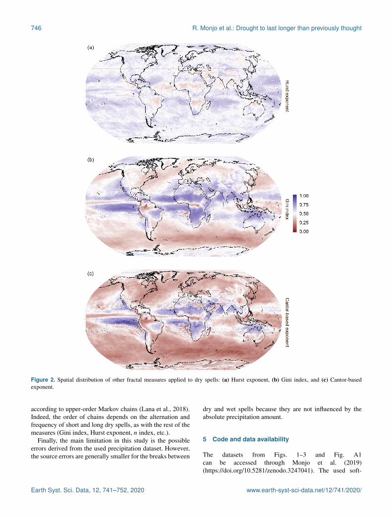
High values of the index (n > 0.4) are presented in thetropical and subtropical regions due to the effect of the sub-tropical anticyclones, particularly in the deserts. The savan-nah regions show the highest values of n, which involve along dry spell followed by shorter dry events. The polar re-gions score a secondary maximum of n due to the usuallylong but irregular dry events. Similar spatial results are foundif G and Ce are used (Fig. 2), while the Hurst exponent dis-plays noisier patterns around the world, very close to 0.5, asdescribed by other studies for Europe (Martínez et al., 2007;Lana et al., 2010). Most of the cases show values n < 0.5;similarly, approximately 80 % of theG values are lower than0.5. Both results indicate the existence of a noteworthy de-gree of homogeneity in the distribution of the dry spells alongthe time series. In fact, the Hurst exponent is close to 0.5 (i.e.the associated fractal dimension could be 1.5), which can beinterpreted as an equilibrium between positive and negativeautocorrelations.

3.2 Drought classification

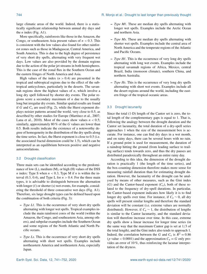
Three main sets can be identified according to the predomi-nance of low (L), medium (M), or high (H) values of the DSSn index: Type S when n < 0.3, Type M if n is within the in-terval (0.3, 0.4), and Type L for n > 0.4. For the three maintypes, it is advisable to distinguish between the alternationwith longer (`) or shorter (s) wet events, for example, consid-ering the threshold of three consecutive wet days (Fig. A1).Therefore, six large drought types can be defined based uponthe combination of both criteria (Fig. 3):

– Type L`. This is the occurrence of very short dry spellsalternating with longer wet spells. Tropical examples in-clude the main rainforest cores of the world (within theAmazon, the Congo, and southeastern Asia, among oth-ers), and subpolar examples include the Southern Oceanand some regions of the North Atlantic and North Pa-cific oceans.

– Type Ls. This is the occurrence of very short dry spellsalternating with short wet spells. Examples includenortheastern America and northeastern Asia, especiallyJapan.

– Type M`. These are median dry spells alternating withlonger wet spells. Examples include the Arctic Oceanand northern Asia.

– Type Ms. These are median dry spells alternating withshorter wet spells. Examples include the central area ofNorth America and the temperate regions of the Atlanticand Pacific Oceans.

– Type H`. This is the occurrence of very long dry spellsalternating with long wet events. Examples include thetropical savannah regions of Africa, Mexico, centralBrazil, India (monsoon climate), southern China, andnorthern Australia.

– Type Hs. This is the occurrence of very long dry spellsalternating with short wet events. Examples include allthe desert regions around the world, including the east-ern fringe of the tropical oceanic areas.

3.3 Drought lacunarity

Since the total (1-D) length of the Cantor set is zero, the to-tal length of the complementary gaps is equal to 1. That is,following the analogy between the drought duration and theCantor set lacunarity, the total duration of a dry-spell seriesapproaches 1 when the size of the measurement box is ac-curate. For instance, one can find dry days in a wet month,and on rainy days, there can be several hours with no rain.If a ground point is used for measurement, the duration ofa raindrop hitting the ground (from leading surface to trail-ing surface) tends towards zero, and thus the dry pauses aredistributed paradoxically throughout an entire rainy day.

According to this idea, the dimension of the drought du-ration is practically 1 (the length of the time series), andthe box-counting dimension therefore makes more sense formeasuring rainfall duration than for estimating drought du-ration. However, the lacunarity of the drought can be anal-ysed by means of other measures, such as the Gini index(G) and the Cantor-based exponent (Ce), both of these re-lated to the frequency of dry-spell durations. In particular,the Cantor-based exponent indicates how likely it is to findlonger dry spells over time. For instance, if Ce ∼ 0, all dryspells will present similar lengths and therefore the standarddeviation will be constant (i.e. extreme values are normallydistributed). However, if Ce ∼ 1, the distribution of lengthsis similar to the Cantor lacunarity, and the standard devia-tion will therefore increase over time. In this case, extremedry spells show a linear increase for longer time series (inthe same way that the maximum Cantor gap is set at 1/3 ofthe total length), and the Gini index also tends to approach 1.Indeed, the correlation between the G and Ce is R2

= 0.86(p value< 0.0001) and the approximation Ce =G only pro-vides an error of 10 %, thus reinforcing the lacunar interpre-tation of the dryness.

Earth Syst. Sci. Data, 12, 741–752, 2020 www.earth-syst-sci-data.net/12/741/2020/

R. Monjo et al.: Drought to last longer than previously thought 745

Figure 1. Spatial distribution of regularity of the lacunarity, averaging for all DSS events: (a) maximum expected dry spell (Y1) and (b) DSSn index.

4 Discussion

The DSS n index provides information on the structure ofdrought lacunarity, in particular measuring the probability ofregularity (if n∼ 0) or irregularity (if n∼ 1). Regular val-ues of dry spells indicate that similar dry-spell lengths areusually consecutive. Accordingly, irregular values imply thatlong dry spells are followed by much shorter dry sequences.It should be kept in mind a high degree of irregularity is cor-related with the longest dry spells (Fig. A3).

In short, the time patterns of the dryness of a climate canbe characterised in a simple manner by means of the n index.This indicator represents a synthetic DSS, computed by aver-aging all the DSS events of a considered time series. In eachDSS, a relative distribution can be observed of consecutivedry spells and the maximum dry-spell duration. For exam-ple, the highest values of the DSS n index (observed in partsof Africa) imply a high accumulation of dry-spell durationswith a low number of events considered, whereas the lowestvalues of the DSS n index (found in the northwestern Ama-zon) point to a constant and linear accumulation of dry spellspresenting the same (short) duration (Fig. A4).

The DSS n index therefore provides information on therelative distribution of dry spells, on the longest duration, andon the total accumulated duration. Indeed, the start and endof a synthetic DSS event can be established by the numberi of dry-spell events so that the averaged maximum durationYi is a particular threshold (e.g. 1 d, which is defined as thedry threshold of a DSS event). This idea enables the conceptof a DSS event to be employed as an alternative definition ofmeteorological drought, with diffuse borders that, paradoxi-cally, are well defined by the n index. For instance, if Yi = 0is considered to be drought borders, the total duration of thedryness coincides with the total length of a time series (as thelength of the supplementary gaps of the Cantor set). In thiscase, the difference between one drought and another is givenby the decay rate of the maximum dry spell (well measuredby the n index).

As in (fractal) wet spells, the behaviour of dryness is self-similar on all timescales – that is to say, dry spells can beused at the daily, monthly, yearly resolution, etc., consid-ering specific dryness thresholds. This is guaranteed by thegoodness of fit of the n index model (p value < 0.0001).The proposed mathematical definition is complementary tothe previous ideas on the persistence of dryness, for example,

www.earth-syst-sci-data.net/12/741/2020/ Earth Syst. Sci. Data, 12, 741–752, 2020

746 R. Monjo et al.: Drought to last longer than previously thought

Figure 2. Spatial distribution of other fractal measures applied to dry spells: (a) Hurst exponent, (b) Gini index, and (c) Cantor-basedexponent.

according to upper-order Markov chains (Lana et al., 2018).Indeed, the order of chains depends on the alternation andfrequency of short and long dry spells, as with the rest of themeasures (Gini index, Hurst exponent, n index, etc.).

Finally, the main limitation in this study is the possibleerrors derived from the used precipitation dataset. However,the source errors are generally smaller for the breaks between

dry and wet spells because they are not influenced by theabsolute precipitation amount.

5 Code and data availability

The datasets from Figs. 1–3 and Fig. A1can be accessed through Monjo et al. (2019)(https://doi.org/10.5281/zenodo.3247041). The used soft-

Earth Syst. Sci. Data, 12, 741–752, 2020 www.earth-syst-sci-data.net/12/741/2020/

R. Monjo et al.: Drought to last longer than previously thought 747

Figure 3. Climatic classification of meteorological droughts around the world: regions with low (L), medium (M), or high (H) values of theDSS n index, alternating with longer (`) or shorter (s) wet events.

ware code (R programming language) with a point examplecan be accessed through Monjo et al. (2019) at GitHub:https://github.com/robertmonjo/drought.

6 Conclusions

As a principal conclusion, the study demonstrates thatdrought lacunarity can be analysed with the use of self-similarity features obtained from the DSS n index. This mea-sure is useful for characterising the temporal and spatial pat-terns of drought, which are consistent with the climatic fea-tures established worldwide. For instance, localities present-ing very frequent wet spells alternating with short dry spellsprovide low values of the DSS n index (this is the case, forexample, in the Amazon, the Congo, and other rainforests).This results from an accumulation of isolated short dry spells,all presenting the same duration. Additionally, places withlonger dry spells (such as deserts) scored higher values onthe DSS n index. This result is logical because the n indexis strongly correlated with the maximum and average lengthsof dry spells as well as with the Gini index.

Consequently, we arrived at a second conclusion: themethodology developed can be used to classify typologies ofmeteorological drought. Indeed, six climate types have beenproposed: these result from the combination of three classesof DSS n index values (Type L when n < 0.3, Type H forn > 0.4, and Type M otherwise) and two sub-classes basedon the alternation with longer (`) or shorter (s) wet events.This classification could be useful with regard to monitoringpossible changes in drought patterns around the world withinthe context of climate change (Monjo et al., 2016; Craineet al., 2013; Madakumbura et al., 2019).

The third and most important outcome refers to the factthat consideration of dryness lacunarity provides a better un-derstanding of drought duration and helps to predict whendroughts start and finish. Further works may use other datasetat a global or regional scale (with more spatial resolution) toanalyse past and future climate change (e.g. by using CMIP6climate models). Moreover, future studies may focus on de-signing specific indicators to monitor hydrological and agri-cultural droughts, especially involving datasets on river dis-charges, soil moisture, water stress, or related damage. Inparticular, the value of the DSS n index is related to the effec-tive duration (according to borders determined by a thresholdof the minimum expected dry spell). Indeed, the best anal-ogy with regard to understanding the features of the DSS isCantor lacunarity; i.e. total dry spells are almost equal to thelength of the entire series (in the same manner that the totallength of Cantor voids is equal to 1). The methodology pre-sented here provides a set of potentialities: from analysingthe change of drought regimes to feeding indicators for mon-itoring impacts on agricultural or hydrological droughts, withthe possibility of using data with a higher spatial resolution.

www.earth-syst-sci-data.net/12/741/2020/ Earth Syst. Sci. Data, 12, 741–752, 2020

748 R. Monjo et al.: Drought to last longer than previously thought

Appendix A

Note that the mean dry spell (MDS) and the mean wet spell(MWS) are geographically distributed, with a strong corre-spondence between the high (low) values of the one and thelow (high) values of the other. A general zonal pattern is ob-served, albeit with a clear dissymmetry between the westernfacades of the continents and the eastern oceans, in tropical–subtropical latitudes, with high values of the MDS (low val-ues of the MWS), and their responses, with low (high) val-ues. The highest values of the MDS are concentrated inthe tropical–subtropical zones, especially in the Sahara andits continuation in the Arabian Desert, in the Persian Gulfand the waters of the Indian waters of the Indian Ocean, inlower California, in northern Chile, on the coast of Peru andits waters, in the Atlantic Ocean off the coast of Namibia,and towards the west–northwest of Australia (bordering withAntarctica). The most similar values between both indices,specifically with high values in both, are observed in theAsia-Pacific region (monzonic region), reflecting the divi-sion of the year into two halves, the rainy summer, with longrains, and the dry winter, with an absence of precipitation formany days in a row. This pattern can be detected in otherareas presenting a humid–dry tropical climate, such as thesouthernmost area of the Sahel, northeastern Brazil, an areain Africa (south of the Equator), and northern Australia. TheSW–NE diagonals of mid-latitudes with decreasing values ofthe MDS in the Atlantic and the Pacific are clearly appre-ciated, according to the westerlies and the track of the low-pressure systems.

For instance, let D = (2,1,10,4,8,10,20,1,2) be a timeseries of consecutive dry spells. A DSS event is built aroundthe minimum value (D0 = 1) as (10, 4, 8, 10, 20). Sub-sequently, maximum accumulated dry durations are Pi =(20,30,38,42,52), and the maximum averaged dry durationsare Yi = (20,15,12.7,10.5,10.4), which can be fitted overthe number of events (i) according to Eq. (3).

The fitted parameters for the first curve are k = 0.02811(3)and m= 0.4677(8) (R2

= 0.67, p value < 0.0001). Inthe second panel, the fitted curves are exponential (α1 =

0.997(3), β1 =−9.543(7), AIC ≈ BIC = 1.4× 106, R2=

0.91, p value < 0.0001), Gumbel (α2 = 1.225(3), β2 =

−10.01(1), AIC ≈ BIC =−1.2× 106, R2= 0.88, p value

< 0.0001), and opposite Gumbel (α3 = 3.829(2) and β3 =

−0.5347(9), AIC =−1.1× 106, R2= 0.87, p value <

0.0001), according to the Eqs. (6)–(8).Note that the minimum DSS n index corresponds to the

Amazon, where almost every DSS event lasts for only 1 d,and the accumulation of dry spells (Yi) is therefore very regu-lar. Furthermore, the maximum n index (close to the ZambeziRiver) represents an average DSS event with a maximumdry spell of 33 % of the total accumulated dry-spell length(most of the entire time series) and successive dry spells withshorter durations (as in the Cantor gaps).

Earth Syst. Sci. Data, 12, 741–752, 2020 www.earth-syst-sci-data.net/12/741/2020/

R. Monjo et al.: Drought to last longer than previously thought 749

Figure A1. Spatial distribution of mean dry spell (a) and mean wet spell (b) at a spatial resolution of 0.5◦× 0.5◦ according to the MSWEPdataset (1979–2016).

Figure A2. Method for defining DSS events and their corresponding n index.

www.earth-syst-sci-data.net/12/741/2020/ Earth Syst. Sci. Data, 12, 741–752, 2020

750 R. Monjo et al.: Drought to last longer than previously thought

Figure A3. Statistical relationship between (a) annual dry days (A) and the DSS n index and (b) maximum expected dry spell (Y1) and theDSS n index.

Figure A4. Fitted curves of DSS events (Eq. 4), according to the maximum accumulated dry-spell duration (Pi ) over the number of eventsconsidered (i), both normalised according to the total values.

Earth Syst. Sci. Data, 12, 741–752, 2020 www.earth-syst-sci-data.net/12/741/2020/

R. Monjo et al.: Drought to last longer than previously thought 751

Author contributions. The Cantor-based exponent and the n in-dex were designed by RM, and all the calculus and figures werecreated by DR, while RM and JMV interpreted the results and RMwrote the paper. All authors read and approved the final paper.

Competing interests. The authors declare that they have no con-flict of interest.

Acknowledgements. We are grateful for the support provided bythe RESCCUE project, which received funding from the EuropeanResearch Council under the European Union’s Horizon 2020 re-search and innovation programme (grant agreement no. 700174).We also wish to acknowledge the support received from the Span-ish projects CGL2017-83866-C3-2-R and Climatology Group 2017SGR 1362. We appreciate the interest in our research shown bythe Water Research Institute of the University of Barcelona and bythe Department of Algebra, Geometry and Topology of the Com-plutense University of Madrid.

Financial support. This research has been supported by the Eu-ropean Research Council (RESCCUE (grant no. 700174)) and theSpanish Ministry of Science, Innovation and Universities (grant no.CGL2017-83866-C3-2-R).

Review statement. This paper was edited by Alexander Gelfanand reviewed by Hasan Tatli and Serguei G. Dobrovolski.

References

Beck, H. E., van Dijk, A. I. J. M., Levizzani, V., Schellekens,J., Miralles, D. G., Martens, B., and de Roo, A.: MSWEP: 3-hourly 0.25◦ global gridded precipitation (1979–2015) by merg-ing gauge, satellite, and reanalysis data, Hydrol. Earth Syst. Sci.,21, 589–615, https://doi.org/10.5194/hess-21-589-2017, 2017.

Bezruchko, B. and Smirnov, D.: Extracting Knowledge FromTime Series: An Introduction to Nonlinear Empirical Modeling,Springer, 2010.

Boeing, G.: Visual analysis of nonlinear dynamical systems: chaos,fractals, self-similarity and the limits of prediction, Systems, 4,37, https://doi.org/10.3390/systems4040037, 2016.

Craine, J., Ocheltree, T., Nippert, J., Towne, E., Skibbe, A., Kembel,S., and Fargione, J.: Global diversity of drought tolerance andgrassland climate-change resilience, Nat. Clim. Change, 3, 63–67, 2013.

Crausbay, S. D., Ramirez, A. R., Carter, S. L., Cross, M. S., Hall,K. R., Bathke, D. J., Betancourt, J. L., Colt, S., Cravens, A. E.,Dalton, M. S., Dunham, J. B., Hay, L. E., Hayes, M. J., McEvoy,J., McNutt, C. A., Moritz, M. A., Nislow, K. H., Raheem, N., andTodd, S.: Defining ecological drought for the twenty-first cen-tury, B. Am. Meteorol. Soc., 98, 2543–2550, 2017.

Dayeen, F. and Hassan, M.: Multi-multifractality, dynamicscaling and neighbourhood statistics in weighted pla-nar stochastic lattice, Chaos Soliton. Fract., 91, 228–234,https://doi.org/10.1016/j.chaos.2016.06.006, 2016.

Feder, J.: Fractals, Plenum press, New York, Springer USA, 284pp., https://doi.org/10.1007/978-1-4899-2124-6, 1988.

Feng, D.-J., Rao, H., and Wang, Y.: Self-similar sub-sets of the Cantor set, Adv. Math., 281, 857–885,https://doi.org/10.1016/j.aim.2015.06.002, 2015.

Gaspard, P.: Chaos, Scattering and Statistical Mechanics, Cam-bridge University Press, 2005.

Hou, W., Yan, P.-C., Li, S.-P., Tu, G., and Hu, J.-G.: Appli-cation of long-range correlation and multi-fractal analysis forthe depiction of drought risk, Chinese Phys. B, B25, 019201,https://doi.org/10.1088/1674-1056/25/1/019201, 2016.

Imre, A. R. and Bogaert, J.: The Minkowski-Bouligand dimensionand the interior-to-edge ratio of habitats, Fractals, 14, 49–53,2006.

Kuznetsov, N. V.: The Lyapunov dimension and its estimation viathe Leonov method, Phys. Lett. A, A.380, 2142–2149, 2016.

Lana, X., Martínez, M. D., Serra, C., and Burgueño, A.:Complex behaviour and predictability of the European dryspell regimes, Nonlin. Processes Geophys., 17, 499–512,https://doi.org/10.5194/npg-17-499-2010, 2010.

Lana, X., Martínez, M., Burgueño, A., Serra, C., Martín-Vide, J.,and Gómez, L.: Spatial and temporal patterns of dry spell lengthsin the Iberian Peninsula for the second half of the twentieth cen-tury, Theor. Appl. Climatol., 91, 99–116, 2018.

Lucena, L. R. R. D., Júnior, S. F. A. X., Stosic, T., andStosic, B.: Lacunarity analysis of daily rainfall data in Per-nambuco, Brazil, Acta Scientiarum Technology, 40, E36655,https://doi.org/10.4025/actascitechnol.v40i4.36655, 2018.

López de la Franca Arema, N., Sanchez, E., Losada, T., Dominguez,M., Romera, R., and Gaertner, M.: Markovian characteristics ofdry spells over the Iberian Peninsula under present and futureconditions using ESCENA ensemble of regional climate models,Clim. Dynam., 45, 661–677, 2015.

Madakumbura, G. D., Kim, H., Utsumi, N., Shiogama, H., Fischer,E. M., Seland, O., Scinocca, J. F., Mitchell, D. M., Hirabayashi,Y., and Oki, T.: Event-to-event intensification of the hydrologiccycle from 1.5◦C to a 2◦C warmer world, Sci. Rep., 9, 3483,https://doi.org/10.1038/s41598-019-39936-2, 2019.

Mandelbrot, B.: How long is the coast of Britain? Statistical self-similarity and fractional dimension, Science, 156, 636–638,1967.

Mandelbrot, B.: Self-affinity and fractal dimension, Phys. Scripta,32, 257–260, 1985.

Martín-Vide, J. and Gomez, L.: Regionalization of Peninsular Spainbased on the length of dry spells, Int. J. Climatol., 19, 537–555,1999.

Martínez, M. D., Lana, X., Burgueño, A., and Serra, C.: Lacunarity,predictability and predictive instability of the daily pluviometricregime in the Iberian Peninsula, Nonlin. Processes Geophys., 14,109–121, https://doi.org/10.5194/npg-14-109-2007, 2007.

Meseguer-Ruiz, A., Olcina, J., Sarricolea, P., and Martin-Vide, J.:The temporal fractality of precipitation in mainland Spain andthe Balearic Islands and its relation to other precipitation vari-ability indices, Int. J. Climatol., 37, 849–860, 2017.

Monjo, R.: Measure of rainfall time structure using the dimension-less n-index, Clim. Res., 67, 71–86, 2016.

Monjo, R. and Martin-Vide, J.: Daily precipitation concentrationaround the world according to several indices, Int. J. Climatol.,36, 3828–3838, 2016.

www.earth-syst-sci-data.net/12/741/2020/ Earth Syst. Sci. Data, 12, 741–752, 2020

752 R. Monjo et al.: Drought to last longer than previously thought

Monjo, R., Gaitán, E., Pórtoles, J., Ribalaygua, J., and Torres, L.:Changes in extreme precipitation over Spain using statisticaldownscaling of CMIP5 projections, Int. J. Climatol., 36, 757–769, 2016.

Monjo, R., Royé, D., and Martin-Vide, J.: Drought lacunarityaround the world and its classification (Version v0.1) [Data set],Zenodo, https://doi.org/10.5281/zenodo.3247041, 2019.

Olsson, J., Niemczynowicz, J., Berndtsson, R., and Larson, M.: Ananalysis of the rainfall time structure by box counting—somepractical implications, J. Hydrol., 137, 261–277, 1992.

Plotnick, R. E., Gardner, R. H., Hargrove, W., Prestegaard, K., andPerlmutter, M.: Lacunarity analysis: A general technique for theanalysis of spatial patterns, Phys. Rev. E, 53, 5461–5468, 1996.

Sakhr, J. and Nieminen, J. M.: Local box-counting dimensionsof discrete quantum eigenvalue spectra: Analytical connectionto quantum spectral statistics, Phys. Rev. E, E97, 030202,https://doi.org/10.1103/PhysRevE.97.030202, 2018.

Sen, Z.: Wadi Hydrology, CRC Press, 368 pp., 2008.Tatli, H.: Detecting persistence of meteorological drought via the

Hurst exponent, Meteorol. Appl., 22, 763–769, 2015.

Vicente-Serrano, S., Van der Schrier, G., Beguería, S., Azorin-Molina, C., and Lopez-Moreno, J.: Contribution of precipitationand reference evapotranspiration to drought indices under differ-ent climates, J. Hydrol., 426, 42–54, 2015.

Vicente-Serrano, S. M., Beguería, S., and López-Moreno, J.: AMulti-scalar drought index sensitive to global warming: TheStandardized Precipitation Evapotranspiration Index – SPEI, J.Climate, 23, 1696–1718, 2010.

Wilhite, D. and Glantz, M.: Understanding the Drought Phe-nomenon: The Role of Definitions, Water Int., 10, 111–120,1985.

Wilkinson, M., Pradas, M., Huber, G., and A., P.: Lacu-narity exponents, J. Phys. A-Math. Theor., 52, 115101,https://doi.org/10.1088/1751-8121/ab0349, 2019.

Yu, S., Piao, X., Hong, J., and Park, N.: Bloch-like waves inrandom-walk potentials based on supersymmetry, Nat. Com-mun., 6, 8269, https://doi.org/10.1038/ncomms9269, 2015.

Earth Syst. Sci. Data, 12, 741–752, 2020 www.earth-syst-sci-data.net/12/741/2020/