Meteorological and source analysis of smog events during ...

I

_._... ________ -nnav,."""-•---

THc_ 1 ,-: 1 1 - J DE T OF-CJ. i · 1 -llt\--r,o:--J & I A D M. NAGEMENT

1 2 AU6 1997 11.'ESTERN AUSTRALiA

Meteorological and source analysis of smog events during the Perth Photochemical Smog Study

Dr Peter Rye

Department of Environmental Protection Perth, Western Australia

Technical Series 83 May 1996

..

ISBN. 0 7309 5784 5 ISSN. 1030 -0600

Contents

Page

1. Introduction ....................................................................................................................................................................................................................................... 1

2. General Meteorology of Smog Events ........................................................................................................................................................ 2

3. Summer Conditions, 1992-1995 .......................................................................................................................................................................... 4

4. Classification of Photochemical Smog Events ............................................................... 5

5. Summary of Smog Events, 1992-1995 ........................................................................................................................................................ 6

5.1. 22 October 1992 ....................................................................................................... 7

5.2. 5 December 1992 ..................................................................................................... 8

5.3. 6 December 1992 ................................................................................................... 11

5.4. 12 December 1992 ................................................................................................. 12

5.5. 5-7 January 1993 .................................................................................................... 13

5.6. 8 January 1993 ....................................................................................................... 14

5.7. 13 January 1993 ..................................................................................................... 17

5.8. 9 February 1993 ..................................................................................................... 18

5.9. 12 February 1993 ................................................................................................... 19

5.10. 17 February 1993 ................................................................................................... 21

5.11 16 December 1993 ................... : ............................................................................. 22

5.12. 22 January 1994 ..................................................................................................... 24

5.14. 23 January 1994 ..................................................................................................... 25

5.14. 31 January 1994 ..................................................................................................... 25

5.15. 4 February 1994 ..................................................................................................... 27

5.16. 19 February 1994 ................................................................................................... 30

5.17. 3 March 1994 ......................................................................................................... 34

5.18. 4 March 1994 ......................................................................................................... 35

5.19. 8 March 1994 ......................................................................................................... 36

5.20. 12 March 1994 ....................................................................................................... 37

5.21. 16 March 1994 ....................................................................................................... 39

5.22. 17 March 1994 ..................................................... .-................................................. 40

5.23. 18 March 1994 ....................................................................................................... 41

5.24. 21 March 1994 ....................................................................................................... 43

5.25. 14 April 1994 ......................................................................................................... 44

5.26. 16 December 1994 ................................................................................................. 45

5.27. 17 December 1994 ................................................................................................. 46

5.28. 16 January 1995 ..................................................................................................... 47

5.29. 17 January 1995 ..................................................................................................... 48

5.30. 18 January 1995 ..................................................................................................... 49

5.31. 31 January 1995 ..................................................................................................... 50

5.32. 10 February 1995 ................................................................................................... 50

5.33. 12 February 1995 ................................................................................................... 51

5.34.· 17 February 1995 ................................................................................................... 52

5.35. 20 February 1995 ................................................................................................... 53

5.36. 21 February 1995 ................................................................................................... 53

5.37. 22 March 1995 ....................................................................................................... 55

6. Sea Breeze Front Movement on Potential Smog Days ................................................ 56

7. Conclusions ................................................................................................................... 57

8. References ..................................................................................................................... 58

1. Introduction In 1989 the WA Department of Environmental Protection established an air quality monitoring station at Caversham (See figure 1). The purpose of this station was to measure concentrations of ozone and nitrogen oxides downwind of the city, in conditions with potential to generate photochemical smog.

Measured hourly averages of ozone in excess of 80 ppb (Canadian / WHO acceptable limit) indicated that Perth was experiencing at least the beginnings of photochemical smog. The Perth Photochemical Smog Study was subsequently undertaken by Western Power and the Department of Environmental Protection, to provide a detailed understanding of the occurrence of smog events, over the whole of the Perth region.

1''' Quinns Rocks iS]

~ Rottnest Island

N • o--; 1t"Ts

0Gingin

•Pinjar

KEY D DEP monitoring sites 0 PPSS monitoring sites /j. Bureau of Meteorology sites • Meteorology-only sites

Figure 1. Measurement sites used in the Perth Photochemical Smog Study.

The major components of the study included the continuous monitoring of photochemical smog species (at Caversham, and shaded sites in figure 1) and of meteorological variables, the development of an emissions inventory, and adaptation of existing computer models to represent the transport and photochemistry of smog in the region. In addition, a major field measurement exercise was conducted through the summer of 1993-1994, with the aim of characterising in detail a number of photochemical smog events.

All measurements quoted in this report were logged as ten-minute averages. Hourly values were calculated from these measurements, with the highest found from running averages, rather than averaging within each clock hour.

The continuous monitoring programme showed that the Perth metropolitan area experiences about ten days each year when the concentration of ozone within photochemical smog exceeds 80 ppb. Over the period 1989-1995, when measurements have been available from Caversham, there has been no significant trend in this frequency. The highest hourly average

1

each summer (apart from the partial summer record of 1989-1990) has always exceeded 100 ppb, the highest measured being 133 ppb.

The purpose of this report is to provide a day-by-day summary of the smog events during the PPSS period, and of their related meteorology. It should provide a basis for further modelling and data analysis arising from issues raised by the study.

2. General Meteorology of Smog Events The only periods in the Perth region when ozone concentrations rise significantly above background involve the inland advance of the sea breeze. Peak ozone concentrations occur just after the passage of the sea breeze front. The highest concentrations are measured when a morning easterly wind carries urban emissions offshore, and a south westerly sea breeze develops and brings the reacting air mass back over the city.

Figure 2 shows measurements made at Caversham on 18th January 1991, on the day of one of the highest ozone concentrations so far measured. The ozone peak between 14 and 15 hours (2pm to 3pm) was at a typical time of day. The arrival of the sea breeze can be seen in a wind direction change through 180° and a speed increase, at about 2pm Ozone concentrations rose shortly after the first wind direction change, and immediately after the speed increase. This pattern is normal at inland sites in the Perth region.

Speed 9

(m/s) 6 ...... .

3

12 4 Time (hours WST)

Figure 2. Time sequences of (top to bottom) ozone concentration, wind direction and wind speed, measured at Caversham on 18 January 1991.

Apart from the sea breeze, there is another contributing phenomenon, known as the west coast trough. Its formation relates both to the sea breeze, and the region's normal summer weather cycle.

This cycle involves a period, of length roughly one week, over which synoptic-scale high pressure systems pass south of the state. Winds change from south easterly, through to north easterly, then briefly through to the south west before returning to south easterly again.

2

Sea breezes develop on most days of the cycle. Due to the slow overnight cooling of the land, and the low friction of the ocean surface, the offshore component of the sea breeze flow can persist overnight. The persisting southerly component means that, due to the requirement of geostrophic balance, an onshore pressure gradient develops. As inland winds turn to north easterly, a significant low pressure trough can develop offshore (e.g., Figure 3).

Figure 3. The coastal low pressure trough on the morning of 16 March 1994 was a typical example of this feature. Pressures shown are in hPa (hectopascal).

The coastal trough has several implications for the occurrence of smog events in the Perth region.

• Light winds near the trough axis ensure that any morning pollutant emissions from the city do not travel far offshore.

• The existence offshore of a southerly flow (with a small westerly component due to friction) eliminates any chance of the escape of pollutants westward.

• Due to the southerly component to the west of the trough axis, air temperatures in this region are much cooler than those to the east of the trough. This means that, when the trough finally moves inland, atmospheric stability neeµ- the surface is high, and mixing depths are reduced.

When these conditions are not met (for example, when the morning easterly is stronger) urban emissions can escape from the returning sea breeze flow, keeping smog concentrations low.

3

3. Summer Conditions, 1992-1995 The 1992-1993 summer began with fairly cool temperatures. The long-term daily average for December at Perth Airport is 22°c, and most days at Caversham were below this (Figure 4). Brief warm periods are the norm for December, and longer periods of high temperatures did not commence until about a week into January. However, in December's brief hot spells, three significant smog events occurred.

Temperatures were close to average in January and February, but fell below the March average early in that month, and remained so. This ensured that no smog events occurred after the end of February.

The summer of 1993-1994 was a mixture of unusual patterns, although the total effect was close to average. December was characterised by large excursions of temperature about the mean. During a hot spell over 16-17 December (See section 5.11), a smog event occurred, although windy conditions kept ozone concentrations moderate. Early in January, a regime of south westerly winds resulted in no photochemical smog events. Later in the month, strong high pressure systems to the south east of the state allowed strong coastal troughs to form. As in the December case, these were found to bring conditions generally too windy for the occurrence of high ozone concentrations. The sole exceptions were two events caused by bushfire smoke, summarised in sections 5 .12 and 5 .13.

Windy and mild conditions persisted - with exceptions - through the PPSS intensive study period of early February. Not until late February were there any good examples of the moderate north easterly / coastal trough conditions normally associated with smog formation. From this time onward conditions remained warm, and moderate to high smog levels occurred on several occasions. Figure 4 shows, in particular, that temperatures in the first three weeks of March remained well above average. A sequence of smog events to 21 March (See sections 5.21 to 5.24) marked the effective end of the summer season.

35...-----------------------------

Temp. 25+-<• •~HIH'r-l-V.il---l~H-1~,~~

20

r:•'-'""""''"''"" 1992-1993 15 --------------------1993-1994

--1994-1995

10+----+---+----+----+------i,-----+----1-----1

1-Dec 16-Dec 31-Dec 15-Jan 30-Jan 14-Feb 1-Mar 16-Mar 31-Mar

Figure 4. Daily average temperature at Caversham for the three summer seasons of the study. Monthly average temperatures for Perth Airport are shown as

horizantal lines.

4

The temperatures through the summer of 1994-1995 were generally warmer than those of the preceding two summers. Temperatures in December were usually above average, although conditions were suitable for smog formation from urban emissions on only one day (See section 5.26). The pattern persisted in early January, with above average temperatures but no significant smog episodes. From then to the end of the month the daily average temperature fell, although remaining above the long-term average. The change also coincided with conditions more favourable for smog development, with five events from 16 to 31 January (sections 5.28 to 5.31).

After a cool start, two hot periods occurred in February, both including days of significant smog events. March was again warm, temperatures being similar those of March 1994, but only a single smog event occurred (See section 5.37).

The experience of the three summers of the study has indicated that December tends to be too cool and, when not too cool, too windy for major smog cases. January tends to be warmer, but can also be windy, so smog events do not occur with any regularity. From late January into March, periods of lighter winds permit more common smog episodes. The end of the time of the year when smog events can occur is determined mainly by end of summer temperatures, at some time in March.

4. Classification of Photochemical Smog Events Although photochemical smog occurs within a restricted set of conditions in Perth, variations have been found in the mix of responsible sources, and the progress to completion of the smog reactions. These are likely to have implications for future management techniques.

Over the full sample of smog events for the last three summers, there were three identifiable classes (two of which were very similar) giving rise to the highest ozone concentrations, and a few others that were sufficiently different to these to justify separate grouping. The major classes were:

1. Inland Events: Days on which ozone concentrations inland were significantly greater than at the coast, consistent with further progress of smog chemistry as the air mass moved inland. These conditions are those leading to the form of smog episode originally detected at the Caversham monitoring site. The meteorology of the day normally involves a cool inflow, with low mixing depths persisting inland. The case on 4 February 1994 (section 5. 15) was close to typical of this regime, except for cooler than ,normal temperatures.

2. K winana Events: These are identified when trajectories to inland sites lead back to the Kwinana region, as well as passing across the city or suburbs. Coastal sites may also receive high ozone levels, sometimes due solely to emissions from the Kwinana region. These cases show more southerly winds, otherwise a meteorological regime similar to the "inland" class. The case on 8 January 1993 (section 5.6)_was a good example.

3. Coastal Events: These are characterised by highest concentrations at the coast. Most commonly, the meteorological regime comprises a fresh easterly gradient wind, followed by passage inland of the coastal trough or sea breeze. The decreased concentrations inland are probably the combined result of dilution as mixing depth increases, along with the late arrival of smog at the coast, so that the smog-producing chemical reactions were already close to completion. The most extreme example of this class occurred on 19 February 1994 (section 5.16).

5

The following minor classes were also identified. These generally gave lower ozone concentrations, or were otherwise less useable for detailed study.

4. Stalled Sea Breeze Events: These develop when the inland edge of the sea breeze does not penetrate completely across the coastal plain. As for coastal events, with which they share some characteristics, these result in lower ozone concentrations inland, due to the failure of the smog front to reach inland sites. A good example of this class occurred on 20 February 1995 (See section 5.35).

5. Strong Trough Events: When broad masses of ozone of moderate concentration passed across the city, associated with the movement inland of a strong coastal trough. In comparison to the "coastal event" class, these were characterised by stronger morning winds. Ozone concentrations are fairly uniform across the metropolitan area. The smog event on 16 December 1993 (section 5.11) was a representative example.

6. Bushfire Smoke Events: These occur when smoke from controlled bums or other bushfires is brought across the urban area in daytime. The smoke includes highly reactive VOC's, and experience has shown that their reaction with urban emissions generates ozone concentrations similar to those generated by urban emissions alone. The significant difference is that these events can occur in periods of persisting south westerly winds, when smog levels would normally be low.

While their impact is high, inclusion of these events in a predictive analysis is difficult, because of the essentially unknown photochemical reactivity of the smoke. A clear example occurred on 13 January 1993 (See section 5.7).

7. Light Westerly Wind Events: These were relatively rare, occurring when low mixing depths and light morning winds allowed accumulation of overnight and morning emissions. Ozone formed as the air mass moved slowly inland, on a light westerly or south westerly wind. See section 5.19, which summarises an example of this class that occurred on 8 March 1994.

The following section presents daily summaries, for the full period of the study, in date sequence, covering each of these classes.

5. Summary of Smog Events, 1992-1995 Before the study, the Caversham site was the sole source of understanding of Perth's photochemical smog climate. One role of the extended monitoring network was to develop a more detailed knowledge of the frequency of occurrence and distribution of smog events in the region. The details below summarise the most significant smog events that occurred during the period of the study.

The criteria used to define "significant" are subjective. The events described below include all those for which ozone concentrations at some site exceeded 80 ppb, but others important because of the sources or meteorology involved are also included.

For each day, a figure summarising the highest hourly average ozone concentrations, across the monitoring network, is shown. There is a black unshaded rectangular box for each site, which corresponds to the reference standard of 80 ppb, and a shaded box whose height represents the peak hourly average ozone value. For simplicity, these are not given figure references.

6

5.1. 22 October 1992 This was unusually early in the season, and developed due to the passage over the city of a major mass of bushfire smoke.

Controlled burns on the previous day, in the 1 region to the north east of the city, appear to [

1

,,

have been responsible. High haze levels at Queens Buildings and Hope Valley overnight JOuinns Rocks

from 21-22 October (figure 5) showed that the . smoke moved coastward, and offshore. There lswanbourne was a weak low pressure trough located just :,I ~ offshore. It appeared that urban emissions : which crossed the coast in the morning mixed 1

with smoke, and the concentrations of ozone were already high when the air mass arrived at the coast at Swanbourne (figure 6). A more ' detailed analysis of this event was given by Rye (1995).

Caversham A.Q.M.S.

Visibility 6

(Bsp)

Visibility (Bsp)

,,,~

12 18

Queens Buildings A.Q.M.S.

18

Hope Valley A.0.M.S.

12 18

8 October 1992

Kenwick

24

24

24

Figure 5. Light backscatter (haze) measurements made at Caversham, Queens Buildings and Hope Valley on 22 October 1992. Vertical axis measurements are

in units of I o-4 m-1. _

7

15~ 12

Ozone 90 (ppb) 60

06

Caversham A.0.M.S.

12 24 Swanbourne A.O.M.S.

30

00 1sq 12d ~~~i)to~

0oc,o"""==· ===-o.,.6~~===~12=====::..;.:.,..1s=====~24

Figure 6. Ozone concentration time sequences at Swanboume and Caversham on 22 October 1992.

5.2. 5 December 1992 The sea breeze developed slowly on this day, replacing a morning easterly wind. Swanbourne was the only location at which 80 ppb was reached, but concentrations here built up slowly through the day. The sea breeze did not bring increased ozone concentrations to inland sites until about 4pm.

A trajectory calculation (figure 7) indicated recirculation of urban emissions along a long path. Trajectories to Cullacabardee and Caversham were similar to the shown trajectory, to Swanbourne, but with extension inland.

The high temperature at Swanbourne (figure 8) was typical of a coastal event, but the ozone measurements at inland sites (figure 9) and air mass trajectories pointed to contributions from

5 December 1992

i . . Cull<6abardee

Cavers ham

Qi]"~\'' ::i Kenwick

both urban and Kwinana emissions. Double peaks occurred at Kenwick, Caversham and Cullacabardee, with early ozone being clearly due to returned urban emissions. The later, smaller peak probably represented the effect of later, more southerly winds, bringing Kwinana emissions to the metropolitan area.

8

\/ \ ( ', \ ~-\

\

\ ~\

Figure 7. Air mass trajectory ending at Swanboume at 4:30pm on 5 December 1992. The numbers on the trajectory are times in hours WST.

Ozone

(ppb)

(deg.C)

270 Direction

180 (deg.)

90

0 06 12 18

Figure 8. Ozone, air temperature and wind direction measurements at Swanboume on 5 December 1992.

9

4

4

4

120 .. K~.rnyic::f<:Ac9.,M,.$._ . 100 ................ _______ _ ----- --···-·-----···-·-~·•--·-----

Ozone 80 --------------------------(ppb) 60 +------------------~

40t::=:::;:;::;:;::::::=:;;;;=:::::::::::::::=;;;tn~hJ0 20 I,,'.'

0

120 . 100 ·················-·····--·· ........ -................. _____ ----80

Ozone 60 (ppb) 40 20

120.------------------------------1001---------------------------80 +---------------------------

Ozone 60 (ppb) ------------------"'

Figure 9. Ozane measurements at three inland sites on 5 December 1992. A double peak is evident in all cases.

10

5.3. 6 December 1992 Ozone concentrations were relatively lower than other days reviewed. The event was classified as "stalled sea breeze". Although the sea breeze arrived 1330-1400, its front remained close to the coastline. Levels at Caversham and Kenwick rose only a little above background, as a result.

Figures 10 shows trajectories to Swanboume and Quinns Rocks ending at 1500 and 1800 WST (the time limits of the ozone event). These suggested that urban emissions were the dominant source of the measured ozone.

lswanbourne

(;;J Ill

6 December 1992

Cull0cabardee

0~ fddfJ 'ij1~1l:;:£

Cavers ham

Kenwick

Figure 10. Calculated air mass trajectories to Swanbourne (right) and Quinns Rocks (left) over the periods of highest measured ozone concentrations, on 6

December 1992.

11

5.4. 12 December 1992 This day was significant because it followed a pattern expected later in the summer season. The coastal trough was located close to the coastline in morning, with very light southerly winds at coastal sites, and a stronger southerly at Rottnest.

Trajectories ending at Caversham during the period of the smog event (12:30 to 2:30pm) generally pointed out into the coastal trough region, south of Rottnest. There were some indications of a Kwinana contribution to the early part of the period.

Quinns Rocks

Swanbourne Ii ,,·,;

~

12 December 1992

Ii Ill Cullacabardee

0

I 0 .

Caversham

Ozone concentrations on the coast, at Kenwick

Swanbourne, were close to 40 ppb for the period 9am to 3pm, with very little NO or NO2 present. This is consistent with the inflow air having remained in the trough for a long period, rather than coming recently from the Kwinana region. It also shows that inland concentrations were due to the reaction of the day's urban emissions, with a low mixing depth probable.

The day followed the pattern of an "inland event" (figure 11). There may have been a contribution from the previous day's urban emissions. However, with back trajectories all extending southward, the likely source of the smog brought in by the trough was either Kwinana, or bushfire smoke.

150 ---------------------------------

120 ____ ._ ............................. ,---···· ...... ,. ...... ,. ........................................ ,

Figure 11. Ozane concentration (ppb) at Caversham on 12 December 1992.

12

5.5. 5-7 January 1993

5 January 1993

Qu;nn's Rocks Culla-rdee Rolling Grtl o 0 Ii Swa bourne

Rottnest Iii ,,e;;:,

Kenwick

These three days were of similar nature, and occurred during the initial sonde team exercises of the study. Highest ozone concentrations were measured at Quinns Rocks, with the sea breeze front stalled slightly inland on the 5th, advancing only slowly on the 6th and 7th. Morning winds were E-ENE on the 5th, ENENE on the 6th, lighter NE on the 7th.

Trajectories showed Quinns Rocks received a general spread of urban emissions on all days Figure 12 shows trajectories for January 6. There was a long period of elevated ozone levels at Swanbourne, with small peaks of ozone at 3pm at Caversham and Cullacabardee.

The days all represented the "coastal event" pattern.

13

6 January 1993

i) .

7 January 1993

Two Rocks

Quinns Rocks

I Swa

Rot est I ,,e;;:,

Kenwick

Figure 12. Trajectories ending at Quinns Rocks at 1, 2 and 3pm on the 6th January 1993.

5.6. 8 January 1993 Ozone concentrations on this day included the highest measured inland during PPSS.

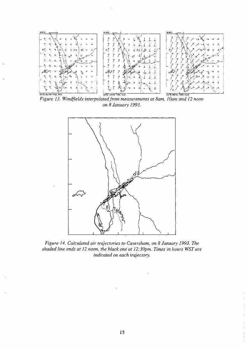
The trough was just offshore in morning, as shown by the southerly winds at Rottnest island (figure 13).

Trajectories ending at Caversham at 12 noon to 12:30pm, when high ozone levels commenced, passed Kwinana during a morning period of light winds (figure 14). However, trajectories ending at the time of when ozone concentrations at Quinns Rocks and Two Rocks were rising (10:30 and 9:30am respectively) originated late on the previous evening, at Kwinana. These features indicated that, while the highest ozone concentrations were due to emissions on the day, the pattern for this case was close to that of a "multi-day" smog event.

I .

.

.

.

Quinns Rocks

Rottnest

~

Cullacabardee

8 January 1993

Rolling Grieen

0 .

.

Cavers ham

Kenwick

Figure 15 presents time sequences of some measurements made at Caversham on this day. The close coincidence of the rise of sea breeze wind speed and ozone concentrations, very evident in the figure, is typical. Lighter westerlies before this time represented air trajectories which did not come from offshore.

14

10 MIS: ~ ,oMJS: ~

DATE: 080193 TIME: OB:00 DATE: 080193 TIME: 10:00 DATE: 080193 TIME: 12:00

Figure 13. Windfields interpolated from measurements at 8am, 1 Oam and 12 noon on 8 January 1993.

Figure 14. Calculated air trajectories to Caversham, on 8 January 1993. The shaded line ends at 12 noon, the black one at 12:30pm. Times in hours WST are

indicated on each trajectory.

15

120 ························································ 100 >•••••••••••••••••••••••••••••••••m••---

80 ----------------------------····-----··· N02 60 +-----------------------------

(ppb) 40 1-------------------------_::

120 100--------------------------

NO 80 +----------------------------

(ppb) 60 40 ~~---------------------------20 o J~E~tfL..L:!i.L-:::i::-~------~

1 :------:::::.:::::;~---:::::::.::::::::=....e:...-:d.

120-r----------100 80

Ozone 60 +--------------

(ppb) 40 t------------;::::;:::;_;:_;:Ji·cycr;;;;;;; ;c. ·"-.-._-_...--=._-__,.--;;;,.:--_-------20 o o·-1:c,-----1.____..;:...;::;.:;....u;,,,,;;;;.....~~=--~~......,.,..;.;:.;;.;.=--=--.......;-.;.;:.;;.;...,.:,,,.----..;;;;.;:;.--::;..;:,.~.,,.i

5...--------------

4

Visibility 3-t----------------------------

(Bsp)

1 ... ·- ....

360

Wind 270

Dir. 180 (Deg.)

90

0

12

Wind 9

Speed 6 (mis)

3

0

Figure 15. Time sequences of ozane, nitrogen oxides, visibility (measured by nephelometer), wind speed and wind direction at Caversham on 8 January 1993.

16

2

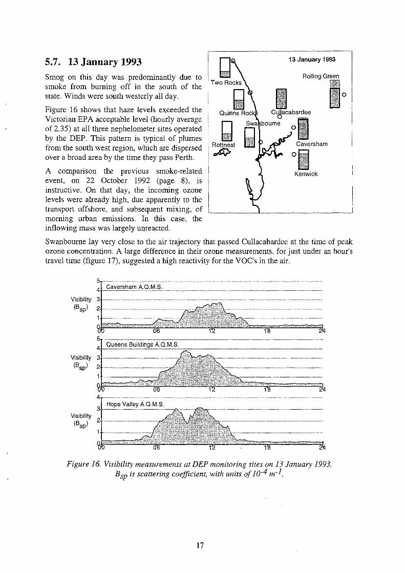
5.7. 13 January 1993 Smog on this day was predominantly due to smoke from burning off in the south of the state. Winds were south westerly all day.

Figure 16 shows that haze levels exceeded the Victorian EPA acceptable level (hourly average of 2.35) at all three nephelometer sites operated by the DEP. This pattern is typical of plumes from the south west region, which are dispersed over a broad area by the time they pass Perth.

A comparison the previous smoke-related event, on 22 October 1992 (page 8), is instructive. On that day, the incoming ozone levels were already high, due apparently to the transport offshore, and subsequent mixing, of morning urban emissions. In this case, the inflowing mass was largely unreacted.

13 January 1993

Rolling Green

0

Swanbourne lay very close to the air trajectory that passed Cullacabardee at the time of peak ozone concentration. A large difference in their ozone measurements, for just under an hour's travel time (figure 17), suggested a high reactivity for the VOC's in the air.

Visibility (Bsp)

Visibility (Bsp)

5

4 Caversham A.Q.M.S.

3

2

1

~ 5

Queens Buildings A.Q.M.S.

4 ................................ .

3 Hope Valley A.Q.M.S.

Visibility (Bsp) 2 ........................... _

18 2

2

2

Figure 16. Visibility measurements at DEP monitoring sites on 13 January 1993. Bsp is scattering coefficient, with units of 10-4 m-1.

17

120 100 .... swanbourneA.Q.M.S.

Ozone 80

(ppb) 60 ----------------··················--·-···------40 20

2

100 Cullacabardee A.Q.M_.S_. _____ _

Ozone 80 t------------------------------(ppb) 60 +------

40 +------------c,~•· 20 ~---------/ 0 n~===~..:..::::~:.:.,:;_;;.;;;;_;:~~~~~~~~~~-=:::::::::,. ___ ~2'

120 100 Caversham A.Q.M.S.

80 Ozone 60 (ppb)

40 20 ····-·-·----··---··

0 0 2

Figure 17. Ozone concentrations at two inland sites ( Caversham and Cullacabardee) and a coastal site (Swanboume) on 13 January 1993. The high

reactivity of the incoming smoke is evident as a large change of ozone concentration between the sites.

5.8. 9 February 1993 This day showed features characteristic of a range of types of smog event. The sea breeze arrived at the coast about noon. Trajectories (see figure 18) indicated Quinns Rocks and Two Rocks received late morning urban emissions, while Caversham and Cullacabardee received the K winana plume. Concentrations were highest at Quinns Rocks, but values at Cullacabardee, Caversham and Kenwick were higher than normal for a coastal event.

18

9 February 1993

Rottnest

~

Kenwick

4

/' 3

_;

~-;

3 • : /._,,,.,,.----/

J_,/ 12

Figure 18. Calculated air trajectories ending at Two Rocks, Quinns Rocks, Cullacabardee and Caversham at the times of the peak ozone concentrations at

each site, on 9 February 1993.

5.9. 12 February 1993 The highest ozone concentrations at Rottnest Island, for the 1992-1993 summer, were experienced on this day.

All coastal sites appeared to have received a double peak (Figure 19). The first (larger) was evidently due to urban emissions, the second came from further south.

Accurate back-trajectory calculations for the times after 3pm (including the second peaks) were not possible, because trajectories extended west of Rottnest, the limit of wind measurements. However, due to the presence of a trough offshore, with more southerly wind components, any calculated back trajectory could be expected to be displaced southward. The northern limiting source regions were the

I . . 12 February 1993

Cullac[5dee

• 0

II Swa~b urne

I . Rottnest Caversham ~ oi

Kenwick

northern edge of the Kwinana industrial area for the Swanbourne site, and the southern suburbs for Rottnest and Quinns Rocks. The implied source region was therefore the Kwinana industrial area.

Rolling Green experienced higher concentrations than other inland sites. Figure 20 shows the probable cause was the double passage over the Perth region of the air that reached this site at the time of the ozone peak.

19

120 .................................. . 100 ,.__0-'--ui_nn_s_R_o _____ c ___ ks .............. Ac...:.Q.:.:...M'--'--=.S-'-. _________________ _

801-----------------=-~-------0zone

60 ,_ __ _

(ppb) 40 1---------------,.-,-,

201-----:::::====:::::;::::::;::::::?5't'~~r: 0Ai-r---====~=====~.p;;-====---::11x-=====-',,i 120 ~------------------------100 _§_w_a_n_b_ou_~~.~~.9:r-.,i:s.

ao----------------------------Ozone 60 +--------------~,..✓,

(ppb) 40 ···

2~r~==:~=====~;;;;;:~~1,~····~,~,~ 4

120 r--------------------------Rottnest Island A.Q.M.S. 100+---------------------------

80+----------------.l'S§',---------Ozone 60 +--------------c

(ppb) 40

20r-,,.....~--.,.,...,.....,..,-,.-.,.,.....,...,.....~. oAi-r-------~----------~.p;;-----'--'--~~--------'---,l4

Figure 19. Ozane concentrations at the three coastal measurement sites, on 12 February 1993. The data gapfor the Rottnest Island sequence was due to the

instrument's being out of operation for a short period. The dotted line indicates the probable trend through this period.

Figure 20. Calculated air trajectory ending at Rolling Green at 4:30pm on 12 February 1993, the time of the day's peak ozane concentration at the site.

20

5.10. 17 February 1993

The coastal trough was close to the shoreline in the morning. The day appeared at first a traditional "inland event", but potentially also involved the previous day's emissions.

Analysis of trajectories ending at Cullacabardee and Caversham at the time of maximum smog potential showed that the Kwinana industrial area was probably a major contributor to the smog event (Figure 21a). However, with an overnight north easterly wind, calculations were extended to the previous day. These (Figure 21 b) suggested that the evening erruss1ons from the Perth region, for the previous day, had also contributed.

A check of the NO and N02 concentrations at the Hope Valley site, between 7 and 8am on

T jlL,, 17 February 1993

Ji Ro ks culbardee Romng I:

Kenw1ck

17 February, showed totals ranging from 4 to 8 ppb. These were higher than normal for the wind direction, supporting a secondary role for the previous day's urban emissions.

(a) \ ) (b) \ ( "-•-'\

1 \ \

,,-

/ ,-'

_,,, •. -!

·-...-·--~---,✓-✓-.....__,;

Figure 21. Air trajectories for 17 February 1993. E_nd times are 1240 for both black trajectories, 1320 (a) and 1310 (b)for the shaded ones.

21

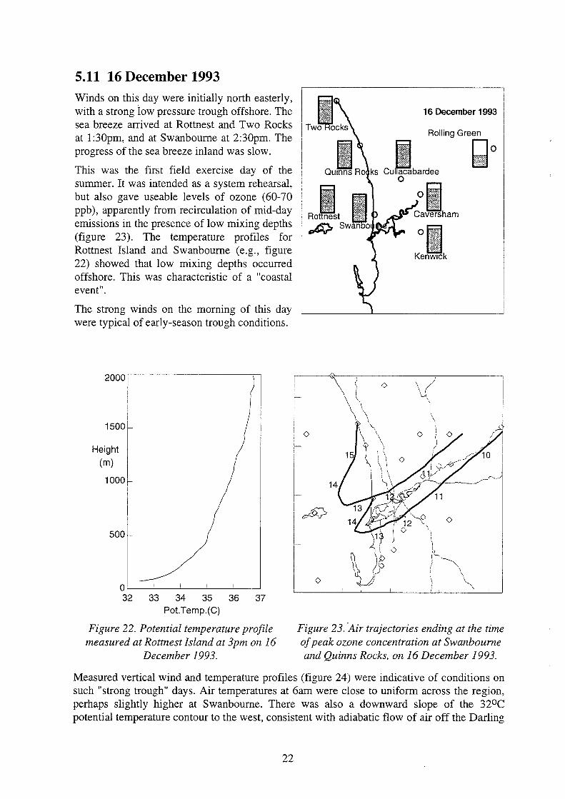
5.11 16 December 1993 Winds on this day were initially north easterly, with a strong low pressure trough offshore. The sea breeze arrived at Rottnest and Two Rocks at 1 :30pm, and at Swanboume at 2:30pm. The progress of the sea breeze inland was slow.

This was the first field exercise day of the summer. It was intended as a system rehearsal, but also gave useable levels of ozone (60-70 ppb ), apparently from recirculation of mid-day emissions in the presence of low mixing depths (figure 23). The temperature profiles for Rottnest Island and Swanboume (e.g., figure 22) showed that low mixing depths occurred offshore. This was characteristic of a "coastal event".

The strong winds on the morning of this day were typical of early-season trough conditions.

2000

1500

Height

(m)

1000

500

0 '---~--'------'-------''----' 32 33 34 35 36 37

Pot.Temp.(C)

Figure 22. Potential temperature profile measured at Rottnest Island at 3pm on 16

December 1993.

16 December 1993

Iii Romng Greri O

Ouinns Ro ks cJ!!bardee 0

oi;J ,,tM<

Caversham

0

0

Figure 23. ·Air trajectories ending at the time of peak ozone concentration at Swanbourne and Quinns Rocks, on 16 December 1993.

Measured vertical wind and temperature profiles (figure 24) were indicative of conditions on such "strong trough" days. Air temperatures at 6am were close to uniform across the region, perhaps slightly higher at Swanbourne. There was also a downward slope of the 32°C potential temperature contour to the west, consistent with adiabatic flow of air off the Darling

22

Scarp. By noon the easterly and potential temperature were well mixed, and at 6pm a shallow sea breeze inflow was evident.

Westerly wind component (m s-1) Potential Temperature (°C) 0600 890---~--------------~ 890,------------,-,,...,---------,

: : .

915 "'I,,~,,_;

940 940 ·. ·.

965r---i~

990,-...--22~

4 0

350 360 370 380 410 420 430 350 410 420 430 440

1200 890-~--------, --; ------~

h ,~ r ~

965~( ._;..-----:~~:=-: 990 '

' -6 -----

915 915

940

965

990

\ 34

I 350 360 370 380 420 430 440 350 420 430

1800 890,-----,-----------,--,------------,

f----o--...._

915

940

350 360 370 380 420 430 440

Figure 24. Onshore and vertical wind and temperature profiles for 16 December 1993, as measured by radiosonde, sodar and RASS systems. The height

coordinate is pressure in hPa. The vertical shaded lines are measurement locations. No potential temperature profile is given for 1800 WST due to lack of

spatial detail.

23

440

5.12. 22 January 1994

This was a Sunday, with low levels of urban emissions, particularly during the crucial 6-9am period. Elevated ozone values at many sites about the metropolitan area appear to have been due to bushfire smoke.

Below, along with the Caversham ozone plot are shown nephelometer measurements of haze from the Caversham and Hope Valley sites, for 22 January. Relatively high haze levels in the morning were probably due to a bushfire to the south of the city. Trajectories to Caversham passed through this region during the night and

. . previous mommg.

22 January 1994

Cullacabardee Rolling Green

Ouinns Rocks

[i Swanb urne .

.

Rottnest Caversham

~ I ' Kenwick

120,--------------------------1 oo Ca.v..e1sbamA.,O.M.S.~------/,.1---------ao

Ozone 60 (ppb) 40

20 o -~-----""'o~=.;_;__;_..;;.;,.;_=

5 4 .. Caversham A.Q.M,S.

Visibility 3--------------------------(Bsp) 2 ..

1 ·······························

2 4 .............. - .................... ·-······-------······· ........................ - .. __________ _

Visibility 3 .... Hope.Valley A.Q.M.S.

(8spl 2+------------1031-----------------

Figure 25. Ozone and visibility measurements at DEP sites on 22 January 1994.

24

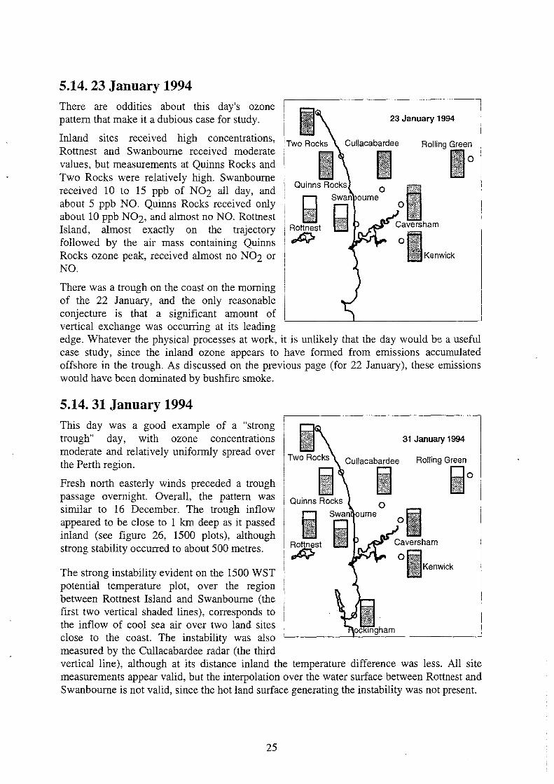
5.14. 23 January 1994

There are oddities about this day's ozone pattern that make it a dubious case for study.

Inland sites received high concentrations, Rottnest and Swanbourne received moderate values, but measurements at Quinns Rocks and Two Rocks were relatively high. Swanboume received IO to 15 ppb of NO2 all day, and about 5 ppb NO. Quinns Rocks received only about 10 ppb NO2, and almost no NO. Rottnest Island, almost exactly on the trajectory followed by the air mass containing Quinns Rocks ozone peak, received almost no NO2 or NO.

There was a trough on the coast on the morning of the 22 January, and the only reasonable conjecture is that a significant amount of vertical exchange was occurring at its leading

I 23 January 1994

Two Rocks Cullacabardee

I . I . .

Rolling Glree~

. .

.

• Ill Rottnest

~

0 Swan ourne

n lit

0

Caversham

01:··.•· : ~

:J«ti Kenwick

edge. Whatever the physical processes at work, it is unlikely that the day would be a useful case study, since the inland ozone appears to have formed from emissions accumulated offshore in the trough. As discussed on the previous page (for 22 January), these emissions would have been dominated by bushfire smoke.

5.14. 31 January 1994

This day was a good example of a "strong trough" day, with ozone concentrations moderate and relatively uniformly spread over the Perth region.

Fresh north easterly winds preceded a trough passage overnight. Overall, the pattern was similar to 16 December. The trough inflow appeared to be close to 1 km deep as it passed inland (see figure 26, 1500 plots), although strong stability occurred to about 500 metres.

The strong instability evident on the 1500 WST potential temperature plot, over the region between Rottnest Island and Swanboume (the first two vertical shaded lines), corresponds to the inflow of cool sea air over two land sites close to the coast. The instability was also measured by the Cullacabardee radar (the third

Cullacabardee

31 January 1994

Rolling Green

0 i s~:n ourne

Rottnest ii ~ oil .. • · '. Kenwick

4f .. f-

0

vertical line), although at its distance inland the temperature difference was less. All site measurements appear valid, but the interpolation over the water surface between Rottnest and Swanboume is not valid, since the hot land surface generating the instability was not present.

25

Westerly wind component (m s-1) 0600 890 r====::::=---.._,-----,-=~-------,:,,.---,--,

965

350 360 370 380 410 420 430 440

1200 890.==o==-------,---:~--.;:--w.....,..._....,,-~---,--,

'" ·~-{f~f 940

ri 965Lr-T rr . ____ ) 990 r=-r::::,,. _4 --~--

350 360 370 380 420 430 440

1500 890r---,-------,r----,-,--,----,-----,--,

915 ~< i l

> 990 ' ~~' /,

350

Potential Temperature (OC)

890-------------------; :

915

940

965

' . ' i~

L:r[l~ i'----30~

30 ~ j--2B__j~28 :

990 1=--;..-26---'----;--

l----o--24----'----;--

350 360 370 360 390 400 410 420 430 440

890 ...-~-------,----,----------, C • •

915 : \ :

940

~ ?8 j

36 ·.·\• I\ I '. . "' ; ; ' ; 3~ i

965

990

350 360 370 380 430 440

890 -------------,------,------,

915

940

38

~L

430 440

Figure 26. Onshore and vertical wind and temperature profiles for 31 January 1994, as measured by radiosonde, sodar and RASS systems. The height

coordinate is pressure in hPa. The vertical shaded lines are measurement locations.

26

5.15. 4 February 1994 Ozone concentrations on this day were moderate, but the event was significant because it was the only smog event within the intensive study period of the 1993-1994 summer.

Easterly to north easterly winds preceded the sea breeze, which arrived at the coast 10am. A westerly to south westerly sea breeze direction ensured that urban and Kwinana emissions remained separate (figure 27). Unusually, winds were lighter offshore than at the coast (figure 28).

The day appeared a fairly useable example for study, although ozone levels were low due to cool temperatures. Levels of nitrogen oxides were significant in urban plume. The smog cloud was tracked by aircraft to Goomalling.

The event was close to an "inland event" pattern, but for the low temperatures.

~ Two Rocks

n Ill

4 February 1994


i , . [i o " . .

Quinns Ro ks 0 n • Rottnest

~

./ \\

l \

\ !

\.., \

Kenwick

Figure 27. Calculated air trajectories ending at Caversham at 12:30pm, and starting from the Hope Valley site in Kwinana at 8am, on 4 February 1994.

27

Figure 28. Windfields at 8am (pre-sea breeze), 10am (sea breeze formation) and 2pm (well developed state) on 4 February 1994.

In figure 29, the offshore velocity contours show horizontal convergence was present both at 6am and 12 noon. Information available for 3pm indicates a more uniform flow field.

As for the 19 February case (see page 30), stability at 6am was lower offshore than over land. This is presumed to be an effect of the coastal trough. There is a uniform trend of an increase in the height of the layer of greatest stability, from the airport to Rottnest. At 12 noon atmospheric stability was less offshore, but at 3pm it had again increased, with the approach of a cool air mass at the surface, and a slight warming of the layer from 500 m to 1000 m.

28

Westerly wind component (m s-1) Potential Temperature (OC)

0600 890 r-------c,.,,...----c-, --. --~---c-.

~8 ! l 915~2~! •

940 ~~ ~~~~? o~~-1

965

990 0 l---'---18~ i

'' 360 370 380 410

1200 890 .----,----:,,....--c---:;a.----,-~---,.------,--,

\.~

350 360 370 380 430 440 350 360 400 410 420 430

1500 890 ----------------.-----,

l---'--6---:--1

915

890

i ---/26

915

J_) 940 8 24--

940!-22_

965 ,__ __ C86 l

990

350 360 370 380 410 420 430


coordinate is pressure in hPa. The vertical shaded lines are measurement locations - from left to right, Rottnest Island, Swanbourne, Cullacabardee, Perth

Airport, Gidgegannup and Rolling Green.

29

440

440

440

5.16. 19 February 1994

The day began with north to north easterly winds, and a weak trough offshore. The sea breeze was initially north westerly, arriving about 10:30am. The trough passed inland about 1 :30pm (figure 32).

This was the biggest "smog event" of the season. An accumulation of nitrogen oxides formed the previous evening in light winds, and was carried well offshore by morning. The advance of the trough was delayed due to the effects of an approaching cold front (Pressures fell west of the trough - note the weak gradients in this region in figure 33).

The urban plume passed over the Rockingham site, giving an hourly peak just over 80 ppb. Then from 3pm the trough passage brought high levels to the whole coastline, from

Rottnest A:,

19 February 1994


i .• ~ Ill

Cavers ham

• llJ Kenwick

i

Rockingham to Two Rocks (figure 31). Quinns Rocks data are missing due to an equipment failure. Ozone was also detectable by the nose at the city at 4pm, perhaps due to reduced mixing on the along-river trajectory it would have followed. Concentrations had decreased by the time the inland sites were reached. This was a classic "coastal event".

The day was a Saturday, so the first ozone peak was probably reduced in comparison to what would have been observed on a weekday. An emissions analysis for a Friday night (Department of Transport, personal communication) indicated that vehicle emissions in the late evening on the preceding day were increased in comparison to a normal weekday. However, early evening emissions were slightly reduced, so the nett result was probably insignificant.

Temperature profiles at 6am (figure 34) showed lower stability at Rottnest, probably indicative of a trough not far offshore. The general slope of the isotachs at this time, with wind velocities decreasing both vertically and offshore over most of the plotted region, may be typical of some days with a trough present offshore. Modelling experiments using 16 December meteorology commonly showed the same wind structure within the stable layer near the surface. The strength of the onshore flow at 3pm (when the smog mass reached the coast) is also notable. The trend of arrival times of the ozone peak at PPSS stations suggested movement of the smog mass at about 10 m s-1.

30

120---------------------------1 00 Two Rocks A.Q.M.S.

80 Ozone 60 (ppb)

120 100 . Swanbourne A.O.M.S.

80 Ozone 60

(ppb) 40 +------------20 ..._--------~--<, 0 -+::-------::0:t::6=~~~

120------------------·---------100 N. Rockingham Intensive Stud~, _______ ,._ _________ _

80----Ozone 60 1--------------,,

(ppb) 40 +-----------1 20 t------i~l---------,~b

O -k---1..:.;.:;.Q,-=:::::,,.-::0:+.::6-.:::Z...:.=---,t;;;;,;;.

Figure 31. Ozone measurements at three of the coastal monitoring sites on 19 February 1994. The upper two show effects of the trough passage only; the lowest

shows effects of both the sea breeze and trough passage on ozone levels.

DATE.: 190294 TIME: 08:00 DATE: 190294 TIME: 15:00

Figure 32. Windfields before the sea breeze, after sea breeze fonnation, and after trough passage, on 19 February 1994.

31

25,-------,------,-----:-..---------,-------,---,------,-,::-,r--,-----:---,-:=.--,--,--,---,---,--,---,----, . H: .

.. ........ , ...... )( .. ;------·

. [1011]

L

115 125

Figure 33. Suiface pressures, hPa, at 6am on 19 February 1994.

32

Westerly wind component (m s-1) Potential Temperature (0 C) 090,---~-----,------------,

915

940 940

965 965

990 990

350 370 380 430 440 350 420 430 440

01200 890 ,-------~-----------,--, 890,---------,------------,

915

940

965 965

990b I 2 4

1----6-----'-.-

350 360 370 380 430 440 350 360 370 380 430 440

01500 890,==~-----=----------,------, 890,---,------:::,--------------,

915

940

915

940

965

~ 34

32 : • ~ 30~. >

350 360 370 380 420 430 440 350 430 440


coordinate is pressure in hPa. The vertical shaded lines are measurement locations - from left to right, Rottnest Island, Swanbourne, Cullacabardee, Perth

Airport, Gidgegannup and Rolling Green.

33

5.17. 3 March 1994

Morning east to north easterly winds preceded a sea breeze at coastal sites at about noon. The day was expected to produce a major smog event, but the morning winds were stronger than predicted, and a radiosonde release exercise was cancelled.

Late in the day, hourly averages close to 80 ppb were detected at Quinns Rocks and Two Rocks. The general character of the day was comparable to that of 19 February, and it Ro.!lJJ.est

clearly represented a "coastal event". ~

Trajectories to coastal sites suggested that smog originated in the northern suburbs, but they passed to west of Rottnest, and it is probable that winds were more southerly in the trough, to the west. It is likely that northern ozone arose from urban emissions, while slightly lower concentrations in the southern part of the region affected came from K winana.

3 March 1994


mffl 0

ol) Cavers ham

oQ Ill

Kenwick

no 11!1

Figure 35. Calculated air trajectories ending at times of peak ozone concentrations, at Swanboume, Quinns Rocks and Two Rocks, on 3 March 1994.

34

5.18. 4 March 1994

Morning winds were easterly to south easterly, and light offshore. The coastal trough reached Rottnest at 10:30am, and Swanboume at 1pm

A smog event was not expected, due to the initial south easterly winds. However, a 72 ppb hourly average at Two Rocks occurred between 1 pm and 2pm, and must have been due to K winana emissions, and the light winds offshore (figure 36).

The day was therefore grouped in the "K winana event" class.

\ a

8 V

Two Rocks

i \ !

i . . .

,·_,,.,.,..,,,.-./

,/ I ,,

,__... .,-'

4 March 1994

Caversham on Iii

Kenwick

Figure 36. Calculated air trajectories ending at Two Rocks on 4 March 1994 ending at 12 noon, 12:30, 1:00 and 1:30pm

35

5.19. 8 March 1994 Winds commenced light southerly, then turned westerly to south westerly. The coastal trough was predicted to pass inland during the day, but the movement occurred about 3am. A field monitoring exercise was called off after an initial radiosonde release, at 6am from Swanbourne.

However, winds remained light, and Rolling Green received a 74 ppb hourly average from the overnight/morning accumulation.

This was one of the few "light westerly wind" events.

~ Two Rocks

n Ill

Quinns Rocks n Swanb

Ill n Rottnest bid ~

i

V k i '-·-~"'-,, ; \ I , \ \ ; \....\ i I

8 March 1994


~ 0 on

II

l o .

Caversham on lid

Kenwick

Figure 37. Calculated air trajectory ending at Rolling Green at the time of peak ozone concentration on 8 March 1994.

36

5.20. 12 March 1994 The day commenced with the coastal trough located close to the coastline, with winds initially northerly inland.

A smog event was expected, but no special radiosonde measurements were possible because hired equipment had been returned. However, an additional radiosonde release from Perth airport was requested. The RASS temperature profiler at Cullacabardee was also out of operation. There was a IO-minute ozone peak of 132 ppb at Swanbourne and 89 ppb at Kenwick (figure 38). However, events were very short, with hourly averages were both about 80 ppb. Trajectories from urban locations passed to the south of the network (figure 39). This suggested that higher values may have occurred undetected, in the southern coastal suburbs.

12 March 1994

Cullacabardee Rolling•: [:;J

111 0

oiJ.•.li"''' ;1:1~ .·t:.,.(

Caversham

Kenwick

Ill

The day is probably best placed in an interim class between "inland". and "light westerly". It is the sole case recorded of peak smog levels in the southern suburbs.

120-------------------------100 +-K=e'-'--nwcc.ci=ck.c.c.A~.Q=·=M=.Sc..c.. __________________ _

80 +---------------------------Ozone 60 (ppb) 40

20 0 -i<------~-...:;...----=---"-"

120------------~-------------100 __ SwanboumeAQ.M.S ...

80 Ozone 60

(ppb) 40

20 ·--·-·-·····-----·-·-----0 -~.__----~-=::::.:.="'"'

Figure 38. Ozane concentrations measured at Swanbourne and Kenwick on 12 March 1994.

37

Figure 39. Calculated air trajectories ending at the times of peak ozone concentration at Swanboume and Kenwick, on 12 March 1994.

38

5.21. 16 March 1994 This was the first of a sequence of smog days, resulting from the presence of a tropical cyclone (named "Sharon") in the Indian Ocean, off the north west coast. The larger-scale pressure effects of the cyclone allowed the coastal low pressure trough to remain just offshore.

Morning winds were easterly, temporarily quite fresh due to a small-scale feature in the trough. They eased after 9am. By 1 0am there was a clear south easterly tendency m winds measured at Rottnest.

Possibly due to the non-uniform effects of the initial easterly, there was a considerable variation of sea breeze arrival time at the coast. It was first detected at Two Rocks at 11am, Rottnest at 11 :30am and at Swanbourne at 1 pm

The sea breeze brought in a large "pool" of

I . . . Two Rocks

I . Quinns Rocks

[;J Ill

Rottnest

~

16 March 1994

Cullacabardee

I . . Rolling Green

lo .

.

.

0

I 0 .

Kenwick

smog at the coast, of moderate (about 60 ppb) levels, which reacted with urban daytime emissions to give the first high Caversham smog levels of the 93-94 summer season. Air trajectories indicated a contribution by mid-morning emissions from the Kwinana industrial area (figure 40).

\ ; \j

\

\1 \

I I ,r' i !

) ;_;

/ _/__,_,

i r-// ~/ ;

,· . .,...l._'--... ·---·---·-,/..,_;·~-"

Figure 40. Calculated air trajectories ending at the time of peak ozone concentration at Cullacabardee and Caversham, on 16 March 1994.

39

5.22. 17 March 1994

The day began in a typical pattern for a smog event, with an initial southerly at Rottnest, which reached the coast at 9am. Winds were initially light and variable inland.

There were high NOx and haze levels around the metro area. The latter was consistent with a report from Bushfires Board of a fire south of Armadale the previous day. The apparent haze plume was narrower than normal, supporting a nearby smoke source.

Calculated trajectories ending at Rolling Green and Caversham, at the time of their ozone peaks, only pointed offshore and south, into the trough (figure 41). A trajectory from Kwinana passed Caversham at 11:30am (also shown in

17 March 1994


0

n Swanb urne

mi n Rottnest Ill

0

~

Kenwick

figure 41), the time of peak NOx concentration (30 to 35 ppb). This indicated that Kwinana emissions passed inland ahead of the smog mass, and did not contribute greatly to smog formation on the coastal plain.

It was possible to generate a trajectory from Kwinana to Caversham, ending at about 12: 10pm, by using 10-metre winds rather than those for a higher level. The use of 10-metre winds to represent boundary layer transport is, however, unrealistic. In addition, using 10-metre winds, the source region of the NOx peak at 11 :30am is implied to be the Kwinana freeway and eastern metropolitan area only. This appears too small for credibility.

The day would have been classed as a "light westerly" day, on the basis of the apparent non-interaction of Kwinana emissions with other smog sources. However, the presence of smoke required grouping in the "bushfire" class.

40

\ \ i ) f

Figure 41. Calculated air trajectories ending at the time of peak ozone concentration Rolling Green (2:30pm), and the time of peak NOx concentration at Caversham

(11:30am).

5.23. 18 March 1994 This day also commenced with an initial southerly at Rottnest, and winds light south easterly to easterly inland. The sea breeze arrived at the coast at 11am, but stalled at the Darling Scarp about 4pm.

50-60 ppb of NOx passed offshore through Swanbourne in the morning, but dispersed before passing inland on the northern beaches. An inflow of about 50 ppb of ozone plus 20-30 ppb on NOx arrived at Swanbourne with the sea breeze. These levels were maintained at this site through the afternoon.

When the air arrived at Cullacabardee, it had reacted to give a 110 ppb ozone hourly average. Caversham received 89 ppb, and Kenwick 76.

• Swa~,b urne

Ill • Rottnest Ill ~

18 March 1994

RollingGrn

O

0 I . . Cavers ham

Kenwick

Ill

A brown NO2 plume was observed by the author in the afternoon, passing from K winana along the coast at the top of the sea breeze. There were no indications of abnormal operation of any Kwinana industry. A large plume of NO2 was also seen from Perth, moving inland from Kwinana. It was perceptibly shallow, but its visible length occupied a major fraction of the distance from the coast to the hills. Swanbourne NOx and ozone rose slightly from 2:30pm. This was perhaps an effect of the observed NOx plume.

Because of the role of plumes from Kwinana, this day was classed as a "Kwinana" event.

50~-----------------------····-····-·················•···

40

NO230

(ppb)20~•················-····-·--·•········-········----rc

50..----------"-----------------

40 ·········

NO 30+---------1----------------(ppb)20t-----------,f/!c;.l n-----------------

10 ····················

0-~~-=------~~-"' 2

80

60+-------------------------Ozone40

(ppb) 20

Figure 42. Concentrations of nitrogen oxides and ozone at Swanbourne on 18 March 1994. Significant features are the relatively steady concentration of nitrogen dioxide (N02) in the

morning inflow, and the rise of all values in the late afternoon.

41

With the lack of measurement sites, the temperature and wind velocity contour data for this day were rather sparse. The wind velocity plot in figure 43 is based only on data from Cullacabardee, Perth airport and Gidgegannup. Temperatures are from Perth airport alone. However, there is a clear indication of a velocity peak of about 12 m s-1, at about 400 metres' height, uniform over the coastal plain and at the level of the inversion at the airport. Modelling work has suggested that the strongly stable layer at about 500 metres' height (near the 965 hPa level) was important in maintaining a shallow sea breeze inflow, later in the day.

Also shown, in figure 44, are the wind and temperature records from the airport, at 7am and 1 pm. A shallow sea breeze inflow and inversion are evident on the latter.

Westerly wind component (m s-1) Potential Temperature (°C) 0600 890,---,----------------,.-.-,

915~! '.! ! :. '.

890r--,,..--------,------,-----,--,

-~-34--~-~-

i -4--'--L ' -6 ' ' '

915

940~ : -8 ! ! : 940

>=====;*;;:;;;;;;;;;;;;;;~~~~~~~ 9651----•12 -----,--~

-~--10-------... 965F'.··. ii============

990

350

4 0

430

' 24---;---'

990 . I •

350 420 430 440

Figure 43. Onshore wind velocity and potential temperature profiles on 18 March 1994. Only a single temperature profile site operated on this day.

2000

1500

Height (m) 1000

500

20001

1500~

1000

500

20 25 30 35 40 0 4 8 12 0 100 200 300

2000------, 2000 2000

1500

Height (m) 1000

500

1500

1000

500

1500

500

I

I

I

~ O 34 35 36 37 38 39 0 0 4 8 12 16 O 0 100 200 300

Temp.+ DALR*height (amsl) Speed (mis) Dir'n (deg)

Figure 44. Temperature, wind speed and wind directions measured at Perth Airport on 18 March 1995, at 7am (top) and 1pm (bottom).

42

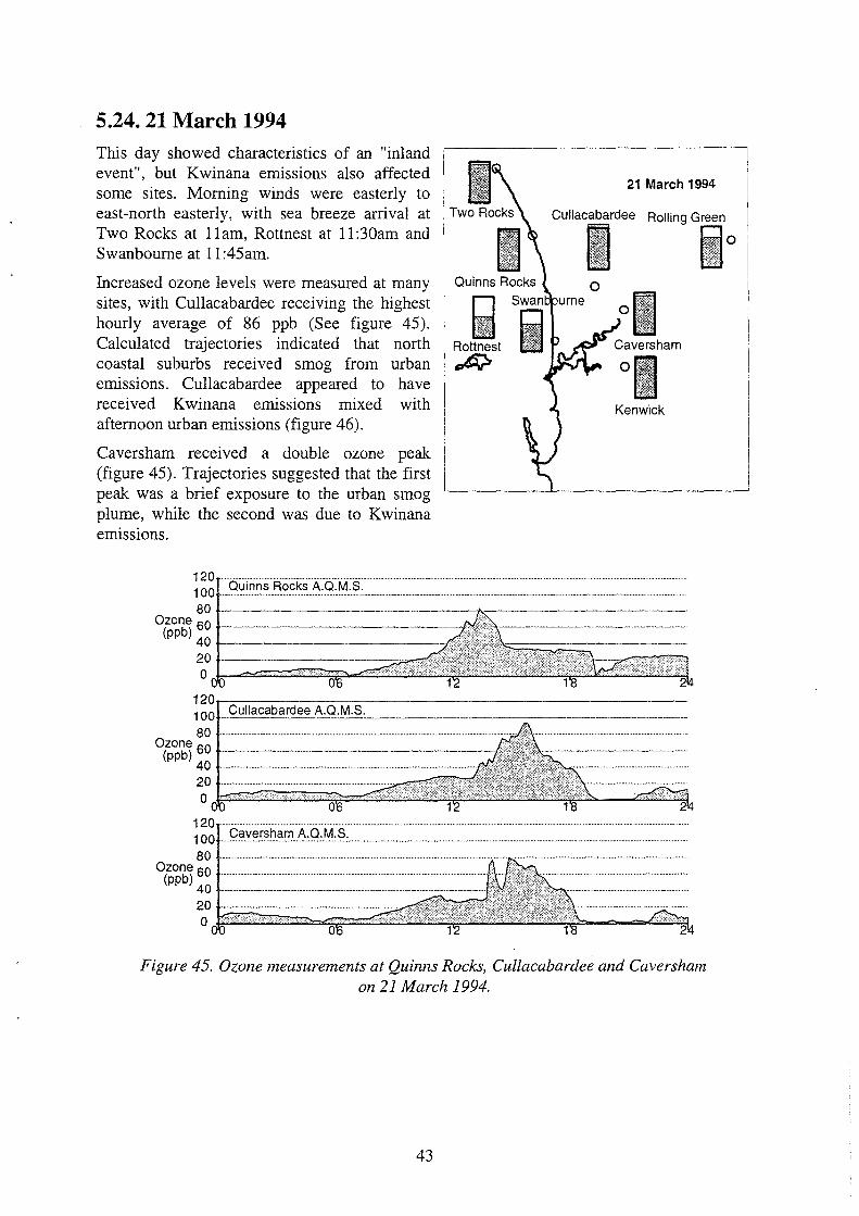
5.24. 21 March 1994

This day showed characteristics of an "inland event", but Kwinana emissions also affected some sites. Morning winds were easterly to east-north easterly, with sea breeze arrival at Two Rocks at 11am, Rottnest at 11:30am and Swanbourne at 11 :45am.

21 March 1994

Cullacabardee RollingG~

O

Increased ozone levels were measured at many sites, with Cullacabardee receiving the highest hourly average of 86 ppb (See figure 45). Calculated trajectories indicated that north coastal suburbs received smog from urban emissions. Cullacabardee appeared to have received K winana eill.lss10ns mixed with afternoon urban emissions (figure 46).

Caversham received a double ozone peak (figure 45). Trajectories suggested that the first peak was a brief exposure to the urban smog plume, while the second was due to Kwinana emissions.

• II) Rottnest

~

0

I 0 .

Cavers ham

Kenwick

120 ··············•··················--·······································•·· 100 ... 9!:J .. i~.~s Rocks A.Q:~.:.§l_. _______________ _

80---------------------------0zone 60 +-------------------1

(ppb) 40 +---------------,'', 20t-----------==~~, 0 nk--===:z:::~-=:::::::I!.:.~~~~~~~~~~~~~. 120..---------------------------

Cullacabardee A.Q.M.S. 100--------------------------80

Ozone 60

______________ _

(ppb) 40 .............................................................................................................................. ..

20n1~--.. =·= ... i ... :::: .... :: ... i. .. i.----=--=····~ .... ;:;;;; ... .;,, ..... .;,, ..... :::i. ... == .. --•'1::.·~-~~ 0

120 ... 100 .. q~Y'?r.~~-~r.i:t ... A:O.M.S.

80 Ozone 60

(ppb) 40 +--------------

fJlj

Figure 45. Ozone measurements at Quinns Rocks, Cullacabardee and Caversham on 21 March 1994.

43

(a)

0

\/ ''--\

\

\ \

Figure 46. (a) Calculated trajectories ending at the time of the smog peak at Quinns Rocks and Cullacabardee and (b) at Caversham about the arrival times of

the two peaks detected there.

5.25. 14 April 1994

This event occurred well after the normal end of the period of the year when smog events occur. It appears to have been due to a combination of light winds and unusually warm temperatures, which allowed mixing depths to remain low offshore.

The day started with light easterly to east-north easterly winds. A sea breeze developed at Two Rocks at 11am, and at Swanbourne at 12 noon. Directions changed through north at the coast, and winds inland remained northerly.

Relatively high concentrations of NOx (10-minute peak of 75 ppb) passed offshore at Swanbourne, as a result of the morning traffic peak. The IO-minute peak of ozone in the return flow at Swanbourne was 88 ppb. Increased ozone levels also were measured at Quinns Rocks.

44

i . . I . C

Quinns Rocks

Rottnest

~

14 April 1994


0 • Ill

0~ II Caversham

0

Kenwick

5.26. 16 December 1994 16 December 1994 Ozone peaks. at Cullacabardee and Caversham

occurred in coincidence with the arrival of the sea breeze, but background levels beforehand were about 10 ppb higher than normal. This suggested that some photochemical reactivity was present in the background air, due possibly to bushfire smoke or a high level of biogenic emissions. There was only a small amount of smoke haze present, however (figure 47).

[i Cullacabardee

I . . . . Rolling iGreen

. .

Quinns Rocks

~ Swanb urne

Rottnest Ii Caversham

Trajectories to Cullacabardee and Caversham led back to K winana, so the day was classified as a "Kwinana" event.

~ i . . Kenwick

Cullacabardee A.O.M.S. 120T--'-'---'--'_:._-'-'-..:._..;_.=;~;;_c_------------- ---100+---------------------------80+-----------------

0zone 60 ---------------(ppb) 40 -----------=

20 0

120 Caversham A.0.M.S.

100+---------------------------80+---------------------------

0zone 60

(ppb) 40 1--------------~ 201;~~~~t0,t,7.'"';~ .... ~~f:cJK0:~I 0 tffi"''--------'-'-......... =---'1,:if""'-"""'=-="-'--~=-=:..=

5 _ __,__-'-'---...,__Ae-.Q--'-._M=.S=---·-------------------

4

Visibility 3r-------------------------(Bsp) 2+-------------------------

4

1

o~c:::::z=E==::==;;;:;:::::::===~=====:==~;;z:=~:mE~~4

Figure 47. Ozane concentrations at Cullacabardee and Caversham, and visibility measurements at Hope Valley, on 16 December 1994.

45

5.27. 17 December 1994 17 December 1994 Ozone levels on this day were enhanced by the

effects of bushfire smoke. Visibility measurements with peaks in the Bsp range from 1 to 1.5 were measured at Kenwick, Swanbourne, Duncraig, Hope Valley, Caversham and Queens Buildings, both overnight from about 2am to 6am, and in the afternoon at about 1pm (e.g., figure 48).


This case was classified as a bushfire smoke event.

120 ···········································•··················

. -

Quinns Rocks

Swan ourne .• Rottnest Bl ~

Cavers ham 01 Kenwick

100 _c_ul_la_c_ab_a_rd_e~e_A_.Q-'-'-.M_.S __ . _______________ .... __ .. _. __ ···-•-····

80 Ozone 60

(ppb) 40 --

20 o~::L:::::::.:::=~G±JGJ.G..~~~i:J.it:GE~::=::::::::::::::::...~

4 120· __ .................................................. __

100 ..... caversham .. A.O.M ... s.

80 +-------Ozone 60 __________ .,

(ppb) 40 ----20 +-----------=~"'<'< o~::::::=:::.:::::::::::::::::::~~~~~~~~LL:.::.LL.~~:::::::..-c::::=..~4 5 ~------•••••••••"••••••• .. •--••n••••-••.,••••••••••••--------

4 _ Ho__ee ValleJ1'--A_._o_.M_._s_. _________________ _

Visibility 3

(Bsp) 2 ------•••••••-_,,,,,_,_,_,,.,,,,,,,,.,

Figure 48. Ozone measurements at Caversham and Cullacabardee, and visibility measurements at Hope Valley, on 17 December 1994. The steady rise of concentrations through the morning is typical of bushfire smoke events.

46

0

5.28.16 January 1995

16 January 1995 Trajectories to Caversham, Cullacabardee and Rolling Green at the time of peak ozone concentrations all came from the south, passing over K winana and parts of the metropolitan area. There were no significant haze levels at any point in the haze network, but it has been noted by Johnson (personal communication) that the reactivity of bushfire emissions can persist long after particulates have disappeared.

Cullacabardee

I . . . Rolling Glreen

. -.

.

Caversham The trend of ozone time sequences (figure 49) is notable. At Cullacabardee, there was a steady trend of rising concentrations through the morning, to a peak at about 11 :30am. This form is typical of bushfire smoke events. Caversham, in spite of a data gap, also shows clear indications of a lesser morning rise, following the bushfire smoke pattern. At Rolling Green,

I . . . Kenwick

morning concentrations (representing only rural background) rose to 60 ppb - a clear smoke effect - but subsequently the trend was closer to the pattern expected of a normal smog event, with a concentration rise at sea breeze arrival.

Indications are that the day was a "Kwinana event", augmented by bushfire smoke.

~ ;~ .. f.3.C?_l!i.~.9. .. §..r.~.~~ .. '.\:9}~_-S_. ______________ _ 80 ----------------

Ozone 60 1--------------=-------(ppb) 40

201"7x~~~~~ 0 ,4.,.;.-=====~,..;:...===== 120-r-----------------------------1001'--'C~a~v=er=s~ha=m~A~.Q=·=M=.s=-·~-----A--------------80

Ozone 60 ............................................................................................................... .. (ppb) 40 + ................................................................................................... ::;-,'""···

201;;~~~~~~ 0 ~=====....,..,,..;:...---'-'-1.---

120 100 . Cullacab~r.c:l.~~ .. r.\.9:.r-A.S. 80

Ozone 60 (ppb) 40 ?----------,..

2o0 £Ji;i;;;;;2:s:1Jzf~f!J!!J..!f.'tf"2

Figure 49. Ozone concentrations at Rolling Green, Caversham and Cullacabardee on 16 January 1995. The shaded line in the data gap for the

Caversham sequence indicates the probable data trend.

47

4

4

4

5.29. 17 January 1995 The trajectory to Rolling Green at 6pm, the time of the ozone peak (figure 50), passed from the Kwinana industrial region, and wholly south of the metropolitan area. Background reactivity was a little higher than usual - indicators of some enhanced biogenic or bushfire influence.

Kenwick showed an interesting double peak, the central maximum clearly removed by . a strong plume of nitrogen oxides (figure 50). The calculated back trajectories to Kenwick at 3:30pm to 4pm scanned across the Kwinana region, at 4pm passed north of the industrial area, and at 5pm passed over the BP refinery. The logical conjecture is that the first peak was due to general Kwinana emissions, the dip was due to the combined effects of the trajectory passing north of the region, with power station

17 January 1995

Cullacabardee

I Rolling Green

I Quinns Rocks

Swan ourne

ii . R~t

[I . . Caversham

li . . Kenwick

NOx emissions added, and the later peak was due to lower NOx and higher reactivity from the southern part of the Kwinana region.

The day was classed as a Kwinana event, with a small bushfire contribution possible.

50 ------------------40 Kenwick A.Q.M.S.

--·-······-······----·- ·······-··----·---··-·· -----

NO2/NO 30-t-------------------c (ppb) 20-t-----------------

10~-------

0 120 ............ ,., ................... , ..

100 Kenwick A.Q.M.S. __ .

80+---------------------------Ozone 60

(ppb) 40 +----------------,=~ 20

100 Rollin Green A.Q.M.S.

Figure 50. Ozone measured at Rolling Green, and ozane and nitrogen oxides at Kenwick, on 17 January 1995.

48

5.30. 18 January 1995 Ozone levels at Caversham rose earlier than normal on this day. The time of the rise corresponded to arrival of the CBD peak morning emissions parcel, but it was smaller, and the peak was broader, than usual. A later trajectory (passing Caversham at 11 :30am) passed over K win an a.

Bushfire smoke was detected in the visibility trace at Kenwick at 3pm, but was of local origin, and occurred after the ozone peak.

Ozone concentrations before the main peak indicated that background reactivity was a little higher than normal, but urban and K winana emissions were apparently the crucial factors.

The case was classified as a "K winana event", since these normally involve both urban and Kwinana emissions.

120 ······································· ..... . 100 __ Rolling Green A.O.M.S.

• [11 Rottnest

A:t

80 -------------~ Ozone 60 +----------------

(ppb) 40 ,----------= 20 0

18 January 1995

Cullacabardee

I . Rolling Glreen

.

& .

Caversham

I . .

.

Kenwick

2

100 Kenwick A.Q.M.S. ------------------------

80 Ozone 60 -------------,

(ppb) 40

2o0

JJiJJ.:'.j_'°tJ?:J.T:.J:.~.;;.7:2.J.~~:::,~ :;..;;. :;""-~fl: .. f=J}.

120 100 80

Ozone 60 (ppb) 40

20 0

Caversham A.O.M.S.

.... , ..................... __ _

Figure 51. Ozone measurements at the three stations where the highest values were measured on 18 January 1995.

49

5.31. 31 January 1995

31 January 1995


Ii Ouinns Rocks

The calculated air trajectory ending at Rolling Green at 12 noon passed through the southern suburbs, then north eastward along the Swan river before heading to Rolling Green. The trajectory ending at 1 :20pm passed through Kwinana, while the rest of the afternoon's trajectories passed through the Perth region along the length of the Swan River. High ozone levels at Rolling Green were logically due to a combination of Kwinana and urban emissions, reaching their destination at the time of maximum smog production.

~ Sw:n ourne

Rottnest l~~J Caversham

The steady upward ozone concentration trend, although often a characteristic of bushfire smoke events, is probably in this case indicative of the increasing source strength, for the sequence of trajectories involved.

~ • II Kenwick

120--------------------------100 -80 ~ .............................................................................................................................. -.,;,

Ozone 60 ---------------,-.,: (ppb) 40

20

2

Figure 52. Ozone concentrations at Rolling Green on 31 January 1995.

5.32. 10 February 1995

This was a clear "coastal event". Calculated trajectories indicated that Rottnest and Quinns Rocks ozone concentrations were due to both urban and Kwinana emissions. Peaks at both sites were broad, consistent with an initial urban source, followed by a later Kwinana contribution.

50

1 O February 1995

Rottnest

~

Kenwick

5.33. 12 February 1995 This was an event clearly affected by the reactivity of bushfire smoke. Figure 53 shows haze time sequences at southern measurement sites on this day, with large peaks mid-morning and about noon, and figure 54 shows the highest ozone peaks in the meteopolitan area, which resulted. The Rolling Green site would probably also have experienced high ozone levels, but suffered an equipment failure on this day.

Visibility

(Bsp)

5 Kenwick A.0.M.S.

5 ···•···················

4 Hope Valley A.Q.M.S.

Visibility 3

(8sp) 2 ··········

12 February 1995

Cullacabardee

i . . Caversham

I . . . Kenwick

----·· .......................... .

2

Figure 53. Nephelometer visibility measurements at Hope Valley and Kenwick, on 12 February 1995.

120T-------- -------~··-·····-·····-····--······--··-······--· ---100 Kenwick A.0.M.S.

80 t---·-----------j Ozone 60 +-------------

(ppb) 40 +------------=

20 +-------------,..<'. 0 -~.:="-------,,1:,--== 120-.----------------------------100 Caversham A.Q.M.S.

80 Ozone 60 t--------------;;;f./

(ppb) 40 +------------< 20 0 J;_:::::==....::::::::::.....~=::;;;:~~r:£.;

Figure 54. Ozane measurements at Kenwick and Caversham, on 12 February 1995.

51

5.34. 17 February 1995 This was a coastal event, with high concentrations at Swanbourne, Rottnest and Quinns Rocks, and lower values inland. Calculated trajectories (figure 55) indicated that the main source of coastal ozone was urban emissions.

l ~i ,V,

Quinns Rocks

I Swan

flt Rottnest lit .,c;):,

17 February 1995

Cullacabardee RollingG~n

l;J Ill

Kenwick

Figure 55. Calculated air trajectories ending at the times of peak ozone concentration at Quinns Rocks and Swanboume: on 17 February 1995.

52

5.35. 20 February 1995 This was classified as a "stalled sea breeze" event. The ozone peaks occurred over a long period, during which calculated air trajectories came from both urban and K winana regions. The sea breeze stalled at the coast, making little progress inland until 3pm, not reaching Cullacabardee until 5pm, and Caversham at about 6pm.

5.36. 21 February 1995 This was a clear coastal event. There was an oddity, however, in that the calculated air trajectory to Quinns Rocks stayed well out of the main urban region, in the northern suburbs. The trajectories to Rottnest and Swanbourne at the time of their ozone peaks passed close to the central business district of the city (See figure 57).

One potential clue lies in the Rottnest ozone time sequence (figure 56), which shows a double peak. Calculated trajectories over the period 12 noon to 3pm (figure 57) showed no significant change in the source region, although the later trajectories passed further offshore before returning to Rottnest

A radiosonde released from Swanbourne at 1 :51 pm, within the time period of the ozone

~st

20 February 1995

Cullacabardee RollingGrr

~ Caversham

n 111

Kenwick

21 February 1995

blJ

Cullac[iabardee Rolling G~reen

c:1, ,½.t10

i . ' Cavers ham

• II Kenwick

peaks, showed nothing abnormal in the vertical wind profile. It is nevertheless possible that there was a region of more southerly wind undetected offshore, which rendered the measured trajectories inaccurate. If this were the case, the peaks at Quinns Rocks and Swanbourne, and the earlier, lower peak at Rottnest, would have been due to urban emissions, while the later peak at Rottnest would have been due to sources in the Kwinana region.

53

120r-------------------------------100 . .Quir:ir:i.".Rocks .A.·.9.:.r.-ii-.. ?..: ................................. . 80

Ozone 60 +-----(ppb) 40

120 100t------ao-------------~c:,------------

Ozone 60 t----------(ppb) 40 +------------./":'

20t:;ts=::;:::;::::::::-::::;==:::~---::::~:<,;:St'l1< 0 -~.2;.;.;.__;;;.:.....::.2;.;.;.....::.,;;;,:::=:::::::.;.;;..;;.2;.;.;.~~~.2;.;.;.~~~4~~~.c::::::..2.:.:.:.~

Rottnest Island A.Q.M.S.

801------------------~----------0zone 60 1---------------..----1.,,,•·."',------------

(ppb) 40

20 0 _..,.. _________ ....._"'----'-:='"'-------------------......,.,i::,------...;;_-----------.,.,,;-----.....,;.--,,,l2

Figure 56. Ozone concentrations at coastal sites on 21 February 1995.

i \ ; i I

Figure 57. Calculated air trajectories ending at 12 noon at Rottnest Island and Quinns Rocks ( shaded) and at 3pm at Rottn_est Island (black).

54

5.37. 22 March 1995

The day was characterised by complicated meteorology, with the coastal trough at the shoreline and wavering during the day. Trajectory calculations (figure 58) indicated that the highest peaks, at Quinns Rocks, Cullacabardee, Kenwick and Caversham, all originated from the same source region. Given the errors inherent in trajectory analysis, due to vertical wind shear, the emissions source was unarguably the Kwinana region.

22 March 1995


I Ouinns Rocks Ii Swa:b urne

Rott~=st lj ~

Kenwick

Figure 58. Calculated air trajectories to Quinns Rocks (palest shade), Cullacabardee (pale shade) Kenwick (dark shade) and Caversham (black), ending

at the site times of peak ozane concentration, on 22 March 1995.

55

6. Sea Breeze Front Movement on Potential Smog Days In the review of data collected over the 1992-1993 summer, a significant nonuniformity of the advance of the sea breeze front inland was detected. Subsequent measurements made during the later summers confirmed these observations, with some extra detail.

The analysis involved fitting a quadratic function to the relationship between sea breeze arrival time and distance inland on a west-east direction. Deviations from this fit were then calculated and displayed.

Actual advance speeds were broadly distributed (figure 59), but analysis was restricted to slow-moving fronts, typical of days when photochemical smog events occur - taken as those with speeds at the coast between 3 and 12 km hr- 1 _

25

20

(/) Q) (/) t\1 15 u -0 .. Q) .0

10 E ::s z

5

0

3 4 5 6 7 8 9 10 11 12 13 14 15 16 17 18 19 20

Sea Breeze Front Speed (km/hr)

Figure 59. Advance rates of the sea breeze front, during the 1992 to 1995 summer months.

Results are shown graphically in figure 60, as deviations of mean arrival time from the fitted value. Positive values indicate delayed sea breeze arrival, while negative values indicate early arrival.

Usually, the sea breeze arrived later inland in the northern suburbs. The first indication of this pattern was the later arrival of the sea breeze at the coast between Swanboume and Ocean Reef, but slower progress inland was also evident.

There was a smaller delay at Jandakot, also at sites on and near the Darling Scarp. There was also an acceleration of the front from the scarp to Rolling Green. All such differences are small, and may reflect no more than experimental uncertainty. However, the acceleration of the sea breeze front late in the day is a common phenomenon, and may have contributed to

56

the difference at Rolling Green. The consistency of the near-scarp values also suggests some rational cause, although topographic effects are not easily implicated, since the Middle Swan site was on the coastal plain.

-.28 •Pinjar

+.46

0 5 10 15

Figure 60. Mean variations of sea breeze arrival time (hours) at each measurement site, from the average for its distance inland. Regions where arrival

was delayed are shown shaded.

7. Conclusions The major meteorological contribution to photochemical smog events in Perth is from sea breezes, in association with the proximity to the shoreline of the axis of the west coast trough. Under these conditions, wind directions and stability characteristics combine to create conditions favourable to the return of urban emissions in relatively high concentrations.

Calculated trajectories of air reaching measurement sites at the time of smog events indicate that emissions from both the Perth urban area and from Kwinana industry contribute to smog events. The general trend is for northern suburbs to receive urban emissions, and for southern and inland suburbs to be more affected by Kwinana emissions. There are, however, important exceptions to this rule.

Smoke from bushfires also contributes significantly to photochemical smog in Perth. Trajectory analyses have indicated that, of the 37 cases analysed, between 6 and 8 would not have occurred had such smoke not been present in the Perth region. There were also a number of cases where higher-than-normal photochemical reactivity was evident before the main smog air mass arrived. Whether this was due to traces of bushfire smoke, or due to evaporative emissions of organic compounds from vegetation ("biogenic emissions"), is unknown.

Analysis of meteorological data gathered during the study has indicated that the sea breeze progresses inland more slowly in the northern suburbs. For the same distance inland, there

57

can be a delay of 30 minutes to an hour in arrival times. However, this is the only detected deviation from coastwise uniformity of the sea breeze, and is readily handled in any windfield analysis.

8. References Rye, 1995, "Contribution by Bushfire Smoke to Photochemical Smog", CALMScience Supplement (W.A. Department of Conservation and Land Management) 4, p. 129-134.

58

Meteorological and source analysis of smog events during ...

Documents

Transcript of Meteorological and source analysis of smog events during ...